Working Paper No. 218

INCENTIVE STRUCTURES IN THE PRESENCE OF SUBSIDIES: OPTIMAL CONTRACTS IN INFRASTRUCTURE UTILITIES

by

Saugata Bhattacharya* Urjit R. Patel**

Infrastructure Development Finance Company Ltd. Mumbai, India

June 2004

*Hindustan Lever Limited**IDFC, Ramon House, 2nd Floor, 169 Backbay Reclamation, Mumbai, 400 020, India;

e-mail: urjitpatel@idfc.com (corresponding author).

Key words: subsidy, contracts, incentives. JEL Classification: D82, H25, L51.

Stanford University John A. and Cynthia Fry Gunn Building

366 Galvez Street | Stanford, CA | 94305-6015

1

1. INTRODUCTION

The decade of the nineties witnessed an increased emphasis on enhancing

accountability and increasing efficiency in public infrastructure utilities, which despite

technological progress, remain predominantly monopolistic in nature. Utility regulators,

moreover, share a common feature that they seek to control the conditions of provision of

services in an environment characterised by marked information asymmetry, when they

can neither observe utilities’ private information, nor control their decisions.

The consequent shortcomings of rate of return regulation in general, and its

inability to stimulate efficiency gains in particular, led to a search for alternative methods

of regulation in order to simulate some of the effects of market forces. There has

concomitantly been a gradual transition in regulatory contracts – which define the

relationship between the regulators and the regulated utilities with the objective of

increasing efficiency – to a Performance Based Ratemaking (PBR) / RPI-X type of

regulation across countries in many utilities, with the intention of moving to less heavy-

handed, information intensive procedures.

This transition to incentive regulation was also spurred by a deeper theoretical

understanding of contracts (see Armstrong and Sappington [2003]), with a burgeoning

literature on effective regulatory oversight suggesting newer designs of regulatory

contracts using revelation mechanisms in an environment of marked asymmetric

information between regulators and utilities (see Crew and Kleindorfer [2002]). An

associated empirical corpus, both within the matrix of the theoretical literature and as

independent research, has investigated the performance of actual contracts of private

2

investors and of incumbent utilities (Shirley [1995], Shirley and Xu [1997]). The advances

in incentive regulation have, however, focused predominantly on two uncertainties –

demand and cost – that together served to alter the design of contracts studied in the much

more extensive literature on single variable uncertainty in many important respects

(Sappington [1991]).

There are three shortcomings of this focus for regulating utilities in developing

countries. First, the degree of uncertainty and information asymmetry is aggravated, as a

result of both poor data availability and institutional features, specific to these countries, of

both publicly owned utilities as well as the emerging private providers of utility services1.

For instance, in the case of publicly owned utilities – which remain the dominant providers

of utility services – by the inadequate accounts and balance sheets which more than offsets

their slightly weaker incentive to overstate profits. For private utilities, there is an

inadequate track record and lack of experience in matters relating to cost structures, arising

from the nascent exercise of independent regulation. Second, the uncertainties usually

studied relate to different variables and regulated activities than those which are the focus

of regulation of utilities in developed countries. For example, utilities have much lower

flexibility in commercial pricing, given the political and social constraints, including a

hysteresis engendered by a historical divergence of costs and prices charged to most users

and the social reality of users’ inability to pay full prices for these utility services. The

extent of demand uncertainty in many utility sectors in developing countries is also much

lower, since there is a large unmet demand, especially at the stringently controlled prices

that are charged to most users, and the low levels of access that have been achieved so far.

1 An account of these shortcomings in the case of India is provided in Bhattacharya and Patel [2003].

3

Third, subsidies are a reality in most developing countries; affordability and access

considerations require significant subsidy transfers from the government to utilities,

especially for universal service provision. In fact, it is the compulsion (as well as the

convention) to price these services below cost that enhances the need for subsidies; default

service obligations are also larger. Given the distressed fiscal condition of these countries,

the actual magnitude of these transfers is variable. Many developing countries are

moreover trying to attract private investment in these utilities, with the aim of extracting

efficiencies in their operations. Government subsidies are then necessary to cover (at least

for a while) the loss-making operations of these privately owned utilities.

Apart from the problems for the regulator by introducing another “control”

variable, there is an additional aspect of subsidies that has not been investigated. This

relates to the effect on the performance of the utilities of the very provision of the subsidies

themselves. Subsidies have the same effect as that of a wealth endowment of an economic

agent in influencing his production or consumption decisions. The distortive effects of

endowed wealth on the optimisation behaviour of economic agents are well documented in

the areas of incentives and labour and financial economics (Lewis and Sappington [2000]).

It is noteworthy that that there is virtually no formal literature on optimal regulation in the

presence of explicit government subsidies that skew the output and investment decisions of

utilities.

This paper borrows from the literature on incentives, contracts and mechanism

design to extend the scope of current models of utility regulation in the face of multiple

sources of information asymmetry and the distortive effects of transfers from the

government. We adopt a mechanism-design view of regulation espoused by Laffont and

4

Tirole [1993]2. A strong criticism of this view of regulation is that it is based, in one way

or another, on assumptions like common knowledge that “endow the regulator with

information that he cannot have without a contested discovery process that always leaves

him in a state far short of the level of information assumed in these theories” (Crew and

Kleindorfer [2000]). The “third-best” distortions induced by these multiple asymmetry

sources may lead to a collapse of the incentive system through the impossibility of

separating different types of utilities. Possibly in recognition of this reality in utility

regulation, the centre-piece of the X-efficiency theories of incentive regulation was the

requirement of the regulator to cede some “information rents” to a utility.

The paper is partially motivated by the discussion in Bhattacharya and Patel [2001]

on the behaviour of utilities in India vis-à-vis regulators in the face of asymmetric

information which have the common feature of inducing inefficiencies in operations and

investments, high costs, sub-optimal quality of service and other monopolistic practices. It

seeks to impart greater reality to the general corpus of work on incentive contracts in

regulation by incorporating an aspect of regulation – accounting for subsidy transfers – that

is not normally investigated, but which is critical for understanding incentives for utilities

in developing countries. It explores the nature of incentive contracts that a regulator may

offer a utility, who has access to subsidy transfers from the government, with the objective

of maximising its expected surplus. The model incorporates an environment of information

asymmetry with the presence of adverse selection – arising from asymmetry in the

knowledge of costs and subsidies – as well as moral hazard from the unobservability of the

levels of investment made by the utility. The main contribution of the paper is to provide a

2 In other words, we abstract from the kinds of regulated monopolies where competitive entry is a reality.

5

theoretical basis for introducing a cautionary note on the effectiveness of the increasing

advocacy (and actual use) of “menus of contracts” and incentive options by regulators in

many countries and sectors (Sappington and Weisman [1996]), by highlighting the

limitations of these contracts under conditions of multiple information asymmetries such as

those that prevail in developing countries.

The structure of the paper is as follows. Section 2 briefly surveys the existing

literature on incentives and contracts in regulation of utilities, elaborating the motivation

provided in the introduction. Section 3 provides an overview of the scope, nature and

extent of subsidies to various utilities globally and briefly touches on the problems that

have arisen between regulatory authorities, incumbent utilities and new entrants on tariff

structures and associated commitments and license fees required of the utilities. Section 4

presents the formal model of the incentive properties of contracts offered to utilities by

regulators in an environment characterised by multiple sources of uncertainty. Section 5

provides some illustrations of the analytical framework, one of them specific to utility

regulation in India. It also highlights the shortcomings of the regulatory incentives that

have been (and are being) used. Section 6 concludes by drawing some policy conclusions

arising out of the theoretical framework.

2. INCENTIVE REGULATION OF UTILITIES

Regulation is viewed as a “bargaining” process between the regulated utility (the

agent) and the consumer (the principal, represented by the regulator)3 that seeks to

Weisman [2000] provides a discussion of the regulator’s role under competitive entry. 3 This interpretation remains valid even if contracts are awarded through competitive bidding, since properties of these contracts would need to be translated to the bidding process and structure to elicit the desired efficiencies.

6

negotiate a contract that (i) provides utilities with incentives to invest and operate

efficiently and (ii) simultaneously protect the social and economic interests of consumers

(i.e., maximises social surplus through (full) rent extraction). The utility has private

information about its costs which are only imperfectly observed by the regulator. The

divergence of interest created by this asymmetry and imperfect observability gives rise to

strategic behaviour for both the principal and the agent.

In this scenario, the regulator’s problem is to induce the utility to divulge its

information correctly. An incentive structure that endogenously elicits information from

utilities is preferable under these circumstances. If an information asymmetry persists, the

regulator’s second task is to devise an incentive scheme to restrict the utility’s rent and

induce it to operate efficiently.

2.1 A review of the theory

An extensive literature has accumulated on incentive theory in a principal-agent

(PA) framework when principals can neither observe the private information of agents nor

control their decisions (see Laffont and Martimort [2001] for reviews). Much of the

theoretical literature on regulation in the face of information uncertainty and asymmetry

has extensively used this body of results. As shown by Laffont and Tirole [1986], optimal

contracts in a regulatory environment with imperfect information are designed to solve a

trade-off between efficiency and rents that is needed to induce a truthful revelation of the

relevant information.

Models with just one dimension of information asymmetry – either demand or cost

uncertainty – have been extensively analysed (since the seminal papers of Baron and

7

Myerson [1981] and Sappington [1983]). The commonest form of incentive regulation is

price cap regulation. Other techniques such as the revenue cap, the sliding scale (earnings

sharing), the discounted cost pass-through, yardstick regulation, performance target

schemes, rate freezes and rate case moratorium, have since been used.

Optimal regulation in a more general and “realistic” environment of asymmetries is

less well understood. There have been many attempts to model multi-dimensional private

information and a lesser (or single) number of contractible variable(s) (McAfee and

McMillan [1988], Lewis and Sappington [1988], Armstrong [1999]). While the effects of

adverse selection (AS) and moral hazard (MH) individually on contract design is relatively

well understood, the interactions between AS and MH is a more intractable problem. This

class of models, where output is a function of both the characteristic and input variables,

neither of which can be observed by the principal, and consequently the effects of each

individually on output cannot be distinguished, were studied by Guesnerie et al. [1989] and

Picard [1987]. They show that if the effort demanded of agents is not decreasing in the

output parameter, then the optimal contract is a menu of (distortionary) deductibles

designed to separate the agents. However, when the AS component is such that the most

efficient agents prefer to sign the deductible contracts of the least efficient, then fines for

unexpected deviations are needed so that agents honestly reveal their characteristics. In this

case a linear contract menu is not optimal, but quadratic contracts are. The introduction of

risk aversion in combined MH-AS models makes these models more difficult to solve

(although the conditions for the existence of solutions are known (Page [1992])).

8

2.1.1 The Revelation Principle, incentive compatibility and separating equilibria

Mechanism design relates to the contract structure that will be offered by the

regulator to implement a particular objective despite the self-interest of individual agents.

The premise of the Revelation Principle is that agents will voluntarily reveal their private

information if lying does them no good in the situation addressed by this particular

mechanism-design exercise. Under fairly stringent assumptions, if multiple contracts are

offered by the regulator, a revelation mechanism will result in a separating equilibrium.

Private information leads to inefficiency because it is effectively a form of monopoly

power (of information). Sometimes it is possible to introduce competition (such as

auctions) as a method of reducing informational rents. If competition is not a possibility,

mechanism design can still effectively minimise the rents of the privately informed,

provided that there are more dimensions in control variables than in the information

problem.

Menu contracts

Revelation mechanisms can be decentralised through a menu of contracts. A

conventional contract consisting of one incentive scheme, referred to as a “singleton”

contract, might be designed to avoid excessive rent retention. One prediction of the

standard theoretical model is that the high-type agents (the more productive type) will get

“efficient” contracts and informational rents, whereas low-type agents will opt out of the

system. A menu contract, on the other hand, is defined as a collection of incentive

schemes. When a menu contract incorporating a mix of low and high power incentives4 is

4 A high-powered incentive is defined as one in which the utility bears a high fraction of its cost at the margin. A fixed price procurement contract is an example of a high-powered incentive scheme. A cost-plus

9

offered, the agent has to choose one element, i.e., one incentive scheme, before taking an

action5. Each utility facing such a menu chooses the contract that corresponds to its own

efficiency level, with the most efficient utility choosing the highest power scheme (usually

a fixed price contract) and the least efficient one a cost-plus contract.

Examples of the use of such mechanisms abound in the housing finance sector (for

example, through screening for the risk of pre-payment of housing loans by offering

combinations of “points” and interest rates) or in banking regulation and deposit insurance

pricing (through a mix of insurance rates and capital adequacy). If a manager, for instance,

knows workers care both about wages and the number of hours worked, he can devise a

contract menu of hours and wages that induces more truthful revelation of own

characteristics. Boitani and Cambini [2002] have recently investigated the optimality

properties of a “subsidy cap” mechanism based on a menu of contracts and find that this

possesses some properties that have been identified as desirable in the incentive literature.

2.2 Why “menu contracts” when competitive bidding can address the problem?

An objection that is likely to be raised to the contracts-based approach of this paper

is the increasing use of competitive bidding to award concessions for utilities; most current

concessions being competitively bid, the process should both extract rents and allocate

projects to the utility that can most efficiently provide the service. The answer is that

competitive bidding is relevant only in the case of transfer of ownership. Utilities in many

procurement contract is an example of a low-powered incentive scheme because the utility is not made accountable for cost overruns or savings. 5 Menu contracts are becoming increasingly popular, especially in the area of compensation. In many high-tech firms, a typical compensation scheme includes a salary and an option to spend a fixed percent of salary

10

developing countries continue to cover many segments that are natural monopolies (and

hence need to be regulated), but have not, nor are likely to be in the near future, put up for

sale or concessions. The role of the regulator vis-à-vis these incumbent utilities is primarily

the extraction of operating efficiencies.6 The degree of information asymmetry between the

regulator and the utility regarding the magnitude of subsidy becomes even more marked in

this scenario.

Another reason that revelation mechanism design for separating contracts remain

relevant even in the presence of competitive bidding is that The concessions themselves

have various degrees of regulation-based contracts built in. Even well designed

concessions might encourage the use of efficient operators in inefficient agglomerations, in

other words, inefficient investment decisions. Design Build Finance Operate (DBFO)

contracts, for example, are an approximation, though weak, of such leeway in structuring

contracts. Aggregation of projects through simultaneous auctions is another example of

exercising choice. An example of a bidding process replicating separating contracts was

the tender of the state of Virginia in 1996 that set out a requirement for 5000 MW of

power. Bidders were required to quote a single tariff for supplying this power. They were

free to use any technology, fuel, location, etc., subject to availability norms.

3. IMPORTANCE OF SUBSIDIES IN UTILITY INVESTMENT DECISIONS

Utilities in developing countries serve large numbers of consumers who either need

to be subsidised (i.e., utility revenues are lower than the costs of service provision), or who

to purchase the firm’s stock at a discount. To participate in this plan, an employee has to choose the percentage of salary allocated to stock purchases in advance and commit to it for a fixed period. 6 Although the rationale for incentive contracts are naturally mitigated due to the (presumed) absence of explicit financial rent seeking in the case of publicly owned utilities, incentive contracts are still useful for

11

simply do not pay for its services (in the absence of credible deterrent action from the

utility). Consequently, either the utilities are loss-making (electricity, water supply and

urban transport), or else do not have the ability to expand their services to large numbers of

consumers (rural telephony and electricity). This deters financial closure of many private

projects, inhibiting optimal levels of investment.7 Although utilities are increasingly

becoming more commercially oriented, continuing operations of these utilities, or their

investment plans, are then largely dependent on subsidies that are granted to them by

governments.

Apart from the recognised effects of subsidies on utilities’ operations, subsidy

considerations can also complicate many of the utility’s investment decisions in an indirect

fashion. The changes in a network utility’s marginal incentives that accompany changes in

wealth can arise from non-negativity constraints on income. For example, a telephone

network might benefit from greater economies of scale and scope from extension of

networks to remote areas and sections of users that are not a commercially viable

proposition. A transfer of subsidies from the government might enable it to exploit these

economies. In the case of transfer of utility ownership from public to private operators,

moreover, the inherent loss-making nature of utilities makes subsidy transfers critical. For

instance, phased subsidy transfers from the government to private electricity distribution

companies upon their takeover of erstwhile publicly owned companies is often claimed to

be a necessary condition for a successful privatisation exercise.

benchmarking purposes as well as the mitigation of other “rents” typically associated with the public sector in developing countries, viz., monitoring waste, checking corruption, poor service quality, etc. 7 Moreover, the loss-making nature of utilities in developing countries is a further hurdle for them from making adequate investment in their distribution and supply networks.

12

Government subsidies to state-owned enterprises (SOEs) are difficult to quantify,

in part because they are often hidden; loans are given by governments at below market

interest rates; principal and interest payments are repeatedly rolled over or even wiped off

the books and loans are converted into direct transfers, etc. Similarly, arrears of utilities on

their taxes or on payments to other SOEs are sometimes forgiven. In addition, state-owned

enterprises may have special privileges to bid on government contracts, to purchase goods

or services from the government or other SOEs at below market prices, or to use

government land or buildings rent-free. Finally, a state-owned enterprise may benefit from

requirements that government agencies or other SOEs buy its output8. Subsidies are also

delivered in many indirect ways, which make their measurement more problematic. Many

transportation project bonds are offered federal tax credits to subscribers in the US, for

instance, rather than the more usual tax exempt status.

Complicating these problems of measuring the quantum of subsidies is the

uncertainty about the levels of government subsidies that is actually transferred, and worse,

the degree of asymmetry in knowledge about these levels between the regulator and the

utility. The government, as a paymaster of bills (even those that it has committed on), has

low credibility in developing countries. At worst, the state declares at the end of the year

that it would be unable to transfer the committed amounts owing to its own fiscal

difficulties. This implies a higher degree of risk for the investors than is commensurate

8 Untangling these hidden subsidies to discover the true cost to the government of an inefficient state-owned enterprise is especially difficult when several exist simultaneously, which is very often the case. In Turkey, for example, subsidised electricity prices from the state power company helped the state aluminum company survive competition from imported aluminum. Turkish SOEs received many other implicit subsidies, including lower interest rates on loans, not available to their private counterparts; and if they defaulted on debt service payments for international loans received via the government, the government would make the payment to preserve its credit standing with international investors. Although SOEs were fined for such

13

with the expected rate of return. It is not entirely surprising, therefore, that it is in the

interest of utilities that are promised subsidies by the government to expend effort in

obtaining information about the expected levels of payment from the government –

especially since some of their own commitments to the government is likely to be upfront,

in the form of license fees or other non-monetary covenants.

This uncertainty regarding the magnitudes of subsidy transfers is glaring in India.

The two sectors that have received a significant degree of private investment are telecom

and power. In the telecom sector, which is by far the most commercially oriented utility

sector, the amount of private investment in improving access of remote areas is virtually

nil, since private investors have expressed doubts about the certainty of the Universal

Service Fund transferring committed grants to these operators were they to roll out remote

service. In the power sector, the problems of the private distribution companies in the state

of Orissa have raised a big question mark over the entire privatisation exercise. While the

troubles of these companies have many origins, including unrealistic commitments

expected of the investors, a basic problem right from the beginning was the refusal of the

state government to provide (a limited and phased) subsidy to the private distribution

companies. The subsidy earmarked for a period of 5 years after the privatisation of

electricity distribution in Delhi may be exhausted after only a couple of years of private

operation; there is no commitment for the following three years.

Although the knowledge of the probable levels of subsidies from the government is

best known to government owned utilities due to the close links between the management

behavior, the penalty interest rate was only 30 percent, until 1990, compared with a 50 percent rate for commercial loans.

14

of these institutions and the government executives, it is likely that even private service

providers would have a better feel than regulators due to their extensive interactions with

government officials in both the investment process, as well as the routine operations of

their utilities9. The regulator has recourse only to (usually, annual) ex-post information

about the level of subsidy, whereas the utility has many more informal channels of

interaction with the government which enables them to acquire better information about

the level of subsidy that it would actually receive in the course of the year.

With independent economic regulation becoming increasingly important for utility

supervision even in developing countries, in the current environment when utility services

are increasingly being provided by private operators (see Bhattacharya and Patel [2003] for

recent developments), the role of the regulator is explicitly wider in ensuring that the

subsidy does not accrue to the utility in the form of rent, especially given the asymmetry of

information between the regulator and the utility. The environment in which utilities

operate in developing countries and the limitations on regulators that we discussed above

provides the context for the application in this paper of these theories to utility regulation.

It might be worth clarifying that the provider of subsidies is different from the

regulator (the principal). Given the key importance of transfer of subsidies in the paper, as

well as the information asymmetries about the extent of subsidies, there is scope for

confusion on the mantle donned by the principal – the government or the regulator – and

the consequent nature of its relationship with the agent, i.e., the utility. This separation is

9 Surprisingly, a common observation, if not complaint, of public sector executives is the untrammeled access of private operators to the decision making bodies of the government. This leads to the somewhat contradictory situation where each accuses the other of unduly influencing the formation of policies to provide them an unfair advantage.

15

supported by the observation that the question of subsidies is decided primarily by the

Treasury or the Ministry of Finance, which is usually an autonomous body relative to

regulators.

3.1 The magnitude of subsidies in infrastructure sectors

Subsidies continue to play an important role in the operations of basic

infrastructure providers in most countries, particularly in the energy, transport and water

sectors. Global energy subsidies are estimated to have been about $600 bn in 1997. The

largest part of these is for fossil fuels; $100 – 200 billion (bn) are spent annually on

subsidies to conventional energy worldwide10. In the developed countries, the subsidies are

mostly for generation of electricity; in the developing countries, on the other hand, energy

consumption is often subsidised more than production. For instance, Kay [2003] argues

persuasively that the dilapidated transmission systems of many developed countries

requires significant government fund transfusions if the breakdowns witnessed in the

Northeastern US in 2003 are to be avoided. In Chile, subsidies to rural electrification were

about $1.5 bn in 1999. Water and sanitation services are the most severely underpriced

infrastructure services in the world, both in developing and developed countries. Water

subsidies vary greatly within the OECD, but are generally higher in the US, Australia,

Japan and Turkey. Cost recovery for drinking water services in developing countries is

about 35 percent on average, and subsidies (including for irrigation), amounted to $45 bn

in 1996 (DeMoor [1997]). According to FCC figures, about 70% of local residential lines

in the US are still subsidised by long-distance services, in amounts varying from $3 – 15

10 UNDP World Energy Assessment, 2002.

16

per month. The total subsidy amounts are currently estimated to be $25 – 30 bn per

annum11. Table 1 below gives an estimate of subsidies delivered globally.

Table 1: Estimates of sectoral subsidies globally (in US $ bn)

global estimates partial estimates non OECD OECD non OECD OECD energy 150-200 70-80 -- -- road transport 15 -- -- 85-200a water use 42-47b -- -- (30%-50%)c agriculture 10d 335 -- -- Source: DeMoor [1998] a Includes USA, Japan and Germany. b Includes subsidies to drinking water and irrigation. c Subsidies as a percentage of total costs. d Includes food and input subsidies but not irrigation.

Subsidy magnitudes in India are large. Just non-merit subsidies, i.e., those where

users can pay for the services, have averaged over 10 percent of GDP annually in the

nineties. Of these, power, water and transport accounted for over half. The power sector in

India continues to operate at huge deficits in its revenue (or current) accounts, both due to

dilapidated networks, inefficient operations and (misplaced) considerations of equity,

which mandate electricity as an entitlement for farmers and other low income segments.

Though not as dramatic as the power sector, and not as well documented, the extent of

direct subsidies in the water and sanitation and transport sectors are reported to have

assumed alarming proportions as well12. Table 2 below gives an estimate of subsidies that

have been given to various infrastructure segments in India.

11 Business Week, August 13, 2001, pp. 42-49. 12 This is in addition to the extensive prevalence of cross-subsidies, which are detrimental to production efficiencies.

17

Table 2: Estimated subsidies to utilities / infrastructure sectors in India (Rupees billions)

Centre States / Local bodies

Total Cost of supply

% of Cost

Electricity Distribution -- 40713 407 1,765@ 23.1Telecom 130 -- 130 257^^ 50.5Transport (State Transport Undertakings)14 15* 8* 23* 132** 14.9Railways 7 -- 7 Roads and Bridges 17 43 60 Urban Municipal functions^ -- 285 285 1,634 17.2Irrigation 52 229& 22.8Sources: Govt. of India Discussion Paper on Subsidies and (*) Report of the Eleventh Finance Commission. ** Indian Journal of Transport Management, 2000, 24(7), cited in S. Sriram, “State Road Transport (SRT)

Undertakings in India: Issues, constraints and options”, India Infrastructure Report 2002, ch. 10.3, pg. 300. ^ Mathur, O. P., P. Sengupta and A. Bhaduri, 2000, “Option for closing the revenue gap of municipalities”,

NIPFP, from India Infrastructure Report 2001. Municipalities have to statutorily establish a balanced budget and subsidies are in the form of transfers from the centre and states.

^^ Telecom Regulatory Authority of India (TRAI) Interconnection Usage Charge Regulation, January 2003, Table 1 (including capital and operating expenditures).

@ Planning Commission [2002], Tab 3.6. Subsidy is total uncovered gap (Tab. 4.7). & Water Conservation Mission, Andhra Pradesh, Draft Water Vision, 2003, Vol. 2, Chapter 4.

(http://www.wcmap.com/).

4. A MODEL OF INCENTIVE CONTRACTS IN THE PRESENCE OF

SUBSIDIES

We investigate the properties of the design of an optimal contract in a one-period

setting between a principal (regulator) and agent (utility), say, in awarding a concession to

a project. We start with the setting where cost structures are common knowledge, but the

amount of subsidy provided is private information.

4.1 Structure of the model15

The problem that we model is the following. A regulator awards a license to a

utility (which is a monopoly in the license areas and is (partially) financed through

government subsidies) and oversees it. The regulator is the principal (acting on behalf of

the utility’s consumers) and the utility is the agent. The utility’s cost structures, investment

13 Planning Commission [2000]. Another Rs 10,120 crores is estimated to have been transferred as cross-subsidies. 14 As in 1994-95.

18

plans16 and subsidy receipts from the government are unknown to the regulator. In the face

of these multiple sources of information asymmetry, the regulator’s objective is to design a

contract that optimises the trade-off between the efficiency incentive to the utility and the

rent that thereby accrues to him.

The two players – the principal (regulator) and the agent (the utility monopoly

producer) – are both risk neutral. The utility has the objective of profit maximisation, while

the regulator aims to maximise a welfare function that includes revenue17 from the utility

and the overall consumer surplus. There are three characteristics of the utility that the

regulator might not be able to observe perfectly:

1. The subsidy received by a utility from the government, S. S is bounded by [SL,SH]. SL

might be 0. This subsidy can skew the utility’s incentive to make the optimal level of

investments.18 It also enhances its liquidity.19 The regulator assumes that the utility’s

subsidy (S) will be drawn from a probability distribution, g(S), with a distribution

function G(S).

2. The efficiency of the utility, encapsulated by its cost structure, C. This is to say that a

service may be provided by either a low- or a high-cost operator. The cost structure

needs to be distinguished from the capital costs (investment) of the operator. At any

given level of investment, the operating efficiency of the utility determines its cost

structure.

3. The utility’s level of investment, I. A contract for electricity supply, for example,

would require conditions not only on the amount the utility would invest for generation

15 The analytical framework is analogous to that of Lewis and Sappington [1999], who investigated the properties of similar contract structures in the labour market. 16 A proxy for the unobservable effort put in by the licensee. 17 Including commitments that might be broadly construed as deemed revenues. 18 This is akin to a wealth effect in the literature on investment. 19 In practice, it is common for utilities to have better information about the amount of subsidies that will be given by the government, especially if the utility is a public sector organisation or incumbent.

19

capacity, but also its timing, its reliability, the mix between peak and base load

capacity, its impact on the environment, etc. The cost of investment is normalised at

one.

The “outcome” at end of contract period is observed. The outcome has two states:

A High state, with gross value H

A Low state with value L (which may be normalised to 0).

The probability of outcome is p(I).

Characteristics of the probability function p(.):

p(0) = 0 for all S. This implies that with no investment, the outcome will be the

low state.

pI(I) > 0, p

II(I) < 0. i.e., the probability of the High state being the outcome

increases with the level of investment, but at a diminishing rate.

The probability function is a known schedule, as a function of the level of

investment, I. The causality in the model is from the level of subsidy to the level of

investment, which determines the probability of outcome H.

Also assume that the level of subsidy is small relative to the outcome of the project.

Contract structure

The regulator promises to pay the utility a reward, T(S) according to the outcome:

T() > 0 if outcome = H, and

T() = 0 if outcome = 0. (1)

The reward T is the revenue of the utility from its production and investment

decisions, and should be distinguished from the transfer (the subsidy) from the

government. The reward actually depends on the subsidy received by the utility. Since the

level of the subsidy (which is assumed to be unknown to the regulator) determines the

20

level of investment by the utility, and thereby, the probability of outcome H, the regulator

will try to maximise p, which in turn maximises its surplus. He will thus link the reward

offered to the utility with the level of subsidy the latter is expected to receive. Since this

level is ex-ante unknown to the regulator, he will try to extract this information through the

commitment level promised by the utility, which is a signal of the level of subsidy that the

latter expects to receive.

The reward can be thought of as incentive payments, e.g., tariff levels in electricity

distribution or interconnection charges in telecom, if a utility attains (or exceeds) a certain

level of pre-specified performance or a prior commitment, or if the efficiency level of the

utility increases beyond a specified level20. These incentive payments can also be linked to

the fulfillment by the utility of universal service obligations. Rewards can also be thought

of as profit sharing arrangements21. The regulator can offer the utility a higher share of

profits if certain conditions, like traffic flow, are met22. The performance level is assumed

to be a function of the level of investment I, made by the utility.

The regulator often requires the utility to make a commitment, B, upfront, designed

to increase the chances that the project will be credibly completed.23 This commitment

20 This is observed in both the generation and distribution segments of electricity, where the performance parameters are Plant Load Factor (PLF) and availability for the former, or loss reduction targets and collection efficiencies for the latter. Kay [2003] also points out the relevance of flexibility in rewards in the case of electricity transmission, given the experience of the US North-East grid collapse in 2003. The essence of the argument is that larger returns might be necessary for higher investments. 21 Profit sharing incorporates elements of both rewards and penalties, since it is predicated on sharing the risks associated with production. The model separates these components explicitly into rewards for and commitments required of utilities. 22 This was observed recently in the concession for container terminals at the Chennai port. The mechanism was different from a negotiated contract, having been awarded through competitive bidding. 23 Regulators, for instance, often impose or recommend the use of license fees for a utility in return for the right to provide a specific service. In Peru, firms awarded licenses for rural telecom services were required to provide three financial guarantees: one, to ensure the seriousness of the offer, two, an installation guarantee and third, a guarantee against default on their contractual obligations.

21

entails a cost for the utility, which is in addition to its investment in the project.

Commitment costs (broadly the charges, either paid upfront or over the period of the

utility’s franchise, that extract the rents derived from monopoly operations), therefore,

need to be segregated from investment costs.

Recently, the Indian government required that new entrants in the National Long

Distance (NLD) telephony sector provide a (refundable) bond of Rs 4 bn, together with a

license fee of Rs 1 bn, when applying for a license. In cases where existing utilities come

under a regulatory purview, the regulator forces the utility to concede its monopoly

position, which leads to an immediate loss in revenues for the utility. In other cases, the

regulator forces the utility to commit to pre-specified roll-out plans for remote and

uneconomic areas (as part of its Universal Service Obligations) that leads to a loss for the

utility, which needs to be made good by a subsidy from the government. The utility will

only agree to such remote and universal access if it is certain that the losses it incurs over

the course of these obligations will be met by the subsidy component.

Commitments can also be seen as a mechanism to restrict monopoly behaviour of

incumbents. Public sector incumbents have the capacity of using their links with

government to extract higher (and often disguised) subsidies and then use the subsidies to

price out competition. The greater the level of subsidies, then, the higher the penalties that

will be imposed. To motivate such an incumbent to deliver, a high commitment can be

combined with a high reward.

The regulator has to ensure a truthful revelation of the level of government support

that will be given to the utility. The utility often has an incentive to understate its expected

22

subsidy, demanding a higher reward structure to make up for losses that will be claimed as

uncovered due to various obligations not connected with its production decisions24. We

postulate that the amount (equivalent to the cost of the utility’s commitment) is a function

of the subsidy that is declared to the regulator by the utility, i.e., B = B(S).

A contract is then a pair {B(),π()} (or equivalently {B(),T()}). The regulator offers

the utility a contract from a menu based on the declared levels of S. Table 3 below

indicates such pairs that have been used (or are proposed to be used) in various utility

sectors25.

Table 3: Reward-Commitment structures in selected utility segments Rewards Commitments Electricity Generation

Existing plants Tariffs Performance parameters. New plants Dispatch incentives License fees.

Distribution Larger regulatory base; “regulatory assets”

Reduction of commercial losses; penalty clauses on appropriate Quality of Service parameters.

Transmission Higher tariffs / relaxed revenue caps

Higher investments for system redundancy and spare capacity.

Telecom Fixed services Lower revenue shares Universal Service commitments. Cellular services Spectrum allocation,

profit Net worth declarations; earnest money requirements.

Water / Sanitation Similar to Electricity

24 There is a downside to subsidies. The government’s intention to provide a high subsidy may act as a disincentive for the licensee to reduce his cost and increase his investment. The regulator then must penalise higher subsidy levels and impose more stringent conditions for rollout and other performance parameters. 25 A different form of calibrating such contracts is manifest in recent attempts to allow service providers to deviate from a stringent and uniform standard for providing access to the poor, which had the effect of pushing up costs and increasing the exclusion of the poor. Customers under such schemes receive service at a lower cost at the expense of quality, or for a reduced number of hours every day. Examples are a dual mode water and sewerage system in Buenos Aires, Argentina and pre-paid electricity and gas cards in the UK which permit consumption at certain periods during the day (Baker and Tremolet [2000]).

23

Table 4 below is an illustration of the risk profile of infrastructure investments that

might be associated with different menus of respective regulatory contracts and the power

of the incentive contract that is likely to be adopted by different categories of utilities.

Table 4: Matrix of return – risk characteristics of selected infrastructure segments Commitment (Risk)

High

Electricity distribution (guaranteed return on equity but rewards predicated on performance )

High Frequency Spectrum Bandwidth Toll road contracts

Medium Electricity Generation

Toll road contracts with LPVR bids

Low Low Frequency Spectrum Bandwidth Annuity road contracts Management contracts in water utilities

Low Medium High Reward

The nature of uncertainty in the model is limited. The probability function in the

production technology, whereby the amount of investment by the utility determines the

level of output, is known to both parties. The uncertainty for the principal (the regulator)

arises through (a) its inability to observe the actions and characteristics of the utility and

(b) a probability function of output that has the utility’s effort (investment) as an argument.

The regulator’s maximisation function is:

WR = {p(I(.))[H – T] + B} (2)

Therefore, dWR = 0 implies the following shape of the regulator’s iso-return loci:

–p(I(.)) dT = –dB26

dBdT = [p(.)]-1

26 Note that the probability function p(.) is a given for the regulator, with each iso-rent locus defined for a specific level of investment.

24

Since p(.) < 1, the slopes of the iso-return loci are positive and greater than one, as

depicted in Figure 1 below.

Figure 1

Note, moreover, that the levels of return for the regulator increase as we move right

in Figure 1; for any specified level of commitment demanded by the regulator, the rewards

needed to be given to the utility is lower.

Production technology The utility’s expected rent with investment level I, after receiving a reward T for

success, and making a commitment B is:

ρ(.) = p(I)T – I – B (3)

Consequently, its expected profit from production is

π(.) = p(I(.))T(.) – I(.) (4)

= ρ + B

The utility’s maximisation exercise is defined as follows:

Max I {p(I)T – I}.

Rew

ard

T

Commitment B

WR

0

45oW

R1 W

R2

25

The utility’s optimum investment level is then determined by:

p'(I*)T – 1 = 0 (5) where

I*(T) = argmax I {p(I)T – I} (6)

Therefore, at the utility’s optimum investment,

T* = )Ι( *p'

1 (7)

Consider the profit level of the utility at the optimum level of investment, from

equation (4). This relation, together with the optimum reward T*, determines the relation

between the utility’s profit level and its chosen level of investment (from equation (5)) and

can be considered the production technology of the utility.

π(.) = )Ι( *p'

p(I*) – I*(.) (8)

Expressing the level of investment in terms of profit in the above equation

determines a proxy for the utility’s production function, i.e., I = I(π), the level of

investment made by the utility when he is promised a profit level π.

Define h(I) as the rate at which the utility’s investment levels increase with its

expected profits. From the utility’s maximisation exercise and equations (6) & (7),

h(I) = – [(p'(I))2 / {p''(I)p(I)}] (9)

Assumption 1. Assume that h'(I) < 0 for all I > 0. This implies diminishing returns to

profit sharing, i.e., the rate at which the utility’s investments increase as

expected profits from production increases is non-increasing in the level of

investment (and, therefore, profits).

26

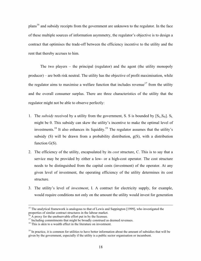
This contract structure may be illustrated by Figure 2 below.

Figure 2

The ρ(B,S) = 0 line is the iso-rent locus of the menu of contracts (reward-

commitment pairs) that a regulator can offer a utility. The locus is convex in S given

Assumption 1 and equation (9) above, through its interaction between p(.) and T(.), both of

which are functions of S.

4.2 The optimisation exercise

The optimisation exercise can be decomposed into two parts. In the first, the utility

chooses an investment rule that maps its optimal level of investment to the contract option

offered by the regulator (as outlined through its production function above). The second

part is the regulator’s optimisation exercise, where he incorporates this rule in its surplus

function, and offers a commitment-reward contract that optimises the total expected (utility

and regulator) surplus.

H

ρ (B,S) = 0

S* Commitment B

Subsidy S

Rew

ard

T

27

4.2.1 Case 1: Symmetric information

4.2.1.1 Case 1a: Perfect information

In the first case, with perfect information, the regulator’s decision problem has the

following characteristics. There is no adverse selection problem, as the regulator and utility

both know the level of subsidy that will be provided. The moral hazard problem still

remains, since the level of investment of the utility remains unknown to the regulator.

The regulator can calculate the level of investment that maximises total expected

surplus (the regulator’s and utility’s)27, which is:

I*(T) = argmax I {p(I)H – I} (10)

The regulator then announces a reward T = I*, if the utility delivers I*, and 0

otherwise. The utility also (weakly) prefers to deliver I*, so that the regulator’s optimal

outcome is ensured.

Substituting the utility’s chosen investment level (from (6) above) into (2),

T** = argmax T {p(I*(T))[H – T] + B} (11)

This means that for a utility that has limited amounts of expected subsidy, the

regulator can cap the rent to the utility by offering a reward T** that maximises the

regulator’s expected net return from production.

27 The regulator’s objective function is {p(I)[H-T] +B]; the licensee’s is {p(I)T – I – B}.

28

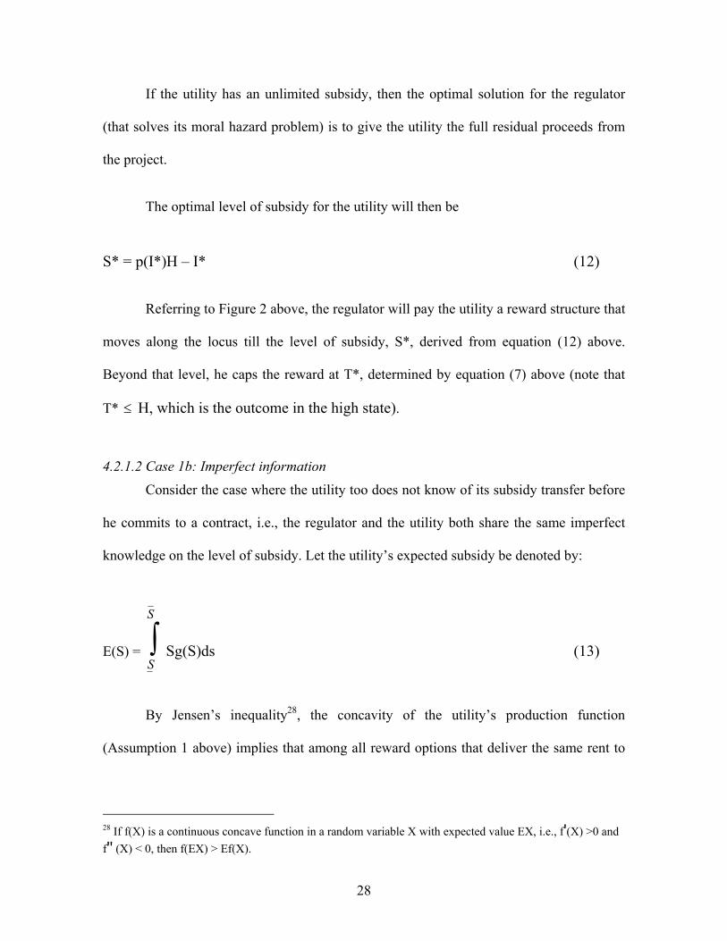
If the utility has an unlimited subsidy, then the optimal solution for the regulator

(that solves its moral hazard problem) is to give the utility the full residual proceeds from

the project.

The optimal level of subsidy for the utility will then be

S* = p(I*)H – I* (12)

Referring to Figure 2 above, the regulator will pay the utility a reward structure that

moves along the locus till the level of subsidy, S*, derived from equation (12) above.

Beyond that level, he caps the reward at T*, determined by equation (7) above (note that

T* ≤ H, which is the outcome in the high state).

4.2.1.2 Case 1b: Imperfect information

Consider the case where the utility too does not know of its subsidy transfer before

he commits to a contract, i.e., the regulator and the utility both share the same imperfect

knowledge on the level of subsidy. Let the utility’s expected subsidy be denoted by:

E(S) = ∫S

SSg(S)ds (13)

By Jensen’s inequality28, the concavity of the utility’s production function

(Assumption 1 above) implies that among all reward options that deliver the same rent to

28 If f(X) is a continuous concave function in a random variable X with expected value EX, i.e., f'(X) >0 and f'' (X) < 0, then f(EX) > Ef(X).

29

the utility, the regulator will prefer that which induces the same level of investment for all

realisations of the level of subsidy, i.e., at the expected level of the utility’s subsidy.

This is an even better outcome for the regulator than the symmetric perfect

information case. The regulator will only need to guarantee the utility an expected profit of

zero, rather than for each realisation of the level of subsidy. This allows the regulator to

implement a reward T that varies only with the utility’s expected subsidy, not with actual

realisations. This is a counter-intuitive result, since increased uncertainty actually results in

a better outcome for the regulator. This can be represented by Figure 3 below.

Figure 3

S1 E(S)

E(T)

T(E(S))

ρ (B,S) = 0

S2 Subsidy S

Rew

ard

T

30

4.2.2 Case 2: Asymmetric information

4.2.2.1 Case 2a: Utility’s costs are known to regulator.

Consider the setting where the regulator cannot observe the level of subsidy. He

offers the utility the reward-commitment pair {B(S), T(S)}. The regulator’s optimisation

problem is as follows29:

Max B(S),T(S) ∫S

S [ p{I(T(S))[H – T(S)] + B(S) ] g(S)dS (14)

Subject to

ρ (S) = T(S) – B(S) > 0 (14a)

Denote the integrand in Equation (10) as

WR(S) ≡ p[I(π (S))H – I(S)] – π(S) + B(S)

This is the regulator’s expected welfare when the utility’s realised subsidy is S.

Proposition 1: The solution to (14) has the following properties:

(i) B(S) = S, π'(S) > 0 and WR'(S) > 0 for all π(S) < S*.

(ii) ρ'(S) = 0, for all S ∈ [ ,S S ], i.e., ρ = ρc , a constant.

29 This is the standard regulatory problem of maximising expected consumer surplus.

31

(iii) ∫S

S[ {p'(I)H – 1}

dπdI – 1 ]g(S)ds ≤ 0 if ρc = 0, and = 0 if ρc > 0

Proof: See Appendix

Property (i) says that the regulator optimally induces the utility to deliver its entire

subsidy as a commitment whenever the investment level is below the surplus maximising

level, I*. If the regulator did not do this, the outcome would be Pareto inferior, since the

more generous the profit share that the utility could be rewarded with to compensate for its

larger commitment, the larger the expected surplus as a result of increased investment and

a larger expected payoff for the regulator.

To prevent the utility from concealing some of the subsidies that he gets, the

regulator must reduce the share of profits the utility is awarded when he makes a smaller

commitment. The utility might wish to understate the extent of his subsidy, hoping to

convince the regulator of the need to earn higher profit shares to offset the losses that he

would incur. The regulator responds by demanding a lower commitment level and

promising lower reward for success, the higher the utility claims the cost to be. This is a

counterintuitive result that is not usually a part of the regulatory toolkit. At the same time,

limiting profit shares as rewards is a conflicting requirement for the regulator: with both

players being risk neutral, pronounced profit sharing can alleviate the regulator’s moral

hazard concerns, but can simultaneously aggravate risk sharing concerns.

Property (ii) says that the regulator maintains a constant level of rent by increasing

the utility’s reward (share of profit). The selected rent level then determines the menu of

32

profit sharing arrangements, one for each level of realised subsidy. Why would the

regulator try to keep the utility on a constant rent loci? As seen from property (i) above, the

regulator induces the utility to part with his entire subsidy to realise the gains from higher

investments induced by higher rewards. But diminishing returns to profit sharing (Equation

(9) above) implies that increases in the utility’s share of realised profit induce larger

investment the smaller the initial share of profit. In other words, the regulator will

implement a more generous reward scheme than one required to compensate the utility for

making a larger commitment, only at low levels of rent of the latter.

How is this level of rent chosen? Property (iii) determines the level by balancing

the expected benefits and costs associated with any particular level of rent. A higher

threshold rent increases the level of investment put in by the utility, but also increases the

rent level afforded to it.

4.2.2.2 Case 2b: Utility’s costs are not known to regulator

The regulator’s optimisation problem in (14) is now:

Max B(.,C),T(.,C)

∫C

[ p{I(T(.,C))}[H - T(.,C)] + B(.,C) ] f(C)dC (15)

Subject to the standard set of constraints. (15a)

Proposition 2: The solution to (15) has the following properties:

(i) TC(C,S) > 0 for all C ∈ [ CC , ].

(ii) T(C ,S) = H.

33

(iii) If S < B , then their exists a C ∈ [ CC , ] such that TC(C,S) > 0 for all C ∈ [C , C ]

and T(C,S) = T(C ′ ,S) for all C ∈ [ C , C ].

(iv) If S1 < S2, and S1, S2 ∈ [ S , B ], then T(C,S1) > T(C,S2) > T(C, B ) for all C ∈ [ C ,

C ].

Proof: See Appendix

Property (i) and (ii) state that the utility’s rewards will strictly increase the lower

his costs, at all levels of subsidies. Property (iii) implies that if the utility has access to only

limited amounts of subsidy, the regulator will never reward him the full value of the

project. Doing this would afford the more efficient utilities’ super-normal rents30.

The regulator cannot ensure the ideal outcome of Case 1a, since any attempt to do

so would induce the low-cost utility to overstate his costs to secure the franchise for a

lower price (or demand a higher profit share). To prevent this, the regulator would award

him a lower reward, but correspondingly ask a lower level of commitment. A utility would

thereby secure a higher profit share, the lower his costs.

To induce the utility to provide the maximum effort, however, the utilities are still

provided a reward that is relatively large compared to the level of commitment. This

enables lower cost providers to enjoy rents, and because of these rents, low cost utilities

would have lesser incentives to overstate costs. Consequently, when the regulator does not

know the utility’s cost, he may forego full extraction of subsidies when the utility’s cost

structures are high in order to limit the rent to utilities when their cost levels are low.

30 The broad features of such contracts can be discerned in the regulation of private electricity distribution companies of the Orissa state in India. Despite the small subsidy amounts relative to the total turnover of the

34

4.2.2.3 Case 2c: Both the costs and subsidy amounts are not known to the regulator.

The regulator’s optimisation problem is as follows:

Max B(C,S),T(C,S) ∫C ∫S {p[I(T(C,S)) [H – T(C,S)] + B(C,S)} f(S)g(C) dCdS (16)

This is the standard regulatory problem of maximising expected consumer surplus.

Subject to:

ρ(S) = T(S) – B(S) ≥ 0 (16a)

B(C,S) ≥ 0 (16b)

Proposition 3: When a solution to (16) exists31, it can be implemented by a set of contracts

that have the following properties:

(i) For each C ∈ [C, C ], there exists an S (C) such that B(C,S) = S for all S ≤ S (C)

for which the utility operates and B(C,S) < S for all S ∈ [ S (C), S ].

(ii) (Cost pooling) For each S ∈ [ ,S S ], there exists some C (S) such that

S)T(C,S),B(C, = ),(Τ),, SC'SB(C' for all C, C' ∈ [ C (S), C ].

(iii) (Subsidy pooling) For each C ∈ [C, C ], S)T(C,S),B(C, = ),(Τ),, S'CS'B(C

for all S, S' ∈ [ S (C), S ].

companies (and to be provided only indirectly through World Bank support), the regulator imposed stringent loss reduction and other revenue collection targets. 31 Lewis and Sappington [2000] state that it can be shown that a solution to Proposition 3 exists when Assumption 2 holds and f(.) and g(.) are both uniform densities.

35

Figure 4 below shows iso-contract loci, which are pairs of costs and subsidies for

which the utility operates under the contract identified in the solution to Proposition 3.

These loci are characterised by a Leontief nature: the L shaped loci indicate that subsidies

and costs are perfectly complementary in determining the power of the incentive scheme

under which the utility operates. This implies that a more powerful reward structure will be

acceptable only to those utilities with both access to higher levels of subsidies and a lower

cost structure, but this will not be true generally of larger subsidies or lower costs alone.

The intuition for this becomes clearer with the help of an example, delineated below.

Figure 4

Suppose that the vertex of Figure 4 above corresponds to a cost level of $60 and a

subsidy level of $4.5 (the numbers are to be seen in conjunction with Table 5 below). The

kinked locus implies that at a cost of $60, the power of any scheme associated with subsidy

Rat

e of

retu

rn s

ubsi

dy

Cost per unit

$4.5

$60

36

over $4.5 remains the same and will fail to separate utilities with different cost

characteristics.

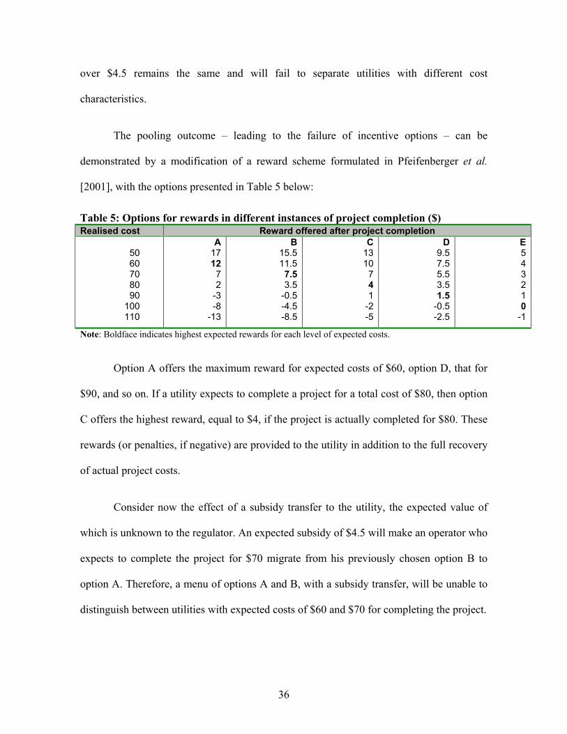
The pooling outcome – leading to the failure of incentive options – can be

demonstrated by a modification of a reward scheme formulated in Pfeifenberger et al.

[2001], with the options presented in Table 5 below:

Table 5: Options for rewards in different instances of project completion ($) Realised cost Reward offered after project completion

A B C D E 50 17 15.5 13 9.5 5

60 12 11.5 10 7.5 470 7 7.5 7 5.5 380 2 3.5 4 3.5 290 -3 -0.5 1 1.5 1

100 -8 -4.5 -2 -0.5 0110 -13 -8.5 -5 -2.5 -1

Note: Boldface indicates highest expected rewards for each level of expected costs.

Option A offers the maximum reward for expected costs of $60, option D, that for

$90, and so on. If a utility expects to complete a project for a total cost of $80, then option

C offers the highest reward, equal to $4, if the project is actually completed for $80. These

rewards (or penalties, if negative) are provided to the utility in addition to the full recovery

of actual project costs.

Consider now the effect of a subsidy transfer to the utility, the expected value of

which is unknown to the regulator. An expected subsidy of $4.5 will make an operator who

expects to complete the project for $70 migrate from his previously chosen option B to

option A. Therefore, a menu of options A and B, with a subsidy transfer, will be unable to

distinguish between utilities with expected costs of $60 and $70 for completing the project.

37

The larger the subsidy transfer, the less the power of the incentive scheme. An

expected subsidy of $8, for instance, will render options A, B and C unable to separate

utilities with expected cost levels of $60, $70 and $80. This can be depicted in Figure 4

above: for any given level of cost, a larger subsidy will reduce the power of the incentive

scheme. In other words, an iso-contract locus – i.e., a combination of rewards and

commitments – above and to the right of the one depicted in the figure will have lower

power.

The regulatory response to this specific environment involving multiple uncertainty

needs to be highlighted. Conventional theory argues that in this situation, full extraction of

the subsidy is not always optimal; “something” needs to be kept on the table for an

efficient utility. In the case investigated in this paper, however, this conclusion may be

reversed. When the levels of investment and the cost structure of the utility, together with

subsidy levels, are unknown to the regulator, it might not be optimal for the regulator to

allow the efficient utility rents. Higher levels of subsidies will be sought by the utility from

the government on the basis of higher stated costs. To discourage this, the regulator’s

response, for higher levels of (observed) subsidy would be to offer a smaller reward, with a

corresponding lower level of required commitment (implicitly to reduce costs). This is a

counter-intuitive outcome, since at first sight, it would seem better to offer the utility a

higher reward with a higher required commitment, in order to incentivise him to increase

investments. That, in fact, would have been a superior outcome in the absence of a subsidy

transfer. With subsidies and an inability of the regulator to distinguish between high and

low cost utilities, increases in up-front payments and rewards for success will generate rent

for the low-cost utility, given any specified level of subsidy. It is then rational for the

38

regulator to prohibit the utility from using the higher subsidy to secure a more powerful

reward structure, in order to limit its rents. Subsidies, then, are used as a signal by the

regulator to distinguish between high and low cost utilities, based on the assumption that

low-cost utilities will have less incentive to seek higher levels of subsidies and

consequently rewarded more.

The underlying intuitions of the rather lengthy and involved proof of Proposition 3

can be illustrated by a simple algebraic formulation. The following example also

demonstrates that the separating outcomes arising out of the contracts offered by regulators

under the previous cases with one degree of adverse selection asymmetry, breaks down

when there are two sources of information uncertainty. Consider an example of an

incentive scheme with linear reward and commitment structures:

Max {C,S,I}

C* Iγ (α

0C + β S) – I – (a

0C + b S) , 0 ≤ γ ≤ 1

Where C* is the actual cost and C and S are the declared cost and subsidy levels,

respectively. The first order conditions are as follows:

C* Iγ (α

0) - a

0 = 0 and C* Iγ (β) = 0

The solution being independent of C and S implies pooling. In other words, any

agent, whatever their declared C and S type, will choose the same I and opt for identical

incentive schemes. On the other hand, a quadratic reward commitment structure, of the

following form:

Max {C,S,I} C* I

γ (½) (α

0 C2 + β S2) – I – (½)(a

0 C2 + a

1 C + b S2)

39

will have as the first order conditions

C* Iγ (α

0)C - a

0 C + a

1 = 0 and C* I

γ (βS) = 0

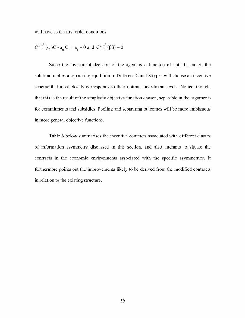
Since the investment decision of the agent is a function of both C and S, the

solution implies a separating equilibrium. Different C and S types will choose an incentive

scheme that most closely corresponds to their optimal investment levels. Notice, though,

that this is the result of the simplistic objective function chosen, separable in the arguments

for commitments and subsidies. Pooling and separating outcomes will be more ambiguous

in more general objective functions.

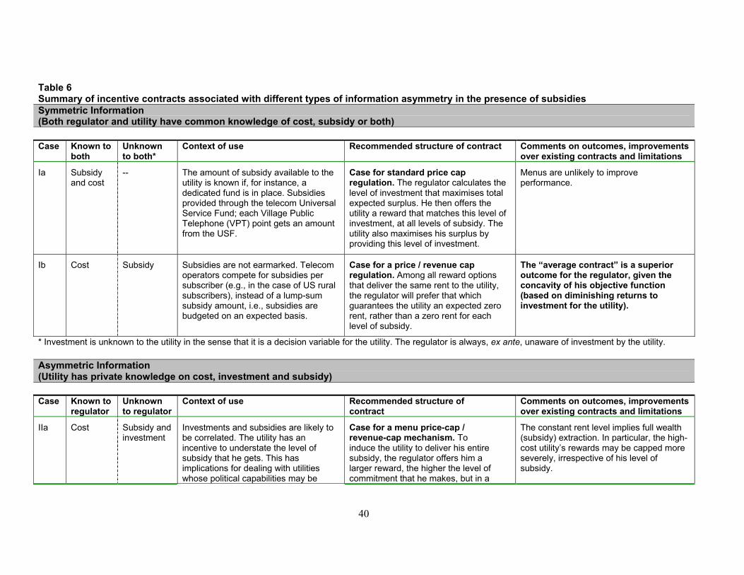
Table 6 below summarises the incentive contracts associated with different classes

of information asymmetry discussed in this section, and also attempts to situate the

contracts in the economic environments associated with the specific asymmetries. It

furthermore points out the improvements likely to be derived from the modified contracts

in relation to the existing structure.

40

Table 6 Summary of incentive contracts associated with different types of information asymmetry in the presence of subsidies Symmetric Information (Both regulator and utility have common knowledge of cost, subsidy or both) Case Known to

both Unknown to both*

Context of use Recommended structure of contract Comments on outcomes, improvements over existing contracts and limitations

Ia Subsidy and cost

-- The amount of subsidy available to the utility is known if, for instance, a dedicated fund is in place. Subsidies provided through the telecom Universal Service Fund; each Village Public Telephone (VPT) point gets an amount from the USF.

Case for standard price cap regulation. The regulator calculates the level of investment that maximises total expected surplus. He then offers the utility a reward that matches this level of investment, at all levels of subsidy. The utility also maximises his surplus by providing this level of investment.

Menus are unlikely to improve performance.

Ib Cost Subsidy Subsidies are not earmarked. Telecom operators compete for subsidies per subscriber (e.g., in the case of US rural subscribers), instead of a lump-sum subsidy amount, i.e., subsidies are budgeted on an expected basis.

Case for a price / revenue cap regulation. Among all reward options that deliver the same rent to the utility, the regulator will prefer that which guarantees the utility an expected zero rent, rather than a zero rent for each level of subsidy.

The “average contract” is a superior outcome for the regulator, given the concavity of his objective function (based on diminishing returns to investment for the utility).

* Investment is unknown to the utility in the sense that it is a decision variable for the utility. The regulator is always, ex ante, unaware of investment by the utility. Asymmetric Information (Utility has private knowledge on cost, investment and subsidy) Case Known to

regulator Unknown to regulator

Context of use Recommended structure of contract

Comments on outcomes, improvements over existing contracts and limitations

IIa Cost Subsidy and investment

Investments and subsidies are likely to be correlated. The utility has an incentive to understate the level of subsidy that he gets. This has implications for dealing with utilities whose political capabilities may be

Case for a menu price-cap / revenue-cap mechanism. To induce the utility to deliver his entire subsidy, the regulator offers him a larger reward, the higher the level of commitment that he makes, but in a

The constant rent level implies full wealth (subsidy) extraction. In particular, the high-cost utility’s rewards may be capped more severely, irrespective of his level of subsidy.

41

Case Known to regulator

Unknown to regulator

Context of use Recommended structure of contract

Comments on outcomes, improvements over existing contracts and limitations

higher than commercial ones. A situation here might be the case of power distribution subsidies. The utility, by disguising theft as agricultural consumption, can ask for larger subsidies.

manner that keeps his rent constant. Revelation about true subsidy levels can be incentivised through commitment levels, so that utility does not lose through higher subsidies.

To ensure that subsidies are used only for covering the tariff gap and not commercial losses, the regulator might insist on a commitment to meter agriculture consumption while allowing higher tariffs / lower loss reduction targets.

IIb Subsidy Cost and investment

Since the utility will have an incentive to overstate costs, to convince the regulator that project success is costly, the regulator’s optimal response will be to offer a smaller reward, and demanding a correspondingly smaller commitment, the larger the level of subsidy. This is particularly true of higher cost utilities. When the subsidy is limited, the regulator will not reward the utility the full value of the project.

Case for a menu subsidy cap. A commitment by the utility to a faster reduction in commercial losses will be matched by the regulator permitting a larger increase in tariffs. Full extraction of subsidy is not always optimal in this case, especially in the case of a high cost utility, in order to limit the rent that would accrue to a low-cost utility if he declares his costs to be high.

This case is especially relevant for case where the utility has access to an earmarked fund, but many contracts are being given to different utilities with widely varying cost structures.

IIc -- Investment, subsidy and cost

Multiple degrees of uncertainty leading to a regulator being unable to offer high / low power incentive contracts to different utilities.

Assuming that subsidies mimic the revenue realisation gap, a non-linear schedule of incentives that disallows a higher reward for higher commitment levels is the optimal response for the regulator.

The regulator will be unable to distinguish between operators of different efficiencies, and the incentive structures will result in pooling of utilities of varying efficiencies. A price or revenue cap type of incentive regulation is unlikely to be effective.

42

5. APPLICATION TO UTILITY REGULATION

This section assesses the relevance of the theoretical model presented in the paper for

evaluating the contracts that have hitherto been awarded, are being considered for award or are

likely to be awarded in the future, for utility services in India. Thus far, the most numbers of

contracts to private companies have been awarded in the power sector, and consequently, most of

our examples will be drawn from this sector32. Table 7 below is a schematic classification of

characteristics of infrastructure sectors designed to facilitate the customisation of menu contracts.

Table 7: Classification of sectors in congruence with model variables Subsidy Investment

Low

Medium

High

Low • Water & waste management contracts

• Power distribution

Medium • Industrial Water Supply

• Rural telecom and IT networks

• Public road transport

High • Power generation • Ports

• Urban transport

5.1 An application to contracts for power projects

Power generation projects in emerging markets offer the best illustration of the adherence

to (or deviation from) the principles of an optimal menu of contracts delineated in the previous

section. Most power projects in developing countries operate under long term Power Purchase

Agreements (PPAs) signed with the conceding authorities and not as merchant power plants (i.e,

selling directly into spot markets for electricity). Although many of these contracts have been

awarded through competitive bidding (that were designed to extract the rents inherent in

43

negotiated PPAs), the structure of the bids and associated informational asymmetries have been

thought to have left the conceding authorities at a disadvantage.

Information asymmetries are considerably aggravated when a project is large. There is a

bias in many developing countries towards “mega” power projects deriving from an instinctive

desire of attracting large amounts of private capital. This has led to a series of problems with large

IPPs in many developing and transitional countries ranging from Central Europe to Pakistan,

India, Indonesia and the Philippines.

The award of a contract to the Enron sponsored Dabhol Power Corporation (DPC) in India

is illustrative of the problems caused by a contract that is uniform and allows the agent to extract a

significant rent by leveraging on information asymmetries. The 2,184 MW, $2.8 bn project has an

overwhelmingly large take-or-pay structure33, which takes most of the risks away from the project.

The rate of return on equity that is factored into the tariff is approximately 30 percent, far too high

for the commensurate levels of risk that were to be borne by the sponsors. Although there are

commitments for DPC built into the 30 year Power Purchase Agreement (PPA), for instance on

heat rates, availability, ramp-up time to maximum power, etc., these are technical requirements. It

is now obvious that the excessively high rate of return – far beyond those justifiable by the extent

of risks normal in a developing nation – was ipso facto a subsidy given to the project34.

Contrast the problems with the instances of successful concessioning and commissioning

of gas operated power plants in many other emerging markets. The marked differences in these

32 The telecom sector is, of course, the most commercial, but, other than concessions for rural telephony, competition precluded the license award mechanisms that we deal with in this paper. 33 The variable cost per unit of power from the Dabhol plant operating at 90% PLF is 0.2 cents. 34 This is another example of implicit subsidies mentioned earlier in section 2.

44

experiences indicate a problem with not only the size of these projects, but also the degree of

implicit subsidy (in the form of revenue and other guarantees) that have been given.

The DPC contract also illustrates the other aspect of commitment that we have not

addressed in this paper – that of the principal’s35. Despite the signing of an “iron-clad” contract,

there have been continuing defaults by the contractual purchaser of the power, the Electricity

Board of the State of Maharashtra (MSEB). DPC was expected to sell to a bankrupt utility (ninety

percent of whose customers are subsidised), and the gap between the receipts of MSEB and the

contracted payments was to have been made up by the state and central government. Only a

fraction of these payments have materialised. Therefore, ex post, DPC, may feel justified in having

ex ante demanded a high risk premium!

The main lesson here is that the risks of setting up large projects in developing countries

often offset the occasional economies resulting from size. In sharp contrast to DPC is the case of a

216 MW gas-based power plant set up in Andhra Pradesh. The capital cost of this project is Rs

474 million per MW.

5.2 An illustration of a separating contract for a power distribution license

Penalties and incentives necessarily go together: if there are incentives to perform, there

must also be penalties for non-performance. However, instead of penalties, asymmetric

incentives, involving a financial downside as well as an upside is also likely to result in certain

performance characteristics. In some incentive schemes, such as the Kanpur Electricity Supply

35 The approach of our paper is, of course, different to that of the standard commitment literature. Our paper is a one-period contract without the dynamics of credibility of commitments inherent in a multi-period model.

45

Company’s (KESCO) privatisation bid in 1999-2000, the downside risk was greater than the

upside benefit in beating designated performance targets (Tadimalla [2000]).

A simple illustration of a separating contract may be a licensing exercise for a power

distribution company, where the utilities have a choice of opting for a concentrated (urban) zone

versus a consolidated (urban and rural combined) one. Assume that there are two types of utilities,

with the more efficient type (Utility 2) dominating the other. The figures in Tables 8a and 8b

below indicate the payoffs to these utilities from operating the distribution license for specially

configured zones. The figures in brackets represent the payoffs from the rural zones, which are

measures of subsidies provided to the utilities for operating in the rural areas (and which are a

component of the total payoffs of the utilities). Note that the payoff to utilities from the

consolidated zone is less than that from the concentrated zone and the subsidy combined, due to

the additional cost of integration of two different kinds of systems. It is this loss that makes it

optimal to separate the utilities in service provision in the concentrated and rural areas.

Table 8a: Payoffs to a utility from a distribution license (Case IIb) Consolidated zone

(concentrated + rural)Concentrated zone

Utility 1 700 (300) 500

Utility 2 1200 (300) 1000

Consider the simple case where the regulator knows the payoffs of the utility, but cannot

distinguish the efficiencies of the two utilities (corresponding to case IIb of Table 6 above). Let a

reserve price of 300 be set for the rural zone. Bidding in this structure ensures that Utility 2 gets

the license for the concentrated zone and Utility 1 will (as a residue) bid for the rural zone (having

to pay only as much of its supernormal profits). The payoff to the regulator increases in the case

where the utilities segregate themselves in serving the two zones, i.e., (i) if Utility 2 bids for the

46

consolidated zone (payoff to regulator is 1200) or (ii) Utility 2 bids for the concentrated zone and

Utility 1 for the rural zone, respectively (payoff to regulator is 1300).

Now consider the case (corresponding to case IIc) where the regulator is uncertain about

the subsidy transfer (Table 8b shows the regulator’s expectations of payoffs).

Table 8b: Expectations of regulator about payoffs to a utility (Case IIc) (a): E(S) > S (b): E(S) < S Consolidated

zone Concentrated

zoneConsolidated

zone Concentrated

zoneUtility 1 800 (400) 500 Utility 1 600 (200) 500

Utility 2 1300 (400) 1000 Utility 2 1100 (200) 1000

If the regulator believes the expected subsidy is 400, and sets a reserve price of 400 for the

rural zone, neither utility will bid for the rural zone. If, on the other hand, he expects the subsidy to

be 200, and sets this as the reserve price, Utility 2 will be indifferent between the zones (since he

obtains the same payoffs in both the zones) and a pooling equilibrium emerges (with the regulator

unable to separate the two utilities into the two zones), with Utility 1 being shut out and the payoff

to the regulator consequently less than under a separating equilibrium.

6. CONCLUSION

In an environment of multiple information asymmetry, regulatory contracts that give rise to

separating equilibria are a critical component in any exercise to simultaneously incentivise

efficient provision of services and extract rents from efficient service providers. A suitably

designed menu of contracts has been considered an incentive compatible means of achieving

separating equilibria. This paper investigates the properties of an optimal contract between a

regulator and utility in the context of utility investment, where the utility receives subsidies from

the government.

47

Subsidy transfers, besides increasing the information asymmetries, also serve to create a

distortion in utilities’ investment decisions through a “wealth” effect. This paper has attempted to

provide an analytical framework to formulate a mechanism of regulatory oversight of utilities

when large and uncertain subsidy transfers to the utilities from the government induces multiple

uncertainties between utilities and regulators. We show that in this situation of multiple adverse

selection and moral hazard, many of the standard menus of contracts designed as means of

information disclosure in an environment of more limited asymmetry results in nullifying much of

the power of standard incentive regulation and the ability of the offered contract to distinguish

between utilities. When the levels of subsidies, furthermore, are observed only imperfectly by the

regulator, this creates an incentive for the utility to demand higher rewards (larger revenue shares

or higher tariffs, etc.) from regulators.

The regulator can best motivate a utility, under these conditions, to make the optimal level

of investment by structuring a menu of rewards and commitments that are contingent on the

relevant source of uncertainty and will vary depending on the variable(s) that is (are) private

information to the utility. This implies that each individual utility concession has to be tailored,

and a “one size fits all” concession is not likely to be optimal, as a consequence, raising the

transaction costs of regulation.

There are three main conclusions from the paper. One, contract menus are the optimal

revelation mechanism in this environment. Two, many menus of the types that have been offered

by regulators to utilities are likely to fail in this objective under circumstances investigated in the

paper. Third, menus need to be tailored to address the relevant source of uncertainty.

48

These conclusions have significant implications for regulatory pricing in developing

countries, where tariff setting for utilities is done predominantly on a cost-plus basis. One is the

generally accepted conclusion that the mode of regulation needs to move away towards an

incentive based system like RPI-X. Second, and more importantly, in the particular case, when

multiple asymmetries are present, even the standard incentive regulatory schemes are unlikely to

achieve the desired results; regulatory schemes need to be tailored according to the specific

uncertainties that characterise the system. Since low-cost utilities would have an incentive to

overstate costs and thereby extract rents, the regulator should optimally devise a sliding scale

where lower cost utilities are allowed higher rents. In other words, higher declared cost structures

are penalised by being offered lower rewards. The Private Finance Initiative (PFI) contracts in the

UK broadly bears this out, since each contract (defining the investment and subsidy components

involved) has had to be tailored. Finally, in an environment when the information uncertainty is

symmetric, the model suggests that, by making an expected (in probability terms) reward scheme

deliver a superior outcome to individual schemes, that regulators not micro-manage decisions,

thereby buttressing the often heard recommendation for regulators to focus on “doable” actions.

49

References

Armstrong, M., 1999, “Optimal Regulation with unknown demand and cost functions”, Journal of Economic Theory, vol. 84, pp. 196-215. Armstrong, M. and D. E. M. Sappington, 2003, “Towards a unified treatment of adverse selection problems”, Discussion Paper, Nuffield College, November. Baker, B. and S. Tremolet, 2000, “Utility reform: Regulating quality standards to improve access for the poor”, World Bank Note No. 219, October. Baron, D. and R. Myerson, 1981, “Regulating a monopolist with unknown costs”, Econometrica, vol. 50(4), pp. 911-930. Bhattacharya, S. and U. R. Patel, 2001, “New regulatory institutions in India: White Knights or Trojan Horses?”, also forthcoming in volume of Conference Proceedings on Public Institutions in India: Performance and Design, Harvard University (revised May 2003). Bhattacharya, S. and U. R. Patel, 2003, “Markets, Regulatory Institutions, Competitiveness, and Reforms,” SCID, Stanford University, Working Paper No. 184, September. Boitani, A. and C. Cambini, 2002, “Incentive regulation of local public transport: The subsidy cap mechanism”, Working Paper, Universita Cattolica del Sacro Cuore, Milan, March. Crew, M. A. and P. R. Kleindorfer, 2000, “A critique of the theory of incentive regulation: Implications for the design of performance based regulation for postal service”, paper prepared for Rutgers University 13th Annual Western Conference on Competitive Challenge for Network Industries, Monterey, California, July. Crew, M. A. and P. R. Kleindorfer, 2002, “Regulatory economics: Twenty years of progress?”, Working Paper, University of Pennsylvania. de Moor, A. P. G., 1997, “Key issues in subsidy policies and strategies for reform”, UN Fourth Expert Group Meeting on Financial Issues. de Moor, A. P. G., 1998 “Perverse incentives: Subsidies and sustainable development”, Mimeo., Institute for Research on Public Expenditure, the Netherlands. Green, J. and J. Laffont, 1986, “Partially verifiable information and mechanism design”, Review of Economic Studies, vol. 53, 447-456. Guesnerie, R., P. Picard and P. Rey, 1989, “Adverse selection and moral hazard with risk-neutral agents”, European Economic Review, vol. 33(4), pp. 807-823.

50

Kay, J., 2003, “Are the increasingly frequent failures in electricity supply the result of privatisation and deregulation?”, Financial Times, October 1. Laffont, J-J. and J. Tirole, 1986, “Using cost observations to regulate firms”, Journal of Political Economy, vol. 94, pp. 614- . Laffont, J-J. and Tirole, J, 1993, Theory of incentives in procurement and regulation, MIT Press. Laffont, J-J. and D. Martimort, 2001, “The theory of incentives: The principal-agent model”, Princeton University Press. Lewis, T. and D. Sappington, 1988, “Regulating a monopolist with unknown demand and cost functions”, Rand Journal of Economics, vol. 19(3), pp. 438-457. Lewis, T. and D. E. M. Sappington, 1999, “Optimal contracting with private knowledge of wealth and ability”, Rand Journal of Economics, vol. 19, pp. 438-457. Lewis, T. and D. E. M. Sappington, 2000, “Motivating wealth-constrained actors”, American Economic Review, vol. 90(4), pp. 944-960. McAfee, R. P. and J. McMillan, 1988, “Multidimensional incentive compatibility and mechanism design”, Journal of Economic Theory, December, vol. 46, pp. 335-354. Page, F. H., Jr., 1992, “Optimal contracting mechanisms for principal agent problems with moral hazard and adverse selection”, Economic Theory, vol. 1, pp. 323-338. Pfeifenberger, J. P., P. R. Carpenter and P. C.Liu, 2001, “REx incentives: PBR choices that reflect firm’s performance expectations”, The Electricity Journal, November, vol. , pp. 44-51. Picard, P., 1987, “On the design of incentive schemes under moral hazard and adverse selection”, Journal of Public Economics, vol. 33, pp. 305-331. Planning Commission (India), 2002, “Annual Report on the working of State Electricity Boards and Electricity Departments”, April. (Also see earlier issues). Sappington, D. E. M., 1983, “Optimal regulation of a multi-product monopoly with unknown technological capabilities”, The Bell Journal of Economics, vol. 14(2), Autumn, pp. 453-463. Sappington, D. E. M., 1991, “Incentives in principal-agent Relationships”, Journal of Economic Perspectives, vol. 5 (2), pp. 45-66. Sappington, D. E. M. and D. Weisman, 1996, “Designing options in incentive regulation plans”, in Designing Incentive Regulation for the Telecommunications Industry, MIT Press.

51

Shirley, M., 1995, “Contracting: What works, what doesn’t and why”, from Bureaucrats in Business: the Economics and politics of Government Ownership, Oxford University Press for the World Bank. Shirley, M. and L. Colin Xu, 1997, “Information, incentives and commitment: An empirical analysis of contracts between government and state enterprises”, Discussion Draft, The World Bank. Tadimalla, S., 2000, “Privatisation of Kanpur Electricity Supply Company (KESCO): A case study”, Mimeo., Infrastructure Development Finance Company Limited, Mumbai. Weisman, D., 2000, “Regulatory moral hazard: Price caps and endogenous entry under the 1996 Telecommunications Act”, in Expanding competition in regulated industries, M. A. Crew (ed.), Kluwer.

52

APPENDIX Proof of Proposition 1. The regulator’s optimisation problem is as follows:

Max B(S),T(S) ∫S

{p[I(T(S))*[H - T(S)] + B(S)} g(S) dS (14)

This is the standard regulatory problem of maximising expected consumer surplus.

Subject to

ρ (S) = T(S) – B(S) > 0 (15)

Denote the integrand in Equation (10) as

WR(S) ≡ p[I(π (S))H – I(S) – π(S) + B(S)

Set up the Hamiltonian Λ = [WR(S)]g(S) + λ(S) ρ'(S) + µ(S)[S – B(S)] where ρ(S) = π(S) - B(S) is the state variable, λ(S) is the co-state variable. ρ'(S) and B(S) are control variables. Assume that the regulator’s objective function is concave in T() and B(). Necessary Conditions: p' [I(S)H – I(S)]

dBdI g(S) - µ(S) = 0 (A.2)

λ'(S) = [1 – {p'(I)H – 1}

dρdI

] g(S) (A.3)

λ(S) ρ'(S) = 0 (A.4) µ(S)[S – B(S)] = 0 (A.5) [S – B(S)] ≥ 0 (A.6)

53

Proof of Property (i) (A.2) implies that µ(S) > 0 when π(S) < S*. Together with this, (A.5) implies that B(S) = S for all S for which π(S) < S*

Proof of Property (ii) Note that S* has been defined previously in (12) as that level of subsidy for which the regulator maximises his surplus. λ(S)ρ(S) = λ(S)ρ(S) = 0; λ(S), λ(S) ≥ 0 (A.7) Proof by contradiction: Suppose ρ'(S) > 0 for all S. Then (A.4) implies that λ(S) = 0 for all S. (A.1a) Using (A.3), [p'(I)H – 1]

dρdI

– 1 ≡ Φ(S) = 0, for all S (A.8)

Φ'(S) = p''(I)H[

dρdI

ρ'(S) + dBdI

B'(S)]

+ [p'(I)H – 1] 2

2

dρ

Id [ρ'(S) + B'(S)] (A.9)

Recalling that p'(I) > 0 and p''(I) < 0, Property (i) then implies that B'(S) = 1. From the definition of h, (also see (2)),

h = dρdI

= dBdI

(A.10)

Therefore (A.9) implies

54

Φ'(S) = p''(I)H[h{ρ'(S) + 1}] + (p'(I)H – 1)[h'{ρ'(S) + 1}] (A.11) From (A.2), p'(I)H – 1 > 0. Also from (1), ρ' + 1 > 0. Therefore, if h' ≤ 0, then Φ'(S) < 0. This contradicts (A.8), since Φ(S) = 0, for all S. Therefore, ρ'(S) = 0 for all S.

In other words, the optimal contract for the regulator is to maintain a constant level of rent by increasing the utility’s reward just enough to offset the larger commitment that he makes. Each selected rent level determines a menu of rewards and commitments, which will be exactly the subsidy obtained by the utility, from (11).

Property (iii)

The optimal level of rent selected by the regulator is determined at the level that exactly balances the benefits and costs associated with the level of rent.

Recall from (A.1b) that ∫S

Sλ'(S) = 0 when ρ(S) > 0 for all S ∈ [S,S].

(A.3) then implies

∫S

S[1 – {p'(I)H – 1}

dρdI

] g(S)ds = 0

The Proof of Proposition 2 follows on similar lines.