incarceration length, employment, and …harris.princeton.edu/pubs/pdfs/494.pdf incarceration...
TRANSCRIPT

WORKING PAPER # 494 INDUSTRIAL RELATIONS SECTION PRINCETON UNIVERSITY AUGUST 2004 http://www.irs.princeton.edu/pubs/working_papers.html
INCARCERATION LENGTH, EMPLOYMENT, AND EARNINGS
Jeffrey R. Kling *
* Princeton University and National Bureau of Economic Research.
This paper revises and extends work previously circulated as “The Effect of Prison Sentence Length on the Subsequent Employment and Earnings of Criminal Defendants,” Woodrow Wilson School Economics Discussion Paper 208, February 1999. Assistance in data production was generously provided by Steve Schlesinger and Cathy Whitaker at the Administrative Office of the U.S. Courts, Dave Jones at the California Employment Development Department, John Scalia at the Bureau of Justice Statistics, Bill Sabol at the Urban Institute, William Bales, John L. Lewis, Brian Hays, and Stephanie Bontrager at the Florida Department of Corrections, Sue Burton at the Florida Department of Law Enforcement, and Duane Whitfield at the Florida Education and Training Placement Information Program. Thu Vu provided valuable research assistance. I benefited greatly from the advice of Joshua Angrist, Jerry Hausman, and Lawrence Katz. Helpful comments were also made by Daron Acemoglu, James Anderson, Marianne Bertrand, Shawn Bushway, Ken Fortson, Jane Garrison, Kara Kling, Alan Krueger, David Lee, Jeff Liebman, Mike Piore, Anne Piehl, Steve Pischke, Whitney Newey, John Tyler, Bruce Western, Bill Wheaton, and numerous seminar participants. This research was partially supported with grants from the National Science Foundation (9530182 and 9876337), the Alfred P. Sloan Foundation, and the Russell Sage Foundation. Additional support was provided by the Princeton Office of Population Research (NICHD 5P30-HD32030), and the Princeton Industrial Relations Section.
© 2004 by Jeffrey R. Kling. All rights reserved.

Princeton IRS Working Paper 494 August 2004
INCARCERATION LENGTH, EMPLOYMENT, AND EARNINGS
Jeffrey R. Kling
ABSTRACT Incarceration directly affects a significant and increasing share of Americans, and the lengths of new incarceration spells have increased dramatically in the past twenty years. Employment in the legitimate, mainstream economy is a key factor in the reintegration of former inmates into society after release. While considerable literature documents large adverse labor market consequences of going to prison, this paper provides the first evidence focusing directly on the effects of increases in incarceration length on the employment and earnings prospects of individuals after their release from prison. Data on inmates are from the state system in Florida and the federal system in California, linked to administrative records of quarterly earnings.
This paper utilizes a variety of research designs in an attempt to identify the causal effects of increases in incarceration length: controlling for observable factors, accounting for pre-spell differences in outcomes, and using instrumental variables for incarceration length based on randomly assigned judges with different sentencing propensities. The results show no consistent evidence of adverse labor market consequences of longer incarceration length using any of the analytical methods in either the state or federal data. Keywords: prison sentence length; labor market outcomes JEL classifications: J24; K42 Jeffrey R. Kling Department of Economics and Woodrow Wilson School Princeton University Princeton, NJ 08544 and NBER [email protected]

1
The fraction of the American population that has served time in state and federal prisons
is large, and has been growing over time. As of the end of 2001, three percent of all U.S. adults
had been incarcerated at some point in their lives. Among African-American males, 17 percent
had ever been incarcerated, up from nine percent in 1974. If current incarceration rates remain
unchanged, 32 percent of African-American males born in 2001 will go to prison at some point
during their lifetimes.1
Concurrent with the increased fraction of individuals ever imprisoned has been the
increased duration of incarceration. For example, the federal Sentencing Reform Act, which was
implemented in 1987, increased the lengths of the maximum sentences that individuals could
expect to serve for various offenses, eliminated probation, and decreased the potential for good
behavior to reduce the amount of time served -- effectively doubling average time served in
prison.2 Although states vary widely in their incarceration policies, many have adopted truth-in-
sentencing laws that involve requirements similar to federal guidelines that a new prison
admission serve at least 85 percent of the sentence.3 From 1987 to 1996, time served in state
prisons increased by 40 percent or more, depending upon the offense.4
1 Estimates of the prevalence of imprisonment are from Bonczar (2003). 2 In 1986, the average sentence of an offender entering federal prison was 39 months and the average percentage of the sentence actually served was 58 percent, for an average time to be served of 21 months. By 1993, the average sentence was 53 months, the percentage of sentence served was 85 percent, and the average time to be served had more than doubled to 45 months. Data are from Sabol and McGready (1999). 3 For example, Florida implemented sentencing guidelines in 1994 that increased the proportion of the sentence to be served in prison, and revised these guidelines again in 1995 to add stiffer penalties for various offenses. Nationally, by 1997 two-thirds of violent offenders were in states requiring them to serve at least 85 percent of the sentence; as a baseline for comparison, violent offenders released from prison in 1996 had served about half of their sentences on average (Ditton and Wilson 1999). 4 Blumstein and Beck (1999) estimate time served for murder, robbery, assault, burglary, and sexual assault; they find that for each of these offenses, time served increased substantially in the early 1990s. As the authors note, their methods underestimate time served when prison admissions per arrest rise over time, as they did over this time period. Lynch and Sabol (2001) report that the mean time served to first release in state prisons increased from 21 months in 1993 to 28 months in 1998.

2
The number of prisoners released each year has increased threefold in the past two
decades, to over half a million per year.5 A key element of successful reintegration into society
after release is believed to be employment in the legitimate mainstream economy.6 Most
previous research about the effects of incarceration on labor market outcomes has found large
effects of incarceration, but has focused on the effect of serving some time in jail or prison,
versus serving no time.7 Other research has focused on the effects of arrests and convictions on
labor market outcomes.8 Relatively little is known about the effects of incarceration length on
labor market outcomes, although some related work suggests substantial negative effects on
earnings.9 Yet, sentencing commissions need information on subsequent labor market impacts to
make informed decisions about the total costs of changes in incarceration length, since effects on
employment and earnings would directly affect individuals, their families (through family
income and child support), and government tax revenue long after the incarceration spells 5 Data are from 1980 to 1999, from Lynch and Sabol (2001). 6 For example, Petersilia writes, “Employment remains one of the most important vehicles for hastening offender reintegration ...” (2003, p.40). For general discussion of prisoner reentry issues, see Reentry Policy Council (2004), and Travis, Solomon, and Waul (2001). 7 For a review, see Western, Kling, and Weiman (2001). Waldfogel (1994b) and Freeman (1992) find large effects of having been incarcerated on income and employment, respectively, with decreases on the order of 25 percent for those who served jail or prison terms. Western (2002) finds large effects on having been incarcerated on both wages (10 to 20 percent) and wage growth (30 percent) of young men. 8 For reviews of the literature on crime and labor markets, see Freeman (1999) and Bushway and Reuter (2002). Waldfogel (1994b) finds small negative effects on income for conviction in federal crimes that do not involve a breach of trust, and moderately larger negative effects when a breach of trust is involved. Most previous research has studied young men. Grogger (1995) presents results on the temporary negative impact of arrests. Grogger (1995) and Freeman (1992) both find small negative effects for conviction. Nagin and Waldfogel (1995) actually find positive effects of conviction on youth’s later earnings, which they interpret as an indication that convicted youths are taking jobs in spot labor markets that have higher initial wages but lower long-term earnings trajectories. 9 Needels (1996) examined how the percentage of time offenders were incarcerated over an eight-year period (1976-1983) affected labor market outcomes during the subsequent nine-year period. The sample members were all inmates originally released in 1976 as part of the Transitional Aid Research Project in Georgia, and the time served measures the extent of recidivism rather than differences in initial lengths of incarceration spells. The labor market outcome data, available from 1983-1991, was from the Unemployment Insurance system in Georgia. Needels found no significant effect for employment, and found that an additional year of incarceration reduced total earnings from 1983-1991 by about 12 percent. Much of this reduction is associated with the percentage of time incarcerated from 1983-1991. Lott (1992a) found no significant relationship between prison sentence length and the difference in income before and after conviction for federal drug offenders. Lott (1992b) found very large effects of prison sentence length on earnings for federal fraud and embezzlement offenders, where a one-month increase in sentence length is associated with a decline in income of 5.5 to 32 percent, depending upon the specification. These specifications constrained the effect of serving any prison time (i.e., the first month) and the effect of additional months to be the same.

3
themselves have ended. This paper provides the first evidence that focuses directly on the effect
of additional incarceration length on employment and earnings after release from prison.
Any credible assessment of the effects of incarceration length must address the analytical
problem that prison sentences are related to offense severity and criminal history. A simple
comparison of groups serving one year versus four years in prison does not represent the
counterfactual of interest -- what would have happened to the group serving one year if they had
instead served four years. In this paper I use various research designs to approximate this
counterfactual that control for observable factors, account for pre-existing differences in labor
market prospects, and rely on variation within sentences that is not related to individual
characteristics -- using randomly assigned judges to form instrumental variables for sentence
length.10
These research designs require rich panels of data about offenders and their labor market
outcomes. Collaboration with numerous government agencies produced data for this study from
the state prison system in Florida and the federal judicial system in California that links
information about offender characteristics, incarceration experiences, and about ten years of
earnings data reported by employers in these two states through the Unemployment Insurance
(UI) system.
Several mechanisms have been proposed that could in theory link longer incarceration to
large negative effects on labor market outcomes. Most prominent are those involving worker
productivity; there could be negative effects of lost work experience and a more general
deterioration in human capital as skills may go unused during incarceration. Another possibility
is that criminal background and its associated stigma may be more salient to employers after
longer incarceration spells, although this mechanism may work primarily through conviction
10 For a general discussion of these types of research designs, see Angrist and Krueger (1999).

4
rather than incarceration length. Alternatively, longer incarceration length may allow the
criminal justice system to reduce recidivism and encourage work through rehabilitative programs
or post-release supervision. And direct social contacts with non-incarcerated criminal peers in
the community may erode during prison, making legitimate work relatively more attractive after
release from a longer incarceration spell.
Both the more prominent theoretical arguments and the previous related literature suggest
a null hypothesis of a large negative effect of incarceration length on labor market outcomes. In
brief, however, I find in this analysis that there is no substantial evidence of a negative effect of
incarceration length on employment or earnings. In the medium term, seven to nine years after
incarceration spells began, the effect of incarceration length on labor market outcomes is
negligible. In the short term, one to two years after release, longer incarceration spells are
associated with higher employment and earnings -- a finding which is largely explained by
differences in offender characteristics and by incarceration conditions, such as participation in
work release programs. While no single analytical method or data source provides irrefutable
evidence, the use of multiple methods and data sources in this paper helps corroborate these
findings.
The remainder of this paper is organized into five sections. Section one develops a
conceptual framework for interpreting results. Analytical methods are presented in section two.
Section three describes the data. Results are given in section four, and a discussion of
mechanisms driving the results is in section five. Section six concludes.
1. Conceptual framework
Various mechanisms through which an increase in incarceration length may affect labor
market outcomes are reviewed in this section, with a focus on identifying testable implications.
5
The first part examines mechanisms suggesting negative effects, and the second part examines
mechanisms suggesting positive effects.
A. Mechanisms suggesting negative effects of longer incarceration
One straightforward process is the loss of potential work experience while incarcerated.11
The importance of this mechanism depends upon the profile of returns to experience and the
location of inmates along that profile. Although the returns to experience appear to be
substantial for low-skilled workers in general (Gladden and Taber 2002), wage growth for
individuals after incarceration spells appears to be especially low (Western 2002). I examine this
process by estimating an earnings-experience profile and examining the distribution of potential
experience for inmates after the incarceration spell.12
Human capital may depreciate more if incarceration spells are longer. For example,
information technology may rapidly advance, and inmates may return to the labor market with
skills that are outdated. Inmates may instead return to spot labor markets with low returns to
skill (Nagin and Waldfogel 1995). If longer incarceration increases the chances of being more
suited for only unskilled, lower-paying work after release, then I hypothesize that the effects of
longer incarceration will be more negative for subgroups that had more education and higher
earnings prior to incarceration.
It is possible that effects of longer incarceration could manifest themselves through
stigma, if long spells of non-employment while in prison are more observable to employers.
However, previous research (e.g., Waldfogel 1994a) has emphasized the effect of stigma from
11 For example, loss of civilian work experience while in the military is cited by Angrist (1990) as a likely explanation for the 15 percent earnings loss experienced by white Vietnam veterans in comparison to non-veterans with similar risk of draft induction. 12 Specifically, I project forward seven years after the spell began, which is a time period that is observable in the data used in this paper, to forecast the average return to experience when the distribution of experience looks as it does in the post-incarceration period.

6
conviction itself rather than incarceration length, and criminal background checks are becoming
increasingly inexpensive and are being more widely used by employers (Holzer, Raphael, and
Stoll 2003). To the extent that there is a stigma effect associated with longer incarceration, I
hypothesize that it will be associated with groups that employers have less prior expectation of
being involved in criminal activity. For example, if many employers believe all young black
males are likely criminals, then the increased gap in work history from a longer incarceration
spell is unlikely to have much additional signal value. If this stigma process is operating, I
hypothesize that the effect of incarceration length will be less evident among minorities and
more evident among whites. I also speculate that the salience to employers of an additional year
of incarceration will be greatest for those with no criminal history prior to the spell, so I examine
effects for subgroups according to criminal history.
B. Mechanisms suggesting positive effects of longer incarceration
Longer incarceration spells could be associated with less recidivism -- specifically, a
lower probability of returning to prison.13 Even if the rate of employment among the non-
incarcerated were the same for all groups, for example, lower recidivism for those having served
longer incarceration spells could generate higher employment rates when looking at the
population of all former inmates (including recidivists and non-recidivists). In order to ascertain
the potential importance of this mechanism, in the analysis I directly examine the probability of
being in prison several years after the incarceration spell began. I also examine models in which
13 This could occur if a longer incarceration spell raised the expected costs of future punishment after release. Alternatively, if there were a constant probability (regardless of spell length) in each month after release of having a job in that month and of returning to a long prison term, then those released earlier would have a greater number of months where they would be at-risk for returning to prison for a long spell while the employment rates among the non-incarcerated would be equal across incarceration lengths when observing outcomes a certain length of time after the incarceration spell began.

7
labor market outcomes are treated as randomly-censored when an individual is in prison, in order
to focus on individuals in the mainstream labor market itself.
A separate mechanism that could lead to improved labor market outcomes would be
participation in academic, vocational, substance abuse treatment, or work release programs while
in prison that could increase employment capacity. Reviews of the literature on program
effectiveness do not for the most part suggest large effects (Wilson et al. 2000), and analysis of
the GED education program in Florida prisons does not suggest that any effects would be evident
as long as seven years after the incarceration spell began (Tyler and Kling 2004). However,
some programs may be effective and a longer stay in prison may increase the chances of program
participation. I examine the extent to which participation is associated with incarceration length,
and also include controls for program participation in model estimation.
Another process through which the criminal justice system itself may have a direct effect
of increasing subsequent employment and earnings is through post-release supervision. If the
terms of probation require an individual to be working with the possible sanction of being
returned to prison if employment is not found, employment rates may be quite high during
supervision but may not persist after the threat of sanction is removed. If a prison term of three
years plus probation were instead four years plus probation, then the probation itself could still
be in effect (and be having a greater impact on labor market outcomes) at a later point in time
when outcomes are measured. I examine this process by comparing the incarceration length
effects of subgroups of offenders with and without post-release supervision connected to their
original spells.
An indirect process through which longer incarceration could increase legitimate
employment and earnings is by reducing opportunities for illegitimate income, thereby making
legitimate work relatively more attractive. For example, longer incarceration spells could cause

8
social connections with criminal confederates to atrophy, making criminal activity more difficult.
This may be particularly true when non-incarcerated criminal peers are aging and reducing their
own levels criminal activity (Sampson and Laub 2003). When an incarcerated individual returns
home, it may be increasingly less feasible to return to previous patterns of behavior, and hence
more attractive to go into mainstream work. Because social interactions are particularly
important for certain types of offenses, such as drug crimes (Anderson 1990), I examine
subgroups by offense type. Since the change in peer activity with age is greatest for younger
individuals, I hypothesize that this mechanism connecting longer incarceration to better labor
market outcomes is more relevant for individuals who are younger at the onset of their spells,
and I therefore examine subgroups by age.
2. Analytical Methods
As a baseline for comparison, I first examine the simple association between
incarceration length and labor market outcomes such as employment and earnings. Let Y denote
the outcome and S denote the incarceration spell length, and let the subscript i refer to an
individual. An ordinary least squares (OLS) regression of this relationship is in equation (1).
(1) 11 iii SY εγ +=
The coefficient γ1 from this model is a convenient summary measure, interpreted as the
association of one additional year of incarceration with the outcome. The outcomes I use, such
as the individual’s average quarterly earnings, are defined for all individuals at a specified
amount of time relative to the incarceration spell. In order to account for differences in the types
of individuals serving shorter and longer prison terms, the remainder of this section provides four
approaches that enrich this simple model.

9
A. Controlling for observable factors
The first research design, presented in equation (2), includes covariates to adjust for
observable differences in individual characteristics (X) that may be correlated with both
incarceration length and labor market outcomes.
(2) 222 iiii XSY εβγ ++=
Estimates of the coefficient γ2 from this model represent the association of an additional year of
incarceration with outcomes, conditional on having the same individual characteristics. The
adequacy of only including S linearly is assessed by comparisons to models that include more
flexible functional forms of S.
B. Controlling for estimated pre-existing differences
Even among individuals with similar individual characteristics, it may be the case that
outcomes prior to the incarceration spell were associated with incarceration length. Intuitively, if
the association between future incarceration length and the pre-spell outcome is the same as
between incarceration length and the post-spell outcome, we can reasonably conclude that the
post-spell association is due to pre-existing differences and not an effect of the incarceration
spell itself. This is conceptually similar to a difference-in-differences research design, except that
a linear slope coefficient, rather than a difference between two group means, is being compared
in two time periods.
For the California data used in this paper, the sample size with observations on both pre-
and post-spell outcomes for the same individuals is too small for useful analysis. In order to
estimate the extent of any pre-existing differences, I impose a modeling assumption that the
association between incarceration length and pre-spell outcomes is stable over time. Under this
assumption, data on later cohorts of inmates (who have data available on pre-spell outcomes but

10
not post-spell outcomes) can be used in conjunction with data on earlier cohorts (who only have
post-spell outcomes) to estimate the extent of pre-existing differences.14 For equation (3), the
data include individuals who either only have post-spell outcomes or only have pre-spell
outcomes, with one observation per individual. S is the length of the incarceration spell (or the
upcoming incarceration spell, for individuals with pre-spell outcomes). Let D be an indicator for
former inmates with observed post-spell outcomes, where DiSi is the interaction of D and S for
each individual and D is also included in X.
(3) 3303130 iiiiii XSDSY εβγγ +++=
The coefficient of interest is γ31, which is the estimated association of incarceration length with
the outcome after the incarceration spell, subtracting the association estimated from data on
outcomes prior to a spell. Equivalently, γ31 is the effect of incarceration length on the outcome
after controlling for estimated pre-existing differences.
C. Controlling for actual pre-existing differences
The Florida system data have more extensive information on outcomes both before and
after incarceration spells for the same individuals, permitting a research design based on the
same intuition as just discussed, but employing actual pre-existing differences. The modeling
assumption used here is that the observed association of incarceration length with the level of the
outcome prior to the spell represents a pre-existing difference that would have persisted over
14 Note that since this assumption is about the slope of the association between incarceration length and outcomes, the model is not affected by an intercept shift in length over time (e.g., all sentences six months longer, for similar groups of offenders), but is affected by a slope shift (e.g., all sentences twice as long). To the extent that there are pre-existing differences and spell lengths increased by a multiplicative factor over time, equation (3) will over-estimate the magnitude of the incarceration length coefficient when the pre- and post-spell associations have the same sign. In practice, the magnitude of pre-existing differences appears to be small.

11
time.15 Denote ∆Y as the change in the outcome for an individual before and after the
incarceration spell, as shown in equation (4).
(4) 444 iiii XSY εβγ ++=∆
The coefficient γ4 is the effect of incarceration length on the change in the outcome or,
equivalently, on the level of the outcome after controlling for pre-existing differences. When X
is not included in equation (4), estimation is identical to an individual fixed effect model.
Inclusion of X controls for individual characteristics associated with changes in the outcome that
may also be correlated with incarceration length.
D. Instrumental variables
As an alternative strategy for estimating the effect of incarceration length on employment
and earnings, the judge who is assigned to the case can be used as an instrumental variable.
Judge assignments are available in the California data, and the random assignment of judges to
cases in California makes this an attractive instrument. Intuitively, this research design
compares groups of otherwise similar individuals who have shorter or longer prison sentences
because their cases were randomly assigned to judges that showed different levels of leniency in
sentencing. Equation (5) is used to estimate the effect on prison sentence length of the judge (Z)
assigned to the case, where cases are subscripted by j.16 A set of indicator variables for calendar
quarter in each district office (Q) is included to account for the fact that assignment of cases to
judges is randomly determined conditional on the date and location of case filing. 15 For some outcomes, such as earnings, it turns out that the pre- and post-incarceration levels differ substantially, making the assumption of a constant individual effect less plausible. However, it also turns out that incarceration length has little association with pre-incarceration outcome levels, making estimation of the coefficient of interest insensitive to this assumption. 16 In the California data, 48 percent of cases have multiple defendants. In order to reduce the sampling variability that would result from randomly selecting one defendant per case, equation (5) is estimated at the case level, averaging the prison sentences of multiple defendants with the same docket number. For the .6 percent of all cases in which all defendants were not assigned in the same calendar quarter to the same judge, one defendant was randomly selected and all defendants with the same judge and filing quarter were aggregated to represent the case.

12
(5) jjjj QZS ηθπ ++=
I use the parameter estimate π̂ from equation (5) to construct the instrumental variable π̂Z based
on the randomly assigned judge. This instrument is assumed to affect labor market outcomes
through incarceration length. I then use two-stage least squares estimation of equation (2) to
estimate the effect of incarceration length, with S as the endogenous variable and π̂Z as the
excluded instrument. This research design requires information on all cases assigned to judges,
including those not resulting in any prison time.
3. Data
The data used in this paper come from the administrative records of the state prison
system in Florida and the federal judicial system in California, each linked to state administrative
records about quarterly earnings. Nationally, in June 2003 there were 1.2 million inmates in
state prisons, 690,000 inmates in local jails, and 160,000 inmates in federal prisons (Harrison and
Karberg 2003). Roughly speaking, prisons are used in the U.S. for longer sentences (often at
least a year), while local jails are used for shorter sentences. Although most inmates are in state
systems, the federal system handles cases that directly involve the federal government and other
cases within federal jurisdiction.17 Florida and California were selected because of their large
prison populations, good data quality, and knowledgeable agency staff with genuine interest in
supporting research -- and, in the case of California, because of the availability of data on
complete caseloads randomly assigned to judges that could be linked to earnings records.
17 For example, an offense involving interstate postal fraud would be a federal case, as well as some offenses such as drug crime which the U.S. Congress has designated as potentially being within federal jurisdiction -- depending on the circumstances of the case (such as involvement of a federal officer, proximity to a federal building, etc.) and the priorities of prosecutors.

13
The Florida data were produced for this study in collaboration with the Florida
Department of Corrections (FLDOC). The data were compiled by linking separate FLDOC files
on correctional institution admission and release dates, jail credits, admission file demographics
(filling in missing data with subsequent monthly status files), reception center test scores, and
correctional institution disciplinary reports. Social Security Numbers (SSNs) from admission
files were verified by the Social Security Administration (SSA) using their Employment
Verification Service, matching names, birthdates, and race to SSA records of SSNs. The Florida
Education and Training Placement Information Program matched quarterly earnings data for
1993:3 through 2002:1 from the UI system to the FLDOC data. The Florida Department of Law
Enforcement provided arrest records.
The California data were produced under special confidential data-sharing agreements
with the Administrative Office of the U.S. Courts (for data on terminated federal cases with
individual and judge identifiers), California pre-trial services agencies (for demographic data and
SSNs), and the California Employment Development Department (for quarterly UI data from
1987:2 to 1997:1, linked by SSN).18
Descriptive statistics for these data are shown in Table 1. The first two columns show
characteristics of the Florida prisoners in the data for the models in equations (1) - (4).19 The
sample of inmates in column one began their incarceration spells in the calendar quarters 1994:3-
18 Because the sentencing data did not contain unique individual identifiers, the sentencing data were linked to pre-trial services data using probabilistic matching techniques relying upon non-unique identifiers of name, date, and offense type. In a pilot study of Massachusetts cases that did have unique identifiers, the matching logic and clerical review identified approximately 98 percent of all true matches with only .15 percent false matches. Despite this success, SSNs and demographic information were not collected in all years for each California district, resulting in a loss of 42 percent of the potential sample from 1983-94. A further 15 percent of the sample, which appear to be mainly immigrants, did not report SSNs. These data are collected prior to the assignment of a judge to the case, and reporting lapses appear to be independent of judge assignment. 19 Only new commitments to prison are used, not spells of incarceration that began in this period due to return to prison for violation of post-release conditions. The sample is also limited to those reporting they were U.S. citizens and Florida residents at the time of arrest and to those released to a Florida destination in order to reduce the influence of out-of-state mobility on the results.

14
1995:1. Given the available labor market outcome data, they are observed for four quarters prior
to incarceration and 28 quarters after the incarceration spell began. In order to examine medium-
term outcomes where all inmates have been released for at least two years, the analysis is limited
to those with incarceration spells of no more than 4.5 years. I further limit the analysis to spells
of at least six months, since nearly all shorter incarceration spells in Florida take place in local
jails and not in the state prison system. This sample of incarceration lengths represents about 80
percent of all individuals committed to prison.20 The sample used to analyze effects of
incarceration length shortly after release during the same period of calendar time is described in
column two, including releases in 1999:1-1999:3. This sample is slightly older, due to the
restriction for subsequent analysis that all members of this sample be ages 25-64 two and a half
years after release, but is otherwise quite similar to that in column one.
There are two main analytical samples based on California data. The third column of
Table 1 describes a sample constructed to parallel that for Florida in column one, with expected
incarceration spells of .5 - 4.5 years; actual time served is not observed in the California data, so
the expected spell length is based on the sentence length and historical averages of proportion of
time served published by the U.S. Department of Justice (1996). The fourth column describes
the data used to estimate the instrumental variables model, which includes all cases that were
randomly assigned to judges and have valid earnings data nine years after case filing. Although
19 percent of these inmates were expected to serve more than 4.5 years, 97 percent of the sample
was expected to have been released within nine years after their incarceration spell began. Since
this sample is used in the analysis to assess labor market outcomes nine years after case filing,
20 For the cohort incarcerated 1994:3 - 1995:1, 1.5 percent served less than 6 months and 17.5 percent served more than 4.5 years.

15
the three percent of the sample with expected spell lengths of more than nine years were top-
coded at nine years.
In terms of demographic characteristics, all of these samples are largely male. The
majority of the Florida sample is African-American, while the California samples have relatively
more whites, Hispanics, and other races. The Florida sample is younger, less-educated, has a
more extensive criminal history, and has more violent offenders; in these respects, the Florida
sample is similar to inmate populations in other state systems -- all of which tend to differ
substantially from the federal system (Harlow 1994). Florida is also fairly representative of
other states in terms of the race and ethnicity of offenders.21
For simplicity, the quarterly earnings data in this table and in subsequent regression
analyses consist of a single summary measure of pre-spell labor market outcomes for each
individual, averaging over three calendar quarters to reduce transitory variability.22 Similarly,
post-spell outcomes are the averages over three quarters.23 Quarterly earnings are adjusted to
2002 real dollars based on the seasonally-adjusted national Consumer Price Index (CPI), and are
top-coded at ten times the 2002 poverty rate ($23,398 per quarter). The analysis focuses on three
outcomes: fraction of quarters with any positive earnings, fraction of quarters with earnings
above the 2002 poverty threshold ($9359 per year, or $2340 per quarter), and average quarterly
earnings including zeros.
21 Note that the distribution of Hispanic inmates is highly skewed among states, with two-thirds of incarcerated Hispanics in California, Texas, and New York (which only have one-third of the overall prison population among them); Florida and other states have a much lower proportion of Hispanic inmates (Harrison 2002). 22 In column one, pre-spell outcomes are the average of the 2nd, 3rd, and 4th quarters prior to the incarceration spell. In column two, pre-spell outcomes are the average of the 22nd, 21st, and 20th quarters prior to release. 23 In column one, post-spell outcomes are the average of the 26th, 27th, and 28th quarters after the incarceration spell. In column two, post-spell outcomes are the average of the 8th, 9th, and 10th quarters after release.

16
The pre- and post-spell employment and earnings rates from the administrative data are
very low in both states, and similar to those of inmate populations in several other states.24 The
average fraction with positive earnings in the administrative earnings data for Florida one year
prior to the incarceration spell was only about one-third. However, nearly two-thirds of the
Florida sample self-reported that they were employed at the time of arrest. There are several
possible reasons for this discrepancy, including employment that was out of state, employment in
jobs not covered by UI, and false reporting.
In analyses of the Current Population Survey (CPS) from 1993 and 2000, weighted to
reflect the gender, race, education, and age distribution of the Florida inmates, I find that the self-
reported pre-spell inmate employment rate of .65 is very similar to the employment rate
nationally for a group with these demographics -- suggesting that the self-reported employment
rates of inmates may not be strongly biased by false reporting. In order to assess the proportion
of uncovered jobs for individuals with the demographics of inmates, I used the CPS April 1993
benefit supplement to calculate the fraction of those employed in the survey week whose
employers withhold Social Security from their paychecks as a proxy for being in a job covered
by UI. This analysis suggests that about one quarter of those with demographics like inmates
who report themselves as employed are working in jobs not covered by UI. Since the only
common characteristics in the inmate sample and CPS sample are gender, race, education, and
age, the CPS fraction with uncovered jobs is likely an underestimate for the true rate in the more
disadvantaged inmate population. But conservatively speaking, I conclude that uncovered jobs
explain at least half of the gap between the self-reports and administrative reports of employment
in these data.
24 See Needels (1996) for Georgia, Sabol (2004) for Ohio, and Pettit and Lyons (2002) for Washington state.

17
In studies using state UI data to measure employment and earnings, there are undoubtedly
some individuals employed out-of-state, and the fraction of uncovered legitimate employment in
these data on inmates, for example, appears quite substantial. In other research on job training
programs, Kornfeld and Bloom (1999) find that self-reported employment and earnings for adult
men are higher than UI reports, with the additional difference apparently due mainly to
uncovered jobs rather than out-of-state jobs.25 Their evaluation of training through the Job
Training Partnership Act, focusing on a different but also disadvantaged population, did find that
the differences between the treatment and control groups were similar for survey and UI
employment rates, even though the levels differed. This provides some evidence that between-
group differences in UI data can be quite informative for the purposes of following hard-to-track
individuals over time and especially for examining outcomes in the mainstream, tax-paying labor
market.
4. Results
This section is organized into four parts. The first part gives an overview of labor market
outcome dynamics for inmates. The second part presents results for the models of effects on
outcomes after seven years, controlling for individual characteristics and pre-existing
differences. Analysis using instrumental variables is given in the third part. The fourth part
examines outcomes shortly after release.
25 Kornfeld and Bloom compare self-reported and UI earnings, and find that the self-reports are about 30 percent higher for adult men. They also compare data from UI and data with more complete coverage from the SSA and find that average earnings from SSA data are about 25 percent higher. Self-reported average earnings for male youth with a prior arrest are about 80 percent larger than UI records, with the UI records appearing to entirely miss some short-term, low-wage jobs. In contrast to the large differences in average earnings, the employment rate according to the survey (60 percent) is only about six percentage points higher than the employment rate according to the UI records (54 percent).

18
A. Description of labor market outcome dynamics
As background for the estimation of the econometric models described in section two,
Figure 1 shows the dynamic patterns of mean labor market outcomes for the inmates in the
Florida state system. In each figure, the x-axis measures calendar quarters relative to the time
when the incarceration spell began, and the evolution of outcomes is shown with separate lines
for the groups incarcerated for 1, 2, 3, and 4 years. The first row of figures shows outcomes for
the cohort of inmates who began their incarceration spells in 1994:3-1995:1, and who can be
observed one year prior to incarceration and seven years after incarceration began (at which
point they are ages 25-64). The second row of figures is for the cohort incarcerated in 1996:3-
1997:1, who can be observed three years prior to incarceration and five years after incarceration
began (at which point they are ages 25-64).
Panel A shows a number of interesting features of the employment dynamics. The
employment rates by incarceration length are quite similar throughout the three years prior to the
beginning of the spell.26 Upon release, the employment rate immediately peaks for each group,
and then steadily declines until employment rates are approximately the same as they were prior
to incarceration. The sharp peaks in panel A contrast with the relatively flat post-release pattern
in panel B, where the outcome is the fraction of inmates who have quarterly earnings above the
poverty level; the contrast is particularly apparent for incarceration lengths of one to two years.
26 The Florida data do not exhibit dips in outcomes in the quarters immediately prior to incarceration, as observed for the California data (not shown) and also for the Washington state system studied by Pettit and Lyons (2002). The reason for this difference is that the Florida incarceration spells are calibrated to account for any time served in jail prior to entering prison, and when jail time is not accounted for, there is a drop in labor market outcomes prior to prison entry that is driven by time in jail. The troughs in outcomes at the onset of the spell do not reach zero for several reasons. First, the time in jail is not always continuous, as assumed by my adjustment of spell timing for jail credits. Second, some individuals are at work release centers where they are allowed to work in the community during the day, recording legitimate earnings. Third, approximately two percent of the SSNs have reported earnings when prison records indicate that the individual was in prison for the entire quarter -- which implies either that our SSN is incorrect, or that it is being used by someone else during the incarceration spell. I suspect that true errors are independent of incarceration length (e.g., keypunching error), but the method of identifying these SSN problems (i.e., observing continuous quarters in prison) is correlated with incarceration length; hence, I do not drop these observations in order to avoid inducing a correlation of measurement error with incarceration length.

19
The implication is that a substantial fraction of each group has positive but very low earnings in
the quarters immediately after release, and that these jobs with low earnings do not last long.
The fraction with earnings above the poverty rate is about .10 prior to the incarceration spell, and
this fraction approximately doubles by the seventh year after the spell began.
Average quarterly earnings in panel C are also similar across the groups prior to the
beginning of the spell, and slightly higher for those with longer incarceration lengths. In results
not shown in the figure, I find that those with longer prison sentences have less education and
more extensive criminal histories on average. However, the longer spells also have a greater
proportion of sex and other violent offenders who have substantially higher average employment
and earnings than any other type of offender, which more than offsets factors that tend to reduce
these unadjusted average outcomes among those with longer incarceration spells. The figure
shows that average earnings seven years after spell initiation are roughly twice the level of pre-
spell earnings. The higher post-spell earnings reflect the passage of calendar time and the aging
of the cohort in addition to the end of the incarceration spell.27
B. Effects on medium-term outcomes controlling for individual differences
The regression analyses that follow focus on the association of incarceration length with
labor market outcomes seven years after the incarceration spell began -- the rightmost points in
the graphs shown in the first row of Figure 1. This is the longest amount of time after the
beginning of an incarceration spell that I can observe individuals while still having a year of
earnings data prior to the incarceration spell. Inspection of these unadjusted means in Figure 1
suggests little consistent association between incarceration length and earnings. This inspection
27 Regarding calendar time, the pre-spell earnings of entering inmate cohorts became successively greater throughout the 1990s. This trend is reflected in the higher level of pre-spell earnings in the second row of panel C relative to the first row.

20
is confirmed in the first row of Table 2, which reports the linear regression coefficient using
equation (1) with no covariates.28 For the Florida data in the first three columns, the point
estimates are small and statistically insignificant.
In order to examine the association of incarceration length and outcomes among similar
individuals, I introduce covariates into the regression. The set of characteristics denoted as X1
are basic demographic characteristics common to the Florida and California data: gender, race,
age, education, criminal history, offense type, and dates when the outcome was observed. For
Florida, controlling for covariates (in the second row) has little influence on the coefficient of
interest. The covariates themselves have offsetting effects on the incarceration length
coefficient. Controlling for the higher earnings of those with more serious offenses lowers the
incarceration length coefficient, while controlling for the lower human capital of those with
longer sentences makes the estimated coefficient incarceration length more positive -- resulting
in little net effect, as shown in Appendix Table A1. Introducing controls for estimated pre-
existing differences (based on outcomes three years prior to the incarceration spell for the
1996:3-1997:1 cohort) in the third row in Table 2 also does not change the estimates appreciably
relative to the unadjusted estimates in the first row.29 A parallel analysis for California offenders
seven years after their incarceration spells began is given in the fourth through sixth columns of
28 Each observation in these data represents an individual. However, some individuals are co-defendants in the same case and their outcomes are likely correlated. Case docket numbers are unobserved in the Florida data, but as a rough proxy, the standard errors for analyses of Florida data are adjusted by clustering on the date the prison spell began on the premise that co-defendants are more likely to enter prison on the same day. Analyses of California data adjust standard errors by clustering on the case docket number. 29 Although actual pre-spell earnings are available for the Florida data, in Table 2 I report estimates of equation (3) for Florida that control for estimated pre-existing differences to parallel the analysis for California. The data used in estimation are for the cohort incarcerated beginning in 1994:3-1995:1 (shown in the top row of Figure 1) with post-spell information seven years later, and the cohort incarcerated beginning 1996:3-1997:1 (shown in the second row of Figure 2) with pre-spell information three years earlier. Specifically, the pre-spell outcomes are the averages from the tenth, eleventh, and twelfth quarters prior to the incarceration spell. Individuals incarcerated beginning in 1994:3-1995:1 and then incarcerated again beginning in 1996:3-1997:1 are only included as post-spell observations so that each individual has one observation in the estimation.
21
Table 2. These estimates vary in sign, and as with the Florida results they are small in magnitude
and statistically insignificant.30
The fourth through seventh rows of Table 2 show results based on equation (4), using the
pre-post difference in the outcome as the dependent variable and controlling for actual pre-
existing differences using data only available in the Florida sample. Additional information
about individuals only available in the Florida data is included in the estimation for rows six and
seven, and is denoted by X2; this includes educational test scores, language, marital status, state
of birth, substance use history, and disciplinary reports prior to the spell. Characteristics of the
incarceration spell other than the length are included in row seven and are denoted by X3; these
include initial custody level, post-release supervision, vocational education, GED courses,
remedial academic programs, substance abuse treatment, prison industry work, and work release.
The results using these controls are generally similar to the specifications previously discussed,
but also show a larger (and in rows five and six, statistically significant) positive coefficient on
incarceration length for the outcome of having any positive earnings. In these specifications, an
additional year of incarceration is associated with an increase in employment of about 1.6
percentage points.
In analyses in which a set of indicator variables is used to model incarceration length
(shown in Appendix Table A2), the fraction with positive earnings is highest for the group
incarcerated for four years, but the joint test of significance does not reject the hypothesis that
the incarceration length indicators are all zero. The linear specification appears to adequately
summarize the lack of a consistent pattern and the lack of statistical significance.
30 The estimated pre-spell differences for equation (3) are based on the sample of all cases filed 1990:3-1994:4 with valid earnings data. As in the sample used to estimate pre-existing differences for Florida (in the second row of Figure 1), earnings data are the average of the tenth, eleventh, and twelfth quarters prior to case filing for individuals ages 25-64 five years after case filing. For individuals with multiple cases, the data from the first observed case was used so that each individual has one observation in the data.

22
C. Effects on medium-term outcomes based on instrumental variables analysis
As discussed in section two, the instrumental variables analysis is based on a different
sample than the other analyses, as this research design requires data on all cases randomly
assigned to judges. For comparison of this sample with those used in Table 2, estimates
controlling for pre-existing differences using equation (3) are shown in the first row of Table 3.31
These results are more negative than those using the same specification in Table 2 (in third row),
although both sets of results are within sampling error of each other and are close to zero.32
The instrumental variables research design has two important stages. The first stage,
shown in equation (5), models the relationship between the instrument (the randomly assigned
judge) and incarceration length. Since cases are assigned randomly to judges within the same
district at a point in time and not all judges were assigned cases throughout the seven years in
this sample, equation (5) includes main effects of the six district offices interacted with calendar
quarter of case filing.33 Given the large number of judges (52) and the moderate joint
significance of the judge indicators, I adopt a jackknife estimation approach in which the judge
effect for each case is predicted based on estimation using data on all other cases, so that my
31 The sample used for pre-incarceration earnings in this analysis is similar to that used for California in Table 2, in that earnings data are the average of the tenth, eleventh, and twelfth quarters prior to case filing for individuals ages 25-64 five years after case filing, for cases filed 1990:3-1994:4. Both the pre- and post-spell samples are limited to cases where the judge was randomly assigned. For individuals with multiple cases, the data from the first observed case was used so that each individual has one observation in the data. 32 Results using models that do not control for pre-existing differences with this sample show stronger and statistically significant negative associations of incarceration length with outcomes. Since these differences are equally evident in the pre-spell earnings, I interpret them as being driven by pre-existing differences. 33 In analysis of sentencing disparities between judges nationally, Anderson, Kling, and Stith (1999) showed that the introduction of the Federal Sentencing Guidelines for offenses committed after November 1, 1987 very substantially reduced interjudge disparity -- and as a consequence, reduced the power of this instrumental variables research design. Focusing on the period when interjudge disparity was more substantial, the first-stage analysis uses data on federal felony cases filed from January 1981 to October 1987 -- a total of 14,889 cases in six district offices in California. Cases were dropped that were assigned to judges sentencing fewer than 30 total cases, and to senior status judges (to whom cases are not always assigned randomly). There are 52 judges assigned to an average of 286 cases each over this time period.

23
estimates are not subject to the finite sample bias that can result from weak instruments.34 Using
this jackknife-predicted judge effect as an instrumental variable in two-stage least squares, the F-
statistic for the test of significance of the excluded instrument in the first stage is 36. As a check
on whether assignment is truly random, I verified that the predicted judge effect was not a
significant predictor of inmate characteristics such as race, education, criminal history, or offense
type.
The second-stage instrumental variable point estimates reported in Table 3, although
statistically insignificant, share the same sign of positive association of incarceration length with
earnings as my preferred specifications using Florida data that control for actual pre-existing
differences (in Table 2).35 Despite the well-documented interjudge disparity in sentencing and
the reasonable significance of the jackknife-predicted judge effect in the first-stage estimation,
the estimates are imprecise. Nevertheless, this research design provides a convincing strategy
for addressing the potential problem of omitted variable bias by comparing otherwise similar
offenders who received shorter or longer sentences due to the randomness of judge assignment.
The results help rule out the possibility of large negative effects of incarceration length on labor
market outcomes.
34 With main effects for six districts, there are 46 indicator variables for judges included in equation (5). The F-statistic on the joint test of significance for these judge indicators is 3.9. The importance of finite sample bias in two-stage least squares estimation was brought to my attention by Bound, Jaeger, and Baker (1995), and recent reviews of research on this topic are by Stock, Wright, and Yogo (2002) and Hahn and Hausman (2003). The specific jackknife method used is based on the JIVE1 method of Angrist, Imbens, and Krueger (1999). In JIVE1, however, information on the dependent variable, the endogenous right-hand side variable, and the instrument are available for all observations. While I do have this information for all defendants with valid SSNs, I augment the first-stage estimation with additional information from a second sample of defendants without valid SSNs but with valid sentencing data. Use of a second sample with information on the endogenous right-hand side and the instrument but not the dependent variable is similar in spirit to the two-sample instrumental variable approach of Angrist and Krueger (1995). In principle, the approach I have adopted makes maximum use of the information available to more precisely estimate judge effects in the first stage while maintaining orthogonality of the instrument with the errors in the second stage. In practice, the standard errors turn out to be similar to those computed by LIML using each judge indicator as an instrument. 35 The set of all cases assigned to judges includes the 8 percent of cases that resulted in dismissals and acquittals. There is essentially no association between the jackknife-predicted judge effect and the probability of dismissal/acquittal, and the results are not sensitive to their exclusion. Based on this evidence, I interpret the instrumental variables coefficients as estimates of the marginal effect of additional prison sentence length.

24
D. Effects on short-term outcomes
One of the striking characteristics of the short-run dynamics of labor market outcomes
after release was the sharp peak in employment rates around the time of release. The differences
in the dynamics associated with incarceration length that were initially presented in Figure 1
were confounded with the rise in employment rates over calendar time, since the release date of
longer incarceration spells is by definition later for a given incarceration date. In order to
examine short-run dynamics of the outcomes associated with different incarceration lengths at
the same point in calendar time, Figure 2 shows the outcomes of inmates released from 1999:1-
1999:3.36 The x-axis is the number of calendar quarters relative to release. Labor market
outcomes in all three panels of Figure 2 peak for all incarceration lengths in the first quarter after
release, with the peaks sharper for longer incarceration lengths.
To control for observable differences of inmates, I present results in Table 4 that use
various models controlling for covariates and actual pre-existing differences, focusing on
outcomes one year and two and a half years after release.37 The results in the first three columns
of the first row summarize the strong association of longer incarceration length with positive
labor market outcomes that is evident in Figure 2. The inclusion of additional covariates and
controls for actual pre-existing differences refine the analysis to estimate the effect of
incarceration length for observably similar inmates. Comparing results within each of the first
three columns of the table, the estimated coefficients become progressively smaller as more
controls are included in the estimation. In the fifth row that controls for the richest set of
36 This time period was selected so that all inmates would have at least four quarters of labor market data observed prior to their incarceration spells. 37 One year after release is the average of outcomes 2, 3, and 4 quarters after release. Two and a half years after release is the average of outcomes 8, 9, and 10 quarters after release. The pre-incarceration outcomes are the average of outcomes 20, 21, and 22 quarters before release, a period that is roughly the same point in calendar time for all inmates in this sample and that is prior to the incarceration spells which range from .5 to 4.5 years.

25
covariates, there is no statistically significant evidence of association between incarceration
length and any of the three outcomes. Among the most important controls included the last row
(in X3) that help explain the short-run association of incarceration length with positive labor
market outcomes are those for work release.38 The importance of controls for factors in more
direct control of the correctional system such as programs and post-release supervision (in X3),
as opposed to offender characteristics (in X1 and X2), suggests some scope for the criminal
justice system to influence labor market outcomes in the first two years after release.
Another type of outcome that reflects successful reintegration into society after release
from prison is employment combined with desistance from criminal behavior. As emphasized
by Fagan and Freeman (1999), work and crime often occur simultaneously, and employment and
earnings in the legitimate economy do not imply that criminal behavior has ceased. In Table 4 I
show results for outcomes based on calendar quarters with positive earnings, no incarceration,
and no offense date for a felony (in column 4) and with positive earnings, no incarceration, no
offense date for a felony, and no arrests (in column 5).39 The results for these two outcomes are
quite similar to the results for positive earnings alone in column 1. In results not shown in the
table I find that the rates of recidivism (defining it as I have here) are fairly constant after release,
so the dynamic pattern of the combined outcomes for employment and no recidivism mirror
those for any positive earnings but are lower in each period by about four percentage points (or
by eight percentage points if arrests are included in the measure).
38 Work release is granted to some inmates (depending upon security risks) in the last few months of their spells, where inmates can work in the community during the day and stay at a work release center when not working. Sex offenders and inmates with three or more previous prison commitments are not allowed on work release. To assess the importance of work release (in results not shown in the table), I compared the results from the models including X1 and X2 in the fourth row of each panel to the results when those models also include an indicator for any work release, and length of time in work release. For earnings > poverty, the incarceration length coefficient changes from .0249 to .0169 in panel A and from .0160 to .0095 in panel B. For average earnings, the incarceration length coefficient changes from 93 to 55 in panel A and from 61 to 30 in panel B. 39 Arrest data are for 1990:1-2000:2, and are not observed two and a half years after release for those released in 1999.

26
In the results for medium-term outcomes in Table 2, the estimation controls had little
effect on the results. In contrast, the short-run dynamics of labor market outcomes that are
positively associated with incarceration length do appear to be related to observable individual
characteristics and to activities during the spell, and little effect of incarceration length remains
after controlling for these factors.
5. Discussion of underlying mechanisms
In section one, I reviewed various underlying mechanisms through which incarceration
length may affect earnings, and discussed implications of the processes potentially observable in
the data. This section reviews these implications.
A. Mechanisms predicted to lead to negative effects of incarceration length
If a year of incarceration were purely a loss of one year of labor market experience, this
loss of experience would seem to reduce average earnings. I examined this by estimating the
experience-earnings profile using earnings data one year prior to the spell.40 In this pre-spell
period, 88 percent of individuals are on the upward-sloping portion of the experience-earnings
profile, but the slope is relatively flat and the average derivative is only ten dollars of quarterly
earnings per year of experience. I then projected the earnings of all of the inmates eight years
forward along this profile, to correspond to the analysis in Table 2, which focuses on earnings
seven years after the incarceration spell began. After projecting eight years forward, more than
one-third of the sample is on the downward-sloping portion of the experience-earnings profile.
A marginal reduction of one year of experience caused by additional incarceration would 40 Experience is defined as age - schooling - prior years incarcerated - 6. The pre-spell earnings data fit a quadratic earnings function that rises for less-experienced workers, peaks, and then declines. In contrast, the post-spell earnings data are characterized by an experience gradient that is negative for young individuals. It appears that the experience of incarceration interacts with age in a manner that has little to do with labor market experience per se, and that projecting forward along the pre-spell profile better forecasts effects related to experience.

27
decrease earnings for the portion of the sample that is on the upward-sloping portion of the
profile, but would increase earnings for those on the downward-sloping portion -- resulting in
little net effect, with an average derivative of less than two dollars in quarterly earnings.
To consider the possibility of increased human capital depreciation from longer
incarceration length, I examined how effects of incarceration length on employment and earnings
differed by education and by employment status prior to the spell. These subgroup results are
presented in Table 5, with all estimates using equation (4) and controlling for actual pre-existing
differences and the full set of covariates. For example, panel A contains separate estimates for
those who have not graduated from high school in the first row, and for those with at least a high
school degree in the second row. The third row contains the difference between the two
subgroups, estimated using a combined regression where the reported coefficient is the
interaction between the first subgroup and incarceration length. The results for education are in
the hypothesized direction, with relatively more negative effects for the more-educated.
However, there is little evidence of the absolute negative effect predicted, and the differences
between the education subgroups are small in magnitude and statistically insignificant. The
results for employment subgroups in panel B go in the opposite direction from what was
predicted, with the effect of incarceration length on earnings greater than poverty and on average
earnings significantly more positive for those employed at arrest than those not employed at
arrest. This is not consistent with the idea that the employed had greater human capital
depreciation while incarcerated.
The results for the implications of the stigma mechanism are shown in panels C and D.
Whites do have relatively more adverse effects of incarceration length, but the differences
between the racial subgroups are not statistically significant. Similarly, the effect for those
having no prior incarceration (for whom the effect of an additional year of incarceration was

28
hypothesized to be more salient to employers) is slightly more adverse, but the differences
between the subgroups are not statistically insignificant.
Given the overall results in section four showing no evidence of a negative effect of
incarceration length on labor market outcomes, the lack of support for the mechanisms expected
to lead to negative effects of incarceration length is consistent. Although it is possible for these
mechanisms to be operating and simply be offset by other processes, I do not find convincing
evidence that longer incarceration length has large effects on labor market outcomes through lost
experience, human capital depreciation, or stigma.
B. Mechanisms predicted to lead to positive effects of incarceration length
If a shorter spell and earlier release led to a higher probability of being in prison when
labor market outcomes were being observed, this could have driven down employment rates. It
turns out that the probability of being in prison seven years after the initial spell began is higher
for those with longer sentences: 21 percent for spell lengths of one year versus 25-27 percent for
longer spells. Examination of employment rates seven years after the original spells that is
limited to the sample not incarcerated treats this recidivism as random censoring of the labor
market outcomes. Under this approach, when employment and earnings are treated as missing
values while an individual is in prison, estimates of the effect of incarceration length are slightly
more positive. For example, the average earnings effect increases from $7 to $24 (with a
standard error of 55), using equation (4) and controlling for X1, X2, and X3.
Post-release supervision could in principle have a direct effect on encouraging
employment, and that effect may be more prevalent for those with longer spells. Results in panel
E of Table 5 show that this prediction is not confirmed. The effect of incarceration length on
employment is actually more positive for those without post-release supervision, although these

29
subgroup differences are not significant. Although other types of non-supervisory post-release
support services have recently become available in Florida, these affected a very small fraction
of the sample analyzed here.41
Another mechanism through which the criminal justice system could serve to improve
labor market outcomes associated with longer sentences is by increasing the chances that inmates
participate in rehabilitative programming during the spells. Indeed, inmates with incarceration
spells longer than one year are more likely to have participated in substance abuse treatment and
work release programs, and each year of incarceration length is associated with an increase in
participation in academic and vocational programs. In analysis of outcomes one year after
release from prison, inclusion of controls for these programs (in X3 in Table 4), particularly for
work release, substantially reduced the positive incarceration length coefficients.
Regarding the relative attractiveness of legitimate labor market participation versus
illegitimate activity, the discussion in section one made two predictions.42 First, it was
hypothesized that drug crimes depended relatively more heavily on social ties that were likely to
atrophy with longer incarceration, so longer incarceration for drug offenses would make criminal
activity less available and legitimate work relative more attractive. The results in panel F of
Table 5, presented separately for non-drug and drug offenses, have opposite signs, with drug
offenses having more adverse outcomes associated with longer incarceration -- although the
differences between groups are not significant. Second, it was hypothesized that there would be
a greater change in the activities of the non-incarcerated peers of inmates as they age out of peak
41 Project ReConnect, providing referrals to community service providers and some job search assistance, was initiated in July 1998 at selected correctional institutions, available to offenders ages 25 and under who had completed a GED or vocational certificate and were returning to a county with a high number of offender releases. Inmates incarcerated 1994:3-1995:1 with spell lengths of 3 to 4 years were potentially eligible for these services, but during this early phase ReConnect served less than 3 percent of released inmates. 42 The maintenance of social ties outside prison discussed in section one might also be promoted by marriage, but only 13 percent of inmates report that they are married, making this subgroup too small to usefully analyze.

30
offending years, and that the effect of being incarcerated one year longer would be
correspondingly greater for younger inmates who might find legitimate work relatively more
attractive after release once their peers are less engaged in crime. The results in panel G by age
go in the predicted direction, but the differences between the subgroups are small and not
statistically significant.
Given that the overall results show essentially no effect of incarceration length on
employment and earnings, the weak support for mechanisms that could lead to positive effects is
also consistent with the overall results. The fact that there is evidence that the overall null results
are not a mechanical consequence of negative effects being masked by greater recidivism
usefully narrows the scope of possible explanations, and there does appear to be an important
role of other correctional system factors (such as working in the community prior to release at a
work release center) in explaining the apparent association of longer incarceration lengths with
more positive labor market outcomes shortly after release from prison.
6. Conclusion
To summarize, this paper uses data both from the Florida state system and from the
California federal system to examine the effect of incarceration length on subsequent
employment and earnings. In the medium term, I find no evidence of a negative effect of
incarceration length on employment or earnings in any of the analyses that control for observable
factors, account for pre-existing differences, or use instrumental variables for sentence length
based on randomly assigned judges. In the short term, I find longer incarceration lengths are
associated with more positive labor market outcomes, which can be explained by a combination
of offender characteristics and conditions of the corrections environment. The similar findings

31
using a variety of research designs and data from two distinctively different criminal justice
systems suggest that these findings may have broad applicability.
In analyses centered around time since the incarceration spell began, I find little bias in
the simplest unadjusted results relative to the most sophisticated models, controlling for
individual observable factors and actual pre-existing differences in labor market outcomes.
Within any offense type, the longer sentences tend to be served by individuals with less human
capital (e.g., less education), but this pattern is offset in unadjusted analyses by the fact that
offense types with longer sentences such as murder or sex crimes tend to involve individuals
with better labor market prospects (as measured by their pre-incarceration earnings). Both
unadjusted and regression-adjusted analyses show that there is little difference in the average
labor market outcomes of inmates prior to incarceration that is related to incarceration length.
Although the levels of employment and earnings are much higher for all individuals after
incarceration, there is no association between post-release employment and earnings outcomes
and incarceration length in the medium term, seven to nine years after incarceration began.
There is a positive association of incarceration length and employment and earnings in
the short term, one to two years after release from prison. Much of this association can be
explained by individual characteristics and by aspects of the incarceration spell itself, such as the
amount of time spent at a work release center where the inmate could work in the community
prior to release. Controlling for aspects of the spell is helpful in understanding the underlying
mechanisms, yet in terms of policy evaluation the relevant estimate may not hold these factors
constant. It may be the case that a policy of longer incarceration spells will be bundled with
greater program participation and more work release, and that this combination of factors does
lead to greater employment and earnings, at least in the first two years after release from prison.

32
The overall pattern of results is surprising, given previous results in the literature about
the negative effects of ever having been incarcerated, the loss of potential work experience while
incarcerated, and the likely depreciation of human capital of inmates with longer sentences. Even
in the subgroups that I had hypothesized would have larger negative effects (more education,
employed at arrest, white, no prior incarceration), there is no substantial evidence of negative
effects. The pattern of results decisively rejects the null hypothesis of a large negative effect of
incarceration length on labor market outcomes. My conclusion is that the theoretical
mechanisms of lost experience and human capital depreciation are probably at work, but that
these effects are small in magnitude for former inmates and are perhaps being offset by prison
programs and the withering of social connections to criminal opportunity in communities and
peer groups when incarceration spells are longer -- making legitimate work more attractive.
There are many factors that should go into decisions about incarceration length, including
those related to sanctions, incapacitation, deterrence, public expense, and spillovers onto victims,
inmate families, and communities. However, given my conclusion from this research that the
effect of incarceration length on the employment and earnings of individuals after release is
positive in the short run and negligible in the medium run, a concern about negative effects of
longer incarceration spells on the ability of inmates to reintegrate into the labor market is not one
of the factors that should receive much weight in these decisions.

33
References
Anderson, Elijah. (1990) Streetwise: Race, Class, and Change in an Urban Community. Chicago: University of Chicago Press.
Anderson, James, Jeffrey R. Kling, and Kate Stith. (1999) “Measuring Interjudge Disparity in Sentencing: Before and After the Federal Sentencing Guidelines.” Journal of Law and Economics. 42:1, 271-307.
Angrist, Joshua D. (1990) “Lifetime Earnings and the Vietnam Era Draft Lottery: Evidence from Social Security Administration Records.” American Economic Review. 80, 313-336.
Angrist, Joshua D., Guido W. Imbens, and Alan B. Krueger. (1999) “Jackknife Instrumental Variables Estimation.” Journal of Applied Econometrics. 14, 57-67.
Angrist, Joshua D., and Alan B. Krueger. (1995) “Split-Sample Instrumental Variables Estimates of the Returns to Schooling.” Journal of Business and Economic Statistics. 13:2, 225-235.
Angrist, Joshua D., and Alan B. Krueger. (1999) “Empirical Strategies in Labor Economics.” In Handbook of Labor Economics, vol. 3A. Edited by Orley Ashenfelter and David Card. Amsterdam: North Holland, 1277-1366.
Blumstein, Alfred, and Allen J. Beck. (1999) “Population Growth in U.S. Prisons, 1980-1996.” In Crime and Justice: Prisons. Edited by Michael Tonry and Joan Petersilia. Chicago: University of Chicago Press, 17-62.
Bonczar, Thomas P. (2003) Prevalence of Imprisonment in the U.S. Population, 1974-2001 (NCJ 197976). Washington, DC: Bureau of Justice Statistics.
Bound, John, David A. Jaeger, and Regina M. Baker. (1995) “Problems with Instrumental Variables Estimation When the Correlation Between the Instruments and the Endogenous Explanatory Variable is Weak.” Journal of the American Statistical Association. 90:430, 443-50.
Bushway, Shawn, and Peter Reuter. (2002) “Labor Markets and Crime.” In Crime: Public Policies for Crime Control. Edited by James Q. Wilson and Joan Petersilia. Oakland, CA: Institute for Contemporary Studies, 191-224.
Ditton, Paula M. and Doris J. Wilson. (1999) Truth in Sentencing in State Prisons (NCJ 170032). Washington, D. C.: Bureau of Justice Statistics.
Fagan, Jeffrey, and Richard B. Freeman. (1999) “Crime and Work.” In Crime and Justice: A Review of Research. Edited by Michael Tonry. Chicago: University of Chicago Press, 225-291.
Freeman, Richard B. (1992) “Crime and the Employment of Disadvantaged Youth.” In Urban Labor Markets and Job Opportunity. Edited by George Peterson and Wayne Vroman. Washington, DC: Urban Institute Press, 201-237.
Freeman, Richard B. (1999) “The Economics of Crime.” In Handbook of Labor Economics, vol. 3A. Edited by Orley Ashenfelter and David Card. Amsterdam: North Holland, 3529-3572.

34
Gladden, Tricia, and Christopher Taber. “Wage Progression Among Less-Skilled Workers.” In Finding Jobs: Work and Welfare Reform. Edited by David E. Card and Rebecca M. Blank. New York: Russell Sage Foundation Press, 160-232.
Grogger, Jeffrey. (1995) “The Effect of Arrests on the Employment and Earnings of Young Men.” Quarterly Journal of Economics. February, 51-71.
Hahn, Jinyong, and Jerry A. Hausman. (2003) “Weak Instruments: Diagnosis and Cures in Empirical Economics.” American Economic Review 93:2, 118 – 125.
Harlow, Caroline Wolf. (1994) Comparing Federal and State Prison Inmates 1991 (NCJ 145864). Washington, DC: Bureau of Justice Statistics.
Harrison, Paige M. (2002) Correctional Populations in the United States, 1998: Prisoners (NCJ 192929). Washington, DC: Bureau of Justice Statistics.
Harrison, Paige M., and Jennifer C. Karberg. (2003) Prison and Jail Inmates at Midyear 2003 (NCJ 203947). Washington, DC: Bureau of Justice Statistics.
Holzer, Harry J., Steven Raphael, and Michael A. Stoll. (2003) “Employer Demand for Ex-Offenders: Recent Evidence from Los Angeles.” Unpublished manuscript, Georgetown University, March.
Kornfeld, Robert and Howard Bloom. “Measuring Program Impacts on Earnings and Employment: Do Unemployment Insurance Wage Records Agree with Survey Reports of Individuals?” Journal of Labor Economics, 17:1 (1999), 168-197.
Lott, John R. (1992a) “An Attempt at Measuring The Total Monetary Penalty From Drug Convictions: The Importance of an Individual’s Reputation.” Journal of Legal Studies. 21, 159-187.
Lott, John R. (1992b) “Do We Punish High Income Criminals Too Heavily?” Economic Inquiry. 30:4, 583-608.
Lynch, James P. and William J. Sabol. (2001) Prisoner Reentry in Perspective. Washington, DC: The Urban Institute.
Nagin, Daniel, and Joel Waldfogel. (1995) “The Effects of Criminality and Conviction on the Labor Market Status of Young British Offenders.” International Review of Law and Economics. 15:1, 109-126.
Needels, Karen E. (1996) “Go Directly to Jail and Do Not Collect? A Long-term Study of Recidivism, Employment, and Earnings Patterns among Prison Releasees.” Journal of Research in Crime and Delinquency. 33:4, 471-496.
Petersilia, Joan C. (2003) When Prisoners Come Home: Parole and Prisoner Reentry. Oxford: Oxford University Press.
Pettit, Becky and Christopher Lyons. (2002) “The Consequences of Incarceration on Employment and Earnings: Evidence from Washington State.” Unpublished manuscript, University of Washington.
Reentry Policy Council. (2004) Report of the Reentry Policy Council: Charting the Safe and Successful Return of Prisoners to the Community. New York: Council of State Governments.

35
Sabol, William J., and John McGready. (1999) Time Served in Prison by Federal Offenders, 1986-97 (NCJ 171682). Washington DC: Bureau of Justice Statistics.
Sabol, William J. (2004) “Local Labor Market Conditions and Post-prison Employment: Evidence from Ohio.” Unpublished manuscript, U.S. General Accounting Office.
Sampson, Robert J. and John H. Laub. (2003) “Life-Course Desisters? Trajectories of Crime Among Delinquent Boys Followed to Age 70.” Criminology. 41:3, 555-592.
Stock, James, James Wright, and Motohiro Yogo. (2002) “A Survey of Weak Instruments and Weak Identification in GMM.” Journal of Business and Economic Statistics, 20:4, 518–29.
Travis, Jeremy, Amy L. Solomon, and Michelle Waul. (2001) From Prison to Home: The Dimensions and Consequences of Reentry. Washington, DC: The Urban Institute.
Tyler, John H., and Jeffrey R. Kling. (2004) “Prison-Based Education and Re-entry Into the Mainstream Labor Market.” Princeton IRS Working Paper 489, July.
U.S. Department of Justice. (1996) Compendium of Federal Justice Statistics, 1993 (NCJ 160089). Washington, DC: Bureau of Justice Statistics.
Waldfogel, Joel. (1994a) “Does Conviction have a Persistent Effect on Income and Employment?” International Review of Law and Economics. 14:1, 103-119.
Waldfogel, Joel. (1994b) “The Effect of Criminal Conviction on Income and the Trust ‘Reposed in the Workmen.’” Journal of Human Resources. 29:1, 62-81.
Western, Bruce, Jeffrey R. Kling, and David F. Weiman. (2001) “The Labor Market Consequences of Incarceration.” Crime and Delinquency. 47:3, 410-427.
Western, Bruce. (2002) “Incarceration, Wages, and Inequality.” American Sociological Review. 67:4, 526-546.
Wilson, David B., Catherine A. Gallagher, and Doris L. MacKenzie. (2000) “A Meta-Analysis of Corrections-Based Education, Vocation, and Work Programs for Adult Offenders.” Journal of Research in Crime and Delinquency 37:4, 347-368.

36
Figure 1. Labor Market Outcomes by Time Since Incarceration, State System in Florida
Notes. Sample for upper row was incarcerated 1994:3-1995:1, and lower row was incarcerated 1996:3-1997:1. Incarceration lengths: 1 year = 6-17 months; 2 years = 18-29 months; 3 years = 30-41 months; 4 years = 42-53 months. Poverty threshold is for single adult under age 65. Real 2002 dollars based on seasonally-adjusted national CPI. Quarterly earnings data from 1993:3 - 2002:1.
A. Fraction with any earnings B. Fraction with earnings above poverty rate C. Average quarterly earnings
0.1
.2.3
.4.5
.6F
ract
ion
−12 −8 −4 0 4 8 12 16 20 24 28Quarters relative to incarceration in 94:3−95:1
0.1
.2.3
.4.5
.6
−12 −8 −4 0 4 8 12 16 20 24 28Quarters relative to incarceration in 94:3−95:1
040
080
012
0016
0020
00D
olla
rs
−12 −8 −4 0 4 8 12 16 20 24 28Quarters relative to incarceration in 94:3−95:1
0.1
.2.3
.4.5
.6F
ract
ion
−12 −8 −4 0 4 8 12 16 20 24 28Quarters relative to incarceration in 96:3−97:1
0.1
.2.3
.4.5
.6
−12 −8 −4 0 4 8 12 16 20 24 28Quarters relative to incarceration in 96:3−97:1
040
080
012
0016
0020
00D
olla
rs
−12 −8 −4 0 4 8 12 16 20 24 28Quarters relative to incarceration in 96:3−97:1
1 year2 years3 years4 years

37
Figure 2. Labor Market Outcomes by Time Since Release, State System in Florida
Notes. Sample was released 1999:1-1999:3. Incarceration lengths: 1 year = 6-17 months; 2 years = 18-29 months; 3 years = 30-41 months; 4 years = 42-53 months. Poverty threshold is for single adult under age 65. Real 2002 dollars based on seasonally-adjusted national CPI. Quarterly earnings data from 1993:3 - 2002:1.
A. Fraction with any earnings B. Fraction with earnings above poverty rate C. Average quarterly earnings
0.1
.2.3
.4.5
.6F
ract
ion
−24 −20 −16 −12 −8 −4 0 4 8 12Quarters relative to release in 99:1−99:3
0.1
.2.3
.4.5
.6
−24 −20 −16 −12 −8 −4 0 4 8 12Quarters relative to release in 99:1−99:3
040
080
012
0016
0020
00D
olla
rs
−24 −20 −16 −12 −8 −4 0 4 8 12Quarters relative to release in 99:1−99:3
1 year2 years3 years4 years

38
Table 1 Descriptive Statistics
Florida Incarcerated 1994:3-95:1
Florida Released
1999:1-99:3
California OLS sample
California IV sample
No Incarceration .00 .00 .00 .37 Incarceration less than 6 months .00 .00 .00 .17 1 year incarceration (6-17 months) .45 .43 .29 .08 2 years incarceration (18-29 months) .32 .33 .20 .05 3 years incarceration (30-41 months) .15 .16 .27 .08 4 years incarceration (42-53 months) .08 .08 .24 .06 5+ years incarceration (54+ months) .00 .00 .00 .19
Male .92 .88 .90 .84
White .42 .40 .57 .63 Black .54 .56 .17 .17 Hispanic .04 .04 .17 .15 Other race .00 .00 .09 .06
Ages 18-29 at incarceration .55 .42 .35 .38 Ages 30-39 at incarceration .34 .40 .37 .38 Ages 40+ at incarceration .11 .18 .28 .24
Education unknown .01 .00 .29 .34 Less than high school .72 .69 .21 .20 Completed high school .21 .23 .24 .24 Completed at least some college .06 .07 .25 .23
Prior incarceration .48 .49 .34 .26
Violent or firearms offense .35 .31 .23 .25 Drug offense .28 .33 .34 .25 Property offense .34 .31 .32 .38 Other offense .03 .06 .11 .12
Self-reported employment unknown .00 .00 .25 .30 Self-reported not employed at arrest .35 .34 .38 .33 Self-reported employed at arrest .65 .66 .37 .37
Pre-spell quarterly earnings fraction > $0 .32 .31 n/a n/a Pre-spell quarterly earnings fraction > $2340 .09 .12 n/a n/a Pre-spell quarterly earnings average 585 718 n/a n/a
Post-spell quarterly earnings fraction > $0 .31 .34 .26 .26 Post-spell quarterly earnings fraction > $2340 .18 .20 .20 .21 Post-spell quarterly earnings average 1184 1290 1809 1985
Sample size 6821 6658 2575 4609
Notes. Florida sample incarcerated 1994:3-1995:1 is ages 25-64 seven years later. Florida sample released 1999:1-1999:3 is ages 25-64 two and a half years after release. Both Florida samples are of inmates with actual incarceration lengths of .5-4.5 years, with valid earnings data. California OLS sample is inmates with expected prison terms of .5-4.5 years with valid earnings data, cases filed 1983:2-1990:2, ages 25-64 seven years later. California IV sample is all defendants with cases filed prior to 11/1/1987 with valid earnings data, ages 25-64 nine years later. $2340 is one quarter of the 2002 poverty threshold for a single adult, $9359. Quarterly earnings adjusted to 2002 real dollars based on seasonally-adjusted national CPI.

39
Table 2 Effects of an Additional Year of Incarceration
on Labor Market Outcomes Seven Years After Incarceration Began State System in Florida Federal System in California
Earnings > zero
Earnings > poverty
Average earnings
Earnings > zero
Earnings > poverty
Average earnings
No controls; eq (1): γ1 -.0008
(.0052) .0019
(.0045) 6
(32) -.0009
(.0071) .0006
(.0064) -52 (70)
Controls for X; eq (2): γ2 |X1 .0007
(.0054) .0021
(.0046) 9
(34) -.0080
(.0081) -.0054 (.0073)
-121 (80)
Controls for X & estimated
pre-existing diffs; eq (3): γ31 |X1 .0020
(.0071) -.0016 (.0055)
-18 (37)
.0052 (.0095)
.0014 (.0086)
-30 (94)
Controls for actual pre-existing
diffs; eq (4): γ4 .0008
(.0067) -.0012 (.0049)
-13 (34)
Controls for X & actual pre-
existing diffs; eq (4): γ4 |X1 .0152* (.0067)
.0043 (.0050)
19 (35)
Controls for X & actual pre-
existing diffs; eq (4): γ4 |X1,X2 .0157* (.0068)
.0060 (.0050)
33 (36)
Controls for X & actual pre-
existing diffs; eq (4): γ4 |X1,X2,X3 .0088
(.0077) .0016
(.0059) 7
(41)
Notes. Each cell contains the coefficient on years of incarceration from a separate regression. The estimation equation, “eq,” from section two is listed for each row. Earnings > 0 is the fraction of calendar quarters with any positive earnings. Earnings > poverty is the fraction of quarters with earnings above the poverty threshold of $2340 per quarter. Average earnings is average quarterly earnings, including zeros. Robust standard errors are in parentheses. * = p-value < .05. Florida sample is described in Table 1, column 1. For Florida data, X1 consists of the following variables. Age when earnings observed. Age squared. Indicator for gender. Two indicators for race. Ten indicators for education. Six indicators for prior incarceration history. Nine indicators for primary offense type. Indicator for self-report of whether employed at time of arrest. Three indicators for calendar quarter of estimated incarceration initiation. X2 consists of the following variables. 32 indicators for reading and math test scores. Indicator for English as second language. Three indicators for marital status. Three indicators for state of birth. Five indicators for self-reported substance use history. Three indicators for history of disciplinary reports. Twelve indicators for health status. X3 consists of the following variables. Two indicators for custody level. Indicator for post-release supervision. One indicator for passing GED exam. Six indicators for any time in vocational education, in GED courses, in remedial academic education, in substance abuse treatment, in prison industry, or at work release center. Six variables for number of hours in vocational education, in GED courses, in remedial academic education, in substance abuse treatment, in prison industry, or at work release center. California sample is described in Table 1, column 3. For California data, X1 consists of the following variables. Age when earnings observed. Age squared. Indicator for gender. Four indicators for race. Three indicators for education. Four indicators for prior criminal history. Twenty indicators for offense type. Indicators for self-report of whether employed at arrest and for missing data on employment. Twenty-eight indicators for calendar quarter of case filing.

40
Table 3 OLS and Instrumental Variables Estimates of Effects of an Additional Year of Incarceration
on Labor Market Outcomes Nine Years After Incarceration Began
Federal System in California
Earnings > zero Earnings > poverty Average earnings Controls for X and estimated pre-existing
diffs; eq (3): γ31 |X1 -.0033 (.0031)
-.0040 (.0028)
-47 (32)
Controls for X and uses instrumental variables from eq (5) for 2SLS estimation of eq (2): γ2 |X1
.0168 (.0264)
.0062 (.0243)
233 (291)
Notes. Each cell contains the coefficient on years of incarceration from a separate regression. Results in row 1 control for X1 and estimate pre-existing differences from equation (3), using X1 as defined in the notes for Table 2. Results in row 2 use equation (5) to form a jackknife estimate of the predicted incarceration length based on judge assigned to the case, which is then used as an excluded instrument in two-stage least squares estimation of equation (2). Earnings > 0 is the fraction of calendar quarters with any positive earnings. Earnings > poverty is the fraction of quarters with earnings above the poverty threshold of $2340 per quarter. Average earnings is average quarterly earnings, including zeros. Robust standard errors are in parentheses. * = p-value < .05. Sample is described in Table 1, column 4.
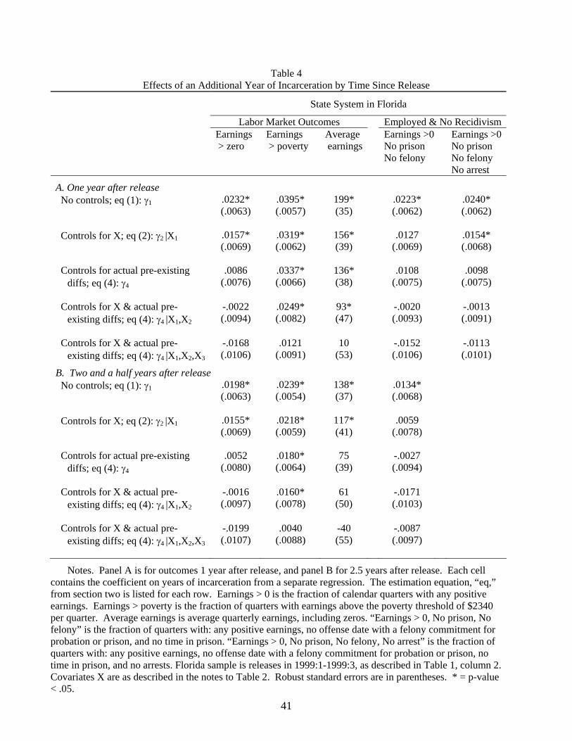
41
Table 4 Effects of an Additional Year of Incarceration by Time Since Release
State System in Florida
Labor Market Outcomes Employed & No Recidivism Earnings
> zero Earnings > poverty
Average earnings
Earnings >0 No prison No felony
Earnings >0 No prison No felony No arrest
A. One year after release
No controls; eq (1): γ1 .0232* (.0063)
.0395* (.0057)
199* (35)
.0223* (.0062)
.0240* (.0062)
Controls for X; eq (2): γ2 |X1 .0157*
(.0069) .0319* (.0062)
156* (39)
.0127 (.0069)
.0154* (.0068)
Controls for actual pre-existing
diffs; eq (4): γ4 .0086
(.0076) .0337* (.0066)
136* (38)
.0108 (.0075)
.0098 (.0075)
Controls for X & actual pre-
existing diffs; eq (4): γ4 |X1,X2 -.0022 (.0094)
.0249* (.0082)
93* (47)
-.0020 (.0093)
-.0013 (.0091)
Controls for X & actual pre-
existing diffs; eq (4): γ4 |X1,X2,X3 -.0168 (.0106)
.0121 (.0091)
10 (53)
-.0152 (.0106)
-.0113 (.0101)
B. Two and a half years after release
No controls; eq (1): γ1 .0198* (.0063)
.0239* (.0054)
138* (37)
.0134* (.0068)
Controls for X; eq (2): γ2 |X1 .0155*
(.0069) .0218* (.0059)
117* (41)
.0059 (.0078)
Controls for actual pre-existing
diffs; eq (4): γ4 .0052
(.0080) .0180* (.0064)
75 (39)
-.0027 (.0094)
Controls for X & actual pre-
existing diffs; eq (4): γ4 |X1,X2 -.0016 (.0097)
.0160* (.0078)
61 (50)
-.0171 (.0103)
Controls for X & actual pre-
existing diffs; eq (4): γ4 |X1,X2,X3 -.0199 (.0107)
.0040 (.0088)
-40 (55)
-.0087 (.0097)
Notes. Panel A is for outcomes 1 year after release, and panel B for 2.5 years after release. Each cell contains the coefficient on years of incarceration from a separate regression. The estimation equation, “eq,” from section two is listed for each row. Earnings > 0 is the fraction of calendar quarters with any positive earnings. Earnings > poverty is the fraction of quarters with earnings above the poverty threshold of $2340 per quarter. Average earnings is average quarterly earnings, including zeros. “Earnings > 0, No prison, No felony” is the fraction of quarters with: any positive earnings, no offense date with a felony commitment for probation or prison, and no time in prison. “Earnings > 0, No prison, No felony, No arrest” is the fraction of quarters with: any positive earnings, no offense date with a felony commitment for probation or prison, no time in prison, and no arrests. Florida sample is releases in 1999:1-1999:3, as described in Table 1, column 2. Covariates X are as described in the notes to Table 2. Robust standard errors are in parentheses. * = p-value < .05.

42
Table 5 Subgroup Effects of an Additional Year of Incarceration
on Labor Market Outcomes Seven Years After Incarceration Began
State System in Florida Controls for X and actual pre-existing diffs; eq (4): γ4 |X1,X2,X3 Earnings > zero Earnings > poverty Average earnings
A. Education Not high school graduate n=4971
.0112 (.0090)
.0029 (.0070)
27 (46)
High school graduate or some college n=1850
-.0035 (.0150)
-.0076 (.0123)
-94 (92)
Difference n=6821
.0147 (.0174)
.0105 (.0141)
122 (101)
B. Self-reported employment
Not employed at arrest n=2416
-.0117 (.0120)
-.0189* (.0087)
-116* (57)
Employed at arrest n=4405
.0205 (.0107)
.0129 (.0083)
77 (59)
Difference n=6821
-.0322 (.0168)
-.0318* (.0125)
-193* (84)
C. Race
Non-white n=3963
.0173 (.0097)
.0098 (.0072)
49 (47)
White n=2858
-.0029 (.0125)
-.0092 (.0099)
-49 (73)
Difference n=6821
.0202 (.0159)
.0190 (.0125)
98 (86)
D. Prior incarceration
Prior incarceration n=3306
.0100 (.0109)
.0048 (.0078)
15 (53)
No prior incarceration n=3515
.0084 (.0116)
-.0016 (.0092)
-7 (62)
Difference n=6821
.0016 (.0167)
.0064 (.0123)
22 (80)
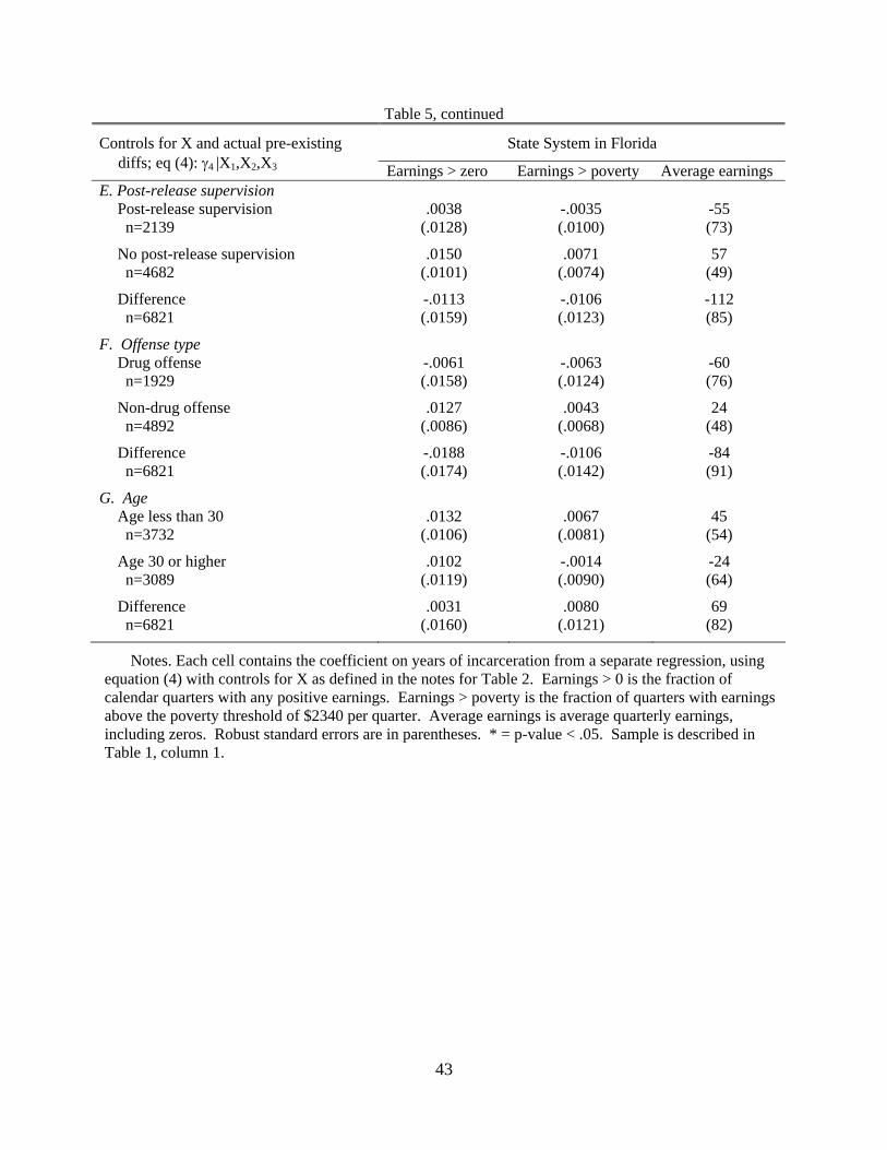
43
Table 5, continued
State System in Florida Controls for X and actual pre-existing diffs; eq (4): γ4 |X1,X2,X3 Earnings > zero Earnings > poverty Average earnings
E. Post-release supervision Post-release supervision n=2139
.0038 (.0128)
-.0035 (.0100)
-55 (73)
No post-release supervision n=4682
.0150 (.0101)
.0071 (.0074)
57 (49)
Difference n=6821
-.0113 (.0159)
-.0106 (.0123)
-112 (85)
F. Offense type
Drug offense n=1929
-.0061 (.0158)
-.0063 (.0124)
-60 (76)
Non-drug offense n=4892
.0127 (.0086)
.0043 (.0068)
24 (48)
Difference n=6821
-.0188 (.0174)
-.0106 (.0142)
-84 (91)
G. Age
Age less than 30 n=3732
.0132 (.0106)
.0067 (.0081)
45 (54)
Age 30 or higher n=3089
.0102 (.0119)
-.0014 (.0090)
-24 (64)
Difference n=6821
.0031 (.0160)
.0080 (.0121)
69 (82)
Notes. Each cell contains the coefficient on years of incarceration from a separate regression, using equation (4) with controls for X as defined in the notes for Table 2. Earnings > 0 is the fraction of calendar quarters with any positive earnings. Earnings > poverty is the fraction of quarters with earnings above the poverty threshold of $2340 per quarter. Average earnings is average quarterly earnings, including zeros. Robust standard errors are in parentheses. * = p-value < .05. Sample is described in Table 1, column 1.

44
Appendix Table A1 Regression Coefficients Explaining Quarterly Wages Seven Years After Incarceration
For the State System in Florida, Controlling for Subsets of X1 Incarceration length 6
(32) -18 (33)
23 (33)
9 (34)
Offense Murder/manslaughter
801 (345)
628 (339)
Offense Sexual behavior
552 (176)
366 (176)
Offense Robbery
9 (126)
-59 (125)
Offense Other violent
152 (127)
99 (126)
Offense Burglary
-147 (113)
-158 (111)
Offense Property theft/fraud
130 (123)
67 (122)
Offense Drug trafficking
47 (122)
58 (123)
Offense Weapons
275 (209)
295 (211)
Offense Other
88 (185)
42 (180)
Female 8
(102) 0
(103)
Black -74
(62) -77 (64)
Hispanic -107
(160) -99
(160)
Age 17
(31) 17
(31)
Age squared -0.28
(0.39) -0.31 (0.39)
Education <= 6 years -521
(212) -505 (212)
Education = 7 years -712
(127) -705 (128)
Education = 8 years -555
(113) -546 (113)
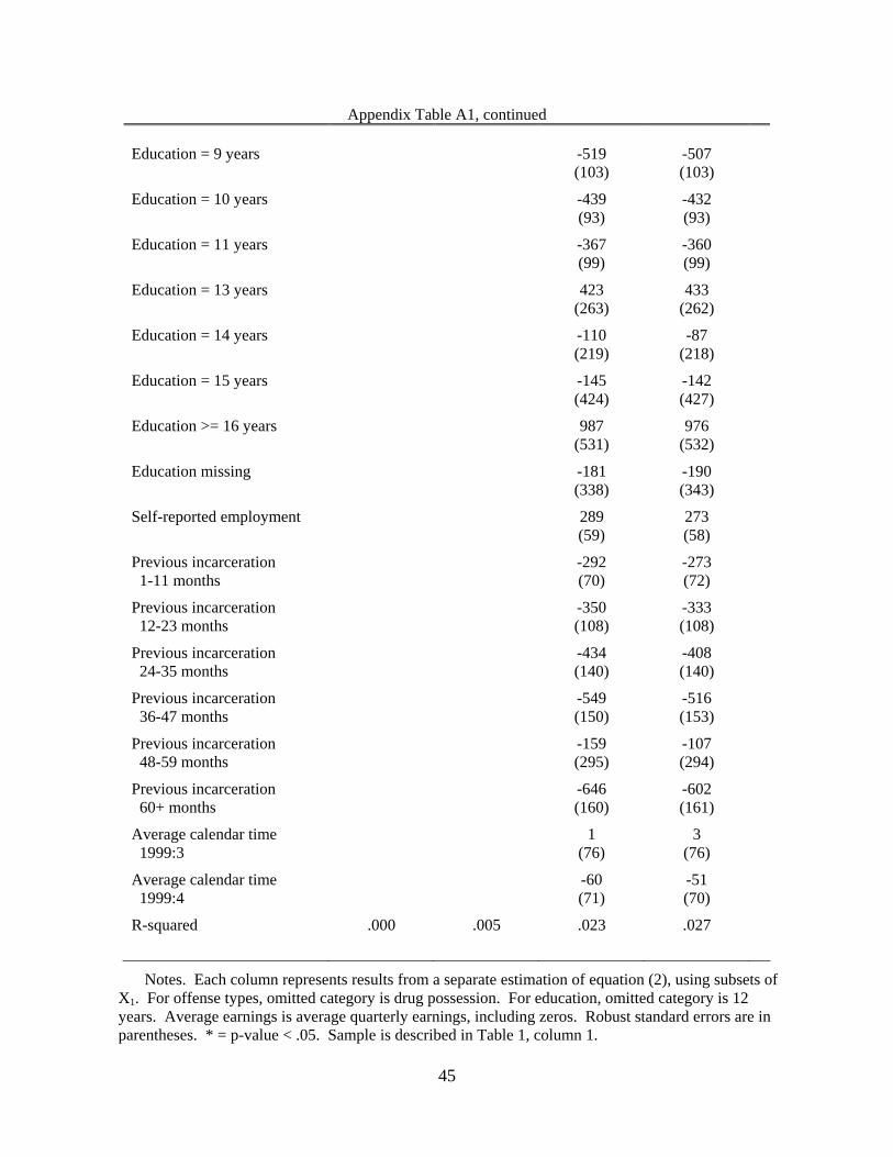
45
Appendix Table A1, continued Education = 9 years -519
(103) -507 (103)
Education = 10 years -439
(93) -432 (93)
Education = 11 years -367
(99) -360 (99)
Education = 13 years 423
(263) 433
(262)
Education = 14 years -110
(219) -87
(218)
Education = 15 years -145
(424) -142 (427)
Education >= 16 years 987
(531) 976
(532)
Education missing -181
(338) -190 (343)
Self-reported employment 289
(59) 273 (58)
Previous incarceration 1-11 months
-292 (70)
-273 (72)
Previous incarceration 12-23 months
-350 (108)
-333 (108)
Previous incarceration 24-35 months
-434 (140)
-408 (140)
Previous incarceration 36-47 months
-549 (150)
-516 (153)
Previous incarceration 48-59 months
-159 (295)
-107 (294)
Previous incarceration 60+ months
-646 (160)
-602 (161)
Average calendar time 1999:3
1 (76)
3 (76)
Average calendar time 1999:4
-60 (71)
-51 (70)
R-squared .000 .005 .023 .027
Notes. Each column represents results from a separate estimation of equation (2), using subsets of X1. For offense types, omitted category is drug possession. For education, omitted category is 12 years. Average earnings is average quarterly earnings, including zeros. Robust standard errors are in parentheses. * = p-value < .05. Sample is described in Table 1, column 1.

46
Appendix Table A2 Effects of Incarceration By Year of Spell Length
On Labor Market Outcomes Seven Years After Incarceration Began
State System in Florida
Earnings > zero Earnings > poverty Average earnings A. No controls; eq (1): γ1
2 Years Incarceration vs. 1 Year .0042 (.0145)
-.0082 (.0105)
-32 (74)
3 Years Incarceration vs. 1 Year -.0254
(.0184) -.0171 (.0138)
-96 (96)
4 Years Incarceration vs. 1 Year .0288
(.0249) .0056
(.0187) -3
(120) P-value for F-test that coefficients
for 2, 3, and 4 years are zero
.19
.58
.78 B. Controls for X and actual pre-existing
diffs; eq (4): γ4 |X1,X2,X3
2 Years Incarceration vs. 1 Year .0095 (.0151)
-.0066 (.0115)
-27 (77)
3 Years Incarceration vs. 1 Year -.0068
(.0202) -.0100 (.0152)
-62 (107)
4 Years Incarceration vs. 1 Year .0423
(.0270) .0085
(.0208) 32
(135) P-value for F-test that coefficients
for 2, 3, and 4 years are zero
.30
.80
.89
Notes. Each column in each panel contains results from a separate regression. Panel A uses equation (1) and panel B uses equation (4) with controls for X as defined in the notes for Table 2. Incarceration length is entered as a set of three indicators, with coefficients corresponding to the three rows in each panel and length of one year as the omitted category. Earnings > 0 is the fraction of calendar quarters with any positive earnings. Earnings > poverty is the fraction of quarters with earnings above the poverty threshold of $2340 per quarter. Average earnings is average quarterly earnings, including zeros. Robust standard errors are in parentheses. * = p-value < .05. Sample is described in Table 1, column 1.