inc341 frequency response method (continue)
DESCRIPTION
INC341 Frequency Response Method (continue). Lecture 12. Knowledge Before Studying Nyquist Criterion. unstable if there is any pole on RHP (right half plane). Open-loop system:. Characteristic equation:. poles of G(s)H(s) and 1+ G(s)H(s) are the same. Closed-loop system:. - PowerPoint PPT PresentationTRANSCRIPT

INC 341 PT & BP
INC341Frequency Response Method
(continue)
Lecture 12
INC 341 PT & BP
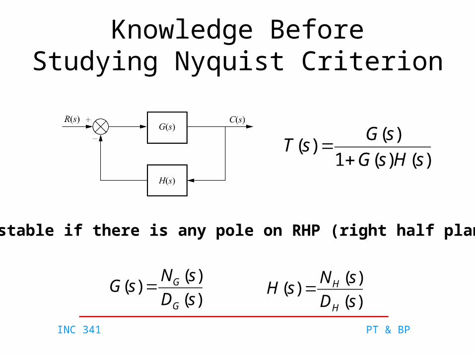
Knowledge BeforeStudying Nyquist Criterion
)()(1
)()(
sHsG
sGsT
)(
)()(
sD
sNsG
G
G)(
)()(
sD
sNsH
H
H
unstable if there is any pole on RHP (right half plane)

INC 341 PT & BP
)()()()(
)()(
)()(1
)()(
sNsNsDsD
sDsN
sHsG
sGsT
HGHG
HG
)(
)(
)(
)()()(
sD
sN
sD
sNsHsG
H
H
G
G
HG
HGHG
HG
HG
DD
NNDD
DD
NNsHsG
1)()(1
poles of G(s)H(s) and 1+G(s)H(s) are the same
zero of 1+G(s)H(s) is pole of T(s)
Characteristic equation:
Open-loop system:
Closed-loop system:
INC 341 PT & BP
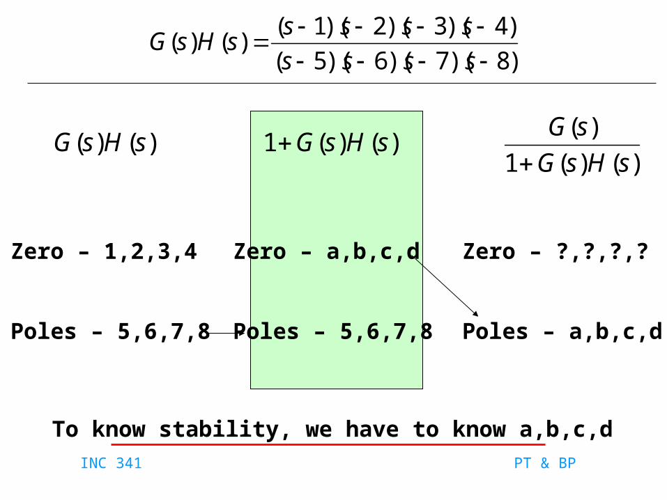
)8)(7)(6)(5(
)4)(3)(2)(1()()(
ssss
sssssHsG
)()(1
)(
sHsG
sG
)()( sHsG )()(1 sHsG
Zero – 1,2,3,4
Poles – 5,6,7,8
Zero – a,b,c,d
Poles – 5,6,7,8
Zero – ?,?,?,?
Poles – a,b,c,d
To know stability, we have to know a,b,c,d

INC 341 PT & BP
Stability from Nyquist plot
From a Nyquist plot, we can tell a number of closed-loop poles on the right half plane.– If there is any closed-loop pole on the right
half plane, the system goes unstable.– If there is no closed-loop pole on the right
half plane, the system is stable.

INC 341 PT & BP
Nyquist Criterion
Nyquist plot is a plot used to verify stabilityof the system.
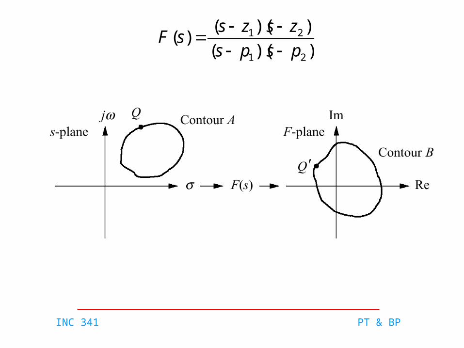
function))((
))(()(
21
21
psps
zszssF
mapping all points (contour) from one plane to anotherby function F(s).
mapping contour
INC 341 PT & BP
))((
))(()(
21
21
psps
zszssF
INC 341 PT & BP
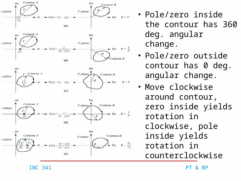
• Pole/zero inside the contour has 360 deg. angular change.
• Pole/zero outside contour has 0 deg. angular change.
• Move clockwise around contour, zero inside yields rotation in clockwise, pole inside yields rotation in counterclockwise

INC 341 PT & BP
Characteristic equation
N = P-ZN = # of counterclockwise direction about the origin
P = # of poles of characteristic equation inside contour
= # of poles of open-loop system
z = # of zeros of characteristic equation inside contour
= # of poles of closed-loop system
Z = P-N
)()(1)( sHsGsF
INC 341 PT & BP
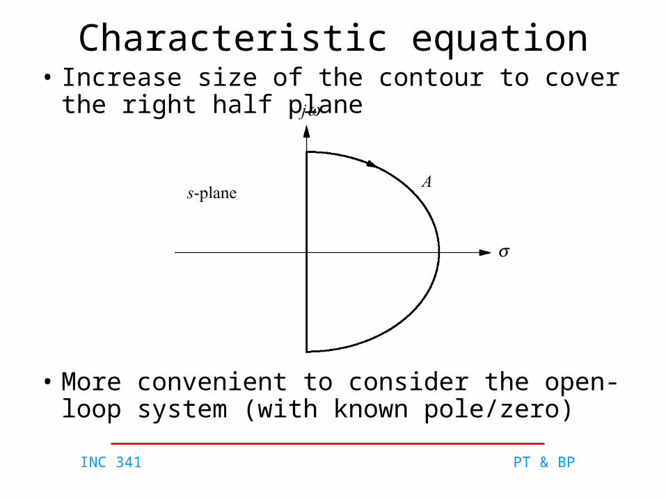
Characteristic equation• Increase size of the contour to cover the
right half plane
• More convenient to consider the open-loop system (with known pole/zero)

INC 341 PT & BP
‘Open-loop system’
Mapping from characteristic equ. to open-loop system by shifting to the left one step
Z = P-N
Z = # of closed-loop poles inside the right half plane
P = # of open-loop poles inside the right half plane
N = # of counterclockwise revolutions around -1
)()( sHsGNyquist diagram of

INC 341 PT & BP

INC 341 PT & BP
Properties of Nyquist plotIf there is a gain, K, in front of open-loop transfer function, the Nyquist plot will expand by a factor of K.

INC 341 PT & BP
Nyquist plot example
2
1)(
s
sG
• Open loop system has pole at 2
• Closed-loop system has pole at 1
• If we multiply the open-loop with a gain, K, then we can move the closed-loop pole’s position to the left-half plane
)1(
1
)(1
)(
sSG
sG

INC 341 PT & BP
Nyquist plot example (cont.)
• New look of open-loop system:
• Corresponding closed-loop system:
• Evaluate value of K for stability
2)(
s
KsG
)2()(1
)(
Ks
K
sG
sG
2K
INC 341 PT & BP
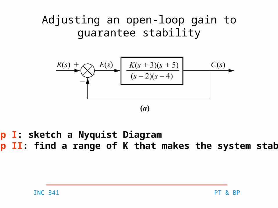
Adjusting an open-loop gain to guarantee stability
Step I: sketch a Nyquist DiagramStep II: find a range of K that makes the system stable!
INC 341 PT & BP
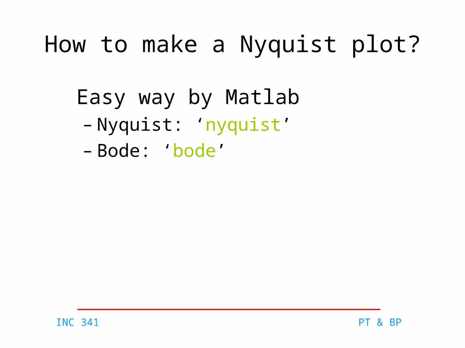
How to make a Nyquist plot?
Easy way by Matlab– Nyquist: ‘nyquist’– Bode: ‘bode’

INC 341 PT & BP
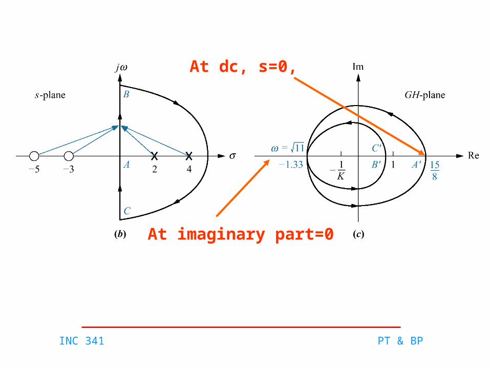
Step I: make a Nyquist plot
• Starts from an open-loop transfer function (set K=1)
• Set and find frequency response– At dc,– Find at which the imaginary part equals zero
js 00 s

INC 341 PT & BP
2222
3222
2
2
2
2
2
2
2
2
2
2
6)8(
)14154(48)8)(15(
6)8(
6)8(
6)8(
8)15(
6)8(
8)15(
86
158)()(
86
158
)4)(2(
)5)(3()()(
j
j
j
j
j
j
j
j
jjHjG
ss
ss
ss
sssHsG
11,0Need the imaginary term = 0,
31.1412
540
)11(6)118(
)11(48)118)(1115(22
Substitute back in to the transfer functionAnd get
1133.1)( sG
INC 341 PT & BP
At dc, s=0,
At imaginary part=0

INC 341 PT & BP
Step II: satisfying stability condition
• P = 2, N has to be 2 to guarantee stability• Marginally stable if the plot intersects -1• For stability, 1.33K has to be greater than 1
K > 1/1.33
or K > 0.75

INC 341 PT & BP
ExampleEvaluate a range of K that makes the system stable
)2)(22()(
2
sss
KsG

INC 341 PT & BP
22222
22
2
)6()1(16
)6()1(4
)2)(22)(()(
j
jjj
KjG
At 6,0 the imaginary part = 0
Plug back in the transfer functionand get G = -0.05
Step I: find frequency at which imaginary part = 0
js Set
6

INC 341 PT & BP
Step II: consider stability condition
• P = 0, N has to be 0 to guarantee stability• Marginally stable if the plot intersects -1• For stability, 0.05K has to be less than 1
K < 1/0.05
or K < 20

INC 341 PT & BP
Gain Margin and Phase Margin
Gain margin is the change in open-loop gain (in dB),required at 180 of phase shift to make the closed-loopsystem unstable.
Phase margin is the change in open-loop phase shift,required at unity gain to make the closed-loopsystem unstable.
GM/PM tells how much system can toleratebefore going unstable!!!

INC 341 PT & BP
GM and PM via Nyquist plot

INC 341 PT & BP
GM and PM via Bode Plot
MG
M
•The frequency at which the phase equals 180 degrees is called the phase crossover frequency
•The frequency at which the magnitude equals 1 is called the gain crossover frequency
MG
gain crossover frequency phase crossover frequency

INC 341 PT & BP
Example
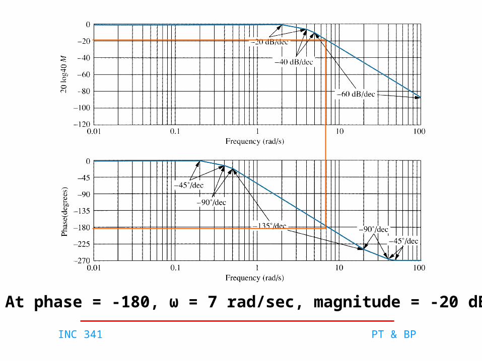
Find Bode Plot and evaluate a value of Kthat makes the system stableThe system has a unity feedback with an open-loop transfer function
)5)(4)(2()(
sss
KsG
First, let’s find Bode Plot of G(s) by assuming that K=40 (the value at which magnitude plotstarts from 0 dB)
INC 341 PT & BP
At phase = -180, ω = 7 rad/sec, magnitude = -20 dB

INC 341 PT & BP
• GM>0, system is stable!!!
• Can increase gain up 20 dB without causing instability (20dB = 10)
• Start from K = 40
• with K < 400, system is stable

INC 341 PT & BP
Closed-loop transient and closed-loop frequency responses
‘2nd system’
22
2
2)(
)(
)(
nn
n
sssT
sR
sC

INC 341 PT & BP
Magnitude Plot of closed-loop system
Damping ratio and closed-loop frequency response
212
1
pM
221 np

INC 341 PT & BP
244)21(1
244)21(4
244)21(
242
2
242
242
p
BW
sBW
nBW
T
T
= frequency at which magnitude is 3dB down
from value at dc (0 rad/sec), or .
Response speed and closed-loop frequency response
BW
2
1M

INC 341 PT & BP
Find from Open-loop Frequency Response
BW
Nichols Charts
From open-loop frequency response, we can find at the open-loop frequency that the magnitudelies between -6dB to -7.5dB (phase between -135 to -225) BW

INC 341 PT & BP
Relationship betweendamping ratio and phase marginof open-loop frequency response
42
1
412
2tan
M
Phase margin of open-loop frequency responseCan be written in terms of damping ratio as following
INC 341 PT & BP
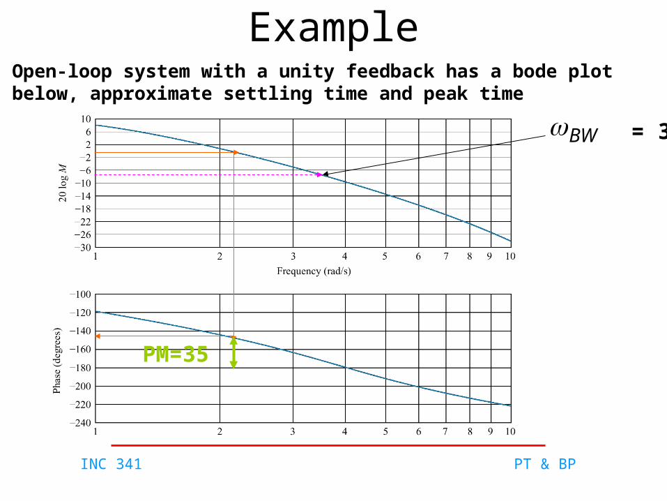
ExampleOpen-loop system with a unity feedback has a bode plot below, approximate settling time and peak time
= 3.7BW
PM=35

INC 341 PT & BP
32.0
412
2tan
42
1
M
Solve for PM = 35
43.1
244)21(1
5.5
244)21(4
242
2
242
BW
p
BWs
T
T