Introduction

In this chapter we will mainly disscuss second order linear di�erential equations of form

y00 + p(t)y0 + q(t) = g(t)

for all t 2 I. Here I is some open interval, whereas p(t), q(t) and g(t) are assumed continuous on

the whole interval I.

De�nition: A second order linear di�erential equation is said to be homogeneous if g(t) � 0, for

all t 2 I. Otherwise, the equation is said to be non-homogeneous.

We shall begin with the following theorem of (global) existence and uniqueness.

Theorem: If p(t), q(t), and g(t) are continuous on some open interval I, then there exists a unique

solution, throughout whole interval I, to the following initial value problem

y00 + p(t)y0 + q(t)y = g(t); y(t0) = y0; y

0(t0) = y00:

Here t0 2 I, y0 and y00 are two arbitrary constants.

A proof of the proof is presented in the next section.

However, here we want to point out that a second order linear equation can be transformed

into a two-dimensional system of �rst order linear di�erential equations. Actually, let us di�ne

z1(t)4= y(t); z2(t)

4= y

0(t):

The initial value problem can be written as the following two-dimensional linear system

z01 = z2

z02 = �q(t)z1 � p(t)z2 + g(t)

with initial condition

z1(t0) = y0; z2(t0) = y00:

We can write this in a more compact way using matrix. De�ne

Z(t)4=

�z1(t)

z2(t)

�=

�y(t)

y0(t)

�; A(t)

4=

�0 1

�p(t) �q(t)

�; B(t)

4=

�0

g(t)

�; Z0

4=

�y0

y00

�:

We have a linear system of �rst order di�erential equations that looks much familiar.

Z0 = A(t) � Z +B(t); Z(t0) = Z0:

1

Remark: The above methodology works for linear di�erential equations of any order. That is,

linear di�erential equations of order n can be transformed into an n-dimensional system of

�rst order linear equations.

Remark: It is not diÆcult to see that nonlinear di�erential equations of any order can be trans-

formed into an n-dimensional (non-linear) system of �rst order di�erential equations.

Example: Change the following second-order equations to a �rst-order system.

y00 � 5y0 + ty = 3t2; y(0) = 0; y

0(0) = 1:

Solution: Let us de�ne

Z(t)4=

�z1(t)

z2(t)

�=

�y(t)

y0(t)

�:

We have

Z0 =

�0 1

5 �t

�� Z +

�0

3t2

�; Z(0) =

�0

1

�:

Example (Reverse): Consider the following system of �rst-order linear equations.

Z0 =

�3 2

1 �1

�� Z; here Z =

�z1

z2

�

Find the second-order linear di�erential equation that z1 satis�es.

Solution: The system is

z01 = 3z1 + 2z2

z02 = z1 � z2

It follows that

z01 + 2z02 = 5z1 ) w

0 = z1; where w4=z1 + 2z2

5

This implies that

w0 = z1

z01 = 3z1 + 2z2 = 3z1 + (5w � z1) = 5w + 2z1:

Therefore, we have

z001 = 5w0 + 2z01 = 5z1 + 2z01 ) z

001 � 2z01 � 5z1 = 0:

Example: Consider the following system of �rst order linear equations.

z01 = z1 + z2

z02 = z1 � 2z2

Write out the di�erential equation z1 satis�es.

2

Solution: To obtain the equation of z1, we have

2z01 + z02 = 3z1 ) z1 =

�2z1 + z2

3

�0:= w

0 where w =2z1 + z2

3:

It follows that

z01 = z1 + z2 = z1 + 3w � 2z1 = 3w � z1

which implies that

z001 = 3w0 � z

01 = 3z1 � z

01 or z

001 + z

01 � 3z1 = 0

Exercise: Redo the preceding example for z2.

Solution: We have

z01 � z

02 = 3z2 ) z2 =

�z1 � z2

3

�0:= w

0 where w =z1 � z2

3:

It follows that

z02 = z1 � 2z2 = 3w + z2 � 2z2 = 3w � z2

which implies that

z002 = 3w0 � z

02 = 3z2 � z

02 or z

002 + z

02 � 3z2 = 0

Remark: Note that the equations for z1 and z2 are the same. It is actually a general phenomenon.

Exercise: Change the following third-order linear di�erential equation into a 3-dimensional system

of �rst-order linear equations.

y000 � e

ty0 + 2y = e

2t

Solution: Let z14= y, z2

4= y

0, and z34= y

00. We have

z01 = z2

z02 = z3

z03 = �2z1 + e

tz2 + e

2t

or

Z0 =

24 0 1 0

0 0 1

�2 et 0

35 � Z +

24 0

0

e2t

35

3

1 Proof of Theorem

To prove the existence and uniqueness, we shall use again the method of successive approximation.

Consider the equilavent two-dimenasional linear system of �rst order di�erential equations

Z0 = A(t) � Z +B(t); Z(t0) = Z0;

as constructed in Introduction. It is not very diÆcult to see that there exists a positive number K

such that

kA(t)Zk � KkZk

for all t 2 [a; b] and Z 2 IR2. Here kZk 4=pz21 + z22 . Let

�0(t) � Z0 =

�y0

y00

�and succesively, we de�ne

�n+1(t) = Z0 +

Z t

t0

�A(s) � �n(s) +B(s)

�ds

It follows that

k�n+1(t)� �n(t)k �Z t

t0

kA(s) ���n(s)� �n�1(s)

�k dt � K

Z t

t0

k�n(s)� �n�1(s)k ds:

However, we have

k�1(t)� �0(t)k �Z t

t0

kA(s) � Z0 +B(s)k ds �M(t� t0);

here

M4= KkZ0k+ max

s2[a;b]kB(s)k:

An easy induction yields that

k�n+1(t)� �n(t)k �MKn (t� t0)

n

(n+ 1)!�MK

n (b� a)n

(n+ 1)!

Since 1Xn=1

MKn (b� a)n

(n+ 1)!<1;

iterative sequence f�n(t);n = 0; 1; 2; � � � g converges uniformly to some function �(t). It follows that

�(t) is our solution.

The uniqueness follows from the Gronwall Inequality. Suppose that �(t) and '(t) are two

solutions to the equation, it follows that

k�(t)� '(t)k �Z t

t0

Kk�(s)� '(s)k ds

Letting v(t)4= k�(t)� '(t)k, we have

v(t) �Z t

t0

Kv(s) ds; v(t0) = 0

Hence v(t) � 0 by Gronwall inequality. This completes the proof. 2

4

2 Linear Independence; Fundamental Solutions

The theorem of existence and uniqueness provides an excellent way to obtain all solutions to second

order linear di�erential equations. In this section we exclusively consider homogeneous case, that

is, g(t) � 0. Our equation, therefore, is

y00 + p(t)y0 + q(t)y = 0:

An immediate result is the so-called Principle of Superposition.

Proposition (Principle of Superposition): If y1 and y2 are two solutions of the homogeneous

di�erential equation

y00 + p(t)y0 + q(t)y = 0;

then any linear combination of y1 and y2, say c1y1 + c2y2, is also a solution. Here c1 and c2

are arbitrary contants.

Proof: Use formulae (�1 + �2)0 = �

01 + �

02, (c�)

0 = c�0. 2

Before we present the main theorem, let us read several examples to see how it works.

Example: Solve the following initial value problem

y00 � 3y0 + 2y = 0; y(0) = 1; y

0(0) = 1

Solution: We guess a solution to the di�erential equation

y00 � 3y0 + 2y = 0

will take form y(t) = ert. It follows that�ert�00 � 3

�ert�0+ 2ert = e

rt � (r2 � 3r + 2) = 0

If we choose r as a root of the following algebric equation (characteristic equation)

r2 � 3r + 2 = 0 ) r1 = 1; r2 = 2;

then y = ert will solve the di�erential equation. Moreover, any linear combination of er1t and

er2t will also solve the di�erential equation.

Now we guess that the solution to the initial value problem will take form

y(t) = c1er1t + c2e

r2t:

This function y(t) will satisfy y00 � 3y0 + 2y = 0 regardless of what values c1 and c2 take.

The remaining question is whether we can �nd a suitable pair (c1; c2) such that the initial

conditions are satis�ed. But this is equivalent to the following equation

y(0) = c1 + c2 = 1; y0(0) = c1r1 + c2r2 = c1 + 2c2 = 1

This implies c1 = 1; c2 = 0. Hence y(t) = et is a solution to the initial value problem.

Furthermore, it follows from previous theorem that it is actually the only solution to the

initial value problem.

5

Exercise: In the above initial value problem, if we change the initial conditions to the more general

y(0) = y0, y0(0) = y

00, can we still �nd the unique solution?

Solution: The only di�erence would be that (c1; c2) shall satisfy

c1 + c2 = y0; c1 + 2c2 = y00:

For any values of y0 and y00, the above linear equation system is solvable with solution

c1 = 2y0 � y00; c2 = y

00 � y0:

The solution to the initial value problem is

y(t) = (2y0 � y00)e

t + (y00 � y0)e2t

We can conclude from the example one way to solve a general second-order linear second-order

di�erential equation.

Step 1a. Find two solutions, say y1(t) and y2(t), of di�erential equation

y00 + p(t)y + q(t) = 0:

Step 1b. The two solutions, y1(t) and y2(t), shall have the following property: for any initial

condition y(t0) = y0, y0(t0) = y

00, we can �nd constants (c1; c2) such that

y(t)4= c1y1(t) + c2y2(t)

satis�es the initial condition.

Step 2. By the principle of superposition, we know y(t) is a solution of the initial value problem.

By the theorem of existence and uniqueness, we know y(t) is actually the unique solution to

the initial value problem.

It is not diÆcult to see that step 1b is equivalent to solving the following linear equations

y0 = c1y1(t0) + c2y2(t0)

y00 = c1y

01(t0) + c2y

02(t0)

However, this system of equations would be solvable for all y0 and y00 if and only if the determinant

det

�y1(t0) y2(t0)

y01(t0) y

02(t0)

�= y1(t0)y

02(t0)� y

01(t0)y2(t0) 6= 0:

The determinant is called Wronskian determinant, or simply Wronskian, of the solutions y1; y2. It

will be denoted by W (y1; y2)(t0), or simply W (t0) when no confusion is incurred.

Example(continued): In the previous example, the Wronskian is

W (t) = y1(t)y02(t)� y

01(t)y2(t) = e

t � 2e2t � et � e2t = e

3t 6= 0:

6

It follows from above discussion that step 1a+1b is equivalent to

Step 1: Find two solutions, say y1(t) and y2(t), whose Wronskian is non-zero. This shall allow us

to determine (c1; c2) for any initial condition.

Exercise: Show that

1. W (y; y) = 0

2. W (y1; y2) = �W (y2; y1)

3. W (y1 + y2; y) =W (y1; y) +W (y2; y)

4. W (ay1; y2) = aW (y1; y2)

for any di�erentiable function y1; y2; y and constant a.

Exercise: Show that for any constants a; b; c; d, any functions f; g, we have

W (af + bg; cf + dg) = (ad� bc)W (f; g):

Proof: We have

W (af + bg; cf + dg) = aW (f; cf + dg) + bW (g; cf + dg)

= a�cW (f; f) + dW (f; g)

�+ b�cW (g; f) + dW (g; g)

�= adW (f; g) + bcW (g; f) = (ad� bc)W (f; g)

E.g. W (2f + g; 3f � 2g) = (2 � (�2)� 1 � 3)W (f; g) = �7 �W (f; g).

2.1 Fundamental Solutions

The following two theorems will give an aÆrmative answer to the existence of such a pair of

solutions, and characterize all solutions to a given linear di�erential equation.

Theorem: Consider di�erential equation

y00 + p(t)y0 + q(t)y = 0;

where p, q are continuous functions on open interval I. There exist a pair of solutions y1 and

y2 such that every solution of the above di�erential equation, say �, can be represented as

the linear combination of y1 and y2. That is, for every solution �, there exist constants c1and c2 such that

� = c1y1 + c2y2:

Remark: Such a pair of solution (y1; y2) is called a fundamental set of solutions, while the expres-

sion y = c1y1 + c2y2 with arbitary coeÆcients (c1; c2) are called general solutions.

Theorem: Let y1; y2 be any two solutions to the di�erential equation. The following statements

are equivalent.

1. A pair of solution (y1; y2) is a fundamental set of solution.

7

2. The Wronskian W (t)4=W (y1; y2)(t) is not zero for all t 2 I.

3. The Wronskian W (t)4=W (y1; y2)(t) is not zero for some t0 2 I.

Proof of the �rst theorem: Fix any t0 2 I. Let y1 be the solution of the di�erential equation

with initial condition y1(t0) = 1, y01(t0) = 0. Similarly, let y2 be the solution with initail

condition y2(t0) = 0, y02(t0) = 1. Note y1 and y2 always exist. Now, let � be an arbitary

solution of di�erential equation. De�ne a4= �(t0), b

4= �

0(t0). Consider the following initial

value problem

y00 + p(t)y0 + q(t)y = 0; y(t0) = a; y

0(t0) = b:

We know � is a solution to this initial value problem. However, note that

~�4= ay1 + by2

is also a solution to the initial value problem (check!!). By uniqueness, we know

� = ~� = ay1 + by2:

This completes the proof. 2

Proof of the second theorem: We shall prove \2) 3) 1) 2". But \2) 3" is trivial.

\3) 1". The proof is very similar to that of the �rst theorem. The only di�erence is

~�4= Ay1 +By2

with A and B determined by equations

Ay1(t0) +By2(t0) = a

Ay01(t0) +By

02(t0) = b

Note such (A;B) always exist since W (t0) 6= 0 (check!!).

\1 ) 2". Fix an arbitrary s 2 I, let � be the solution to the di�erential equation with

initial condition �(s) = 1, �0(s) = 0. By de�nition, there exist constants (c1; c2) such that

� = c1y1 + c2y2. In particular

1 = c1y1(s) + c2y2(s); 0 = c1y01(s) + c2y

02(s)

Similarly, let ~� be the solution with initial condition ~�(s) = 0, ~�(s) = 1. There exist constants

(~c1; ~c2) such that ~� = ~c1y1 + ~c2y2. In particular

0 = ~c1y1(s) + ~c2y2(s); 1 = ~c1y01(s) + ~c2y

02(s):

However, this implies that,

[c1y1(s) + c2y2(s)]��~c1y

01(s) + ~c2y

02(s)

���c1y

01(s) + c2y

02(s)

��[~c1y1(s) + ~c2y2(s)] = 1�1�0�0 = 1

But the left hand side, by direct calculation, is

W (s) � (c1~c2 � ~c1c2) = 1 ) W (s) 6= 0

Since s is arbitrary, it completes the proof. 2

8

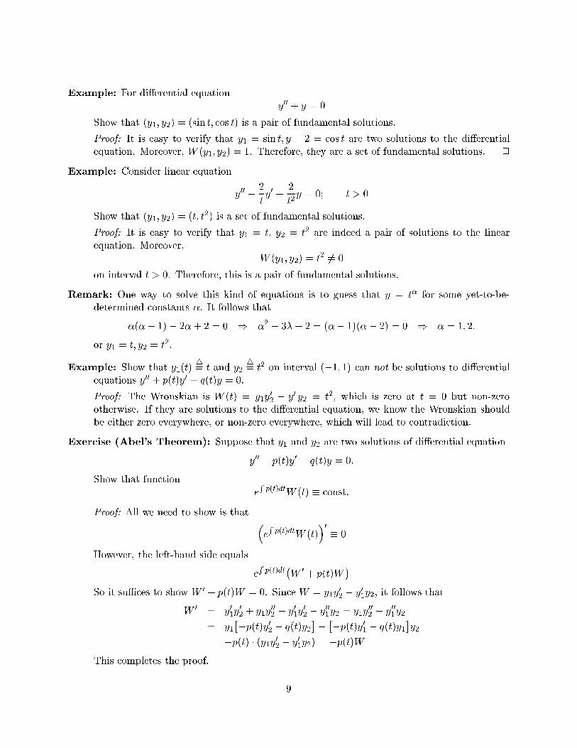
Example: For di�erential equation

y00 + y = 0

Show that (y1; y2) = (sin t; cos t) is a pair of fundamental solutions.

Proof: It is easy to verify that y1 = sin t; y � 2 = cos t are two solutions to the di�erential

equation. Moreover, W (y1; y2) = 1. Therefore, they are a set of fundamental solutions. 2

Example: Consider linear equation

y00 � 2

ty0 +

2

t2y = 0; t > 0

Show that (y1; y2) = (t; t2) is a set of fundamental solutions.

Proof: It is easy to verify that y1 = t, y2 = t2 are indeed a pair of solutions to the linear

equation. Moreover,

W (y1; y2) = t2 6= 0

on interval t > 0. Therefore, this is a pair of fundamental solutions.

Remark: One way to solve this kind of equations is to guess that y = t� for some yet-to-be-

determined constants �. It follows that

�(�� 1)� 2�+ 2 = 0 ) �2 � 3�+ 2 = (�� 1)(� � 2) = 0 ) � = 1; 2:

or y1 = t; y2 = t2.

Example: Show that y1(t)4= t and y2

4= t

2 on interval (�1; 1) can not be solutions to di�erential

equations y00 + p(t)y0 + q(t)y = 0.

Proof: The Wronskian is W (t) = y1y02 � y

01y2 = t

2, which is zero at t = 0 but non-zero

otherwise. If they are solutions to the di�erential equation, we know the Wronskian should

be either zero everywhere, or non-zero everywhere, which will lead to contradiction.

Exercise (Abel's Theorem): Suppose that y1 and y2 are two solutions of di�erential equation

y00 + p(t)y0 + q(t)y = 0:

Show that function

e

Rp(t)dt

W (t) � const.

Proof: All we need to show is that �e

Rp(t)dt

W (t)�0� 0

However, the left-hand side equals

e

Rp(t)dt

�W0 + p(t)W

�So it suÆces to show W

0 + p(t)W = 0. Since W = y1y02 � y

01y2, it follows that

W0 = y

01y02 + y1y

002 � y

01y02 � y

001y2 = y1y

002 � y

001y2

= y1

��p(t)y02 � q(t)y2

����p(t)y01 � q(t)y1

�y2

= �p(t) � (y1y02 � y01y2) = �p(t)W

This completes the proof.

9

Remark: This actually provide another way to show the equivalence of statement 2 and statement

3 in the second theorem.

One thing shall keep in mind though, fundamental set of solutions is not unique.

Example (Non-uniqueness of fundamental set of solutions): Suppose (y1; y2) is a funda-

mental set of solution to equation y00 + p(t)y0 + q(t)y = 0. Show that (y1 + cy2; y2) is also a

fundamental set of solutions, where c is an arbitrary constant.

2.2 Linear Independence

We can do an extension of the second theorem by introducing a new concept of linear independence.

De�nition: Two function f and g are said to be linearly dependent on interval I if there exist two

constants k1 and k2, not both zero, such that

k1f(t) + k2g(t) � 0

for all t 2 I. Otherwise, they are said to be linearly independent.

Example: Functions et and e�t are linearly independent on any interval, while sin t and sin(t+�)

are linearly dependent on any interval.

Example: Functions jtj and t are linear dependent on interval [0; 1), and linear dependent on

interval (�1; 0]. However, they are linear independent on interval (�1; 1).

Lemma: Suppose f and g are linear dependent on interval I, then W (f; g)(t) � 0 for every t 2 I.

Proof: Let k1 and k2 be two constants, not both zero, such that

k1f + k2g � 0 ) k1f0 + k2g

0 � 0

Without loss of generality, we assume k1 6= 0. We have

0 � (k1f + k2g)g0 � (k1f

0 + k1g0)g = k1W ) W � 0

This completes the proof. 2

Remark: The reverse of the lemma might not always hold true generally. For example, functions

f(t)4= tjtj and g(t)

4= t

2 are linear independent on interval (�1; 1). It is not diÆcult to show

that W (f; g)(t) � 0. Actually f 0(t) = 2jtj, g0(t) = 2t and

W (f; g) = tjtj � 2t� 2jtj � t2 = 0

Remark: The reverse of the lemma holds true in case both f and g are solutions to same di�erential

equation, as we shall see in next lemma.

10

Lemma: Suppose y1 and y2 are two solutions to di�erential equations

y00 + p(t)y0 + q(t)y = 0

on interval I, here p and q are continuous. Then y1 and y2 are linear dependent if and only

if W (y1; y2) � 0.

Proof: We only need to prove the suÆciency (Necessity is proved in the preceding lemma).

Fix any t0 2 I. From assumption, W (t0) = 0. Therefore, there exist two constants c1 and c2,

not both zero, such that

c1y1(t0) + c2y2(t0) = 0

c1y01(t0) + c2y2(t0) = 0

Let �4= c1y1 + c2y2. It follows that � is a solution to the initial value problem

y00 + p(t)y0 + q(t)y = 0; y(t0) = 0; y

0(t0) = 0

But constant 0 is also a solution to the initial value problem. By uniqueness, we have

�(t) = c1y1(t) + c2y2(t) � 0; 8 t 2 I

or y1 and y2 are linearly dependent. 2

Remark: We have actually obtained another equilavent condition for fundamental solutions.

2.3 Conclusion

Let p(t); q(t) be contiouous functions on interval I.

Fundamental theorem: There exists a unique solution to every initial value problem

y00 + p(t)y0 + q(t)y = 0; t 2 I; y(t0) = y0; y

0(t0) = y00

fundamental set of solutions: There exist a pair of solutions (y1; y2) to di�erential equation

y00 + p(t)y0 + q(t)y = 0; t 2 I;

such that any other solutions to this di�erential equation can be represented as a linear

combination of (y1; y2). In another word, the set

fc1y1 + c2y2; c1; c2 are arbitrary constantsg:

is the complete set of solutions to the di�erential equation. We call y = c1y1 + c2y2 general

solutions where c1; c2 are arbitrary constants.

Equivalence conditions for fundamental set of solutions: Consider a linear homogeneous equa-

tion

y00 + p(t)y0 + q(t)y = 0; t 2 I:

Suppose (y1; y2) is a pair of solutions to this di�erential equation. Then the following state-

ments are equilavent

11

1. (y1; y2) is a fundamental set of solutions.

2. The Wronskian of of (y1; y2), denoted by W (t), is non-zero for all t 2 I.

3. The Wronskian of of (y1; y2), denoted by W (t), is non-zero for some t0 2 I.

4. (y1; y2) are linear independent.

Corollary: Let (y1; y2) be a pair of solutions to di�erential equation

y00 + p(t)y0 + q(t)y = 0; t 2 I:

Then the Wrnoskian of (y1; y2) is either zero for all t 2 I, or non-zero for all t 2 I. Indeed,

we have the Abel Theorem:

W (y1; y2)(t) = ce�Rp(t) dt

for some constant c.

Corollary: Let (y1; y2) be a pair of solutions to di�erential equation

y00 + p(t)y0 + q(t)y = 0; t 2 I:

Then (y1; y2) are linear dependent on interval I if and only if the Wrnoskian of (y1; y2) are

zero for all t 2 I. Alternatively, (y1; y2) are linear independent on interval I if and only if the

Wrnoskian of (y1; y2) are non-zero for all t 2 I. (Note: the last claim is not true for a general

pair of functions).

The following examples illustrate the idea of solving a homogeneous equation of second order.

Example: Consider a di�erential equation

y00 + 3y0 + 2y = 0; t � 0

Guess a result of form y = ert, we have

(r2 + 3r + 2)ert � ) r2 + 3r + 2 = 0 ) r1 = �1; r2 = �2:

Therefore (e�t; e�2t) is a pair of solutions. However, their Wronskian is �e�3t in non-zero, so

this a fundamental set of solutions. The general solutions to this equations can be written as

y = c1e�t + c2e

�2t:

for arbitrary constants (c1; c2).

Now if we have initial conditions

y(0) = 0; y0(0) = 1;

we can solve a particular pair of (c1; c2) that

c1 + c2 = 0; � c1 � 2c� 2 = 1 ) c1 = 1; c2 = �1:

Or the solution to the initial value problem

y00 + 3y0 + 2y = 0; t � 0; y(0) = 0; y

0(0) = 1

is

�(t) = e�t � e

�2t:

12

3 Homogeneous Equations with Constant CoeÆcients

Second order linear di�erential equation with constant coeÆcients can be solved very easily, as we

shall see below. Consider equation

ay00 + by

0 + cy = 0

where a 6= 0, b and c are constants. From the discussion in previous section, it is suÆcient to obtain

a set of fundamental solutions. We seek a solution of form y = ert, where r is a parameter to be

determined. It follows that

ay00 + by

0 + cy = ert(ar2 + br + c) = 0:

This implies that r is the root of algebraic equation

ar2 + br + c = 0;

which is called characteristic equation. It follows that

r = r1;2 =�b�

pb2 � 4ac

2a

There are three possible scenarios, namely, the characteristic equation has two distinctive real

roots (b2�4ac > 0), two repeated real roots (b2�4ac = 0), two complex conjuate roots (b2�4ac < 0).

3.1 Two distinctive real roots (b2 � 4ac > 0)

If two real roots r1 6= r2, then y14= e

r1t and y24= e

r2t are both solutions to the di�erential equation.

Furthermore, their Wronskian is

W (t) = y1y02 � y

01y2 = e

r1t � r2er2t � r1er1t � er2t = (r2 � r1)e

(r1+r2)t 6= 0

It follows that y1 and y2 form a fundamental set of solutions. The general solution is therefore

y = c1y1 + c2y2 = c1er1t + c2e

r2t

Example: Solve the following initial value problem

y00 � 3y0 + 2y = 0; y(0) = 0; y0(0) = 1:

Solution: The characteristic equation is

r2 � 3r + 2 = 0 ) r1 = 1; r2 = 2:

Therefore the general solution is

y = c1et + c2e

2t:

Intial conditions implies

c1 + c2 = 0; c1 + 2c2 = 1 ) c1 = �1; c2 = 1

Therefore the solution to the initial value problem is

y = �et + e2t:

13

Example: A particle of mass m moving in a straight line is repelled from origin 0 by force F .

Assume the force is proportional to the distance of the particle from 0. Find the position of

the particle as a function of time if at t = 0, the particle has velocity 0 and it is l ft from the

origin.

Solution: Suppose at time t, the distance of the particle from origin is x(t). We have

md2x

dt2= F = kx:

The characteristic equation is

mr2 � k = 0 ) r1 =

rk

m; r2 = �

rk

m:

Therefore the general solution for the above di�erential equation is

x(t) = c1e

qkmt+ c2e

�q

kmt:

However, initial conditions x(0) = l, x0(0) = 0 imply that

c1 + c2 = l;

rk

m(c1 � c2) = 0 ) c1 = c2 =

l

2:

Or

x(t) =l

2

�e

qkmt+ e

�q

kmt

�:

Example (cont.): Suppose in the preceding example, the initial velocity of the particle is v (a

positive v means the velocity is away from origin, and a negative v means the velocity is

toward the origin). Find the critical value of v such that the particle will approach the origin

but never reach it.

Solution: Let x(t) be the distance of the particle from the origin at time t. It follows that

x(t) = c1e

qkmt+ c2e

�q

kmt

for some constants c1; c2. However, initial condition x(0) = l; x0(0) = v yields that

c1 + c2 = l;

rk

m(c1 � c2) = v ) c1 =

l + vp

mk

2; c2 =

l � vp

mk

2:

It follows that

x(t) =l + v

pmk

2e

qkmt+l � v

pmk

2e�q

kmt:

However,

limt!1

x(t) =

8>>><>>>:

+1 ; v > �lq

km

�1 ; v < �lq

km

0 ; v = �lq

km

9>>>=>>>;

Therefore, the critical velocity is �lq

km. 2

14

3.2 Two repeated real roots (b2 � 4ac = 0)

In case of b2 � 4ac = 0, we have r1 = r2 = �2ba:= r, and y1 = e

rt is a solution of the di�erential

equation. There are several ways to obtain a second solution { you can just guess-and-verify.

Lemma: If b2� 4ac = 0, then y2(t)4= te

rt is a solution of the di�erential equation. Here r = �2ba.

Proof: We have y02 = rtert + e

rt, y002 = r2te

rt + 2rert. Therefore

ay00 + by

0 + cy = (ar2 + br + c)tert + (2ra+ b)ert = 0

since 2ra+ b = 0 and ar2 + br + c = 0. 2

The Wroskian of y1 and y2 is

W (y1; y2)(t) = y1y02 � y

01y2 = e

rt � (rtert + ert)� re

rt � tert = e2rt 6= 0:

It follows that y1 and y2 are a fundamental set of solutions, and the general solution is

y = c1ert + c2te

rt:

Example: The general solution to di�erential equation

y00 + 4y0 + 4y = 0

is

y = c1e�2t + c2te

�2t:

Reduction of Order: This is another method of obtaining y2, Reduction of Order, which is of

some general interest. Actually, suppose we know a non-zero solution y1 to a general homo-

geneous linear di�erential equation

y00 + p(t)y + q(t)y = 0:

Assuming that y2(t) = v(t)y1(t) is a second solution, we have

y02 = v

0y1 + vy

01; y

002 = v

00y1 + 2v0y01 + vy

001

and

v00y1 + 2v0y01 + vy

001 + p(t)v0y1 + p(t)vy01 + q(t)vy = 0 ) y1v

00 +�2y01 + p(t)y1

�v0 = 0:

Letting w4= v

0, we obtain a �rst order di�erential equation

y1w0 +�2y01 + p(t)y1

�w = 0

This impliesw0

w= �2y01

y1� p(t) ) (ln jwj)0 = �

h2 ln jy1j+ e

Rp(t) dt

i0It follows that

w =c

e

Rp(t) dty

21

for some constant c 6= 0. It follows that v =Rw dt

15

Exercise: Prove that the Wronskian W (y1; y2)(t) 6= 0.

Proof: We have y02 = v0y1 + vy

01 = wy1 + vy

01. Hence

W (y1; y2) = y1y02 � y

01y2 = wy

21 = ce

�Rp(t) dt 6= 0:

This completes the proof. 2

Example: Find the general solution of

t2y00 � ty

0 + y = 0; t > 0

given that y1 = t is a solution.

Solution: By Reduction of Order method, assume y2(t) = v(t)y1(t) = tv(t). It follows that

t2(tv00 + 2v0)� t(tv0 + v) + tv = 0 ) t

3v00 + t

2v0 = 0 ) tv

00 + v0 = 0

Let w = v0, we have

tw0 + w = 0 ) w =

1

t; v = ln t:

Therefore y2 = t ln t is also solution. Therefore, the general solution is

y = c1t+ c2t log t:

Exercise: Use Reduction of Order to obtain y2 again in case of two repeated real roots.

3.3 Two conjuate complex roots (b2 � 4ac < 0)

If b2 � 4ac < 0, the characteristic equation admits two complex roots

r1;2 =�b�

pb2 � 4ac

2a= � b

2a�p4ac� b2

2ai := �� �i

Fromally, we have y1;2 = e(���i)t.

3.3.1 Review of Complex Analysis

For a complex number z = a + bi, a is called the real part, and b is called the imaginary part.

Here i is the imaginary unit with property i2 = �1. The conjuate of z, denoted by z, is de�ned as

z4= a� bi. The arithmetic rules of complex numbers are

(a1 + b1i) + (a2 + b2i) = (a1 + a2) + (b1 + b2)i

(a1 + b1i) � (a2 + b2i) = (a1a2 � b1b2) + (a1b2 + a2b1)i

Exercise: Show that

z1 + z2 = z1 + z2; z1 � z2 = z1 � z2

16

It will be convienent to represent a complex number on a plain geometrically; see the graph below.

Euler's Formula: We de�ne that

eit 4= cos t+ i sin t; 8 t 2 IR (Euler's Formula)

and

ez = e

a+bi 4= ea � ebi = e

a(cos b+ i sin b)

Example: ei�4 = cos �

4+ i sin �

4=

p22+ i

p22, e

i�2 = cos �

2+ i sin �

2= i, e

2+i = e2(cos 1+ i sin 1) =

7:39 � (0:54 + 0:84i) = 3:99 + 6:22i

Remark: (Motivation from Calculus) Taylor expansion yileds that

cos t = 1� t2

2!+t4

4!� t

6

6!+ � � �

sin t = t� t3

3!+t5

5!� t

7

7!+ � � �

We also have expansion

et = 1 +

t

1!+t2

2!+ � � � + t

n

n!+ � � �

If we are willing to replace t by it in the above expansion, we have

eit = 1 +

it

1!+

(it)2

2!+ � � �+ (it)n

n!+ � � �

=

�1� t

2

2!+t4

4!� t

6

6!+ � � �

�+

�t� t

3

3!+t5

5!� t

7

7!+ � � �

�i

= cos t+ i sin t

Exercise: 1. Show that eit1 � eit2 = ei(t1+t2), for all real numbers t1; t2. In general, ez1 � ez2 =

ez1+z2 , for allcomplex numbers z1; z2.

2. (de Moivre's Formula) Prove (cos' + i sin')n = cosn' + i sinn' (This provide a very

simple way to express cosn' and sinn' in terms of cos' and sin').

17

Derivative: The derivative of a complex function z(t) = f(t) + ig(t) is naturally de�ned as

dz

dt

4=df

dt+ i

dg

dt

Exercise: Show that ddtezt = ze

zt for any �xed complex number z.

Finally, we wish to point out that usual calculus rules also hold in complex analysis.

3.3.2 Real-Valued solutions

It follows that

y1;2 = e(���i)t = e

�t(cos�t � i sin�t)

are indeed two (complex) solutions of the di�erential equation (Exercise!). However, this implies

the linear combinations of y1 and y2,

u(t)4=y1 + y2

2= e

�t cos�t; v(t)4=y1 � y2

2i= e

�t sin�t

are also solutions to the di�erential equations.

Exercise: Use direct calculation to verify u and v are really solutions to the di�erential equation.

Exercise: Show that the Wronskian W (u; v) = �e2�t.

Since � =p4ac� b2 6= 0, the Wronskian W 6= 0, therefore u and v are a fundamental set of

solutions. The general solution of the di�erential solution is

y = c1e�t cos�t+ c2e

�t sin�t

Here are several examples.

Example: Find the general solution to the di�erential equation

y00 � 4y0 + 20y = 0; t � 0:

Show that any solution goes to 0 as t!1.

Solution: The characteristic equation is

r2 � 4r + 20 = 0 ) b

2 � 4ac = 16� 80 = �64 ) r1;2 =�4�

p�64

2= �2� 4i:

Therefore, the general solution is

y = c1e�2t cos 4t+ c2e

�2t sin 4t = e�2t(c1 cos 4t+ c2 sin 4t):

Since

jc1 cos 2t+ c2 sin 4tj � jc1j+ jc2jWe have y(t)! 0 as t!1. 2

18

Example: A displaced simple pendulum of length l, is attached with weight w = mg. Let �(t) be

the angle of swing at time t.

1. Find the di�erential equation � satis�es. Is this equation linear or nonlinear?

2. When the swing is very small, show that � satis�es a linear ODE approximately.

3. Find the period of this oscillation approximately.

Solution: The direction of the net external force must be in the direction tangent to the arc of

swing (there is should be no net force in the direction of the string). Therefore, the net force

is F = �mg sin � (the negative sign is because the direction of F is always in the opposition

direction of swing). We have, by Newton's law of force,

ma = �mg sin � where a is the acceleration:

However, if we let the s denote the distance the weight moves along the arc, we have s = l�,

hence

a =d2s

dt2= l

d2�

dt2

Therefore, the equation for � is

(*) ld2�

dt2+ g sin � = 0; or l�

00 + g sin � = 0

It is nonlinear. However, when the swing is small, we have sin � � � (why?), therefore, the

equation of � is approximately

ld2�

dt2+ g� = 0;

which is linear. For this equation, the characteristic equation is

lr2 + g = 0 ) r = �

rg

l

Therefore, the general solution is

� = c1 cos

rg

lt+ c2 sin

rg

lt:

The period is 2�q

lg. 2

19

Remark: Equation (*) can be reduced to an equation of �rst order. Actually, let ! = d�dt,

ld!

dt+ g sin � = 0:

Observed!

dt=d!

d�

d�

dt= !

d!

d�

we have

l!d!

d�+ g sin � = 0:

This is a �rst order nonlinear equation (seperable).

3.3.3 Premilinary Geometric Properties

The geometric properties of y are very di�erent, depending on di�erent parameters. To see it more

clearly, we will reparametrize y as following.

y = c1e�t cos�t+ c2e

�t sin�t

=

qc21 + c

22e

�t

c1pc21 + c22

cos�t+c2pc21 + c22

sin�t

!

= Re�t � (cos Æ cos�t+ sin Æ sin�t) = Re

�t cos(�t� Æ):

Here reparametrization R4=pc21 + c22 (amplitude) and Æ (phase) is determined by

cos Æ =c1pc21 + c22

; sin Æ =c2pc21 + c22

:

or c1 = R cos Æ, c2 = R sin Æ. We shall call 2��

the natural frequency.

We have three possible cases.

� = 0, or b = 0; ac > 0: (Periodic Oscillation) For example, equation

y00 + �

2y = 0:

The general solution is

y = c1 cos�t+ c2 sin�t = R cos(�t� Æ)

20

� > 0, or b

2a< 0; b2 < 4ac: (Ampli�es oscillation) The general solution is

y = Re�t cos(�t� Æ)

� < 0, or b

2a> 0; b2 < 4ac: (Damped oscillation) The general solution is

y = Re�t cos(�t� Æ)

Example: Consider di�erential equation

ay00 + by

0 + c = 0; t � 0

where a; b; c > 0 are all positive. Show that any solution of this di�erential equation goes to

0 as t!1.

Proof: The characteristic equation is

ar2 + br + c = 0 ) r1;2 =

�b�pb2 � 4ac

2a

If b2�4ac > 0, both r1; r2 are real. Moreover, they are negative (why?). The general solution

is

y = c1er1t + c2e

r2t ) y(t)! 0 as t!1:

If b2 � 4ac = 0, r = r1 = r2 =�b2a

< 0. The general solution is

y = ert(c1 + c2t) ) y(t)! 0 as t!1:

If b2 � 4ac < 0, the two roots are complex, we have

r1;2 = e���i where � =

�b2a

< 0; � =

p4ac� b2

2a

The general solution is

y = e�t(c1 cos�t+ c2 sin�t) ) y(t)! 0 as t!1

since jc1 cos�t+ c2 sin�tj � jc1j+ jc2j for all t. 2

21

4 Non-homogeneous Equations

Let us consider di�erential equation

y00 + p(t)y0 + q(t)y = g(t);

where p, q, and g are continuous functions on interval I, with g not necessarily everywhere zero.

To simplify notation, let us introduce di�erential operator

L[y]4= y

00 + p(t)y0 + q(t)y

Remark: L maps a twice-di�erentiable function to a function whose value at t is determined

L[y](t) = y00(t) + p(t)y(t) + q(t)y(t) for every t 2 I. Furthermore, it is clear that L is a linear

operator in the sense that

L[ay + bz] = aL[y] + bL[z]

for any twice-di�erentiable functions y, z and arbitrary constants a, b (Exercise!).

In another word, we want to �nd the solution to equation

L[y] = g(t):

We have the following theorem.

Theorem: If yp is any particular solution satisfying L[yp] = g(t), then the general solution of the

non-homogeneous equation L[y] = g(t) is

y = yp + c1y1 + c2y2

where y1, y2 are a fundamental set of solutions to the homogeneous equation L[y] = 0, and

c1, c2 are arbitrary constants.

Proof: First we show that y is actually a solution to di�erential equation L[y] = g(t). Actually,

L[y] = L�yp + c1y1 + c2y2

�= L

�yp

�+ c1L

�y1

�+ c2L

�y2

�= 0:

It remains to show that any solution to the di�erential equation L[y] = g(t) can be represented

this way. To this end, suppose y is any solution to the non-homogeneous equation. We have

L�y � yp

�= L

�y�� L

�yp

�= g(t) � g(t) = 0

or, y � yp is a solution to the homogeneous equation L[y] = 0. Therefore

y � yp = c1y1 + c2y2

for some constants c1, c2. This completes the proof. 2

This theorem provides a general method to solve a non-homogeneous linear equation.

22

4.1 Method of Undetermined CoeÆcients

This is essentially a guess-and-verify method. We make an assumption of the form of a particular

solution of L[y] = g(t), with some parameters to be determinded. Let illustrate by examples.

Example: Find the general solution of y00 + 4y = x2 + x.

Solution: Try yp = Ax2 +Bx+ C. We have

L�yp

�= 2A+ 4(Ax2 +Bx+ C) = x

2 + x ) 4A = 1; 4B = 1; 2A + 4C = 0

or A = B = 14, C = �1

8. Therefore a particular solution

yp =1

4x2 +

1

4x� 1

8:

The corresponding homogeneous equation

y00 + 4y = 0

has general solution c1 cos 2x+c2 sin 2x. Therefore, the general solution to the non-homogeneous

equation is

y =1

4x2 +

1

4x� 1

8+ c1 cos 2x+ c2 sin 2x:

Exercise: Solve initial value problem

y00 + 4y = x

2 + x; y(0) = 1; y0(0) = 0

Solution: We have

y(0) = �1

8+ c1 = 1; y

0(0) =1

4+ 2c2 = 0

Hence c1 =98, c2 = �1

8, and

y =1

4x2 +

1

4x� 1

8+

9

8cos 2x� 1

8sin 2x:

Example: Find general solutions of y00 + 4y = 10ex.

Solution: Try yp = Aex, with A to be determined.

L�yp

�= Ae

x + 4Aex = 5Aex ) 5A = 10 ) A = 2:

The general solution is

y = 2ex + c1 cos 2x+ c2 sin 2x:

Exercise: Find general solutions of y00 + 4y = x2 + x+ e

x.

Solution: It follows from previous two examples that

L�14x2 +

1

4x� 1

8

�= x

2 + x and L�15ex�= e

x:

This implies a particular solution is

yp =1

4x2 +

1

4x� 1

8+

1

5ex

and the general solution is y = yp + c1 cos 2x+ c2 sin 2x.

23

Remark: Sometime g(t) can be written as g(t) = g1(t) + � � � + gn(t) so that it is relatively easier

to �nd a particular y(i)p such that

L�y(i)p

�= gi(t); 8 i = 1; 2 � � � ; n

A particular solution to L[y] = g(t) is given by

yp = y(1)p + y

(2)p + � � �+ y

(n)p :

Exercise: Find general solutions to the following equations.

1. y00 + 2y0 + y = sinx+ 3 cos x (Hint: Try yp = A cos x+B sinx)

2. y00 � 3y0 + 2y = xex (Hint: Try yp = Axe

x +Bex)

3. y00 � 3y0 + 2y = ex cos x (Hint: Try yp = Ae

x cos x+Bex sinx)

Sometime, a bit more guess-and-verify need to be done.

Example: Find general solution of equation y00 � y = e

x.

Solution: We guess a particular solution of form yp = Aex, it follows that

L�yp

�= Ae

x �Aex � 0:

It does not work. Make a second guess as yp = Axex, we have

L�yp

�= 2Aex +Axe

x �Axex = 2Aex ) A =

1

2) yp =

1

2xe

x

Therefore, general solution is y = 12xe

x + c1ex + c2e

�x.

Example: Find general solution of y00 + y = cosx.

Solution: Try a particular solution yp = A cos x+B sinx, we have

L�yp

�= �A cos x�B sinx+A cos x+B sinx � 0:

Try a second guess of yp = Ax cos x+Bx sinx, and we have

L�yp

�= �2A sinx�Ax cosx+2B cos x�Bx sinx+Ax cosx+Bx sinx = �2A sinx+2B cos x

Therefore a particular solution is yp =12x cos x and the general solution is

y =1

2x cos x+ c1 cos x+ c2 sinx

Exercise: Find a particular solution y00 + 2y0 + 1 = e

�x. (Hint: Try Ae�t, then Ate

�t, and then

At2e�t)

24

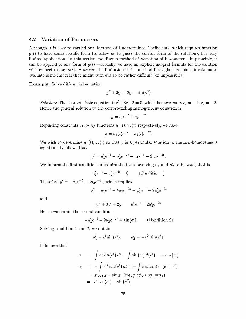
4.2 Variation of Parameters

Although it is easy to carried out, Method of Undetermined CoeÆcients, which requires function

g(t) to have some speci�c form (to allow us to guess the correct form of the solution), has very

limited application. In this section, we discuss method of Variation of Parameters. In principle, it

can be applied to any form of g(t) { actually we have an explicit integral formula for the solution

with respect to any g(t). However, the limitation if this method lies right here, since it asks us to

evaluate some integral that might turn out to be rather diÆcult (or impossible).

Example: Solve di�erential equation

y00 + 3y0 + 2y = sin

�ex�

Solution: The characteristic equation is r2+3r+2 = 0, which has two roots r1 = �1, r2 = �2.Hence the general solution to the corresponding homogeneous equation is

y = c1e�t + c2e

�2t

Replacing constants c1; c2 by functions u1(t); u2(t) respectively, we have

y = u1(t)e�t + u2(t)e

�2t:

We wish to determine u1(t); u2(t) so that y is a particular solution to the non-homogeneous

equation. It follows that

y0 = u

01e�t + u

02e�2t � u1e

�t � 2u2e�2t

:

We impose the �rst condition to require the term involving u01 and u02 to be zero, that is

u01e�t + u

02e�2t = 0 (Condition 1)

Therefore y0 = �u1e�t � 2u2e�2t, which implies

y00 = u1e

�t + 4u2e�2t � u

01e�t � 2u02e

�2t

and

y00 + 3y0 + 2y = �u01e�t � 2u02e

�2t

Hence we obtain the second condition

�u01e�t � 2u02e�2t = sin

�et�

(Condition 2)

Solving condition 1 and 2, we obtain

u01 = e

t sin�et�; u

02 = �e2t sin

�et�:

It follows that

u1 =

Zet sin

�et�dt =

Zsin�et�d�et�= � cos

�et�

u2 = �Ze2t sin

�et�dt = �

Zx sinx dx (x = e

t)

= x cos x� sinx (integration by parts)

= et cos

�et�� sin

�et�

25

Therefore, a particular solution is

yp = �e�2t sin�et�

The general solution is

y = c1e�t + c2e

�2t � e�2t sin

�et�:

Let us now give a general description of this method. Consider di�erential equation

y00 + p(t)y0 + q(t)y = g(t)

and suppose that y1; y2 is a fundamental set of solutions to the corresponding homogeneous equation

y00 + p(t)y0 + q(t)y = 0;

whose general solution is therefore y = c1y1 + c2y2.

Replace constants c1; c2 by functions u1(t); u2(t). We wish to determine u1; u2 so that

y4= u1y1 + u2y2

is a particular solution to the non-homogeneous equation. Observe

y0 = u

01y1 + u

02y2 + u1y

01 + u2y

02:

We impose the �rst condition to erase the terms involving u01; u02:

u01y1 + u

02y2 = 0 (condition 1)

Hence y0 = u1y01 + u2y

02, y

00 = u02y01 + u

02y02 + u1y

001 + u2y

002 , and

y00 + p(t)y0 + q(t)y = u1

�y001 + p(t)y01 + q(t)y1

�+ u2

�y002 + p(t)y02 + q(t)y2

�+ u

02y01 + u

02y02:

We obtain our second condition

u02y01 + u

02y02 = g(t) (condition 2)

Solving condition 1 and 2, we have

u01 = �y2g

W; u

02 =

y1g

W

where W is the Wrondskian of y1 and y2. Therefore, a particular solution is

yp = �y1Z

y2g

W+ y2

Zy1g

W

and general solution is

y = c1y1 + c2y2 + yp:

Exercise: Find the general solution of equation

y00 + 4y0 + 4y = 3xe2x

using both methods of Undetermined CoeÆcients and Variation of Parameters.

26

4.3 Reduction of Order (revisited)

Suppose we have been able to �nd a nontrivial solution y1 to the homogeneous equation

y00 + p(t)y0 + q(t)y = 0:

It is already shown that by the reduction of order method we shall obtain a second linear inde-

pendent solution to this homogeneous equation, and thus the general solutions. Here we show that

by this method we shall also be able to obtain from y1 the general solutions of a non-homegenous

equation

y00 + p(t)y0 + q(t)y = g(t):

The basic procedure remains the same. Assuming that y2(t) = v(t)y1(t) is a second solution, we

have

y02 = v

0y1 + vy

01; y

002 = v

00y1 + 2v0y01 + vy

001

and

v00y1 + 2v0y01 + vy

001 + p(t)v0y1 + p(t)vy01 + q(t)vy = g(t) ) y1v

00 +�2y01 + p(t)y1

�v0 = g:

Letting w4= v

0, we obtain a �rst order di�erential equation

y1w0 +�2y01 + p(t)y1

�w = 0

This is now a linear equation and can be solved by �nding the integrating factor.

Example: Given y1 = t is a solution to equation

t2y00 + ty

0 � y = 0; t > 0;

�nd the general solution of the non-homogeneous equation

t2y00 + ty

0 � y = t; t > 0:

Solution: Let y2(t) = v(t)y1(t) = tv(t). We have

y02 = tv

0 + v; y002 = tv

00 + 2v0

Substituting this in the non-homogeneous equation gives

t2(tv00 + 2v0) + t(tv0 + v)� tv = t ) t

3v00 + 3t2v0 = t:

Let w = v0, we have

t3w0 + 3t2w = t ) (t3w)0 = t ) t

3w =

1

2t2 + c

or

w =1

2t+

c

t3) v =

Zw dt =

1

2ln t� c

2t2+ c

0

which is equivalent to

y2(t) =1

2t ln t� c1

t+ c2t:

This is the general solution of the non-homogeneous equation.

27

Exercise: Given y1(x) = x2 is a solution to the homogeneous equation

x2y00 � 2y = 0:

Find the general solution of non-homogeneous equation

x2y00 � 2y = 2x:

(Answer: y = c1x2 + c2

x+ 2

3x2 lnx)

5 Vibrations and Equibilirium

Newton's Law of Motion says F = ma, where m is the mass of the particle, a is its acceleration,

and F is net external force.

5.1 Free Motion

Here we shall consider two applications of second order linear equation to physics.

Example 1 (Elastic Spring. Hooke's Law): Suppose a mass m is attached to a verticle spring

whose unstreched length is l. This mass is subject to two forces: its own weight mg, and force

due to spring Fs. It follows from Hooke's Law, with the positive direction taken as downward,

Fs = �ky:

Here the positive constant k is called spring constant.

1. Undamped Free Vibration: Assuming for a moment that there is no damping force (e.g.

air resistance), the net external force is therefore

F = mg + Fs = mg � ky (g is the accerlation due to gravity)

which implies, by Newton's Law,

F = mg � ky = ma = m�y ) �y +k

my = g:

Equilibrium Position: By letting �y = 0, we obtain the equilibrium position

y� =

mg

k:

At equilibrium position y�, the mass has a net external force F = mg � ky

� = 0.

28

Let u4= y � y

� (deviation from equilibrium). It is easy to see that u satis�es equation

�u+k

mu = 0;

which has general solution, with !04=

qkm

u = c1 cos!0t+ c2 sin!0t = R cos(!0t� Æ):

Here reparametrization R; Æ are determined as before by

R =

qc21 + c22; cos Æ =

c1

R; sin Æ =

c2

R:

It is easy to see that R is the maximal deviation from the equilibrium.

Terminology: The parameters !0, R and Æ are called natural frequency, amplitude, and

phase respectively. T4= 2�

!0is called period.

Example: A 2-pound mass attached to a spring stretches it 4 inches. If the mass is

displaced an additional 4 inches and is released. Determined the position of the

mass at time t.

Solution: We �rst determine the mass m by

m =mg

g=

2 lb

32 ft=sec2=

1

16

lb-sec2

ft

Since equilibrium position y� = mg

k= 2, we obtain

k =mg

4-in=

2 lb13ft

= 6lb

ft

Let u be the deviation from equilibrium. We have equation

0 = �u+k

mu = �u+ 96u;

which hasgeneral solution u = c1 cosp96t+ c2 sin

p96t. The initial conditions are

u(0) = 4 in =1

3ft; u

0(0) = 0;

which yield c1 =13, c2 = 0, or

u =1

3cos

p96t:

The amplitude is R = 13-ft, phase Æ = 0, natural frequency !0 =

p96 = 9:8 radsec

(hence the period is T = 2�!0

= 0:64-sec). 2.

29

2. Damped Free Vibration: Now let us take the damping force Fd into consideration. Sup-

pose the mass is also subject to a damping force proportional to its velocity,

Fd = � u0(t):

Here > 0 is the constant of proportionality. The equilibrium position will NOT change.

The net external force is therefore

mu00 = ma = F = mg � k(y� + u)� u

0 ) mu00 + u

0 + ku = 0

here u is the deviation from the equilibrium like before. The corresponding characteristic

equation is

mr2 + r + k = 0 ) r1;2 = �

2m�p 2 � 4km

2m:

There are three cases.

1. Overdamped ( > 2pkm): In this case, r1;2 are both real and negative (check!).

The general solution is

u = Aer1t +Be

r2t

It is easy to see that the motion is non-oscillatory (see graph below). Moreover, as

t!1, the deviation will diminish.

2. Critically damped ( = 2pkm): In this case, r1;2 = r = �

2mis real and negative.

The general solution is

u = Aert +Bte

rt:

Like in the overdamped case, the motion is non-oscillatory and diminishes as t!1.

The graphes are also similar to the overdamped case.

3. Underdamped ( < 2pkm): In this case, r1;2 are conjuate complex numbers with

negative real parts. The general solution is

u = e�

2mt�A cos�t+B sin�t

�= Re

� 2m

t cos(�t� Æ):

Here �4=

p4km� 22m

> 0, and R; Æ are determined by A = R cos Æ;B = R sin Æ.

Clearly the motion is oscillatory (but not periodic), and diminishes as t ! 1. It

has a damped amplitude Re�

2mt, which goes to zero as t ! 1. See the following

graph.

30

Qunatities � =

p4km� 22m

and T4= 2�

�are called quasi-frequency and quasi-period

respectively.

Example 2 (Archimedes' Principle): Archimedes' Principle states that a body submerged in

a uid is subjected to an upward (buoyant) force with magnitude equal to the weight of

displaced uid.

Floating in a liquid is a l ft high cylindrical body with cross-sectional area S (sq ft). The

mass densities of the body and the liquid are � and �̂ per unit volume, respectively. Assume

r4= �

�̂< 1 (otherwise, the body will sink), and neglect viscous damping forces. Let y stand

for the distance from bottom of the body to the surface, with the positive direction taken

as downward. The body has mass m = �lS, while the displaced liquid has mass m̂ = �̂yS.

Therefore, the net force on the body is

F = mg � m̂g = Sg(�l � �̂y) ) y00 =

F

m=

F

�lS= g

�1� y

rl

�We obtain immediately the equilibrium position y

� = rl.

Let u4= y � y

� be the deviation from the equilibrium. It follows that u satis�es equation

u00 +

g

rlu = 0:

Even though this is a very di�erent physics problem, we end up with same type of di�erential

equation. All the properties we have obtained in the spring example hold in this case. We

leave the details to the interested students.

Exercise: Show that the period for the body motion is

T = 2�

srl

g:

5.2 Forced Motion

In this section, we will only consider the undamped motion. Interested readers can �nd more

details in the textbook. Suppose now a periodic external force, say F = F0 cos!t, is imposed to

the system. Here ! is the frequency of the external force.

Elastic Spring (continued): Let u = y � y� be the deviation from equilibrium. We have

mu00 + ku = F0 cos!t:

Exercise: Show that, with u04=

qkm

as the natural frequency,

up4=

�; if !0 6= !

F02m!0

t sin!0t ; if !0 = !

is a particular solution to the di�erential equation. Hence the general solution takes

form

u = c1 cos!0t+ sin!0t+ up:

31

>From the form of up, we discuss the motion according to !0 6= ! or !0 = !.

!0 6= !: In this case, the resulting oscillation of the body is the sum of two periodic displacements

with di�erent frequencies, namely !0 and !. It is said to be a stable motion in the sense that

the deviation remains bounded. This motion, however, might be non-periodic. Actually it is

periodic if and only if !0!

is a rational number.

!0 = !: (Resonance) The presence of variable t in the particular solution implies that the deviation

goes unbounded as t!1 (hence an unstable motion). In such cases, a mechinal breakdown

of the system is bound to occur. This phenomenon, where the frequency of external force

equals the natural frequency of system, is known as (undamped) resonance.

6 Weak Maximum Principle

Weak Maximum Principle: Suppose y satis�es the following di�erential inequality

y00 + p(t)y0 � 0; a � t � b

where p(t) is continuous on interval [a; b]. Show that

maxt2[a;b]

y(t) = maxfy(a); y(b)g

That is, the maximum of y is achieved at the boundary of the interval.

Proof: To ease exposition, let

L[y]4= y

00 + p(t)y0:

For any constant �, we have

L[e�t] = e�t(�2 + p(t)�):

Since p(t) is continuous on interval on interval [a; b], it must be bounded. Fix any � >

maxt2[a;b] jp(t)j, we haveL[e�t] = e

�t(�2 + p(t)�) > 0

for all t 2 [a; b]. Hence, for any " > 0, let u" = y + "e�t. We have

L[u"] = L[y + "e�t] = L[y] + "L[e�t] > 0:

for all t 2 [a; b]. We claim that

maxt2[a;b]

u"(t) = maxfu"(a); u"(b)g:

Otherwise, there exist c 2 (a; b) such that u" achieves maximum at t = c. However, this

implies u0"(c) = 0 and u00"(c) � 0, or

L[u"](c) = u00"(c) + p(c)u0"(c) = u

00"(c) � 0;

a contradiction.

Now letting "! 0, we have u" ! y uniformly on interval[a; b]. Therefore

maxt2[a;b]

y(t) = maxfy(a); y(b)g

This completes the proof. 2

32

From now on we will let L[y]4= y

00 + p(t)y0. We have the following comparison principle. Note

the di�erence here is that the initial conditions are the initial values of the solution at the two

end-points.

Comparison principle: Suppose L[y] � L[z] for all t 2 [a; b] and y(t) � z(t) for t = a; b (bound-

ary of the interval). Then y(t) � z(t) for all t 2 [a; b].

Proof: Let w4= y � z. We have

L[w] = L[y]� L[z] � 0; w(a) � 0; w(b) � 0:

Therefore, by the weak maximum principle, we have

maxt2[a;b]

w(t) = maxfw(a); w(b)g � 0:

This completes the proof. 2

Corollary (Uniqueness): The initial value problem

L[y] = 0; t 2 [a; b]

with initial condition y(a) = y0; y(b) = y1 has at most one solution.

Proof: Suppose y and z are both the solution to the above initial value problem, we have

L[y] = L[z]; y(a) = z(a); y(b) = z(b):

It follows that y � z and y � z for all t 2 [a; b] (Comparison principle). Therefore y(t) � z(t)

for all t 2 [a; b]. 2

Remark: the comparison principle and uniqueness hold for more general linear operator

L[y] = y00 + p(t)y0 + q(t)y

where q(t) � 0. One can derive this general comparison principle from weak maximum

principle, which is not terribly diÆcult.

7 Non-linear Second order ODE

Consider the following general nonlinear initial value problem of second order

y00 = f(t; y; y0); t 2 I:

with initial condition y(t0) = y0; y0(t0) = z0. We have the following fundamental theorem regarding

the existence and uniqueness of the solution.

Theorem: If functions f(t; y; z), fy(t; y; z) and fz(t; y; z) are continuous in region

R =�(t; y; z)

Æjt� t0j � a; jy � y0j � b; jz � z0j � c

;

33

then there exists a unique solution y = �(t) of the initial value problem

y00 = f(t; y; y0); y(t0) = y0; y

0(t0) = z0

on an interval jt� t0j � h for some h � a.

Proof: Let z4= y

0, we have the equivalent system of �rst order equations�y0 = z

z0 = f(t; y; z)

Write

W =

�y

z

�; F (t;W ) =

�z

f(t; y; z)

�:

We havedW

dt= F (t;W ); W (t0) =

�y0

z0

�Using the same iteration method as for the �rst order ODE and the Gronwall inequality,

the existence and uniquess of the solution W = �(t) = [�1(t);�2(t)]t follows. Therefore

�(t) = �1(t) is the solution to the original second order initial value problem. 2

In the following, we will collect miscellaneous problems and examples.

Boundedness: Suppose y solve the di�erential equation

y00 + V

0(y) = 0; t 2 IR

where V is a smooth function on IR with

limz!�1

V (z) =1:

Show that y is bounded.

Proof: Multiplying both side by y0, we have

y0y00 + V

0(y)y0 = 0 ) d

dt

�1

2(y0)2 + V (y)

�= 0

or1

2(y0)2 + V (y) = c

for some constant c. However, this implies that V (y) is bounded from above by the constant

c. Since limz!�1 V (z) =1, we must have that y(t) is bounded. 2

Remark: The above method also provides a way to solve the type of di�erential equation

y00 + V

0(y) = 0:

We should have

1

2(y0)2 + V (y) = c ) y

0 = �q2�(c� V (y)

�) dyq

2�(c� V (y)

� = �dt

34

The following are two example of the applications of the nonlinear di�erential equation of second

order: populations of two interacting species and Newton's law of universal gravitation.

A biological problem: There is a constant struggle for survival among di�erent species. For

example, certain birds live on �sh. If there is an abundant supply of �sh, the population

of this bird species grows. When these birds become too numerous and consume too much

�sh, thus reducing the �sh population, then their own population begins to diminish. When

the number of birds decreases, the �sh population increases, then the bird population starts

increasing. This induces an endless cycle of periodic increases and decreases in the respective

populations of the two species.

We will consider the problem of determining the populations of two interacting species: a

parasitic species P hatches its eggs in a host species H. Unfortunately, the deposit of an egg

in a member of H causes this member's death. Let

1. Hb denote the birth rate for the H species.

2. Hd denote the (natural) death rate for the H species, if no P species were present.

3. Pd denote the (natural) death rate for the P species.

Suppose (x; y) denote the population size for H and P species, respectively. Also assume that

the number of eggs per year deposited by the P species is propotional to the probability that

the members of the two species meet. Since this probability depends on the product xy of the

two population size, we assume that, in time 4t, the approximate number of eggs deposited

on H species is kxy4t. We have

4x = Hbx4t�Hdx4t� kxy4t4y = kxy4t� Pdy4t:

Letting h = Hb �Hd, p = Pd and 4t! 0, we have

x0 = hx� kxy = x(h� ky)

y0 = kxy � py = y(kx� p):

This is a system of �rst order di�erential equations. It is possible to solve y as a function of

x. Actually,

dy

dx=

y0

x0=

y(kx� p)

x(h� ky))

�h

y� k

�dy =

�k � p

x

�dx;

which leads to, for some constant c,

ln�cy

hxp�= k(x+ y) ) cy

he�ky = x

�pekx

If x(0) = x0; y(0) = y0, then one can determine

c = x�p0 y

�h0 e

k(x+y):

However, such an implicit solution might not be intuitive to deal with.

35

We will give an approximation of the system (linearization of �rst order systems). The

equilibrium solution to this system is

h� ky� = 0; kx

� � p = 0 ) y� =

h

k; x

� =p

k

Use the change of the variable,

x = x� +X; y = y

� + Y:

We have (check!)dX

dt= �pY � kXY;

dY

dt= hX + kXY:

However, if the deviations from the equilibrium (X;Y ) is small, we may, without serious error,

discard the XY term. These equations then become

dX

dt= �pY; dY

dt= hX ) dY

dX= �hX

pY:

It follows thatX

2

p+Y

2

h= c

for some constant c. The graph is an ellipse (when h = p, it is a circle). 2

New's inverse square law: Kepler's three laws of planetary motion are:

1. The planet moves in an elliptical orbit with the sun at one focus.

2. The radius vector connecting sun and the planet sweeps out equal areas in equal times.

3. The square of the period of the planet's movement is proportional to the cube of the

semimajor axis of its orbit (a in the graph).

36

Newton's law of universal gravitation states that: if M and m are the mass of two planets,

then the two bodies attracts each other with a central force

F = �GMm

r2:

Here r is the distance between the two planets.

In the following, we are going to derive (partially) the Newton's law from Kepler's �rst two

laws. Indeed we are going to show that F is a central force inversely proportional to the

square of the distance r.

Proof: We will divide the proof into several steps.

Step 1: We are going to use the polar coordinates (r; �) to denote the position of the planet

(see the graph). It follows from analytical geometry that

r =c

1 + k cos �

for some constant c and some constant k < 1. The constant k is called eccentricity (indeed,

if k = 1, this equation corresponds to a parabola; if k > 1, it corresponds to a hyperbola).

Here we give a short proof. We have

r + �r = constant := l ) r +p(r sin �)2 + (r cos � + d)2 = l;

which implies

(l � r)2 = r2 + 2rd cos � + d

2 ) l2 � d

2 = r(2l + 2d cos �) ) r =l2�d22l

1 + dlcos �

But k = dl< 1. This completes the proof.

Step 2: Suppose at time t, the planet is at position�r(t); �(t)

�. The speed and acceleration

of the body can both be decomposed into two components: one along the radius r, the other

in a direction perpendicular to it (see the graph below). We claim

vr = r0; v� = r�

0; ar = r00 � r(�0)2; a� = 2r0�0 + r�

00:

37

Actually, since x = r cos �; y = r sin �, we have

speed along x-axis = x0 = cos � � r0 � sin � � r�0 = cos � � vr � sin � � v�

speed along y-axis = y0 = sin � � r0 + cos � � r�0 = sin � � vr + cos � � v�

which clearly implies that vr = r0; v� = r�

0: Similarly,

accleration along x-axis = x00 = cos � �

�r00 � r(�0)2

�� sin � � (2r0�0 + r�

00) = cos � � ar � sin � � a�accleration along y-axis = y

00 = sin � ��r00 � r(�0)2

�+ cos � � (2r0�0 + r�

00) = sin � � ar + cos � � a�

which gives ar = r00 � r(�0)2; a� = 2r0�0 + r�

00.

Step 3: By Kepler's second law, if we denote A(t) the area that the radius vector connecting

sun and the planet sweeps up to time t, we have dAdt

is a constant, say p

2. However, dA = 1

2r2d�

(why?), which implies that

r2d�

dt= p ) 2rr0�0 + r

2�00 = 0 ) 2r0�0 + r�

00 = 0:

In other words, the acceleration perpendicular to the radius a� equals 0. Since this component

is zero, the force acting on the planet must be a central one.

Step 4: As we have already seen, the equation for an elliptical orbit in polar coordinates is

r =c

1 + k cos �

for some constant c and eccentricity e. We have

r0 =

ce sin �

(1 + k cos �)2�0 = r

2k sin �

c

p

r2=pk

csin �:

Therefore

r00 =

pk

ccos � � �0 = p

2

cr2(k cos �) =

p2

cr2

�c

r� 1�:

The last equality follows from the equation for the ellipse. The component of the force in the

radius direction is

Fr = mar = m�r00 � r(�0)2

�= m

�p2

r3� p

2

cr2� r

p2

r4

�= �mp

2

cr2:

This completes the proof. 2

38