in the relationship between broad money and stock … · the relationship between broad money and...
TRANSCRIPT
12
In 1:
in
os k.
J"rnal Ekonomi Malaysia 32 (1998) 51·73
The Relationship between Broad Money and Stock Prices in Malaysia: An Error Correction Model Approach
Muzafar Shah Habibullah
ABSTRAK
Tujuan kajian in; ada/ah Ullluk menyelidik hubungan empirik amara penawarall wang dan harga-harga saham di Bursa Saham Kuala Lumpur (KLSE) dengan menggunakan data bulanan yang merangkumi Januari 1984 hingga September 1992. Khususnya, kecekapan pasaran terhadap penerimaan maklumat di Bursa Saham Kuala Lumpur diuji dengan melihat hubungan sehab Qntara penawaran wang. M3. dan harga-harga saham dengan teknik 'cointegration.' Hasil daripada 'Error Correction model ' mencadangkan bahawa hiporesis kecekapan pasarall terhadap penerimaan maklumat bolell ditolak untuk Bursa Saham Kuala Lumpur.
ABSTRACT
The purpose of this study is to investigate the empirical relationship beTween money supply and stock prices in the Kuala Lumpur Stock Exchange (KLSE), using mowhly data that span from January 1984 to September 1992. Specifically, we test for market infonnational efficiency in KLSE by testing the causal relationships benveen money supply, M 3 and stock prices using the cointegration techn ique. Results from Ollr Error Correction models suggest that the informational efficiency markets hypothesis can be rejected for the KLSE.
INTRODUCTION
Following the work of Sprinkel ( 1964), several studies have attempted to test statistically the react ion of the stock market to growth in money supply. The money supply-stock market nexus has been widely tested because of the belief that the growth in money supply has important
52 Jumal Ekonomi Malaysia 32
direct effects through portfolio changes, and indirect effects through their effects on real activity variables, which in turn postulated to be the fundamental detenninants of stock prices. Nevertheless, given the importance of money in the detennination of stock prices, an important question that arises pertains to the efficiency with which stock market part ic ipants incorporate the information contained in the growth of money supply into stock prices. This question is important because if the market is inefficient with respect to the re levant information, then investors can earn consistently higher than normal rates of re turn. Furthennore, it raises serious doubts about the ability of the stock market to perform its fundamental role of channelling funds to the most productive sectors of the economy.
Secondly and more importantly is the following question ; Do different measures of money supply yield different effects on stock prices? Kraft and Kraft (l977a, 1977b) conclude that the detection of lead-lag relationship between money supply and stock prices are insensitive to the choice of the definition of money supply used. However, seve ral other empiri cal studies have shown that different choices of money supply measures can have different impacts on stock prices. A brief summary of the impact of alternative definitions of money supply used on stock prices in the recent money supply-stock market nexus is presented in Table I. We can clearly see from Table I that the presence (or the absence) of lead-lag relationships between money supply and stock prices are sensitive to the choice of the definition of money supply used. For example, take the case of Mookerjee's (1987) study, where for Canada, the stock market is efficient with respect to narrow money supply M I , but with broad money supply M2, the resul ts suggest that money supply is the leading indicator for stock price. Resuits from Thornton (1993), Ho (1983) and Jones and Uri (1987) tend to point to the conclusion that stock markets are sensitive to different measures of money supply used. Therefore , we can conclude that different measures of money supply used can yield different impacts on the stock prices.
In this study, we want to determine whether broad money supply M3 can be a leading indicator for the stock prices in Malays ia. Although the Central Bank of Malaysia has given greater emphasis on the use of broad money M3 as guide for monetary policy purposes, nevertheless the effectiveness of M3 as a monetary instrument is still subject to empirical verification (Bank Negara Malaysia 1990). For example, in a recent study, Ghosh and Gan ( 1994) queried the role of broad money
~
(

32 Broad Money arid Srock Prices 53
;!Ir M3 as monetary instrument and they concluded that the broad concept
he (M3) does not serve well with the Malaysian economy. Instead the more
he re levant stock of money seems [Q be the conventional and narrow one
tnt (M I).
~et
of TABLE I. Summary of previous studies on money supply and stock market if relationships
en "11. Authors Period of study Money Countries Conclusions
:et Mookerjee Monthly MI France, USA, >S t (1987) (1975: 1-1985:3) Germany,
Netherlands. Independent )0
ok Japan, Italy, Unidirecti onal
of Switzerland. M~S
re Canada. Unidirecti onal d. S~M
nt ok UK Bidirect ional
of M=S
ok M2 France, USA
Germany, 'n Switzerland. Independent fi- Japan , Italy. !'S
:c1 Canada. Unidirectional M~S ,e
:e. UK. Netherlands Unidirectional ,d S~M
nt .at Quarterl y MI France, USA,
)n (1975: 1-1985:1) Japan, Switzerland. Netherland, UK,
Iy Germany. Belgium. Independent
~h Italy. Unidirectional
of M~S
ss to Canada Unidirec lionai
S~M In
'y cominued next page

54 iumal £konomi Malaysia 32
Table I (Continued) s
Authors Period of study Money Countries Conclusions ~
M2 France, USA, Japan, Switzerland, a
Netherland, f Gennany, Belgium. Independent tl
e Italy, Canada. Unidirectional t
M--.S s
UK Unidirectional n S--.M e
tl Ho (1983) Monthly MI Hong Kong. Independent d
(1975:1-1980:12) Australia, Singapore, d
Thailand. Bidirectional e:
M=S H aJ
Japan, Unidirectional Philippines. M--.S r<
M2 Singapore. Bidirectional IT
M=S el
Australia, pI Hong Kong. Japan. w Philippines, Unidirectional u: Thailand. M--.S di
Monthl y MO USA. Unidirectional Fi
(1974:5-1983: 1 0) M--.S
M
MI USA. Unidirectional M--.S TI
M2 USA. Independent TI to
Quarterly MO UK. Independent de (1963:1-1990:4) Fe
cr' M5 UK. Unidi rectional
S--.M pr
'"' pr

32
• 1
1
Broad Money and Slock Prices 55
The concl usion arrived by Ghosh and Gan (1994) is not without support. Habibullah ( 1992) investigated the effec tiveness of money M I , M2 and M3 as a result of financial sophistication and financial innovations in Malaysia by testing the Gurley-Shaw hypothesis. Gurley and Shaw (1960) hypothesised that the presence of interest-bearing financial assets offered by non·bank financial intermediaries will increase the interest rate elasticity of money demand and consequently hinder the effectiveness of M I , M2 and M3 for monetary policy purposes . Habibullah ( 1992) fou nd that the Malaysian monetary data did not support the Gurley-Shaw contention that changes in the financial markets and the growth of money substitutes will increase the interest elasticity of money demand for MI , M2 and M3. This result implies that money supply M I, M2 and M3 has been stable for the period under study and the Central Bank of Malaysia may have used all three definitions of money supply for monetary policy purposes. Therefore, excluding M 1 for monetary management is unwarranted. In other words, Habibullah's ( 1992) study indicated that money supply MI , M2 and M3 are equally good monetary instruments in Malaysia.
Therefore , the primary purpose of this study is to invest igate the relationship between broad money supply M3 and stock prices using monthly data. Specifically, this study tests for market informational efficiency in Malaysia by testing the causal relationship between stock prices and money supply using the cointegration approach. In this study we use a broader definition of money supply, that is, M3. Apart from using the Composite stock price index , in this study we also use disaggregated data for stock price indexes, namely; Industrial, Plantation, Finance, Property and Tin.
METHODOLOGY
THE GRANGER CAUSALITY APPROACH
Traditionally, the causality tes t developed by Granger ( 1969) is used to test the informational effic iency of the stock market. Granger's definition of causality relies on the predictability of a time series. Formally. the above proposi tion can be stated as fo llows: if cr'(xlx.y)<cr'(xlx), then y is said to cause x. The term cr'(xlx.y) is the prediction error variance of x derived from the information set that includes past va lues of x and y. The term cr'(xlx) is the variance of the prediction error of x based on inform ati on contained onl y in the past

56 Jurnal Ekonomi Malaysia 32
values of x. If, however, cr'(y/y.x)<cr' (y/y) then x is said to cause y. Bidirectional causality is said to occur when the above outcomes occur simultaneously. Finally, if cr'(xlx)<cr'(xlx,y) and cr'(y/y)<cr'(y/y,x), then the two series are not temporally related over time and are therefore independent.
A direct test of Granger causality between stock prices (S) and money supply (M) amounts to estimating the following equations
(I)
(2)
where Il" and Il" are independent, and E[Il",ll h]=O, E[Il'" Il'.]=O, and E[Il I',Il'.]=O, for all t;<s.
From equations (I) and (2), unidirectional causality from stock prices to money supply can be established if the estimated coefficients on the Jagged stock price variables are significantly different from zero in equation (I), and the estimated coefficients on the lagged money supply variables as a group are not significantly different from zero in equation ( I). This finding would imply stock market informational efficiency.
Causality from money to stock prices would be implied if the estimated coefficients on the lagged money supply variables as a group are significantly different from zero in equation ( I) , and the coefficients of the lagged stock price variables as a group in equation (2) are not significantly different from zero. This finding would suggest stock market infonnational inefficiency.
If, however, the estimated coefficients of the lagged variables of both stock price and money supply as a group in equation, ( I) and (2) are significantly different from zero, then bidirectional causality is implied between stock prices and the money supply. This fi nding would also imply stock market inefficiency.
Finally, if the estimated coefficients on the lagged variables of both stock price and money supply as a group in equations ( I ) and (2) are not significantly different from zero, then no causal ity is implied between stock price and money and the two series are not temporally re lated to each other and are independent. This finding would imply stock market effic iency.
B
T
V tl tI fi C tl 11
n n
fi S a·
" " c. f!,
e: o
el t(
b o C IT
a

2
r
Broad Money and Srock Prices 57
THE ERROR CORRECTION MODEL AP PROACH
When estimating equations (1) and (2), the series are required to be in their stationary fonn. Conventionally, the variables are transformed in their first-difference form in order to induce stationarity or using some filter rule as suggested by Box and Jenkins (1970). Furthermore, Granger and Newbold (1977) have pointed out that the danger in using the first-difference form of the data is that potential valuable long-run information contained in the variable expressed in levels are lost. More recently, Engle and Granger (1987) have demonstrated that if two non-stationary variables are cointegrated, a vector autoregression in the first-difference is misspecified. It was shown in Granger (1988) that, if St, Mt are both 1(1), but are cointegrated then they will be generated by an Error Correction model of the following form;
(3)
(4)
where one of al, e~:;C{) and Ell, E2l are finite-order moving averages. Thus, in the Error Correction ModeL there are two possible sources of causation of SI by M L-I either through the Zl-I lerm , if 81~, and through AMI term if they are present in the equation. Without ZI_] being expl icitly used, the model will be mis-specified and the possible value of lagged MI in forecasting St will be missed.
Rewritin g equations ( I) and (2) in order to take into account the error correction term, we have the following Error Correction model due to Granger ( 1988),
K ]'I
6S, = a. + L .. , u ;6S,.; + L,., ~,6M. ., - 8,zl.l. , +~" (5)
K N 6M, = yo + L;., y,6S,., + L,., O,6M,., - 8,z).,., + ~ " (6)
where ZI_] is the lagged residuals from the cointegration regression between stock price and money supply in level. Granger (1988) pointed out that , based on equation (5), the null hypothesis that M does not Granger cause S is rejected not only if the coefficients on the lagged money supply variables are jointly significantly different from zero, but also if the coefficient on ZI.l is significant. The Error Correction

58 iumal Ekonomi Malaysia 32
Model also provides for the finding that M Granger cause S, if ~.I is significant even though the coefficients on lagged money supply variables are not jointly significantly different from zero. Furthennore, the importance of a 's and Ws represent the short-run causal impact, while e gives the long-run impact. In determining whether S Granger cause M, the same principal applies with respect to equation (6).
The concept o f cointegration was firs t introduced by Gran ger (1981). The cointegration methodology provides a way in which the long run information of the integrated series in level is conserved in to equations that comprise stationary components called the error correction model that gives valid statis tical inferences. For any 1(1) series. it is always true that the linear combination of the two series will also result in an I(l ). However, if there exists a constant A. such that z,=S,-AM, is stationary or 1(0), then S, and M, will be said to be cointegrated. with A called the cointegrating parameter. If this were not the case, then the variables assumed LO be generating the equilibrium can drift apart without bound, which is contrary to the equilibrium concept. If S, and M, are 1(1 ) but coi ntegrated, then the relationship S,=AM, is considered a long run or 'equilibrium' relationship, and Zt given above measure the extent to which the system SI, Mt are out of equilibrium (Granger 1986). Hence, the existence of a linear combination of two I( I) series that is 1(0) suggests that the series generally move together over time, such that the relationship holds in the long run .
DATA USED IN THE STUDY
In this study, we used monthly time series data for the Kuala Lumpur Stock Exchange (KLSE) stock price indices, namely the Composite, Industrial. Finance, Property, Plantation and Tin srock indexes. The KLSE stock indices were collected from various issues of the Investors Digest published monthly by KLSE. On the o ther hand, money suppl y M 3 comprised of currency in circulati"n and demand deposits held by non-bank private sector; savings deposits, fixed deposits. negotiable certificate of deposits and repos at commercial banks, finance companies, Bank Islam, merchant banks and discount houses. Data on M3 are taken from various issues of Quarterly Bulletin published by Bank Negara Malaysia. In this study the data used spans from January 1984 until September 1992. All data used in the analysis is are transformed into natural logs.
E
E tl v
c tI \I
a
" c.
h tt \I
a' c, c p
(~
al C1
w
a Z<
cr In
I S

2
s y
e e
r
)
r
S
1
1
r
Broad Money and Srock Prices 59
EMPIRICAL RESULTS
Before we estimate equations (I) and (2), we have to determine whether the z.., terms in equations (5) and (6) are valid or nol. To ascertain the validity of the Zt-l term, we estimate the cointegrating regressions comprises of the two variables, that is, S, and M,. If the residual z, of the linear combination of S, and M, is 1(0), then Z,., should be included in Equations ( I) and (2) and therefore Equations (5) and (6) is appropriate for the Granger causality testing. If on the other hand, zt is not 1(0), then Equations ( I) and (2) is the appropriate Granger causality testing approach.
However, before the cointegrating regress ions can be estimated, we have to determine the order of integration of the series of interest. In this study we employed unit root tests to determine the order of integration of the individual series. Thi s is because only variables that are of the same order of integrari on may constitute a potential cointegrating relati onship. In this study we employed the Augmented Dickey and Fuller ( 1981) unit root tesl. The test is the t-statistic on parameter a of the following equation
(7)
where VI is the disturbance term. The role of the lagged dependent variables in the Augmented Dickey-Fuller (ADF) regression equation (7) is to ensure that Vt is white noise. Thus, we have to choose the appropriate lag length L In this study we used Schwer!'s ( 1987, 1989) criteria which is given by the following two formulations ;
L, = int(4(TIl00)'''} and L,,=int{ 12(TIlOO)' '' } (8)
where T is the total number of observations.
The null hypothesis, Ho: S, is I( I ), is rejec ted (i n favour of 1(0)) if a is found to be negative and statistically significantly different from zero. The computed t~stati sti c on parameter a, is compared to the critical value tabulated in MacKinnon (199 1). If a time trend is also inc luded in equation (7), we have the following equation (9) which is used to derer.nine wh~lher the series is trend·stati onary (TS),

60 iumal Ekonomi Malaysia 32
L 6 S, = 00 + e. + ~S'.I + L ;'I &6S,.; + t, (9)
where t is a time trend . If parameter ~ is negative and significantly different from zero then 51 is said to be trend-stationary. The difference between a di fference-stationary process (osp) and a trend-stationary process (TS P) is that , th e fo rmer requires diffe re ncin g to ac hieve stationarity (Dickey & Fuller 1979). However, for TSF, stationarity is achieved by inclusion of a time trend variable. It is important to check for the correct form of non-stationary behaviour of the time series because a difference-stationary process which is stochastic cannot be cointegrated with a trend-stationary process which, on the other hand, deterministic. Nelson and Plosser (1982) have demonstrated that many economic time series appear to be difference-stationary processes .
The unit root tests were also carried out for first-difference of the variable, that is, we estimate the fo llowing regression equation;
(10)
where the null hypothesis is Ho: S, is 1(2), which is rejected (in favour of 1(1) if a is found to be negative and statistically significantly different from zero.
Table 2 presents the results of the unit root tests on the levels and first-difference of the series. Following Schwert (1987. 1989), the truncation lag length chosen was based on the integer portion of the two values of L, that is, L =int{4(TII00)'''} and L,,=int{ I 2(TIIOO) '''}, and T is the number of observation. With T= 105, we have L=4 and L l1 = 12. The results for estimati ng equation (9) shows that none of the series are able to rejec t the null hypothesis of unit root. In all cases the test stati stic t" is large r than the cri tical va lue of -3.45 tabul ated in MacKinnon ( 199 1) at five percent level of sign ificance. This result implies the hypothesis that the series are trend-stat ionary processes can be rejected. On the other hand , the test statistic ta derived from estimating equation (7) show that the null hypothesis of unit root cannot be rejected for all series. These results clearl y indicate that all series are non-stationary in their level fonn. I
On the other hand, the lower half of Table 2 shows the results of unit root tests for first-difference of the series . As shown in Table 2,
I
n l<
~ c
N
IT
n t, t,
f<
2 Broad Money and Srock Prices 6/
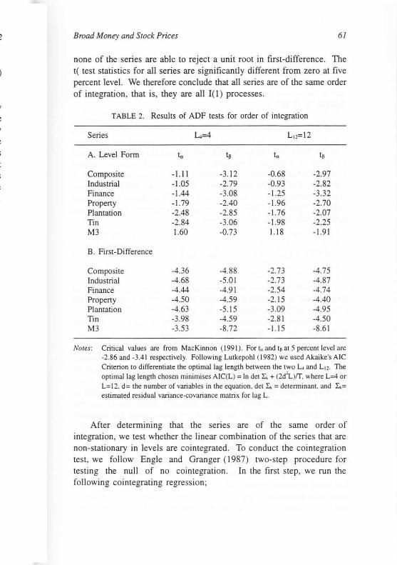
none of the series are able to reject a unit root in first-difference. The t( test statistics for all series are significantly different from zero at fi ve percent level. We therefore conclude that all series are of the same order of integration, that is, they are a1l 1(1) processes.
TABLE 2. Results of ADF tests for order of integration
Series
A. Level Form
Composite Industrial Finance Property Plantation Tin M3
B. First-Difference
Composite Industrial Finance Property Plantation Tin M3
1...=4
to
-1.11 -1.05 -1.44 -1.79 -2.48 -2.84 1.60
-4.36 -4.68 -4.44 -4.50 -4.63 -3.98 -3.53
L12=1 2
t, to
-3.12 -0.68 -2.79 -0.93 -3.08 -1.25 -2.40 -1.96 -2.85 -1.76 -3.06 -1.98 -0.73 1.1 8
-4.88 -2.73 -5.01 -2.73 -4.91 -2.54 -4.59 -2. 15 -5.15 -3.09 -4.59 -2.81 -8.72 -1.15
I,
-2.97 -2.82 -3.32 -2.70 -2.07 -2.25 -1.9 1
-4.75 -4.87 -4.74 -4.40 -4.95 -4.50 -8.6 1
Nores: Critical val ues are from MacK innon ( 199 1). For t" and Ip at 5 percen t level are -2.86 and -3.4 1 respective ly. Following LUlkepohl (1982) we used Akaike's Ale Criterion to differentiate the optimal lag length between the two L and L Ll. The optimal lag length chosen minimises AIC(L ) == In det r... + (2iL)ff. where L=4 or L== 12. d= the number of variables in the equat ion. det L. = determinant. and 4= estimated residual variance-covariance matrix for lag L.
After determining that the series are of the same order of integration, we test whether the linear combination of the series that are non-stationary in levels are coi ntegrated. To conduct the coi ntegration test, we follow Engle and Granger (1987) two-step procedure for test ing the null of no coi nlegration. In the first step, we run the foll owing cointegrating regression;

62 Jumai Ekonomi Malaysia 32
(II)
and in the second step, the ADF unit root test is conducted on the residual 11' as follows;
(12)
The null hypothesis is Ho: <p;O, that is S, and M, are not cointegrated by means of t-statistic of parameter <po The critical value is tabulated in MacKinnon (1991). If to is smaller than the critical value then S, and MI is said to be cointegrated. Apart from using the above residual-based tests for cointegrati on. we follow Engle and Granger (1987) in reporting the following cointegrating regression Durbin-Watson (CRDW) statistic computed as follow s;
( 13 )
The null hypothesis of no coi ntegration is rejected for value of CRDW which are significantly different from zero. The critical value for CRDW are tabulated in Engle and Yoo (1987).
The bivariate cointegration tests are presented in Table 3. For CRDW, in all cases, the null hypothesis of no co integration cannot be rejected. The calculated CRDW values are smaller than that of the critical value tabulated in Engle and Yoo ( 1987) at fi ve percent level of significance. Simi lar results can also be concluded from t ... test statistics. In all cases, the calculated trp test stat istics are larger than the critical value tabulated in MacKinnon (1991 ). Thus, the above results seem to suggest that broad money supply M3 and stock rrices in the Kuala Lumpur Stock Exchange are not cointegrated and therefore consistent with the efficient markets hypOlhesis. However. we subject the above analysis with further tests.

'2
e
j
j
Broad Money and Stock Prices 63
TABLE l. Results of cointegration rests
Cointegrating CRDW t.,.I-,=4 AIC t.,. L,,=12 AIC Regressions
Composi,e;f(M3) 0.14 -3.05 -5.01 -2.40 4.89 M3=f(Composi,e) 0.09 -2.60 -5.63 -1.97 -5.52
Industrial=f(M3) 0.13 -2.44 -5 .1 1 -2.1 9 -4.99 M3=f(lndustrial) 0.09 -1.93 -5.79 -1.68 -5.68
Finance=f(M3) 0.2 1 -2.94 -5.04 -2.84 -4.91 M3=f(Finance) 0.10 -2. 16 -5.24 -1.77 -5.10
Property=f(M3 ) 0.09 -2.23 -4.69 -2.47 -4.55 M3=f(Property) 0.02 -0.67 -6.30 -0.34 -6. 19
Pl an,a'ion=f(M3) 0.21 -2.69 -5.25 -1.94 -5.03 M3=f(Planta,ion) 0.01 -0.16 -6.50 0.20 -6.33
Tin=f(M3) 0.13 -2.97 -4.70 -2.12 -4.60 M3=f(Tin) 0.00 -0.02 -7.36 0.35 -7.28
Notes: Cri tical value for k. at 5 percent level is ·3.45 (see MacKinnon. 1991 ). Critical value: for CROW at 5 percent level is 0 .39 (see Engle and Yoo. 1987).
RESULTS WITH ERROR CORRECTION MODEL (ECM)
More recently, it has been recognised that the univariate analysis presented above has low power (for example, ADF and CROW) and have led Jenkinson ( 1986) and Banerjee e' a l. ( 1986) to recommend estimation of an Error Correction model as the starting point for mode lli ng and 'esting. Jenkinson ( 1986) po in' ed ou ' ,ha' 'he EngleGranger two-step estimation procedure is a form of static coinlcgrating regression in which the residual exhibit an autoregressive pattern. Furthennore. Sargan and Bhargava (1983) showed ,ha, 'he power of 'he CRDW test becomes very low as p approaches unity.2
Therefore. as an alternative lest for testing coi ntegration, the Error Correction Model (ECM) is 'he more appropria'e approach. The ECM
approach is derived from an important theorem presented by Engle and Granger ( 1987) ,ha' if a se' of va riables are coi n,egra,ed 'hen ,here
always exist an error correcting formulation of the dynamic mode l and

64 iumal Ekonomi Malaysia 32
vice versa. Using this approach, the residual from the cointegrating regression equation ( II ) are substituted into equations (5) and (6) and these equations are then re·estimated using OlS. Parameters 91 and e~ are then evaluated whether they are significantly different from zero. The significance of the error correction term (z\.a is sufficient enough (Q infer cointegration among the variables in question. Banerjee et al. (1986) have suggested that the ,-statistic of the error correction tenn as a more powerful statistic for testing the null of unit root. Furthermore, they also showed that under the alternative of cointegration this ,-statistic is more powerful than those of the Dickey-Fuller type tests.
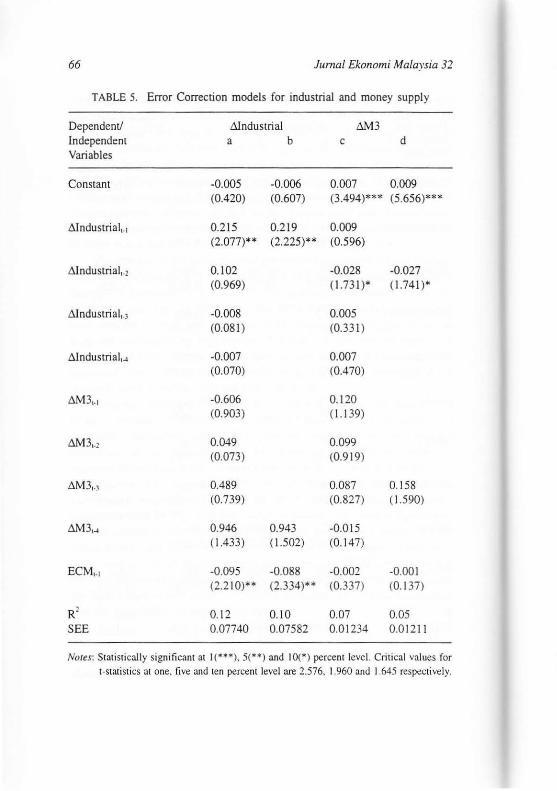
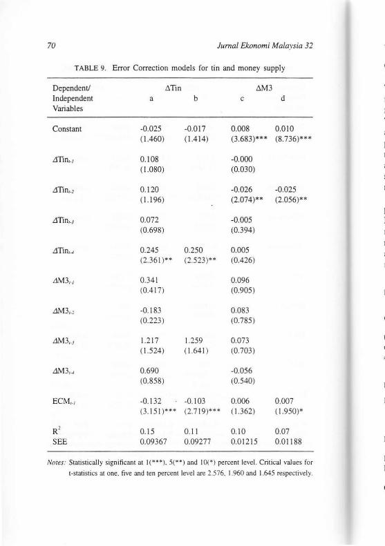
The results of the Error Correction models estimated for each of the stock price indexes and money supply M3 are presented in Tabl e 4 through 9 respectively for Composite , Industrial , Finance, Property, Plantation and Tin . In estimating the Error Correction regressions. we have selected K=N=4 and variables ECMt_1 represent the lagged residuals from the cointegrating regressions. For each series, we estimated the unrestricted Error Correction model s (a and c) with K=N=4, and the res tricted Error Correction models (b and d) after e liminating the insignificance variables but maintaining ECM t_j •
Looking through Tables 4 to 9, we can clearly see that (i) the ECM t_j variable is significantly different from zero in all regression equations es timated with stock price as dependent variable , but not otherwise; (ii) the effi ciency of the restricted Error Correction model imposed by excluding the insignificant variables is demonstrated by the decrease in the standard error of the regression (SEE) over the unrestricted regression; (iii) in all stoc k price equations, the error correction term ECM,_], has the correct negative sign and is significant , lending suppon to the finding that stock price and money supply M3 are coin tegrated, and in this case, money supply M3 Granger cause stock price; and (iv) in all money supply equations, the ECM,., variables has wrong positive sign and are not sign~ fi cantl y different from zero (except for Tin), which would imply an unstable dynamic adjustment mechanism and the possibility of omitted variables.
L
L
L
E
R S
N

2 Broad Money and Stock Prices 65
0 TABLE 4. Error Correction models for composite and money supply , j
.1Composite Dependent! t.M3 " Independent a b c d '. Variables J
Constant -0.016 -0.012 0.007 0.008 s ( 1.108) 0.2 16) (3.463)'" (5.597)'"
" : .1Composit~., 0.139 0.010
(1.380) (0707)
: 6Compositt;.2 0. 169 0. 168 -0.025 -0.024
1 ( 1.679)' 0.725)' (1.633) 0.624)
: .6.Composite,.) -0.0 15 -0.005 5 (0 143) (0.348) : , .6.Composite,-4 0.043 -0.003 , (0421) (0215)
DJv13,., -0.554 0.122 (0.797 (1. 144)
DJv13,.2 0.024 O.IM (0.034) (0.960)
1iM3!., 0.979 0.086 0.159 r ( 1.429) (08 15) (1.59 1)
llM3,.J 1.182 1.402 -0.024 ( 1.714)' (2. 127)" (0.231 )
ECM,., -0.140 -0. 128 0.001 0.001 (3.087)'" (3.050)'" (0.079) (0. 252)
R' 0. 16 0.12 0.07 0.05 SEE 0.07996 0.07929 0.0 1237 0.012 13
NOles: Statistically significant at 1(*"*),5(**) and 10(*) percent level. Critical values for l-sl::lIistics at one, five and len percent level are 2.576. 1.960 and 1.645 respectively.
66 lurnal Ekonomi Malaysia 32
TABLE 5. Error Correction models for industrial and money supply
Dependent! 6lndustrial 6M3 Independent a b c d Variables
Constant -0.005 -0.006 0.007 0.009 (0.420) (0.607) (3.494)*-- (5.656)***
.tiIndustrialt_1 0.215 0.219 0.009 (2.077)*- (2.225)*- (0.596)
.6.1ndustrial'.2 0.102 -0.028 -0.027
(0.969) (1.73 1)- (1.741)-
L\lndustrial {_ ~ -0.008 0.005 (0.081) (0.33 1 )
.6.lndustrial1-l -0.007 0.007 (0.070) (0.470)
.6.M3'_1 -0.606 0.120 (0.903) (1.139)
aM31_2 0.049 0.099 (0.073) (0.9 19)
.6.M31_) 0.489 0.087 0.158 (0 739) (0.827) ( 1.590)
aM31...! 0.946 0.943 -0.015 ( 1.433) ( 1.502) (0.147)
ECM,.J -0.095 -0.088 -0.002 -0.001 (2.2 10)'- (2.334)-' (0.337) (0.137)
R' 0.12 0.10 0.07 0.05 SEE 0.07740 0.07582 0.01234 0.01211
Noles: Statislically significant at 1( .... ).5(*"') and 10("') percent level. Critical values for I-Slalislics at one. five and ten percent level are 2.576. 1.960 and 1.645 respectively.

Broad Money and Stock Prices 67
TABLE 6. Error Correction models for finance and money supply
Dependent! 6Finance aM3 Independent a b c d Variables
Constant -0.10 -0.011 0.007 0.010 (0.754) (1.1 05) (3.458)"* (8.709)*"
dFinance,_1 0.106 0.012 (1.020) (0.780)
dFinance,_l 0.223 0.225 -0.030 -0.027 (2. 191 )** (2.323)" (2.047)** ( 1.879)*
dFinance,_3 -0.130 -0.009 (1212) (0.579)
dFinance,...,j 0.022 -0.001 (02 12) (0.112)
&vI3,_] -0.586 0.104 (0.828) (0.972)
LlM3,_2 0.210 0.106 (0.296) (0.974)
6M3,.; 0.398 0.084 (0.579) (0.798
&vI3,...,j 1.089 1.175 -0.017 ( 1.597) (1.815)* (0.168)
ECM'.I -0.155 -0. 161 0.005 0.008 (2.88 1 )"** (3.355)** * (0.854) ( 1.392)
R' 0.17 0.14 0.10 0.06 SEE 0.07982 0.07837 0.01215 0.01200
Notes: StJtislically sign ificanl at 1(*·*).5(**) and 10('") percent level. Crit ical values for t-slatislics at one. five and ten percent level are 2.576. 1.960 and 1.645 respectively

68 Jurnal Ekonomi Malaysia 32
TABLE 7. Error Correction models for property and money supply
Dependent! M'ropeny 6M3 Independent a b c d Variables
Constant -0.017 -0.014 0.007 0.10 ( 1.007) (!.I II ) (3.442)'" (8 .661 )'"
~PropenYl. 1 0.164 0.004 (1566) (0.309)
.6.PropertYl'! 0.250 0.270 -0.025 -0.024 (2.387)** (2.739)'" (1.911)' (1.990)"
M'ropertYl.3 -0.077 -0.004 (0.703) (0.314)
.6.PropertYl-' -0.006 -0.003 (0.058) (0.264)
8M3'.1 -0.601 0.102 (0.707) (0.945)
.6.M3,.! 0.208 0.096 (0.243) (0.884)
.6.M3,.~ 1.063 1.114 0.077 (1.297) ( 1.420) (0728)
.6.M 3'-i 0.818 -0.013 (0.992) (0.125)
ECM,., -0.082 -0.079 0.004 0.006 (2.255)** (2.392)**(0.847) (1373)
R' 0.15 0. 11 0.09 0.06 SEE 0.09518 0.09423 0.01221 0.01200
NOTes: Statistical ly significant a! 1('" **), 5(H ) and 10(*) percent level. Critical valut!s for 1-stati stics alone. five and ten percent level are 2.576. [.960 and 1.645 respectively.

2 Broad Money and Stock Prices 69
TABLE 8. Error Correction models for plantation and money supply
Dependent! 6.Plantation M13 Independent a b c d Variables
Constant -0.009 -0.0 14 0.008 0.009 (0.780) ( 1.582) (3.658)*** (5.6 13)***
LlPlantation,./ 0.144 0. 134 0.022 (1389) (1.364) ( 1.303)
LlPlantation,.] 0.0 18 -0.023 -0.019 (0. 180) ( 1.332) ( 1.1 51 )
LlPlantation/.J 0.023 0.000 (0.223) (0.024)
LlPlantation, ..... 0.065 -0.018 (0 .636) ( 1 048)
L1M3,./ -0.264 0.120 (0.436) (1.143)
<1."'13 ,., -0.607 0.057 (0.999) (0.545)
L1M3,_J 0.417 0.093 0.134 (0692) (0877) (1.3 15)
.&\113 , .... 1.198 1149 -0.062 (1991 )'* (2 .014)** (0592)
ECM,., -0.148 -0. 143 0.005 0.006 (2.702 )*** ( 2 .98 8 J ·~ ** (1223) (1443)
R' 0.14 0. 11 0.09 0.05 SEE 0.07037 0.06904 0.01220 0.01207
Note.f." Stati stically significant at 1("'*),5(") and 10(*) percent level. Crit ical val ues for
I-statistics at one , five and ten percent level are 2.576. 1.960 and 1.645 respectively.
70 JumaJ Ekonomi Malaysia 32
TABLE 9. Error Correction models for tin and money supply
Dependent! ~Tin aM3 Independent a b c d Variables
Constant -0.025 -0.017 0.008 0.010 ( 1.460) (1.414) (3.683)'" (8.736)'"
LiTin,., 0.108 -0.000 ( 1.080) (0.030)
.dlin'.l 0.120 -0.026 -0.025 (1. 196) (2.074)" (2.056)"
L1Tin,.J 0.072 -0.005 (0.698) (0394)
L1Tin,..,/ 0.245 0.250 0.005 (2.361 )*' (2.523)" (0.426)
L1M3 ,., 0.341 0.096 (0417 ) (0.905)
LiM3,.2 -0.183 0.083 (0.223) (0.785)
LiM3,.J 1.217 1.259 0.073 (1.524) (1.641 ) (0703) e
;
L1M3, . ..r 0.690 -0.056 (0.858) (0.540)
F
ECM,., -0.132 -0.103 0.006 0.007 E (3. 151 )*** (2.719)*** ( 1.362) ( 1.950)'
R' 0.15 0.11 0.10 0.07 SEE 0.09367 0.09277 0.01215 0.0 11 88 E
Notes: Statistically significant at 1(***). 5(H) and 10(*) percent level. Critical val ues for E
I-statistics at one. five and ten percenl level are 2.576. 1.960 and 1.645 respectivel y. E
C

Broad Money and SlOck Prices 7J
CONCLUSION
The present paper has applied recent developments in the theory of non-stationary regressors to analyse the empirical relationship between money supply M3 to stock prices in the Kuala Lumpur Stock Exchange. The results suggest that (i) all stock price indexes and money supply I are non-stationary in their level fonn , (ii) money supply M3 and stock prices are cointegrated suggesting the presence of an error-correction representation, relating the changes in the variables to lagged changes and a lagged combination of levels, and (iii) the error correction model suggest that M3 Granger cause stock prices, but not otherwise. These results is inconsistent with efficient markets hypothesis.
The above results suggest that to the viewpoint of the market participants, they will be able to predict stock prices in the Kuala Lumpur Stock Exchange using information on the growth of broad money supply M3 as the trading rule and can consistently earned excess returns. As to the monetary authority, broad money supply M3 can be a useful monetary instrument in affecting the stock market when the need arises.
NOTES
1The test stati st ics to and til are t-statistics of parameters ex and ~ in equations (7) and (9) respectivel y.
lFrom Table 3. we compute p using the expression CROW = 2 (l-p), and the first - order autoregressive coefficient is very close bUI not equal to one in each of the cointegrating regression. These values ranges from 0.90 for Finance
= f(M 3) to 0.99 for M3 = f (Tin).
REFERENCES
Banerjee, A .. J. J. DolJdo, D. F. Hendry & G.w. Smith. 1986. Exploring equilibrium re lati onships in econometric th rough static models: Some Monte Carlo Evidence. Oxford Bulletin of Economics and Statistics 48: 253-277.
Bank Negara Malaysia. 1990. Annual Report. Kuala Lumpur: Bank Negara Malaysia.
Bank Negara Malaysia. Quarterly Bulletin . Various issues. Box, G. E. P. & 1.M. Jenkins. 1970. Time Series Analysis Forecasting and
Control. San Francisco: HOlden-Day. Cooper, R. V L 1974. Efficient capital markets and [he quantity theory of Money.
)ourrla! of Fillanre 29: 88i -908.

72 Jllmal Ekonomi Malaysia 32
Dickey, D. A. & W. A. Fuller. 1979. Di stribution of the estimators for autoregressive time series with a unit root. Journal of American Statistical Association 74: 427A31.
Dickey, D.A. & W.A. Fuller. 1981. Likelihood ratio statistics for autoregressive time series with a unit root. Econometrica 49: 1057-1072.
Engle, R.F. & C.W.J. Granger. 1987. Coinregration and Error Correction: Representation, estimation and testing. Econometrica 55: 251-276.
Engle. R.F. & B. S. Yoo. 1987. Forecasting and testing in cointegrated systems. Journal of Econometrics 35: 143-159.
Ghosh. B.N. & S.c. Gan. 1994. On the choice of appropriate money stock fo r Malaysia. The Indian lournal of Economics 75(297): 269-278.
Granger, C.W.J. 1969. Investigating causal relations by econometric models and cross-spectral methods. Econometrica 37: 424.438.
Granger. C.W.J. 1981. Some properties of Time Series Data and their use in Econometric Model Specification. Journal of Econometrics 16: 121-130.
Granger, C.W.J. 1986. Developments in the study of Cointegrated Economic Variables. Oxford Bullet;1I of Economics and Statistics 48(3): 213-228.
Granger. C.W.J. 1988. Some Recnt Development in a Concept of Causality. Jotl11lal of Econometrics 36: 199-211.
Granger, c.W.J. & P. Newbold. 1977. Forecasting Economic Time Series. New York: Academic Press.
Gurley, J.G. & E.S. Shaw. 1960. MOlley if I the Theor), of Finance. Washingtong D.C.: The Brookings Institution.
Habibullah, M.S. 1992. Real Versus Nominal Adjustment Mechanism of the Malaysian Money Demand Function: Funher Evidence. Malaysian Management Journal 1(1): 57-69.
Hamburger, M.l & L.A. Kochin. 1972. Money and Swck Prices: The Channels of Influence. Journal of Finance 27: 231-249.
Ho, Y.K. 1983. Money Supply and Equity Prices: An Empirical Note on Far Eastern Countries. Economic Letters II : ! 61- 165.
Homa, K.E. & D.M . Jaffee . 1971. The Supply of Money and Common Stock Prices. Journal of Finance 26: 1056-1066.
leng. e.e.. l .S. BUller & l.T. Liu. 1990. The Informalional Efficiency of Ihe Stock Market: The International Evidence of 1921-1930. Economic LeIters 34: 157-162.
Jenkinson, T.J. 1986. Test ing Neo-Classical Theories of Labor Demand: An Application of Cointegration Techniques. Oxford Bulletin of Ecorzomics and Statistics 48(3): 24 1-251.
Jones, J.D. & N. Uri. 1987. Money Supply Growth, Stock Returns and the Direction of Causality. Socio -Economic Plallfling Science 21(5); 321-325.
Kraft. J. and A. Fraft. 1977a. Dete rminants of Common Stock Prices; A Time Series Analysis. Journal of Finance 32; 41 7-425.
Kraft , l & A. Kraft. 1977b. Common Stock Pri ces; Some Observations. Southern Economic JOllmal 43; 1365-1367.
Kuala Lumpur Stock Exchange. Investors Digest. Various issues.

Broad Money and Stock Prices 73
Lutkepohl, H. 1982. Non·Causality Due to Omitted Variables. lOl/mal of Econometrics 17: 367·378.
MacKinnon, 1. 1991. Critical Values for Cointegration Tests. In RF. Engle and CWJ. Granger (eds.). Long-Run Economic Relationships: Reading in Cointegration . New York: Oxford Uni versity Press.
Mookerjee, R. 1987. Monetary Policy and the Informational Efficiency of the Stock Market: The Evidence from Many Countries. Applied Economics 19: 1521-1532.
Muscatelli, V.A. 1991. Exogeneity, Cointegration and the Demand for Money in Italy. In T. Mayer and F. Spinelli (eds) . Macroeconomics and Macroeconomic Policy Issues. Aldershot: Avebury.
Nelson, C.R. & C.L Plosser. 1982. Trends and Random Walks in Macroeconomic Time Series. lournal of Moneta,..y Economics 10: 139·162.
Nowak, L.S. 1993 . Monetary Policy and Invesrmenr Opportunities. London: Quorum Books.
Rozeff, M.S. 1974. Money and Stock Prices. Journal of Financial Economics I: 245-302.
Sargan, J.D. & A. Bhargava. 1983. Testing Residuals from Least Squares Regres· sian for being generated by the Gaussian Random Walk. Econometrica 5 J :
153-174. Schwen, G.W. 1987. Effects of Model Specification as Tests for Unit Roots in
Macroeconomic Data. Journal of Monera,}' Economics 20: 73-103. Schwen, G.W. 1989. Tests for Unit Roots: A Monte Carlo Investigation.
Journal of Business alld ECOllOmic Statistics 7(2): 147-159. Sprinkel. B.W. 1964. MOlley and Stock Prices. Illinois: Richard D Irwin. Thornton, 1. 1993 . Mone y. Output and Stock Prices in the UK: Evidence on
Some (Non)relationships. Applied Financial Economics 3: 335-338.
Department of Economics Universiti Putra Malaysia 43400 UPM Serdang Selangor Darul Ehsan Malaysia