in silico alchemy - researchgate.net · abstract this tutorial explains how namd and related tools...

See discussions, stats, and author profiles for this publication at: https://www.researchgate.net/publication/265004753

In silico alchemy: A tutorial for alchemical free-energy perturbation

calculations with NAMD

Article

CITATIONS

2

4 authors, including:

Some of the authors of this publication are also working on these related projects:

Mitochondrial membrane fusion and membrane dynamics View project

Jérôme Hénin

French National Centre for Scientific Research

44 PUBLICATIONS 1,802 CITATIONS

SEE PROFILE

Chris Chipot

French National Centre for Scientific Research and University of Illin…

230 PUBLICATIONS 17,756 CITATIONS

SEE PROFILE

All content following this page was uploaded by Chris Chipot on 23 September 2015.

The user has requested enhancement of the downloaded file.

https://www.researchgate.net/publication/265004753_In_silico_alchemy_A_tutorial_for_alchemical_free-energy_perturbation_calculations_with_NAMD?enrichId=rgreq-0f0275eab8e3417847cc4af3c5581591-XXX&enrichSource=Y292ZXJQYWdlOzI2NTAwNDc1MztBUzoyNzY3NDk2MDM2MjI5MTNAMTQ0Mjk5MzY1NTQ0OA%3D%3D&el=1_x_2&_esc=publicationCoverPdf

https://www.researchgate.net/publication/265004753_In_silico_alchemy_A_tutorial_for_alchemical_free-energy_perturbation_calculations_with_NAMD?enrichId=rgreq-0f0275eab8e3417847cc4af3c5581591-XXX&enrichSource=Y292ZXJQYWdlOzI2NTAwNDc1MztBUzoyNzY3NDk2MDM2MjI5MTNAMTQ0Mjk5MzY1NTQ0OA%3D%3D&el=1_x_3&_esc=publicationCoverPdf

https://www.researchgate.net/project/Mitochondrial-membrane-fusion-and-membrane-dynamics?enrichId=rgreq-0f0275eab8e3417847cc4af3c5581591-XXX&enrichSource=Y292ZXJQYWdlOzI2NTAwNDc1MztBUzoyNzY3NDk2MDM2MjI5MTNAMTQ0Mjk5MzY1NTQ0OA%3D%3D&el=1_x_9&_esc=publicationCoverPdf

https://www.researchgate.net/?enrichId=rgreq-0f0275eab8e3417847cc4af3c5581591-XXX&enrichSource=Y292ZXJQYWdlOzI2NTAwNDc1MztBUzoyNzY3NDk2MDM2MjI5MTNAMTQ0Mjk5MzY1NTQ0OA%3D%3D&el=1_x_1&_esc=publicationCoverPdf

https://www.researchgate.net/profile/Jerome_Henin?enrichId=rgreq-0f0275eab8e3417847cc4af3c5581591-XXX&enrichSource=Y292ZXJQYWdlOzI2NTAwNDc1MztBUzoyNzY3NDk2MDM2MjI5MTNAMTQ0Mjk5MzY1NTQ0OA%3D%3D&el=1_x_4&_esc=publicationCoverPdf


https://www.researchgate.net/institution/French_National_Centre_for_Scientific_Research?enrichId=rgreq-0f0275eab8e3417847cc4af3c5581591-XXX&enrichSource=Y292ZXJQYWdlOzI2NTAwNDc1MztBUzoyNzY3NDk2MDM2MjI5MTNAMTQ0Mjk5MzY1NTQ0OA%3D%3D&el=1_x_6&_esc=publicationCoverPdf


https://www.researchgate.net/profile/Chris_Chipot?enrichId=rgreq-0f0275eab8e3417847cc4af3c5581591-XXX&enrichSource=Y292ZXJQYWdlOzI2NTAwNDc1MztBUzoyNzY3NDk2MDM2MjI5MTNAMTQ0Mjk5MzY1NTQ0OA%3D%3D&el=1_x_4&_esc=publicationCoverPdf




Nancy Universite, Universite Henri PoincareCentre National de la Recherche ScientifiqueEquipe de dynamique des assemblages membranaires,

Centre National de la Recherche ScientifiqueLaboratoire d’Ingenierie des Systemes Macromoleculaires

University of Illinois at Urbana-ChampaignBeckman Institute for Advanced Science and TechnologyTheoretical and Computational Biophysics Group

In silico alchemy: A tutorial for alchemical

free-energy perturbation calculations with NAMD

Jerome HeninJames Gumbart

Christopher HarrisonChristophe Chipot

January 31, 2012

Current editors: Chris Harrison ([email protected]) &Ivan Teo

Please visit www.ks.uiuc.edu/Training/Tutorials/ to get the latest version of this tutorial, to obtain

more tutorials like this one, or to join [email protected] mailing list for additional

help.

Abstract

This tutorial explains how NAMD and related tools can be used to setup and perform alchemical free-

energy simulations within the free-energy perturbation (FEP) theory. The force-field independent,

“zero-sum” transformation of ethane into ethane is used as an introductory, prototypical example.

FEP is then used to compute the free energy of charging a naked Lennard-Jones particle into a

sodium ion. Next, the variation in solvation free energy upon mutation of a tyrosine residue into

alanine is examined in the Ala–Tyr–Ala tripeptide. Last, the concept of standard binding free energy

is illustrated in the simple case of a potassium ion binding a ionophore, 18–crown–6. Prior knowledge

of NAMD and standard molecular dynamics simulations is assumed.

c© 2012, Centre National de la Recherche Scientifique, University of Illinois, Urbana–Champaign

2

Alchemical free-energy calculations tutorial 3

Contents

1. Ethane-to-ethane “zero-sum” transformation 5

1.1. System setup . . . . . . . . . . . . . . . . . . . . . . . . . . . . . . . . . . . . . . . . 5

1.2. Running the free energy calculation. . . . . . . . . . . . . . . . . . . . . . . . . . . . 8

1.3. Results. . . . . . . . . . . . . . . . . . . . . . . . . . . . . . . . . . . . . . . . . . . .10

1.4. Why a soft-core potential should always be included. . . . . . . . . . . . . . . . . . . 11

2. Charging a spherical ion 14

2.1. System setup . . . . . . . . . . . . . . . . . . . . . . . . . . . . . . . . . . . . . . . .14

2.2. Running the free energy calculation. . . . . . . . . . . . . . . . . . . . . . . . . . . . 15

2.3. Results. . . . . . . . . . . . . . . . . . . . . . . . . . . . . . . . . . . . . . . . . . . .17

3. Mutation of tyrosine into alanine 20

3.1. System setup . . . . . . . . . . . . . . . . . . . . . . . . . . . . . . . . . . . . . . . .20

3.2. Running the free energy calculations. . . . . . . . . . . . . . . . . . . . . . . . . . . . 24

3.3. Results. . . . . . . . . . . . . . . . . . . . . . . . . . . . . . . . . . . . . . . . . . . .26

4. Binding of a potassium ion to 18–crown–6 29

4.1. System setup . . . . . . . . . . . . . . . . . . . . . . . . . . . . . . . . . . . . . . . .30

4.2. Running the free energy calculations. . . . . . . . . . . . . . . . . . . . . . . . . . . . 32

4.3. Results. . . . . . . . . . . . . . . . . . . . . . . . . . . . . . . . . . . . . . . . . . . .35


Introduction

The goal of this tutorial is to guide the user in setting up free energy calculations of alchemical trans-

formations [1] within NAMD. [ 2, 3] We will first perform the rather simple, “zero-sum” transformation

of ethane into ethane in water. In a second case example, we calculate the free energy of charging a

naked Lennard-Jones sphere into a sodium ion, recovering in a computer simulation a result predicted

over eighty years ago by the Born model. [4] Last, as a more practical example, we will compute the

difference in hydration free energy resulting from the mutation of tyrosine into alanine in the Ala–Tyr–

Ala tripeptide. As has been commented on amply, suchin silico experiments have not reached yet the

maturity to be viewed as black-box, routine jobs, [5, 6, 7] which implies that both the sampling strategy

and the analysis of the results should be considered with great care.

NAMD makes use of the so-calleddual topologyapproach, [8, 9] in which both the initial state,viz.λ =

0, and the final state,viz.λ = 1, are defined concurrently. As the molecular dynamics (MD) simulation

progresses, the potential energy function characteristic ofλ = 0 is scaled into that representative ofλ = 1.

Whereas the initial and the final states do interact with the environment, we typically do not allow them

to see each other in the course of the+ transformation. For versions of NAMD prior to 2.7b2, achieving

these conditions requires that a list of excluded atoms be defined in the PSF topology file. Since the

psfgen software supplied with NAMD does not offer a way of building such a list, we provide the

alchemify program.alchemify processes PSF files written bypsfgen or CHARMM and makes

them suitable for simulating alchemical transformations. However, in NAMD 2.7b2, the appropriate

exclusions are generated automatically at the start of the simulations.

The reader of this tutorial is assumed to be familiar with the use of NAMD to perform “standard” cal-

culations, including energy minimization and MD simulations. General documentation, tutorials and

templates of NAMD configuration files are available from the Documentation section of the NAMD web

page. The simulation times in this tutorial are very short in the interest of expediency; however, one

should be aware that they are generally insufficient for most applications. Additionally, although not

always used in the tutorial, equilibration of a system prior to running FEP simulations is highly recom-

mended.

Completion of this tutorial requires:

• various files contained in the archiveFEP tutorial.zip , provided with this document;


• NAMD 2.7b2 [3] or later (http://ks.uiuc.edu/Research/namd );

• VMD 1.8.4 [10] or later (http://ks.uiuc.edu/Research/vmd );

• alchemify (only needed for versions of NAMD before 2.7b2

http://www.edam.uhp-nancy.fr/Alchemify ).

1. Ethane-to-ethane “zero-sum” transformation

Perhaps the simplest alchemical transformation one could imagine, the result of which is completely

independent of the potential energy function utilized, is thezero-sumethane→ ethane mutation, [11, 9]

wherein a methyl group vanishes at one end of the molecule, while another one appears at the other end.

The accuracy of the computed free energy only depends on the sampling strategy adopted, regardless of

the force field employed.

1.1. System setup

To set up a system, you will need a structure file (PSF) and a coordinate file (PDB). We have provided

you with the coordinate files for both ethane and water, as well as the topology files needed to build the

structure files. In addition, FEP calculations in NAMD require thealchFile which will be introduced

to you in greater detail later.

H

HH

H

commonpart

C

H

C

C

H HH

H H

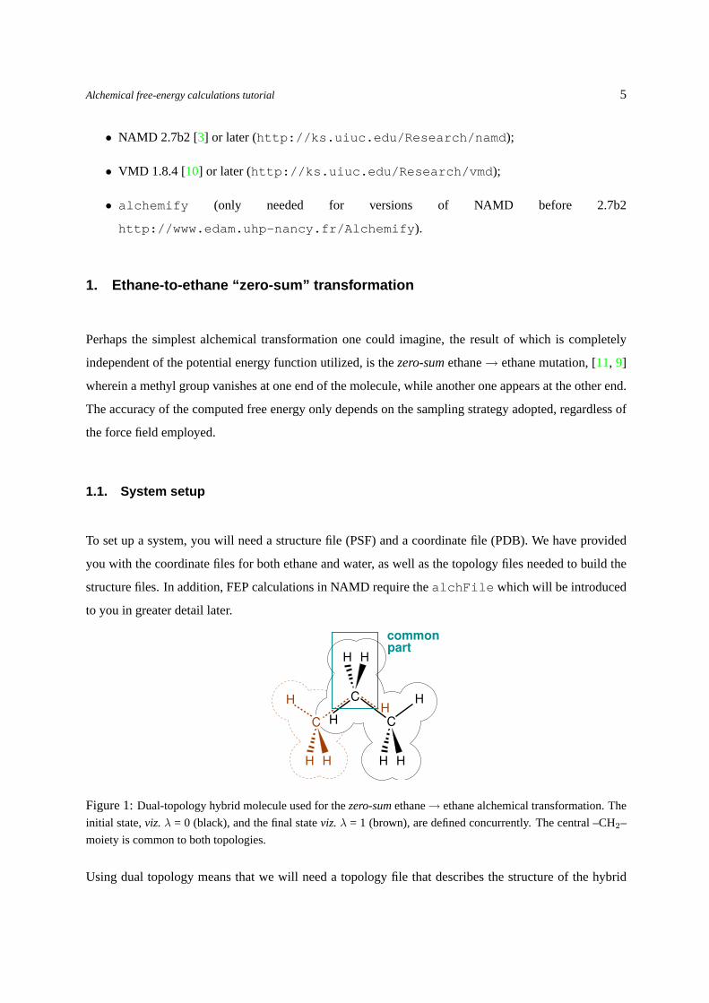
Figure 1:Dual-topology hybrid molecule used for thezero-sumethane→ ethane alchemical transformation. The

initial state,viz.λ = 0 (black), and the final stateviz.λ = 1 (brown), are defined concurrently. The central –CH2–

moiety is common to both topologies.

Using dual topology means that we will need a topology file that describes the structure of the hybrid


molecule. Although such a file,zero.top , has been provided for you in this case, the hybrid topology

file is in general created by the user.

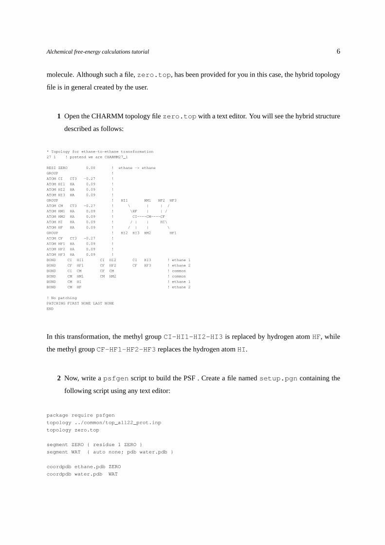
1 Open the CHARMM topology filezero.top with a text editor. You will see the hybrid structure

described as follows:

* Topology for ethane-to-ethane transformation

27 1 ! pretend we are CHARMM27_1

RESI ZERO 0.00 ! ethane -> ethane

GROUP !

ATOM CI CT3 -0.27 !

ATOM HI1 HA 0.09 !

ATOM HI2 HA 0.09 !

ATOM HI3 HA 0.09 !

GROUP ! HI1 HM1 HF2 HF3

ATOM CM CT3 -0.27 ! \ | | /

ATOM HM1 HA 0.09 ! \HF | | /

ATOM HM2 HA 0.09 ! CI----CM----CF

ATOM HI HA 0.09 ! / | | HI\

ATOM HF HA 0.09 ! / | | \

GROUP ! HI2 HI3 HM2 HF1

ATOM CF CT3 -0.27 !

ATOM HF1 HA 0.09 !

ATOM HF2 HA 0.09 !

ATOM HF3 HA 0.09 !

BOND CI HI1 CI HI2 CI HI3 ! ethane 1

BOND CF HF1 CF HF2 CF HF3 ! ethane 2

BOND CI CM CF CM ! common

BOND CM HM1 CM HM2 ! common

BOND CM HI ! ethane 1

BOND CM HF ! ethane 2

! No patching

PATCHING FIRST NONE LAST NONE

END

In this transformation, the methyl groupCI-HI1-HI2-HI3 is replaced by hydrogen atomHF, while

the methyl groupCF-HF1-HF2-HF3 replaces the hydrogen atomHI .

2 Now, write apsfgen script to build the PSF . Create a file namedsetup.pgn containing the

following script using any text editor:

package require psfgen

topology ../common/top_all22_prot.inp

topology zero.top

segment ZERO { residue 1 ZERO }

segment WAT { auto none; pdb water.pdb }

coordpdb ethane.pdb ZERO

coordpdb water.pdb WAT


writepsf setup.psf

writepdb setup.pdb

The script you have entered tellspsfgen to generate a system consisting of the hybrid molecule and

water (PDB provided), using structural information from the named topology files.

3 In the VMD TkConsole, run the script usingsource setup.pgn . You have now created a

PDB and a PSF file,setup.pdb andsetup.psf . An example output has been provided in the

example-output folder.

In the next step, you will create thealchFile . Recall that the system you have created contains a)

atoms in the initial state that will gradually vanish, b) atoms that will gradually appear towards the final

state, and c) atoms that are present throughout the whole transformation. NAMD distinguishes between

these three classes of atoms based on information in thealchFile . The alchFile is essentially

the PDB file of your system, except that every atom has been tagged according to the class to which it

belongs.

4 Opensetup.pdb in a text editor. Change the B column so that vanishing and appearing atoms

are tagged with a -1.00 and 1.00 flag respectively, while unchanging atoms are tagged with 0.00.

The required changes are shown below:

ATOM 1 CI ZERO 1 -1.167 0.224 0.034 1.00 -1.00 ZERO

ATOM 2 HI1 ZERO 1 -2.133 -0.414 0.000 1.00 -1.00 ZERO

ATOM 3 HI2 ZERO 1 -1.260 0.824 0.876 1.00 -1.00 ZERO

ATOM 4 HI3 ZERO 1 -1.258 0.825 -0.874 1.00 -1.00 ZERO

ATOM 5 CM ZERO 1 0.001 -0.652 -0.002 1.00 0.00 ZERO

ATOM 6 HM1 ZERO 1 0.000 -1.313 -0.890 1.00 0.00 ZERO

ATOM 7 HM2 ZERO 1 0.005 -1.308 0.889 1.00 0.00 ZERO

ATOM 8 HI ZERO 1 1.234 0.192 0.000 1.00 -1.00 ZERO

ATOM 9 HF ZERO 1 -1.237 0.190 0.000 1.00 1.00 ZERO

ATOM 10 CF ZERO 1 1.289 0.150 -0.078 1.00 1.00 ZERO

ATOM 11 HF1 ZERO 1 2.149 -0.425 -0.001 1.00 1.00 ZERO

ATOM 12 HF2 ZERO 1 1.256 0.837 -0.893 1.00 1.00 ZERO

ATOM 13 HF3 ZERO 1 1.131 0.871 0.940 1.00 1.00 ZERO

ATOM 14 OH2 TIP3 1 -5.574 -5.971 -9.203 1.00 0.00 WAT

ATOM 15 H1 TIP3 1 -5.545 -5.020 -9.301 1.00 0.00 WAT

...

5 Once you have made the necessary changes, save the file aszero.fep .

You may find it helpful at this stage to visualize the system with its initial and final groups. Doing so

makes it easy to spot errors made in the previous steps.


6 Run VMD with the following command:vmd setup.psf -pdb zero.fep .

7 In the Graphics/Representations menu, set the selection text to “not water” and select the coloring

methodBeta . Appearing atoms are colored blue and vanishing atoms are colored red, while the

unperturbed part of the molecule appears in green. Compare the result with Figure1. Can you see

clearly which atoms will vanish and which will appear?

8 If you are using NAMD 2.7b2 or later, you can skip this step. Callalchemify using the follow-

ing command line:

alchemify setup.psf zero.psf zero.fep

In the system we have defined, appearing and vanishing atoms interact in two ways: through non–bonded

forces, and because some of the angle and dihedral parameters automatically generated bypsfgen cou-

ple the two end-points of the transformation. For instance, theCI-CM-CF angle should not be assigned

a force field term by NAMD. To prevent unwanted non–bonded interactions,alchemify processes

PSF files and creates the appropriate non–bonded exclusion list. At the same time, irrelevant bonded

terms that involve appearing and vanishing atoms are removed.alchemify retrieves the necessary

data about the transformation fromalchFile . These unwanted terms are automatically ignored in

NAMD versions 2.7b2 and later.

If you have calledalchemify the resulting filezero.psf will be used when performing the FEP

calculations.

1.2. Running the free energy calculation

1 Open with a text editor the provided configuration files for the forward and backward transforma-

tions,forward-noshift.namd andbackward-noshift.namd respectively.

You can tell from the configuration files that we will be doing an MD run at a constant temperature of

300 K and pressure of 1 bar, using particle-mesh Ewald (PME) electrostatics. Furthermore, we have

set therigidBonds option toall and the time step to 2 fs. To impose isotropic fluctuations of the

periodic box dimensions, we set theflexibleCell variable tono . We define the initial periodic box


to be a cube with an edge length of 21.8A. The simulation takes as its input the output files (provided)

of an equilibration run, so there is no need to run an equilibration in this example.

Take a look at the FEP section of the configuration file. This section defines the sampling strategy of

the calculation. This section calls a TCL script fep.tcl that defines three commands to simplify the

syntax of FEP scripts:

• runFEP runs a series of FEP windows between equally-spacedλ-points, whereas

• runFEPlist uses an arbitrary, user-supplied list ofλ values.

• runFEPmin is identical to runFEP but adds an initial minimization step as well (use this only for

equilibration runs).

The FEP section of the configuration file for the forward transformation reads:

# FEP PARAMETERS

source ../tools/fep.tcl

alch on

alchType FEP

alchFile zero.fep

alchCol B

alchOutFile forward-noshift.fepout

alchOutFreq 10

alchVdwLambdaEnd 1.0

alchElecLambdaStart 1.0

alchVdWShiftCoeff 0.0

alchDecouple no

alchEquilSteps 100

set numSteps 500

runFEP 0.0 1.0 0.0625 $numSteps

In the above example, the potential energy function of the system is scaled fromλ = 0 toλ = 1 by incre-

mentsδλ = 0.0625,i.e.16 intermediateλ-states or “windows”. [7] In each window, the system is equili-

brated overalchEquilSteps MD steps, here 100 steps, prior to$numSteps - alchEquilSteps

= 400 steps of data collection, from which the ensemble average is evaluated. As you can see from the

script, there are other FEP variables defined in this section that we have not mentioned. These variables

correspond to the soft-core potential and will be introduced to you later.


2 Run the forward and backward simulations by entering the commands

namd2 forward-noshift.namd > forward-noshift.log

namd2 backward-noshift.namd > backward-noshift.log

in a terminal window. Each simulation should require only a few minutes.

1.3. Results

Figure 2: Free-energy change for the ethane→ ethanezero-summutation, measured in the forward and in the

backward direction. This simulation was performed in the absence of a soft-core potential. [12, 13] Singularities

are manifested at the end points, whenλ = 0 or 1.

The alchOutFile contains all data resulting from the FEP calculation. In order to obtain the∆G

profile shown above, we will have to extract only the relevant portions and parse it into a format amenable

to graph plotting.

1 If you are on a UNIX or Macintosh system, extract the∆G(λ) profile using this command line:

grep change forward-noshift.fepout | awk ’ {print $9, $19 }’ >

forward-noshift.dat

Alternatively, you can use the provided scriptdeltaA.awk in thetools directory, i.e.,

../tools/deltaA.awk forward-noshift.fepout > forward-noshift.dat

This creates a two-column data file that can be read by most plotting programs,e.g.xmgrace, gnuplot, or


any spreadsheet application.

An example of the expected result is plotted in Figure2. One of the notorious shortcomings of the dual-

topology paradigm can be observed in the∆G(λ) profile whenλ approaches 0 or 1. In these regions,

interaction of the reference or the target topology with its environment is minute, yet strictly nonzero.

Molecules of the surroundings can in turn clash against incoming or outgoing chemical moieties, which

can lead to numerical instabilities in the trajectory, manifested in large fluctuations in the average poten-

tial energy. The result is slow convergence. [7]

There are two ways we can go about handling these so-called “end-point catastrophes”. One is to em-

ploy a better-adapted sampling strategy. The other is to use a soft-core potential, [12, 13, 14] which

effectively eliminates the singularities atλ = 0 or 1, by progressively decoupling interactions of outgoing

atoms and coupling interactions of incoming atoms. This feature is available by default in NAMD. For

pedagogical purposes, however, the parameters that control the soft-core potential in the example you

have just done —viz. alchVdwLambdaEnd , alchElecLambdaStart , alchVdWShiftCoeff

andalchDecouple , were not set to apply a correction.

Having seen the deleterious effects of possible end-point singularities, we will now use a soft-core po-

tential to prevent such singularities from occuring.

1.4. Why a soft-core potential should always be included

We will now run the FEP calculation again, but using this time a soft-core potential, hence avoiding the

need for narrower windows asλ gets closer to 0 or 1.

1 Openforward-shift.namd in a text editor.

Note that the configuration script differs fromforward-noshift.namd in only the FEP section,

which is as follows:

# FEP PARAMETERS



alch on

alchType FEP

alchFile zero.fep

alchCol B

alchOutFile forward-shift.fepout

alchOutFreq 10




alchDecouple yes

alchEquilSteps 100

set numSteps 500


The parameters utilized for the soft-core potential are rather detailed and can be somewhat confusing, so

be sure to read the following carefully. Outgoing atoms will see their electrostatic interactions with the

environment decoupled duringλ = 0 to 1− alchElecLambdaStart = 0.5, while the interactions

involving incoming atoms are progressively coupled duringλ = 1− alchElecLambdaStart to 1.

At the same time, van der Waals interactions involving vanishing atoms are progressively decoupled

duringλ = 1− alchVdwLambdaEnd , i.e. 0 to 1, while the interactions of appearing atoms with the

environment become coupled duringλ = 1 to 1− alchVdwLambdaEnd , i.e.0.

2 Run the new forward and backward simulations using the commands

namd2 forward-shift.namd > forward-shift.log

namd2 backward-shift.namd > backward-shift.log

in a terminal window and analyze the resulting output.

Figure3 shows a typical result for this new simulation. The effect of the soft-core potential is apparent

in the total free energy change, now close to zero, and the symmetry of the profile with respect toλ

= 0.5, which altogether suggests that the calculation has converged. However, greater sampling will

improve convergence further. If desired, try running the simulationforward-shift-long.namd ,

which multiplies the length by a factor of 10, to see if it improves the result (NOTE: this simulation may

take 30 minutes or more!).


Figure 3:Result of an ethane→ ethanezero-summutation including a soft-core potential correction to circumvent

the “end-point catastrophes” highlighted in Figure2. Using an equally modest sampling strategy, the expected

zero free-energy change is recovered. Note the overlapping profiles obtained from the forward and the backward

transformations.

Probing the convergence properties of the simulation

We can assess convergence of the free energy calculation by monitoring the time-evolution

of ∆G(λ) for every individualλ-state and the overlap of configurational ensembles embod-

ied in their density of states,P0[∆U(x)] andP1[∆U(x)], where∆U(x) = U1(x)−U0(x)denotes the difference in the potential energy between the target and the reference states.

Since a soft-core potential [12, 13] has been introduced to avoid the so-called “end-point

catastrophes”, the potential energy no longer varies linearly with the coupling parameterλ.

Therefore, it is necessary that the reverse transformation be carried out explicitly to access

∆Gλ+δλ→λ, as is proposed in the above NAMD scripts.


2. Charging a spherical ion

In the second example of this tutorial, we will charge a naked Lennard-Jones particle into a sodium ion

in an aqueous environment.

2.1. System setup

Our system consists of a sodium ion immersed in a bath of water molecules. Using the dual-topology

paradigm, we could charge a Lennard-Jones particle by shrinking a naked spherical particle, while grow-

ing concomitantly the ion. However, in this particular example, the single-topology approach would

have the benefit of perturbing only the electrostatic component of the nonbonded potential, thus avoiding

perturbing the Lennard-Jones terms and improving convergence. We can emulate such a single-topology

paradigm within the dual-topology approach implemented in NAMD, simply by choosing appropriate

parameters for the soft-core potential and the coupling of the particle with its environment.

1 Generate the PSF and PDB files for the system, which is a sodium ionSODat the center of a water

box. You can do this by creating a file namedsetup.pgn containing the script below. Run the

script you have written by going to the VMD TkConsole and enteringsource setup.pgn .


segment SOD {

residue 1 SOD

}

writepsf setup.psf

writepdb setup.pdb

2 Next, you will surround the ion with a water box using theSolvate plugin of VMD. Call the

Solvate plugin in the TkConsole with the following:solvate setup.psf setup.pdb

-t 15 -o solvate

We want the primary cell be large enough to minimize the self-interaction of the cation between adjacent

boxes. For this purpose, a box length of 30Awill do. The distance separating the cation in the primary


and the adjacent cells being equal to 30A, the interaction energy reduces toq2/4πε0ε1r = 0.1 kcal/mol

with an ideal macroscopic permittivity of 78.4 for bulk water.

3 Unlike the previous example, the system has not been pre-equilibrated for you. Conduct an equili-

bration run using the provided configuration fileequilibration.namd by entering the com-

mand

namd2 equilibration.namd > equilibration.log

in a terminal window.

4 You are now ready to run the FEP calculation. As before, you must build thealchFile by

editing the B column of the PDB file to indicate which atoms are appearing and disappearing.

Open with a text editor thesolvate.pdb file generated by theSolvate plugin.

5 Edit the relevant line to reflect the growing sodium ion, then save the file assolvate.fep .

ATOM 1 SOD SOD 1 0.000 0.000 0.000 1.00 1.00 SOD

...

6 In the present system, sinceSODdoes not coexist with any other perturbed particle, you do not

have to usealchemify to remove extra terms in the PSF file.

7 As a safety check, you should consider both forward,i.e.charge creation, and backward,i.e.charge

annihilation, transformations. Repeat the procedure described in this section for the backward

calculation.

2.2. Running the free energy calculation

The NAMD implementation of the soft-core potential [12] allows us to decouple at a different pace the

van der Waals and the electrostatic interactions of the perturbed system with its environment, as depicted

in Figure4. In our current case, we can independently modify each of the forces so that the Lennard-

Jones coupling remains the same throughout (the neutral particle never disappears) while electrostatic

interactions are scaled up or down.


Figure 4: Decoupling of electrostatic and van der Waals interactions within the NAMD implementation of

the soft-core potential. Solid lines represent outgoing atoms and dashed lines represent incoming atoms.

Two variables define how the perturbed system is coupled or decoupled from its environment,viz. λelec

(alchElecLambdaStart ) andλvdW (alchVdwLambdaEnd ). In the present scenario,λvdW = 1.0, meaning

that the van der Waals interactions for outgoing and incoming particles will be, respectively, scaled down starting

from λ = 1.0 − λvdW = 0.0 to λ = 1.0, and scaled up starting fromλ = 0.0 to λ = λvdW. If λelec = 0.4,

electrostatic interactions for outgoing and incoming particles are, respectively, scaled down from 0.0 to 1.0 -λelec

= 0.6, and scaled up fromλelec to 1.0.

By setting bothalchElecLambdaStart andalchVdwLambdaEnd to 0.0, we begin scaling down

electrostatic interactions of the vanishing atoms atλ = 0.0, until the interactions completely disappear at

λ = 1.0, and for appearing atoms, scaling up fromλ = 0.0 toλ = 1.0, while van der Waals interactions

remain unchanged.

You can set the above parameters in the FEP section of the NAMD configuration file. Take a look, for

example, atforward.namd :

# FEP PARAMETERS


alch on

alchType FEP

alchFile solvate.fep

alchCol B

alchOutFile forward.fepout

alchOutFreq 10




alchDecouple on


alchEquilSteps 100

set numSteps 500


The sampling strategy we will use involves 16 equally spaced windows withδλ = 0.0625. Each window

features 500 steps of MD sampling, among which 100 steps are equilibration. Assuming a time step of

2 fs for integrating the equations of motion, the total simulation time amounts to 16 ps. We will find that

this time scale is appropriate for reproducing the expected charging free energy.

In the traditional MD section, we use standard NAMD configuration parameters. Langevin dynamics is

employed to maintain constant temperature at 300 K. The Langevin piston enforces a constant pressure of

1 bar. Long-range electrostatic forces are handled by means of the PME algorithms. All chemical bonds

are frozen to their equilibrium value and a time step of 2 fs is used. To impose isotropic fluctuations

of the periodic box dimensions,flexibleCell has been set tono . The initial periodic cell, prior to

equilibration, is defined as a cube with an edge length of 30.0A.

1 Before performing the FEP calculations, you will first need to equilibrate the system. Run an

equilibration usingnamd2 equilibration.namd > equilibration.log .

2 Run both the forward and backward simulations using the commands

namd2 forward.namd > forward.log

namd2 backward.namd > backward.log

in a terminal window.

2.3. Results

The free energy profile delineating the alchemical transformation is shown in Figure5.

1 Obtain this profile by using again thegrep command on thealchOutFile , as you did in the

first example of this tutorial.


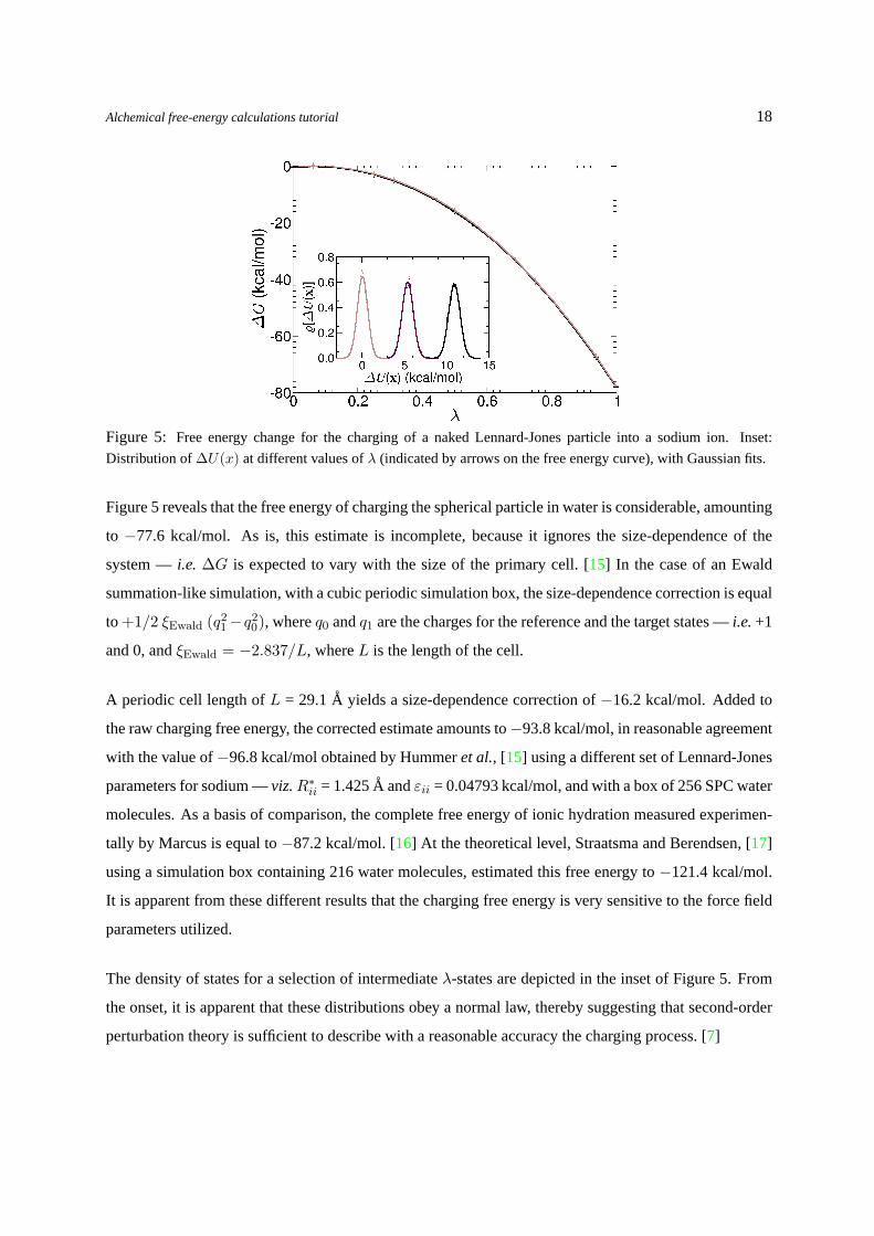
Figure 5: Free energy change for the charging of a naked Lennard-Jones particle into a sodium ion. Inset:

Distribution of∆U(x) at different values ofλ (indicated by arrows on the free energy curve), with Gaussian fits.

Figure5 reveals that the free energy of charging the spherical particle in water is considerable, amounting

to −77.6 kcal/mol. As is, this estimate is incomplete, because it ignores the size-dependence of the

system —i.e. ∆G is expected to vary with the size of the primary cell. [15] In the case of an Ewald

summation-like simulation, with a cubic periodic simulation box, the size-dependence correction is equal

to +1/2 ξEwald (q21−q2

0), whereq0 andq1 are the charges for the reference and the target states —i.e.+1

and 0, andξEwald = −2.837/L, whereL is the length of the cell.

A periodic cell length ofL = 29.1A yields a size-dependence correction of−16.2 kcal/mol. Added to

the raw charging free energy, the corrected estimate amounts to−93.8 kcal/mol, in reasonable agreement

with the value of−96.8 kcal/mol obtained by Hummeret al., [15] using a different set of Lennard-Jones

parameters for sodium —viz.R∗ii = 1.425A andεii = 0.04793 kcal/mol, and with a box of 256 SPC water

molecules. As a basis of comparison, the complete free energy of ionic hydration measured experimen-

tally by Marcus is equal to−87.2 kcal/mol. [16] At the theoretical level, Straatsma and Berendsen, [17]

using a simulation box containing 216 water molecules, estimated this free energy to−121.4 kcal/mol.

It is apparent from these different results that the charging free energy is very sensitive to the force field

parameters utilized.

The density of states for a selection of intermediateλ-states are depicted in the inset of Figure5. From

the onset, it is apparent that these distributions obey a normal law, thereby suggesting that second-order

perturbation theory is sufficient to describe with a reasonable accuracy the charging process. [7]


Improving the agreement with experiment

Replacing the standard CHARMM Lennard-Jones parameters for sodium by those chosen

by Hummeret al., [15] verify that the charging free energy coincides with the estimate

reached by these authors.

Recovering predictions from the Born model

Granted that water is a homogeneous dipolar environment, the charging free energy writes

∆G = −β/2 q2 〈V 2〉0, whereV is the electrostatic potential created by the solvent on the

charge,q. Increasingq to +2, show that the charging free energy varies quadratically with

the charge, as predicted by the Born model —i.e.∆G = (ε− 1)/ε× q2/2a, wherea is the

radius of the spherical particle andε, the macroscopic permittivity of the environment.


3. Mutation of tyrosine into alanine

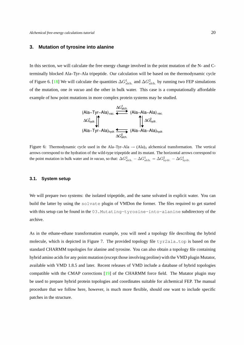
In this section, we will calculate the free energy change involved in the point mutation of the N- and C-

terminally blocked Ala–Tyr–Ala tripeptide. Our calculation will be based on the thermodynamic cycle

of Figure6. [18] We will calculate the quantities∆G1alch. and∆G2

alch. by running two FEP simulations

of the mutation, onein vacuoand the other in bulk water. This case is a computationally affordable

example of how point mutations in more complex protein systems may be studied.

hydr.∆G1

hydr.∆G2

alch.∆G2

alch.∆G1

(Ala−Ala−Ala)

(Ala−Ala−Ala)

vac.

hydr.

vac.

hydr.(Ala−Tyr−Ala)

(Ala−Tyr−Ala)

Figure 6: Thermodynamic cycle used in the Ala–Tyr–Ala→ (Ala)3 alchemical transformation. The vertical

arrows correspond to the hydration of the wild-type tripeptide and its mutant. The horizontal arrows correspond to

the point mutation in bulk water andin vacuo, so that:∆G2alch. −∆G1

alch. = ∆G2hydr. −∆G1

hydr.

3.1. System setup

We will prepare two systems: the isolated tripeptide, and the same solvated in explicit water. You can

build the latter by using thesolvate plugin of VMDon the former. The files required to get started

with this setup can be found in the03.Mutating-tyrosine-into-alanine subdirectory of the

archive.

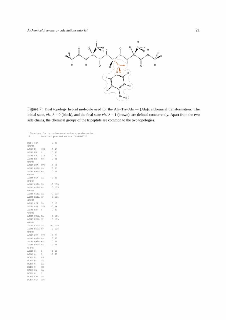
As in the ethane-ethane transformation example, you will need a topology file describing the hybrid

molecule, which is depicted in Figure7. The provided topology filetyr2ala.top is based on the

standard CHARMM topologies for alanine and tyrosine. You can also obtain a topology file containing

hybrid amino acids for any point mutation (except those involving proline) with the VMD plugin Mutator,

available with VMD 1.8.5 and later. Recent releases of VMD include a database of hybrid topologies

compatible with the CMAP corrections [19] of the CHARMM force field. The Mutator plugin may

be used to prepare hybrid protein topologies and coordinates suitable for alchemical FEP. The manual

procedure that we follow here, however, is much more flexible, should one want to include specific

patches in the structure.


H

CH

H

H

C

H

C

HH

H

H H

H

H C H

C

H

H

OH

HC

CC

C

H

O

O

N

H O

CHCC

C N

H

C NC

O

N C

H

H C HH

H

H

C

H

Figure 7: Dual topology hybrid molecule used for the Ala–Tyr–Ala→ (Ala)3 alchemical transformation. The

initial state,viz.λ = 0 (black), and the final stateviz.λ = 1 (brown), are defined concurrently. Apart from the two

side chains, the chemical groups of the tripeptide are common to the two topologies.

* Topology for tyrosine-to-alanine transformation

27 1 ! Version: pretend we are CHARMM27b1

RESI Y2A 0.00

GROUP

ATOM N NH1 -0.47

ATOM HN H 0.31

ATOM CA CT1 0.07

ATOM HA HB 0.09

GROUP

ATOM CBA CT2 -0.18

ATOM HB1A HA 0.09

ATOM HB2A HA 0.09

GROUP

ATOM CGA CA 0.00

GROUP

ATOM CD1A CA -0.115

ATOM HD1A HP 0.115

GROUP

ATOM CE1A CA -0.115

ATOM HE1A HP 0.115

GROUP

ATOM CZA CA 0.11

ATOM OHA OH1 -0.54

ATOM HHA H 0.43

GROUP

ATOM CD2A CA -0.115

ATOM HD2A HP 0.115

GROUP

ATOM CE2A CA -0.115

ATOM HE2A HP 0.115

GROUP

ATOM CBB CT3 -0.27

ATOM HB1B HA 0.09

ATOM HB2B HA 0.09

ATOM HB3B HA 0.09

GROUP

ATOM C C 0.51

ATOM O O -0.51

BOND N HN

BOND N CA

BOND C CA

BOND C +N

BOND CA HA

BOND O C

BOND CBA CA

BOND CGA CBA


BOND CD2A CGA

BOND CE1A CD1A

BOND CZA CE2A

BOND OHA CZA

BOND CBA HB1A

BOND CBA HB2A

BOND CD1A HD1A

BOND CD2A HD2A

BOND CE1A HE1A

BOND CE2A HE2A

BOND OHA HHA

BOND CD1A CGA

BOND CE1A CZA

BOND CE2A CD2A

BOND CBB CA

BOND CBB HB1B

BOND CBB HB2B

BOND CBB HB3B

IMPR N -C CA HN

IMPR C CA +N O

END

1 Create the PSF file by making the filesetup.pgn containing the script below and then running

it in the VMD TkConsole usingsource setup.pgn . Note that the first and third residues are

standard alanine residues, so you have to use both the topology file from CHARMM27 and the

custom hybrid topology.



topology tyr2ala.top

# Build the topology of both segments

segment Y2A {

pdb tyr2ala.pdb

first ACE

last CT3

}

# The sequence of this segment is Ala-Y2A-Ala

# Read coordinates from pdb files

coordpdb tyr2ala.pdb Y2A

writepsf y2a.psf

writepdb y2a.pdb

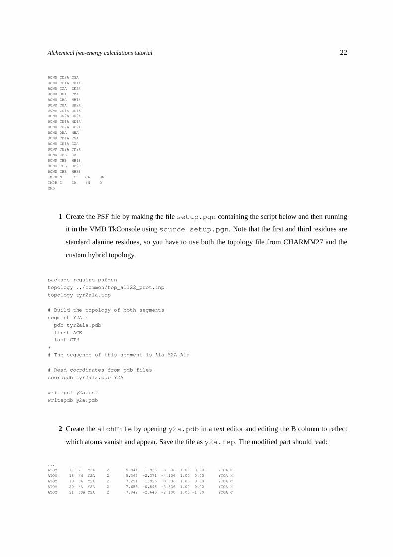
2 Create thealchFile by openingy2a.pdb in a text editor and editing the B column to reflect

which atoms vanish and appear. Save the file asy2a.fep . The modified part should read:

...

ATOM 17 N Y2A 2 5.841 -1.926 -3.336 1.00 0.00 YTOA N

ATOM 18 HN Y2A 2 5.362 -2.371 -4.106 1.00 0.00 YTOA H

ATOM 19 CA Y2A 2 7.291 -1.926 -3.336 1.00 0.00 YTOA C

ATOM 20 HA Y2A 2 7.655 -0.898 -3.336 1.00 0.00 YTOA H

ATOM 21 CBA Y2A 2 7.842 -2.640 -2.100 1.00 -1.00 YTOA C


ATOM 22 HB1A Y2A 2 7.014 -2.994 -1.485 1.00 -1.00 YTOA H

ATOM 23 HB2A Y2A 2 8.452 -3.487 -2.411 1.00 -1.00 YTOA H

ATOM 24 CGA Y2A 2 8.687 -1.679 -1.298 1.00 -1.00 YTOA C

ATOM 25 CD1A Y2A 2 8.856 -0.360 -1.739 1.00 -1.00 YTOA C

ATOM 26 HD1A Y2A 2 8.377 -0.028 -2.660 1.00 -1.00 YTOA H

ATOM 27 CE1A Y2A 2 9.640 0.531 -0.996 1.00 -1.00 YTOA C

ATOM 28 HE1A Y2A 2 9.771 1.557 -1.339 1.00 -1.00 YTOA H

ATOM 29 CZA Y2A 2 10.254 0.104 0.187 1.00 -1.00 YTOA C

ATOM 30 OHA Y2A 2 11.016 0.969 0.909 1.00 -1.00 YTOA O

ATOM 31 HHA Y2A 2 11.063 1.844 0.516 1.00 -1.00 YTOA H

ATOM 32 CD2A Y2A 2 9.302 -2.106 -0.115 1.00 -1.00 YTOA C

ATOM 33 HD2A Y2A 2 9.170 -3.132 0.227 1.00 -1.00 YTOA H

ATOM 34 CE2A Y2A 2 10.086 -1.215 0.627 1.00 -1.00 YTOA C

ATOM 35 HE2A Y2A 2 10.564 -1.547 1.548 1.00 -1.00 YTOA H

ATOM 36 CBB Y2A 2 7.842 -2.640 -2.100 1.00 1.00 YTOA C

ATOM 37 HB1B Y2A 2 7.014 -2.994 -1.485 1.00 1.00 YTOA H

ATOM 38 HB2B Y2A 2 8.452 -3.487 -2.411 1.00 1.00 YTOA H

ATOM 39 HB3B Y2A 2 8.687 -1.679 -1.298 1.00 1.00 YTOA C

ATOM 40 C Y2A 2 7.842 -2.640 -4.572 1.00 0.00 YTOA C

ATOM 41 O Y2A 2 7.078 -3.122 -5.407 1.00 0.00 YTOA O

...

3 Visualize the system containing the hybrid amino-acid. Run VMD with the following command:

vmd y2a.psf -pdb y2a.fep .

4 In the Graphics/Representations menu, set the coloring method toBeta . The appearing alanine

side chain should be colored blue and the tyrosine side chain should be red, while the backbone

and the two unperturbed alanine residues should be green. Compare the result with Figure7.

5 (Optional if using NAMD 2.7b2 or later) Remove spurious bonded force-field terms and add a

non–bonded exclusion list usingalchemify in the command prompt:

alchemify y2a.psf y2a-alch.psf y2a.fep

Use the resulting filey2a-alch.psf when performing thein vacuoFEP calculations.

6 You are now ready to prepare the hydrated system. Load the isolated tripeptide in VMD:vmd

y2a.psf y2a.pdb .

7 Open the Solvate interface (Extensions/Modeling/Add Solvation Box).

8 Define a cubic, 30×30×30 A3 water box: Uncheck the “Use Molecule Dimensions” box and the

“Waterbox Only”, set the minimum value ofx, y andz to−13 and their maximum to+13. Run

the plugin to create the filessolvate.psf andsolvate.pdb .


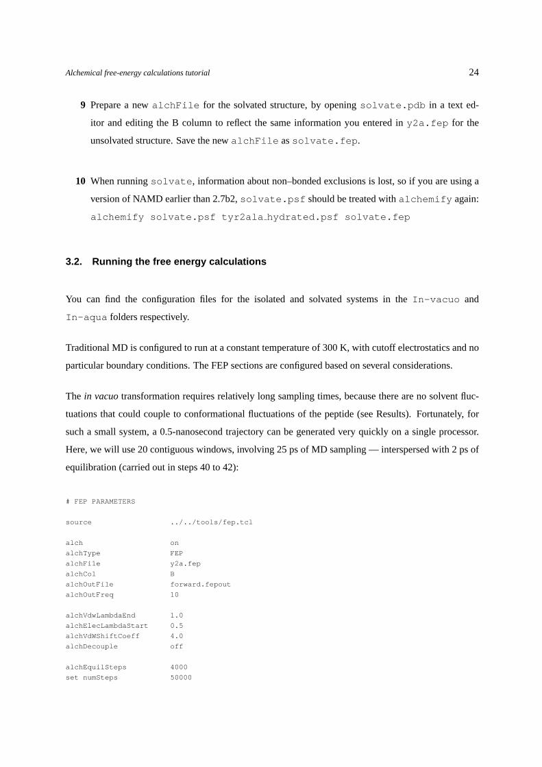
9 Prepare a newalchFile for the solvated structure, by openingsolvate.pdb in a text ed-

itor and editing the B column to reflect the same information you entered iny2a.fep for the

unsolvated structure. Save the newalchFile assolvate.fep .

10 When runningsolvate , information about non–bonded exclusions is lost, so if you are using a

version of NAMD earlier than 2.7b2,solvate.psf should be treated withalchemify again:

alchemify solvate.psf tyr2ala hydrated.psf solvate.fep

3.2. Running the free energy calculations

You can find the configuration files for the isolated and solvated systems in theIn-vacuo and

In-aqua folders respectively.

Traditional MD is configured to run at a constant temperature of 300 K, with cutoff electrostatics and no

particular boundary conditions. The FEP sections are configured based on several considerations.

The in vacuotransformation requires relatively long sampling times, because there are no solvent fluc-

tuations that could couple to conformational fluctuations of the peptide (see Results). Fortunately, for

such a small system, a 0.5-nanosecond trajectory can be generated very quickly on a single processor.

Here, we will use 20 contiguous windows, involving 25 ps of MD sampling — interspersed with 2 ps of

equilibration (carried out in steps 40 to 42):

# FEP PARAMETERS

source ../../tools/fep.tcl

alch on

alchType FEP

alchFile y2a.fep

alchCol B


alchOutFreq 10




alchDecouple off

alchEquilSteps 4000

set numSteps 50000



We will use a similar strategy for the solvated system, albeit with a somewhat larger time step. In

each window, the system is equilibrated overalchEquilSteps MD steps,viz. here 100 steps, prior

to 400 steps of data collection, making a total of 0.5 ps of MD sampling. Altogether, the alchemical

transformation is carried out over 10 ps, and the backward transformation over the same time. (carried

out in steps 43 to 45)

# FEP PARAMETERS


alch on

alchType FEP


alchCol B

alchOutFile forward-off.fepout

alchOutFreq 10




alchDecouple off

alchEquilSteps 100

set numSteps 500


1 Navigate to theIn-vacuo folder.

2 First, runequilibration.namd in the command prompt:

namd2 equilibration.namd > equilibration.log

3 Next, repeat the above command forforward.namd andbackward.namd to generate the

required data files for analysis.

4 Now navigate to theIn-aqua folder. Note that the difference between the files suffixed by-on

and those by-off lies in thealchDecouple switch. For now you will work with the files with

suffix off .


ThealchDecouple switch determines whether or not the vanishing and appearing moieties interact

with each other. Switching decoupling off in this example causes the perturbed moieties to interact not

only with the environment but also with each other. We discuss the use of this option at greater length in

the Results section.

5 Perform the equilibration run.

6 Perform the forward and backward simulations.

3.3. Results

Figure 8: Results for the Tyr→ Ala mutations in water and in vacuum, in the Ala–Tyr–Ala blocked tripeptide.

The difference between the corresponding free-energy changes yields the relative hydration free energy of Ala–

Tyr–Ala with respect to (Ala)3. The transformation in vacuum accounts for intramolecular interactions between the

perturbed moieties,i.e. alchDecouple off . As a basis of comparison and a consistency check, the results of

decoupling-recoupling simulations,i.e. forward (dark solid line) and backward (dark dashed line) transformations

with decouple on , in water are shown. Because this option ignores intra-perturbed interactions, it also obviates

the need for separate gas-phase simulations.

1 Usegrep to extract the free energy profiles from thealchOutFile s generated by your forward

and backward simulations.

The∆G(λ) curves for both simulations, as well as an alternate method, are shown in Figure8. Using

an adapted protocol for each of the two mutations, the free energy difference for the hydrated state is


+11.7 kcal/mol, and+4.0 kcal/mol for the isolated state; your values may be slightly different due to

the very short simulation times used here. Using the thermodynamic cycle of Figure6, one may write:

∆∆G = ∆G2alch. −∆G1

alch. = ∆G2hydr. −∆G1

hydr.

The net solvation free energy change∆∆G for the Ala–Tyr–Ala→ (Ala)3 transformation is found to

be +7.7 kcal/mol. Alternately, a single decoupling/recoupling simulation indicates a hydration free

energy difference of+8.1 kcal/mol, in agreement with the double annihilation scheme. This result may

be related to the differential hydration free energy of side–chain analogues,i.e. the difference in the

hydration free energy of methane andp–cresol, that is, respectively, 1.9 + 6.1 =+8.0 kcal/mol [20,

21]. Interestingly enough, Scheraga and coworkers have estimated the side–chain contribution for this

mutation to be equal to +8.5 kcal/mol [22].

This very close agreement with experimental determinations based on side–chain analogues, as well as

other computational estimates, may be in part coincidental or due to fortuitous cancellation of errors.

Indeed, some deviation could be expected due to environment effects —viz. the mutation of a residue

embedded in a small peptide chainversusthat of an isolated, prototypical organic molecule[23] — and,

to a lesser extent, the limited accuracy of empirical force fields. The first explanation may be related

to the concept of “self solvation” of the side chain. Here, the tyrosyl fragment is not only solvated

predominantly by the aqueous environment, but also, to a certain degree, by the peptide chain, which,

under certain circumstances, can form hydrogen bonds with the hydroxyl group.

Moreover, it should be noted that even for a small and quickly relaxing system such as the hybrid tripep-

tide, convergence of the FEP equation requires a significant time. In some cases, very short runs may

give better results than moderately longer ones, because the former provide a local sampling around the

starting configuration, while the latter start exploring nearby conformations, yet are not long enough to

fully sample them.

In general, whether or not intramolecular interactions ought to be perturbed —i.e. alchDecouple

set tooff or on , respectively — requires careful attention. As has been seen here, ignoring perturbed

intramolecular interactions is computationally advantageous in the sense that it obviates the need for

the gas-phase simulation depicted in Figure7. This choice is fully justified in the case of rigid, or

sufficiently small molecules. If, however, the system of interest can assume multiple conformations,

settingalchDecouple to on may no longer be appropriate. This is due to the fact that on account


of the environment, specifically its permittivity, the conformational space explored in the low-pressure

gaseous phase is likely to be different from that in an aqueous medium.

In all cases, visualizing MD trajectories is strongly advisable if one wishes to understand the behavior of

the system and to solve possible sampling issues. Looking at the present tyrosine-to-alanine trajectories,

it appears that the main conformational degree of freedom that has to be sampled is the rotation of the

tyrosine hydroxyl group. Convergence is actually faster for the solvated system than for the tripeptide

in vacuum, because fluctuations of the solvent help the tyrosine side chain pass the rotational barriers,

which does not happen frequently in vacuum.


4. Binding of a potassium ion to 18–crown–6

For this final example, we will go through the theoretical framework for measuring standard binding free

energies, using the simple example of a potassium ion associated to a crown ether, namely 18–crown–6.

18–crown–6:K+ has been investigated previously by means of molecular simulations. In their pioneering

work, Dang and Kollman evaluated the potential of mean force delineating the reversible separation of

the ion from the ionophore [24, 25]. Alchemical FEP, however, has proven over the years [7] to constitute

a method of choice for measuringin silico host:guest binding free energies.

OOO

OOO

aq.

Ka

OOO

OOO

aq.

K+aq. K+

"0"aq.

G∆ 1annihil

G∆ rest

+

OOO

OOO

aq.

+

OOO

OOO

aq.

"0"

G∆ annihil2

Figure 9: Thermodynamic cycle delineating the reversible association of a potassium ion to the 18–crown–6

crown ether in an aqueous environment. Binding of the ion to the ionophore is characterized by the association

constantKa and can be measured directly by means of a potential of mean force–like calculation. Alternatively,

FEP can be employed to annihilate, or create the potassium ion both in the free and in the bound states. It follows

from the latter that∆Gbinding = −1/β lnKa = ∆G1annihil−∆G2

annihil. To prevent the cation from moving astray

when it is only weakly coupled to the crown ether,i.e. at the very end of the annihilation transformation, or at

the beginning of the creation transformation, positional restraints ought to be enforced, contributing∆Grest to the

overall binding free energy.

Here, the standard binding affinity of a potassium ion towards 18–crown–6 will be determined using

this approach and following the thermodynamic cycle of Figure9, wherein the alkaline ion undergoes a

double annihilation [26], in its free and bound states.


4.1. System setup

Double annihilation refers to the ion being annihilated both in the free and in the bound state. In other

words, we have to build two different molecular systems,viz. . a potassium ion in a water bath and the

complex 18–crown–6:K+, also in a water bath.

The topology of 18–crown–6 is supplied in18crown6.top . In addition, the initial coordinates of the

ionophore are provided18crown6.pdb . We will use these files to set up the host-guest complex. The

first step of the setup is to build the PSF file for the host.

1 In the VMD TkConsole, navigate to the folder04.Binding-of-a-potassium-ion-to-18-crown-6

and use the following script:


topology 18crown6.top

segment 18C6 { pdb 18C6.pdb }

coordpdb 18crown6.pdb

writepsf 18crown6.psf

2 Now you will build the PDB and PSF files for the guest. Without exiting VMD, enter the following

script in the TkConsole:

resetpsf

topology top_all22_prot.inp

segment POT { residue 0 POT }

writepdb potassium.pdb

writepsf potassium.psf

3 Merge the 18–crown–6 and potassium ion into a single PSF and PDB file by issuing the following

commands in the VMD TKConsole:

resetpsf

readpsf 18crown6.psf

coordpdb 18crown6.pdb

readpsf potassium.psf

coordpdb potassium.pdb

writepsf complex.psf

writepdb complex.pdb


Now, we will center the ion with respect to the center of mass of 18–crown–6.

4 Open in VMD the filescomplex.psf and complex.pdb . Measure the center of mass of

18–crown–6, then move the potassium ion to the center, using

set sel [atomselect top "segname 18C6"]

set vec [measure center $sel]

set sel2 [atomselect top "segname POT"]

$sel2 moveby $vec

5 Write a new pdb file for the system:writepdb complex new.pdb

Before you immerse the complex in water, recall that the free energy of the system is dependent on the

size of the hydration box. The size-dependence correction imposed by the long-range nature of charge–

dipole interactions is expected to cancel out if the dimensions of the simulation cell are identical for the

two vertical legs of the thermodynamic cycle of Figure9. In both cases, a box of dimension 28× 28×

28 A3 appears to constitute a reasonable compromise in terms of cost-effectiveness.

6 We now proceed to preparing the hydrated system. Loadcomplex.psf and

complex new.pdb into VMD. Use the solvate plugin to create a water box of the

recommended dimensions. Uncheck ”Use Molecule Dimensions” and ”Waterbox Only” before

running. You will obtainsolvate.psf andsolvate.pdb . Move these files to the folder

labeledcomplex .

7 You must solvate also the lone potassium ion. Start a new session of VMD. LoadPOT.psf

andPOT.pdb into VMD. Repeat the solvation step described previously tosolvate.psf and

solvate.pdb . Move these files to the folder labeledpotassium .

8 Using a text editor, make analchFile for each of the two systems you have created by editing

their respective PDB files. Give the vanishing potassium ion a value of -1 in the B column, and

then save the new files assolvate.fep in their respective folders.


4.2. Running the free energy calculations

We will minimize each system and then carry out equilibration, as a preamble to the free-energy calcu-

lations. In the case of the hydrated 18–crown–6:K+ complex, this thermalization step will be utilized to

appreciate how strongly bound is the guest in its dedicated binding site.

Equilibrium MD will be run for both systems at a constant temperature of 300 K with a damping coef-

ficient of 1 ps−1, and pressure of 1 bar, using PME electrostatics. TherigidBonds option will be set

to all to increase the integration time step of 2 fs. To impose isotropic fluctuations of the periodic box

dimensions, theflexibleCell variable will be set tono . The trajectory will be saved in a DCD file

with a frequency ofe.g.100 time steps.

1 At the command prompt, navigate to the foldercomplex . Run the minimization by entering

namd2 minimization.namd > minimization.log .

2 Run the equilibration by entering

namd2 equilibration.namd > equilibration.log .

3 Repeat the minimization and equilibration steps for the unbound potassium ion in thepotassium

folder.

To measure how the position of alkaline ion fluctuates in the ionophore, the trajectory of the 18–crown–

6:K+ complex can be loaded and the coordinates of the system aligned with respect to the heavy atoms

of the crown ether.

4 Start a session of VMD and loadsolvate.psf andsolvate.pdb in the complex folder.

Then load into the molecule the trajectorysolvate.dcd .

5 The alignment and calculation of the distance separating the center of mass of 18–crown–6 from

the ion every frame can be performed using the following simple TCL script:

set outfile [open COM-ion.dat w]


set nf [molinfo top get numframes]

set all [atomselect top "all"]

set crown [atomselect top "resname 18C6 and noh"]

set crown0 [atomselect top "resname 18C6 and noh" frame 0]

set ion [atomselect top "segname POT"]

for { set i 1 } { $i <= $nf } { incr i } {

$all frame $i

$crown frame $i

$ion frame $i

$all move [measure fit $crown $crown0]

$crown update

$ion update

set COM [measure center $ion weight mass]

set dist [expr sqrt(pow([lindex $COM 0],2)+pow([lindex $COM 1],2)+pow([lindex $COM 2],2))]

puts $outfile [format "%8d %8f" $i $dist]

}

close $outfile

The output file lists two columns of numbers, the first being the frame number and the second being the

distance of the ion from the center of mass of 18–crown–6. You can use any plotting software to plot a

graph of the distance against frame number. The maximum fluctuation in the distance between the center

of mass of 18–crown–6 and the potassium ion will serve as the basis for a positional restraint introduced

in the subsequent free-energy calculation, in which the ion is annihilated in its bound state.

6 Now we move on to the free energy calculations. Navigate to thecomplex folder and inspect the

forward.namd configuration file.

Look at the FEP section. An identical sampling strategy will be used for the annihilation of the potassium

ion in the free and in the bound state. Here, use will be made of 32 equally spaced intermediate states:

# FEP PARAMETERS


alch on

alchType FEP


alchCol B

alchOutFreq 10





alchVdwShiftCoeff 5.0

alchdecouple on

alchEquilSteps 50

set numSteps 200

set dLambda 0.03125

runFEP 0.0 1.0 $dLambda $numSteps

We will employ the COLVARS module of NAMD to enforce a positional restraint by means of an isotropic

harmonic potential —i.e. an external potential that confines the ion within a sphere of given radius,

centered about the center of mass of the ionophore. To do so, the following two lines have been added to

the NAMD configuration file:

colvars on

colvarsConfig COMCOM.in

In addition, a separate, dedicatedcolvarsConfig file, COMCOM.in, has been written to instruct

COLVARS of the positional restraint to be enforced:

colvarsTrajFrequency 100

colvarsRestartFrequency 100

colvar {

name COMDistance

width 0.1

lowerboundary 0.0

upperboundary 0.5

lowerWallConstant 100.0

upperWallConstant 100.0

distance {

group1 {

atomnumbers { 43 }

}

group2 {

atomnumbers { 1 4 5 8 11 12

15 18 19 22 25 26

29 32 33 36 39 40 }


}

}

}

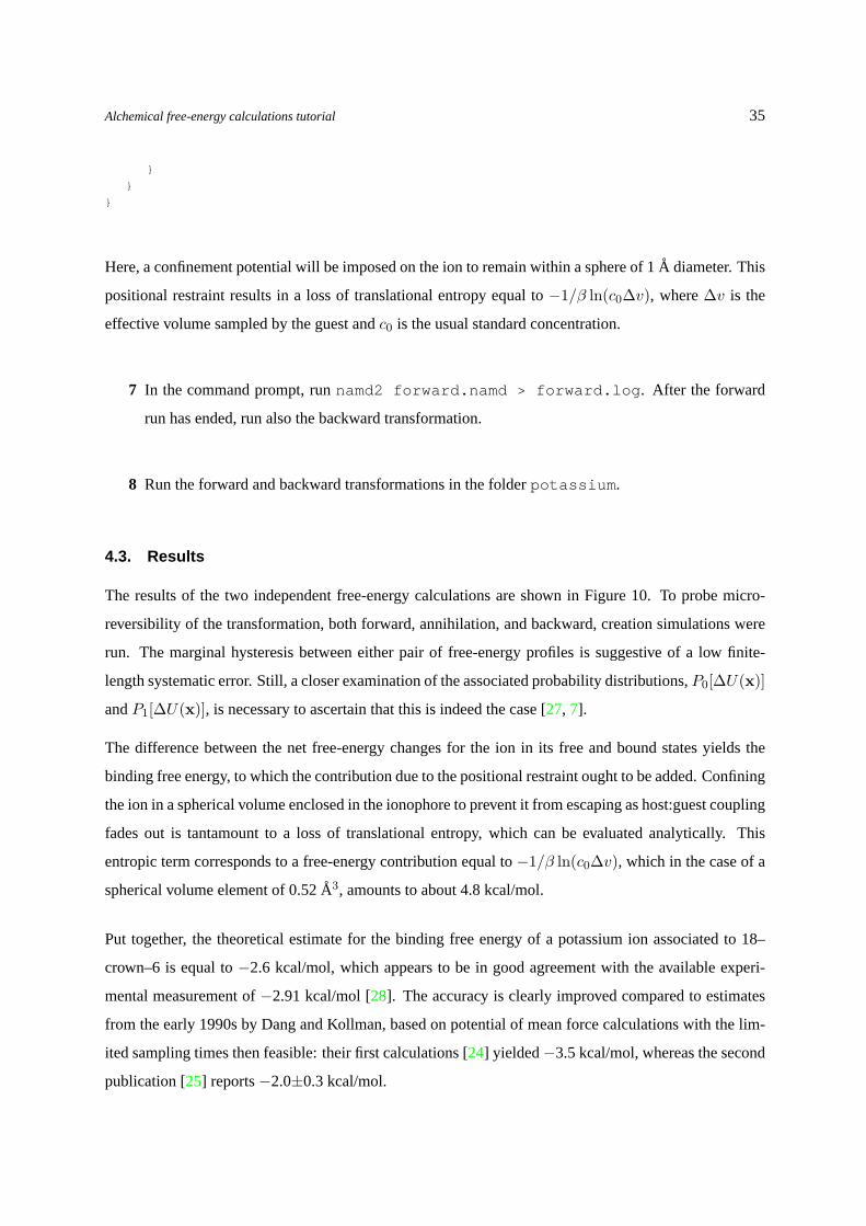
Here, a confinement potential will be imposed on the ion to remain within a sphere of 1A diameter. This

positional restraint results in a loss of translational entropy equal to−1/β ln(c0∆v), where∆v is the

effective volume sampled by the guest andc0 is the usual standard concentration.

7 In the command prompt, runnamd2 forward.namd > forward.log . After the forward

run has ended, run also the backward transformation.

8 Run the forward and backward transformations in the folderpotassium .

4.3. Results

The results of the two independent free-energy calculations are shown in Figure10. To probe micro-

reversibility of the transformation, both forward, annihilation, and backward, creation simulations were

run. The marginal hysteresis between either pair of free-energy profiles is suggestive of a low finite-

length systematic error. Still, a closer examination of the associated probability distributions,P0[∆U(x)]

andP1[∆U(x)], is necessary to ascertain that this is indeed the case [27, 7].

The difference between the net free-energy changes for the ion in its free and bound states yields the

binding free energy, to which the contribution due to the positional restraint ought to be added. Confining

the ion in a spherical volume enclosed in the ionophore to prevent it from escaping as host:guest coupling

fades out is tantamount to a loss of translational entropy, which can be evaluated analytically. This

entropic term corresponds to a free-energy contribution equal to−1/β ln(c0∆v), which in the case of a

spherical volume element of 0.52A3, amounts to about 4.8 kcal/mol.

Put together, the theoretical estimate for the binding free energy of a potassium ion associated to 18–

crown–6 is equal to−2.6 kcal/mol, which appears to be in good agreement with the available experi-

mental measurement of−2.91 kcal/mol [28]. The accuracy is clearly improved compared to estimates

from the early 1990s by Dang and Kollman, based on potential of mean force calculations with the lim-

ited sampling times then feasible: their first calculations [24] yielded−3.5 kcal/mol, whereas the second

publication [25] reports−2.0±0.3 kcal/mol.


Figure 10: Free-energy change for the double annihilation of a potassium ion in its bound state, associated to

18–crown–6 (black solid line and pluses for the forward transformation, black dashed line and circles for the

backward transformation), and in its free state, in a bulk aqueous environment (light solid line and pluses for the

forward transformation, red dashed line and circles for the backward transformation). The difference atλ = 1,

between the net free-energy changes,∆G1annihil − ∆G2

annihil, viz. 54.1− 61.5 = -7.4 kcal/mol, corresponds to

the binding free energy,i.e.−1/β lnKa, to which the contribution due to the confinement of the ion in the crown

ether,viz.4.8 kcal/mol, ought to be added. The resulting standard binding free energy of−2.6 kcal/mol is in good

agreement with the experimental measurement of−2.91 kcal/mol of Michaux and Reisse [28].

Role of confinement potentials

Introduction of a positional restraint by means of the COLVARS module can be substituted

by the addition of pseudo bonds between the ionophore and the alkaline cation. These

bonds, aimed at tethering the ion as its coupling to the crown ether vanishes, are declared in

the NAMD configuration file by:

extraBonds yes

extraBondsFile restraints.txt

The reader is invited to refer to the NAMD user’s guide for the syntax employed for defin-

ing pseudo bonds in the externalextraBondsFile file, and verify that following this

route and subsequently measuring the free-energy cost incurred for fading out these pseudo

bonds —i.e. by zeroing out reversibly the associated force constants, the aforementioned

contribution due to the loss of translational entropy can be recovered.

Finite-length bias

For each individualλ-intermediate state, monitor the probability distribution functions

P0[∆U(x)] andP1[∆U(x)], and verify that the systematic error due to the finite length

of the free-energy calculation [7] is appreciably small.


Acknowledgements

Development of this tutorial was supported by the National Institutes of Health (P41-RR005969 - Re-

source for Macromolecular Modeling and Bioinformatics).

References

[1] Dixit, S. B.; Chipot, C., Can absolute free energies of association be estimated from molecular

mechanical simulations ? The biotin–streptavidin system revisited,J. Phys. Chem. A2001, 105,

9795–9799.

[2] Phillips, J. C.; Braun, R.; Wang, W.; Gumbart, J.; Tajkhorshid, E.; Villa, E.; Chipot, C.; Skeel, L.;

Schulten, K., Scalable molecular dynamics with NAMD , J. Comput. Chem.2005, 26, 1781–1802.

[3] Bhandarkar, M.; Brunner, R.; Buelens, F.; Chipot, C.; Dalke, A.; Dixit, S.; Fiorin, G.; Freddolino,

P.; Grayson, P.; Gullingsrud, J.; Gursoy, A.; Hardy, D.; Harrison, C.; Henin, J.; Humphrey, W.;

Hurwitz, D.; Krawetz, N.; Kumar, S.; Nelson, M.; Phillips, J.; Shinozaki, A.; Zheng, G.; Zhu, F.

NAMD user’s guide, version 2.7. Theoretical biophysics group, University of Illinois and Beckman

Institute, Urbana, IL, July 2009.

[4] Born, M., Volumen und Hydratationswarme der Ionen,Z. Phys.1920, 1, 45–48.

[5] Chipot, C.; Pearlman, D. A., Free energy calculations. The long and winding gilded road,Mol. Sim.

2002, 28, 1–12.

[6] Chipot, C. Free energy calculations in biological systems. How useful are they in practice? in

New algorithms for macromolecular simulation, Leimkuhler, B.; Chipot, C.; Elber, R.; Laaksonen,

A.; Mark, A. E.; Schlick, T.; Schutte, C.; Skeel, R., Eds., vol. 49. Springer Verlag, Berlin, 2005,

pp. 183–209.

[7] Chipot, C.; Pohorille, A., Eds.,Free energy calculations. Theory and applications in chemistry and

biology, Springer Verlag, 2007.

[8] Gao, J.; Kuczera, K.; Tidor, B.; Karplus, M., Hidden thermodynamics of mutant proteins: A molec-

ular dynamics analysis,Science1989, 244, 1069–1072.


[9] Pearlman, D. A., A comparison of alternative approaches to free energy calculations,J. Phys. Chem.

1994, 98, 1487–1493.

[10] Humphrey, W.; Dalke, A.; Schulten, K., VMD: visual molecular dynamics,J. Mol. Graph.1996,

14, 33–8, 27–8.

[11] Pearlman, D. A.; Kollman, P. A., The overlooked bond–stretching contribution in free energy per-

turbation calculations,J. Chem. Phys.1991, 94, 4532–4545.

[12] Zacharias, M.; Straatsma, T. P.; McCammon, J. A., Separation-shifted scaling, a new scaling

method for Lennard-Jones interactions in thermodynamic integration,J. Chem. Phys.1994, 100,

9025–9031.

[13] Beutler, T. C.; Mark, A. E.; van Schaik, R. C.; Gerber, P. R.; van Gunsteren, W. F., Avoiding sin-

gularities and neumerical instabilities in free energy calculations based on molecular simulations,

Chem. Phys. Lett.1994, 222, 529–539.

[14] Pitera, J. W.; van Gunsteren, W. F., A comparison of non–bonded scaling approaches for free energy

calculations,Mol. Sim.2002, 28, 45–65.

[15] Hummer, G.; Pratt, L.; Garcia, A. E., Free energy of ionic hydration,J. Phys. Chem.1996, 100,

1206–1215.

[16] Marcus, Y., Thermodynamics of solvation of ions: Part 5. Gibbs free energy of hydration at 298.15

K, J. Chem. Soc. Faraday Trans.1991, 87, 2995–2999.

[17] Straatsma, T. P.; Berendsen, H. J. C., Free energy of ionic hydration: Analysis of a thermodynamic

integration technique to evaluate free energy differences by molecular dynamics simulations,J.

Chem. Phys.1988, 89, 5876–5886.

[18] Kollman, P. A., Free energy calculations: Applications to chemical and biochemical phenomena,

Chem. Rev.1993, 93, 2395–2417.

[19] MacKerell, Alexander D; Feig, Michael; Brooks, Charles L, Extending the treatment of backbone

energetics in protein force fields: limitations of gas-phase quantum mechanics in reproducing pro-

tein conformational distributions in molecular dynamics simulations,J. Comput. Chem.2004, 25,

1400–1415.


[20] Dixit, S. B.; Bhasin, R.; Rajasekaran, E.; Jayaram, B., Solvation thermodynamics of amino acids.

Assessment of the electrostatic contribution and force-field dependence,J. Chem. Soc., Faraday T

rans.1997, 93, 1105–1113.

[21] Shirts, M. R.; Pande, V. S., Solvation free energies of amino acid side chain analogs for common

molecular mechanics water models,J. Chem. Phys.2005, 122, 134508.

[22] Ooi, T.; Oobatake, M.; Nemethy, G.; Scheraga, H. A., Accessible surface areas as a measure of

the thermodynamic parameteres of hydration of peptides,Proc. Natl. Acad. Sci. USA1987, 84,

3086–3090.

[23] Konig, G.; Boresch, S., Hydration free energies of amino acids: why side chain analog data are not

enough,J. Phys. Chem. B2009, 113, 8967–8974.

[24] Dang, Liem X.; Kollman, Peter A., Free energy of association of the 18-crown-6:K+ complex in

water: a molecular dynamics simulation,J. Am. Chem. Soc.1990, 112, 5716–5720.

[25] Dang, Liem X.; Kollman, Peter A., Free Energy of Association of the K+:18-Crown-6 Complex in

Water: A New Molecular Dynamics Study,J. Phys. Chem.1995, 99, 55–58.

[26] Gilson, M. K.; Given, J. A.; Bush, B. L.; McCammon, J. A., The statistical-thermodynamic basis

for computation of binding affinities: A critical review,Biophys. J.1997, 72, 1047–1069.

[27] Zuckerman, D.M.; Woolf, T.B., Theory of a systematic computational error in free energy differ-

ences,Phys. Rev. Lett.2002, 89, 180602.

[28] Michaux, Gabriel; Reisse, Jacques, Solution thermodynamic studies. Part 6. Enthalpy-entropy com-

pensation for the complexation reactions of some crown ethers with alkaline cations: a quantitative

interpretation of the complexing properties of 18-crown-6,J. Am. Chem. Soc.1982, 104, 6895–

6899.

View publication statsView publication stats

https://www.researchgate.net/publication/265004753

in silico alchemy - researchgate.net · abstract this tutorial explains how namd and related tools...

Documents