in-season retail sales forecasting using survival models

Volume 30 (2), pp. 59–71

http://orion.journals.ac.za

ORiONISSN 0529-191-X

c©2014

In-season retail sales forecasting using survivalmodels

M Hattingh∗ DW Uys†

Received: 26 February 2013; Revised: 18 November 2013; Accepted: 21 November 2013

Abstract

A large South African retailer (hereafter referred to as the Retailer) faces the problem ofselling out inventory within a specified finite time horizon by dynamically adjusting productprices, and simultaneously maximising revenue. Consumer demand for the Retailer’s fashionmerchandise is uncertain and the identification of products eligible for markdown is thereforeproblematic. In order to identify products that should be marked down, the Retailer forecastsfuture sales of new products. With the aim of improving on the Retailer’s current salesforecasting method, this study investigates statistical techniques, viz. classical time seriesanalysis (Holt’s smoothing method) and survival analysis. Forecasts are made early in theproduct life cycle and results are compared to the Retailer’s existing forecasting method.Based on the mean squared errors of predictions resulting from each method, the mostaccurate of the methods investigated is survival analysis.

Key words: Retail sales forecasting, survival analysis, time series analysis, Holt’s smoothing method.

1 Introduction

A large South African retailer that aims to provide affordable merchandise to the lower-and middle-income target market is considered. The Retailer offers a vast selection ofdifferent products, ranging from shoes and clothing to cell phones and home decorations.A large proportion of merchandise that the Retailer sells consists of fashion items, of whichthe demand is dependent on seasonal trends and consumer sentiment. For this reason,it is difficult to estimate future seasonal demand. For seasonal products, new stock isbought from overseas suppliers every season. For this particular Retailer, this is a once-offtransaction, and once the stock has been ordered by the Retailer’s buyers, no changes canbe made, irrespective of the product’s sales performance.

∗Business Intelligence and Actuarial Synthesis Team, Metropolitan Retail: CFO Division, Building 6/1,Parc du Cap, Mispel Road, Bellville, 7530.†Corresponding author: Department of Statistics and Actuarial Science, University of Stellenbosch,

Private Bag X1, Matieland, 7602, email: [email protected]

http://dx.doi.org/10.5784/30-2-153

59

http://orion.journals.ac.za

[email protected]

http://dx.doi.org/10.5784/30-2-153

60 M Hattingh & DW Uys

Demand for the Retailer’s products is price-elastic due to the nature of the target market.Periodic price cuts throughout the season stimulate sales for products that do not sellout satisfactorily. However, the Retailer should avoid marking down products for whichconsumers are willing to pay full price. It is important to identify which products should bemarked down at an early stage because if markdowns occur too late, inefficient occupationof shelf space may lead to a decrease in revenue.

The problem that the Retailer faces corresponds to the widely researched field of markdownoptimisation, originally conducted by Kincaid and Darling (1963). Markdown optimisationdeals with the problem of maximising expected total revenue by continuously adjustingprices, given that sales may only take place within a finite time horizon (Gallego & VanRyzin 1994). A brief overview of the literature in this field and a discussion of why atraditional approach to markdown optimisation is inappropriate in the case of the Retailerare given here. Subsequently, a discussion of the methods used in the study is given.

1.1 Stochastic demand models

As an input in the markdown optimisation model, consumer demand needs to be mod-elled, either deterministically or stochastically. In stochastic models of consumer demand,consumer demand can either be a random variable or a function of a random variable.An example of the former is to model sales of a specific product over time as a Poissoncounting process with transition intensity inversely proportional to price (Chatwin 2000).The objective is then to maximise the expected revenue under the assumed distribution.Under the Poisson model, the maximum expected revenue is a non-decreasing, concavefunction of remaining inventory over time to the end of the season, and the optimal priceis continuously decreasing (Chatwin 2000).

Mantrala and Rao (2001) define a model where demand is a function of both deterministicand stochastic variables. The function is given by

Dtj = αtM

(PfPtj

)γtεt,

where

Dtj is consumer demand for product j at time t at price Ptj ,αt is a seasonal factor at time t,Pf is the full price of the product, charged at the beginning of the season,M is the total seasonal demand at price Pf ,γt is a function of the sensitivity at time t of consumer demand to a change in

price, andεt is a random variable with a continuous time lognormal distribution (i.e. the

random disturbance component takes the form of geometric Brownian Mo-tion).

The estimation of parameters for a stochastic model requires an extensive amount of data.For the model described above, the sensitivity parameter γt varies over time, and can onlybe estimated if there are sufficient observed values of Dtj for all values of t and j.

In-season retail sales forecasting using survival models 61

Data available to the particular Retailer investigated in this study only provides informa-tion on the effect of late price changes (if any) on consumer demand. In other words, thereare

• many observed values of Dtj if Ptj = Pf for all values of t,

• very few observed values of Dtj if Pf 6= Ptj for large values of t, or

• no observed values of Dtj of Pf 6= Ptj for small values of t.

Since model fitting requires a sufficient number of observed values for Dtj for all valuesof t and j, γt cannot be estimated accurately based on the available data. If a stochasticmodel was to be used to optimise markdowns, subjective assumptions would be requiredabout the form of γt. These assumptions may be inaccurate, and resulting markdowndecisions may potentially lead to losses in revenue.

A further disadvantage of the stochastic approach is that it often requires the assumptionof independence of sales quantities in consecutive weeks, which is unlikely to be valid(Lobel & Perakis 2010).

Given the limited nature of the available data for the Retailer investigated, it is notfeasible to apply markdown optimisation in its traditional sense to the Retailer’s markdowndecision problem. However, the data may be useful for predicting what demand will beassuming that the price remains constant. Using the previous notation, a model for Dtj

can be developed, assuming a constant price, since there are many observed values ofDtj where Ptj = Pf . Even though such a model would not be useful for determining theoptimal time and magnitude of markdowns, it may nevertheless help in identifying whichproducts should be marked down.

Therefore, instead of investigating ways of optimising markdowns, this study focuses onthe question of whether markdowns for particular new products are necessary at all. Theidentification of products eligible for markdown is done by means of in-season sales fore-casting of newly launched products, assuming no price change. Sales forecasts providesinformation as to whether the products considered will sell out within the specified timehorizon if the price remains the same. If not, the product is flagged for markdown.

1.2 The Retailer’s approach to markdown identification

To assist with decisions regarding the markdown of products, an early indication of likelyfuture sales performance is needed. The Retailer therefore predicts the remaining shelf lifeof products shortly after the commencement of sales based on a simple heuristic method,which is hereafter referred to as the forward cover method. The concept of forward cover,also known as “weeks of supply”, is widely used in different forms across the retail industry(Meckin 2007). The forward cover is defined as a measure of the number of weeks’ worthof inventory in stock at any particular time (Chase et al. 2008). The variation of forwardcover used by the Retailer is based on the assumption that sales will remain constant overthe entire remaining shelf life of the product. The constant rate of future sales is assumedto be an average of the previous 5 weeks of sales.


The forward cover calculated in week n is defined by

Fn =Cn

15

∑4i=0 Sn−i

,

where

Ci is the closing inventory for week i, andSi is the quantity of products sold during week i.

This calculation is done on a weekly basis, starting as soon as sufficient sales data areavailable. Products that are not expected to sell out within the allowed time horizon arethen identified as being eligible for markdown.

In this study, two alternative forecasting methods (described in §1.4.) are investigatedwith the aim of improving on the accuracy of the forward cover method. Ideally, theremaining future shelf life of products should be forecasted in a methodical, quantitativemanner. Furthermore, the forecasting model should be capable of:

1. producing forecasts of future sales on a weekly basis,

2. using very little data as the basis for the forecasts,

3. using as much as possible of the information underlying the available data, and

4. using knowledge of trends in past data (on sales of similar products) as a referenceto estimate sales of a new product.

1.3 Forecasting methods

Two forecasting models are proposed to predict future sales, namely time series analysisand survival analysis.

1.3.1 Time series analysis

A number of time series techniques have been used for sales forecasting, including Au-toregressive Integrated Moving Average (ARIMA) models, Bayesian forecasting modelsand exponential smoothing models. Most of these methods require estimation of severalparameters. In this study, an early indicator of future product success is needed. Fore-casts are required after only eight weeks of initial sales. Since only eight data points areavailable on which to base forecasts, a model with as few as possible required parameterestimates is needed.

Holt’s smoothing method for exponential trend was used in this study, since there wasno significant seasonality over the short time period observed and inventory typicallydiminishes faster than straight-line decay. Forecasts are obtained for the weekly closinginventory percentages. To obtain an estimate for the forward cover, the number of weeksuntil the forecasted inventory is less than 1% of total inventory is established.

1.3.2 Survival analysis

The theory of survival analysis considers the time to occurrence of a particular event. Pos-sible events include the time of death in clinical trials, the length of stay in hospital until


discharge, or even how long it takes before a light bulb fuses. In the past, practical appli-cations of survival analysis principles have mainly been in the actuarial field, but survivalanalysis has increasingly been used in non-traditional fields, including the manufacturingindustry (Berry 2009).

The general survival function S(t) is defined as

S(t) = P (T > t).

It is the probability that a response variable T ≥ 0 exceeds time t. The survival functiondenotes the probability that a subject will survive for a minimum period of t time units.In the case where the probability of survival of a subject is dependent on the age of thesubject, the survival function may be written as a function of age. The probability that asubject currently aged x will survive for a minimum period of t time units is expressed as

ptx = Sx(t) = P (Tx ≥ t).

The hazard function, µ(t), is defined as the instantaneous rate at which deaths occur,conditional on no previous deaths occurring. The hazard function is given by

µ(t) = lim∆t→0

P (t < Tx < t+ ∆t | Tx > t)

∆t=fx(t)

Sx(t),

where fx(t) is the probability density function of the future lifetime, Tx, of a subject agedx (Cox & Oakes 1984). The survival function, ptx, is hence defined as a function of theintegrated hazard function and is given by

ptx = exp

(−∫ x+t

xµ(s) ds

).

In the context of sales forecasting, the future shelf life of products is considered, i.e. theresponse variable Tx is defined as the time until sale of a product given that the producthas been on the shelf for x weeks. The probability of a particular product being sold inany given week is considered analogous to the probability of death. The probability that aproduct is sold between week x and x+1, given that it is not sold by week x, is representedby

qx = 1− p1x = 1− exp

(−∫ x+1

xµ(s) ds

).

The application of survival models in retail sales forecasting is potentially useful because:

1. No distributional assumptions are needed in the model. The model relies solely ondata and the result is an empirically derived set of mortality rates that capture allinformation contained in past data without the need for parametric formulae.

2. The results of the model depend on a mix between information obtained from pastdata and the latest sales data of new products.


1.4 Cross validation

In order to test the validity of the suggested models, a subset of 11 products was left outof the data analysis and used as test observations. Afterwards, all models were applied tothe chosen 11 products. This allowed direct comparison of the two forecasting techniqueswith the forward cover method.

2 Survival analysis methodology

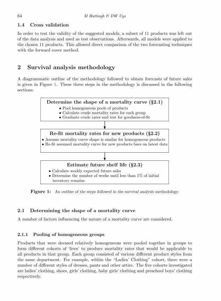
A diagrammatic outline of the methodology followed to obtain forecasts of future salesis given in Figure 1. These three steps in the methodology is discussed in the followingsections.

Re-fit mortality rates for new products (§2.2)

• Re-fit assumed mortality curve for new products baes on latest data

Determine the shape of a mortality curve (§2.1)

• Calculate crude mortality rates for each group

• Assume mortality curve shape is similar for homogeneous products

• Graduate crude rates and test for goodness-of-fit

• Pool homogeneous pools of products

Estimate future shelf life (§2.3)• Calculate weekly expected future sales• Determine the number of weeks until less than 1% of initial

inventory remains

Figure 1: An outline of the steps followed in the survival analysis methodology.

2.1 Determining the shape of a mortality curve

A number of factors influencing the nature of a mortality curve are considered.

2.1.1 Pooling of homogeneous groups

Products that were deemed relatively homogeneous were pooled together in groups toform different cohorts of ‘lives’ to produce mortality rates that would be applicable toall products in that group. Each group consisted of various different product styles fromthe same department. For example, within the “Ladies’ Clothing” cohort, there were anumber of different styles of dresses, pants and other attire. The five cohorts investigatedare ladies’ clothing, shoes, girls’ clothing, baby girls’ clothing and preschool boys’ clothingrespectively.


The maximum likelihood estimate, q̂x, of the mortality rate is obtained by dividing thenumber of products sold by the number of exposure units (Broffitt 1984). This estimateis also referred to as the actuarial estimate and is given by q̂x = dx

Ex, where q̂x is the crude

initial rate of mortality, dx is the number of products sold during week x (i.e. the numberof “deaths”), and Ex is the initial number of units exposed to risk during week x.

2.1.2 Graduation of crude rates

A simple moving average approach was used to graduate crude rates for each of the fivecohorts. However, for the first 3–10 weeks (depending on the cohort), crude rates andgraduated rates were assumed equal, since the exposure data during the first weeks weresufficient to produce adequately smooth rates. Depending on the volatility of the cruderates, a three- or five-point moving average was taken. The graduated rates are denoted byq̇ and the formulae for obtaining graduated rates for three- and five-point moving averagesare given by

q̇x =1

3(q̂x−1 + q̂x + q̂x+1) and q̇x =

1

5(q̂x−2 + q̂x−1 + q̂x + q̂x+1 + q̂x+2),

respectively. As an example, an illustration of crude and graduated mortality rates forLadies’ Slippers is given in Figure 2.

Figure 2: A graph of the crude and graduated mortality rates for Ladies’ Slippers over weeks.

2.1.3 Graduation tests

The graduation tests below were used to determine whether the graduated rates weresignificantly biased compared to the data. In each case, the fit is deemed adequate if thenull hypothesis is not rejected.

Sign Test

The signs test is used to detect whether there is a bias in the graduated rates. Onlythe sign of the deviation, zx, is taken into account. The number of positive deviations is


assumed to be binomially distributed with success probability, p = 0.5. It is a two-tailedtest, since H0 : p = 0.5;H1 : p 6= 0.5. A p-value (Benjamin & Pollard 1993) is calculatedfor

p = 2P [X ≥ max{no, po}],

where X has a Binomial (n, 0.5) distribution (n is the sample size), no is the observednumber of negative deviations, and po is the observed number of positive deviations. Asignificance level of 0.05 was used, i.e. a p-value larger than 0.05 resulted in the nullhypothesis not being rejected.

Grouping of signs test (Stevens’ test)

The grouping of signs test aims to detect long runs or clumps of deviations of the samesign. The number of groups of positive signs, g, is counted. Under the null hypothesis,the probability of having exactly g positive groups is given by

P [G = g] =

(n1

g−1

)(n2+1g

)(mn1

) ,

where n1 is the observed number of positive deviations, n2 is the observed number ofnegative deviations, g is the number of groups of positive deviations, and m is the samplesize (i.e. number of weeks over which the graduation was done) (Benjamin & Pollard1993).

In each case, a p-value was calculated. The p-value,

p =

g∑i=0

P [G = i] =

g∑i=0

(n1

i−1

)(n2+1i

)(mn1

) .

is equal to the probability of having a number of positive groups fewer than or equal tothat observed.

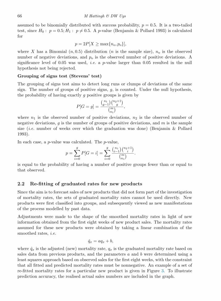
2.2 Re-fitting of graduated rates for new products

Since the aim is to forecast sales of new products that did not form part of the investigationof mortality rates, the sets of graduated mortality rates cannot be used directly. Newproducts were first classified into groups, and subsequently viewed as new manifestationsof the process modelled by past data.

Adjustments were made to the shape of the smoothed mortality rates in light of newinformation obtained from the first eight weeks of new product sales. The mortality ratesassumed for these new products were obtained by taking a linear combination of thesmoothed rates, i.e.

q̂x = aqx + b,

where q̂x is the adjusted (new) mortality rate, qx is the graduated mortality rate based onsales data from previous products, and the parameters a and b were determined using aleast squares approach based on observed sales for the first eight weeks, with the constraintthat all fitted and predicted mortality rates must be nonnegative. An example of a set ofre-fitted mortality rates for a particular new product is given in Figure 3. To illustrateprediction accuracy, the realised actual sales numbers are included in the graph.


Figure 3: A graph of the re-fitted product mortality rates.

2.3 Obtaining forecasts from estimated mortality rates

An estimate of the product’s remaining number of weeks on shelves is obtained by calcu-lating the number of products expected to remain after each week by `x+t = `x×ptx, where`x is the number of products expected to remain after x weeks, and ptx is the probabilityof survival up to week x+ t, given survival up to week x. This can be computed directlyfrom the estimated mortality rates: ptx = (1 − qx)(1 − qx+1) · · · (1 − qx+t). The estimateof the complete future shelf life is equal to the smallest value of t for which `x+t is smallerthan 1% of the initial inventory level.

3 Empirical results

A comparison of the actual vs. predicted shelf life of all three forecasting methods is givenin Figure 4.

The predictions arising from both the forward cover methodology and time series analysisare underestimated, since forecasts are unanimously below the actual values. The survivalanalysis predictions seem to be the most accurate, and are not consistently biased. Toformalise this conclusion, a comparison between the prediction errors and resulting meansquared error (MSE) for each of the models is given below in Table 1.

3.1 Signs test

Resulting p-values for each group is given below in Table 2. Since all p-values are greaterthan 0.1, the null hypothesis for each cohort is not rejected at the 10% significance level.There is thus no significant bias, and the graduation fits the data adequately.

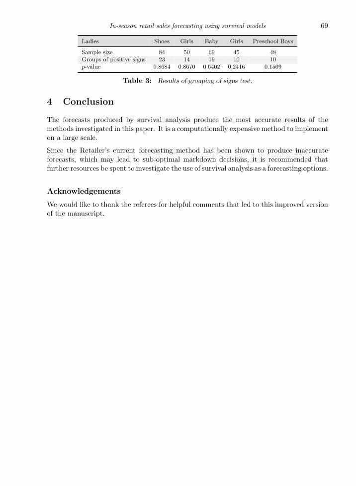
3.2 Grouping of signs test

A summary of results of the grouping of signs test is given in Table 3. Since all p-valuesare greater than 0.1, the null hypothesis is not rejected at the 10% significance level, andit can be concluded that the graduation fits the data adequately.


Figure 4: A plot of the actual vs. predicted number of remaining weeks for the three models.

Prediction errorsForward Time series Survival

Product cover method analysis method

Ladies’ pencil skirt −42 −38 −5Ladies’ bengaline pants −48 −28 3Ladies’ slippers (style A) −4 −2 1Ladies’ slippers (style B) −15 −5 −3Ladies’ slippers (style C) −26 −18 1Girls’ T-shirt (style A) −46 −33 −1Girls’ T-shirt (style B) −7 1 1Baby girls’ fancy top −17 −1 13Baby girls’ leggings −37 −20 1Preschool boys’ yarn dye T-shirt −27 −21 −4Preschool boys’ printed T-shirt −20 −8 1MSE 903.4 416.1 21.3

Table 1: Prediction errors and resulting MSE for the three forecasting methods.

Ladies Shoes Girls Baby Girls Preschool Boys

Sample size 84 50 69 45 48Number of positive deviations 49 21 35 21 21Proportion of positive deviations 58.3% 42.0% 50.7% 46.7% 43.8%p-value 0.101 0.161 0.810 0.766 0.471

Table 2: Prediction errors and resulting MSE for the three survival analysis.

A comparison of the three methods is given in Table 4.


Ladies Shoes Girls Baby Girls Preschool Boys

Sample size 84 50 69 45 48Groups of positive signs 23 14 19 10 10p-value 0.8684 0.8670 0.6402 0.2416 0.1509

Table 3: Results of grouping of signs test.

4 Conclusion

The forecasts produced by survival analysis produce the most accurate results of themethods investigated in this paper. It is a computationally expensive method to implementon a large scale.

Since the Retailer’s current forecasting method has been shown to produce inaccurateforecasts, which may lead to sub-optimal markdown decisions, it is recommended thatfurther resources be spent to investigate the use of survival analysis as a forecasting options.

Acknowledgements

We would like to thank the referees for helpful comments that led to this improved versionof the manuscript.


Meth

od

Facto

rsth

at

fun

dam

enta

llyim

ped

eaccu

racy

of

the

meth

od

Ad

vanta

ges

Disa

dvanta

ges

Forw

ard

cover

meth

od

(Reta

iler’scu

rrent

meth

od

)•

Inap

pro

pria

teto

assu

me

con

stant

sales

over

the

entire

shelf

lifeof

the

pro

du

ct,sin

cep

ast

data

con

firm

sth

at

sales

usu

ally

pea

kd

urin

gth

efi

rst3–5

week

s,an

dth

end

ecrease

as

the

pro

du

ctages.

•V

erysen

sitive

toou

tliersin

the

first

week

sof

sales.

Th

isis

of

particu

lar

con

cern,

since

sales

volu

mes

are

usu

ally

hig

hly

vola

tileth

rou

gh

ou

tth

esea

son

.

•S

heer

simp

licity

•E

ase

of

un

dersta

nd

ing

the

meth

od

•E

ase

of

calcu

latio

n

•F

ull

au

tom

atio

nof

calcu

latio

np

ossib

le

•S

how

nto

be

histo

ri-ca

llyin

accu

rate

(neg

a-

tively

bia

sed)

•A

con

sequ

ence

of

the

ab

ove

isth

at

mark

-d

ow

ns

usu

ally

occu

rto

ola

te,w

ithad

verse

effect

on

reven

ues.

Tim

eseris

an

aly

sis

•In

form

atio

non

the

usu

al

distrib

utio

nof

sales

isavaila

ble

thro

ugh

histo

rical

sales

data

,b

ut

isn

ot

seenby

the

mod

el,w

hich

uses

on

lyd

ata

from

the

first

8w

eeks

of

sales

of

the

new

pro

d-

uct.

•Q

uick

lyan

dea

silyap

plied

•A

mp

leso

ftware

tools

(e.g.S

AS

,S

tatistica

)availa

ble

toen

ab

leau

tom

atio

nof

calcu

latio

n

•S

ign

ifica

nt

level

of

ad

ded

com

plex

ityfo

rlittle

imp

rovem

ent

inaccu

racy

•R

equ

iresso

me

level

of

exp

ertiseto

ap

ply

the

meth

od

Su

rviv

al

an

aly

sis

•T

he

mod

eld

oes

not

take

seaso

nal

facto

rsin

toacco

unt,

e.g.la

rge

sales

volu

mes

over

the

fes-tiv

esea

son

.

•O

ther

extern

al

facto

rs(e.g.

com

petito

rs’ac-

tion

s;co

msu

mer

beh

avio

ur)

are

also

not

taken

into

acco

unt

by

the

mod

el.T

hese

facto

rssh

ou

ldn

everth

elessfo

rmp

art

of

the

mark

dow

nd

ecision

pro

cessin

aqu

alita

tive

sense.

•V

ast

imp

rovem

ent

inaccu

racy

over

forw

ard

cover

meth

od

.

•U

sesh

istorica

lsa

lesd

ata

,w

herea

sth

eoth

erm

ethod

son

lyu

sed

ata

from

the

new

pro

du

ctb

eing

an

aly

sed.

Th

isim

plies

that

the

accu

racy

of

meth

od

may

be

imp

roved

even

furth

erif

more

data

were

used

(inth

isstu

dy,

on

lya

small

sub

setof

the

Reta

iler’sd

ata

was

used

).

•A

pp

licatio

nof

the

meth

od

istim

eco

n-

sum

ing

an

dm

ay

be

diffi

cult

toim

plem

ent

on

ala

rge

scale

(how

-ev

er,so

ftware

tools

cou

ldb

ed

evelo

ped

inord

erto

overco

me

this

pro

blem

).

Tab

le4:

Acom

pariso

nof

the

three

meth

od

su

sedin

this

stud

y.


References

[1] Benjamin B & Pollard JH, 1993, The analysis of mortality and other actuarial statistics, 3rd

Edition, The Institute of Actuaries and The Faculty of Actuaries, London.

[2] Berry MJA, 2009, The application of survival analysis to customer-centric forecasting, Proceedingsof the 22nd Annual NorthEast SAS User Group Conference, Burlington (VI), pp. 1–10.

[3] Broffitt JD, 1984, Maximum likelihood alternatives to actuarial estimators of mortality rates, Trans-actions of Society of Actuaries, 36(1), pp. 77–142.

[4] Chase RB, Jacobs FR & Aquilano NJ, 2006, Operations management for competitive advantage,11th Edition, McGraw-Hill, Monterey (CA).

[5] Chatwin RE, 2000, Optimal dynamic pricing of perishable products with stochastic demand and afinite set of prices, European Journal of Operational Research, 125(1), pp. 149–174.

[6] Cox DR & Oakes D, 1984, Analysis of survival data, Chapman and Hall, London.

[7] Gallego G & Van Ryzin GJ, 1994, Optimal dynamic pricing of inventories with stochastic demandover finite horizon, Management Science, 40(8), pp. 999–1020.

[8] Kincaid WM & Darling DA, 1963, An inventory pricing problem, Journal of Mathematical Analysisand Applications, 7(2), pp. 183–208.

[9] Lobel R & Perakis G, 2013, Dynamic Pricing through sampling based optimisation, [Online], [Cited:14 December 2013], Available from http://ssrn.com/abstract=1748426.

[10] Meckin D, 2007, Naked finance: Business finance pure and simple, Nicholas Brealey Publishing,London.

[11] Mantrala MK & Rao S, 2001, A decision-support system that helps retailers decide order quantitiesand markdowns for fashion goods, Interfaces, 31(3), pp. 146–165.

http://ssrn.com/abstract=1748426

in-season retail sales forecasting using survival models

Documents