In Search of a Factor Model for Optionable Stocks∗

Turan G. Bali† Scott Murray‡

February 2021

Abstract

We propose the first factor model that explains cross-sectional variation in optionable stockreturns. Our model includes new factors based on option-implied volatility minus realizedvolatility, the call minus put implied volatility spread, and the difference between changes incall and put implied volatilities. The model outperforms previously-proposed factor models atexplaining the performance of portfolios of optionable stocks formed by sorting on other option-based predictors, as well as other well-known stock return predictors. The predictive power ofthe option-based factors is driven by informed trading and their exposures to aggregate volatilityand financial uncertainty.

Keywords: Optionable stocks, factor model, cross section of stock returns.JEL Classifications: G11, G12, G13.

∗We thank Adrian Buss, Jie Cao, Tarun Chordia, Zhi Da, Ozgur Demirtas, Stephen Figlewski, Amit Goyal,Bing Han, Cam Harvey, Andrew Karolyi, Jianan Liu, Yukun Liu, David McLean, Quan Wen, Jianfeng Yu, andYu Yuan for insightful comments that have substantially improved the paper. We also benefited from discussionswith seminar participants at Georgetown University and Sabanci University, the 2020 Asia-Pacific Association ofDerivatives Conference, the 2020 International Conference on Derivatives and Capital Markets, the 2020 Conference onthe Theories and Practices of Securities and Financial Markets, the 2021 Bernstein Quantitative Finance Conference,and the 2021 ITAM Finance Conference. Winner of the prize for best paper at the 2020 Asia-Pacific Associationof Derivatives Conference. This work used the Extreme Science and Engineering Discovery Environment (XSEDE),which is supported by National Science Foundation grant number ACI-1548562 (Towns et al. (2014)).†Robert S. Parker Chair Professor of Finance, McDonough School of Business, Georgetown University, tu-

ran.bali@georgetown.edu.‡Assistant Professor of Finance, J. Mack Robinson College of Business, Georgia State University, smur-

ray19@gsu.edu.

1 Introduction

Research investigating the drivers of expected stock returns has documented a large number of

variables that have the ability to predict the cross section of future stock returns.1 Several recent

papers (e.g., Fama and French (2015) and Hou, Xue, and Zhang (2015)) put forth empirical factor

models that are successful at explaining the average returns of most portfolios formed by sorting on

these return predictors. While these papers examine the ability of their models to capture patterns

in average returns associated with a large number of variables calculated from historical stock

market and accounting data, they do not examine the ability of their models to explain anomalies

related to variables calculated from stock option prices (option-based variables hereafter). One

potential reason for the omission of option-based variables from previous studies is that these

variables are only available for optionable stocks, whereas most studies testing the efficacy of a

factor model examine the entire cross section of US common stocks. While historically only 25%

to 75% of all stocks are optionable, these stocks account for between 85% and 98% of total stock

market capitalization, and tend to be more liquid than non-optionable stocks. These facts suggest

that it is important for a factor model to explain predictable patterns in average excess returns

among optionable stocks.

The objective of this paper is to put forth a factor model capable of explaining cross-sectional

variation in average returns of portfolios of optionable stocks. Specifically, we aim to produce the

simplest factor model that explains the returns of portfolios of optionable stocks formed by sorting

on option-based variables and other known predictors of cross-sectional variation in future stock

returns (traditional asset pricing variables hereafter).

The theoretical prediction that a single factor model should price all securities may seem con-

tradictory to our objective of creating a factor model for optionable stocks. However, ever since

Fama and French (1993), who find significant covariation between bond and stock returns but

nonetheless propose different factor models for each type of security, the literature has embraced

the practice of using different empirical factor models for different types of assets.2 Nonetheless, for

1Hou, Xue, and Zhang (2015, 2020), Harvey, Liu, and Zhu (2016), McLean and Pontiff (2016), and Green, Hand,and Zhang (2017) list and categorize many of these predictors.

2Fama and French (1993) propose using a two-factor model with term and default factors for empirical analysesof bond returns, and a three-factor model with the stock market factor, a size factor, and a value factor for empiricalanalyses of stock returns. Lustig, Roussanov, and Verdelhan (2011), Szymanowska, De Roon, Nijman, and VanDen Goorbergh (2014), Bai, Bali, and Wen (2019), and Liu and Tsyvinski (2019) and Liu, Tsyvinski, and Wu (2020)

1

the reader who is uncomfortable with the idea of using different factor models for different subsets

of stocks, an alternative interpretation of our objective is that we aim to create a factor model that

spans the dimensions of stock return predictability arising from known option-based stock return

predictors. This model can serve both as a benchmark for evaluating whether the predictive power

of option-based variables proposed by future research is spanned by previously-known predictors,

and also as a benchmark for assessing whether the predictive power of variables applicable to the

broader set of all stocks is spanned by option-based predictors.

There are at least three reasons that a factor model for optionable stocks is needed. First,

as we will show, previously-proposed factor models, including those that can explain the returns

associated with a large number of anomaly variables, do not explain the returns of portfolios formed

by sorting on option-based variables. While option-based variables are only available for optionable

stocks, this set of predictors is important because the options market is the main venue, other than

the stock market, in which investors can trade based on information or beliefs related to individual

stocks. Insofar as informed trading affects option prices, variables based on option prices are likely to

capture this information. Second, because the OptionMetrics data used by most studies examining

the ability of option-based variables to predict the cross section of future stock returns begin in

1996, the length of the period for which these data are available is becoming more conducive for

this type of research. A factor model that captures the previously-established predictive power of

option-based variables serves as a baseline for ensuring that return predictability documented by

subsequent studies is distinct from these previously-known effects. Third, the universe of optionable

stocks differs substantially from the universe of all stocks in that optionable stocks tend to be larger

and more liquid than other stocks. Factor models aimed at explaining variation in average returns

in the cross section of all stocks may not capture cross-sectional variation in average optionable

stock returns.

Our study focuses on seven previously-established option-based stock return predictors. We

focus on these seven variables because their predictive power among optionable stocks is established

by previous work. Bali and Hovakimian (2009) show that the cross section of future stock returns is

positively related to the difference between option-implied volatility and historical realized volatility

(IV − RV ) and to the difference between the implied volatilities of near-the-money call and put

develop factor models for the currency, commodity, corporate bond, and cryptocurrency markets, respectively.

2

options (CIV −PIV ). Cremers and Weinbaum (2010) find that stocks with high volatility spreads,

measured as the difference between call-implied volatilities and expiration- and strike-matched

put-implied volatilities (V S), have relatively high future returns. Xing, Zhang, and Zhao (2010)

demonstrate that the difference between the implied volatility of an at-the-money (ATM hereafter)

call option and an out-of-the-money (OTM hereafter) put option (Skew), a measure of skewness, is

positively related to the cross section of future stock returns. Johnson and So (2012) find a positive

relation between the ratio of trading volume in the stock to option trading volume (S/O) and future

stock returns. An, Ang, Bali, and Cakici (2014) show that the difference between changes in ATM

call-implied volatility and changes in ATM put-implied volatility (∆CIV − ∆PIV ) is positively

related to future stock returns. Finally, Baltussen, Van Bekkum, and Van Der Grient (2018) find

that the volatility of implied volatility has a negative cross-sectional relation with future stock

returns.3

We begin by examining the ability of our focal variables to predict the cross section of future

stock returns. Our analyses demonstrate that for five of the seven option-based variables, IV −RV ,

CIV − PIV , V S, Skew, and ∆CIV −∆PIV , a value-weighted portfolio that is long stocks with

high values of the variable and short stocks with low values of the variable generates an economically

large and highly statistically significant average excess return. This holds not only during the full

1996-2017 sample period covered by our study, but also in the portion of this period subsequent to

the sample period used in the original study. The persistence of the predictive power of these five

variables after the original studies’ sample periods indicates that these effects are not a result of

data-snooping or publication bias (Harvey, Liu, and Zhu (2016) and Harvey and Liu (2021)) and

do not represent short-lived mispricing that is easily corrected once publicized (McLean and Pontiff

(2016)). As such, any factor model for optionable stocks must be able to account for these pricing

effects.

Next, we use the Fama and French (1993) methodology to generate factor portfolios associated

with each of the five variables with strong predictive power: IV −RV , CIV −PIV , V S, Skew, and

∆CIV −∆PIV (option-based factors hereafter). We then search for the smallest subset of these five

3In their expositions, many of the papers find a negative relation between their variables and future stock returns.So that all of our focal variables have a positive cross-sectional relation with future stock returns, for variablesdocumented to have a negative relation with future returns, we define our versions of these variables as the negativeor inverse of the versions used in the original papers.

3

option-based factors that, when combined with the market factor (MKT ), produces a factor model

that explains the average returns of all five of the option-based factors. We find that a factor model

that includes MKT and factors based on IV − RV (FIV−RV ), V S (FV S), and ∆CIV − ∆PIV

(F∆CIV−∆PIV ) explains the average returns of all of the option-based factors. No other model that

combines MKT with three or fewer option-based factors satisfies this criterion. We therefore settle

on a model that includes MKT , FIV−RV , FV S , and F∆CIV−∆PIV as our benchmark model.4

The fact that fewer than five option-based factors are needed to explain the average returns

of all five factors is not unexpected. The original papers examining these variables argue that

many of the option-based variables capture the trading of informed investors. As described in

Easley, O’Hara, and Srinivas (1998), informed investors may chose to trade in the options market.

Insofar as informed investors have positive (negative) information about a stock, they will buy

(sell) calls and sell (buy) puts, and this demand will have an impact on option prices (Bollen

and Whaley (2004), Garleanu, Pedersen, and Poteshman (2009)), causing the implied volatility

of calls (puts) to be higher than that of puts (calls). Furthermore, CIV − PIV , Skew, V S, and

∆CIV − ∆PIV all capture differences between the implied volatility of calls and that of puts.

Given the similarities between the option-based measures, it is not surprising that a model that

includes only three option-based factors explains the average returns of all five factors. The fact that

we cannot explain the average excess returns of all five factors with fewer than three non-market

factors indicates that the measures underlying each of these factors captures a distinct dimension

of stock return predictability.

To test our model, we investigate its ability to explain the average returns generated by portfo-

lios of optionable stocks formed by sorting on option-based variables and traditional asset pricing

variables. Not surprisingly given the methodology we use to select the factors included in our

model, we find that our four-factor model explains the average returns of portfolios formed by

sorting on each of the option-based variables. More importantly, we find that portfolios of option-

able stocks formed by sorting on most of the traditional asset pricing anomaly variables studied

4Recent studies have shown that machine learning models are capable of generating robust predictions of futurestock returns from a large number of input variables in a manner that addresses data-snooping concerns, and identi-fying the marginal contribution of new factors relative to the large set of existing ones (Feng, Giglio, and Xiu (2020),Gu, Kelly, and Xiu (2020), Kozak, Nagel, and Santosh (2020), and Giglio, Liao, and Xiu (2021)). The small set ofoption-based variables shown by the prior work to predict future stock returns enables us to achieve these objectiveswithout the use of these modern techniques.

4

by Stambaugh, Yu, and Yuan (2012, 2014, 2015) and Green, Hand, and Zhang (2017) generate

insignificant alphas relative to our four-factor model. We also find that the Sharpe ratio of the

tangency portfolio constructed from the factors in our model is significantly higher than that of

previously-established factor models. Our last tests of our model show that the performance of

optionable stock versions of most factors in previously-proposed factor models is explained by our

model. However, augmenting our model with an optionable stock-based profitability factor may

enable the model to capture additional dimensions of return predictability.

Finally, we investigate the economic channels that drive the performance of the option-based

factors in our model. We find that our model explains the performance of portfolios sorted on

exposure to aggregate volatility, which indicates that a component of the performance of our factors

is related to aggregate volatility risk. We also find that our factors perform better following periods

of high aggregate uncertainty, suggesting that financial market uncertainty plays an important role

in the performance of our factors. Lastly, we find that the predictive power of the option-based

variables underlying our factors is stronger among stocks with low-institutional ownership than

among stocks with high-institutional ownership, indicating that the option-based variables capture

informed trading in the options market.

The remainder of this paper proceeds as follows. In Section 2 we contextualize our contributions

in the extant literature. Section 3 describes our sample and demonstrates the predictive power of

previously-studied option-based variables. In Section 4 we construct our option-based factors and

select the factors to be included in our model. Section 5 demonstrates that our four-factor model

does a better job than previously-proposed factor models at explaining the average returns of

portfolios of optionable stocks. Section 6 investigates the economic channels underlying the factors

in our model. Section 7 concludes.

2 Literature Review

Our work contributes directly to two main lines of research. First, we add to the work that aims to

produce empirically-motivated factor models that explain cross-sectional variation in average stock

returns. The seminal paper in this area is Fama and French (1993), who pioneered the methodology

most commonly used for generating factor portfolios and whose three-factor model (FF model

5

hereafter) that includes a market factor, a size factor, and a value factor, was the standard for many

years. Carhart (1997) proposed a four-factor model (FFC model hereafter) that augments the FF

model with a momentum factor designed to capture variation in average returns associated with

the momentum effect of Jegadeesh and Titman (1993). Pastor and Stambaugh (2003) developed

an aggregate liquidity factor that led many researchers to adopt a five-factor model (FFCPS model

hereafter) that included the four factors in the FFC model and the aggregate liquidity factor.

Subsequent to this, the large proliferation in documented anomalies led to the proposal of several

alternative factor models designed to capture return variation common to several pricing effects.

Fama and French (2015) propose a five-factor model (FF5 model hereafter) that includes a market

factor, a size factor, a value factor, an investment factor, and a profitability factor. Hou et al. (2015)

propose a four-factor model (Q model hereafter) that includes the market factor, a size factor, an

investment factor, and a profitability factor. The objective of all of these previous papers is to

explain anomalies based on variables constructed from accounting and historical stock market data

that are present in the entire cross section of US common stocks. Our objective differs from that

of previous work in that we focus only on optionable stocks. To our knowledge, our factor model

is the first to be able to explain cross-sectional variation in returns associated with option-based

variables.

Second, we contribute to the line of research that examines the ability of option-based variables

to predict the cross section of future stock returns. In addition to the papers, discussed above, that

originally document the effects that we focus on, Pan and Poteshman (2006) find that, when looking

only at volume initiated by buyers to open new positions, the ratio of put to call option volume

is negatively related to the cross section of future stock returns. We do not investigate this effect

because calculation of the focal measure used by Pan and Poteshman (2006) requires proprietary

data that are not available publicly. As discussed by Pan and Poteshman (2006), the ratio of put

to call option volume for all trades, which can be calculated from publicly-available data, has no

ability to predict the cross section of future stock returns. Conrad, Dittmar, and Ghysels (2013)

demonstrate that average historical option-implied skewness is negatively related to the cross section

of future stock returns.5 We do not investigate their measure because the data requirements for

5Amaya, Christoffersen, Jacobs, and Vasquez (2015) find similar results using a measure of skewness generatedfrom high-frequency stock return data.

6

calculating this measure are only satisfied by a small proportion of optionable stocks. Consistent

with Xing et al. (2010), Rehman and Vilkov (2012) and Chordia, Lin, and Xiang (2020) find that

risk-neutral skewness positively predicts the cross-section of stock returns, a result that Chordia

et al. (2020) attribute to informed trading. We contribute to this line of work by showing that the

predictive power of a large number of these option-based predictors is captured by a factor model

that includes only four factors, one of which is the market factor. Our results indicate that while

most of these measures robustly predict the cross section of future stock returns, the predictive

power of some measures is redundant. We are also the first paper to simultaneously examine the

predictive power of option-based and traditional asset pricing variables. Most importantly, we

provide a factor model to be used as a benchmark by future research examining relations between

option-based variables and the cross section of average stock returns.

More broadly, our work is related to several other lines of work. Many papers have used

option-based measures to predict the returns of securities other than stocks. Among these are Cao,

Goyal, Xiao, and Zhan (2020b), who find that changes in option-implied volatility predict the cross

section of future corporate bond returns, and Driessen, Maenhout, and Vilkov (2009), Goyal and

Saretto (2009), Vasquez (2017), and Hu and Jacobs (2020), who detect relations between predictors

generated from option prices and the cross section of future option returns.6 Other papers, such

as Ang et al. (2006), Chang, Christoffersen, and Jacobs (2013), Cremers, Halling, and Weinbaum

(2015), and Lu and Murray (2019), detect relations between expected stock returns and exposure

to factors from S&P 500 index options prices. Exposure to index option return-based factors has

also been shown by Fung and Hsieh (2001), Agarwal and Naik (2004), and Jurek and Stafford

(2015) to explain variation in hedge fund returns.

Finally, a large number of papers have used option-based variables in other asset pricing con-

texts. An incomplete list of such papers is as follows. Roll, Schwartz, and Subrahmanyam (2010)

find a contemporaneous (but not predictive) relation between option trading volume and stock

returns. DeMiguel, Plyakha, Uppal, and Vilkov (2013) show that incorporating information from

option prices when constructing portfolios can help decrease portfolio volatility and increase the

portfolio’s Sharpe ratio. Buss and Vilkov (2012) and Chang, Christoffersen, Jacobs, and Vainberg

6Cao and Han (2013) find that idiosyncratic volatility measured from stock returns predicts the cross-section offuture option returns. Cao, Han, Tong, and Zhan (2020c) demonstrate that several variables known to predict thecross section of future stock returns also predict the cross section of delta-hedged option returns.

7

(2012) generate forward-looking measures of risk from option data. Cao, Goyal, Ke, and Zhan

(2020a) find that the price informativeness of a stock increases when options on the stock are first

listed.

3 Data, Variables, and Sample

Option data are from OptionMetrics (OM hereafter). We use OM’s traded options data and OM’s

implied volatility surface. The traded options data include the daily end-of-day best bid, best

ask, implied volatility, and Greeks for options traded on the Chicago Board Options Exchange.

To ensure data quality, we keep only observations with a positive best bid price, a best offer

price that is greater than the best bid price, a positive implied volatility, which indicates that

the option price does not violate simple no-arbitrage conditions, positive open interest, and whose

bid-ask spread scaled by the mid price is less than 0.5. The volatility surface data contain implied

volatilities for options with fixed times to expiration and deltas constructed using interpolation.

Stock price, return, volume, and shares outstanding data are from CRSP. Accounting data are

from COMPUSTAT. We gather daily and monthly returns for the market, size, and value factors

of Fama and French (1993), a momentum factor, the size, value, investment, and profitability

factors of Fama and French (2015), and the risk-free asset from Ken French’s data library.7 We

collect the returns of the Pastor and Stambaugh (2003) traded liquidity factor from Lubos Pastor’s

website.8 The market, size, investment, and profitability factors of Hou et al. (2015) are obtained

from their online data library.9

3.1 Variables

To the extent possible, we calculate the option-based variables in the same manner as in the original

studies of these variables. Since these variables are well-established in the literature, we provide

a brief description of their calculation here, and relegate detailed descriptions to Appendix A. All

variables are calculated at the end of each month for all stocks for which the data requisite for the

calculation of the given variable are available.

7Ken French’s data library is at https://mba.tuck.dartmouth.edu/pages/faculty/ken.french/data library.html.8Lubos Pastor’s website is http://faculty.chicagobooth.edu/lubos.pastor/research/.9http://global-q.org/index.html

8

IV −RV and CIV −PIV are calculated following Bali and Hovakimian (2009) as the difference

between ATM option-implied and historical realized volatility, and the difference between ATM call-

implied volatility and ATM put-implied volatility, respectively. V S is calculated following Cremers

and Weinbaum (2010) as the weighted-average difference between strike- and maturity-matched call-

implied and put-implied volatilities, with weights determined by open interest. Skew is calculated

following Xing et al. (2010) as the implied volatility of an ATM call minus the implied volatility of

an OTM put. S/O is calculated following Johnson and So (2012) as stock trading volume divided

by option trading volume. Since Johnson and So (2012) focus on weekly returns and our study

focuses on monthly returns, we make reasonable modifications of their variable to accommodate

our monthly frequency. ∆CIV −∆PIV is calculated following An et al. (2014) as the one-month

change in ATM call-implied volatility minus the one-month change in ATM put-implied volatility.

Finally, volatility of implied volatility (V oV ) is calculated following Baltussen et al. (2018) as the

negative of the standard deviation of the daily implied volatility of the stock’s ATM options over

the past month, scaled by the mean of the implied volatilities. Following the original papers, the

calculation of IV − RV , CIV − PIV , V S, Skew, S/O, and V oV uses OM’s traded option data,

and the calculation of ∆CIV −∆PIV uses data from OM’s implied volatility surface.

The original studies of IV − RV , Skew, ∆CIV − ∆PIV , and V oV actually use RV − IV ,

−Skew, ∆PIV −∆CIV , and −V oV , the negative of our variables, and find negative cross-sectional

relations between their variables and future stock returns. Similarly, Johnson and So (2012) use

the ratio of option to stock volume (O/S) and find a negative relation between that and future

stock returns. We use the negative or inverse of these variables so that all of our variables have a

positive relation with future stock returns. Throughout this paper, all volatilities used to calculate

IV −RV , CIV − PIV , V S, Skew, ∆CIV −∆PIV , and V oV are recorded in percent. Thus, for

example, if IV − RV has a value of 1.00, this indicates that the implied volatility of the stock is

one percentage point higher than the stock’s realized volatility.

3.2 Sample

Our sample consists of all optionable US-based common stocks that trade on the NYSE, AMEX,

or NASDAQ (optionable stocks hereafter) and covers the 1996-2017 period for which OM data are

9

available.10 Specifically, the sample created at the end of each month t, which will be used to

examine the cross-sectional relation between variables calculated at the end of month t and stock

returns in month t+ 1, includes each optionable stock that, as of the end of month t, is both a US-

based common stock and trades on either the NYSE, AMEX, or NASDAQ. A stock is considered

optionable if, on the last trading day of month t, it appears in OM’s traded options data. We also

require that each stock in the month t sample has a non-missing price and positive number of shares

outstanding at the end of month t. Our sample includes the 263 sample formation months t (future

return months t + 1) from February (March) 1996 through December 2017 (January 2018). Our

first sample formation month t is February 1996, instead of January 1996, because ∆CIV −∆PIV ,

one of our focal variables, requires data from both months t and t− 1, making February 1996 the

first month for which this measure is available.

Table 1, Panel A presents summary statistics for the focal variables used in our study. Each

month t, we calculate the cross-sectional mean, standard deviation, and median value of each

variable, as well as the number of stocks for which the variable can be calculated. The table presents

the time-series means of the monthly cross-sectional summary statistics. IV −RV is positive in both

mean and median, indicating that implied volatilities tend to be higher than realized volatilities.

Both CIV − PIV and V S have a negative mean and median, indicating that both the average

and majority of stocks have higher put implied volatilities than call implied volatilities. Skew is,

on average and in median, negative, indicating that ATM call implied volatilities tend to be lower

than OTM put implied volatilities. S/O is 96.58 (46.93) on average (in median), indicating that

stock trading volume is much higher than option trading volume. ∆CIV −∆PIV is close to zero in

both mean and median, indicating that neither call implied volatilities nor put implied volatilities

have a tendency to increase more than the other. Finally, V oV has a mean (median) of −7.84

(−6.86), indicating that for the mean (median) stock, the daily variation in implied volatility is

approximately 8% (7%) of the level of implied volatility.

The time-series averages of monthly cross-sectional correlations between the variables are shown

in Panel B of Table 1. The results indicate that pairwise correlations between CIV − PIV , V S,

Skew, and ∆CIV −∆PIV are all strongly positive. This is not surprising because each of these

10US-based common stocks are taken to be stocks with CRSP share code (shrcd field) value of 10 or 11. Stockswith CRSP exchange code (exchcd field) value of 1, 2, or 3 are taken to trade on the NYSE, AMEX, and NASDAQ,respectively.

10

variables, in some way, captures the difference between the implied volatility of calls and the implied

volatility of puts. V oV has a modest positive correlation with each of IV − RV and S/O. Aside

from this, IV −RV , V oV , and S/O each have near-zero correlations with all of the other variables.

To compare the sample of optionable stocks to that of all US-based common stocks listed on

the NYSE, AMEX, and NASDAQ (all stocks hereafter), in Table 2 we present summary statis-

tics for market capitalization (MktCapShareClass), illiquidity (Illiq), Price (Price), share volume

(V olume), and dollar trading volume (V olume$) for both optionable stocks and the sample of all

stocks. MktCapShareClass for stock i in month t is measured as the share price times the number

of shares outstanding of the stock, as of the end of month t, recorded in millions of US dollars. We

include the subscript ShareClass on MktCapShareClass to stress that this variable is measured at

the share class level, and not aggregated across share classes to the firm level. This distinction is

notable here because for firms with multiple share classes, some share classes may be optionable

and others may not be. Illiq for stock i in month t is calculated following Amihud (2002) as the

average, over all days in months t− 11 through t, inclusive, of the absolute daily return (mesaured

in percent) divided by dollar trading volume (measured in millions of US dollars). Price is the

price of the stock at the end of the month. V olume is the number of shares of the stock traded

in the given month, recorded in thousands of shares. V olume$ is the dollar trading volume of the

stock, calculated as V olume× Price/1000, and thus is recorded in millions of dollars. The month

t sample of all stocks is constructed in exactly the same way as our focal sample, except we do not

require a stock to be optionable for it to enter the sample of all stocks.

Table 2 demonstrates that there are substantial differences between the sample of optionable

stocks that we focus on in this paper and the broader sample of all US-based common stocks. In the

average month, a little less than half of all stocks are optionable, the median market capitalization

of optionable stocks is more than 3.5 times that of all stocks, and the median value of Illiq for

optionable stocks of 0.31 is less than one 20th that of all stocks. The price of the median optionable

stock is $23.04 and that of all stocks is $14.52. Share volume (dollar trading volume) of optionable

stocks is, in median, a little more than three (five) times that of all stocks. The results clearly

demonstrate that optionable stocks tend to be larger and more liquid than stocks in the broader

sample of US-based common stocks. Interestingly, due to a small number of stocks that are not

optionable but have very high prices, the mean price of optionable stocks is substantially lower

11

than the mean price of all stocks.

We continue our comparison of the optionable stock sample and all stocks sample by construct-

ing time-series plots of the number of stocks, the total market capitalization of the stocks, and the

total dollar trading volume of the stocks in each sample. Figure 1 plots the number of all stocks as

well as the number of stocks that are optionable, through time. The figure shows that at the end

of February 1996 (the beginning of our sample period), only 1,574 of the 6,982, or about 22.5%

of all stocks were optionable. However, by the end of our sample period in December 2017, 2,650

out of 3,605 such stocks (73.5%) were optionable. Interestingly, the increase in the percentage of

all stocks that are optionable is as much a manifestation of a decrease in the total number of all

stocks as it is of an increase in the number of optionable stocks.

Figures 2 and 3 show the total market capitalization and total monthly dollar trading volume

for both all stocks and optionable stocks. Despite the fact that the maximum percentage of stocks

that are optionable is 75.9% (in August 2016), the percentage of total market capitalization (dollar

trading volume) for all stocks that comes from optionable stocks ranges from a minimum of 85.5%

in September 1996 (85.0% in June 1996) to 98.5% in August 2016 (99.7% in March 2016). Thus,

even during the early part of our sample period when most stocks were not optionable, the sample

of optionable stocks accounted for the vast majority of total market capitalization and total dollar

trading volume of all stocks. These results demonstrate the importance of understanding patterns

in the returns of optionable stocks.

3.3 Ability of Option-Based Variables to Predict Future Returns

Our first asset pricing tests are portfolio analyses examining the ability of our focal option-based

variables to predict the cross section of future stock returns. At the end of each month t, we group

all optionable stocks into five portfolios based on ascending values of the given variable. The break-

points used to group the stocks are the 20th, 40th, 60th, and 80th percentile values of the variable

among NYSE-listed optionable stocks. We then calculate the month t + 1 MktCapShareClass-

weighted (value-weighted hereafter) average excess return for stocks in each portfolio, as well as

that of a portfolio that is long the fifth quintile portfolio and short the first quintile portfolio in

equal dollar amounts (long-short portfolio hereafter). Our decision to use NYSE breakpoints and

value-weighted portfolios follows Hou et al. (2015, 2020), who find that this methodology provides

12

a more stringent test than using breakpoints based on all stocks or equal-weighted portfolios. This

portfolio construction methodology is also consistent with well-established research practice (Fama

and French (1993, 2015)). In Section I and Tables IA1-IA5 of the Internet Appendix, we show that

our conclusions are unchanged when we examine portfolios constructed using breakpoints calculated

from all optionable stocks.

Table 3 presents the time-series averages of the monthly excess returns for each value-weighted

long-short portfolio, along with a Newey and West (1987)-adjusted t-statistic testing the null hy-

pothesis that the portfolio’s average excess return is zero. The table also presents alphas relative

to a one-factor market model (CAPM model) that includes only the market factor, the FF, FFC,

FFCPS, FF5, and Q factor models, a seven-factor model that augments the FF5 model with the

momentum and liquidity factors (FF5CPS model hereafter), and a six-factor model that adds the

momentum and liquidity factors to the Q model (QCPS model hereafter). The factors in the FF,

FFC, FFCPS, FF5, and Q models are described in Section 2. A portfolio’s alpha with respect to

any given factor model is the estimated intercept coefficient from a time-series regression of the

portfolio’s excess returns on the factors included in the model. All returns and alphas presented

in Table 3 and the remainder of this paper are in percent per month. For example, a value of 1.00

indicates an excess return or alpha of 1.00% per month.

The results of the portfolio analyses for the full March 1996 through January 2018 period are

presented in Panel A of Table 3. The results show that the value-weighted long-short portfolios

formed by sorting on IV −RV , CIV −PIV , V S, Skew, and ∆CIV −∆PIV generate economically

large and highly statistically significant average excess returns during this period, ranging from

0.49% per month (t-statistic = 2.86) for the Skew portfolio to 0.85% per month (t-statistic = 4.25)

for the V S portfolio. For each of these portfolios, the alpha relative to all factor models is positive,

economically large, and highly statistically significant. The results indicate that previously proposed

factor models that have been shown to explain cross-sectional variation in future returns associated

with a large number of predictive variables do not explain the average returns of portfolios formed

by sorting on IV −RV , CIV − PIV , V S, Skew, and ∆CIV −∆PIV .

The long-short portfolio formed by sorting on S/O generates an insignificant average excess

return of 0.29% per month (t-statistic=1.22), significant positive alphas relative to the FFC and

FFCPS models, but insignificant alphas with respect to the other six factor models. There are

13

several potential reasons for the relatively weak predictive power of S/O in our sample. First,

since our sample includes seven years of data (2011-2017) not included in Johnson and So (2012)’s

sample, it is possible that the predictive power of S/O is weak during these years. We examine this

possibility shortly. Second, Johnson and So (2012) use weekly returns and equal-weighted decile

portfolios, whereas we use monthly returns and value-weighted quintile portfolios. It is possible that

these methodological differences account for the weak predictive power of S/O in our analysis.11

Finally, the V oV long-short portfolio produces an average excess return of 0.26% per month

(t-statistic = 1.14). The weak results for this portfolio are a bit more surprising than those for the

S/O portfolio given that the main empirical difference between our analysis and that in Baltussen

et al. (2018) is that our sample period includes the November 2014 through January 2018 period

coming after the sample period in the original study. Our analysis suggests that the V oV effect

may be weak during the November 2014 through January 2018 period, a result we verify shortly.12

Two potential concerns with the results in Panel A of Table 3 are that, because the March

1996 through January 2018 sample period examined in these tests includes the sample period used

in the original studies, the results in Panel A may simply be a manifestation of publication bias

(Harvey et al. (2016)) or are potentially no longer relevant because mispricing was corrected after

the original paper was made public (McLean and Pontiff (2016)).

To address these concerns, in Panel B of Table 3, we present the results of analyses of the

performance of the long-short portfolios during the period subsequent to the sample period used

in the original study.13 The results indicate that the long-short portfolios formed by sorting on

IV −RV , CIV − PIV , V S, Skew, and ∆CIV −∆PIV all continue to generate positive average

excess and risk-adjusted returns in the period subsequent to that used by the original studies

11In unreported results, we find that a monthly long-short portfolio constructed from equal-weighted decile port-folios generates a significantly positive average excess return and alphas with respect to most models during theFebruary 1996-December 2010 period. This suggests that our use of monthly data does not cause our results todiverge from those in Johnson and So (2012). Results in Table 2 of Johnson and So (2012) suggest that a large com-ponent of the S/O effect is driven by the extreme deciles. While Johnson and So (2012) find that their results holdwhen comparing deciles one and two of S/O to deciles nine and ten of S/O, their analysis takes the equal-weightedaverage of deciles one and two, and the same for deciles nine and ten. Our quintile portfolios weight the decilesaccording to the aggregate market cap in each decile.

12In unreported results, we verify that the V oV long-short portfolio generates a positive and statistically significantFF alpha during the February 1996 through October 2014 period examined by Baltussen et al. (2018).

13The original studies using IV − RV , CIV − PIV , V S, Skew, S/O, ∆CIV − ∆PIV , and V oV use sampleperiods ending in portfolio formation (return) months December 2004 (January 2005), December 2004 (January2005), December 2005 (January 2006), December 2005 (January 2006), November 2010 (December 2010), December2011 (January 2012), and September 2014 (October 2014), respectively.

14

of these variables. For IV − RV , CIV − PIV , V S, and Skew, the average returns and alphas

of the long-short portfolios are all economically large and, with a few minor exceptions, highly

statistically significant. The long-short portfolio formed by sorting on ∆CIV −∆PIV generates

a statistically insignificant average monthly excess return of 0.28% (t-statistic = 1.57). However,

the short post-original study period examined by this test, February 2012 through January 2018,

causes this test to have low power. We therefore interpret this result as suggesting that the positive

relation between ∆CIV − ∆PIV and future stock returns persists beyond the period examined

in the original study. The S/O long-short portfolio generates an average excess return of 0.01%

per month (t-statistic = 0.08) during the January 2011 through January 2018 period subsequent

to that used by Johnson and So (2012), suggesting that S/O does not have strong out-of-sample

predictive power. The results for the long-short portfolios formed by sorting on V oV show that this

portfolio generates economically large and statistically significant negative average excess returns

and alphas. Thus, while V oV is positively related to future stock returns during the March 1996

through October 2014 sample period studied by Baltussen et al. (2018), our results indicate a

strong negative relation between V oV and future stock returns during the November 2014 through

January 2018 period.14

From the results in Table 3, we conclude that IV −RV , CIV −PIV , V S, Skew, and ∆CIV −

∆PIV are all positively related to future stock returns in the cross section. There does not appear

to be a robust relation between expected stock returns and S/O or V oV . The analyses in the

remainder of the paper, therefore, use only IV −RV , CIV −PIV , V S, Skew, and ∆CIV −∆PIV

as option-based variables.

4 Option-Based Factors

We proceed now to the main objective of the paper, which is to generate a factor model that

explains the average returns of portfolios of optionable stocks.

14As a robustness check, in Section II and Table IA6 of the Internet Appendix, we demonstrate that our resultsare qualitatively similar when using only the subset of stocks for which all seven option-based predictors can becalculated.

15

4.1 Factor Construction

We begin by creating a factor based on each of IV − RV , CIV − PIV , V S, Skew, and ∆CIV −

∆PIV . The factors are constructed using a methodology similar to that of Fama and French (1993).

At the end of each month t, all optionable stocks are divided into two groups based on firm-level

market capitalization (MktCapFirm) and three groups based on the given option-based variable.

MktCapFirm for stock i is defined as the sum of MktCapShareClass across all share classes for the

firm issuing stock i. The reason for sorting on market capitalization is to make the portfolio largely

neutral to the size effect documented by Fama and French (1992), who show that stocks of firms

with low market equity tend to generate higher returns than stocks of firms with high market equity.

We use MktCapFirm instead of MktCapShareClass when sorting stocks into market capitalization

groups to align our portfolio construction methodology with Fama and French (1993)’s view that

the size effect exists because the stocks of small firms are exposed to priced risks that stocks of

large firms are not exposed to. The MktCapFirm breakpoint is the median MktCapFirm among all

optionable stocks listed on the NYSE. The breakpoints for the option-based variable are the 30th

and 70th percentile values of the given variable among optionable NYSE-listed stocks.

We then sort all optionable stocks into six portfolios using the breakpoints calculated from only

NYSE-listed optionable stocks, and take the month t+ 1 excess return of each portfolio to be the

MktCapShareClass-weighted average excess return of the stocks in the portfolio. Finally, the month

t + 1 factor excess return is defined as the average excess return of the above-median and below-

median MktCapFirm portfolios for the stocks with high values of the given option-based variable

minus that of the above-median and below-median MktCapFirm portfolios for the stocks with low

values of the given option-based variable. We use FX to denote the excess returns of the factor

constructed from the variable X.

Table 4 presents summary statistics for the full March 1996 through January 2018 period

(Panel A), summary statistics for the period subsequent to the sample period used in the original

study of the given option-based variable (Panel B), and correlations for the full sample period

(Panel C) for the excess returns of the option-based factors and the market factor (MKT ). The

summary statistics demonstrate that each factor generates a positive, economically large, and highly

statistically significant average excess return both during the full sample period, and during the

16

period subsequent to that examined in the original study of the option-based variable used to

construct the factor. The correlations show that, as expected based on the correlations between

the stock-level variables (see Table 1, Panel B), FCIV−PIV , FV S , FSkew, and F∆CIV−∆PIV are all

strongly positively correlated. The correlation between each of these factors and MKT is small.

FIV−RV has a moderate positive correlation with FSkew, a negative correlation with MKT , and

close to zero correlation with the other factors.

We next examine whether the option-based factors’ average excess returns can be explained

by previously proposed factor models by examining the alpha of each option-based factor relative

to each of the previously-proposed factor models. The results of these analyses, shown in Table

5, indicate that the CAPM, FF, FFC, FFCPS, FF5, Q, FF5CPS, and QCPS factor models all

fail to explain the positive average excess returns generated by each of the option-based factors.

With one exception, the alpha of each of the option-based factors with respect to each factor model

is positive and highly statistically significant. The one exception is the 0.23% per month alpha

of FSkew relative to the FF5CPS model, which is statistically weak at conventional levels with a

t-statistic of 1.85.

4.2 Option-Based Factor Model

Having demonstrated that previously-established factor models do not explain the average returns

of the option-based factors, we proceed to determining which factors should be included in our

optionable stock factor model. While previously-proposed factor models do not explain the average

returns of the option-based factors, the high correlations between many of the option-based factors

suggest that the returns generated by one or more of these factors may be explained by some

combination of other option-based factors. If this is the case, a factor model that includes only a

subset of the option-based factors may suffice for explaining the cross section of optionable stock

returns. The objective of our factor selection methodology is to find the smallest subset of option-

based factors that spans all dimensions of return predictability captured by the full set of factors.

To determine which option-based factors should be included in our model, we begin by ex-

amining whether the average return generated by each option-based factor can be explained by a

five-factor model that includes MKT and the other four option-based factors. We include MKT

in the factor models because, as discussed in Fama and French (1993), “the market factor is needed

17

to explain why stock returns are on average above the one-month bill rate.” Thus, while the MKT

factor may not be important for explaining the average returns of long-short portfolios such as the

option-based factors, it is likely to be important for explaining the average returns generated by

long-only stock portfolios.

The results of these analyses, presented in Table 6 Panel A, show that the alpha of each of

FIV−RV , FV S , and F∆CIV−∆PIV relative to a factor model that includes MKT and the other

option-based factors is positive and highly statistically significant. This indicates that the average

return generated by each of these factors is not explained by a linear combination of the other

option-based factors. The alphas generated by FCIV−PIV and FSkew, on the other hand, are small

and statistically insignificant, indicating that the average return generated by each of these factors

is captured by a linear combination of other option-based factors and MKT . The slope coefficients

from these regressions indicates that FCIV−PIV loads heavily on FV S and has relatively small but

statistically significant loadings on FSkew and F∆CIV−∆PIV . FSkew loads heavily on FCIV−PIV and

has a small but significant loading on FIV−RV .

Since the average returns generated by FCIV−PIV and FSkew are explained by combinations of

the other option-based factors, we proceed to examine whether a model with only MKT , FIV−RV ,

FV S , and F∆CIV−∆PIV can explain the average returns generated by FCIV−PIV and FSkew. Panel B

of Table 6 shows the results of regressions of each of FCIV−PIV and FSkew on MKT , FIV−RV , FV S ,

and F∆CIV−∆PIV . The results indicate that the four-factor model with MKT , FIV−RV , FV S , and

F∆CIV−∆PIV explains the average returns generated by FCIV−PIV and FSkew. For both FCIV−PIV

and FSkew, the alpha relative to the four-factor model is small and statistically indistinguishable

from zero. In Section III and Table IA7 of the Internet Appendix, we show that the factor model

that includes MKT , FIV−RV , FV S , and F∆CIV−∆PIV is the only model that includes MKT and

three or fewer of the option-based factors that explains the average returns of all of the option-based

factors.

The results in this section suggest that a four-factor model that includes MKT , FIV−RV ,

FV S , and F∆CIV−∆PIV explains the average returns of all of the option-based factors, and that

FCIV−PIV and FSkew are redundant. We therefore propose this four-factor model, which we refer

to as the OPT model, as a benchmark for measuring the abnormal returns generated by portfolios

of optionable stocks.

18

5 Pricing Tests

This section tests the effectiveness of the OPT model on a broad set of optionable stock portfolios

and compares the performance of the OPT model to that of previously-proposed factor models.

5.1 Portfolios Formed by Sorting on Option-Based Variables

The first tests of our OPT model examine whether the model can explain the average returns of

long-short portfolios formed by sorting stocks based on IV − RV , CIV − PIV , V S, Skew, and

∆CIV −∆PIV . The long-short portfolios we examine here are the exact same long-short portfolios

examined in Section 3.3 and Table 3. Table 7 presents the results of factor regressions of long-short

portfolio excess returns on the four factors in the OPT model. The alpha of each of the long-short

portfolios relative to the OPT model is economically small and statistically insignificant, indicating

that our model does a good job at explaining the average returns of these long-short portfolios.

The estimated factor exposures provide some insight into which factors are important for ex-

plaining the average returns generated by the long-short portfolios. We focus our discussion here on

the CIV −PIV and Skew long-short portfolios because these portfolios are constructed from vari-

ables other than those upon which the factors in our model are formed. The CIV −PIV portfolio

has a large and highly significant positive loading on FV S , indicating that this factor is important

for explaining the average return generated by the CIV −PIV portfolios. The CIV −PIV portfolio

also has a significant but economically smaller negative loading of −0.17 on FIV−RV . The Skew

long-short portfolio has a large and highly significant positive loading of 0.60 (t-statistic = 4.56) on

F∆CIV−∆PIV and small and insignificant loadings on all other factors, suggesting that the average

return earned by the Skew long-short portfolio is explained by its exposure to F∆CIV−∆PIV .

To further test whether our factor model captures all dimensions of stock return predictability

arising from the option-based variables, we construct portfolios based on a principal component (PC

hereafter) analysis of the excess returns of the long-short portfolios formed by sorting on IV −RV ,

CIV − PIV , V S, Skew, and ∆CIV −∆PIV . The return of the kth PC portfolio in any month

t is calculated by summing, across all five long-short portfolios, the weight of the given long-short

portfolio in the kth PC times the month-t excess return of the long-short portfolio.15 Panel A

15Section IV and Tables IA8-IA9 of the Internet Appendix present the weights of each long-short portfolio in eachprincipal component portfolio, the amount of the total variance of the principal components that is captured by each

19

of Table 8 shows that the average excess returns of the first three PC portfolios are large and

significant (only marginally so for the third PC), whereas the average excess return of the fourth

and fifth PC portfolios are small and insignificant. The alphas of all five PC portfolios with respect

to our four-factor OPT model are small and insignificant. Panel B shows that, when subjected to

established factor models, the first three PC portfolios all generate economically substantial and,

with the exception of the third PC portfolio for some models, highly significant alphas, whereas

the alphas of the fourth and fifth PC portfolios are all small and insignificant. Taken together, the

results confirm our finding that only three factors are needed to span the return predictability of all

of the option-based variables, and that these dimensions of return predictability are not captured

by established factor models.

Our next tests examine the ability of our four-factor OPT model to explain the average returns

generated by each of the individual quintile portfolios formed by sorting on IV −RV , CIV −PIV ,

V S, Skew, and ∆CIV − ∆PIV . The results in Table 9 show that all five portfolios formed by

sorting on each variable generate a positive average excess return, and for quintile portfolios 3, 4,

and 5, this average excess return is statistically significant. However, the alphas of all five quintile

portfolios relative to the OPT model are small and statistically insignificant. Thus, the OPT model

explains not only the average returns of the long-short portfolios, but also the average returns of

each of the individual quintile portfolios.

To rigorously compare the ability of the OPT model to explain the average returns of the

portfolios formed by sorting on the option-based variables to that of other factor models, we calcu-

late the average absolute alphas and perform Gibbons, Ross, and Shanken (1989, GRS hereafter)

tests using the quintile portfolios formed by sorting on the option-based variables using each factor

model. In addition to examining portfolios formed by sorting on each option-based variable indi-

vidually, we repeat the tests using all of the portfolios formed by sorting on the variables used to

construct the factors in the OPT model (IV − RV , V S, and ∆CIV −∆PIV ), the option-based

variables not used to construct factors in the OPT model (CIV − PIV and Skew), and all five of

the option-based variables. The results of these tests are shown in Table 10. For each combination

of sort variables, the results strongly suggest that the OPT model performs better than other fac-

component, and correlations between the excess returns of the long-short portfolios and the principal componentportfolios.

20

tor models. Focusing on the tests that jointly examine the portfolios formed by sorting on all of

the option-based variables (the last three rows in Table 10), the OPT model produces an average

absolute alpha of 0.06% per month and a GRS test statistic of 0.54 (p-value = 0.97). The smallest

average absolute alpha produced by any other model is 0.21% per month by the FF5CPS model.

Furthermore, the null hypothesis of the GRS test, that the factor model explains the returns of all

portfolios examined, is strongly rejected for all other models, with p-values of less than 0.005 in all

cases.

5.2 Traditional Asset Pricing Variable Portfolios

As alluded to in Lewellen, Nagel, and Shanken (2010), the tests in Tables 7-10 using the portfolios

formed by sorting on IV − RV , V S, and ∆CIV − ∆PIV are a low bar for demonstrating the

effectiveness of the OPT factor model because both the factors and the portfolios whose returns

are to be explained are constructed by sorting on the same variables. Furthermore, the reason

that factors based on CIV − PIV and Skew are not included in our factor model is that the

average returns generated by these factors are explained by factors based on IV − RV , V S, and

∆CIV −∆PIV . Thus, an extension of the Lewellen et al. (2010) argument holds for the portfolios

formed by sorting on CIV −PIV and Skew as well. We therefore view the ability of the OPT factor

model to explain the average returns of these portfolios as a necessary but insufficient condition for

demonstrating that our model achieves its objective of explaining the average returns of portfolios

of optionable stocks.

To test the effectiveness of the OPT factor model in a broader context, we investigate the model’s

ability to explain the returns of portfolios of optionable stocks formed by sorting on variables whose

relation to the cross section of future stock returns in the universe of all stocks is established by

previous empirical and theoretical research (traditional asset pricing variables). Specifically, we

augment the set of assets we use in our tests by adding portfolios formed by sorting on the 11

anomaly variables examined in Stambaugh et al. (2012, 2014, 2015, SYY hereafter) and the 101

variables examined in Green et al. (2017, GHZ hereafter).16 For most variables, the portfolio

16We thank Robert Stambaugh, Jianfeng Yu, Yu Yuan, and Jianan Liu for providing the code needed to calculatethe SYY variables. A complete description of the calculation of these variables is provided in Stambaugh et al.(2012). We thank Jeremiah Green for posting the code needed to calculate the GHZ variables on his website:https://sites.google.com/site/jeremiahrgreenacctg/home. Table 1 of GHZ lists the variables studied by GHZ.

21

construction methodology is identical to that used to construct the quintile portfolios whose returns

are examined in Section 3.3 and Table 3. The exceptions are the indicator variables and a few

discrete variables used by GHZ. For the indicator variables, instead of quintile portfolios, we form

two portfolios, one for each value of the indicator variable (1 or 0). Section V of the Internet

Appendix describes how and why we deviate from the standard portfolio construction methodology

for certain discrete variables used by GHZ. In all cases, the long-short portfolio excess return is

calculated by taking the excess return of a portfolio of stocks with high values, minus that of stocks

with low values, of the given variable.

Table 11 presents the results of analyses examining the ability of different factor models to

explain the performance of portfolios formed by sorting on the SYY variables and the option-based

variables (Panel A), the GHZ variables and the option-based variables (Panel B), and the SYY,

GHZ, and option-based variables (Panel C). Among all three sets of test assets, the average absolute

alpha with respect to the OPT model is lower than that of any other model. Similarly, the GRS

test statistics and associated p-values indicate that the OPT model does a better job than other

factor models at explaining the performance of all three sets of portfolios. Finally, the table shows

the number of variables for which the long-short portfolio generates an alpha that is statistically

significant at the 5% level.17 The results demonstrate that in all cases, this number is substantially

lower when using the OPT model than for any other model. For example, when using portfolios

formed by sorting on all variables (Panel C), for previously-proposed factor models, the number of

significant alphas ranges from 21 for the Q factor model to 47 for the FF model, whereas only 6

(out of 117) variables generate significant alpha with respect to the OPT model.18

A potential concern with our results showing that our OPT-model captures variation in average

returns associated with traditional asset pricing variables is that, because options data are only

available beginning in 1996, it is not possible to perfectly assess how our model may have performed

during the pre-1996 period. It is possible, however, to examine whether the performance of the

portfolios formed by sorting on traditional asset pricing variables differs during our sample period,

compared to during the period prior to our sample period. If the performance of these portfolios is

17In Section VI and Table IA10 of the Internet Appendix, we present the average excess returns and alphas for allportfolios formed by sorting on all 117 variables.

18In unreported results, consistent with the findings in GHZ, we find that only 12 of the variables examined inthese tests have long-short portfolios that generate a statistically significant average excess return.

22

similar during both periods, then, assuming that the performance of our factors is similar during

both periods, it would suggest that our model would perform similarly during the pre-1996 period.

We compare the performance of the long-short portfolios formed by sorting on traditional asset

pricing variables during the March 1996 through January 2018 period covered by our analyses, and

the July 1963 through February 1996 period prior to our sample period, by running regressions of

the excess returns of these portfolios on an indicator variable, I199603, set to 1 for return months t+1

during or after March 1996 and zero otherwise.19 Specifically, we run two regression specifications.

The first includes only I199603 as an independent variable. The second includes I199603 and MKT .

A significant coefficient on I199603 in these regressions indicates a difference in average excess returns

or CAPM alpha, respectively, during the period we examine compared to the period prior to our

sample period. We run these tests on two subsets of stocks. The first set of stocks, which we refer

to as the extended optionable stock sample, is designed to approximate the set of stocks that would

have been optionable prior to March 1996. Specifically, for return months t + 1 during or after

March 1996, the extended optionable stock sample contains exactly the same set of stocks included

in our focal tests. For return months t+ 1 prior to March 1996, we approximate the set of stocks

that would have been optionable during any given month by taking stocks, in order from largest to

smallest value of MktCapShareClass, until 85% of the total market capitalization of all stocks in the

given month has been included. We choose 85% as the cutoff because, as of the end of February

1996, optionable stocks comprised approximately 85% of the total market value of all stocks (see

Figure 2). The second set of stocks is simply the set of all stocks.

The results of these tests, described in Section VII and Table IA11 of the Internet Appendix,

find no evidence of differences in the performance of the long-short portfolios formed by sorting on

traditional asset pricing variables during the two sub-periods. When using portfolios constructed

from the extended optionable stock (all stock) sample, the coefficient on I199603 is statistically

significant in only one (three) out of the 112 (one for each of the SYY and GHZ variables) long-

short portfolios examined. The results suggest that, were we able to construct our factors for the

period prior to March 1996, the performance of our OPT model during this period would likely

have been similar to that of the period we examine.

19Some of the traditional asset pricing variables cannot be calculated for the entire 196307-201801 period, or can becalculated for only a small number of stocks in some months. For this reason, the regressions for any given variableuse only months for which there are at least 10 stocks in each portfolio.

23

5.3 Sharpe Ratios

Barillas and Shanken (2017, 2018) show that the most relevant statistic for comparing factor models

is the Sharpe ratio of the tangency portfolios constructed from the models’ factors.20 We therefore

compare the different factor models using the Sharpe ratio.

Panel A of Table 12 presents the Sharpe ratio for each individual factor, along with a 95%

confidence interval for each factor’s Sharpe ratio calculated following Lo (2002). The Sharpe ratios

for FIV−RV , FV S , and F∆CIV−∆PIV of 0.81, 1.55, and 1.29, respectively, are the three highest

Sharpe ratios for any individual factors. Furthermore, the low end of the 95% confidence intervals

for FV S and F∆CIV−∆PIV of 1.32 and 1.05, respectively, are greater than the high end of the

95% confidence interval for any other factors. The results indicate that the individual non-market

factors in the OPT model generate substantially higher Sharpe ratios than factors in other models.

We construct the returns of the tangency portfolio for each factor model in two ways. First, we

generate tangency portfolio weights by taking the expected excess returns of the factors and the

covariance matrix of the factor excess returns to be the corresponding sample values estimated from

the full March 1996 through January 2018 sample period. Because these weights are calculated from

the full sample period, the results of this analysis do not reflect attainable investment outcomes. We

therefore also calculate weights using an expanding window methodology. Specifically, at the end

of each month t beginning in February 2001, we calculate tangency portfolio weights from expected

excess factor returns and factor excess returns covariances estimated using data from March 1996

through t. We then calculate the month t + 1 excess return of the tangency portfolio using these

weights. The tests using the expanding window therefore cover return months t + 1 from March

2001 through January 2018.

The Sharpe ratios for the tangency portfolios constructed from the factors in the OPT model,

shown in Panel B of Table 12, are 2.00 using the full sample methodology and 1.73 using the rolling

window methodology. The corresponding 95% confidence intervals are (1.75, 2.24) and (1.46, 2.00),

respectively. For both methodologies, the low end of the 95% confidence interval for the OPT-model

Sharpe ratio is greater than the high end of the 95% confidence interval for any other factor model.

20Barillas and Shanken (2017, 2018) focus on the squared Sharpe ratio, which accounts for the possibility that aSharpe ratio may be negative while maintaining the ordering of the magnitude of the Sharpe ratios when comparingmodels. Since all of the Sharpe ratios we examine are positive, we focus on the Sharpe ratio itself instead of thesquared Sharpe ratio.

24

The results clearly demonstrate that the Sharpe ratio of the tangency portfolio constructed from

the factors in the OPT model is higher than that of any other model.

5.4 Traditional Factors

The objective of our paper is to generate a factor model that explains cross-sectional variation in

average returns of portfolios of optionable stocks. Up to this point, however, with the exception

of the market factor, we have only considered option-based factors as candidates for inclusion in

our model. In this section we examine the ability of variables underlying the factors (traditional

factor variables hereafter) in the alternative factor models examined in this paper to predict the

cross section of optionable stocks returns, and consider augmenting the OPT model with optionable

stock-based versions of previously-proposed factors (traditional factors hereafter).

We begin by examining the performance of long-short portfolios formed by sorting on tradi-

tional factor variables. Specifically, we construct long-short portfolios by sorting stocks on market

capitalization (MktCapFirm), the ratio of the book value of equity to the market value of equity

(BM), momentum (Mom), liquidity beta (βLIQ), operating profitability (OP ), investment (Inv),

and return on equity (ROE). BM is calculated following Fama and French (1993). Mom mea-

sured at the end of each month t is defined as the cumulative stock return during the 11-month

period covering months t − 11 through t − 1, inclusive (skipping month t). βLIQ is calculated

following Pastor and Stambaugh (2003) as the slope coefficient on the liquidity innovation from

a regression of excess stock returns on the market, size, and value factors of Fama and French

(1993) and liquidity innovations using 60 months of historical data covering months t− 59 through

t, inclusive.21 OP and Inv are calculated following Fama and French (2015). The calculation of

Inv is also identical to the calculation of the investment variable (I/A) used by Hou et al. (2015),

and thus any results for Inv can be viewed in the context of both Fama and French (2015) and

Hou et al. (2015). Finally, ROE is calculated following Hou et al. (2015). With the exception of

the sort variable, the long-short portfolio construction methodology we use here is identical to that

used to construct the long-short portfolios examined in Table 3.

Panel A of Table 13 shows the average excess returns, CAPM alphas, and OPT model alphas for

21We require that a stock has at least 24 monthly return observations during the estimation period to calculateβLIQ.

25

the long-short portfolio formed by sorting on each of the traditional factor variables. The CAPM

alphas of the portfolios formed by sorting on both measures of profitability (OP and ROE), Mom,

and Inv are economically large and statistically significant (only marginally for Mom and Inv).

The OPT model alphas for all of the long-short portfolios are all statistically insignificant at the

5% level. However, for portfolios formed by sorting on Mom, Inv, and ROE, these alphas are

economically substantial, suggesting that the low statistical significance may be due to the short

sample period covered by these tests. The economic significance of these alphas, combined with

the theoretical basis for the momentum (Daniel, Hirshleifer, and Subrahmanyam (1998) and Hong

and Stein (1999)), investment (Fama and French (2015) and Hou et al. (2015)), and profitability

(Fama and French (2015) and Hou et al. (2015)) effects, leads us to examine whether augmenting

the four-factor OPT model with factors based on Mom, Inv, and/or ROE enables the model to

capture additional dimensions of return predictability.

We construct momentum, investment, and profitability factors from optionable stocks using

exactly the same methodology as was used to construct the option-based factors (see Section 4.1

for details), and denote these factors FMom, FInv, and FROE . The only exception is that, because

Inv has a negative relation with average returns, we take FInv to be the negative of the excess

return generated by the portfolio. We then examine the performance of these factors. Table 13

Panel B shows that the CAPM alphas of each of FMom, FInv, and FROE are all positive and

highly statistically significant. Only FROE generates a significant alpha relative to the OPT model,

indicating that FROE is not spanned by the factors in the OPT model. The OPT model alpha of

FMom of 0.60% per month, while large, is only marginally statistically significant with a t-statistic

of 1.70. Our final tests, therefore, examine the ability of a five-factor model that augments the

OPT model with FROE to explain the performance of FMom and FInv. The results of these tests

show that 0.34% alpha of the FMom factor relative to this model is both statistically insignificant

and much smaller in magnitude than the corresponding OPT model alpha, indicating that the five-

factor model captures the momentum effect. This result is consistent with Hou et al. (2015), who

find that in the universe of all stocks, their profitability factor captures the momentum effect.22 The

alpha of FInv with respect to the five-factor model is also lower, both in magnitude and statistical

22Feng et al. (2020) find that the profitability factor has the strongest marginal explanatory power out of the largeset of factors they examine.

26

significance, than that with respect to the four-factor OPT model.23

In sum, the results in Table 13 suggest that that the momentum, profitability, and investment

effects exist among optionable stocks and that when using the OPT model as a benchmark for

evaluating the performance of optionable stock portfolios, in cases where the performance of the

portfolios is plausibly related to one of these effects, it may be prudent to augment the OPT model

with FROE .

6 Economic Channels

In this section, we investigate the economic underpinnings of the predictive power of the variables

underlying our factor model.

6.1 Aggregate Volatility Risk

Campbell, Giglio, Polk, and Turley (2018) extend the intertemporal capital asset pricing model

(ICAPM) of Merton (1973) by proposing a two-factor ICAPM with stochastic volatility in which

an unexpected increase in future market volatility represents deterioration in the investment op-

portunity set. Accordingly, investors cut their consumption and investment demand so that they

can save more to hedge against future market/economic downturns. To hedge against such an

unfavorable shift, investors prefer holding stocks that have higher covariance with changes in mar-

ket volatility.24 Thus, the intertemporal hedging demand leads investors to pay higher prices and

accept lower future returns for stocks with higher volatility beta. Consistent with this explanation,

Ang et al. (2006) and Campbell et al. (2018) present empirical evidence of a negative cross-sectional

relation between market volatility beta and future stock returns. Bakshi and Kapadia (2003) show

the existence of a negative market volatility risk premium in index options and individual equity

options, thus providing an explanation of why implied volatilities exceed realized volatilities (Jack-

werth and Rubinstein (1996)). Pan (2002) finds a significant premium for jump risk in S&P 500

23In untabulated tests we find that the alphas of optionable stock factors based on all other traditional factorvariables generate insignificant alpha with respect to both the four-factor OPT model and the five-factor model thataugments the OPT model with FROE .

24This is because an increase in market volatility corresponds to relatively high returns on these stocks due topositive intertemporal correlation. Hence, when market volatility increases, although their optimal consumptionand future investment opportunities decline, investors compensate for this loss by obtaining a stronger wealth effectthrough an increase in the returns on those stocks that have positive correlation with aggregate volatility.

27

index options using the stochastic volatility-jump-diffusion model of Bates (2000). Pan (2002) also

provides evidence in support of a jump risk premium that is highly correlated with the market

volatility. Bali and Hovakimian (2009) show that implied volatility spreads may be a proxy for

jump risk that has a significant link with expected returns on optionable stocks.

Based on the findings of aforementioned studies, we hypothesize that the positive future abnor-

mal returns of optionable stock portfolios formed by sorting on IV −RV , V S, and ∆CIV –∆PIV

may be driven by intertemporal hedging demand and informed trading. To test whether the factors

in the OPT model are related to aggregate volatility risk, we examine the model’s ability to explain

the performance of portfolios formed by sorting on aggregate volatility beta. Following Ang et al.

(2006), we measure the aggregate volatility risk of stock i in month t using βV IX , defined as the

slope coefficient on ∆V IX from a regression of excess stock returns on MKT and ∆V IX using

daily data from month t, where ∆V IX is taken to be the daily change in the VXO index. We then

sort all stocks into quintile portfolios using breakpoints calculated from all stocks and calculate the

value-weighted average month t + 1 excess return for each portfolio, as well as for the zero-cost

long-short portfolio that is long the quintile five portfolio and short the quintile one portfolio. We

use changes in VXO to measure changes in aggregate volatility, as well as breakpoints calculated

from all stocks (instead of only NYSE-listed stocks) to construct quintile portfolios, to ensure that

our methodology is the same as that of Ang et al. (2006).25

Panel A of Table 14 shows that the long-short portfolio formed by sorting βV IX earns an average

excess return of −0.55% per month (t-statistic = −2.05) and alphas with respect to previously-

proposed factor models that range from −0.42% per month (t-statistic = −1.64) for the FF5 model

to −0.84 per month (t-statistic = −2.91 for the FFC model.26 Panel B shows the results of a

factor analysis of the βV IX long-short portfolio using the OPT factor model. The results indicate

that the OPT model explains the premium earned by this portfolio, since the alpha of 0.13% per

month is economically small and statistically insignificant. As expected, the t-statistic on βFIV−RV

from the OPT model is higher than that on either βFV Sor βF∆CIV−∆PIV

, indicating that, of the

option-based factors, FIV−RV is the most important for explaining the performance of the βV IX

25In Section VIII and Table IA12 Panel A of the Internet Appendix, we show that our results are qualitativelyunchanged when we use only optionable stocks, and breakpoints calculated from NYSE-listed optionable stocks, toform the portfolios.

26Complete results for all quintile portfolios are shown in Table IA12 Panel B of the Internet Appendix.

28

long-short portfolio. However, the t-statistic associated with βFV Sof −2.16 shows that FV S also

plays an important role in explaining the premium earned by the βV IX long-short portfolio. These

results indicate that both FIV−RV and FV S have components that are related to aggregate volatility

risk.

6.2 Aggregate Uncertainty

Previous studies of the asset pricing implications of uncertainty show that when investors are unsure

of the correct probability law governing the market return, they demand a higher premium in order

to hold the market portfolio (Chen and Epstein (2002), Epstein and Schneider (2008), and Drechsler

(2013)). Bekaert and Hoerova (2014) and Bekaert and Engstrom (2017) show that the option

implied market volatility is not only informative about uncertainty but also embeds a variance

risk premium that can be related to risk aversion. Bollerslev, Tauchen, and Zhou (2009) present

theoretical and empirical evidence that the difference between risk-neutral and physical volatility

(IV −RV ), measured at the market level, captures time-variation in aggregate uncertainty and is

related to the equity risk premium.

Based on these studies, we examine whether the performance of the factors in the OPT model is

related to aggregate uncertainty by regressing the monthly excess factor returns on lagged measures

of aggregate uncertainty. The regression specification is

rp,t = γ0 + γ1IHighUncertainty,t−1 + νp,t (1)

where IHighUncertainty,t−1 is an indicator set to one for months with above-median uncertainty and

zero otherwise. We use two measures of aggregate uncertainty. The first is the one-month horizon

financial uncertainty measure of Jurado, Ludvigson, and Ng (2015, FinUnc).27 The second is the

VIX index (V IX) on the last day of the given month. The results of these regressions are shown in

Table 15. For all three option-based factors in the OPT model and both measures of uncertainty,

the coefficient on the high-uncertainty indicator is positive and highly statistically significant. The

results demonstrate that our factors are highly exposed to aggregate uncertainty.

27Monthly values of the Jurado et al. (2015) financial uncertainty measure are gathered from Sydney Ludvigson’swebsite: https://www.sydneyludvigson.com/macro-and-financial-uncertainty-indexes.

29

6.3 Informed Trading

Building on the sequential trade model of Easley, O’Hara, and Srinivas (1998), An et al. (2014)

propose a noisy rational expectations model of informed trading in both stock and option markets

and show that informed trading contemporaneously moves both option and stock prices. Informed

traders who receive news about future firm cash flows can trade either stocks, options, or both, and

do so depending on the relative size of noise trading present in each market. Their model indicates

that option-implied volatilities can predict future stock returns and investors first trading in option

markets have better information about firm-specific news or events.

Hong and Stein (1999) propose a theoretical model in which gradual diffusion of private infor-

mation among investors explains the observed predictability of stock returns. In their model, at

least some investors can process only a subset of publicly available information because either they

have limited information-processing capabilities or searching over all possible forecasting models

using publicly available information itself is costly (Huberman and Regev (2001), Sims (2003),

Hirshleifer and Teoh (2003)), and there are limits to arbitrage (Shleifer and Vishny (1997)). Due

to investors’ limited attention and costly arbitrage, new informative signals get incorporated into

stock prices partially because at least some investors do not adjust their demand by recovering

informative signals from observed prices. As a result of this failure on the part of some investors,

stock returns exhibit predictability.

Previous studies show that less sophisticated individual investors have more limited attention

(Peng and Xiong (2006)) and the information provided by implied volatility spreads of optionable

stocks largely held by retail investors is not incorporated into prices immediately. However, more

sophisticated institutional investors, who are able to detect and process information in the option

market, can take advantage of mispricing in optionable stocks so that the information produced by

option implied volatility spreads will be promptly incorporated into prices. Since the information

is integrated into the prices much faster in the presence of informed investors, there is little room

for predictability among stocks with high institutional ownership. Thus, the slow diffusion of

information and the resulting return predictability should be more pronounced for optionable stocks

with low institutional ownership (i.e., when investors are less informed).

Based on this intuition, we hypothesize that the return predictability of the option-based vari-

30

ables underlying the factors in the OPT model is stronger (weaker) among optionable stocks with

high (low) informational frictions. To test this hypothesis, we use institutional holdigns to measure

informational frictions. Specifically, for each stock i in each month t, we define INST to be the

number of shares of stock i that are owned by institutions, divided by the total number of shares

outstanding, both measured as of the end of the most recent calendar quarter.28 Since stocks

widely held by institutions are likely to have lower informational frictions, high values of INST

correspond to low informational frictions.

To test whether the option-based variables have differential predictive power among high-INST

and low-INST stocks, we use a bivariate portfolio analysis. Specifically, each month t, we sort

optionable stocks into five groups based on an ascending ordering of INST . We then sort the

stocks in each group into five portfolios based on ascending ordering of one of the option-based

variables underlying the factors in the OPT model. The breakpoints for both sorts are calculated

using NYSE-listed optionable stocks. We then calculate the month t + 1 value-weighted excess

returns of each of the resulting portfolios, as well as for the portfolio that is long the quintile five

portfolio and short the quintile one portfolio in each INST group. If the predictive power of the

option-based variable is stronger among stocks with high informational frictions, then we expect the

performance of the long-short portfolio to be stronger among stocks with low INST than among

stocks with high INST .

The results of these tests, shown in Table 16, are as expected. To conserve space, we present only

the FF5CPS and QCPS alphas for the long-short portfolios. We choose these alphas because the

factors in these models include all factors included in all of the models we use throughout this paper.

The first column in the table shows that for the optionable stocks largely held by less informed

retail investors (INST quintile 1), the alpha of the IV − RV long-short portfolio is economically

large and highly significant; 0.92% per month with a t-statistic of 2.48. The second column shows

that when formed from optionable stocks predominantly held by informed institutional investors

(INST quintile 5), the FF5CPS alpha of the IV −RV long-short portfolio is only 0.17% per month

and statistically insignificant (t-statistic = 0.66). The third column shows that the difference of

0.75% per month between the FF5CPS alphas of these long-short portfolios is economically large

but only marginally significant (t-statistic = 1.80). Similar results are obtained from the QCPS

28Institutional holdings data are from Thomson Reuters’ S34 database.

31

alphas. The remaining columns in Table 16 show that for each of V S and ∆CIV − ∆PIV , the

average excess returns and alphas of the long-short portfolio are larger in the first INST quintile

than in the fifth INST quintile. While these differences are economically important, in some cases

they are not significant at the 5% level. Consistent with the informed trading hypothesis, these

results suggest that the predictive power of the implied volatility spreads is stronger (weaker) for

optionable stocks that are more likely to be held by less (more) informed investors.

6.4 Costly Arbitrage

As discussed in Section 6.3, the speed at which publicly available information is diffused into security

prices is related to arbitrage costs. We conduct two tests investigating the role of arbitrage costs

in the ability of the variables underlying the option-based factors in the OPT model to predict the

cross section of future stock returns.

First, we examine whether the predictive power of the variables underlying the option-based

factors in the OPT model is stronger among stocks with higher arbitrage costs. Motivated by

Shleifer and Vishny (1997) and Pontiff (2006), we measure arbitrage costs using idiosyncratic

volatility (IdioV ol), defined as the standard deviation of the residuals from a regression of excess

stock returns on MKT and the size and value factors of Fama and French (1993) estimated from

one month of daily data. We then test our hypothesis by repeating the bivariate portfolio analyses

described in Section 6.3, this time using IdioV ol, instead of INST , as the first sort variable. The

results of these tests are presented in Table 17. For each of IV − RV , V S, and ∆CIV −∆PIV ,

the long-short portfolio constructed from high-IdioV ol stocks has a higher average excess return

and alphas than that constructed from low-IdioV ol stocks. While many of these differences are

economically non-trivial, they are all statistically insignificant. Furthermore, even among stocks

with the lowest arbitrage costs (those in IdioV ol quintile 1), the long-short portfolios generate

large, positive, and in most cases statistically significant average excess returns and alphas. These

results once again suggest that the role of arbitrage costs in the predictive power of the option-based

variables is small.

Second, we examine whether the performance of the long-short portfolios formed by sorting

on IV − RV , V S, and ∆CIV − ∆PIV is driven by the long positions or the short positions

in these portfolios. Miller (1977) argues that short-sale constraints constitute an arbitrage cost

32

that results in overpricing being more common than underpricing. If short-sale constraints are an

important driver of our findings, we expect that the performance of the long-short portfolios is

driven primarily by the short positions. In Section IX and Table IA13 of the Internet Appendix we

show that the long leg of these portfolios generate positive and statistically significant (with a few

minor exceptions) alphas. However, in most cases, the alphas of the short leg are slightly larger

in magnitude than those of the long leg. The results therefore provide only weak evidence that

short-sale constraints may drive the predictive power of the option-based variables.

7 Conclusion

In this paper we develop a factor model that explains cross-sectional variation in average returns

of optionable stocks. We begin by showing that the universe of optionable stocks differs from

the universe of all stocks in that optionable stocks tend to be larger and more liquid than other

stocks. We then certify previous work showing that several option-based variables have strong

ability to predict the cross section of future optionable stock returns. Specifically, the difference

between option-implied and historical realized volatility (IV −RV , Bali and Hovakimian (2009)),

the difference between ATM call and put implied volatilities (CIV − PIV , Bali and Hovakimian

(2009)), the call minus put volatility spread for expiration- and strike-matched calls and puts (V S,

Cremers and Weinbaum (2010)), the difference between ATM call implied volatility and OTM put

implied volatility (Skew, Xing et al. (2010)), and the change in call-implied volatility minus the

change in put implied volatility (∆CIV −∆PIV , An et al. (2014)) are all strongly related to the

cross section of future stock returns. We show that this predictive power persists in the period

subsequent to that examined in the original studies examining these predictors, indicating that the

phenomena are not a manifestation of publication bias and that any mispricing associated with

these variables is not easily corrected once the predictive power becomes widely known.

To construct our factor model, we form factors based on each of the option-based variables.

We then search for the smallest subset of these option-based factors that, when combined with the

market factor, explains the average returns of all of the factors. Our results demonstrate that a

four-factor model that includes a factor based on each of IV −RV , V S, and ∆CIV −∆PIV , along

with the market factor, explains the average returns of all of the option-based factors. We refer to

33

this model as the OPT model.

We then test the ability of the OPT model to explain the average returns of a large number of

portfolios formed by sorting optionable stocks on both option-based variables and the traditional

asset pricing anomaly variables studied in Stambaugh et al. (2012, 2014, 2015) and Green et al.

(2017). The OPT model outperforms other factor models when explaining the returns of portfo-

lios formed by sorting on option-based variables. The model also outperforms at explaining the

performance of portfolios of optionable stocks formed by sorting on the traditional asset pricing

anomaly variables. The Sharpe ratio of the tangency portfolio constructed using the factors in the

OPT model is also substantially higher than that of previously-proposed factor models. While our

model explains the performance of optionable stock-based versions of most traditional factors, we

find that augmenting the OPT model with a profitability factor may enable the model to capture

additional dimensions of return predictability.

Finally, we investigate the economic drivers of the ability of the variables underlying the factors

in the OPT model to predict the cross section of future stock returns. We find that this predictive

power is related to exposure to aggregate volatility, aggregate uncertainty, and informed trading.

Based on the above findings, we propose the OPT model as a benchmark for future research

examining the cross section of average returns among optionable stocks.

34

Appendix A Calculation of Option-Based Variables

In this appendix we describe how each of the option-based variables is calculated.

A.1 IV −RV and CIV − PIV

IV −RV and CIV −PIV are calculated following Bali and Hovakimian (2009) using traded options

data. For each stock i and each month t, we define IV , CIV , and PIV to be the average implied

volatility of calls and puts, calls, and puts, respectively, on the last trading day of month t. IV ,

CIV , and PIV are calculated using options on stock i with between 30 and 91 days to expiration

(inclusive) and with absolute log moneyness, defined as the absolute value of the natural log of the

ratio of the strike price of the option to the spot price of the stock, less than or equal to 0.1. RV is

defined as the the square root of 252 times the standard deviation of the daily returns of the given

stock during month t. We require a minimum of 15 daily returns to calculate RV . For stock, month

observations not satisfying this criterion, IV − RV is considered missing. Bali and Hovakimian

(2009) find a negative cross-sectional relation between RV − IV and future stock returns and a

positive cross-sectional relation between CIV − PIV and future stock returns. To simplify our

analyses, we use IV − RV , instead of RV − IV as in Bali and Hovakimian (2009), so that our

measure has a positive relation with future stock returns.

A.2 V S

V S is calculated following Cremers and Weinbaum (2010) using traded options data from the

last trading day of each month. For each stock i and each month t, we take all combinations of

expiration date and strike price for which data for both a call and a put are available. For each such

combination, we calculate the difference between the implied volatility of the call and the implied

volatility of the put. V S is defined as the weighted average of these differences, with the weight

for each expiration date and strike price combination being proportional to the average of the call

open interest and the put open interest for the given combination. For stock, month observations

having no expiration date and strike price combinations with data for both a call and a put option,

V S is taken to be missing.

35

A.3 Skew

Skew is calculated following Xing, Zhang, and Zhao (2010) using traded options data from the last

trading day of each month for options with between 10 and 60 days to expiration (inclusive). For

each stock i and month t, Skew is defined as the implied volatility of an ATM call option minus the

implied volatility of an OTM put option. The ATM call implied volatility is that of the call option

with moneyness closest to 1.0, requiring that the option’s moneyness be between 0.95 and 1.05. The

OTM put implied volatility is taken from the put option with moneyness closest to but less than

0.95, requiring that the moneyness be at least 0.8. Moneyness is defined as the ratio of the strike

price of the option to the spot price of the stock. For stock, month observations where either the

ATM call implied volatility or the OTM put implied volatility cannot be calculated, Skew is taken

to be missing. Xing et al. (2010) define their skewness variable as the OTM put implied volatility

minus the ATM call implied volatility, and find a negative cross-sectional relation between this

measure and future stock returns. We define Skew as the ATM call implied volatility minus the

OTM put implied volatility so that our variable has a positive relation with future stock returns.

Furthermore, our definition of Skew is more consistent with the notion that a distribution with a

relatively long left tail, as captured by a relatively high OTM put implied volatility compared to

ATM call implied volatility, has more negative skewness.

A.4 S/O

S/O is calculated using a methodology similar to that used by Johnson and So (2012). We do not

use their exact methodology because their study focuses on weekly returns whereas ours focuses on

monthly returns. For each stock i and each month t, S/O is taken to be the total number of shares

of the stock traded in month t divided by 100 times the total number of option contracts on the

stock traded in month t. The total number of option contracts traded on the stock is calculated

using only options with between five and 34 days to expiration, inclusive, on the day of trading. We

multiply the number of contracts by 100 because each contract has 100 underlying shares. Monthly

trading volumes for both stocks and options are calculated by summing daily volumes across all

days in the month, where the daily values have been adjusted for splits and stock dividends with ex

dates between the given date and the last day of the month. Finally, to calculate S/O, we require

36

that there be positive stock volume, and at least 100 call option contracts and 100 put option

contracts traded in the given month.

A.5 ∆CIV −∆PIV

∆CIV − ∆PIV is calculated following An, Ang, Bali, and Cakici (2014) using volatility surface

data from the last trading day of the given month and the last trading day of the prior month. For

each stock i and month t, ∆CIV (∆PIV ) is defined as the implied volatility of the call (put) option

with delta of 0.5 (−0.5) and 30 days to expiration on the last trading day of month t minus the same

from the last trading day of month t− 1. For observations where any of the four required implied

volatilities is unavailable, we take ∆CIV −∆PIV to be missing. An et al. (2014) find a negative

cross-sectional relation between ∆PIV −∆CIV and future stock returns. We use ∆CIV −∆PIV

instead of ∆PIV −∆CIV so that our measure has a positive relation with future stock returns.

A.6 V oV

Volatility of implied volatility, V oV , is calculated following Baltussen et al. (2018) using traded

options data for options with between 10 and 52 days to expiration (inclusive). For each stock i

and month t, V oV is defined as the negative of the standard deviation of the stock’s ATM implied

volatilities over all days in the given month divided by the mean of these same implied volatilities.

The ATM implied volatility for a stock on any given day is the average of the ATM call and ATM

put implied volatilities. The ATM call (put) implied volatility is the implied volatility of the call

(put) with moneyness, defined as the ratio of the option’s strike price to the stock’s spot price,

closest to 1.0, with the requirement that it be at least 0.95 and at most 1.05. If either a call or

put implied volatility is missing, the ATM implied volatility for that day is considered missing.

We require at least 12 daily ATM implied volatilities for the given stock in the given month to

calculate V oV .29 Baltussen et al. (2018) find a negative relation between the standard deviation

of the stock’s ATM implied volatilities scaled by their mean. We take V oV to be the negative of

this measure so that our measure has a positive relation with future stock returns.

29Due to data issues, there are no stocks with 12 daily ATM implied volatilities in November 2015. Thus, whencalculating V oV for November 2015, we require only 11 daily implied volatilities.

37

References

Agarwal, V. and Naik, N. Y. 2004. Risks and portfolio decisions involving hedge funds. Review ofFinancial Studies, 17(1), 63–98.

Amaya, D., Christoffersen, P., Jacobs, K., and Vasquez, A. 2015. Does realized skewness predictthe cross-section of equity returns? Journal of Financial Economics, 118(1), 135–167.

Amihud, Y. 2002. Illiquidity and stock returns: Cross-section and time-series effects. Journal ofFinancial Markets, 5(1), 31–56.

An, B.-J., Ang, A., Bali, T. G., and Cakici, N. 2014. The joint cross section of stocks and options.Journal of Finance, 69(5), 2279–2337.

Ang, A., Hodrick, R. J., Xing, Y., and Zhang, X. 2006. The cross-section of volatility and expectedreturns. Journal of Finance, 61(1), 259–299.

Bai, J., Bali, T. G., and Wen, Q. 2019. Common risk factors in the cross-section of corporate bondreturns. Journal of Financial Economics, 131(3), 619–642.

Bakshi, G. and Kapadia, N. 2003. Delta-hedged gains and the negative volatility risk premium.Review of Financial Studies, 16(2), 527–566.

Bali, T. G. and Hovakimian, A. 2009. Volatility spreads and expected stock returns. ManagementScience, 55(11), 1797–1812.

Baltussen, G., Van Bekkum, S., and Van Der Grient, B. 2018. Unknown unknowns: Uncertaintyabout risk and stock returns. Journal of Financial and Quantitative Analysis, 53(4), 1615–1651.

Barillas, F. and Shanken, J. 2017. Which alpha? Review of Financial Studies, 30(4), 1316–1338.

Barillas, F. and Shanken, J. 2018. Comparing asset pricing models. The Journal of Finance, 73(2),715–754.

Bates, D. S. 2000. Post-’87 crash fears in the S&P 500 futures option market. Journal of Econo-metrics, 94(1-2), 181–238.

Bekaert, G. and Engstrom, E. 2017. Asset return dynamics under habits and bad environment–goodenvironment fundamentals. Journal of Political Economy, 125(3), 713–760.

Bekaert, G. and Hoerova, M. 2014. The vix, the variance premium and stock market volatility.Journal of econometrics, 183(2), 181–192.

Bollen, N. P. B. and Whaley, R. E. 2004. Does net buying pressure affect the shape of impliedvolatility functions. Journal of Finance, 59(2), 711–753.

Bollerslev, T., Tauchen, G., and Zhou, H. 2009. Expected stock returns and variance risk premia.Review of Financial Studies, 22(11), 4463–4492.

Buss, A. and Vilkov, G. 2012. Measuring equity risk with option-implied correlations. Review ofFinancial Studies, 25(10), 3113–3140.

Campbell, J. Y., Giglio, S., Polk, C., and Turley, R. 2018. An intertemporal CAPM with stochasticvolatility. Journal of Financial Economics, 128(2), 207–233.

38

Cao, J., Goyal, A., Ke, S., and Zhan, X. 2020a. Options trading and stock price informativeness.Available at SSRN: https://ssrn.com/abstract=3401806.

Cao, J., Goyal, A., Xiao, X., and Zhan, X. 2020b. Implied volatility changes and corporate bondreturns. Available at SSRN: https://ssrn.com/abstract=3400694.

Cao, J. and Han, B. 2013. Cross-section of option returns and idiosyncratic stock volatility. Journalof Financial Economics, 108(1), 231–249.

Cao, J., Han, B., Tong, Q., and Zhan, X. 2020c. Option return predictability. Available at SSRN:https://ssrn.com/abstract=2698267.

Carhart, M. M. 1997. On persistence in mutual fund performance. Journal of Finance, 52(1),57–82.

Chang, B. Y., Christoffersen, P., and Jacobs, K. 2013. Market skewness risk and the cross sectionof stock returns. Journal of Financial Economics, 107(1), 46–68.

Chang, B.-Y., Christoffersen, P., Jacobs, K., and Vainberg, G. 2012. Option-implied measures ofequity risk. Review of Finance, 16(2), 385–428.

Chen, Z. and Epstein, L. 2002. Ambiguity, risk, and asset returns in continuous time. Econometrica,70(4), 1403–1443.

Chordia, T., Lin, T.-C., and Xiang, V. 2020. Risk-neutral skewness, informed trading, and thecross-section of stock returns. forthcoming, Journal of Financial and Quantitative Analysis.

Conrad, J. S., Dittmar, R. F., and Ghysels, E. 2013. Ex ante skewness and expected stock returns.Journal of Finance, 68(1), 85–124.

Cremers, M., Halling, M., and Weinbaum, D. 2015. Aggregate jump and volatility risk in thecross-section of stock returns. Journal of Finance, 70(2), 577–614.

Cremers, M. and Weinbaum, D. 2010. Deviations from put-call parity and stock return predictabil-ity. Journal of Financial Quantitative Analysis, 45(2), 335–367.

Daniel, K., Hirshleifer, D., and Subrahmanyam, A. 1998. Investor psychology and security marketunder- and overreactions. Journal of Finance, 53(6), 1839–1885.

DeMiguel, V., Plyakha, Y., Uppal, R., and Vilkov, G. 2013. Improving portfolio selection usingoption-implied volatility and skewness. Journal of Financial and Quantitative Analysis, 48(6),1813–1845.

Drechsler, I. 2013. Uncertainty, time-varying fear, and asset prices. Journal of Finance, 68(5),1843–1889.

Driessen, J., Maenhout, P. J., and Vilkov, G. 2009. The price of correlation risk: Evidence fromequity options. Journal of Finance, 64(3), 1377–1406.

Easley, D., O’Hara, M., and Srinivas, P. 1998. Option volume and stock prices: Evidence on whereinformed traders trade. Journal of Finance, 53(2), 431–465.

Epstein, L. G. and Schneider, M. 2008. Ambiguity, information quality, and asset pricing. TheJournal of Finance, 63(1), 197–228.

39

Fama, E. F. and French, K. R. 1992. The cross-section of expected stock returns. Journal ofFinance, 47(2), 427–465.

Fama, E. F. and French, K. R. 1993. Common risk factors in the returns on stocks and bonds.Journal of Financial Economics, 33(1), 3–56.

Fama, E. F. and French, K. R. 2015. A five-factor asset pricing model. Journal of FinancialEconomics, 116(1), 1–22.

Feng, G., Giglio, S., and Xiu, D. 2020. Taming the factor zoo: A test of new factors. The Journalof Finance, 75(3), 1327–1370.

Fung, W. and Hsieh, D. A. 2001. The risk in hedge fund strategies: Theory and evidence fromtrend followers. Review of Financial Studies, 14(2), 313–341.

Garleanu, N., Pedersen, L. H., and Poteshman, A. M. 2009. Demand-based option pricing. Reviewof Financial Studies, 22(10), 4259–4299.

Gibbons, M. R., Ross, S. A., and Shanken, J. 1989. A test of the efficiency of a given portfolio.Econometrica, 57(5), 1121–1152.

Giglio, S., Liao, Y., and Xiu, D. 2021. Thousands of alpha tests. forthcoming, Review of FinancialStudies.

Goyal, A. and Saretto, A. 2009. Cross-section of option returns and volatility. Journal of FinancialEconomics, 94(2), 310 – 326.

Green, J., Hand, J. R., and Zhang, X. F. 2017. The characteristics that provide independentinformation about average us monthly stock returns. The Review of Financial Studies, 30(12),4389–4436.

Gu, S., Kelly, B., and Xiu, D. 2020. Empirical asset pricing via machine learning. The Review ofFinancial Studies, 33(5), 2223–2273.

Harvey, C. R. and Liu, Y. 2021. Lucky factors. forthcoming, Journal of Financial Economics.

Harvey, C. R., Liu, Y., and Zhu, H. 2016. . . . and the cross-section of expected returns. Review ofFinancial Studies, 29(1), 5–68.

Hirshleifer, D. and Teoh, S. H. 2003. Limited attention, information disclosure, and financialreporting. Journal of Accounting and Economics, 36(1-3), 337–386.

Hong, H. and Stein, J. C. 1999. A unified theory of underreaction, momentum trading, andoverreaction in asset markets. Journal of Finance, 54(6), 2143–2184.

Hou, K., Xue, C., and Zhang, L. 2015. Digesting anomalies: An investment approach. Review ofFinancial Studies, 28(3), 650–705.

Hou, K., Xue, C., and Zhang, L. 2020. Replicating anomalies. The Review of Financial Studies,33(5), 2019–2133.

Hu, G. and Jacobs, K. 2020. Volatility and expected option returns. Journal of Financial andQuantitative Analysis, 55(3), 1025–1060.

40

Huberman, G. and Regev, T. 2001. Contagious speculation and a cure for cancer: A nonevent thatmade stock prices soar. The Journal of Finance, 56(1), 387–396.

Jackwerth, J. C. and Rubinstein, M. 1996. Recovering probability distributions from option prices.Journal of Finance, 51(5), 1611–1631.

Jegadeesh, N. and Titman, S. 1993. Returns to buying winners and selling losers: Implications forstock market efficiency. Journal of Finance, 48(1), 65–91.

Johnson, T. L. and So, E. C. 2012. The option to stock volume ratio and future returns. Journalof Financial Economics, 106(2), 262–286.

Jurado, K., Ludvigson, S. C., and Ng, S. 2015. Measuring uncertainty. American Economic Review,105(3), 1177–1216.

Jurek, J. W. and Stafford, E. 2015. The cost of capital for alternative investments. The Journal ofFinance, 70(5), 2185–2226.

Kozak, S., Nagel, S., and Santosh, S. 2020. Shrinking the cross-section. Journal of FinancialEconomics, 135(2), 271–292.

Lewellen, J., Nagel, S., and Shanken, J. 2010. A skeptical appraisal of asset pricing tests. Journalof Financial Economics, 96(2), 175–194.

Liu, Y. and Tsyvinski, A. 2019. Risks and returns of cryptocurrency. Review of Financial Studies,Forthcoming.

Liu, Y., Tsyvinski, A., and Wu, X. 2020. Common risk factors in cryptocurrency. Available atSSRN: https://ssrn.com/abstract=3379131.

Lo, A. W. 2002. The statistics of sharpe ratios. Financial analysts journal, 58(4), 36–52.

Lu, Z. and Murray, S. 2019. Bear beta. Journal of Financial Economics, 131(3), 736–760.

Lustig, H., Roussanov, N., and Verdelhan, A. 2011. Common risk factors in currency markets.Review of Financial Studies, 24(11), 3731–3777.

McLean, R. D. and Pontiff, J. 2016. Does academic research destroy stock return predictability?Journal of Finance, 71(1), 5–32.

Merton, R. C. 1973. An intertemporal capital asset pricing model. Econometrica, 41(5), 867–887.

Miller, E. M. 1977. Risk, uncertainty, and divergence of opinion. Journal of Finance, 32(4),1151–1168.

Newey, W. K. and West, K. D. 1987. A simple, positive semi-definite, heteroskedasticity andautocorrelation consistent covariance matrix. Econometrica, 55(3), 703–708.

Pan, J. 2002. The jump-risk premia implicit in options: Evidence from an integrated time-seriesstudy. Journal of Financial Economics, 63(1), 3–50.

Pan, J. and Poteshman, A. M. 2006. The information in option volume for future stock prices.Review of Financial Studies, 19(3), 871–908.

41

Pastor, L. and Stambaugh, R. F. 2003. Liquidity risk and expected stock returns. Journal ofPolitical Economy, 111(3), 642–685.

Peng, L. and Xiong, W. 2006. Investor attention, overconfidence and category learning. Journalof Financial Economics, 80(3), 563–602.

Pontiff, J. 2006. Costly arbitrage and the myth of idiosyncratic risk. Journal of Accounting andEconomics, 42(1-2), 35–52.

Rehman, Z. and Vilkov, G. 2012. Risk-neutral skewness: Return predictability and its sources.Available at SSRN: https://ssrn.com/abstract=1301648.

Roll, R., Schwartz, E., and Subrahmanyam, A. 2010. O/s: The relative trading activity in optionsand stock. Journal of Financial Economics, 96(1), 1–17.

Shleifer, A. and Vishny, R. W. 1997. The limits of arbitrage. Journal of finance, 52(1), 35–55.

Sims, C. A. 2003. Implications of rational inattention. Journal of monetary Economics, 50(3),665–690.

Stambaugh, R. F., Yu, J., and Yuan, Y. 2012. The short of it: Investor sentiment and anomalies.Journal of Financial Economics, 104(2), 288–302.

Stambaugh, R. F., Yu, J., and Yuan, Y. 2014. The long of it: Odds that investor sentimentspuriously predicts anomaly returns. Journal of Financial Economics, 114(3), 613–619.

Stambaugh, R. F., Yu, J., and Yuan, Y. 2015. Arbitrage asymmetry and the idiosyncratic volatilitypuzzle. The Journal of Finance, 70(5), 1903–1948.

Szymanowska, M., De Roon, F., Nijman, T., and Van Den Goorbergh, R. 2014. An anatomy ofcommodity futures risk premia. Journal of Finance, 69(1), 453–482.

Towns, J., Cockerill, T., Dahan, M., Foster, I., Gaither, K., Grimshaw, A., Hazlewood, V., Lathrop,S., Lifka, D., Peterson, G. D., et al. 2014. XSEDE: accelerating scientific discovery. Computingin Science & Engineering, 16(5), 62–74.

Vasquez, A. 2017. Equity volatility term structures and the cross section of option returns. Journalof Financial and Quantitative Analysis, 52(6), 2727–2754.

Xing, Y., Zhang, X., and Zhao, R. 2010. What does the individual option volatility smirk tell usabout future equity returns? Journal of Financial and Quantitative Analysis, 45(3), 641–662.

42

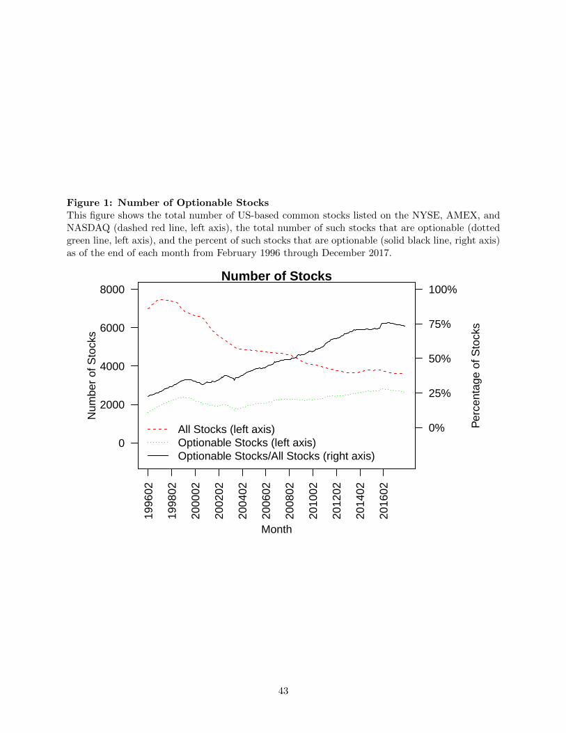
Figure 1: Number of Optionable StocksThis figure shows the total number of US-based common stocks listed on the NYSE, AMEX, andNASDAQ (dashed red line, left axis), the total number of such stocks that are optionable (dottedgreen line, left axis), and the percent of such stocks that are optionable (solid black line, right axis)as of the end of each month from February 1996 through December 2017.

Number of Stocks

0

2000

4000

6000

8000

Num

ber

of S

tock

s

1996

02

1998

02

2000

02

2002

02

2004

02

2006

02

2008

02

2010

02

2012

02

2014

02

2016

02

0%

25%

50%

75%

100%

Month

Per

cent

age

of S

tock

s

All Stocks (left axis)Optionable Stocks (left axis)Optionable Stocks/All Stocks (right axis)

43

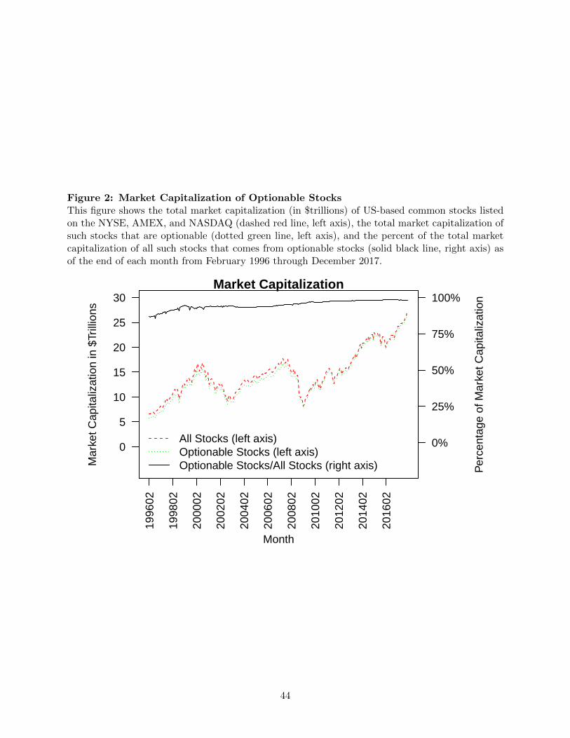
Figure 2: Market Capitalization of Optionable StocksThis figure shows the total market capitalization (in $trillions) of US-based common stocks listedon the NYSE, AMEX, and NASDAQ (dashed red line, left axis), the total market capitalization ofsuch stocks that are optionable (dotted green line, left axis), and the percent of the total marketcapitalization of all such stocks that comes from optionable stocks (solid black line, right axis) asof the end of each month from February 1996 through December 2017.

Market Capitalization

0

5

10

15

20

25

30

Mar

ket C

apita

lizat

ion

in $

Trill

ions

1996

02

1998

02

2000

02

2002

02

2004

02

2006

02

2008

02

2010

02

2012

02

2014

02

2016

02

0%

25%

50%

75%

100%

Month

Per

cent

age

of M

arke

t Cap

italiz

atio

n

All Stocks (left axis)Optionable Stocks (left axis)Optionable Stocks/All Stocks (right axis)

44

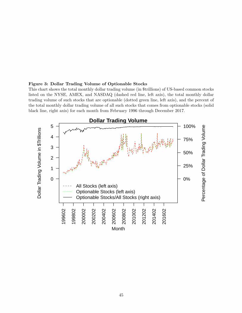
Figure 3: Dollar Trading Volume of Optionable StocksThis chart shows the total monthly dollar trading volume (in $trillions) of US-based common stockslisted on the NYSE, AMEX, and NASDAQ (dashed red line, left axis), the total monthly dollartrading volume of such stocks that are optionable (dotted green line, left axis), and the percent ofthe total monthly dollar trading volume of all such stocks that comes from optionable stocks (solidblack line, right axis) for each month from February 1996 through December 2017.

Dollar Trading Volume

0

1

2

3

4

5

Dol

lar

Trad

ing

Vol

ume

in $

Trill

ions

1996

02

1998

02

2000

02

2002

02

2004

02

2006

02

2008

02

2010

02

2012

02

2014

02

2016

02

0%

25%

50%

75%

100%

Month

Per

cent

age

of D

olla

r Tr

adin

g V

olum

e

All Stocks (left axis)Optionable Stocks (left axis)Optionable Stocks/All Stocks (right axis)

45

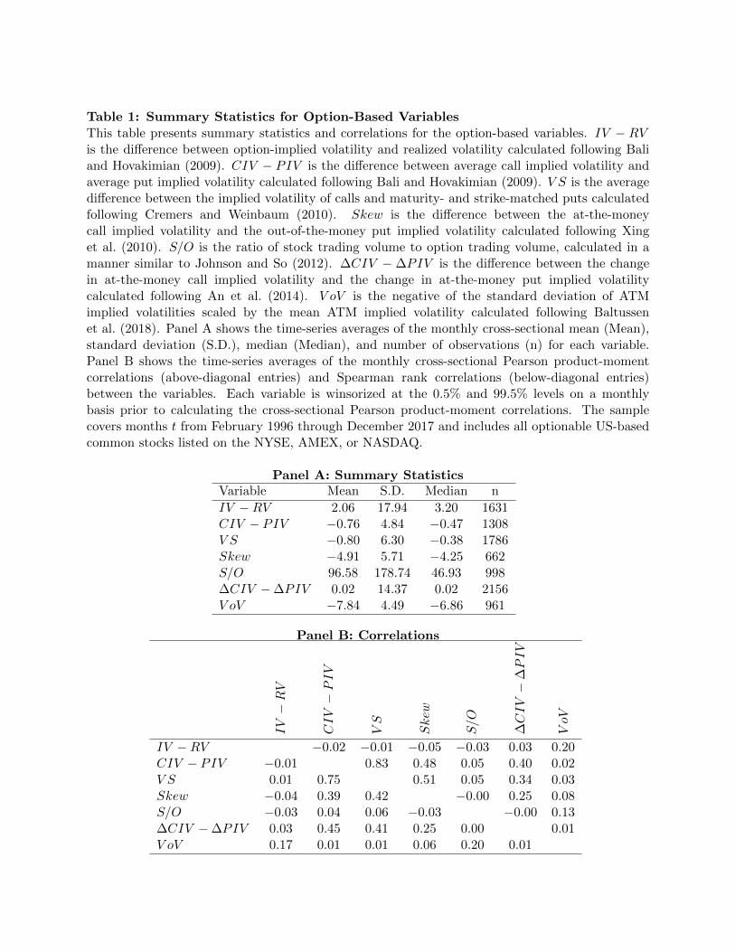
Table 1: Summary Statistics for Option-Based VariablesThis table presents summary statistics and correlations for the option-based variables. IV − RVis the difference between option-implied volatility and realized volatility calculated following Baliand Hovakimian (2009). CIV − PIV is the difference between average call implied volatility andaverage put implied volatility calculated following Bali and Hovakimian (2009). V S is the averagedifference between the implied volatility of calls and maturity- and strike-matched puts calculatedfollowing Cremers and Weinbaum (2010). Skew is the difference between the at-the-moneycall implied volatility and the out-of-the-money put implied volatility calculated following Xinget al. (2010). S/O is the ratio of stock trading volume to option trading volume, calculated in amanner similar to Johnson and So (2012). ∆CIV − ∆PIV is the difference between the changein at-the-money call implied volatility and the change in at-the-money put implied volatilitycalculated following An et al. (2014). V oV is the negative of the standard deviation of ATMimplied volatilities scaled by the mean ATM implied volatility calculated following Baltussenet al. (2018). Panel A shows the time-series averages of the monthly cross-sectional mean (Mean),standard deviation (S.D.), median (Median), and number of observations (n) for each variable.Panel B shows the time-series averages of the monthly cross-sectional Pearson product-momentcorrelations (above-diagonal entries) and Spearman rank correlations (below-diagonal entries)between the variables. Each variable is winsorized at the 0.5% and 99.5% levels on a monthlybasis prior to calculating the cross-sectional Pearson product-moment correlations. The samplecovers months t from February 1996 through December 2017 and includes all optionable US-basedcommon stocks listed on the NYSE, AMEX, or NASDAQ.

Panel A: Summary StatisticsVariable Mean S.D. Median n

IV −RV 2.06 17.94 3.20 1631CIV − PIV −0.76 4.84 −0.47 1308V S −0.80 6.30 −0.38 1786Skew −4.91 5.71 −4.25 662S/O 96.58 178.74 46.93 998∆CIV −∆PIV 0.02 14.37 0.02 2156V oV −7.84 4.49 −6.86 961

Panel B: Correlations

IV−RV

CIV−PIV

VS

Skew

S/O

∆CIV−

∆PIV

VoV

IV −RV −0.02 −0.01 −0.05 −0.03 0.03 0.20CIV − PIV −0.01 0.83 0.48 0.05 0.40 0.02V S 0.01 0.75 0.51 0.05 0.34 0.03Skew −0.04 0.39 0.42 −0.00 0.25 0.08S/O −0.03 0.04 0.06 −0.03 −0.00 0.13∆CIV −∆PIV 0.03 0.45 0.41 0.25 0.00 0.01V oV 0.17 0.01 0.01 0.06 0.20 0.01

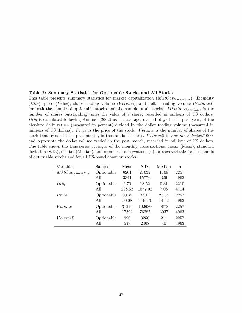
Table 2: Summary Statistics for Optionable Stocks and All StocksThis table presents summary statistics for market capitalization (MktCapShareclass), illiquidity(Illiq), price (Price), share trading volume (V olume), and dollar trading volume (V olume$)for both the sample of optionable stocks and the sample of all stocks. MktCapShareClass is thenumber of shares outstanding times the value of a share, recorded in millions of US dollars.Illiq is calculated following Amihud (2002) as the average, over all days in the past year, of theabsolute daily return (measured in percent) divided by the dollar trading volume (measured inmillions of US dollars). Price is the price of the stock. V olume is the number of shares of thestock that traded in the past month, in thousands of shares. V olume$ is V olume × Price/1000,and represents the dollar volume traded in the past month, recorded in millions of US dollars.The table shows the time-series averages of the monthly cross-sectional mean (Mean), standarddeviation (S.D.), median (Median), and number of observations (n) for each variable for the sampleof optionable stocks and for all US-based common stocks.

Variable Sample Mean S.D. Median n

MktCapShareClass Optionable 6201 21632 1168 2257All 3341 15776 329 4963

Illiq Optionable 2.70 18.52 0.31 2210All 298.52 1577.02 7.08 4714

Price Optionable 30.35 33.17 23.04 2257All 50.08 1740.70 14.52 4963

V olume Optionable 31356 102630 9678 2257All 17399 76285 3037 4963

V olume$ Optionable 990 3250 211 2257All 537 2408 40 4963

47

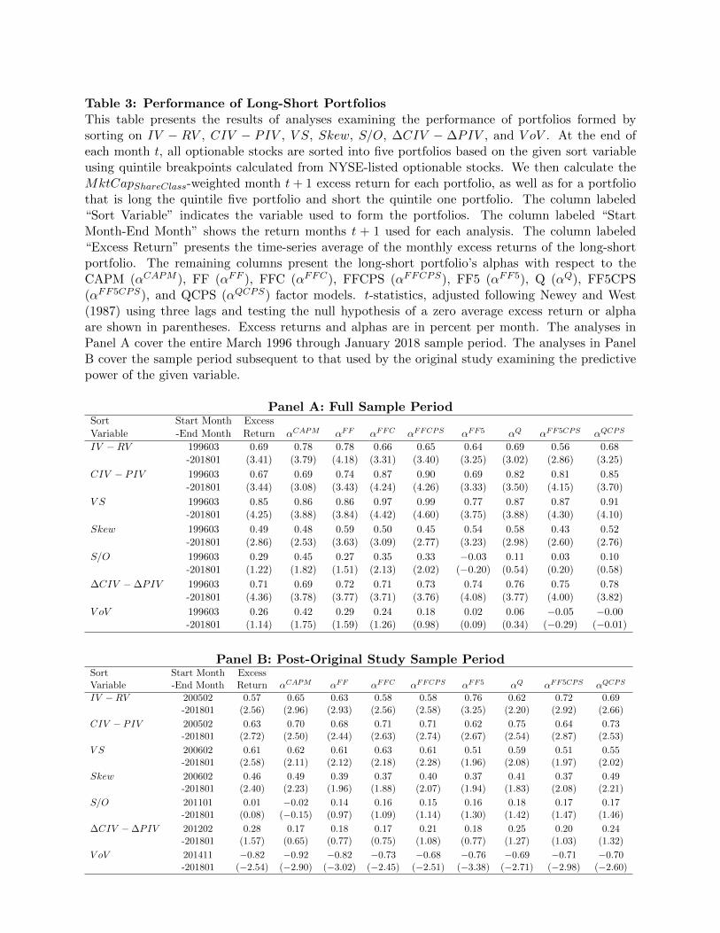
Table 3: Performance of Long-Short PortfoliosThis table presents the results of analyses examining the performance of portfolios formed bysorting on IV − RV , CIV − PIV , V S, Skew, S/O, ∆CIV − ∆PIV , and V oV . At the end ofeach month t, all optionable stocks are sorted into five portfolios based on the given sort variableusing quintile breakpoints calculated from NYSE-listed optionable stocks. We then calculate theMktCapShareClass-weighted month t+ 1 excess return for each portfolio, as well as for a portfoliothat is long the quintile five portfolio and short the quintile one portfolio. The column labeled“Sort Variable” indicates the variable used to form the portfolios. The column labeled “StartMonth-End Month” shows the return months t + 1 used for each analysis. The column labeled“Excess Return” presents the time-series average of the monthly excess returns of the long-shortportfolio. The remaining columns present the long-short portfolio’s alphas with respect to theCAPM (αCAPM ), FF (αFF ), FFC (αFFC), FFCPS (αFFCPS), FF5 (αFF5), Q (αQ), FF5CPS(αFF5CPS), and QCPS (αQCPS) factor models. t-statistics, adjusted following Newey and West(1987) using three lags and testing the null hypothesis of a zero average excess return or alphaare shown in parentheses. Excess returns and alphas are in percent per month. The analyses inPanel A cover the entire March 1996 through January 2018 sample period. The analyses in PanelB cover the sample period subsequent to that used by the original study examining the predictivepower of the given variable.

Panel A: Full Sample PeriodSort Start Month ExcessVariable -End Month Return αCAPM αFF αFFC αFFCPS αFF5 αQ αFF5CPS αQCPS

IV −RV 199603 0.69 0.78 0.78 0.66 0.65 0.64 0.69 0.56 0.68-201801 (3.41) (3.79) (4.18) (3.31) (3.40) (3.25) (3.02) (2.86) (3.25)

CIV − PIV 199603 0.67 0.69 0.74 0.87 0.90 0.69 0.82 0.81 0.85-201801 (3.44) (3.08) (3.43) (4.24) (4.26) (3.33) (3.50) (4.15) (3.70)

V S 199603 0.85 0.86 0.86 0.97 0.99 0.77 0.87 0.87 0.91-201801 (4.25) (3.88) (3.84) (4.42) (4.60) (3.75) (3.88) (4.30) (4.10)

Skew 199603 0.49 0.48 0.59 0.50 0.45 0.54 0.58 0.43 0.52-201801 (2.86) (2.53) (3.63) (3.09) (2.77) (3.23) (2.98) (2.60) (2.76)

S/O 199603 0.29 0.45 0.27 0.35 0.33 −0.03 0.11 0.03 0.10-201801 (1.22) (1.82) (1.51) (2.13) (2.02) (−0.20) (0.54) (0.20) (0.58)

∆CIV −∆PIV 199603 0.71 0.69 0.72 0.71 0.73 0.74 0.76 0.75 0.78-201801 (4.36) (3.78) (3.77) (3.71) (3.76) (4.08) (3.77) (4.00) (3.82)

V oV 199603 0.26 0.42 0.29 0.24 0.18 0.02 0.06 −0.05 −0.00-201801 (1.14) (1.75) (1.59) (1.26) (0.98) (0.09) (0.34) (−0.29) (−0.01)

Panel B: Post-Original Study Sample PeriodSort Start Month ExcessVariable -End Month Return αCAPM αFF αFFC αFFCPS αFF5 αQ αFF5CPS αQCPS

IV −RV 200502 0.57 0.65 0.63 0.58 0.58 0.76 0.62 0.72 0.69-201801 (2.56) (2.96) (2.93) (2.56) (2.58) (3.25) (2.20) (2.92) (2.66)

CIV − PIV 200502 0.63 0.70 0.68 0.71 0.71 0.62 0.75 0.64 0.73-201801 (2.72) (2.50) (2.44) (2.63) (2.74) (2.67) (2.54) (2.87) (2.53)

V S 200602 0.61 0.62 0.61 0.63 0.61 0.51 0.59 0.51 0.55-201801 (2.58) (2.11) (2.12) (2.18) (2.28) (1.96) (2.08) (1.97) (2.02)

Skew 200602 0.46 0.49 0.39 0.37 0.40 0.37 0.41 0.37 0.49-201801 (2.40) (2.23) (1.96) (1.88) (2.07) (1.94) (1.83) (2.08) (2.21)

S/O 201101 0.01 −0.02 0.14 0.16 0.15 0.16 0.18 0.17 0.17-201801 (0.08) (−0.15) (0.97) (1.09) (1.14) (1.30) (1.42) (1.47) (1.46)

∆CIV −∆PIV 201202 0.28 0.17 0.18 0.17 0.21 0.18 0.25 0.20 0.24-201801 (1.57) (0.65) (0.77) (0.75) (1.08) (0.77) (1.27) (1.03) (1.32)

V oV 201411 −0.82 −0.92 −0.82 −0.73 −0.68 −0.76 −0.69 −0.71 −0.70-201801 (−2.54) (−2.90) (−3.02) (−2.45) (−2.51) (−3.38) (−2.71) (−2.98) (−2.60)

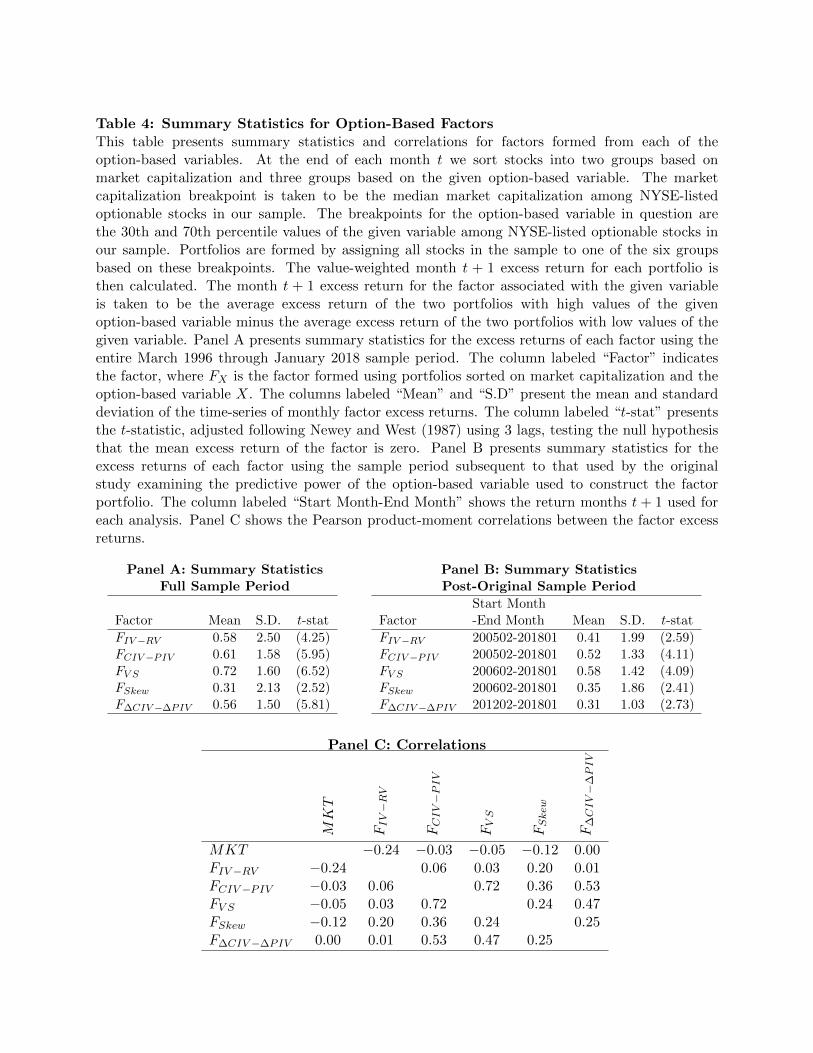
Table 4: Summary Statistics for Option-Based FactorsThis table presents summary statistics and correlations for factors formed from each of theoption-based variables. At the end of each month t we sort stocks into two groups based onmarket capitalization and three groups based on the given option-based variable. The marketcapitalization breakpoint is taken to be the median market capitalization among NYSE-listedoptionable stocks in our sample. The breakpoints for the option-based variable in question arethe 30th and 70th percentile values of the given variable among NYSE-listed optionable stocks inour sample. Portfolios are formed by assigning all stocks in the sample to one of the six groupsbased on these breakpoints. The value-weighted month t + 1 excess return for each portfolio isthen calculated. The month t + 1 excess return for the factor associated with the given variableis taken to be the average excess return of the two portfolios with high values of the givenoption-based variable minus the average excess return of the two portfolios with low values of thegiven variable. Panel A presents summary statistics for the excess returns of each factor using theentire March 1996 through January 2018 sample period. The column labeled “Factor” indicatesthe factor, where FX is the factor formed using portfolios sorted on market capitalization and theoption-based variable X. The columns labeled “Mean” and “S.D” present the mean and standarddeviation of the time-series of monthly factor excess returns. The column labeled “t-stat” presentsthe t-statistic, adjusted following Newey and West (1987) using 3 lags, testing the null hypothesisthat the mean excess return of the factor is zero. Panel B presents summary statistics for theexcess returns of each factor using the sample period subsequent to that used by the originalstudy examining the predictive power of the option-based variable used to construct the factorportfolio. The column labeled “Start Month-End Month” shows the return months t + 1 used foreach analysis. Panel C shows the Pearson product-moment correlations between the factor excessreturns.

Panel A: Summary Statistics Panel B: Summary StatisticsFull Sample Period Post-Original Sample Period

Factor Mean S.D. t-stat

FIV−RV 0.58 2.50 (4.25)FCIV−PIV 0.61 1.58 (5.95)FV S 0.72 1.60 (6.52)FSkew 0.31 2.13 (2.52)F∆CIV−∆PIV 0.56 1.50 (5.81)

Start MonthFactor -End Month Mean S.D. t-stat

FIV−RV 200502-201801 0.41 1.99 (2.59)FCIV−PIV 200502-201801 0.52 1.33 (4.11)FV S 200602-201801 0.58 1.42 (4.09)FSkew 200602-201801 0.35 1.86 (2.41)F∆CIV−∆PIV 201202-201801 0.31 1.03 (2.73)

Panel C: Correlations

MKT

FIV−RV

FCIV−PIV

FVS

FSkew

F∆CIV−

∆PIV

MKT −0.24 −0.03 −0.05 −0.12 0.00FIV−RV −0.24 0.06 0.03 0.20 0.01FCIV−PIV −0.03 0.06 0.72 0.36 0.53FV S −0.05 0.03 0.72 0.24 0.47FSkew −0.12 0.20 0.36 0.24 0.25F∆CIV−∆PIV 0.00 0.01 0.53 0.47 0.25

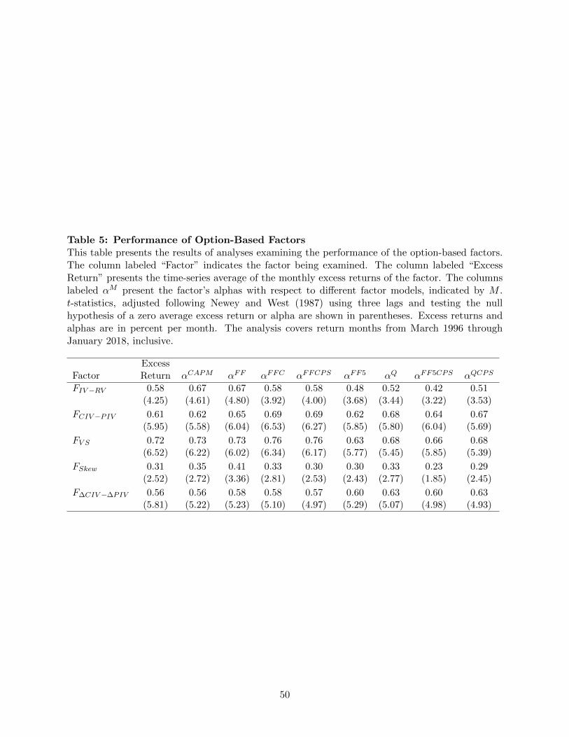
Table 5: Performance of Option-Based FactorsThis table presents the results of analyses examining the performance of the option-based factors.The column labeled “Factor” indicates the factor being examined. The column labeled “ExcessReturn” presents the time-series average of the monthly excess returns of the factor. The columnslabeled αM present the factor’s alphas with respect to different factor models, indicated by M .t-statistics, adjusted following Newey and West (1987) using three lags and testing the nullhypothesis of a zero average excess return or alpha are shown in parentheses. Excess returns andalphas are in percent per month. The analysis covers return months from March 1996 throughJanuary 2018, inclusive.

ExcessFactor Return αCAPM αFF αFFC αFFCPS αFF5 αQ αFF5CPS αQCPS

FIV−RV 0.58 0.67 0.67 0.58 0.58 0.48 0.52 0.42 0.51(4.25) (4.61) (4.80) (3.92) (4.00) (3.68) (3.44) (3.22) (3.53)

FCIV−PIV 0.61 0.62 0.65 0.69 0.69 0.62 0.68 0.64 0.67(5.95) (5.58) (6.04) (6.53) (6.27) (5.85) (5.80) (6.04) (5.69)

FV S 0.72 0.73 0.73 0.76 0.76 0.63 0.68 0.66 0.68(6.52) (6.22) (6.02) (6.34) (6.17) (5.77) (5.45) (5.85) (5.39)

FSkew 0.31 0.35 0.41 0.33 0.30 0.30 0.33 0.23 0.29(2.52) (2.72) (3.36) (2.81) (2.53) (2.43) (2.77) (1.85) (2.45)

F∆CIV−∆PIV 0.56 0.56 0.58 0.58 0.57 0.60 0.63 0.60 0.63(5.81) (5.22) (5.23) (5.10) (4.97) (5.29) (5.07) (4.98) (4.93)

50

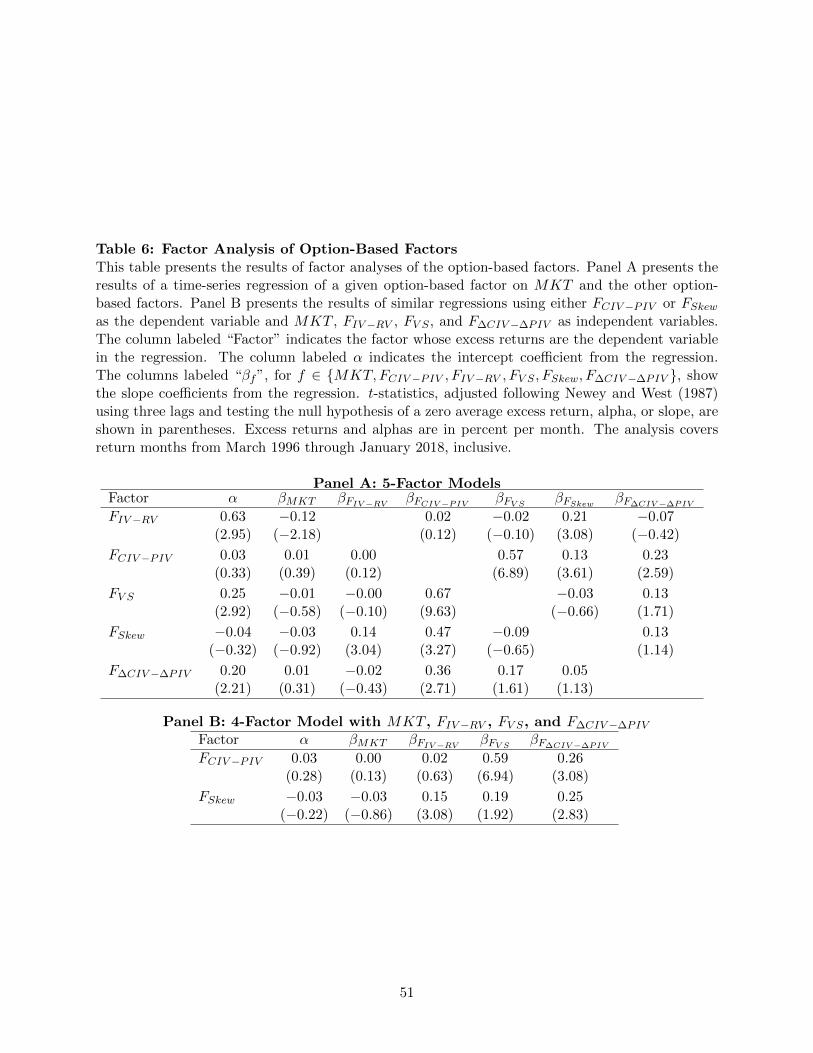
Table 6: Factor Analysis of Option-Based FactorsThis table presents the results of factor analyses of the option-based factors. Panel A presents theresults of a time-series regression of a given option-based factor on MKT and the other option-based factors. Panel B presents the results of similar regressions using either FCIV−PIV or FSkew

as the dependent variable and MKT , FIV−RV , FV S , and F∆CIV−∆PIV as independent variables.The column labeled “Factor” indicates the factor whose excess returns are the dependent variablein the regression. The column labeled α indicates the intercept coefficient from the regression.The columns labeled “βf”, for f ∈ {MKT,FCIV−PIV , FIV−RV , FV S , FSkew, F∆CIV−∆PIV }, showthe slope coefficients from the regression. t-statistics, adjusted following Newey and West (1987)using three lags and testing the null hypothesis of a zero average excess return, alpha, or slope, areshown in parentheses. Excess returns and alphas are in percent per month. The analysis coversreturn months from March 1996 through January 2018, inclusive.

Panel A: 5-Factor ModelsFactor α βMKT βFIV−RV

βFCIV−PIVβFV S

βFSkewβF∆CIV−∆PIV

FIV−RV 0.63 −0.12 0.02 −0.02 0.21 −0.07(2.95) (−2.18) (0.12) (−0.10) (3.08) (−0.42)

FCIV−PIV 0.03 0.01 0.00 0.57 0.13 0.23(0.33) (0.39) (0.12) (6.89) (3.61) (2.59)

FV S 0.25 −0.01 −0.00 0.67 −0.03 0.13(2.92) (−0.58) (−0.10) (9.63) (−0.66) (1.71)

FSkew −0.04 −0.03 0.14 0.47 −0.09 0.13(−0.32) (−0.92) (3.04) (3.27) (−0.65) (1.14)

F∆CIV−∆PIV 0.20 0.01 −0.02 0.36 0.17 0.05(2.21) (0.31) (−0.43) (2.71) (1.61) (1.13)

Panel B: 4-Factor Model with MKT , FIV−RV , FV S, and F∆CIV−∆PIV

Factor α βMKT βFIV−RVβFV S

βF∆CIV−∆PIV

FCIV−PIV 0.03 0.00 0.02 0.59 0.26(0.28) (0.13) (0.63) (6.94) (3.08)

FSkew −0.03 −0.03 0.15 0.19 0.25(−0.22) (−0.86) (3.08) (1.92) (2.83)

51

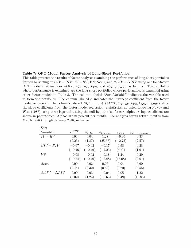
Table 7: OPT Model Factor Analysis of Long-Short PortfoliosThis table presents the results of factor analyses examining the performance of long-short portfoliosformed by sorting on CIV −PIV , IV −RV , V S, Skew, and ∆CIV −∆PIV using our four-factorOPT model that includes MKT , FIV−RV , FV S , and F∆CIV−∆PIV as factors. The portfolioswhose performance is examined are the long-short portfolios whose performance is examined usingother factor models in Table 3. The column labeled “Sort Variable” indicates the variable usedto form the portfolios. The column labeled α indicates the intercept coefficient from the factormodel regression. The columns labeled “βf”, for f ∈ {MKT,FIV−RV , FV S , F∆CIV−∆PIV } showthe slope coefficients from the factor model regression. t-statistics, adjusted following Newey andWest (1987) using three lags and testing the null hypothesis of a zero alpha or slope coefficient areshown in parentheses. Alphas are in percent per month. The analysis covers return months fromMarch 1996 through January 2018, inclusive.

SortVariable αOPT βMKT βFIV−RV

βFV SβF∆CIV−∆PIV

IV −RV 0.03 0.04 1.28 −0.40 0.33(0.23) (1.87) (25.57) (−2.73) (2.57)

CIV − PIV −0.07 −0.02 −0.17 0.98 0.28(−0.46) (−0.49) (−2.23) (5.77) (1.61)

V S −0.08 −0.02 −0.18 1.24 0.29(−0.54) (−0.40) (−2.88) (13.08) (2.61)

Skew 0.09 0.02 0.05 0.04 0.60(0.44) (0.32) (0.59) (0.20) (4.56)

∆CIV −∆PIV 0.00 0.03 −0.04 0.05 1.22(0.02) (1.25) (−0.63) (0.48) (10.83)

52

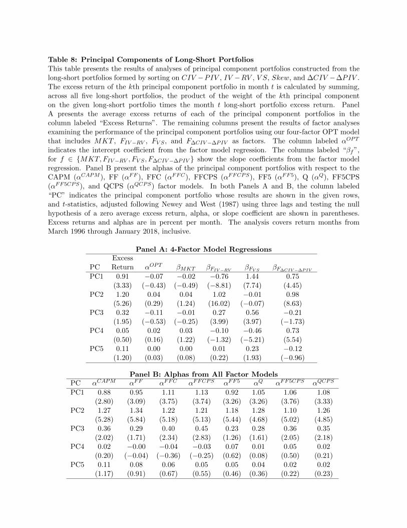
Table 8: Principal Components of Long-Short PortfoliosThis table presents the results of analyses of principal component portfolios constructed from thelong-short portfolios formed by sorting on CIV −PIV , IV −RV , V S, Skew, and ∆CIV −∆PIV .The excess return of the kth principal component portfolio in month t is calculated by summing,across all five long-short portfolios, the product of the weight of the kth principal componenton the given long-short portfolio times the month t long-short portfolio excess return. PanelA presents the average excess returns of each of the principal component portfolios in thecolumn labeled “Excess Returns”. The remaining columns present the results of factor analysesexamining the performance of the principal component portfolios using our four-factor OPT modelthat includes MKT , FIV−RV , FV S , and F∆CIV−∆PIV as factors. The column labeled αOPT

indicates the intercept coefficient from the factor model regression. The columns labeled “βf”,for f ∈ {MKT,FIV−RV , FV S , F∆CIV−∆PIV } show the slope coefficients from the factor modelregression. Panel B present the alphas of the principal component portfolios with respect to theCAPM (αCAPM ), FF (αFF ), FFC (αFFC), FFCPS (αFFCPS), FF5 (αFF5), Q (αQ), FF5CPS(αFF5CPS), and QCPS (αQCPS) factor models. In both Panels A and B, the column labeled“PC” indicates the principal component portfolio whose results are shown in the given rows,and t-statistics, adjusted following Newey and West (1987) using three lags and testing the nullhypothesis of a zero average excess return, alpha, or slope coefficient are shown in parentheses.Excess returns and alphas are in percent per month. The analysis covers return months fromMarch 1996 through January 2018, inclusive.

Panel A: 4-Factor Model RegressionsExcess

PC Return αOPT βMKT βFIV−RVβFV S

βF∆CIV−∆PIV

PC1 0.91 −0.07 −0.02 −0.76 1.44 0.75(3.33) (−0.43) (−0.49) (−8.81) (7.74) (4.45)

PC2 1.20 0.04 0.04 1.02 −0.01 0.98(5.26) (0.29) (1.24) (16.02) (−0.07) (8.63)

PC3 0.32 −0.11 −0.01 0.27 0.56 −0.21(1.95) (−0.53) (−0.25) (3.99) (3.97) (−1.73)

PC4 0.05 0.02 0.03 −0.10 −0.46 0.73(0.50) (0.16) (1.22) (−1.32) (−5.21) (5.54)

PC5 0.11 0.00 0.00 0.01 0.23 −0.12(1.20) (0.03) (0.08) (0.22) (1.93) (−0.96)

Panel B: Alphas from All Factor ModelsPC αCAPM αFF αFFC αFFCPS αFF5 αQ αFF5CPS αQCPS

PC1 0.88 0.95 1.11 1.13 0.92 1.05 1.06 1.08(2.80) (3.09) (3.75) (3.74) (3.26) (3.26) (3.76) (3.33)

PC2 1.27 1.34 1.22 1.21 1.18 1.28 1.10 1.26(5.28) (5.84) (5.18) (5.13) (5.44) (4.68) (5.02) (4.85)

PC3 0.36 0.29 0.40 0.45 0.23 0.28 0.36 0.35(2.02) (1.71) (2.34) (2.83) (1.26) (1.61) (2.05) (2.18)

PC4 0.02 −0.00 −0.04 −0.03 0.07 0.01 0.05 0.02(0.20) (−0.04) (−0.36) (−0.25) (0.62) (0.08) (0.50) (0.21)

PC5 0.11 0.08 0.06 0.05 0.05 0.04 0.02 0.02(1.17) (0.91) (0.67) (0.55) (0.46) (0.36) (0.22) (0.23)

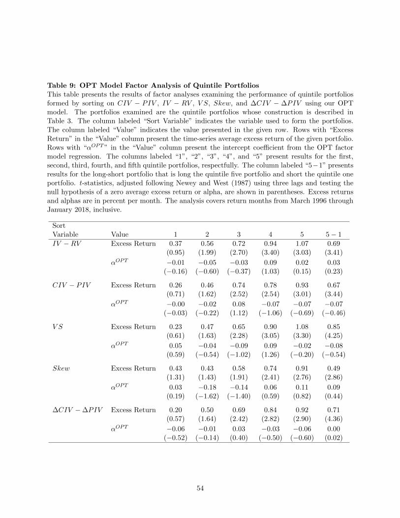
Table 9: OPT Model Factor Analysis of Quintile PortfoliosThis table presents the results of factor analyses examining the performance of quintile portfoliosformed by sorting on CIV − PIV , IV − RV , V S, Skew, and ∆CIV − ∆PIV using our OPTmodel. The portfolios examined are the quintile portfolios whose construction is described inTable 3. The column labeled “Sort Variable” indicates the variable used to form the portfolios.The column labeled “Value” indicates the value presented in the given row. Rows with “ExcessReturn” in the “Value” column present the time-series average excess return of the given portfolio.Rows with “αOPT ” in the “Value” column present the intercept coefficient from the OPT factormodel regression. The columns labeled “1”, “2”, “3”, “4”, and “5” present results for the first,second, third, fourth, and fifth quintile portfolios, respectfully. The column labeled “5−1” presentsresults for the long-short portfolio that is long the quintile five portfolio and short the quintile oneportfolio. t-statistics, adjusted following Newey and West (1987) using three lags and testing thenull hypothesis of a zero average excess return or alpha, are shown in parentheses. Excess returnsand alphas are in percent per month. The analysis covers return months from March 1996 throughJanuary 2018, inclusive.

SortVariable Value 1 2 3 4 5 5− 1

IV −RV Excess Return 0.37 0.56 0.72 0.94 1.07 0.69(0.95) (1.99) (2.70) (3.40) (3.03) (3.41)

αOPT −0.01 −0.05 −0.03 0.09 0.02 0.03(−0.16) (−0.60) (−0.37) (1.03) (0.15) (0.23)

CIV − PIV Excess Return 0.26 0.46 0.74 0.78 0.93 0.67(0.71) (1.62) (2.52) (2.54) (3.01) (3.44)

αOPT −0.00 −0.02 0.08 −0.07 −0.07 −0.07(−0.03) (−0.22) (1.12) (−1.06) (−0.69) (−0.46)

V S Excess Return 0.23 0.47 0.65 0.90 1.08 0.85(0.61) (1.63) (2.28) (3.05) (3.30) (4.25)

αOPT 0.05 −0.04 −0.09 0.09 −0.02 −0.08(0.59) (−0.54) (−1.02) (1.26) (−0.20) (−0.54)

Skew Excess Return 0.43 0.43 0.58 0.74 0.91 0.49(1.31) (1.43) (1.91) (2.41) (2.76) (2.86)

αOPT 0.03 −0.18 −0.14 0.06 0.11 0.09(0.19) (−1.62) (−1.40) (0.59) (0.82) (0.44)

∆CIV −∆PIV Excess Return 0.20 0.50 0.69 0.84 0.92 0.71(0.57) (1.64) (2.42) (2.82) (2.90) (4.36)

αOPT −0.06 −0.01 0.03 −0.03 −0.06 0.00(−0.52) (−0.14) (0.40) (−0.50) (−0.60) (0.02)

54

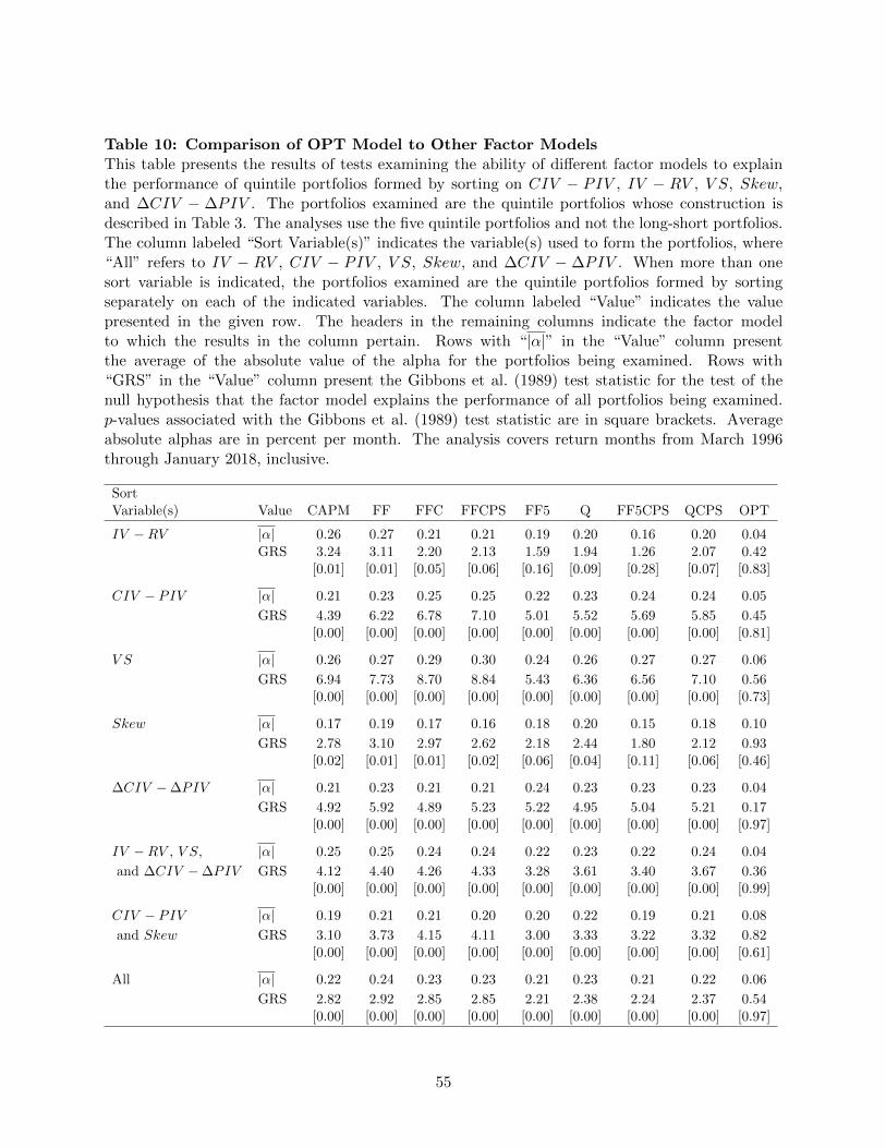
Table 10: Comparison of OPT Model to Other Factor ModelsThis table presents the results of tests examining the ability of different factor models to explainthe performance of quintile portfolios formed by sorting on CIV − PIV , IV − RV , V S, Skew,and ∆CIV − ∆PIV . The portfolios examined are the quintile portfolios whose construction isdescribed in Table 3. The analyses use the five quintile portfolios and not the long-short portfolios.The column labeled “Sort Variable(s)” indicates the variable(s) used to form the portfolios, where“All” refers to IV − RV , CIV − PIV , V S, Skew, and ∆CIV − ∆PIV . When more than onesort variable is indicated, the portfolios examined are the quintile portfolios formed by sortingseparately on each of the indicated variables. The column labeled “Value” indicates the valuepresented in the given row. The headers in the remaining columns indicate the factor modelto which the results in the column pertain. Rows with “|α|” in the “Value” column presentthe average of the absolute value of the alpha for the portfolios being examined. Rows with“GRS” in the “Value” column present the Gibbons et al. (1989) test statistic for the test of thenull hypothesis that the factor model explains the performance of all portfolios being examined.p-values associated with the Gibbons et al. (1989) test statistic are in square brackets. Averageabsolute alphas are in percent per month. The analysis covers return months from March 1996through January 2018, inclusive.

SortVariable(s) Value CAPM FF FFC FFCPS FF5 Q FF5CPS QCPS OPT

IV −RV |α| 0.26 0.27 0.21 0.21 0.19 0.20 0.16 0.20 0.04GRS 3.24 3.11 2.20 2.13 1.59 1.94 1.26 2.07 0.42

[0.01] [0.01] [0.05] [0.06] [0.16] [0.09] [0.28] [0.07] [0.83]

CIV − PIV |α| 0.21 0.23 0.25 0.25 0.22 0.23 0.24 0.24 0.05

GRS 4.39 6.22 6.78 7.10 5.01 5.52 5.69 5.85 0.45[0.00] [0.00] [0.00] [0.00] [0.00] [0.00] [0.00] [0.00] [0.81]

V S |α| 0.26 0.27 0.29 0.30 0.24 0.26 0.27 0.27 0.06

GRS 6.94 7.73 8.70 8.84 5.43 6.36 6.56 7.10 0.56[0.00] [0.00] [0.00] [0.00] [0.00] [0.00] [0.00] [0.00] [0.73]

Skew |α| 0.17 0.19 0.17 0.16 0.18 0.20 0.15 0.18 0.10

GRS 2.78 3.10 2.97 2.62 2.18 2.44 1.80 2.12 0.93[0.02] [0.01] [0.01] [0.02] [0.06] [0.04] [0.11] [0.06] [0.46]

∆CIV −∆PIV |α| 0.21 0.23 0.21 0.21 0.24 0.23 0.23 0.23 0.04

GRS 4.92 5.92 4.89 5.23 5.22 4.95 5.04 5.21 0.17[0.00] [0.00] [0.00] [0.00] [0.00] [0.00] [0.00] [0.00] [0.97]

IV −RV , V S, |α| 0.25 0.25 0.24 0.24 0.22 0.23 0.22 0.24 0.04

and ∆CIV −∆PIV GRS 4.12 4.40 4.26 4.33 3.28 3.61 3.40 3.67 0.36[0.00] [0.00] [0.00] [0.00] [0.00] [0.00] [0.00] [0.00] [0.99]

CIV − PIV |α| 0.19 0.21 0.21 0.20 0.20 0.22 0.19 0.21 0.08

and Skew GRS 3.10 3.73 4.15 4.11 3.00 3.33 3.22 3.32 0.82[0.00] [0.00] [0.00] [0.00] [0.00] [0.00] [0.00] [0.00] [0.61]

All |α| 0.22 0.24 0.23 0.23 0.21 0.23 0.21 0.22 0.06

GRS 2.82 2.92 2.85 2.85 2.21 2.38 2.24 2.37 0.54[0.00] [0.00] [0.00] [0.00] [0.00] [0.00] [0.00] [0.00] [0.97]

55

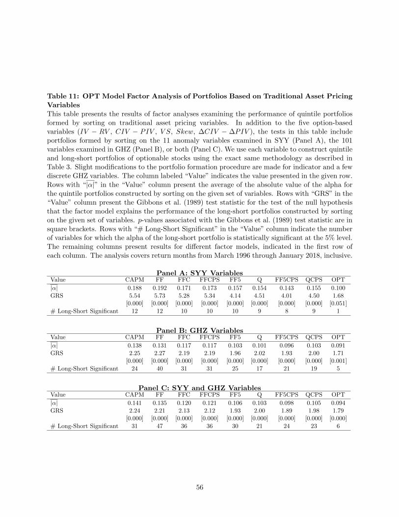
Table 11: OPT Model Factor Analysis of Portfolios Based on Traditional Asset PricingVariablesThis table presents the results of factor analyses examining the performance of quintile portfoliosformed by sorting on traditional asset pricing variables. In addition to the five option-basedvariables (IV − RV , CIV − PIV , V S, Skew, ∆CIV − ∆PIV ), the tests in this table includeportfolios formed by sorting on the 11 anomaly variables examined in SYY (Panel A), the 101variables examined in GHZ (Panel B), or both (Panel C). We use each variable to construct quintileand long-short portfolios of optionable stocks using the exact same methodology as described inTable 3. Slight modifications to the portfolio formation procedure are made for indicator and a fewdiscrete GHZ variables. The column labeled “Value” indicates the value presented in the given row.Rows with “|α|” in the “Value” column present the average of the absolute value of the alpha forthe quintile portfolios constructed by sorting on the given set of variables. Rows with “GRS” in the“Value” column present the Gibbons et al. (1989) test statistic for the test of the null hypothesisthat the factor model explains the performance of the long-short portfolios constructed by sortingon the given set of variables. p-values associated with the Gibbons et al. (1989) test statistic are insquare brackets. Rows with “# Long-Short Significant” in the “Value” column indicate the numberof variables for which the alpha of the long-short portfolio is statistically significant at the 5% level.The remaining columns present results for different factor models, indicated in the first row ofeach column. The analysis covers return months from March 1996 through January 2018, inclusive.

Panel A: SYY VariablesValue CAPM FF FFC FFCPS FF5 Q FF5CPS QCPS OPT

|α| 0.188 0.192 0.171 0.173 0.157 0.154 0.143 0.155 0.100GRS 5.54 5.73 5.28 5.34 4.14 4.51 4.01 4.50 1.68

[0.000] [0.000] [0.000] [0.000] [0.000] [0.000] [0.000] [0.000] [0.051]# Long-Short Significant 12 12 10 10 10 9 8 9 1

Panel B: GHZ VariablesValue CAPM FF FFC FFCPS FF5 Q FF5CPS QCPS OPT

|α| 0.138 0.131 0.117 0.117 0.103 0.101 0.096 0.103 0.091GRS 2.25 2.27 2.19 2.19 1.96 2.02 1.93 2.00 1.71

[0.000] [0.000] [0.000] [0.000] [0.000] [0.000] [0.000] [0.000] [0.001]# Long-Short Significant 24 40 31 31 25 17 21 19 5

Panel C: SYY and GHZ VariablesValue CAPM FF FFC FFCPS FF5 Q FF5CPS QCPS OPT

|α| 0.141 0.135 0.120 0.121 0.106 0.103 0.098 0.105 0.094GRS 2.24 2.21 2.13 2.12 1.93 2.00 1.89 1.98 1.79

[0.000] [0.000] [0.000] [0.000] [0.000] [0.000] [0.000] [0.000] [0.000]# Long-Short Significant 31 47 36 36 30 21 24 23 6

56

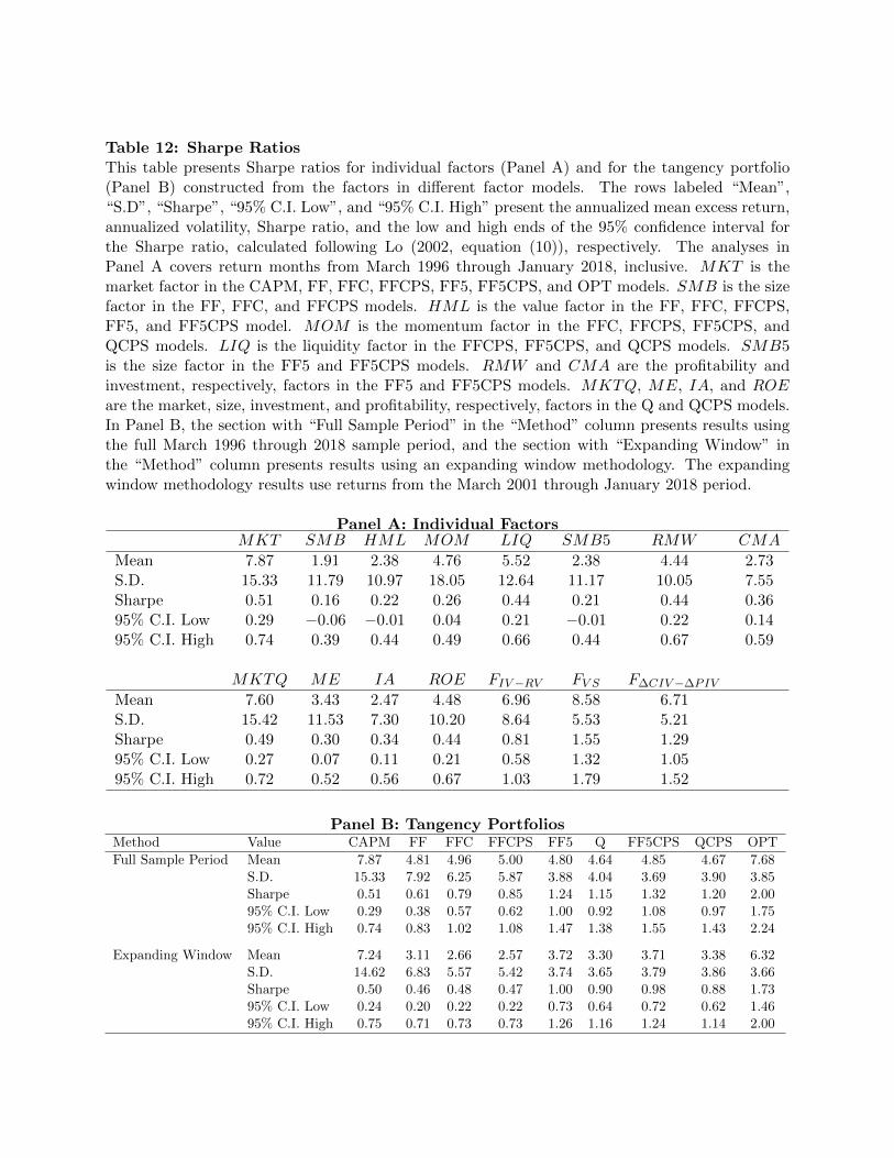
Table 12: Sharpe RatiosThis table presents Sharpe ratios for individual factors (Panel A) and for the tangency portfolio(Panel B) constructed from the factors in different factor models. The rows labeled “Mean”,“S.D”, “Sharpe”, “95% C.I. Low”, and “95% C.I. High” present the annualized mean excess return,annualized volatility, Sharpe ratio, and the low and high ends of the 95% confidence interval forthe Sharpe ratio, calculated following Lo (2002, equation (10)), respectively. The analyses inPanel A covers return months from March 1996 through January 2018, inclusive. MKT is themarket factor in the CAPM, FF, FFC, FFCPS, FF5, FF5CPS, and OPT models. SMB is the sizefactor in the FF, FFC, and FFCPS models. HML is the value factor in the FF, FFC, FFCPS,FF5, and FF5CPS model. MOM is the momentum factor in the FFC, FFCPS, FF5CPS, andQCPS models. LIQ is the liquidity factor in the FFCPS, FF5CPS, and QCPS models. SMB5is the size factor in the FF5 and FF5CPS models. RMW and CMA are the profitability andinvestment, respectively, factors in the FF5 and FF5CPS models. MKTQ, ME, IA, and ROEare the market, size, investment, and profitability, respectively, factors in the Q and QCPS models.In Panel B, the section with “Full Sample Period” in the “Method” column presents results usingthe full March 1996 through 2018 sample period, and the section with “Expanding Window” inthe “Method” column presents results using an expanding window methodology. The expandingwindow methodology results use returns from the March 2001 through January 2018 period.

Panel A: Individual FactorsMKT SMB HML MOM LIQ SMB5 RMW CMA

Mean 7.87 1.91 2.38 4.76 5.52 2.38 4.44 2.73S.D. 15.33 11.79 10.97 18.05 12.64 11.17 10.05 7.55Sharpe 0.51 0.16 0.22 0.26 0.44 0.21 0.44 0.3695% C.I. Low 0.29 −0.06 −0.01 0.04 0.21 −0.01 0.22 0.1495% C.I. High 0.74 0.39 0.44 0.49 0.66 0.44 0.67 0.59

MKTQ ME IA ROE FIV−RV FV S F∆CIV−∆PIV

Mean 7.60 3.43 2.47 4.48 6.96 8.58 6.71S.D. 15.42 11.53 7.30 10.20 8.64 5.53 5.21Sharpe 0.49 0.30 0.34 0.44 0.81 1.55 1.2995% C.I. Low 0.27 0.07 0.11 0.21 0.58 1.32 1.0595% C.I. High 0.72 0.52 0.56 0.67 1.03 1.79 1.52

Panel B: Tangency PortfoliosMethod Value CAPM FF FFC FFCPS FF5 Q FF5CPS QCPS OPT

Full Sample Period Mean 7.87 4.81 4.96 5.00 4.80 4.64 4.85 4.67 7.68S.D. 15.33 7.92 6.25 5.87 3.88 4.04 3.69 3.90 3.85Sharpe 0.51 0.61 0.79 0.85 1.24 1.15 1.32 1.20 2.0095% C.I. Low 0.29 0.38 0.57 0.62 1.00 0.92 1.08 0.97 1.7595% C.I. High 0.74 0.83 1.02 1.08 1.47 1.38 1.55 1.43 2.24

Expanding Window Mean 7.24 3.11 2.66 2.57 3.72 3.30 3.71 3.38 6.32S.D. 14.62 6.83 5.57 5.42 3.74 3.65 3.79 3.86 3.66Sharpe 0.50 0.46 0.48 0.47 1.00 0.90 0.98 0.88 1.7395% C.I. Low 0.24 0.20 0.22 0.22 0.73 0.64 0.72 0.62 1.4695% C.I. High 0.75 0.71 0.73 0.73 1.26 1.16 1.24 1.14 2.00

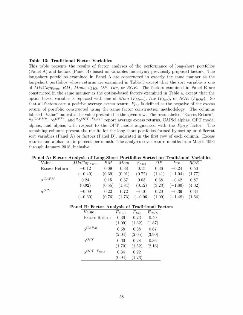
Table 13: Traditional Factor VariablesThis table presents the results of factor analyses of the performance of long-short portfolios(Panel A) and factors (Panel B) based on variables underlying previously-proposed factors. Thelong-short portfolios examined in Panel A are constructed in exactly the same manner as thelong-short portfolios whose returns are examined in Table 3 except that the sort variable is oneof MktCapFirm, BM , Mom, βLIQ, OP , Inv, or ROE. The factors examined in Panel B areconstructed in the same manner as the option-based factors examined in Table 4, except that theoption-based variable is replaced with one of Mom (FMom), Inv (FInv), or ROE (FROE). Sothat all factors earn a positive average excess return, FInv is defined as the negative of the excessreturn of portfolio constructed using the same factor construction methodology. The columnslabeled “Value” indicates the value presented in the given row. The rows labeled “Excess Return”,“αCAPM”, “αOPT ”, and ”αOPT+FROE” report average excess returns, CAPM alphas, OPT modelalphas, and alphas with respect to the OPT model augmented with the FROE factor. Theremaining columns present the results for the long-short portfolios formed by sorting on differentsort variables (Panel A) or factors (Panel B), indicated in the first row of each column. Excessreturns and alphas are in percent per month. The analyses cover return months from March 1996through January 2018, inclusive.

Panel A: Factor Analysis of Long-Short Portfolios Sorted on Traditional VariablesValue MktCapFirm BM Mom βLIQ OP Inv ROE

Excess Return −0.12 0.09 0.38 0.15 0.36 −0.24 0.50(−0.40) (0.39) (0.91) (0.72) (1.41) (−1.04) (1.77)

αCAPM 0.24 0.15 0.67 0.03 0.68 −0.42 0.87(0.92) (0.55) (1.84) (0.12) (3.23) (−1.80) (4.02)

αOPT −0.09 0.22 0.72 −0.01 0.20 −0.36 0.34(−0.30) (0.76) (1.73) (−0.06) (1.09) (−1.48) (1.64)

Panel B: Factor Analysis of Traditional FactorsValue FMom FInv FROE

Excess Return 0.36 0.23 0.40(1.09) (1.32) (1.87)

αCAPM 0.58 0.38 0.67(2.04) (2.05) (3.90)

αOPT 0.60 0.28 0.36(1.70) (1.52) (2.16)

αOPT+FROE 0.34 0.22(0.94) (1.23)

58

Table 14: Portfolios Formed by Sorting on βV IX

This table presents the results of a portfolio analysis examining the performance of portfoliosformed by sorting on βV IX . This table presents the results of an analysis examining the per-formance of portfolios formed by sorting on βV IX . βV IX is the slope coefficient on changes inthe VXO index (∆V IX) from a regression of excess stock returns on MKT and ∆V XO usingone month of daily data. At the end of each month t, all stocks are sorted into five portfoliosbased on βV IX using quintile breakpoints calculated from all stocks. We then calculate theMktCapShareClass-weighted month t+ 1 excess return for each portfolio, as well as for a portfoliothat is long the quintile five portfolio and short the quintile one portfolio. Panel A presents thelong-short portfolio’s average excess return and alphas with respect to the CAPM (αCAPM ), FF(αFF ), FFC (αFFC), FFCPS (αFFCPS), FF5 (αFF5), Q (αQ), FF5CPS (αFF5CPS), and QCPS(αQCPS) factor models. Panel B presents the long-short portfolio’s alpha with respect to the OPTmodel (αOPT ) and factor sensitivities (βf , f ∈ MKT,FIV−RV , FV S , F∆CIV−∆PIV . t-statistics,adjusted following Newey and West (1987) using three lags and testing the null hypothesis of azero average excess return, alpha, or factor sensitivity, are shown in parentheses. Excess returnsand alphas are in percent per month. The analysis covers return months from March 1996 throughJanuary 2018, inclusive.

Panel A: βV IX 5− 1 Portfolio Average Excess Return and AlphasExcessReturn αCAPM αFF αFFC αFFCPS αFF5 αQ αFF5CPS αQCPS

−0.55 −0.75 −0.78 −0.84 −0.82 −0.42 −0.56 −0.46 −0.54(−2.05) (−2.78) (−2.92) (−2.91) (−2.92) (−1.64) (−1.88) (−1.79) (−1.95)

Panel B: Factor Analysis of βV IX 5− 1 Portfolio Using OPT ModelαOPT βMKT βFIV−RV

βFV SβF∆CIV−∆PIV

0.13 0.21 −0.53 −0.76 0.06(0.39) (2.80) (−2.73) (−2.16) (0.15)

59

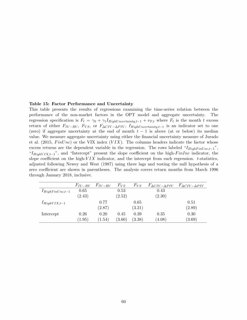
Table 15: Factor Performance and UncertaintyThis table presents the results of regressions examining the time-series relation between theperformance of the non-market factors in the OPT model and aggregate uncertainty. Theregression specification is Ft = γ0 + γ1IHighUncertainty,t−1 + νF,t where Ft is the month t excessreturn of either FIV−RV , FV S , or F∆CIV−∆PIV , IHighUncertainty,t−1 is an indicator set to one(zero) if aggregate uncertainty at the end of month t − 1 is above (at or below) its medianvalue. We measure aggregate uncertainty using either the financial uncertainty measure of Juradoet al. (2015, FinUnc) or the VIX index (V IX). The columns headers indicate the factor whoseexcess returns are the dependent variable in the regression. The rows labeled “IHighFinUnc,t−1”,“IHighV IX,t−1”, and “Intercept” present the slope coefficient on the high-FinInc indicator, theslope coefficient on the high-V IX indicator, and the intercept from each regression. t-statistics,adjusted following Newey and West (1987) using three lags and testing the null hypothesis of azero coefficient are shown in parentheses. The analysis covers return months from March 1996through January 2018, inclusive.

FIV−RV FIV−RV FV S FV S F∆CIV−∆PIV F∆CIV−∆PIV

IHighFinUnc,t−1 0.65 0.53 0.43(2.43) (2.52) (2.30)

IHighV IX,t−1 0.77 0.65 0.51(2.87) (3.21) (2.89)

Intercept 0.26 0.20 0.45 0.39 0.35 0.30(1.95) (1.54) (3.60) (3.38) (4.08) (3.69)

60

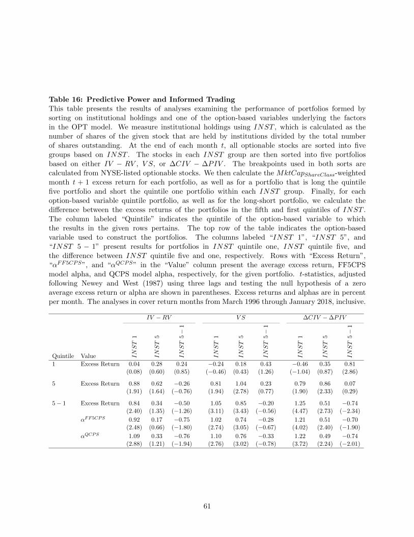
Table 16: Predictive Power and Informed TradingThis table presents the results of analyses examining the performance of portfolios formed bysorting on institutional holdings and one of the option-based variables underlying the factorsin the OPT model. We measure institutional holdings using INST , which is calculated as thenumber of shares of the given stock that are held by institutions divided by the total numberof shares outstanding. At the end of each month t, all optionable stocks are sorted into fivegroups based on INST . The stocks in each INST group are then sorted into five portfoliosbased on either IV − RV , V S, or ∆CIV − ∆PIV . The breakpoints used in both sorts arecalculated from NYSE-listed optionable stocks. We then calculate the MktCapShareClass-weightedmonth t + 1 excess return for each portfolio, as well as for a portfolio that is long the quintilefive portfolio and short the quintile one portfolio within each INST group. Finally, for eachoption-based variable quintile portfolio, as well as for the long-short portfolio, we calculate thedifference between the excess returns of the portfolios in the fifth and first quintiles of INST .The column labeled “Quintile” indicates the quintile of the option-based variable to whichthe results in the given rows pertains. The top row of the table indicates the option-basedvariable used to construct the portfolios. The columns labeled “INST 1”, “INST 5”, and“INST 5 − 1” present results for portfolios in INST quintile one, INST quintile five, andthe difference between INST quintile five and one, respectively. Rows with “Excess Return”,“αFF5CPS”, and “αQCPS” in the “Value” column present the average excess return, FF5CPSmodel alpha, and QCPS model alpha, respectively, for the given portfolio. t-statistics, adjustedfollowing Newey and West (1987) using three lags and testing the null hypothesis of a zeroaverage excess return or alpha are shown in parentheses. Excess returns and alphas are in percentper month. The analyses in cover return months from March 1996 through January 2018, inclusive.

IV −RV V S ∆CIV −∆PIV

Quintile Value INST

1

INST

5

INST

5−

1

INST

1

INST

5

INST

5−

1

INST

1

INST

5

INST

5−

1

1 Excess Return 0.04 0.28 0.24 −0.24 0.18 0.43 −0.46 0.35 0.81(0.08) (0.60) (0.85) (−0.46) (0.43) (1.26) (−1.04) (0.87) (2.86)

5 Excess Return 0.88 0.62 −0.26 0.81 1.04 0.23 0.79 0.86 0.07(1.91) (1.64) (−0.76) (1.94) (2.78) (0.77) (1.90) (2.33) (0.29)

5− 1 Excess Return 0.84 0.34 −0.50 1.05 0.85 −0.20 1.25 0.51 −0.74(2.40) (1.35) (−1.26) (3.11) (3.43) (−0.56) (4.47) (2.73) (−2.34)

αFF5CPS 0.92 0.17 −0.75 1.02 0.74 −0.28 1.21 0.51 −0.70(2.48) (0.66) (−1.80) (2.74) (3.05) (−0.67) (4.02) (2.40) (−1.90)

αQCPS 1.09 0.33 −0.76 1.10 0.76 −0.33 1.22 0.49 −0.74(2.88) (1.21) (−1.94) (2.76) (3.02) (−0.78) (3.72) (2.24) (−2.01)

61

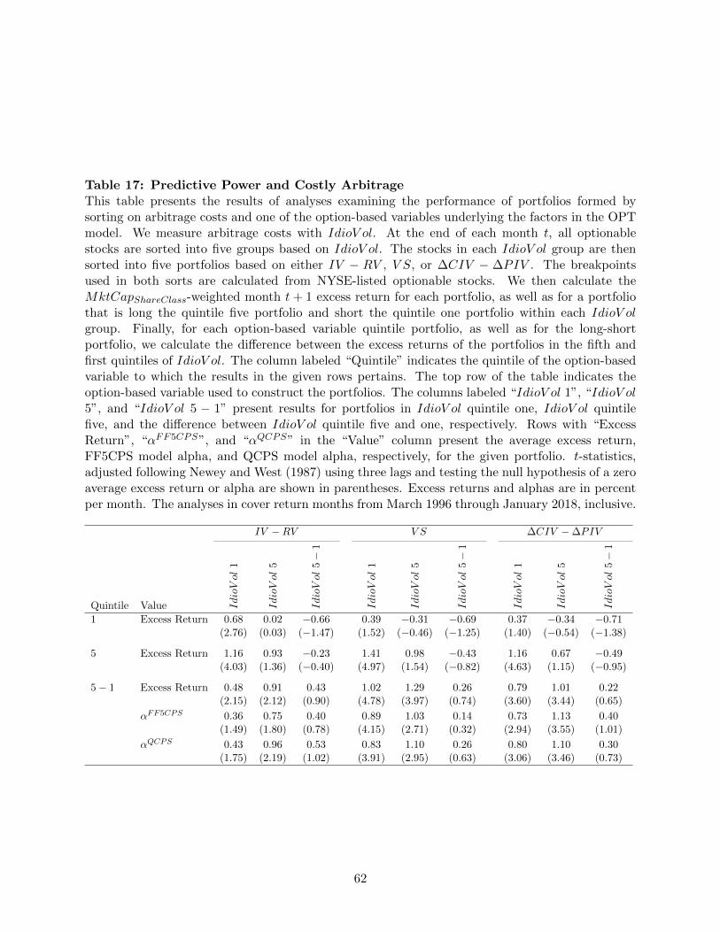
Table 17: Predictive Power and Costly ArbitrageThis table presents the results of analyses examining the performance of portfolios formed bysorting on arbitrage costs and one of the option-based variables underlying the factors in the OPTmodel. We measure arbitrage costs with IdioV ol. At the end of each month t, all optionablestocks are sorted into five groups based on IdioV ol. The stocks in each IdioV ol group are thensorted into five portfolios based on either IV − RV , V S, or ∆CIV − ∆PIV . The breakpointsused in both sorts are calculated from NYSE-listed optionable stocks. We then calculate theMktCapShareClass-weighted month t+ 1 excess return for each portfolio, as well as for a portfoliothat is long the quintile five portfolio and short the quintile one portfolio within each IdioV olgroup. Finally, for each option-based variable quintile portfolio, as well as for the long-shortportfolio, we calculate the difference between the excess returns of the portfolios in the fifth andfirst quintiles of IdioV ol. The column labeled “Quintile” indicates the quintile of the option-basedvariable to which the results in the given rows pertains. The top row of the table indicates theoption-based variable used to construct the portfolios. The columns labeled “IdioV ol 1”, “IdioV ol5”, and “IdioV ol 5 − 1” present results for portfolios in IdioV ol quintile one, IdioV ol quintilefive, and the difference between IdioV ol quintile five and one, respectively. Rows with “ExcessReturn”, “αFF5CPS”, and “αQCPS” in the “Value” column present the average excess return,FF5CPS model alpha, and QCPS model alpha, respectively, for the given portfolio. t-statistics,adjusted following Newey and West (1987) using three lags and testing the null hypothesis of a zeroaverage excess return or alpha are shown in parentheses. Excess returns and alphas are in percentper month. The analyses in cover return months from March 1996 through January 2018, inclusive.

IV −RV V S ∆CIV −∆PIV

Quintile Value IdioVol

1

IdioVol

5

IdioVol

5−

1

IdioVol

1

IdioVol

5

IdioVol

5−

1

IdioVol

1

IdioVol

5

IdioVol

5−

11 Excess Return 0.68 0.02 −0.66 0.39 −0.31 −0.69 0.37 −0.34 −0.71

(2.76) (0.03) (−1.47) (1.52) (−0.46) (−1.25) (1.40) (−0.54) (−1.38)

5 Excess Return 1.16 0.93 −0.23 1.41 0.98 −0.43 1.16 0.67 −0.49(4.03) (1.36) (−0.40) (4.97) (1.54) (−0.82) (4.63) (1.15) (−0.95)

5− 1 Excess Return 0.48 0.91 0.43 1.02 1.29 0.26 0.79 1.01 0.22(2.15) (2.12) (0.90) (4.78) (3.97) (0.74) (3.60) (3.44) (0.65)

αFF5CPS 0.36 0.75 0.40 0.89 1.03 0.14 0.73 1.13 0.40(1.49) (1.80) (0.78) (4.15) (2.71) (0.32) (2.94) (3.55) (1.01)

αQCPS 0.43 0.96 0.53 0.83 1.10 0.26 0.80 1.10 0.30(1.75) (2.19) (1.02) (3.91) (2.95) (0.63) (3.06) (3.46) (0.73)

62