in school and out of trouble? the minimum dropout age and

1

In School and Out of Trouble? The Minimum Dropout Age and Juvenile Crime

D. Mark Anderson Department of Economics

University of Washington

[email protected]

November 2009

Abstract

Does increasing the minimum dropout age reduce juvenile crime rates? Despite popular

accounts that link school attendance to keeping youth out of trouble, little systematic research

has analyzed the contemporaneous relationship between schooling and juvenile crime. This

paper examines the connection between the minimum age at which youth can legally dropout of

high school and juvenile arrest rates by exploiting state-level variation in the minimum dropout

age. Using county-level arrest data for the U.S. between 1980 and 2006, a difference-in-

difference-in-difference empirical strategy compares the arrest behavior over time of various age

groups within counties that differ by their state‟s minimum dropout age. The evidence suggests

that minimum dropout age requirements have a significant and negative effect on property and

violent crime arrest rates for youth aged 16 to 18 years-old, and these estimates are robust to a

range of specification checks. Furthermore, the results are consistent with an incapacitation

effect; school attendance decreases the time available for criminal activity. Not only do these

findings provide support for the efficacy of programs intended to keep youth in school and out of

delinquency, but this information is likely to be of value to policy-makers deciding on whether or

not to increase their state‟s minimum dropout age.

Keywords: Minimum dropout age; Juvenile crime; Delinquency

JEL classification: H75; I20; I28; K42

I am grateful to Claus Portner for his guidance. I owe thanks to Yoram Barzel, Shawn Bushway, Andy Hanssen,

Lars Lefgren, Lance Lochner, Shelly Lundberg, Lan Shi, Wendy Stock, Chris Stoddard, Edwin Wong and seminar

participants at the University of Washington for comments and suggestions. I also owe a special thanks to Philip

Oreopoulos for providing data on compulsory schooling laws and Thomas Dee for providing data on minimum legal

drinking ages. All remaining errors and omissions in this paper are solely mine.

mailto:[email protected]

2

“Dropout prevention is crime prevention.”

Los Angeles County Sheriff Lee Baca

I. Introduction

Does increasing the minimum age at which youth are legally permitted to leave school

keep them off the streets and away from crime? Previous research suggests a correlation

between youth dropouts and juvenile criminal behavior (see, e.g., Thornberry et al. 1985; Fagan

and Pabon 1990). In California, it has been estimated that dropouts are responsible for 1.1

billion dollars in annual juvenile crime costs (Belfield and Levin 2009). Because of crime‟s

deleterious consequences, it is important to understand whether or not being in school has a

causal influence on juvenile offending; evidence proposes that involvement in juvenile crime

adversely impacts economic outcomes later in life. Incarceration is associated with lower

educational attainment and decreased future earnings (Hjalmarsson 2008; Waldfogel 1994a;

Waldfogel 1994b; Western 2002). Juvenile crime not only has an immediate impact on the

delinquent and their victim(s), but can impose negative externalities on those not directly

involved with criminal acts (see, e.g., Grogger 1997).

Previous studies have focused on a wide array of determinants of juvenile crime. In

general, much of the literature has concentrated on deterrence and punishment as crime-reducing

mechanisms.1 Research has also documented the impact of wages (Hashimoto 1987; Grogger

1998), high school experience (Arum and Beattie 1999), youth employment (Apel et al. 2008),

underage drinking (French and Maclean 2006), and curfew ordinances (Kline 2009) to name a

few.

1 See, e.g., Becker (1968), Corman and Mocan (2000), Di Tella and Schargrodsky (2004), Freeman (1996),

Friedman (1999), and Levitt (1997, 1998).

3

This paper joins the sparse, yet growing, literature on the effects of education on crime by

investigating the relationship between the minimum dropout age (MDA) and juvenile arrest

rates. Little research has been devoted to studying the contemporaneous relationship between

schooling and crime. Most of the previous work has focused on proxies for educational

attainment and subsequent criminal behavior. Empirical research in this area, however, is not

decisive. Tauchen et al. (1994) and Witte and Tauchen (1994) find that having a parochial

school education is significantly associated with lower criminal behavior, but that a high school

degree has no significant effect. Grogger‟s (1998) results indicate that having additional years

of education or a high school diploma do not have a significant effect on criminal activity. On

the other hand, Lochner (2004) and Lochner and Moretti (2004) estimate a negative effect of

education on property and violent crimes.

More closely related to this paper, other research has studied the connection between time

spent at school and criminal activity. Farrington et al. (1986), Gottfredson (1985), and Witte and

Tauchen (1994) find that time spent at school is associated with lower levels of criminal

behavior. However, these studies do not control for the potential endogeneity of schooling. Two

recent papers have explicitly studied the incapacitation and concentration effects of school

attendance.2 An incapacitation effect of school is that it keeps juveniles occupied, leaving less

time and opportunity to commit crimes. However, forcing children to stay in school increases

the concentration of juveniles and, thus, the number of interactions that facilitate delinquency.

Jacob and Lefgren (2003) examine the impact of school attendance on crime by exploiting

variation in teacher in-service days. Luallen (2006) uses teacher strikes as a source of variation

in student attendance. Both papers find that property crimes committed by juveniles decrease

2 The incapacitation function of criminal sanctions is to prevent individuals from doing harm to society by removing

them from the population (Shavell 1987).

4

significantly when school is in session, but violent juvenile crime rates increase on these days.

In related research, Aizer (2004) finds that children with adult supervision are less likely to

participate in delinquent behavior. Her results suggest that after-school programs geared to

engage school-age children may decrease delinquency and have important implications for their

development of human capital and future earnings.

Using a difference-in-difference-in-difference (DDD) estimation strategy, this paper

exploits the variation in compulsory schooling laws, across states over time, to find strong

evidence that increases in the minimum dropout age reduce incidences of property and violent

crime arrests among high school-aged youth. The magnitude of the negative effect is greater

when the sample is restricted to “black” counties. Robustness checks help to confirm the results

are not driven by omitted state-specific characteristics. These findings suggest that policy

interventions to keep kids in school may be successful at decreasing juvenile crime.

Besides being one of the few papers to explore the contemporaneous link between

schooling and crime, this paper distinguishes itself from previous research by attempting to

understand the underlying factors that drive this relationship. Several possible mechanisms are

discussed. First, the incapacitation effect is considered. To the extent that being in school

reduces the time available for delinquent activity, we might expect an increase in the minimum

dropout age to negatively influence criminal behavior. Second, those compelled by law to

remain in school longer may build important human capital that decreases their relative returns to

crime. Lastly, spillover effects that influence youth slightly above the minimum dropout age

may also impact delinquency. These mechanisms are discussed in further detail in Section VI.

The results favor an incapacitation effect, but possible spillovers also appear important.

5

The remainder of the paper is organized as follows: Section II discusses the background

of compulsory schooling laws, relevant literature, and empirical evidence concerning the

relationship between compulsory schooling and attendance; Section III describes the data;

Section IV lays out the empirical identification strategy; Section V discusses the results; Section

VI attempts to understand the causal relationship between schooling and crime; Section VII

concludes.

II. Compulsory Schooling Laws

Background of Compulsory Schooling Laws

In 1852, Massachusetts was the first state to enact a compulsory schooling law. By 1918,

all states had a law in place (Lleras-Muney 2002). In general, these laws specify a minimum and

maximum age for which attendance is required. Historically, compulsory schooling laws have

changed frequently across states. Table 1 illustrates there has been a strong movement towards

increasing the minimum dropout age in recent years. For example, Illinois and Indiana have

recently increased their minimum dropout age from 16 to 17 and 18, respectively. However,

there are also states that have maintained a constant minimum dropout age for over the past 50

years. Iowa, Michigan, and Montana have had a leaving age of 16 during this period, while

Ohio, Oklahoma, and Utah have maintained an age of 18. In addition, several states have raised

and lowered their minimum dropout age across the period.

Not surprisingly, compulsory schooling legislation is more complex than simply

specifying a mandatory leaving age. Some states allow exemptions if the child is working or has

obtained parental consent. States also vary in their degrees of punishing truancy. Additionally,

6

it is not uncommon for a state to punish the parents of a truant child. See Oreopoulos (2008) for

a more complete discussion of state-by-state legislation.3

Relevant Literature

Previous research has focused on compulsory schooling legislation to estimate the returns

to education. Acemoglu and Angrist (2001) instrument educational attainment with compulsory

schooling laws and school entry to find that the individual returns to compulsory schooling are

approximately 8 percent. Oreopoulos (2006) uses a regression discontinuity design and

compares local average treatment effects estimates for North America to the U.K. His

conclusion is that the gains from compulsory attendance are substantial whether the laws impact

a majority or minority of the school-aged population. For Canada, Oreopoulos (2006) finds that

an extra year of mandated education is associated with an increase in average annual income by

about 12 percent. In a theoretical treatment, Eckstein and Zilcha (1994) present an overlapping

generations model where parents under invest in their children‟s education because they do not

consider the external effect on the aggregate production function. They show that in the long run

the majority of the population can be made better off when compulsory attendance is

implemented.

In other applications of compulsory attendance, Black et al. (2008) examine whether

increasing mandatory schooling causes females to postpone having children. They find that

minimum school requirements have a significant and negative effect on the probability of having

a child as a teenager. Lleras-Muney (2005) uses compulsory schooling laws as an instrumental

variable to show that education has a negative effect on mortality. Closely related to this study,

Lochner and Moretti (2004) estimate the effect of educational attainment on criminal activity

3 In particular, Table 1 in Oreopoulos (2008) lists examples of exemptions and punishments for states with a

minimum dropout age greater than 16.

7

later in life using the variation in state compulsory schooling laws to instrument endogenous

schooling decisions. It is important to note, these studies focus on the number of years of

mandatory schooling as opposed to the minimum dropout age. Though positively correlated, a

higher minimum dropout age does not necessarily mean more years of compulsory schooling

because states also differ in their mandatory starting age. For example, Oregon and Maryland

both require 12 years of compulsory schooling; yet, the minimum dropout ages for Oregon and

Maryland are 18 and 16, respectively. Because this paper‟s attention is on the contemporaneous

relationship between being in school and crime, the minimum dropout age is the variable of

interest.

Compulsory Schooling and Attendance: Empirical Evidence

This study is concerned with the reduced form relationship between compulsory

schooling laws and juvenile crime. Implicit to this relationship is that compulsory schooling

laws are effective at impacting attendance rates. Previous research is in accordance with this

assumption. Angrist and Krueger (1991) find that approximately 25% of potential dropouts in

the U.S. remain in school because of compulsory schooling laws. Wenger (2002) illustrates that

increasing a state‟s dropout age is consistently predicted to decrease the probability that an

individual will drop out of high school. More specifically, she finds the change in probability is

equivalent to a decrease in the dropout rate of roughly sixteen percent. The results in

Oreopoulos (2008) also suggest that more restrictive compulsory schooling laws have reduced

dropout rates. Using less recent data, Lleras-Muney (2002) provides strong evidence that school

leaving laws were responsible for increased attendance from 1915 to 1939.

As pointed out by Angrist and Krueger (1991), the efficacy of compulsory schooling

legislation is likely due to two enforcement mechanisms. In a majority of states, children are not

8

permitted to work during school hours unless they are of the state‟s compulsory schooling age.

Additionally, young workers are required to obtain work permits that are often granted by school

administrators. This, to an extent, allows schools to monitor the behavior of youth who are

below the minimum dropout age. Consider, it is possible the fraction of dropouts who seek

employment are less likely to commit crimes than the youth who dropout and have no interest in

working. For the latter individuals, direct enforcement and policing may be more effective

means of mandating attendance. More specifically, state legislation provides truancy officers to

enforce the law; officers are given the authority to arrest truant youth without a warrant.

Truancy regulations are also enforced by school officials and, as mentioned, are often

implemented under the context of parental responsibility.

III. Data

The juvenile arrest data come from the FBI‟s Uniform Crime Reports (UCR).4 These

data are aggregated by the age of the offender at the county-level for the period 1980-2006.5

Arrest rates are arrests per 1,000 people of the specified age group.6 Arrests are reported for

violent crimes (aggravated assault and robbery), property crimes (auto theft, larceny, and

burglary) and drug related crimes (selling and possession). The violent, property, and drug crime

indices represent unweighted aggregations of their respective individual components. The

decision to exclude rape and murder from the violent crime index was made because these

4 U.S. Department of Justice, FBI, Uniform Crime Reports: Arrests by Age, Sex, and Race. Washington, DC: U.S.

Department of Justice, FBI; Ann Arbor, MI: Inter-university Consortium for Political and Social Research (ICPSR,

distributor). 5 Data for the year 1984 were unavailable from the ICPSR.

6 These rates were calculated using the National Cancer Institute, Surveillance Epidemiology and End Results, U.S.

Population Data.

9

crimes account for a very small fraction of juvenile violent crime. This paper analyzes male

arrest rates.

Collection of the arrest data was completed through a cooperative effort of self-reporting

by more than 16,000 city, county, and state law enforcement agencies. Of course, with a project

of this magnitude, there are reasons to be cautious of the self-reported data. Gould et al. (2002)

point out that measurement error in the arrest rates can exist because not every crime committed

is reported to the police. Additionally, under-reporting can vary by crime type or county of

jurisdiction. Data collection and reporting methods may vary by jurisdiction as well.

Fortunately, county-fixed effects eliminate the impact of time-invariant, cross-county differences

in data collection and reporting techniques.

It is important to note that arrests, as opposed to the actual number of offenses

committed, are used as the measure of criminal activity. The primary reason for using arrest

rates is that detailed age data are not available in the UCR offense reports. Although arrests are

not a perfect measure of youth criminal behavior and likely understate the true level of crime,

other research indicates that arrest data serve as an accurate representation of underlying criminal

activity.7 Furthermore, this type of measurement error is unlikely correlated with the minimum

dropout age. Using the UCR data, Lochner and Moretti (2004) report the correlation between

arrests and crimes committed to be very high.8

Following Gould et al. (2002), this paper restricts the sample to all counties with an

average population exceeding 25,000 between 1980 and 2006. This selection criterion is

intended to capture a representative population and eliminate counties where arrest reports are

more likely to be inaccurate. In addition, counties with less than 13 out of 26 complete years of

7 See, e.g., Hindelang (1978, 1981).

8 0.96 for rape and robbery, 0.94 for murder, assault, and burglary, and 0.93 for auto theft.

10

data are omitted from the sample. Alaskan and Hawaiian counties are also excluded because of

their significantly different demographics and economies. Finally, all counties in Mississippi are

dropped because Mississippi was the only state during the sample time frame to have a minimum

dropout age less than 16. The decision to drop Mississippi was made because the control group,

described in detail below, consists of youth below the age of 16. The results, however, change

little when Mississippi counties are included in the analysis.

County-level demographic variables come from the U.S. Census Bureau. The regressions

control for the county population density, the percentage of the county population that was black,

the percentage that was male, and the percentages in the age ranges 10-19, 20-29, 30-39, 40-49,

50-64, and 65 plus. Data on real per capita personal income and the average annual wage of jobs

covered by unemployment insurance come from the Bureau of Economic Analysis. The per

capita income and wage variables are deflated by the Consumer Price Index to convert to 2000

dollars. Variables indicating each state‟s minimum legal drinking age across each year of the

period under study were provided by Dee (2001). The state-by-state minimum dropout ages

come from Oreopoulos (2008) and the National Center for Education Statistics‟ Digest of

Education Statistics.

Table 2 presents descriptive statistics for all counties in the sample. Table 3 provides a

breakdown of the mean arrest rates for 16, 17, and 18 year-olds by their county‟s prevailing

minimum dropout law. For property and violent crimes, the highest arrest rates are shown for

counties with a minimum dropout age of 16. Across age cohorts, property crime arrest rates

appear lowest for 16 year-olds, while 17 and 18 year-olds appear to commit property crimes at

comparable rates. Violent crime arrest rates increase with age. The highest rate of property

crime arrests and violent crime arrests can be attributed to 17 year-olds in counties with a

11

minimum dropout age of 16 and 18 year-olds in counties with a minimum dropout age of 16,

respectively. Drug sale arrests are most prevalent among 18 year-olds in counties with a leaving

age of 16, while drug possession arrests are greatest for 18 year-olds in counties with a leaving

age of 18.

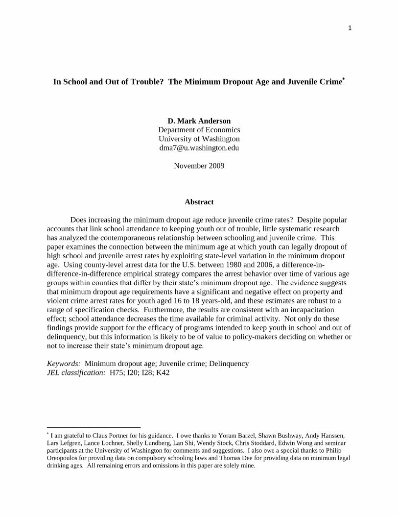
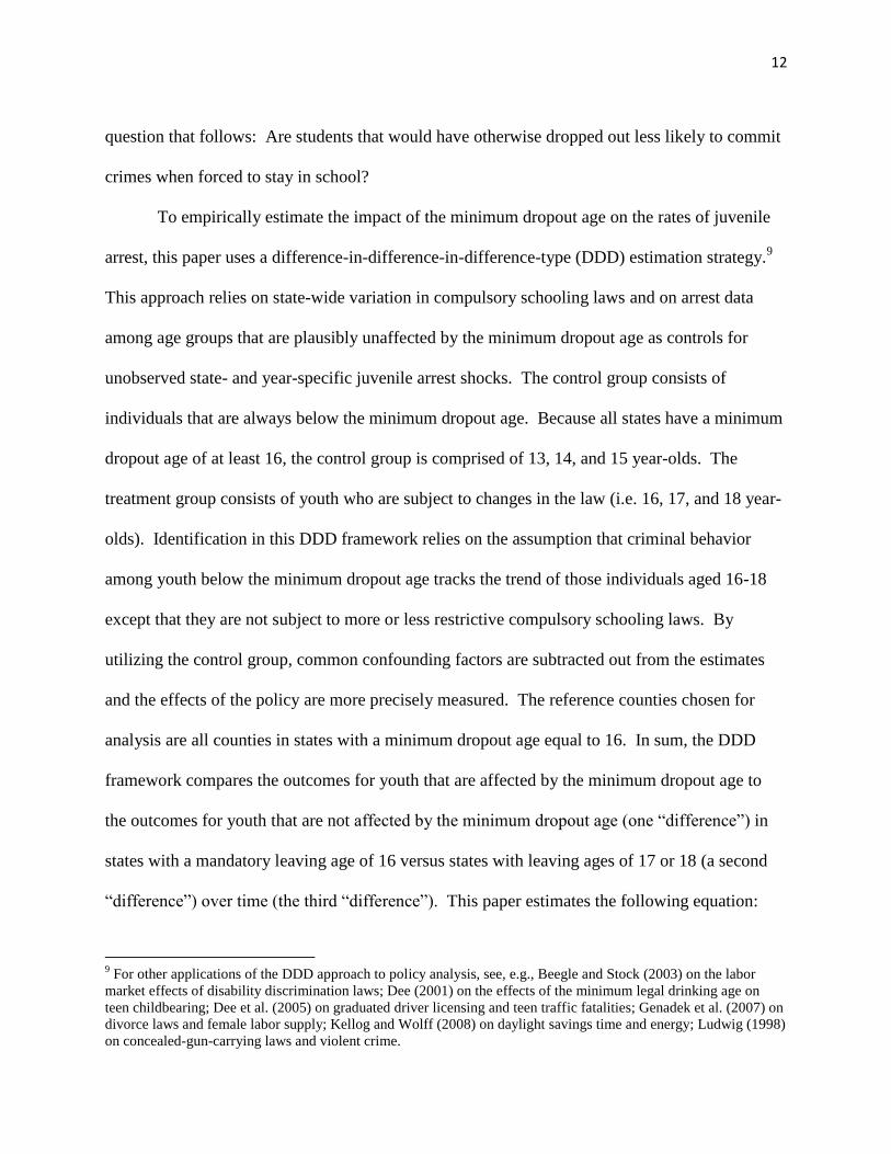
Figures 1 and 2 illustrate the relationship between the average minimum dropout age for

states in the sample and the rates of property crime and violent crime among 16, 17, and 18 year-

olds, respectively. Figure 1 shows a substantial fall in the rates of property crime arrests after the

early „90s. During this same period, the average minimum dropout age was steadily increasing.

In the mid „80s, when the average minimum dropout age was fairly constant, the property crime

rates showed little change. Figure 2, on the other hand, provides less confirmation that the

mandatory leaving age has an impact on violent crime. As with property crime, violent crime

arrest rates decreased from the early „90s onward when the average minimum dropout age was

increasing. Unlike property crimes, violent crime arrests increased drastically from the late „80s

until about 1992. Because these crime trends were experienced by most regions in the U.S., it is

more nearly appropriate to compare the magnitude of the changes between counties with

differing minimum dropout ages. In addition, these data also suggest that it is important to

control for preexisting trends. These concerns are dealt with in the analysis that follows.

IV. Empirical Identification

As mentioned, this study aims to evaluate the impact of the minimum dropout age on

juvenile arrest rates by exploiting variation in state-level compulsory schooling laws. One

expects to observe a higher percentage of 16 and 17 year-olds attending school in states with

minimum dropout ages of 18 when compared to states with a leaving age of 16 or 17. The

12

question that follows: Are students that would have otherwise dropped out less likely to commit

crimes when forced to stay in school?

To empirically estimate the impact of the minimum dropout age on the rates of juvenile

arrest, this paper uses a difference-in-difference-in-difference-type (DDD) estimation strategy.9

This approach relies on state-wide variation in compulsory schooling laws and on arrest data

among age groups that are plausibly unaffected by the minimum dropout age as controls for

unobserved state- and year-specific juvenile arrest shocks. The control group consists of

individuals that are always below the minimum dropout age. Because all states have a minimum

dropout age of at least 16, the control group is comprised of 13, 14, and 15 year-olds. The

treatment group consists of youth who are subject to changes in the law (i.e. 16, 17, and 18 year-

olds). Identification in this DDD framework relies on the assumption that criminal behavior

among youth below the minimum dropout age tracks the trend of those individuals aged 16-18

except that they are not subject to more or less restrictive compulsory schooling laws. By

utilizing the control group, common confounding factors are subtracted out from the estimates

and the effects of the policy are more precisely measured. The reference counties chosen for

analysis are all counties in states with a minimum dropout age equal to 16. In sum, the DDD

framework compares the outcomes for youth that are affected by the minimum dropout age to

the outcomes for youth that are not affected by the minimum dropout age (one “difference”) in

states with a mandatory leaving age of 16 versus states with leaving ages of 17 or 18 (a second

“difference”) over time (the third “difference”). This paper estimates the following equation:

9 For other applications of the DDD approach to policy analysis, see, e.g., Beegle and Stock (2003) on the labor

market effects of disability discrimination laws; Dee (2001) on the effects of the minimum legal drinking age on

teen childbearing; Dee et al. (2005) on graduated driver licensing and teen traffic fatalities; Genadek et al. (2007) on

divorce laws and female labor supply; Kellog and Wolff (2008) on daylight savings time and energy; Ludwig (1998)

on concealed-gun-carrying laws and violent crime.

13

1 st 2 st 3 i 4 i 5 i

6 st i 7 st i 8 st i

9 st i 10 st i 11 st i

12 13 14 15

MDA17 MDA18 age16 age17 age18

(MDA17 age16 ) (MDA17 age17 ) (MDA17 age18 )

(MDA18 age16 ) (MDA18 age17 ) (MDA18 age18 )

ijstY

jst j t

+

+ + +

+X C T Trend ijst

(1)

where i indexes the age cohort, j indexes the county, s indexes the state, and t indexes the year.

In equation (1), MDA17 and MDA18 are equal to one if the state has a minimum dropout

age of 17 or 18, respectively, and equal to zero otherwise. The variables age16, age17, and

age18 are dummy variables that control for differences in age groups that are common across

years. X is a vector of the county- and state-level controls as described above. C represents

county fixed effects and T represents time fixed effects. The county fixed effects control for

differences in counties that are common across years, while the time fixed effects control for

differences across time that are common to individuals of all ages and all counties. Lastly,

Trend represents linear state-specific time trends that account for time-series variations within

each state.

The interaction term coefficients, β6, β7, β8, β9, β10, β11, represent the difference-in-

difference-in-difference-type estimates of the effects of minimum dropout ages on juvenile arrest

rates. More specifically, these coefficients measure the differential impacts of compulsory

schooling legislation on youth 16, 17, and 18 years of age. If increases in compulsory schooling

decreases crime among youth 16 to 18 years of age, then we expect the coefficients β6 through

β11 to be negative. If increasing the dropout age only impacts youth of ages where the law binds,

then we expect only β6, β9, and β10 to be negative. In describing the incapacitation effect, Section

VI discusses why we might expect only β6, β9, and β10 to be negative.

14

The DDD approach addresses at least three important endogeneity problems. First, there

is a strong association between age and crime rates. As a result, comparing the criminal behavior

of 16-18 year-olds to 13-15 year-olds raises some concerns. However, the DDD estimator

alleviates this issue because it also compares arrest rates of 16-18 year-olds in states with a

mandatory leaving age of 17 or 18 to arrest rates of 16-18 year-olds in states with a leaving age

of 16. Second, expectations of when a student will be able to dropout may influence current

criminal behavior. For example, a 16 year-old in a state with a minimum dropout age of 17 may

behave differently than a 16 year-old in a state with a minimum dropout age of 18 because the

former anticipates being able to dropout sooner. Again, the DDD estimator mitigates these

concerns because it compares youth of different ages within states that have similar mandatory

leaving ages. Lastly, the DDD technique controls for the potential endogeneity of the

compulsory schooling laws. This is accomplished by differencing over time. That is, the DDD

estimator examines changes in arrest rates, as opposed to differences in levels. As a result,

permanent differences in the characteristics of states are taken into account.10

All DDD models are estimated with weighted least squares where mean county

populations are used as weights. Following Bertrand et al. (2004), standard errors are clustered

at the state-level. This procedure accounts for the possibility that standard errors may be biased

due to serial correlations of the policy variables over time within a state.

10

Another concern is that the minimum dropout age is associated with police enforcement. However, Lochner and

Moretti (2004) find little evidence that compulsory schooling legislation is correlated with police expenditures or the

number of policemen.

15

V. Results

Before proceeding to the DDD regression results, Table 4 summarizes the mean

differences of arrest rates by minimum dropout age laws and age group. Table 4 restricts focus

to arrest rates for MDA = 16 and MDA = 18 counties. For a comparison of MDA = 16 to MDA

= 17 counties and MDA = 17 to MDA = 18 counties, see Tables A1 and A2, respectively, in the

Appendix. For the treatment group, that is, youth who are 16 to 18 years of age, the mean total

crime arrest rate is approximately 6.2 arrests lower per 1,000 of the age cohort population in

MDA = 18 counties as opposed to MDA = 16 counties. For property and violent crimes, the

arrest rates are roughly 3.8 and 2.5 arrests per 1,000 lower, respectively, in MDA = 18 counties.

These are statistically significant changes. The control group shows that 13 to 15 year-olds

actually have a higher mean property crime arrest rate in MDA = 18 counties. Violent crime

arrest rates for the control group are essentially the same across county-type. Subtracting the

MDA = 16 and MDA = 18 difference in the control group from the MDA = 16 and MDA = 18

difference in the treatment group shows property crimes are lower by approximately 7.7 arrests

per 1,000 and violent crimes are lower by roughly 2.4 arrests per 1,000.

Figure 3 illustrates the relationship between increases in compulsory schooling and arrest

rates over time. The plotted points represent the estimated coefficients on lead and lag indicators

for whether total crime arrest rates of 16 to 18 year-olds decrease after an increase in the MDA in

a regression that controls for age, county, and year effects.11

Time zero stands for the year the

laws were reformed. This figure demonstrates a relatively discrete change in arrest behavior

around the changes in the minimum dropout age and suggests that increasing the minimum

dropout age is associated with lower arrest rates for 16 to 18 year-olds.

11

This figure only documents counties in states that changed from an MDA = 16 to an MDA = 18.

16

Total Crime Arrest Rates

Table 5 presents the DDD estimates from equation (1). The coefficients illustrated are

those of the interaction terms between the minimum dropout age indicators and the age cohort

dummies. Each column of Table 5 represents separate regression results where the total crime

arrest rate is the dependent variable (i.e. property crimes plus violent crimes). The estimates in

Column 1 compare arrest rates for counties in states with a minimum dropout age of 16 to all

other counties. The approach taken in Column 2, and throughout the remainder of the paper,

allows for differences between counties in MDA = 17 and MDA = 18 states. This latter

specification is preferred because one expects leaving ages of 16 and 17 to impact youth

differently. Column 1 indicates that being in a state with a mandatory leaving age of 16 is

associated with statistically significant and higher arrest rates for 16 and 17 year-olds. For 16

year-olds, the coefficient estimate indicates a higher rate of crime by approximately 5 incidences

per 1,000 of the age cohort population. This estimate increases to nearly 6.6 more incidences per

1,000 for 17 year-olds. In Column 2, movement away from a minimum dropout age of 16 to

leaving ages of 17 and 18 is associated with decreases in the arrest rate. Here, all coefficient

estimates are negative with results for 17 year-olds in MDA = 17 states and 16 and 17 year-olds

in MDA = 18 states being statistically significant at the 5% level. For example, movement to a

mandatory leaving age of 18 reduces total crime arrest rates for 16 and 17 year-olds by roughly

5.8 and 7.4 incidences per 1,000 of the age cohort population, respectively. To put these

estimates into further perspective, this represents a 9.7% decrease from the mean rate of total

crime arrests for 16 year-olds in MDA = 16 states and an 11.5% decrease from the mean for 17

year-olds in MDA = 16 states.

17

Arrest Rates by Types of Offenses

Table 6 breaks down total crime into property and violent crimes and their respective

components. In addition, drug crime arrests are reported and separated into arrests associated

with the selling of drugs and arrests associated with the possession of drugs.

The estimates in Table 6 suggest that increasing the minimum dropout age has a negative

impact on property and violent crime. For example, the results in Column 1 indicate that the

movement to a minimum dropout age of 18 reduces property crime arrests by approximately 3.5

and 4.6 incidences per 1,000 of the age cohort population for 16 and 17 year-olds, respectively.

These numbers represent roughly a 6.9% reduction from the mean rate of property crime for 16

year-olds in MDA = 16 states and about an 8.7% reduction from the mean for 17 year-olds in

these same states. In Column 1, all coefficients are negative in sign, while results for 16 and 17

year-olds in MDA = 18 states are significant. The coefficient estimates for 16 and 17 year-olds

in MDA = 17 states are slightly smaller in magnitude than the estimates for similar aged youth in

MDA = 18 states, however, these estimates are not significant at conventional levels.

For the individual property crime offenses, all coefficient estimates suggest a negative

relationship between the minimum dropout age and the rate of juvenile arrest with the exception

of the auto theft and larceny estimates for 18 year-olds in MDA = 17 states. Here, the point

estimates are positive, but small in magnitude suggesting little difference in the impact of a

leaving age of 16 or 17 for an 18 year-old. This is unsurprising given that the choice to dropout

for an 18 year-old is equally unconstrained in either type of state. In Column 3, movement to a

minimum dropout age of 18 reduces larceny arrests among 17 year-olds by approximately 2.6

incidences per 1,000 of the age cohort population. This represents roughly an 8.3% reduction

from the mean rate of larceny for 17 year-olds in MDA = 16 states. For burglary, a leaving age

18

of 18 is associated with a reduction in arrests from the mean by approximately 11% and 10% for

16 and 17 year-olds, respectively. The result for 17 year-olds, however, is only weakly

significant at the 10% level. The statistically insignificant effects of exposure to a minimum

dropout age of 17 are not completely surprising because the sample variation in an MDA of 17

was limited relative to an MDA of 18.

Similar to property crime, all of the interaction term coefficient estimates are negative in

the violent crime regression. For 17 year-olds, movement to an MDA = 17 reduces violent crime

arrests by approximately 2.3 incidences per 1,000; an MDA = 18 reduces violent crime arrests

among this age group by approximately 2.7 incidences per 1,000. These figures represent

reductions of roughly 21% and 25%, respectively, from the mean rates of 17 year-olds in MDA =

16 states. Coefficient estimates for 16 year-olds are negative and large in magnitude, but not

significant at conventional levels. Interestingly, results for 18 year-olds are significant, albeit at

the 10% level. One would initially not expect a minimum dropout age of 17 to impact an 18

year-old differently than a minimum dropout age of 16. In each case, an 18 year-old is free to

dropout if he so chooses. Perhaps the most reasonable explanation is that forcing a student to

attend school one more year increases the likelihood the student will finish high school. This

suggestion is supported by the aforementioned literature on the effects of compulsory schooling.

As a result, these students may be less likely to get into trouble. Additionally, it could be that

forcing students to stay in school longer decreases their aptitude for committing crime a year or

two later. Arguments similar to those presented here can be made for 17 year-olds in MDA = 17

states and 18 year-olds in MDA = 18 states. However, for these two cases, significant results

may be reflecting a lag in the dropout process. Individuals that turn 17 in MDA = 17 states or 18

in MDA = 18 states may not dropout immediately. Some may be compelled to finish out the

19

year or time might be required to obtain parental consent. These issues will be re-visited in a

more rigorous fashion in Section VI.

For individual violent crimes, all coefficient estimates are negative. The minimum

dropout age appears to be an important factor for decreasing assaults. For example, increasing

the leaving age to 18 is associated with a 14% and 23% reduction from the mean in MDA = 16

states for youth 16 and 17 years of age, respectively. One potential explanation is estimates for

assault may be picking up the fact that physical altercations within schools are broken up before

they escalate into more serious conflicts. For robbery, results are significant for 18 year-olds in

MDA = 18 states.

In addition to property and violent crime arrests, Table 6 also presents results for arrests

related to the selling and possession of drugs. Though all coefficient estimates are negative in

sign, only the result for 17 year-olds in MDA = 18 states is significant; this coefficient is weakly

significant at the 10% level.

Arrest Rates for Subsamples of Population

Table 7 reports estimates for property and violent crimes for subsamples of the original

population. Columns 1 and 3 of Table 7 report coefficient estimates for more “urban” counties.

Here, the sample is restricted to counties whose population density is in the top 50th

percentile.

The coefficient estimates are very similar to those reported in Columns 1 and 4 of Table 6.

Columns 2 and 4 of Table 7 illustrate results for counties whose black population is at

least 15% of the total county population. Ideally, one would want to estimate equation (1) for

only black youth to observe if any differential impacts of the minimum dropout age across race

exist. Unfortunately, it is not possible to observe race for the age-specific UCR data.

Historically, dropout and arrest rates have been much higher among blacks than whites. As a

20

result, to the extent that increasing the minimum dropout age decreases delinquency, we might

expect compulsory schooling legislation to have a more profound influence on the population of

black youth. Columns 2 and 4 of Table 7 suggest this is the case. Although some of the

coefficient estimates are not as precise as those reported in Table 6, the magnitudes of the

estimates are roughly double in size.

Robustness Check: Alternative Control Group Specifications

Table 8 presents results for property and violent crime using three different control group

specifications. Columns 1 and 4 represent the baseline model where 13-14 year-olds and 15

year-olds comprise the control group. When only 13-14 year-olds are used as controls the

magnitude of the coefficient estimates increases slightly for both property and violent crimes.

Property crime estimates are, in general, slightly more precise than the baseline estimates.

Violent crime estimates are slightly less precise. Restricting the control group to only 13 and 14

year-olds potentially resolves issues associated with peer effects. A concern is that compulsory

schooling laws could impact youth below the mandatory leaving age if these youth are friends

with those who are directly influenced by the law. For example, if increasing the MDA

decreases delinquency among 16-18 year-olds, and these youth are friends with 15 year-olds,

then we might expect to observe decreases in delinquency among 15 year-olds as well. If this is

the case, then including 15 year-olds as controls would cause coefficient estimates to understate

the true impact of the MDA on 16-18 year-olds. Not only are youth more likely to associate with

individuals closer to their own age, but most 13 and 14 year-olds are enrolled in middle or junior

21

high school. As a result, they are less likely to be peers with 16-18 year-olds than are 15 year-

olds.12

Columns 3 and 6 of Table 8 present results when only 15 year-olds are considered as

controls. One might argue that 15 year-olds serve as a better control group because they are

more similar to 16-18 year-olds than are 13-14 year-olds. For both property and violent crime,

the magnitudes of the coefficient estimates are slightly smaller than baseline. Although none of

the property crime estimates are significant at conventional levels, the results still suggest a

negative relationship between property crime and the minimum dropout age. The precision of

the violent crime estimates is similar to that of the baseline specification in Table 6. In sum,

Table 8 provides further support for the negative relationship between the minimum dropout age

and juvenile arrest rates.

Robustness Check: Sensitivity of DDD Coefficients to Alternative Specifications

Table 9 investigates the sensitivity of the DDD coefficients to a range of alternative

specifications. Columns 1 and 2 present “long difference” results using only the endpoints of the

sample. This approach stresses the low-frequency/long-term relationship between the minimum

dropout age and juvenile arrest rates. The coefficient estimates that are significant for the

property crime regression are negative and larger in magnitude than those from the baseline

specification in Column 1 of Table 6. The coefficients for the violent crime equation are similar

in magnitude to those presented in Column 5 of Table 6; however, some precision is gained in

the “long difference” estimates.

Columns 3 and 4 of Table 9 illustrate results where counties in states that have an MDA

> 16 and do not offer dropout exemptions are excluded from the sample. Results for this

12

13 and 14 year-old arrest rates are not examined separately because the UCR group these two ages together into

one statistic.

22

specification are comparable to the baseline results in Table 6 with the exception of the smaller

and less significant coefficients in the violent crime equation for youth in MDA = 17 states.

Columns 5 and 6 of Table 9 show that unweighted regressions for property crime yield

coefficients greater in magnitude than the Table 6 baseline estimates. Coefficients for the

unweighted violent crime regression are very similar to the baseline.

In Columns 7 and 8 of Table 9, counties with less than 20 of 26 years of complete data

are dropped from the sample. The results remain closely the same to those of the baseline for

these regressions.

Lastly, the sensitivity of the results to largely populated states is examined.13

When

California and New York counties are removed the estimates for the property crime equation

remain fairly similar to those in Table 6. For violent crime, the coefficients on the MDA = 18

interaction terms change little in magnitude, but become much more significant.

Robustness Check: The Effect of the Current Minimum Dropout Age on Older Men

Outside of some possible spillover effects of compulsory schooling legislation, one

would not expect to observe large effects of changes in the current minimum dropout age on

arrest rates of much older individuals. As a robustness check, Table 10 reports results where

individuals aged 25 to 29 are used as the treatment group. The reported standard errors are very

large and none of the coefficient estimates are anywhere near significant. These findings

strengthen the notion that the main results are not being driven by omitted state-specific variables

and provide strong support for the legitimacy of the DDD estimates for 16-18 year-olds.

13

This is done because the regressions are population weighted.

23

VI. Why Does the Minimum Dropout Age Decrease Juvenile Crime?

The previous results provide strong evidence that increases in the minimum dropout age

cause decreases in juvenile arrest rates. This section discusses and attempts to reveal the

underlying mechanisms that drive this relationship. Incapacitation and human capital effects are

the first two mechanisms considered. Possible spillover effects are also discussed.

An exogenous increase in the minimum dropout age may have an incapacitation effect on

youth. As mentioned previously, the incapacitation effect means that juveniles have less time

and opportunity to commit crime while in school. Additionally, while in school, youth are more

likely to be monitored. An incapacitation effect implies one of two things for future offending.

What one might call a “shifting” effect results in a postponement of criminal behavior. In this

scenario, increasing the dropout age simply shifts the age-crime profile of youth out a few years.

That is, criminal behavior is merely pent up and the result is an observation of increased arrest

rates when youth dropout at a later date. Alternatively, increasing the minimum leaving age may

serve to keep potential delinquents out of trouble during the years of their life when they are

most apt to commit crime, but have no impact on subsequent offending. Upon leaving school, it

is possible that youth have “grown up” and return to their original age-crime profile. In the latter

case, increases in compulsory schooling unambiguously decrease crime. To differentiate, in

what follows, the former effect is referred to as the “shifting” effect, while the latter is simply

termed the incapacitation effect.

In addition, an increase in the minimum dropout age can decrease crime through the

human capital channel. In regards to future crime, more schooling increases the wage rate;

hence, increasing the opportunity cost of crime. Additionally, besides the fact that expectations

of future income are changed, youth may learn important values in school that alter their taste for

24

crime and influences their current criminal behavior. For example, schooling may decrease

crime by affecting the psychic costs of breaking the law (Arrow 1997).

Lastly, spillover effects may exist where changes in the minimum dropout age impact

youth of ages slightly above which the law binds. Youth required to go to school longer because

of a higher minimum dropout age may also be more likely to graduate, since time to complete

high school declines once they can legally leave school. If this results in a decreased perceived

cost of graduating, then students who would have left school under more lenient laws may

choose to stay enrolled in school (Oreopoulos 2006). Also, youth may choose to delay dropping

out after an increase in the leaving age in order to signal to employers they are better potential

workers than those who elect to drop out as soon as the law permits. Lang and Kropp (1986)

find evidence in support of this “sorting” hypothesis. Finally, we might expect an increase in

wages for those just above the minimum dropout age when an increase in the leaving age

decreases the supply of teenage workers. It is possible that an observed decrease in, say, the

crime rates of 18 year-olds is caused by an increased opportunity cost of time.

If increasing the minimum dropout age only has an incapacitating effect on youth, then

compulsory schooling laws should have no impact on youth of ages above which the law binds.

If individuals actually dropout on their birthday, then the laws should have no impact on youth of

ages at which the law binds as well. Some of the results above indicate that 17 year-olds in

MDA = 17 states and 18 year-olds in MDA = 17 states and MDA = 18 states are influenced by

changes in the dropout age. To investigate this further, Table 11 includes 19 to 21 year-olds in

the sample. Columns 1 and 2 follow the baseline specification with the exception of including

the arrest rates for the older individuals. Columns 3 and 4 exclude state-year observations that

correspond to law changes when 19 to 21 year-olds were 16 or 17 years-old. This ensures

25

observation of only 19 to 21 year-olds that went to high school entirely under one minimum

dropout age regime.14

Given the discussion above, it is apparent that identifying the underlying causal

mechanism is more difficult when spillover effects exist. However, if the incapacitation effect

dominates, then impacts of changes in the law should be relatively large at ages where the law

binds than at ages above the minimum dropout age.15

Table 11 illustrates that none of the results

for 19 to 21 year-olds are statistically significant. Moreover, the magnitudes of the negative

coefficients for older individuals in MDA = 18 states are smaller than those for 16 to 18 year-

olds in these states. The same observation holds for the violent crime equations for individuals

in MDA = 17 states. The coefficients for the property crime equations for older age cohorts in

MDA = 17 states are actually large and positive; however, these results are nowhere near

significant.16

Because of the insignificant results for 19 to 21 year-olds, evidence for incapacitation

effects over human capital effects is supported in this analysis. However, in some of the model

specifications, youth of ages at or one year above which the law binds also appear to be

influenced by changes in the minimum dropout age. As a result, it is not possible to rule out

spillover effects such as those discussed above. Unfortunately, due to limitations of the data,

further interpretation of the results should be done with caution.

14

Columns 3 and 4 are the preferred specifications because the goal is to match 19 to 21 year-olds up with the

minimum dropout age that was in place when they were in high school. 15

Another point worth mentioning is that compulsory schooling laws may also impact the supply of victims. This

may be most important for violent crimes. To the extent that increasing the leaving age keeps potential victims in

school longer, then we might expect to observe a decrease in crimes such as rape. 16

Positive and large coefficients favor the “shifting” hypothesis, but because of the large standard errors this

hypothesis is rejected.

26

VII. Conclusion

Juvenile crime in the United States is widespread and a major concern for policy-makers.

Much attention has been paid to identifying key determinants of juvenile crime. Presently, little

is known about the contemporaneous link between schooling and delinquent behavior. This

paper examines the effect of the mandatory minimum dropout age on juvenile arrest rates and

attempts to shed some light on the underlying mechanisms that drive this relationship.

Using a difference-in-difference-in-difference empirical strategy and U.S. county arrest

data, this paper finds that minimum dropout age requirements have a significant and negative

effect on juvenile arrest rates. Results from the preferred specification suggest that movement to

a minimum dropout age of 18 decreases arrest rates among 16 and 17 year-olds by

approximately 9.7% and 11.5%, respectively, from the mean arrest rates of similar aged youth in

states with a minimum dropout age of 16. The negative effect holds for both property and

violent crimes. The magnitude of the effect is greater for “black” counties. Furthermore, it

appears the incapacitation effect is an important mechanism underlying the link between

schooling and crime, but spillover effects also influence youth of ages at and slightly above

which the law binds.

Not only do these findings provide support for the efficacy of programs intended to keep

juveniles in school and out of trouble, but they also identify a potentially beneficial consequence

of compulsory schooling laws. State-level policy-makers deciding on whether or not to increase

the minimum dropout age will want to consider these potential benefits.

Finally, it is important to bear in mind these estimates do not fully consider the potential

displacement of delinquency from the streets to school. If youth commit a crime within school

that is punishable by arrest, then this is reflected within the results presented above. However,

27

these results do not account for possible increases of within-school delinquency that do not end

in arrest. It is entirely possible that by increasing the minimum dropout age more delinquents are

kept in school and, as a result, other students suffer costs due to their presence. Such

consequences could be increased bullying, threats, gang activity, or simply a general decrease in

the perception of school safety. Evidence has shown, students who fear victimization at school

are more likely to stay at home (Pearson and Toby 1992). It would be desirable to study this

issue further to better understand the overall effects of the minimum dropout age on in-school

delinquent behavior.

References

Acemoglu, Daron and Angrist, Joshua. 2001. “How Large are Human Capital Externalities?

Evidence from Compulsory Schooling Laws.” NBER Macroeconomics Annual 2000,

9-59.

Aizer, Anna. 2004. “Home Alone: Supervision after School and Child Behavior.” Journal of

Public Economics 88: 1835-1848.

Angrist, Joshua and Krueger, Alan. 1991. “Does Compulsory School Attendance Affect

Schooling and Earnings?” Quarterly Journal of Economics 106: 979-1014.

Apel, Robert; Bushway, Shawn D.; Paternoster, Raymond; Brame, Robert and Sweeten, Gary.

2008. “Using State Child Labor Laws to Identify the Causal Effect of Youth

Employment on Deviant Behavior and Academic Achievement.” Journal of Quantitative

Criminology 24: 337-362.

Arrow, Kenneth. 1997. “The Benefits of Education and the Formation of Preferences.” In Jere

Behrman and Nevzer, eds., The Social Benefits of Education. Ann Arbor, MI:

University of Michigan Press.

Arum, Richard and Beattie, Irenee R. 1999. “High School Experience and the Risk of Adult

Incarceration.” Criminology 37: 515-540.

Becker, Gary S. 1968. “Crime and Punishment: An Economic Approach.” Journal of Political

Economy 76: 169-217.

28

Beegle, Kathleen and Stock, Wendy. 2003. “The Labor Market Effects of Disability

Discrimination Laws.” Journal of Human Resources 38: 806-859.

Belfield, Clive and Levin, Henry. 2009. “High School Dropouts and the Economic Losses

from Juvenile Crime in California.” California Dropout Research Project Report #16,

University of California-Santa Barbara.

Bertrand, Marianne; Duflo, Esther and Mullainathan, Sendhil. 2004. “How Much Should We

Trust Differences-in-Differences Estimates?” Quarterly Journal of Economics 119:

249-276.

Black, Sandra; Devereux, Paul and Salvanes, Kjell. 2008. “Staying in the Classroom and Out of

the Maternity Ward? The Effect of Compulsory Schooling Laws on Teenage Births.”

Economic Journal 118: 1025-1054.

Corman, Hope, and Mocan, H. Naci. 2000. “A Time-Series Analysis of Crime, Deterrence, and

Drug Abuse in New York City.” American Economic Review 90: 584-604.

Dee, Thomas. 2001. “The Effects of Minimum Legal Drinking Ages on Teen Childbearing.”

Journal of Human Resources 36: 823-838.

Dee, Thomas; Grabowski, David and Morrisey, Michael. 2005. “Graduated Driver Licensing

and Teen Traffic Fatalities.” Journal of Health Economics 24: 571-589.

Di Tella, Rafael and Schargrodsky, Ernesto. 2004 “Do Police Reduce Crime? Estimates Using

the Allocation of Police Forces after a Terrorist Attack.” American Economic Review 94:

115-133.

Eckstein, Zvi and Zilcha, Itzhak. 1994. “The Effects of Compulsory Schooling on Growth,

Income Distribution and Welfare.” Journal of Public Economics 54: 339-359.

Fagan, Jeffrey and Pabon, Edward. 1990. “Contributions of Delinquency and Substance Use

to School Dropout Among Inner-City Youths.” Youths and Society 21: 306-354.

Farrington, David; Gallagher, Bernard; Morley, Lynda; St. Ledger, Raymond and West, Donald.

1986. “Unemployment, School Leaving and Crime.” British Journal of Criminology 26:

335-356.

Freeman, Richard B. 1996. “Why Do So Many Young American Men Commit Crimes and

What Might We Do About It?” Journal of Economic Perspectives 10: 25-42.

French, Michael T. and Maclean, Johanna C. 2006. “Underage Alcohol Use, Delinquency, and

Criminal Activity.” Health Economics 15: 1261-1281.

29

Friedman, David. 1999. “Why Not Hang Them All: The Virtues of Inefficient Punishment.”

Journal of Political Economy 107: S259-S269.

Genadek, Katie; Stock, Wendy and Stoddard, Chris. 2007. “No-Fault Divorce Laws and the

Labor Supply of Women with and without Children.” Journal of Human Resources 42:

247-274.

Gottfredson, Michael. 1985. “Youth Employment, Crime, and Schooling.” Developmental

Psychology 21: 419-432.

Gould, Eric; Weinberg, Bruce and Mustard, David. 2002. “Crime Rates and Local Labor

Market Opportunities in the United States: 1979-1997.” Review of Economics and

Statistics 84: 45-61.

Grogger, Jeffrey. 1997. “Local Violence and Educational Attainment.” Journal of Human

Resources 32: 659-682.

Grogger, Jeffrey. 1998. “Market Wages and Youth Crime.” Journal of Labor Economics

16: 756-791.

Hashimoto, Masanori. 1987. “The Minimum Wage Law and Youth Crimes: Time-Series

Evidence.” Journal of Law and Economics 30: 443-464.

Hindelang, Michael. 1978. “Race and Involvement in Common Law Personal Crimes.”

American Sociological Review 43: 93-109.

Hindelang, Michael. 1981. “Variations in Sex-Race-Age-Specific Incidence Rates of

Offending.” American Sociological Review 46: 461-474.

Hjalmarsson, Randi. 2008. “Criminal Justice Involvement and High School Completion.”

Journal of Urban Economics 63: 613-630.

Jacob, Brian A. and Lefgren, Lars. 2003. “Are Idle Hands the Devil‟s Workshop?

Incapacitation, Concentration, and Juvenile Crime.” American Economic Review 93:

1560-1577.

Kellog, Ryan and Wolff, Hendrik. 2008. “Daylight Time and Energy: Evidence from an

Australian Experiment.” Journal of Environmental Economics and Management 56:

207-220.

Kline, Patrick. 2009. “The Impact of Juvenile Curfew Laws.” Working Paper, University

of California-Berkely.

Lang, Kevin and Kropp, David. 1986. "Human Capital Versus Sorting: The Effects of

Compulsory Attendance Laws." Quarterly Journal of Economics 101: 609-624.

30

Levitt, Steven D. 1997. “Using Electoral Cycles in Police Hiring to Estimate the Effect of

Police on Crime.” American Economic Review 87: 270-290.

Levitt, Steven D. 1998. “Juvenile Crime and Punishment.” Journal of Political Economy 106:

1156-1185.

Lleras-Muney, Adriana. 2002. “Were Compulsory Attendance and Child Labor Laws

Effective? An Analysis from 1915 to 1939.” Journal of Law and Economics 45:

401-435.

Lleras-Muney, Adriana. 2005. “The Relationship Between Education and Adult Mortality in

the U.S.” Review of Economic Studies 72: 189-221.

Lochner, Lance. 2004. "Education, Work, and Crime: A Human Capital Approach."

International Economic Review 45: 811-843.

Lochner, Lance and Moretti, Enrico. 2004. “The Effect of Education on Crime: Evidence from

Prison Inmates, Arrests, and Self-Reports.” American Economic Review 94: 155-189.

Luallen, Jeremy. 2006. “School‟s Out…Forever: A Study of Juvenile Crime, At-risk Youths

and Teacher Strikes.” Journal of Urban Economics 59: 75-103.

Ludwig, Jens. 1998. “Concealed-Gun-Carrying Laws and Violent Crime: Evidence from State

Panel Data.” International Review of Law and Economics 18: 239-254.

Oreopoulos, Philip. 2006. “The Compelling Effects of Compulsory Schooling: Evidence from

Canada.” Canadian Journal of Economics 39: 22-52.

Oreopoulos, Philip. 2006. “Estimating Average and Local Average Treatment Effects of

Education when Compulsory Schooling Laws Really Matter.” American Economic

Review 96: 152-175.

Oreopoulos, Philip. 2008. “Would More Compulsory Schooling Help Disadvantaged Youth?

Evidence from Recent Changes to School-Leaving Laws.” In Jonathan Gruber, ed.,

An Economic Framework for Understanding and Assisting Disadvantaged Youth.

NBER, forthcoming.

Pearson, Frank and Toby, Jackson. 1992. Perceived and Actual Risks of School-Related

Victimization. Final report to the National Institute of Justice.

Shavell, Steven. 1987. “A Model of Optimal Incapacitation.” American Economic Review 77:

107-110.

Tauchen, Helen; Witte, Ann and Griesinger, Harriet. 1994. “Criminal Deterrence: Revisiting

the Issue with a Birth Cohort.” Review of Economics and Statistics 76: 399-412.

31

Thornberry, Terence; Moore, Melanie, and Christenson, R.L. 1985. “The Effect of Dropping

Out of High School on Subsequent Criminal Behavior.” Criminology 23: 3-18.

Waldfogel, Joel. 1994a. “The Effect of Criminal Conviction on Income and the Trust Reposed

in the Workmen.” Journal of Human Resources 29: 62-81.

Waldfogel, Joel. 1994b. “Does Conviction Have a Persistent Effect on Income and

Employment?” International Review of Law and Economics 14: 103-119.

Wenger, Jennie 2002. “Does the Dropout Age Matter? How Mandatory Schooling Laws

Impact High School Completion and School Choice.” Public Finance and Management

2: 507-534.

Western, Bruce. 2002. “The Impact of Incarceration on Wage Mobility and Inequality.”

American Sociological Review 67: 526-546.

Witte, Ann and Tauchen, Helen. 1994. “Work and Crime: An Exploration Using Panel Data.”

Public Finance 49: 155-167.

32

16.2

16.4

16.6

16.8

17

Average MDA

30

40

50

60

70

Property Crime Arrest Rates by Age

1980 1985 1990 1995 2000 2005

Year

16 Year-Olds 17 Year-Olds

18 Year-Olds Average MDA

County Sample Property Crime Arrest Rates vs. Average MDA (1980-2006)

Figure 1

33

16.2

16.4

16.6

16.8

17

Average MDA

10

15

20

25

Violent Crime Arrest Rates by Age

1980 1985 1990 1995 2000 2005 Year

16 Year-Olds 17 Year-Olds

18 Year-Olds Average MDA

County Sample Violent Crime Arrest Rates vs. Average MDA (1980-2006)

Figure 2

34

-10

-5

0

5

10

Crime Coefficients (16-18 year-olds)

-5 -4 -3 -2 -1 0 1 2 3 4 5 Time

Time from Increase

Figure 3

35

Table 1. Number of States by Mandatory Minimum Dropout Age, 1950-2005

1950 1960 1970 1980 1990 2000 2005

MDA ≤ 16 40 41 39 38 31 27 21

MDA = 17 5 4 6 6 10 8 9

MDA = 18 4 4 4 5 8 14 19

Note: (1) Alaska and Hawaii are not included. (2) Washington D.C. is included.

36

Table 2. Descriptive Statistics for County Panel Data, 1980-2006

Variable Mean Std. Dev.

Property crime arrest rate, ages 13-15 36.79 29.00

Property crime arrest rate, ages 16-18 50.17 31.06

Violent crime arrest rate, ages 13-15 4.57 9.45

Violent crime arrest rate, ages 16-18 9.73 14.08

Minimum dropout age = 16 0.54 0.50



Minimum legal drinking age = 18 0.07 0.26




Real income per capita (2000 dollars) 23529.71 6278.71

Average annual wage (2000 dollars) 23154.53 8154.36

Population density (thousands) 0.62 2.63

Percent male 0.49 0.14

Percent black 0.13 0.13

Percent aged under 9 0.15 0.02

Percent aged 10 to 19 0.15 0.02





Percent aged 65 and over 0.12 0.03

Note: (1) N = 53,338 for 16 to 18 year-olds. N = 35,592 for 13 to 15 year-olds. (2) The sample is based on the selection

criteria described in the text. (3) Arrest rates are annual incidences per 1,000 of the age cohort population.

37

Table 3. Descriptive Statistics: Dependent Variables MDA = 16 counties MDA = 17 counties MDA = 18 counties Mean Std. Dev. N Mean Std. Dev. N Mean Std. Dev. N

16 year-olds

Property crime arrest rate 50.74 34.03 9615 46.16 30.24 3922 50.74 34.14 4243

Auto theft arrest rate 5.25 8.29 9615 5.36 7.87 3922 6.23 7.40 4243

Larceny arrest rate 30.07 21.07 9615 27.14 19.11 3922 32.05 23.76 4243

Burglary arrest rate 15.42 13.41 9615 13.66 11.49 3922 12.45 10.01 4243

Violent crime arrest rate 8.76 17.79 9615 7.48 8.99 3922 7.15 6.34 4243

Aggravated assault arrest rate 5.54 7.12 9615 4.86 5.35 3922 4.73 4.44 4243

Robbery arrest rate 3.22 12.29 9615 2.63 5.09 3922 2.41 3.24 4243

Total crime arrest rate 59.50 45.14 9615 53.65 35.87 3922 57.88 36.49 4243

Drug sale arrest rate 2.89 10.13 9615 2.39 6.47 3922 2.25 3.80 4243

Drug possession arrest rate 11.49 14.39 9615 9.81 12.58 3922 13.00 9.97 4243

Total drug crime arrest rate 14.37 21.65 9615 12.19 16.66 3922 15.25 11.25 4243

17 year-olds










Drug possession arrest rate 17.29 21.70 9615 15.16 18.69 3922 17.27 13.28 4243


18 year-olds










Drug possession arrest rate 23.78 29.92 9615 2138 22.75 3922 25.40 18.45 4243


Note: (1) The sample is based on the selection criteria described in the text. (2) Arrest rates are annual incidences per 1,000 of the age cohort population.

38

Table 4. Mean Differences of Arrest Behavior, MDA = 16 and MDA = 18 Counties Total Crime Property Crime Violent Crime

16 and over (16 – 18 yr. olds) MDA = 16

Mean 62.800 52.098 11.713

Std. Error 0.253 0.190 0.108

N 28845 28845 28845

MDA = 18

Mean 56.551 48.333 9.172

Std. Error 0.292 0.271 0.067

N 13299 13299 13299

Diff. 1 -6.249 -3.765 -2.541

Std. Error 0.387 0.331 0.127

16 and under (13 – 15 yr. olds) MDA = 16

Mean 40.561 35.875 5.088

Std. Error 0.261 0.211 0.088

N 19230 19230 19230

MDA = 18

Mean 44.226 39.790 4.928

Std. Error 0.340 0.319 0.052

N 8866 8866 8866

Diff. 2 3.665 3.915 -0.160

Std. Error 0.429 0.382 0.103

Diff. 1 – Diff. 2 -9.914 -7.680 -2.381

Std. Error 0.577 0.506 0.163

Note: Arrest rates are annual incidences per 1,000 of the age cohort population.

39

Table 5: Teen Arrest Rates and the Minimum Dropout Age, 1980-2006 Total Crime

I II

MDA16*age16 4.910* ...

(2.453)

MDA16*age17 6.584** ...

(2.620)

MDA16*age18 4.935 ...

(3.068)

MDA17*age16 ... -3.564

(2.680)

MDA17*age17 ... -5.392**

(2.638)

MDA17*age18 ... -1.998

(2.941)

MDA18*age16 ... -5.782**

(2.598)

MDA18*age17 ... -7.369**

(3.032)

MDA18*age18 ... -6.839*

(3.896)

N 88935 88935

R2 0.811 0.811

Age Cohort FE YES YES

County FE YES YES

Year FE YES YES

State Trend YES YES

Note: (1) Each column is a separate regression. (2) Control group consists of individuals 13 to 15

years of age. (3) All regression models control for county demographic variables, income per capita,

the average annual wage, the minimum legal drinking age, age fixed effects, county fixed effects, year

fixed effects, and state-specific time trends. (4) County mean populations are used as weights. (5)

Standard errors are clustered at the state level. (6) *, significant at 10% level; **, significant at 5%

level; ***, significant at 1% level.

40

Table 6: Teen Arrest Rates by Crime Type, 1980-2006 Property Crime Violent Crime Drug Crime Property Auto Violent Agg. Drug

Crime Theft Larceny Burglary Crime Assault Robbery Crime Selling Possession

MDA17*age16 -2.063 -0.147 -0.731 -1.185 -1.502 -0.797* -0.705 -1.712 -0.816 -0.896

(1.861) (0.662) (1.129) (0.732) (1.117) (0.441) (0.758) (1.587) (1.004) (1.619)

MDA17*age17 -3.124 -0.151 -1.645 -1.329 -2.268*** -1.609*** -0.660 -1.803 -0.833 -0.971

(2.197) (0.599) (1.411) (0.820) (0.816) (0.395) (0.495) (2.872) (1.293) (3.119)

MDA17*age18 -0.508 0.070 0.032 -0.611 -1.490* -1.279* -0.211 -2.871 -0.808 -2.063

(2.444) (0.531) (1.559) (0.888) (0.866) (0.644) (0.412) (3.433) (1.595) (3.977)

MDA18*age16 -3.518** -0.494 -1.351 -1.673** -2.263 -1.058* -1.206 -3.489 -1.858 -1.631

(1.656) (0.538) (0.984) (0.655) (1.505) (0.614) (0.939) (2.695) (1.200) (1.551)

MDA18*age17 -4.645** -0.369 -2.614** -1.662* -2.723* -1.565* -1.158 -6.188 -2.878* -3.309

(1.971) (0.565) (1.106) (0.861) (1.432) (0.788) (0.692) (3.826) (1.527) (2.502)

MDA18*age18 -4.630 -0.297 -2.899* -1.434 -2.209* -1.495 -0.714** -4.870 -2.540 -2.330

(2.895) (0.885) (1.657) (0.920) (1.285) (1.055) (0.326) (4.661) (1.701) (3.200)

N 88935 88935 88935 88935 88935 88935 88935 88935 88935 88935

R2 0.726 0.637 0.702 0.620 0.864 0.750 0.872 0.664 0.659 0.600

Age Cohort FE YES YES YES YES YES YES YES YES YES YES

County FE YES YES YES YES YES YES YES YES YES YES

Year FE YES YES YES YES YES YES YES YES YES YES

State Trend YES YES YES YES YES YES YES YES YES YES

Note: (1) Each column is a separate regression. (2) Control group consists of individuals 13 to 15 years of age. (3) All regression models control

for county demographic variables, income per capita, the average annual wage, the minimum legal drinking age, age fixed effects, county fixed

effects, year fixed effects, and state-specific time trends. (4) County mean populations are used as weights. (5) Standard errors are clustered at the

state level. (6) *, significant at 10% level; **, significant at 5% level; ***, significant at 1% level.

41

Table 7: Teen Arrest Rates for Subsamples of Population, 1980-2006 Property Crime Violent Crime

I II I II

MDA17*age16 -1.979 -3.628 -1.491 -2.920

(1.899) (3.582) (1.242) (3.826)

MDA17*age17 -3.096 -6.970* -2.303** -3.879

(2.014) (3.731) (0.899) (3.431)

MDA17*age18 -0.460 -2.365 -1.580* -1.427

(2.327) (3.927) (0.909) (2.814)

MDA18*age16 -3.476** -6.976* -2.417 -6.293

(1.639) (3.545) (1.647) (4.338)

MDA18*age17 -4.490** -7.147* -2.875* -6.600*

(1.863) (3.954) (1.523) (3.809)

MDA18*age18 -4.312 -7.213 -2.282* -5.428**

(2.903) (4.942) (1.307) (2.640)

N 55535 28855 55535 28855

R2 0.744 0.787 0.869 0.885

Age Cohort FE YES YES YES YES

County FE YES YES YES YES

Year FE YES YES YES YES

State Trend YES YES YES YES

Note: (1) Column I: Counties with population density in top 50th

percentile; Column II: Counties

with percent black > 15%. (2) Each column is a separate regression. (3) Control group consists of

individuals 13 to 15 years of age. (4) All regression models control for county demographic

variables, income per capita, the average annual wage, the minimum legal drinking age, age fixed

effects, county fixed effects, year fixed effects, and state-specific time trends. (5) County mean

populations are used as weights. (6) Standard errors are clustered at the state level. (7) *, significant

at 10% level; **, significant at 5% level; ***, significant at 1% level.

42

Table 8: Teen Arrest Rates and Alternative Control Group Specifications, 1980-2006 Property Crime Violent Crime

I II III I II III

MDA17*age16 -2.063 -3.050 -1.075 -1.502 -2.101 -0.903

(1.861) (2.634) (1.534) (1.117) (1.687) (0.589)

MDA17*age17 -3.124 -4.112** -2.137 -2.268*** -2.867** -1.670***

(2.197) (2.028) (2.811) (0.816) (1.313) (0.553)

MDA17*age18 -0.508 -1.495 0.479 -1.490* -2.089 -0.891

(2.444) (2.135) (3.122) (0.866) (1.270) (0.764)

MDA18*age16 -3.518** -4.685* -2.351 -2.263 -3.186 -1.341*

(1.656) (2.341) (1.453) (1.505) (2.264) (0.776)

MDA18*age17 -4.645** -5.812*** -3.479 -2.723* -3.646* -1.800**

(1.971) (1.842) (2.546) (1.432) (2.156) (0.805)

MDA18*age18 -4.630 -5.796** -3.463 -2.209* -3.132 -1.286

(2.895) (2.481) (3.566) (1.285) (1.908) (0.927)

N 88935 71148 71148 88935 71148 71148

R2 0.726 0.745 0.750 0.864 0.856 0.913

Age Cohort FE YES YES YES YES YES YES

County FE YES YES YES YES YES YES

Year FE YES YES YES YES YES YES

State Trend YES YES YES YES YES YES

Control group:

13-14 year-olds X X X X

15 year-olds X X X X

Note: (1) Each column is a separate regression. (2) All regression models control for county demographic variables, income per capita, the

average annual wage, the minimum legal drinking age, age fixed effects, county fixed effects, year fixed effects, and state-specific time trends. (3)

County mean populations are used as weights. (4) Standard errors are clustered at the state level. (5) *, significant at 10% level; **, significant at

5% level; ***, significant at 1% level.

43

Table 9: Sensitivity of DDD Coefficients to Alternative Specifications, 1980-2006 Long difference Exclude counties Exclude counties

estimates using only in states without with less than 20 Exclude

data from 1980 and 2006 dropout exemptions Unweighted years of complete data CA & NY

Prop. Crime Viol. Crime Prop. Crime Viol. Crime Prop. Crime Viol. Crime Prop. Crime Viol. Crime Prop. Crime Viol. Crime

MDA17*age16 -4.680** -1.206 -2.549 -1.279 -3.715 -0.918 -1.881 -1.695 -1.446 -0.183

(1.875) (0.785) (1.823) (0.933) (3.043) (0.728) (1.992) (1.317) (2.123) (0.524)

MDA17*age17 -3.739 -1.659* -2.727 -1.398* -5.884 -1.821** -3.097 -2.480*** -4.158* -1.421**

(2.587) (0.837) (3.410) (0.770) (3.577) (0.872) (2.332) (0.921) (2.364) (0.666)

MDA17*age18 2.564 -1.363 -0.778 -0.742 -3.918 -1.463 -1.601 -1.946** -1.376 -0.534

(3.194) (0.902) (2.927) (1.385) (3.982) (1.284) (2.635) (0.882) (2.861) (0.786) MDA18*age16 -6.892*** -2.049** -3.259* -2.390 -4.690 -1.440* -3.188* -2.428 -2.300 -1.639***

(1.653) (0.846) (1.874) (1.754) (3.054) (0.720) (1.798) (1.727) (2.077) (0.462) MDA18*age17 -5.488** -2.513*** -4.891** -2.820* -9.621*** -2.633*** -4.530** -3.004* -5.152** -2.625***

(2.070) (0.760) (2.253) (1.647) (3.204) (0.837) (2.189) (1.594) (2.225) (0.652)

MDA18*age18 1.571 -1.651** -5.730* -2.316 -9.080** -2.712** -5.521* -2.600* -6.143* -2.846***

(3.085) (0.676) (3.267) (1.506) (4.026) (1.178) (3.229) (1.384) (3.545) (0.803) N 6830 6830 64465 64465 88935 88935 66640 66640 78715 78715

R2 0.854 0.907 0.751 0.870 0.589 0.745 0.745 0.869 0.652 0.667

Age Cohort FE YES YES YES YES YES YES YES YES YES YES

County FE YES YES YES YES YES YES YES YES YES YES

Year FE YES YES YES YES YES YES YES YES YES YES

State Trend YES YES YES YES YES YES YES YES YES YES

Note: (1) Each column is a separate regression. (2) All regression models control for county demographic variables, income per capita, the

average annual wage, the minimum legal drinking age, age fixed effects, county fixed effects, year fixed effects, and state-specific time trends. (3)

County mean populations are used as weights. (4) Standard errors are clustered at the state level. (5) *, significant at 10% level; **, significant at

5% level; ***, significant at 1% level.

44

Table 10: Impact of Current Law on 25 to 29 year-old Arrest Rates, 1980-2006 Property Crime Violent Crime

MDA17*age25-29 4.255 0.331

(4.633) (1.479)

MDA18*age25-29 -0.219 1.750

(5.868) (1.780)

N 53361 53361

R2 0.663 0.706

Age Cohort FE YES YES

County FE YES YES

Year FE YES YES

State Trend YES YES


years of age. (3) All regression models control for county demographic variables, income per capita,

the average annual wage, the minimum legal drinking age, age fixed effects, county fixed effects, year

fixed effects, and state-specific time trends. (4) County mean populations are used as weights. (5)

Standard errors are clustered at the state level. (6) *, significant at 10% level; **, significant at 5%

level; ***, significant at 1% level.

45

Table 11: Including 19-21 year-old Arrest Rates, 1980-2006 Property Violent Property Violent

Crime I Crime I Crime II Crime II

MDA17*age16 -2.063 -1.502 -2.330 -1.655

(1.861) (1.117) (1.794) (1.066)

MDA17*age17 -3.124 -2.268*** -2.933 -2.199***

(2.196) (0.816) (2.136) (0.804)

MDA17*age18 -0.508 -1.490* -0.025 -1.286

(2.443) (0.866) (2.417) (0.892)

MDA17*age19 2.037 -0.772 2.612 -0.521

(3.255) (0.801) (2.940) (0.794)

MDA17*age20 2.177 -0.744 2.737 -0.515

(3.703) (0.844) (3.339) (0.825)

MDA17*age21 2.191 -0.832 2.588 -0.616

(3.796) (1.008) (3.397) (0.970)

MDA18*age16 -3.518** -2.263 -3.662** -2.589*

(1.656) (1.505) (1.740) (1.436)

MDA18*age17 -4.645** -2.723* -4.748** -3.161**

(1.971) (1.431) (1.914) (1.299)

MDA18*age18 -4.630 -2.209* -5.181* -2.858**

(2.894) (1.285) (2.971) (1.104)

MDA18*age19 -2.108 -0.797 -2.488 -1.282

(3.822) (1.218) (4.128) (1.058)

MDA18*age20 -1.751 -0.270 -1.999 -0.685

(4.472) (1.233) (4.860) (1.110)

MDA18*age21 -1.774 0.040 -2.056 -0.382

(4.796) (1.350) (5.236) (1.233)

N 142296 142296 133008 133008

R2 0.693 0.849 0.698 0.851

Age Cohort FE YES YES YES YES

County FE YES YES YES YES

Year FE YES YES YES YES

State Trend YES YES YES YES

Exclusion of state-year

observations that

correspond to law changes NO NO YES YES when 19 to 21 year-old

cohorts were 16 or 17 years-old.


years of age. (3) All regression models control for the current minimum dropout age, county

demographic variables, income per capita, the average annual wage, the minimum legal drinking age,

age fixed effects, county fixed effects, year fixed effects, and state-specific time trends. (4) County

mean populations are used as weights. (5) Standard errors are clustered at the state level. (6) *,

significant at 10% level; **, significant at 5% level; ***, significant at 1% level.

46

Appendix

Table A1. Mean Differences of Arrest Behavior, MDA = 16 and MDA = 17 Counties Total Crime Property Crime Violent Crime


Mean 62.800 52.098 11.713

Std. Error 0.253 0.190 0.108

N 28845 28845 28845

MDA = 17

Mean 55.689 46.855 9.902

Std. Error 0.298 0.253 0.095

N 12159 12159 12159

Diff. 1 -7.111 -5.243 -1.811

Std. Error 0.391 0.316 0.144


Mean 40.561 35.875 5.088

Std. Error 0.261 0.211 0.088

N 19230 19230 19230

MDA = 17

Mean 39.354 35.092 4.761

Std. Error 0.337 0.301 0.074

N 8106 8106 8106

Diff. 2 -1.207 -0.783 -0.326

Std. Error 0.426 0.368 0.116

Diff. 1 – Diff. 2 -5.904 -4.460 -1.485

Std. Error 0.578 0.485 0.184


47

Table A2. Mean Differences of Arrest Behavior, MDA = 17 and MDA = 18 Counties Total Crime Property Crime Violent Crime


Mean 55.689 46.855 9.902

Std. Error 0.298 0.253 0.095

N 12159 12159 12159

MDA = 18

Mean 56.551 48.333 9.172

Std. Error 0.292 0.271 0.067

N 13299 13299 13299

Diff. 1 0.862 1.478 -0.730

Std. Error 0.417 0.371 0.116


Mean 39.354 35.092 4.761

Std. Error 0.337 0.301 0.074

N 8106 8106 8106

MDA = 18

Mean 44.226 39.790 4.928

Std. Error 0.340 0.319 0.052

N 8866 8866 8866

Diff. 2 4.872 4.698 0.167

Std. Error 0.478 0.439 0.091

Diff. 1 – Diff. 2 -4.010 -3.220 -0.897

Std. Error 0.403 0.574 0.147


in school and out of trouble? the minimum dropout age and

Documents