in press, ecology, “concepts and synthesis” sectionloujost.com/statistics and physics/diversity...

Jost: Partitioning diversity

In press, Ecology, “Concepts and Synthesis” section 1 2 3 4 5 6

Partitioning diversity into independent alpha and beta components Lou Jost Baños, Tungurahua, Ecuador ([email protected]). 7

8 9

10 11 12 13 14 15 16 17 18 19 20 21 22 23 24 25 26 27 28 29 30 31 32 33 34 35 36 37 38 39 40 41 42 43 44 45

Abstract Existing general definitions of beta diversity often produce a beta with a hidden dependence on alpha. Such a beta cannot be used to compare regions that differ in alpha diversity. To avoid misinterpretation, existing definitions of alpha and beta must be replaced by a definition which partitions diversity into independent alpha and beta components. The unique such definition is derived here. When these new alpha and beta components are transformed into their numbers equivalents (effective numbers of elements), Whittaker’s multiplicative law (alpha · beta = gamma) is necessarily true for all indices. The new beta gives the effective number of distinct communities. The most popular similarity and overlap measures of ecology (Jaccard, Sorensen, Horn, and Morisita-Horn indices) are monotonic transformations of the new beta diversity. Shannon measures follow deductively from this formalism and do not need to be borrowed from information theory; they are shown to be the only standard diversity measures which can be decomposed into meaningful independent alpha and beta components when community weights are unequal. Keywords: Diversity, alpha, beta, gamma, Shannon, partition, independent, Horn, Morisita-Horn 1. Introduction Alpha, beta, and gamma diversities are among the fundamental descriptive variables of ecology and conservation biology, but their quantitative definition has been controversial. Traditionally alpha, beta, and gamma diversities have been related either by the additive definition Hα + Hβ = Hγ or the multiplicative definition Hα·Hβ = Hγ. However, when these definitions are applied to most diversity indices, they produce a beta which depends on alpha. This hidden dependence on alpha can lead to spurious results when researchers compare beta values of regions with different alpha diversities. For example, suppose an ecologist applies the additive definition of beta to the Gini-Simpson index (Lande 1996, Veech et al. 2002, Keylock 2005) to calculate the beta diversity of two samples of flowering plants from the antarctic tundra. The only flowering plants in Antarctica are Colobanthus quitensis and Deschampsia antarctica. In the first tundra sample (a 50 hectare plot) the proportions might be 60% C. quitensis, 40% D. antarctica. In the second tundra sample (another 50 ha plot), the proportions

1


might be 80% C. quitensis and 20% D. antarctica. Ecologists would agree that these samples, which share all their species and differ only slightly in species frequencies, should exhibit a relatively low beta diversity. The beta diversity is 0.021 according to the additive definition used with the Gini-Simpson index.

46 47 48 49 50 51 52 53 54 55 56 57 58 59 60 61 62 63 64 65 66 67 68 69 70 71 72 73 74 75 76 77 78 79 80 81 82 83 84 85 86 87 88 89 90 91

Now the same ecologist wants to compare this beta diversity to the beta diversity of the trees >1cm diameter of two tropical rainforest 50 ha plots, one from Panama (Barro Colorado Island; Condit et al.2005) and one from Malaysia (Pasoh; He 2005 and pers. com., Gimaret-Carpentier et al.1998). These rainforest plots are on different continents and share no species of trees, and ecologists would agree that these samples should exhibit considerably higher beta diversity (as this term is used in theoretical discussions) than the homogeneous antarctic samples. However, the alpha Gini-Simpson index is 0.9721 and the gamma Gini-Simpson index is 0.9861; the beta diversity is 0.9861 - 0.9721 = 0.014. This value of beta is 33% lower than the antarctic beta diversity. The additive beta definition fails to rank these data sets correctly because the beta it produces is confounded with alpha. (When diversity is high, Gini-Simpson alpha and gamma both approach unity. Therefore if beta is defined as gamma minus alpha, beta must approach zero whenever alpha diversity is high, regardless of the turnover between samples.) The multiplicative definition also fails for many indices, for the same reason. If beta diversity is to behave as ecologists expect, we must develop a new general expression relating alpha, beta, and gamma, and the new expression must ensure that beta is free to vary independently of alpha. In fact, this requirement and ecologists’ other requirements for an intuitive measure of beta are sufficiently strong that they can be taken as axioms, and a new general mathematical expression relating alpha, beta, and gamma can be logically derived from these axioms. This approach ensures that beta behaves as ecologists expect and measures what ecologists really want to measure. By removing the hidden alpha dependence often produced by the old definitions of beta, the new expression opens the way for researchers to focus on biologically meaningful aspects of beta. The new method of partitioning, derived directly from biologists’ requirements, gives results that agree with standard practice in information theory and physics, and leads to a unified mathematical framework not only for diversity measures but also for ecology’s most popular similarity and overlap measures. The Sorensen, Jaccard, Morisita-Horn, and Horn indices all turn out to be simple monotonic transformations of the new beta diversity. 2. Basic properties of intuitive alpha and beta There is general agreement that alpha and beta should have the following properties, which I take as axioms in the derivations which follow: 1. Alpha and beta should be free to vary independently; a high value of the alpha component should not, by itself, force the beta component to be high (or low), and vice versa. Alpha and beta decompose regional diversity into two orthogonal components: a measure of average single-location (or single-community) diversity and a

2


92 93 94 95 96 97 98 99

100 101 102 103 104 105 106 107 108 109 110 111 112 113 114 115 116 117 118 119 120 121 122 123 124 125 126 127 128 129 130 131 132 133 134 135 136 137

measure of the relative change in species composition between locations (or communities). Since these components measure completely different aspects of regional diversity, they must be free to vary independently; alpha should not put mathematical constraints on the possible values of beta, and vice-versa. If beta depended on alpha, it would be impossible to compare beta diversities of regions whose alpha diversities differed. Wilson and Shmida (1984) were the first to make this an explicit requirement for beta. 2. A given number should denote the same amount of diversity or uncertainty whether it comes from the alpha component, the beta component, or the gamma component, so that a diversity index could be meaningfully partitioned into within-community and among-community components. Lande (1996) made explicit this useful property of beta, which is closely related to Property 1. 3. Alpha is some type of average of the diversity indices of the communities or samples that make up the region. To avoid imposing any preconceptions on the kind of average to use, I make only the minimal assumption that if the diversity index has the same value H0 for all communities in a region, then alpha must also equal H0. 4. Gamma must be completely determined by alpha and beta. I make no assumption about how alpha and beta determine gamma. 5. Alpha can never be greater than gamma. Lande (1996), following Lewontin (1972), pointed out that the partitioning of gamma into alpha and beta only makes sense if alpha were always less than or equal to gamma for a given diversity index. From the viewpoint of information theory, this property is a reasonable one. Most diversity indices may be considered generalized measures of uncertainty (Taneja 1989, Keylock 2005), and alpha may be considered the conditional uncertainty in species identity given that we know the location sampled. Gamma is the uncertainty in species identity when we do not know the location sampled. Knowledge can never increase uncertainty, so alpha can never be greater than gamma. These five relatively uncontroversial properties are strong enough to completely determine the new general index-independent expression which defines beta. This in turn permits the derivation of explicit expressions for alpha and beta for almost any diversity index. To develop this new picture of alpha and beta diversity, it is necessary to deal with diversity indices in a more general way than is customary. The next section provides the vocabulary and tools needed for this. 3. The “numbers equivalents” of diversity indices The mathematical tool that permits the derivation of a general definition of beta is the concept of the “numbers equivalent” or “effective number of elements” of a diversity index. The concept is often used in economics (where the term originated; Adelman 1969, Patil and Taillee 1982) and physics (where it is called the “number of states”), but

3


138 139 140 141 142 143 144 145 146 147 148 149 150 151 152 153 154 155 156 157 158 159 160 161 162 163 164 165 166 167 168 169 170 171 172 173 174 175 176 177 178

since it is unfamiliar to many ecologists it will be briefly reviewed here. The numbers equivalent of a diversity index is the number of equally-likely elements needed to produce the given value of the diversity index. Hill (1973) and Jost (2006) showed that the notion of diversity in ecology corresponds not to the value of the diversity index itself but to its numbers equivalent. (The derivations in the following sections do not depend on this interpretation of the numbers equivalent as the true diversity; the skeptical reader may treat numbers equivalents merely as useful mathematical tools for deriving the alpha, beta, and gamma components of traditional diversity indices.) To see the contrast between a raw index and its numbers equivalent, suppose a continent with 30 million equally common species is hit by a plague that kills half the species. How do some popular diversity indices judge this drop in diversity? Species richness drops from thirty million to fifteen million; according to this index the post-plague continent has half the diversity it had before the plague. This accords well with our biological intuition about the magnitude of the drop. However, the Shannon entropy only drops from 17.2 to 16.5; according to this index the plague caused a drop of only 4% in the “diversity” of the continent. This does not agree well with our intuition that the loss of half the species and half the individuals is a large drop in diversity. The Gini-Simpson index drops from 0.99999997 to 0.99999993; if this index is equated with “diversity”, the continent has lost practically no “diversity” when half its species and individuals disappeared. Converting the diversity indices in the preceding paragraph to their numbers equivalents makes them all behave as biologists would intuitively expect of a diversity. (See Table 1 for the conversion formulas.) Species richness is its own numbers equivalent, so the numbers equivalent of species richness drops by 50% when the plague kills half the continent’s species. The Shannon entropy is converted to its numbers equivalent by taking its exponential (MacArthur 1965); this gives a post-plague to pre-plague diversity ratio of exp(16.5)/exp(17.2) which is exactly 50%, compared to the counterintuitive drop of 4% shown by the raw index. The Gini-Simpson index is converted to its numbers equivalent by subtracting from unity and taking the reciprocal (Jost 2006); this gives a post-plague to pre-plague diversity ratio of [1/(1- 0.99999993)]/[1/(1- 0.99999997)] = 50% , again the intuitive number rather than the 0.000003% shown by the ratio of the raw indices. This example does not depend on all the species being equally common; if these 30 million species had any smoothly varying frequency distribution, and half the species were randomly deleted, the numbers equivalents of these diversity indices would still drop by approximately half. Table 1. Conversion of common indices to true diversities (modified from Jost 2006). 179

180 181

Index H: Diversity in terms of H: Diversity in terms of pi : 182

4


Species richness H ≡ H ∑=

S

1i

0ip ∑

=

S

1i

0ip183

184

185

186

187

188 189

190

191

192

193

194

195 196 197 198 199 200 201 202 203 204 205 206 207 208 209 210

211

212 213

214

215

Shannon entropy H ≡ exp(H) exp( ) ∑=

−S

1iii plnp ∑

=

−S

1iii plnp

Simpson concentration H ≡ 1/H 1/ ∑=

S

1i

2ip ∑

=

S

1i

2ip

Gini-Simpson index H ≡ 1- 1/(1-H) 1/ ∑=

S

1i

2ip ∑

=

S

1i

2ip

HCDT entropy H ≡ (1- )/(q-1) [(1- (q-1)H)]∑=

s

1i

qip 1/(1-q) ( )∑

=

S

1i

qip 1/(1-q)

Renyi entropy H ≡ (-ln∑ )/(q-1) exp(H) ( )=

s

1i

qip ∑

=

S

1i

qip 1/(1-q)

The numbers equivalents of all standard diversity indices behave in this intuitive way because they all have the “doubling” property (Hill 1973): if two equally large, completely distinct communities (no shared species) each have diversity X, and if these communities are combined, then the diversity of the combined communities should be 2X. This natural semi-additive property is at the core of the intuitive ecological concept of diversity. Most raw diversity indices do not obey this property, but their numbers equivalents do. It is also this property which makes ratios of numbers equivalents behave reasonably (in sharp contrast to ratios of most raw diversity indices; see Jost 2006). Some new notation and definitions are needed to work efficiently with numbers equivalents. Almost all diversity indices used in the sciences -- species richness, Shannon entropy, exponential of Shannon entropy, Simpson concentration, inverse Simpson concentration, the Gini-Simpson index, Renyi entropies (Renyi 1970), Tsallis entropies (Keylock 2005), the Berger-Parker index, the Hurlbert-Smith-Grassle index for

m = 2 (Smith and Grassle 1977), and others-- are functions of the basic sum , with

q a non-negative integer, or limits of such functions as q approaches unity. All such measures will be called “standard diversity indices” and will be symbolized by the letter

H; the results of this paper apply to all such measures. The sums which are at the

heart of these measures will be symbolized by

∑=

S

1i

qip

∑=

S

1i

qip

qλ:

5


qλ = , (1) ∑=

S

1i

qip216

217

218 219 220 221 222

223

224 225 226 227 228 229 230 231 232 233 234 235

236

237 238 239 240 241 242 243 244 245 246 247 248 249 250 251 252 253 254 255 256

a generalization of the notation for Simpson concentration λ =∑ . (In this notation

Simpson concentration is =

S

1i

2ip

2λ.) Every diversity measure H has a numbers equivalent, which will be symbolized qD or qD(H) or D(qλ). There is an unexpected unity underlying all standard diversity indices; their numbers equivalents are all given by a single formula:

qD = ( )∑=

S

1i

qip 1/(1-q) = (qλ) 1/(1-q). (2)

This expression was first discovered by Hill (1973) in connection with the Renyi entropies; Jost (2006) showed that it gives the numbers equivalents of all standard diversity indices. It is this unity which permits the derivation of general index-independent formulas involving diversity. The number q, the value of the exponent in the basic sum underlying a diversity index, is called the “order” of the diversity measure. Species richness is a diversity index of order zero, Shannon entropy is a diversity index of order one, and all Simpson measures are diversity indices of order two. The order q determines a diversity measure’s sensitivity to rare or common species (Keylock 2005); orders higher than 1 are disproportionately sensitive to the most common species, while orders lower than 1 are disproportionately sensitive to the rare species. The critical point that weighs all species by their frequency, without favoring either common or rare species, occurs when q = 1; Eq. 2 is undefined at q = 1 but its limit exists and equals

1D = exp( ) (3) ∑=

−S

1iii plnp

which is the exponential of Shannon entropy. This special quality of Shannon measures gives them a privileged place as measures of complexity and diversity in all of the sciences. It is striking that Shannon measures do not need to be borrowed from information theory but arise naturally from this formalism of numbers equivalents. It is important to distinguish a diversity index H from its numbers equivalent qD. Since the numbers equivalent of an index, not the index itself, has the properties biologists expect of a true diversity, the numbers equivalent qD of a diversity index of order q will be called the true diversity of order q. All diversity indices of a given order q have the same true diversity qD. The alpha, beta, and gamma components of a diversity index, Hα, Hβ and Hγ, can be individually converted to true alpha, beta, and gamma diversities by taking their numbers equivalents qD(Hα), qD(Hβ), and qD(Hγ). The reverse transformation from true alpha and beta diversities to alpha and beta components of particular indices is also sometimes useful. Any general expression based on the properties of numbers equivalents can be transformed into index-specific relations by simple algebra using the transformations in Table 1. The derivations in the following sections are based on this idea. 4. Decomposing a diversity index into independent components

6


257 258 259 260 261 262 263 264 265 266 267 268 269 270 271 272 273 274 275 276 277 278 279 280 281 282 283 284 285 286 287 288 289 290 291 292 293 294 295 296 297 298 299 300 301 302

Numbers equivalents permit the decomposition of any diversity index H into two independent components, which we may symbolize as HA and HB. These components may be alpha and beta diversity, or they may be any other pair of orthogonal qualities, like evenness and richness (Buzas and Hayek 1996). Suppose HA has a numbers equivalent of x equally likely outcomes, and orthogonal HB has a numbers equivalent of y equally likely outcomes. Then if HA and HB are independent and completely determine the total diversity, the diversity index of the combined system must have a numbers equivalent of exactly xy equally likely outcomes; if it did not, some other factor besides those measured by HA and HB would be present, contrary to our assumption that those two components completely determined the total diversity. Thus: D(HA) · D(HB) = D(Htot). (4) Working backwards from this simple mathematical relation between numbers equivalents, we can discover the correct decomposition of any standard diversity index into two independent components. The numbers equivalent of the Gini-Simpson index is qD(H) = 1/(1- H) (5) (Table 1) so Eq. 4 becomes 1/(1-HA) · 1/(1-HB) = 1/(1-Htot) (6) Simplifying yields Htot = HA + HB - HA · HB or HB = (Htot - HA)/(1 - HA) (7) This, not the additive rule, defines the relationship between independent components of the Gini-Simpson index (Fig. 1). This is a well known equation in information theory (Aczel and Daroczy 1975) and physics (Tsallis and Brigatti 2004; see Keylock 2005). The same technique yields the decomposition of any other standard diversity index into two independent components, HA and HB. The results for some common indices are: Species richness: HA·HB = Htot (8a-g) Shannon entropy: HA + HB = Htot Exponential of Shannon entropy: HA·HB = Htot Gini-Simpson index: HA + HB - (HA·HB) = Htot. Simpson concentration: HA·HB = Htot HCDT entropies: HA + HB - (q-1)·(HA)·(HB )= Htot Renyi entropies: HA + HB = Htot Many of the above results are known in ecology, information theory, or physics, though they have never before been derived in a unified way. Equation 8a is Whittaker’s original definition of beta; 8b follows from Shannon’s (1948) information theory; 8c was proposed in ecology by MacArthur (1965); 8e was introduced by Olszewski (2004) in the context of beta diversity and by Buzas and Hayek (1996) in the context of richness/evenness; 8f and 8g are well known in generalized information theory. The derivation of these formulas is unique; no other decomposition of these indices can yield independent components. The decomposition varies between indices, so there is no universal multiplicative or additive rule at the level of individual indices. This explains why the traditional additive and multipicative definitions have both been popular; each

7


does work well for certain indices. The universal rule only appears at the level of the true diversities (

303 304 305 306 307 308 309 310 311 312 313 314 315 316 317 318

319 320 321 322 323 324

325

326 327 328

329

330

331

332 333 334 335 336 337 338 339 340 341 342 343

qDtot = qDA· qDB), showing that these are actually the more useful quantities for diversity analysis. 5. Alpha and beta The previous section showed how to decompose any diversity measure into two independent components. Thus, if alpha and beta are to be independent (Property 1 of Section 2) the numbers equivalents of the alpha, beta, and gamma components of a diversity index must be related by D(Hγ) = D(Hα)·D(Hβ). (9) This is Whittaker’s law, here shown to be valid for the numbers equivalents of any diversity index. True beta diversity (the numbers equivalent of the beta component of any diversity index) thus has a uniform interpretation regardless of the diversity index used: it is the effective number of distinct communities or samples in the region.

Under what circumstances can these components Hα and Hβ satisfy all the requirements for an intuitive alpha and beta, Properties 1-5 of Section 2? Let us set aside Property 5 (Lande’s requirement that alpha never exceed gamma) for the moment. Properties 1-4 are strong enough not only to give the decomposition equation above but also to give an explicit expression for the alpha and beta components of any standard diversity index. For q ≠ 1,

Hα ≡ H(qλα) =H{[w1q (∑ )

=

S

1i

q1ip + w2

q ( )∑=

S

1i

q2ip + ...] / [w1

q + w2q + ...]} (10)

[Digital Appendix Proof 1]. The true alpha diversity of order q is the numbers equivalent of that alpha component:

qDα ≡ D(qλα ) = {[w1q ( )∑

=

S

1i

q1ip + w2

q ( )∑=

S

1i

q2ip + ...] / [w1

q + w2q + ...]}1/(1-q) (11a)

This is undefined at q = 1 but the limit as q approaches 1 exists and equals:

1Dα = exp[-w1∑=

S

1i

(pi1 ln pi1 ) + - w2∑ (p=

S

1ii2 ln pi2 ) + ...] (11b)

which is the exponential of the standard alpha Shannon entropy. For any standard diversity index, alpha must take this form, and beta must be given by Eq. 9, if they are to satisfy Properties 1-4. Now let us turn to Property 5, the requirement that alpha must never exceed gamma. The general expressions for alpha, Eqs. 11 and 12, are only consistent with Property 5 for certain combinations of q (the order of the diversity index) and wj (the statistical weights of the communities or samples). For other values of these variables, alpha may exceed gamma. This means that under some conditions, some diversity indices cannot be decomposed into independent alpha and beta components satisfying all of Properties 1-5. Property 5 acts as a filter on the permissible diversity indices for a given application. There are two distinct cases, which are treated separately:

8


344 345 346 347 348 349 350 351 352 353 354 355 356

357

358

359

360 361 362

363

364 365 366 367 368 369 370 371 372 373 374 375 376 377 378 379 380 381 382 383 384 385

Case 1: Alpha and beta when community weights are all equal Biologists often compare communities in the abstract, using alpha and beta and associated similarity measures to quantify differences in species compositions. In these kinds of comparisons the actual sizes of the communities are immaterial; the only things that matter are the species frequencies, and the community weights are therefore all taken to be equal. Weights will also be equal when some ecological dimension is divided into equal parts (each part contributing equally to the total pooled population), and in some other applications. When the N community weights wj are all equal, wj = 1/N and the alpha component of any diversity index (for q ≠ 1), Eq. 10, simplifies to

Hα = H[(1/N)(∑=

S

1i

q1ip + ∑

=

S

1i

q2ip + ... + )] = H[(1/N)(∑

=

S

1i

qiNp qλ1+ qλ2 + ...+ qλN)] (12)

and the true alpha diversity of order q (for q ≠ 1) , Eq. 11a, simplifies to

qDα ≡ D(qλα ) = {[1/N][( )∑=

S

1i

q1ip + ( )∑

=

S

1i

q2ip + ... + ( )]}∑

=

S

1i

qiNp 1/(1-q). (13)

For q =1 (Shannon measures) the traditional definitions are correct. The alpha Shannon entropy is the average of the Shannon entropies of the samples, and the true alpha diversity of order 1 (the numbers equivalent of Shannon alpha entropy) is for this case 1Dα = exp{[-1/N][ (p∑

=

S

1ii1 ln pi1 ) + (p∑

=

S

1ii2 ln pi2 ) + ... + ∑ (p

=

S

1iiN ln piN)]}. (14)

When community weights are equal, Eqs. 13 and 14 for alpha always satisfy Property 5, Lande’s condition that alpha never exceed gamma [Proof 2.] Therefore in this case (wj = 1/N) there is no restriction on the allowable values of q, and all standard diversity indices are valid. Equation 12 differs slightly from the traditional definition of alpha. The alpha component of a diversity index is not the average of the diversity indices of the individual communities, as previously thought. Rather, we must average the basic sums qλ of the individual communities, and then calculate the diversity index of that average. For indices that are linear in the qλ (e. g. the Gini-Simpson index or species richness), the end result is the same as the traditional definition. For nonlinear diversity indices such as the Renyi entropy, however, the difference is important. As in all these new results, there is no choice about it; the new expression follows mathematically from the conditions on beta given in Section 2, and the traditional definition of alpha is logically inconsistent with these principles. The true alpha diversities are the numbers equivalents of the alpha components of these indices. The numbers equivalents of all alpha diversities of a given order q are equal; this was not true under the traditional definition of alpha. This leads to the surprising simplification discussed in Section 6.

9


386 387 388 389 390 391 392 393 394 395 396 397 398 399 400

The beta components of some common diversity indices are (from Eq. 8a-g): Species richness: Hβ = Hγ / Hα (15a-g) Shannon entropy: Hβ = Hγ - HαExponential of Shannon entropy: Hβ = Hγ / HαGini-Simpson index: Hβ = ( Hγ - Hα)/(1 - Hα). Simpson concentration: Hβ = Hγ / HαHCDT entropies: Hβ = (Hγ - Hα)/( 1 - (q-1)(Hα)) Renyi entropies: Hβ = Hγ - Hα The true beta diversities are the numbers equivalents of these components. The true beta diversities can also be calculated directly from the generalized Whittaker’s law, by converting the diversity index’s gamma and alpha components to numbers equivalents (true diversities) and dividing, as Whittaker (1972) and MacArthur (1965) suggested for species richness and Shannon entropy.

10


401 Figure 1

402 403 404 405 406 407 408 409 410 411 412 413 414 415 416 417 418 419 420 421 422 423 424 425

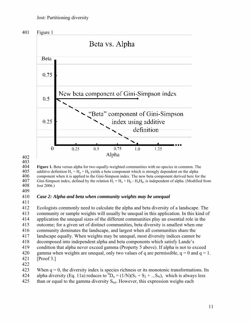
Figure 1. Beta versus alpha for two equally-weighted communities with no species in common. The additive definition Hγ = Hα + Hβ yields a beta component which is strongly dependent on the alpha component when it is applied to the Gini-Simpson index. The new beta component derived here for the Gini-Simpson index, defined by the relation Hγ = Hα + Hβ - HαHβ, is independent of alpha. (Modified from Jost 2006.) Case 2: Alpha and beta when community weights may be unequal Ecologists commonly need to calculate the alpha and beta diversity of a landscape. The community or sample weights will usually be unequal in this application. In this kind of application the unequal sizes of the different communities play an essential role in the outcome; for a given set of distinct communities, beta diversity is smallest when one community dominates the landscape, and largest when all communities share the landscape equally. When weights may be unequal, most diversity indices cannot be decomposed into independent alpha and beta components which satisfy Lande’s condition that alpha never exceed gamma (Property 5 above). If alpha is not to exceed gamma when weights are unequal, only two values of q are permissible, q = 0 and q = 1. [Proof 3.] When q = 0, the diversity index is species richness or its monotonic transformations. Its alpha diversity (Eq. 11a) reduces to 0Dα = (1/N)(S1 + S2 + ...SN), which is always less than or equal to the gamma diversity Stot. However, this expression weighs each

11


426 427 428 429 430 431 432 433 434 435 436 437 438 439 440 441 442 443 444 445 446 447 448 449 450 451 452 453 454 455 456 457 458 459 460 461 462 463 464 465 466 467 468 469 470

community equally regardless of its true weight, so it is not a satisfactory measure when community weights are important. When q = 1, the diversity index is Shannon entropy (or any monotonic transformation of it). This always satisfies Lande’s condition that alpha not exceed gamma, because it is a concave function (Lande 1996). Its numbers equivalent, the true alpha diversity, is given by Eq. 11b, the exponential of the traditional alpha Shannon entropy. Therefore, when weights may be unequal, Shannon measures (q = 1) are the only diversity measures that can be decomposed into independent alpha and beta components satisfying Properties 1-5 above. “One expects that deductions made from any other information measure, if carried far enough, will eventually lead to contradictions” (Jaynes 1957). 6. Traditional diversity indices are superfluous Jost (2006) showed that for diversity analyses of single communities, most traditional diversity indices are superfluous. Their numbers equivalents are the biologically meaningful entities, and these could be expressed more simply and directly in terms of q and the basic sums qλ, rather than calculating indices and then converting these to their numbers equivalents. This conclusion can now be extended to multiple-community diversity analyses when the communities have equal weights (the only case for which there is a choice of diversity measures other than Shannon measures). In fact the unifying mathematics works even when weights are unequal, but non-Shannon measures are prohibited in this case because alpha could exceed gamma. The new expression for true alpha diversity, Eq. 11 (the numbers equivalent of the properly-defined alpha component of a diversity index), is a function only of the species frequencies, the community weights, and the exponent q; for a given value of q it is independent of the diversity index used. The same applies to true gamma diversity (the numbers equivalent of the diversity index of the pooled samples), and since true beta diversity (the numbers equivalent of the beta component of a diversity index) equals true gamma diversity divided by true alpha diversity for all standard diversity indices, true beta diversity also depends only on the species frequencies, the community weights, and q. Diversity indices are therefore superfluous; for a given value of q, all standard diversity indices give the same final numbers equivalents. For example the Gini-Simpson index, the Simpson concentration, the inverse Simpson concentration, the Renyi entropy of degree 2, and the Hurlbert-Smith-Grassle index with m = 2 all give exactly the same true alpha, beta, and gamma diversities for any given set of communities. These indices can therefore be bypassed and the final numbers equivalents can be formulated more simply in terms of q and the sums qλ. For the purpose of calculating true alpha, beta, and gamma diversities (numbers equivalents), indices add nothing except unnecessary calculations. In the index-free description of diversity, with all community weights equal (the only case in which non-Shannon measures are valid), for q ≠ 1 the alpha sum qλα is the mean

12


of the individual community sums, (1/N) ∑=

N

1j

qλj. The gamma sum qλγ is calculated from

the pooled samples (as [((1/N)(p

471

472

473 474 475 476 477 478 479 480 481 482

483

484

485 486 487 488 489 490 491 492 493 494 495 496 497 498 499 500 501 502 503 504 505 506 507 508 509 510 511 512

∑=

S

1ii1 + pi2 + ...+ piN) q]). These are transformed into true

alpha, beta, and gamma diversities of order q (for q ≠ 1) using Eq. 2, and Whittaker’s law is used to find the true beta diversity: Alpha diversity of order q: qDα = qλα 1/(1-q) (16a-c) Gamma diversity of order q: qDγ = qλγ 1/(1-q)

Beta diversity of order q: qDβ = qDγ / qDα = (qλγ /qλα)1/(1-q) ≡ qλβ 1/(1-q). These are undefined when q =1, but their limits exist as q approaches 1, yielding the exponential of Shannon alpha, beta, and gamma entropies. The index-free description of diversity is therefore continuous in q. In fact the precursors to Eq. 16a-c are all mathematically valid even when weights are unequal, and their limits as q approaches unity give (see Eq. 11b): 1Dα = exp[-w1∑

=

S

1i

(pi1 ln pi1 ) + - w2∑=

S

1i

(pi2 ln pi2 ) + ...] (17a-c)

1Dγ = exp[∑ -(w=

S

1i1pi1 + w2pi2 + ...) ln(w1pi1 + w2pi2 + ...)]

1Dβ = 1Dγ / 1Dα It is remarkable that all of Shannon’s information functions come out of this theory automatically without reference to information theory. As shown earlier, these Shannon measures, Eqs.15a-c, are the only meaningful diversity measures (the only ones satisfying the properties of Section 2) when community weights are unequal. 7. Relation between the new beta diversity and indices of community similarity and overlap Beta diversity is inversely related to most concepts of community similarity. Suppose we are comparing the compositional similarity of a set of N communities. The sizes of the communities are irrelevant to this comparison and so their statistical weights are taken to be equal. If the equally weighted communities have a high compositional similarity, then the set of communities must have a low beta diversity. Conversely if the communities have low similarity, their beta diversity must be high. The relation can be made rigorous: if conclusions based on a similarity, overlap, or homogeneity measure are to be logically consistent with (not contradict) conclusions based on a given diversity measure, then the similarity measure must be a monotonic transformation of the diversity measure’s beta diversity. [Proof 4.] Different kinds of transformations of beta diversity will illuminate different aspects of its behavior. Each transformation generates an infinite family of similarity measures parameterized by q, which controls the sensitivity of the measures to rare or common species. The most popular similarity and overlap measures of ecology are in fact transformations of the new beta diversity qDβ. The true beta diversity of order 1, the numbers equivalent of beta Shannon entropy, can be transformed into MacArthur’s (1965) homogeneity measure:

13


M = = 1/ 1Dβ = exp(H α Shannon)/exp(H γ Shannon). (18) 513 514 515 516 517 518 519 520 521 522 523 524 525 526 527 528 529 530 531 532 533 534 535 536

537

538 539 540 541 542 543 544 545 546 547 548 549 550 551 552 553 554 555 556 557

It answers the question, "What proportion of total diversity is found within the average community or sample?" For N equally-weighted communities, it can be generalized to other values of q: M = 1/ qDβ (19) which ranges from 1/N (when all communities are completely distinct) to unity (when all communities are identical). The lower limit of this simple homogeneity measure depends on the number of samples or communities. It would be easier to interpret and more useful in comparisons if its lower limit were zero. For N equally weighted communities the measure qS = (1/qDβ - 1/ N)/ (1-1/N) (20) is the simplest linear transformation of 1/qDβ which has this property. It is zero when all N communities in the region are completely distinct from each other, and is unity when all N communities are identical in species composition. It is linear in the proportion of regional diversity contained in the average community. Jost (2006) shows that when this measure is applied to a pair of equally-weighted communities, it produces the Jaccard index when q = 0, and the Morisita-Horn index when q = 2. Equation 20 may be considered the generalization of these similarity measures to N communities and to arbitrary values of q. Shannon measures (and only Shannon measures) are valid not only when statistical weights are equal but also when they are unequal, and in that case MacArthur’s measure, Eq. 18, is still a valid measure of regional homogeneity. Its minimum value is

1/ exp[-∑ (w=

N

1jj ln wj )] ≡ 1/1Dw (21)

which is the reciprocal of the numbers equivalent of the Shannon entropy of the weights. It takes this value when all communities are completely distinct. Its maximum value is unity when all communities are identical. This homogeneity measure can therefore be converted into a relative index of homogeneity that goes from 0 (all communities distinct) to unity (all communities identical), like Eq. 20: Relative homogeneity = (1/1Dβ - 1/ 1Dw)/ (1-1/1Dw). (22) This measure, like Eq. 18, is useful in the interpretation of the results of additive partitioning using Shannon measures. A direct measure of pairwise community overlap is often the most easily interpreted similarity measure. For this purpose the weights of the two communities are irrelevant and are taken to be equal. The new beta diversity can be transformed into such a measure of overlap: Overlap (of order q) ≡ [(1/ qDβ) q-1

– (1/2)q-1] / [1– (1/2)q-1]. (23) Jost (2006) shows that when this measure is applied to a pair of equally weighted communities, it produces the Sørensen index when q = 0 and the Morisita-Horn index when q = 2. In the limit as q approaches unity it becomes Overlap of order 1 = (ln 2 - Hβ Shannon) / ln 2 (24) which is the Horn index of overlap, the only measure of overlap that does not disproportionately favor either rare or common species. For all values of q, Eq. 23 and 24

14


558 559 560 561 562 563 564 565 566 567 568 569 570 571 572 573 574 575 576 577 578 579 580 581 582 583 584 585 586 587 588 589 590 591 592 593 594 595 596 597 598 599 600 601 602 603

are true overlap measures in the sense of Wolda (1981): when applied to two communities each consisting of S equally common species, with C species shared between the communities, they give C/S, the proportion of a community’s species which are shared. Alternatively, for multiple equally-weighted communities, true beta diversity can be transformed into the turnover rate per sample (generalizing Harrison et al. 1992) by taking (qDβ-1)/(N-1). (25) where N is the number of samples. This ranges from zero (no turnover between samples) to unity (each sample is completely different from every other sample). All similarity measures based on the new beta diversity inherit its independence from alpha, a desirable property (Wolda 1981, Magurran 2004). A very large number of similarity indices are inconsistent with the beta diversity of any standard diversity index. These include the Bray-Curtis index (Bray and Curtis 1957), Canberra metric (Lance and Williams 1967), Renkonen index (Renkonen 1938), and many others. Conclusions based on such measures can contradict conclusions based on valid diversity indices, and their possible dependence on alpha make it difficult to disentangle mathematical artifacts from biologically meaningful effects. Traditional similarity measures have a strong negative bias when sample size is small; even two samples from the same population will often appear to be dissimilar according to these measures (Lande 1996). Expressing a similarity measure as a transformation of beta helps solve this problem, since beta is a simple function of alpha and gamma, and almost-unbiased estimators of alpha and gamma exist for many diversity measures (e.g. Chao and Shen 2003). 8. Examples Tundra and rainforest revisited The new measures give very different results than the traditional measures when applied to the examples of the Introduction. The traditional Gini-Simpson “beta” for the two intercontinental rainforest samples was 0.9861 - 0.9721 = 0.014, paradoxically lower than the “beta” diversity of the homogeneous antarctic tundra. This “beta” does not, by itself, tell the amount of turnover between samples, because of its dependence on alpha (Fig. 1). Depending on alpha, a “beta” value of 0.014 can mean that the samples are nearly identical, somewhat similar, or completely different. The similarity measure commonly used with the additive definition, Hα/Hγ or 1- (Hβ/Hγ) (Lande 1996), does not resolve this ambiguity. For the intercontinental rainforest data set, using the Gini-Simpson index, this “similarity” between samples is 0.99, even though the samples share no species. (The measure would have a value of 1.00 if both communities were identical in species composition and frequency.) This “similarity” between completely distinct intercontinental rainforests is even greater than the “similarity” between the

15


604 605 606 607 608 609 610 611 612 613 614 615 616 617 618 619 620 621 622 623 624 625 626 627 628 629 630 631 632 633 634 635 636 637 638 639 640 641 642 643 644 645 646 647 648 649

homogeneous tundra samples (0.95). The new Gini-Simpson beta component is, by Eq. 15d, (Hγ - Hα)/(1- Hα) = (0.9861 - 0.9721)/(1- 0.9721) = 0.50. This new beta has a different character than the tradition “beta”. Using this method (which is standard in most sciences; Aczel and Daroczy 1975, Tsallis and Brigatti 2004, Keylock 2005) a Gini-Simpson index of 0.5 has the same absolute and invariable interpretation whether it comes from the alpha, beta, or gamma component of the index. The interpretation is given by its numbers equivalent, which is (from Table 1) 1/(1-0.50) = 2.0. Thus a Gini-Simpson index of 0.50 is always, in any context, the amount of diversity produced by 2.0 equally-likely, completely distinct alternatives. In the context of this beta diversity calculation, it correctly indicates that there are two equally-weighted completely distinct intercontinental rainforest samples in the data set. The calculation of true beta diversity of the rainforest samples using Shannon entropy (the order 1 diversity measure) is similar to the calculation using the Gini-Simpson index. The beta component of the Shannon entropy is (by Eq. 15b) Hγ-Hα, which is 0.6931. A Shannon entropy of 0.6931 has the same interpretation no matter where it came from. As always, this interpretation is given by its numbers equivalent, which is (from Table 1) exp(0.6931) = 2.0. A Shannon entropy of 0.6931 is always the amount of diversity produced by 2.0 equally-likely, completely distinct alternatives. Here it indicates that there are two equally-weighted completely distinct intercontinental rainforest samples in the data set. The agreement with the Gini-Simpson result is not an accident; the numbers equivalent of the correctly-calculated beta component of any standard diversity index will be 2.0 for this data set, because the data set consists of two equally large completely distinct samples. In the new approach the antarctic tundra samples always have a lower beta diversity than the intercontinental rainforest samples, in contrast to the traditional approach which ranks them in reverse when using the Gini-Simpson index. The new beta component of the Gini-Simpson index for the antarctic samples is (0.4199-0.400)/(1-.400) = 0.03 and its numbers equivalent, the true beta diversity of order 2, is 1.03. By this measure there are effectively only 1.03 distinct communities in this data set, meaning that the two samples are almost identical. The beta Shannon entropy is 0.02 and its numbers equivalent, the true beta diversity of order 1, is exp(.02) = 1.02. By this measure also the samples are almost identical. The beta component of species richness is 1.0, which is its own numbers equivalent. By this measure the communities are truly identical (since they share all species and this measure ignores frequencies). As shown in Section 6, traditional diversity indices are superfluous and the true diversities of any order q can be calculated directly from the basic sums qλ (or, for q =1, from Eq. 17a-c). For example, instead of using the Gini-Simpson index to calculate alpha, beta, and gamma diversities of order 2, we can calculate them more simply as follows: 2λ1 (Panamanian rainforest sample) = 0.049171219 2λ2 (Malaysian rainforest sample) = 0.00656619

16


2λ α (average of the basic sums of the samples) = 0 .0278839 650 651 652 653 654 655 656 657 658 659 660 661 662 663 664 665 666 667 668 669 670 671 672 673 674 675 676 677 678 679 680 681 682 683 684 685 686 687 688 689 690 691 692 693 694 695

2λ γ (pooled samples) = 0.013941 The true beta diversity of order 2 is therefore (Eq.16c): (qλγ /qλα)1/(1-q) = (0.013941 / 0.0278839) 1/(1-2) = 2.000 in agreement with the Gini-Simpson result. For any data set, all order 2 diversity indices will always give the same true beta diversity (the numbers equivalent of its beta component) as this direct index-free calculation. In general the results will depend on the order q, but if the samples are completely distinct (as in this case), or if they are perfectly identical, the results will be the same for all q. The similarity measures given in Section 7 are helpful in interpreting the new beta diversity. For the intercontinental rainforest samples, for any standard diversity index the proportion of regional diversity contained in the average community (Eq. 19) is 1/2; the similarity measure Eq. 20 is zero, and the overlap between communities (Eq. 23) is also zero. The turnover rate per community (Eq. 25) is 1.00 for any index, indicating complete turnover between communities. These same measures clearly show that the antarctic communities are homogeneous. For the true diversity of order 2 the beta diversity equals 1.03, so the proportion of regional diversity contained in the average community (Eq. 19) is 0.97; the similarity measure Eq. 20 is 0.94, and the overlap between communities (Eq. 23) is also 0.94. The community turnover rate (Eq. 25) is 0.03, indicating that there is almost no turnover between these communities. Beta diversity of a landscape, and analysis of heirarchical diversity components In the previous example the statistical weights of the two communities in each data set were taken to be equal; this meant we could legitimately use the full range of diversity indices rather than just Shannon measures (Case 1 of Section 5). This is not the case when calculating the alpha, beta, and gamma diversities of a landscape, where population density is not uniform, resulting in unequal statistical weights for different samples or communities (Case 2 of Section 5). The proofs of Sections 4 and 5 show that under these circumstances only Shannon measures can be decomposed into meaningful independent alpha and beta components. The additive definition of beta is valid for Shannon entropy (Eq. 8b), so the standard techniques of additive partitioning can be used with this index (but only with this index) to study the heirarchical partitioning of diversity (within-samples, between samples within communities, between communities, etc). One modification is necessary; the final results need to be converted to their numbers equivalents, the exponentials of Shannon alpha, beta, and gamma entropies, before they can be properly interpreted. Thus Lande’s similarity or homogeneity measure Hα/Hγ must be replaced by MacArthur’s measure, exp(Hα)/exp(Hγ); otherwise the “similarity” value will be inflated as in the intercontinental rainforest example above. MacArthur’s measure correctly gives the proportion of regional diversity contained in the average sample. The relative homogeneity, Eq. 22, is also useful in analyzing the results. (Alternatively, the entire partitioning could have been done multiplicatively using the numbers equivalents from the beginning.The results are the same.)

17


696 697 698 699 700 701 702 703 704 705 706 707 708 709 710 711 712 713 714 715 716 717 718 719 720 721 722 723 724 725 726 727 728 729 730 731 732 733 734 735 736 737 738 739 740 741

9. Conclusions Limitations of additive partitioning of diversity Additive partitioning of diversity into heirarchical components (Lande 1996; see Veech et al. 2002 for a complete review of its history) is a popular method of diversity analysis, in which beta is compared between different heirarchical levels. However, the technique only makes sense if the beta it produces is independent of alpha; if beta depends on alpha, the beta values between different heirarchical levels cannot be compared with each other (since each level has a higher alpha than the preceding level) nor with the beta values of other ecosystems with different alpha values. The proofs of Sections 4 and 5 show that when community statistical weights differ the only index which can be additively partitioned into independent alpha and beta components is the Shannon entropy. The frequently recommended Gini-Simpson index cannot be used; its decomposition into independent alpha and beta components is only possible when the statistical weights of all samples are equal, and even then the decomposition is not additive. Also, for many diversity indices (including Shannon entropy and the Gini-Simpson index) the similarity measure used with additive partitioning, Hα/Hγ, necessarily approaches unity for high-diversity ecosystems, regardless of the amount of differentiation between samples. If the Gini-Simpson index is used as the diversity measure, it is mathematically impossible for the “similarity” to be lower than the alpha “diversity”. This happens because Hγ for this index is strictly less than unity; therefore the quotient Hα/Hγ must always be greater than Hα. Since Hα for this index often exceeds 0.95 in tropical ecosystems, a set of tropical samples will often have a Gini-Simpson “similarity” greater than 0.95 even if they have nothing in common (i.e. even when they are completely distinct in species composition and frequencies). This measure should not be used to draw conclusions about differences in composition between samples (contrary to the recommendations of Veech et al. 2002 and contrary to the practices of most of the studies cited therein). The importance of numbers equivalents Many biologists think of diversity indices simply as intermediate steps in the calculation of statistical significance. On this view, one measure of diversity is as good as another, as long as it can be used to calculate the statistical significance of the effect under study. A moment's reflection, however, shows that this is not reasonable. A very tiny bias in a coin can be detected at any desired significance level if enough trials are made, but it is still an insignificant bias in practice. The statistical significance of an effect has little to do with the actual magnitude or biological significance of the effect, which is the really important scientific question.We therefore need measures that behave intuitively so that we can judge changes in their magnitudes.

18


742 743 744 745 746 747 748 749 750 751 752 753 754 755 756 757 758 759 760 761 762 763 764 765 766 767 768 769 770 771 772 773 774 775 776 777 778 779 780 781 782 783 784 785 786

Ecologists’ intuitive theoretical concept of diversity corresponds not to the raw values of diversity indices but to their numbers equivalents (Hill 1973, Peet 1974, Jost 2006). Converting diversity indices to their numbers equivalents allows us to judge changes in their magnitude, because numbers equivalents posess the “doubling” property (Section 3) that characterizes our intuitive concept of diversity. When alpha, beta, and gamma are expressed as numbers equivalents, their magnitudes have simple intuitive interpretations in terms of the number of equally common species or the number of distinct equally large communities; it is easy to visualize these and easy to judge the importance of changes in their magnitudes. Numbers equivalents let us move beyond mere statistical conclusions. Numbers equivalents correct the anomalous behavior of the “similarity” measure Hα/Hγ described above; converting the raw alpha and gamma indices in this ratio to their numbers equivalents produces a similarity or homogeneity measure, qDα /qDγ, that accurately reflects the proportion of regional diversity contained in the average sample. This measure equals 1/N when applied to N equally-weighted, completely distinct samples, no matter which diversity index is used and no matter what the species frequencies, so it provides an absolute benchmark from which to judge the distinctness of a set of samples. Equation 20 transforms this onto the interval [0,1]. All standard diversity indices of a given order group communities into the same "level surfaces" and differ only in the way they label these level surfaces. It is therefore reasonable to standardize on the labelling system that gives the most intuitive results, the numbers equivalents; in doing so we are not ignoring the many other aspects of compositional complexity but rather converting them all to common and intuitive units. Numbers equivalents also provide a powerful mathematical tool for proving index-independent theorems of great generality. The most interesting of these theorems is the main result of this paper, a generalization of Whittaker’s law: if alpha and beta components of a diversity index are independent, their numbers equivalents must be multiplicative. That is, the product of their numbers equivalents must give the numbers equivalent of the gamma diversity index. Numbers equivalents reveal a deep unity between all standard diversity indices. The numbers equivalents of all of them are given by a single equation (Eq. 2). The numbers equivalents of standard diversity indices also generate and unify the standard similarity and overlap indices of ecology (Section 7). New alpha and beta versus old For most non-Shannon indices, the traditional additive beta component was not independent of the alpha component, and had no special value when all communities were distinct. The “numbers equivalent” of the beta component of an index bore no relation to the “numbers equivalents” of the alpha and gamma components of that index. The beta component often did not use the same metric as the alpha component, in the

19


787 788 789 790 791 792 793 794 795 796 797 798 799 800 801 802 803 804 805 806 807 808 809 810 811 812 813 814 815 816 817 818 819 820 821 822 823 824 825 826 827 828 829 830 831 832

sense that a given number denoted different amounts of diversity or uncertainty depending on which component it came from. These anomalies are corrected by the new alpha and beta components of diversity indices. For N equally-weighted communities (the only case for which non-Shannon indices are valid), the new alpha components of all non-Shannon standard diversity indices are given by Eq. 12 (the alpha Shannon entropy is the same as the traditional one); the new beta components of the most common diversity indices are given by Eq. 15a-g. These alpha and beta now use exactly the same metric as gamma, and beta provides complete information about the relative degree of community complementarity, without confounding this with alpha. Converting these new alpha and beta components of a diversity index to their numbers equivalents makes them easily interpretable. For N equally-weighted communities (the only case for which non-Shannon indices are valid), the numbers equivalent of Hβ for any standard diversity index has a uniform interpretation, indicating the effective number of distinct communities in the region, which ranges from 1 to N. When there are N distinct equally-weighted communities, this true beta diversity is always N, regardless of the index used and regardless of the species frequencies. Diversity is most easily analyzed by bypassing traditional diversity indices and calculating the alpha, beta, and gamma numbers equivalents directly, using Eqs. 16 and 17. The numbers equivalents deserve to be considered the true alpha, beta, and gamma diversities (of order q) of the system under study. The order q determines the emphasis on the dominant species (with q greater than 1 emphasizing dominant species). Importance of Shannon measures Shannon measures are the only standard diversity indices that can be decomposed into meaningful independent alpha and beta components when community weights are unequal. Shannon measures do not need to be borrowed from information theory; the exponential of Shannon entropy and related functions are derived here from the natural conditions on beta discussed in Section 2. An often-repeated criticism of Shannon measures is that they have no clear biological interpretation. Shannon entropy does in fact have an interpretation in terms of interspecific encounters (Patil and Taillie 1982), and both HShannon and exp(HShannon) can be related to characteristics of maximally-efficient species keys (Jost 2006) and to biologically reasonable notions of uncertainty (Shannon 1948) and average rarity (Patil and Taillie 1982). Some authors (e.g. Lande 1996, Magurran 2004) recommend the Gini-Simpson index over Shannon entropy on the grounds that the former converges more rapidly to its final value and has an unbiased estimator. However, the Gini-Simpson index and all other order 2 indices emphasize dominant species (which is why it converges more rapidly to its final value), and this may not always be desirable. Furthermore, since the Gini-

20


833 834 835 836 837 838 839 840 841 842 843 844 845 846 847 848 849 850 851 852 853 854 855 856 857 858 859 860 861 862 863 864 865 866 867 868 869 870 871 872 873 874 875 876 877

Simpson index cannot generally be decomposed into independent alpha and beta components which satisfy Lande’s condition that alpha never exceed gamma, it cannot be used for studies that involve landscape alpha or beta. (It --or rather its numbers equivalent-- is fine for studies comparing communities directly, using equal statistical weights, when it is desired to emphasize the dominant species.) The recent development of a nearly unbiased nonparametric estimator for Shannon entropy (Chao and Shen 2003) makes sampling criticisms less relevant. This nonparametric estimator for Shannon entropy converges rapidly with little bias even when applied to small samples. Some authors who are critical of Shannon measures because of their sampling properties (e.g. Magurran 2004) recommend species richness and its associated similarity and overlap measures, the Jaccard and Sorensen indices. These measures have worse sampling properties than Shannon measures (Lande 1996, Magurran 2004). Since they are completely insensitive to differences in species frequencies, they are poor choices for distinguishing communities or comparing pre- and post-treatment diversities, and they converge more slowly than any other measure as sample size increases. They are also not ecologically realistic; ecologically meaningful differences between communities are matters of differences in species frequencies, not in their mere presence or absence. Communities almost always have rare vagrants, but presence-absence measures give them the same weight as shared dominant species in calculating the similarity or overlap of two communities. Frequency data provide important information that should be used when available. The new expressions for alpha and beta remove the anomalies of the traditional definitions, and the conversion of properly-defined frequency-based measures to their numbers equivalents makes them linear with respect to our intuitive ideas of diversity. They are now almost as easy to interpret as species richness, and much more reliable and informative. The same is true for similarity and overlap measures; the Horn index of overlap (Eq. 24) is more informative, discriminating, and reliable than either the Jaccard or Sorensen indices. Species richness beta Much landscape data consists only of presence/absence records, which force us to use species richness as our diversity measure. The proofs of Section 5 show that species richness can only be partitioned into independent alpha and beta components if we treat each sample with equal statistical weight, and use Whittaker’s multiplicative formula. Only then will alpha, beta, and gamma satisfy the essential properties 1-5 described in Section 2. This beta diversity is not really a characteristic of the landscape but rather a direct measure of compositional similarity between N samples (without regard to their relative sizes). As such it is equivalent to the N-community generalization of the Sorensen or Jaccard indices, which are independent of alpha. The turnover rate (0Dβ-1)/(N-1) (Harrison et al.1992) is also independent of alpha and is a useful measure of regional heterogeneity. Scope of these results

21


The proof that Shannon measures are the only ones that can always be decomposed into meaningful independent alpha and beta components applies only to the class of standard diversity indices, as defined in Section 3. A few nonparametric diversity measures used in biology are excluded from this proof because they do not belong to this class. The Hurlbert-Smith-Grassle index for m > 2 is such a measure, since it cannot generally be written in terms of

878 879 880 881 882 883 884 885 886 887 888 889 890 891 892 893 894 895 896 897 898 899 900 901 902 903 904 905 906 907 908 909 910 911 912 913 914 915 916 917 918 919 920 921 922 923

qλ. Although nothing in the present paper excludes the possibility that this index may be decomposable into meaningful independent alpha and beta components when m is greater than 2, the index does fail to decompose when m = 2, and it seems unlikely that higher values of m would change this property. While Fisher’s alpha is not strictly a nonparametric index, it is sometimes used as if it were (Magurran 2004). The results presented here do not exclude the possibility that it could be decomposed into meaningful independent alpha and beta components for data from a log series distribution. However there are strong reasons to avoid this index for general use. When the data are not log-series distributed this index is difficult to interpret, and as it is usually calculated (Magurran 2004) it throws away almost all the information in the sample (since it depends only on the sample size and the number of species in the sample, not the actual species frequencies). For example, a sample containing ten species with abundances [91, 1, 1, 1, 1, 1, 1, 1, 1, 1] has the same diversity, according to this method of calculating Fisher’s alpha, as a sample containing ten species with abundances [10, 10, 10, 10, 10, 10, 10, 10, 10, 10], whereas ecologically and functionally the second community is much more diverse than the first. Relation of the new alpha and beta to results in other sciences Since 1988 physicists have begun to use new measures of entropy such as the HCDT or Tsallis entropy, which includes as special cases the standard diversity indices of biology: Shannon entropy, the Gini-Simpson index, and species richness minus one (Keylock 2005). Physicists have recently proposed a new definition of alpha or conditional HCDT entropy (Tsallis et al. 1998, Abe and Rajagopal 2001; in physics and information theory, the ecologists’ alpha is called the “conditional entropy”) which is identical to the expression that I have derived here (Eq. 10) from very different premises. They were led to this new definition of conditional or alpha entropy by thinking about theoretical issues in nonextensive thermodynamics, such as the thermodynamics of black holes and quantum-mechanical systems. Jizba and Arimitsu (2004) have proposed a definition of Renyi conditional entropy for thermodynamics, and this also turns out to be the same definition of alpha entropy that I have derived here. It is remarkable that studies of stars, electrons, and butterflies converge on these same expressions. 10. Acknowledgements I thank Anne Chao, Phil DeVries, Harold Greeney, Brad Jost, John Longino, Joseph Veech, Thomas Walla, and Don Waller for discussions on diversity measures, and

22


924 925 926 927 928 929 930 931 932 933 934 935 936 937 938 939 940 941 942 943 944 945 946 947 948 949 950 951 952 953 954 955 956 957 958 959 960 961 962 963 964 965 966 967 968

Nathan Mucchala for invaluable bibliographic help. This work was supported by grants from John and the late Ruth Moore to the Population Biology Foundation, by Steven Beckendorf and Cindy Hill, and by Nigel Simpson, O.B.E. 11. References Abe, S., and A. Rajagopal. 2001. Nonadditive conditional entropy and its significance for local realism. Physics Letters A 289: 157-164. Aczel, J., and Z. Daroczy. 1975. On Measures of Information and Their Characterization. – Academic Press, N.Y. Adelman, M. 1969. Comment on the H concentration measure as a numbers equivalent. The Review of Economics and Statistics 51: 99-101. Bray, J., and J. Curtis. 1957. An ordination of the upland forest communities in southern Wisconsin. Ecology Monographs 27: 325-349. Buzas, M., and L. Hayek. 1996. Biodiversity resolution: an integrated approach. Biodiversity Letters 3: 40-43. Chao, A., and T. Shen. 2003. Nonparametric estimation of Shannon’s index of diversity when there are unseen species in sample. Environmental and Ecological Statistics 10: 429-433. Condit, R., S. Hubbell, and R. Foster. 2005. Barro Colorado Forest Census Plot Data. URL http://ctfs.si/edu/datasets/bci. Gimaret-Carpentier, C., R. Pelissier, J.-P. Pascal, and F. Houllier. 1998. Sampling strategies for the assessment of tree species diversity. J. of Vegetation Science 9: 161-172. He, F. 2005. Hubbell’s fundamental biodiversity parameter and the Simpson diversity index. Ecolgy Letters 8: 386-390. Harrison, S., S. Ross, J. Lawton. 1992. Beta diversity on geographic gradients in Britain. J. Animal Ecology 61:151-158. Hill, M. 1973. Diversity and evenness: A unifying notation and its consequences. Ecology 54: 427-432. Jaynes, E. 1957. Information theory and statistical mechanics. Physical Review 106: 620-630.

23


969 970 971 972 973 974 975 976 977 978 979 980 981 982 983 984 985 986 987 988 989 990 991 992 993

994 995 996 997 998 999

1000 1001 1002 1003 1004 1005 1006 1007 1008 1009 1010 1011 1012 1013

Jizba, P. and T. Arimitsu. 2004. Generalized statistics: yet another generalization. Physica A 340: 110-116. Jost, L. 2006. Entropy and diversity. Oikos 113: 363-375. Keylock, C. 2005. Simpson diversity and the Shannon-Wiener index as special cases of a generalized entropy. Oikos 109: 203-207. Lance, G., and W. Williams. 1967. Mixed-data classificatory programs. 1. Agglomerative systems. Aust. Comput. J. 1: 15-20. Lande, R. 1996. Statistics and partitioning of species diversity, and similarity among multiple communities. Oikos 76: 5-13. Lewontin, R. 1972. The apportionment of human diversity. Evol. Biol. 6: 381-398. MacArthur, R. 1965. Patterns of Species Diversity. Biol. Rev. 40: 510-533. Magurran, A. 2004. Measuring biological diversity. Blackwell Publishing. Olszewski, T. 2004. A unified mathematical framework for the measurement of richness and evenness within and among communities. Oikos 104: 377-387. Patil, G. and C. Taillie. 1982. Diversity as a concept and its measurement. J. American Statistical Association 77: 548-561.

Peet, R. 1974. The measurement of species diversity. Annual Review of Ecology and Systematics 5: 285-307. Renkonen, O. 1938. Statistisch-ökologische untersuchungen über die terrestische käferwelt der finnischen Bruchmoore. Ann. Zool Soc Zool-Bot. Fenn Vanamo 6:1-231. Renyi, A. 1970. Probability theory. North-Holland Publishing Co. Shannon, C. 1948. A mathematical theory of communication. Bell System Technical Journal 27: 379-423, 623-656. Smith, W., and J. Grassle. 1977. Sampling properties of a family of diversity measures. Biometrics 33:283-292. Taneja, I. 1989. On generalized information measures and their applications. Advances in Electronics and Electron Physics 76: 327-413. Tsallis, C., and E. Brigatti. 2004. Nonextensive statistical mechanics: a brief introduction. Continuum Mech. Thermodynamics 16: 223-235.

24


1014 1015 1016 1017 1018 1019 1020 1021 1022 1023 1024 1025 1026 1027

Tsallis, C., R. Mendes., A. Plastino. 1998. The role of constraints within generalized nonextensive statistics. Physica A 261: 534–554. Veech, J., K. Summerville, T. Crist, and J. Gering. 2002. The additive partitioning of species diversity: recent revival of an old idea. Oikos 99: 3-9. Whittaker, R. 1972. Evolution and measurement of species diversity. Taxon 21: 213-251. Wilson, M., and A. Shmida. 1984. Measuring beta diversity with presence-absence data. Journal of Ecology 72: 1055-1064. Wolda, H. 1981. Similarity indices, sample size and diversity. Oecologia 50: 296-302.

25

in press, ecology, “concepts and synthesis” sectionloujost.com/statistics and physics/diversity...

Documents