In P. Husbands and I. Harvey, 1997, Proceedings of the Fourth European Conference on Artificial Life(Cambridge, MA: MIT Press, 1997), pp. 125-134.

A Comparison of Evolutionary Activity

in Arti�cial Evolving Systems and in the Biosphere

Mark A. Bedau, Emile Snyder, C. Titus Brown

Reed College, 3203 SE Woodstock Blvd., Portland, OR 97202, USA

Email: fmab, emile, browng@reed.edu

Norman H. Packard

Prediction Company, 236 Montezuma St., Santa Fe, NM 87501, USA

Email: n@predict.com

To appear in Phil Husbands and Inman Harvey, eds.,

Proceedings of the Fourth European Conference on Arti�cial Life, ECAL97,

MIT Press/Bradford Books, 1997.

Abstract

Bedau and Packard [7] devised an approach to

quantifying the adaptive phenomena in arti�cial

systems. We use this approach to de�ne two

statistics: cumulative evolutionary activity and

mean cumulative evolutionary activity. Then we

measure the dynamics of cumulative evolutionary

activity, mean cumulative evolutionary activity

and diversity, on an evolutionary time scale, in

two arti�cial systems and in the biosphere as re-

ected in the fossil record. We also measure these

statistics in selectively-neutral analogues of the

arti�cial models. Comparing these data prompts

us to draw three conclusions: (i) evolutionary

activity statistics do measure continual adaptive

success, (ii) evolutionary activity statistics can

be compared in arti�cial systems and in the bio-

sphere, and (iii) there is an arrow of increasing

cumulative evolutionary activity in the biosphere

but not in the arti�cial models of evolution. The

third conclusion is quantitative evidence that the

arti�cial evolving systems are qualitatively di�er-

ent from the biosphere.

1 Evolutionary Activity Trends

We propose a way to quantify certain long-term trends

involving adaptation in evolving systems, and we com-

pare such trends in the fossil record and in data from

two arti�cial evolving systems. Long-term patterns in

the history of life on Earth have been actively discussed

ever since evolution theory originated with Lamark and

Darwin. This is no surprise for those, like ourselves, who

agree with McKinney ([22], p. 28) that \[t]he concept

of `trend' is arguably the single most important in the

study of evolution."

This discussion of evolutionary trends has become con-

nected with myriad issues, including the role of adap-

tation in evolution, the directionality of evolution|

especially with respect to various kinds of complexity or

organization|and the allied general notion of progress.

Recent work on long-term trends in the history of life

on Earth spans the gamut from (i) studies of transi-

tions in the evolution that suggest directionality related

to taxonomic diversity [33], taxonomic survivorship [27],

or structural and functional complexity of organisms

[21]; to (ii) decrial of any suggestion of \progressive"

trends [12, 10, 13, 31], including those involving com-

plexity and adaptation; to (iii) an intermediate insistence

on \emphatic agnosticism" based on the di�culties of

quantifying and measuring complexity [25]. Controversy

about the adaptive signi�cance of long-term evolution-

ary trends partly re ects a broader controversy about

the role of adaptation in biotic evolution in general; work

on this topic spans another broad gamut, ranging from

a rejection of the notion that adaptation is quanti�able

or measurable [14] to experimental tests of adaptation

in evolving populations of bacteria [36]. And similar

themes are now surfacing in studies of arti�cial evolv-

ing systems, in which one �nds claims to have observed

long-term trends of \open-ended evolution" or \perpet-

ual novelty" [19, 29, 17].

Our concern in this paper is with trends involving

adaptation rather than complexity, and our primary aim

is to make a quantitative comparison of such trends in

model systems and in the biosphere. We think that adap-

tation is indeed quanti�able and measurable, using evo-

lutionary activity, an approach �rst introduced in the

context of model evolving systems [7] and here slightly

modi�ed so that it applies to both model evolving sys-

tems and to data from the fossil record. Our procedure

will be to compare the dynamics of evolutionary activ-

ity displayed in the fossil record with that displayed in

two arti�cial evolving systems|the Evita model and the

Bugs model. We hope our comparison of evolutionary

activity in arti�cial and natural systems will lead to a

better understanding of whether and, if so, why evolving

systems exhibit long-term trends involving adaptation.

Evolutionary activity (or \activity", as we will some-

times say for simplicity) is computed from data obtained

by observing an evolving system. In our view an evolv-

ing system consists of a population of components, all of

which participate in a cycle of birth, life and death, with

each component largely determined by inherited traits.

(We use this \component" terminology to maintain gen-

erality.) Birth, however, allows for the possibility of in-

novations being introduced into the population. If the

innovation is adaptive, it persists in the population with

a bene�cial e�ect on the survival potential of the compo-

nents that have it. It persists not only in the component

which �rst receives the innovation, but in all subsequent

components that inherit the innovation, i.e., in an en-

tire lineage. If the innovation is not adaptive, it either

disappears or persists passively.

The idea of evolutionary activity is to identify innova-

tions that make a di�erence. Generally we consider an

innovation to \make a di�erence" if it persists and con-

tinues to be used. Counters are attached to components

for bookkeeping purposes, to update each components'

current activity as the component persists and is used.

If the components are passed along during reproduction,

the corresponding counters are inherited with the com-

ponents, maintaining an increasing count for an entire

lineage. Two large issues immediately arise:

1. What should be counted as an innovation? In fact,

innovations may be identi�ed on many levels in most

evolving systems. We de�ne an innovation as the in-

troduction of a new component into the system. In

the case of Evita, the components are entire geno-

types. In the case of Bugs, they are also genotypes,

though in previous studies, innovations on the level

of individual alleles have been measured [7, 4]. For

the fossil record, components will be taxonomic fam-

ilies; an innovation is the appearance of a family in

the fossil record.

2. How should a given innovation contribute to the evo-

lutionary activity of the system? We measure ac-

tivity contributions by attaching a counter to each

component of the system. In all the work we present

here a component's activity counter is incremented

each time step if the component simply exists at that

time step. Though there are ways to re�ne this sim-

ple counting method, and we discuss some of them

below, we use this version because it is directly ap-

plicable to the fossil data.

More formally, let fi(t) indicate whether the ith com-

ponent is present in the record at time t:

fi(t) =

�1 if component i exists at t

0 otherwise: (1)

Then we de�ne the evolutionary activity ai(t) of the ith

component at time t as its presence integrated over the

time period from its origin up to t, provided it exists:

ai(t) =

� R t0fi(t)dt if component i exists at t

0 otherwise: (2)

Thus, ai is the ith component's activity counter. Note

that a di�erent resolution of the second issue above

would result in a di�erent formula for incrementing the

activity counters (as in reference [7]). The cumulative

evolutionary activity, A(t), at time t (which we will of-

ten call just \cumulative activity") is simply the sum of

the evolutionary activity of all components:

A(t) =Xi

ai(t): (3)

The diversity, D(t), is simply the number of components

present at t,

D(t) = #fi : ai(t) > 0g; (4)

where #f�g denotes set cardinality. Then, the mean cu-

mulative evolutionary activity, �A(t), (which we will often

call simply \mean activity") is the cumulative evolution-

ary activity A(t) divided by the diversity D(t):

�A(t) =A(t)

D(t): (5)

Note that the cumulative activity is the product of

a measure of diversity (the number of components D(t))

with a measure of duration or persistence (the mean evo-

lutionary activity �A(t)). These two aspects have already

been noted as characteristic of evolution [15]; we have

simply formed a measurable statistic with them.

A system could show signi�cant diversity increase over

time but not show signi�cant activity increase over time.

An example is an evolutionary system with a high mu-

tation rate. Diversity will be high compared to similar

systems with lower mutation rates, but activity will be

low compared to the same reference group.

The cumulative activity de�ned by equation 3 is only

one of a host of statistics that may be computed from

2

the activity counters faig de�ned in equation 2. In refer-

ence [7], for example, we argue for a di�erent statistic to

capture what we might intuitively identify with \adap-

tive evolutionary innovation". The cumulative activity

does not support such an interpretation; we use it here

for its computational ease and because we feel it broadly

re ects continual adaptive success in the evolutionary

processes we consider here.

As we have mentioned, evolutionary activity was �rst

developed and applied in the context of a model evolu-

tionary system [7]. The motivation for viewing evolution-

ary activity as a measure of adaptation during evolution

is particularly strong for such model systems, in large

part because of intuition obtained by the experimental

control they o�er. In particular, as we illustrate for the

Evita and Bugs models below, it is possible to \turn o�"

adaptation in a simulation, while leaving reproduction

and death, resulting in a random sampling of components

in the population, with no connection between the com-

ponents and the survivability of the components. This

sort of neutral analogue can then be compared with the

normal situation, in which speci�c properties of compo-

nents can have a very strong e�ect on their survivability.

The introduction of a new component that has a pos-

itive e�ect on survivability is strongly re ected in the

evolutionary activity.

The neutral analogue essentially produces a random

walk in the space of possible components, analogous to

other models of random evolution [28, 15]. Such mod-

els are relevant to biological evolution not necessarily

because they are plausible models in themselves but be-

cause they highlight those aspects of an evolving system,

if any, which are due to adaptation as against those which

are due merely to random processes and historical acci-

dent.

2 The Evita Model

The Evita model is a limited-interaction system consist-

ing of self-replicating strings of code, akin to Tierra [29]

and Avida [1]. As in Tierra and Avida, programs in

a customized assembly language replicate while subject

to \cosmic-ray" mutation. Unlike Tierra but like Avida,

these programs are limited in interaction to their nearest

neighbors on a two dimensional grid. And unlike both

Tierra and Avida, no code parasitism is allowed in Evita.

The di�erences between Tierra, Avida and Evita,

while not profound in outlook, are signi�cant. The 2-

D interaction ensures that the spread of information

throughout the population is dependent on the size of

the system; whereas Tierra allows instantaneous inter-

action between widely disparate areas, this cannot hap-

pen in Avida or Evita. Blocking parasitism and more

complicated interactions (e.g. hyperparasitism and code

pirating) allows us to study the root dynamics of these

systems.

The system is initialized with a single human-written

program placed randomly on an N by M grid. This

program then executes and reproduces; each o�spring is

placed within a small radius of the parent program on

the grid, and they then also start executing. When a

parent program can �nd no unoccupied grid locations

nearby, the system chooses randomly from the oldest of

its neighbors, \kills" that neighbor, and places the o�-

spring there. No other interaction between programs is

permitted.

During each \timestep" in this system the program at

each occupied grid spot receives a �xed amount of the

processor time. This time is allocated in a way that is

unbiased by position; hence, no organism can gain an ad-

vantage in its placement. In fact, the only real advantage

position can give is the relative �tness of the surrounding

population: it may be that the nearby creatures are less

�t, e.g. reproduce more slowly, than the creature placed

onto their edge.

Mutation rate is speci�ed in terms of the probabil-

ity per timestep that each given \codon" or assembly

language instruction in a genotype is mutated. Thus,

the probability that a given program su�ers a mutation

somewhere is proportional to its length; longer programs

are more likely to su�er a mutation. While the proba-

bility that a given program is mutated is independent of

the size of the population of programs, the probability

that a mutation occurs somewhere in the population is

clearly proportional to the population size. Typically,

mutation rates are speci�ed in terms of 10�5 mutations

per timestep: that is, a mutation rate of m would mean

that a given codon would mutate on average once ev-

ery 105

mtimesteps. This means, for example, that in a

run with 1600 creatures with an average length of 30

instructions, a mutation rate of 1 would cause one mu-

tation somewhere in the population approximately every

other timestep.

The model has a clear biological analogy. The sys-

tem represents a biological \soup", full of self-replicating

strands of code (similar to RNA). Survival is governed

primarily by reproductive speed, and evolution towards

faster programs is the behavior usually exhibited. This

kind of system, while extremely simple, shows interesting

evolutionary behavior. Many people have used Tierra,

Avida, and similar simple systems to examine a variety

of issues in evolutionary dynamics [29, 30, 1, 20, 35, 2].

Evita is explicitly designed so that the only way the

programs interact is through reproduction. On aver-

age, programs that reproduce faster will supplant their

more slowly reproducing neighbors. A program's rate

of reproduction or \gestation time" depends only on its

genotype, and a genotype's gestation time is the sole de-

terminant of the expected rate at which programs with

that genotype will produce o�spring. Thus, all signi�-

cant adaptive events in Evita are changes in gestation

3

time.

We also de�ne a neutral analogue of Evita, which dif-

fers from Evita only in that there is no chance that a

genotype's presence or concentration in the population

is due to its adaptive signi�cance. Nominal \programs"

exist at grid locations, reproduce and die. The neutral

model has two parameters: the number of mutations in

the population per timestep (possibly a vector), and the

number of \programs" that reproduce per timestep (pos-

sibly a vector). When the neutral model is due to have

a reproduction event, the self-reproducing \program" is

chosen at random from the population (with equal proba-

bility). When a \program" reproduces, its oldest neigh-

boring \program" dies and the new child occupies the

newly emptied grid location. Each \program" has a nom-

inal \genotype" which it's children inherit. Whenever a

mutation strikes a \program" it is assigned a new \geno-

type". The evolutionary dynamics in this neutral ana-

logue is reduced to a simple random walk in genotype

space [2]. Genotypes arise and go extinct, and their con-

centrations change over time, but the genotype dynamics

is only weakly linked to adaptation through the repro-

duction rate parameter determined by the normal model.

None of the dynamic of a genotype in the neutral ana-

logue is due to that genotype's adaptive signi�cance for

the genotypes have no adaptive signi�cance whatsoever.

By recording mutation rates and reproduction rates

from an actual Evita run, the neutral analogue can then

be run with these vectors as parameters. The behavior

of this neutral analogue allows us to determine which

aspects of the behavior of our original Evita run were

due to adaptation and which can be attributed to the

underlying non-adaptive architecture of the system.

3 The Bugs Model

The Bugs model consist of many agents that exist in a

spatial grid, sensing the resources in their local environ-

ment, moving as a function of what they sense, ingest-

ing the resources they �nd, and reproducing or dying

as a function of their internal resource levels. The Bugs

model is in a line of models that originated with Packard

[26] and has subsequently been evolving in various hands

[7, 8, 3, 5, 4, 6, 11]

The Bugs model's spatial structure is a grid of sites

with periodic boundary conditions, i.e., a toroidal lattice.

Besides the agents, all that exists in the world are 50 tiny

(3�3 sites) square blocks of resources, which are spread

over the lattice of sites and replenished as needed from

an external source. The resource distribution is static

in space and time because resources are immediately re-

plenished at a site whenever they are consumed. Never-

theless, since the agents constantly extract resources and

expend them by living and reproducing, the agents func-

tion as the system's resource sinks and the whole system

is dissipative.

Adaptation is resource driven since the agents need a

steady supply of resources in order to survive and re-

produce. Agents interact with the resource �eld at each

time step by ingesting all of the resources (if any) found

at their current location and storing it in their inter-

nal resource reservoir. Agents must continually replenish

this reservoir to survive for they must expend resources

at each time step to cover their (constant) \existence

taxes" and \movement taxes" (variable, proportional to

distance moved). If an agent's internal resource supply

drops to zero, it dies and disappears from the world.

Each agent moves each time step as dictated by its ge-

netically encoded sensorimotor map: a table of behavior

rules of the form if (environment j sensed) then (do

behavior k). Only one agent can reside at a given site

at a given time, so an agent randomly walks to the �rst

free site if its sensorimotor map sends it to a site which

is already occupied. An agent receives sensory informa-

tion about the resources (but not the other agents) in

the von Neumann neighborhood of �ve sites centered on

its present location in the lattice. An agent can discrim-

inate whether or not resources are present at each site

in its von Neumann neighborhood. Thus, each sensory

state j corresponds to one of the di�erent detectable local

environments (there are about 15 of these in the model

studied here). Each behavior k is either a jump vec-

tor between one and �fteen sites in any one of the eight

compass directions (north, northeast, east, etc.), or it is

a random walk to the �rst unoccupied site. This yields a

�nite behavioral repertoire consisting of (8�15)+1 = 121

di�erent possible behaviors. Thus, an agent's genotype,

i.e., its sensorimotor map, consist of a movement genet-

ically hardwired for each detectable environmental con-

dition. These genotypes are extremely simple, amount-

ing to nothing more than a lookup table of sensorimotor

rules. On the other hand, the space in which adaptation

occurs is vast, consisting of up to 12115 � 1032 distinct

possible genotypes.

An agent reproduces (asexually|without recombina-

tion) if its resource reservoir exceeds a certain threshold.

The parent produces one child, which starts life with half

of its parent's resource supply. The child also inherits its

parent's sensorimotor map, except that mutations may

replace the behaviors linked to some sensory states with

randomly chosen behaviors. The mutation rate parame-

ter determines the probability of a mutation at a single

locus, i.e., the probability that the behavior associated

with a given sensory state changes. At the extreme case

in which the mutation rate is set to one, a child's entire

sensorimotor map is chosen at random. The results pre-

sented here were all produced with the mutation rate set

to 0:05.

A time step in the simulation cycles through the en-

tire population and has each agent, in turn, complete the

following sequence of events: sense its present von Neu-

4

mann neighborhood, move to the new location dictated

by its sensorimotor map unless that site is already occu-

pied, in which case randomly walk to the �rst unoccupied

site, consume any resources found at its new location, ex-

pend enough resources to cover existence and movement

taxes, and then, if its resource reservoir is high enough

or empty, either reproduce or die.

Sensorimotor strategies evolve over generations. A

given simulation starts with randomly distributed agents

containing randomly chosen sensorimotor strategies.

The model contains no a priori �tness function, as

Packard (1989) has emphasized, so the population's size

and genetic constitution uctuates with the contingen-

cies of extracting resources. Agents with maladaptive

strategies tend to �nd few resources and thus to die,

taking their sensorimotor genes with them; by con-

trast, agents with adaptive strategies tend to �nd su�-

cient resources to reproduce, spreading their sensorimo-

tor strategies (with some mutations) through the popu-

lation.

In resource-driven and space-limited models like the

Bugs model observed population size is a good measure

of the �tness of the genotypes in the population. Sig-

ni�cant adaptive events typically create notable popula-

tion rises. Populations with behaviorally heterogeneous

strategies have a hard time surviving on the tiny 3�3blocks. Agents following di�erent behavioral strategies

will tend to collide, which will tend to bump one of them

o� the block into the resource desert. Thus, typically all

agents on a given 3�3 block follow exactly the same be-

havioral strategy. All the agents are in a holding pattern

continually cycling over a subset of the resource sites on

the tiny block. The strategies are typically simple be-

havioral cycles which jump through a short sequence of

sites on the block. The simplest cycles (period 2) con-

sist of jumping back and forth between two sites. The

next simplest strategy (period 3) cycles through a triple

of sites.

Behavioral strategies with higher periods have a se-

lective advantage (every thing else being equal). Since

a 3�3 block contains 9 distinct sites, it can support at

most a period 9 strategy. A period n strategy has room

for at most n agents. Thus, longer period strategies can

support larger populations because they can exploit more

of the available energetic resources. All agents on blocks

reproduce at the same rate, so a block with a larger pop-

ulation will produce o�spring at a higher rate. Thus,

blocks with populations with larger period strategies will

exert greater migration pressure and, thus, will enjoy a

selective advantage throughout the hundreds of tiny re-

source islands.

Thus, the main kind of adaptation that occurs in the

present Bugs model involves extending the period of an

existing strategy, which allows the population to exploit

more of the available resource sites. Thus, evolution in a

random �eld of 3�3 blocks tends to create populations

with higher period strategies.

As we did with Evita, we also create a neutral analogue

of the Bugs model, which di�ers from the Bugs only in

that a genotype's persistence is no re ection of its adap-

tive signi�cance. Nominal \agents" are born, live, repro-

duce, and die at rates determined exactly by the values of

those variables measured in a particular run of the nor-

mal Bugs model. (For this reason, the population time

series in �g. 3 for the normal Bug model and the neutral

analogue are exactly the same.) The distinctive feature

of the neutral analogue is that birth, reproduction and

death events happen to \agents" chosen at random from

among those present in the population. Each \agent"

has a nominal \genotype" which it inherited from its

parent unless it su�ered a mutation at birth (mutation

rate is another model parameter). The evolutionary dy-

namics of the neutral analogue of the Bugs model is a

random walk in genotype space. As with Evita's neutral

analogue, none of the dynamic of a given genotypes in

this neutral analogue of the Bugs model is due to that

genotype's adaptive signi�cance for it has no adaptive

signi�cance.

4 The Fossil Data

The fossil data sets indicate the geological stages or

epochs with the �rst and last appearance of taxonomic

families. The Benton data [9] covers all families in all

kingdoms found in the fossil record, for a total of 7111

families. The Sepkoski data [32] indicates the fossil

record for 3358 marine animal families. The duration

of di�erent stages and epochs varies widely, ranging over

three orders of magnitude. In order to assign a uniform

time scale to the fossil data, we converted stages and

epochs into time indications expressed in units of mil-

lions of years ago using Harland's time scale [16].

We are most interested in analyzing long-term trends

among fossil species, but we study fossil families because

much more complete data is available at this level of

analysis [37, 34]. Although fossil family data is certainly

no precise predictor of fossil species data, there is ev-

idence that species-level trends in the fossil record are

re ected at the family level (see [37] and the references

cited therein). Sepkoski and Hulver ([34], p. 14) summa-

rize the situation thus: \Although families do not display

all of the detail of the fossil record, they should be su�-

ciently sensitive to show major evolutionary trends and

patterns with characteristic timescales of �ves to tens of

millions of years". The trends we discuss in this paper

occur on time scales at least that long.

5 Results

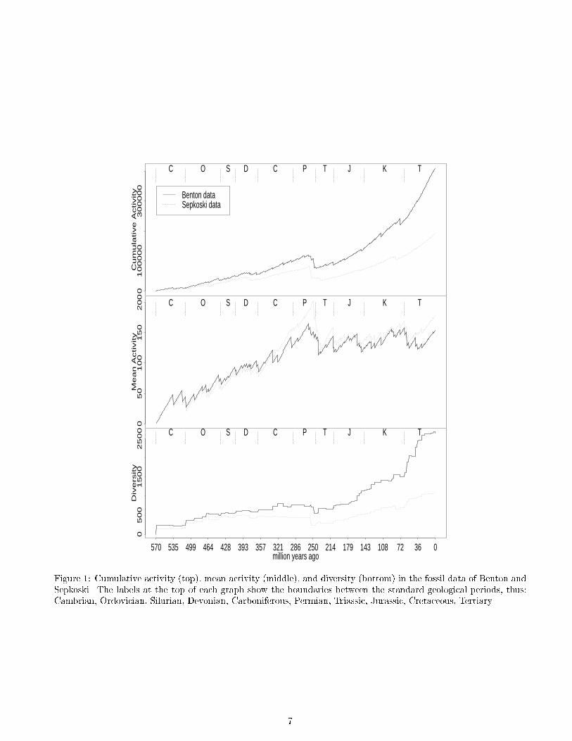
We computed the cumulative activity A(t), mean activ-

ity �A(t), and diversity D(t) in both the Benton and Sep-

5

koski fossil data sets (�g. 1). We also computed these

statistics from data produced by numerous simulations

of the Evita and Bugs models and chose representative

examples of the behavior of the statistics in Evita (�g. 2,

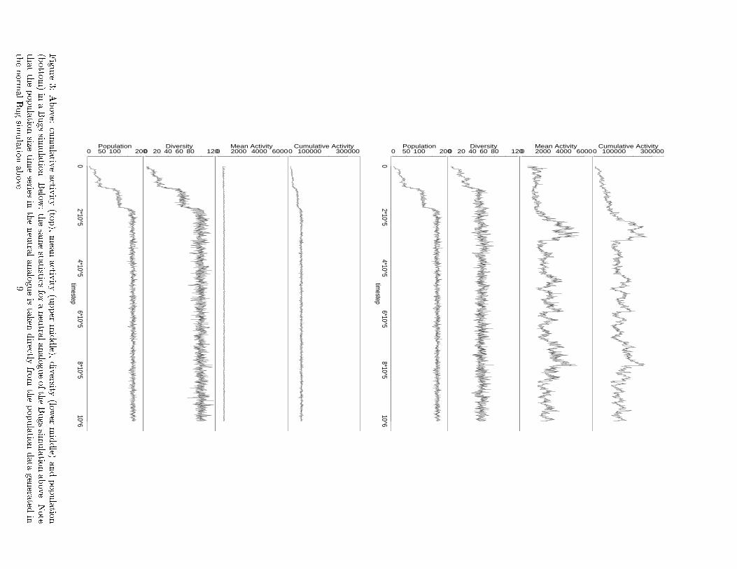
above) and Bugs (�g. 3, above). Finally, we computed

the same statistics from data produced by the neutral

analogue of Evita (�g. 2, below) and the neutral ana-

logue of the Bugs (�g. 3, below). In each case, the neu-

tral analogues were given parameters that exactly cor-

responded to those that governed the normal Evita and

Bugs runs.

We start the fossil data at the Cambrian explosion, due

to the relative crudeness of the preceding data. Visible

in the data are the major extinction events, such as the

largest one of all which ends the Permian period, and the

famous \K/T" extinction which involved the �nal demise

of the dinosaurs and is thought to have been caused by

a meteorite impact.

The Evita simulation shows the single ancestral pro-

gram quickly replicating enough to �ll up the 40�40grid. Most of the signi�cant improvements in reproduc-

tion rate occur at the very beginning of the simulation.

The local peaks in cumulative and mean activity dur-

ing the course of the simulation correspond to the in-

troduction of new genotypes that are neutral variants,

that is, they have the same adaptive signi�cance as the

other major genotypes in the population. In other words,

the bulk of this simulation consists of a random drift

among genotypes that are selectively neutral, along the

lines of the neutral theory of evolution [18]. Note that

these selectively-neutral variants are highly adaptive|

they are remarkably e�ective at the task of survival and

reproduction|but they just do this job equally well.

The �rst �fth of the Bugs simulation shows the popu-

lation adapting to the tiny blocks by increasing the cycle

size of their behavioral strategy. At least three major

innovations are recognizable in the population size dy-

namics. After the third major innovation, the evolution-

ary dynamics settles down into a random drift among

selectively-neutral variant genotypes, as in the Evita sim-

ulation.

Notice that there is a striking di�erence in the behav-

ior of the arti�cial models and their neutral analogues.

The neutral analogues do not produce anything like the

same statistics as the normal models (except for the pop-

ulation size in the Bug neutral analogue, of course, and

its shadow in the diversity and cumulative activity time

series). In particular, the cumulative and mean activity

values in the neutral analogues are negligible, by compar-

ison, while their diversity values are signi�cantly higher.

Evidently, adaptation has a dramatic e�ect when it is

allowed to a�ect the persistence of genotypes.

When we compare the evolutionary activity in these

three �gures, we see another striking di�erence. The fos-

sil data shows a long-term trend of cumulative activity

and diversity increasing more than linearly; fossil mean

activity increases roughly linearly into the Permian pe-

riod but then shows no further trend. But there is no

long-term trend in any statistic in the Evita and Bugs

data.

6 Discussion

We draw three main conclusions from our comparison

of evolutionary activity in arti�cial systems and in the

biosphere:

Conclusion 1: Cumulative evolutionary activity mea-

sures continual adaptive success for the evolutionary pro-

cesses we consider. This is clear for the two model sys-

tems primarily from the comparison provided by the neu-

tral analogues.

Conclusion 2: Cumulative evolutionary activity, along

with mean activity and diversity, are statistics that en-

able arti�cial evolutionary models to be compared quan-

titatively with evolution in the biosphere. It is clearly

possible to measure these statistics in arti�cial and nat-

ural systems. The proof of this pudding (conclusion 2)

comes in the eating.

Conclusion 3: If we accept conclusions 1 and 2, then

comparison of evolutionary activity in the data from

the fossil record and from the arti�cial evolving systems

reveals that long-term trends involving adaptation are

present in the biosphere but missing in the arti�cial mod-

els.

Our statistics show that the Evita and Bugs models do

not show comparable evolutionary activity to the evolu-

tionary activity of the biosphere indicated in the fossil

record. The primary di�erence is that cumulative evo-

lutionary activity and diversity of the biosphere shows

a strong increase on an evolutionary time scale, but the

Evita and Bugs models do not. Furthermore, the trends

shown in the biosphere are unlikely to be \accidental"

products of anything like the arti�cial models, for to our

knowledge the arti�cial models never exhibit such trends.

These strong increasing trends imply a directionality in

biological evolution that is missing in the arti�cial evo-

lutionary systems. Speci�cally, the biosphere shows an

arrow of increasing cumulative activity as well as an ar-

row of increasing diversity. These are directly related

since the post-Permian increase in cumulative activity is

driven mainly by the increase in diversity. (Recall that

cumulative activity is the product of diversity and mean

activity.) But the arrow of cumulative activity is espe-

cially interesting because of its implications about the

directionality of adaptation in biological evolution.

We view conclusion 3 as quantitative evidence that the

arti�cial models are qualitatively di�erent from the bio-

sphere. We suspect that no existing arti�cial system is

qualitatively like the biosphere. If this is right, then an

objective of the �rst importance is to devise an arti�-

cial model that captures the qualitative behavior of the

6

Cu

mu

lative

Activity

01

00

00

03

00

00

0

TKJTPCDSOC

Benton dataSepkoski data

Me

an

Activity

05

01

00

15

02

00

TKJTPCDSOC

million years ago

Div

ers

ity

570 535 499 464 428 393 357 321 286 250 214 179 143 108 72 36 0

05

00

15

00

25

00 TKJTPCDSOC

Figure 1: Cumulative activity (top), mean activity (middle), and diversity (bottom) in the fossil data of Benton and

Sepkoski. The labels at the top of each graph show the boundaries between the standard geological periods, thus:

Cambrian, Ordovician, Silurian, Devonian, Carboniferous, Permian, Triassic, Jurassic, Cretaceous, Tertiary.

7

Cumulative Activity0 20000 60000

Mean Activity0 50 100 150

timestep

Diversity

05*10^4

10^51.5*10^5

2*10^52.5*10^5

0 50 100 150 200Cumulative Activity

0 20000 60000Mean Activity

0 50 100 150

timestep

Diversity

05*10^4

10^51.5*10^5

2*10^5

0 50 100 150 200

Figure

2:Above:

cumulativ

eactiv

ity(to

p),meanactiv

ity(m

iddle),

anddiversity

(botto

m)in

anEvita

simulatio

n.

Belo

w:thesamesta

tisticsforaneutra

lanalogueoftheEvita

simulatio

nabove.

8

Cumulative Activity0 100000 300000

Mean Activity0 2000 4000 6000

Diversity0 20 40 60 80 120

timestep

Population

02*10^5

4*10^56*10^5

8*10^510^6

0 50 100 200Cumulative Activity

0 100000 300000Mean Activity

0 2000 4000 6000Diversity

0 20 40 60 80 120

timestep

Population

02*10^5

4*10^56*10^5

8*10^510^6

0 50 100 200

Figure

3:Above:

cumulativ

eactiv

ity(to

p),meanactiv

ity(upper

middle),

diversity

(lower

middle)

andpopulatio

n

(botto

m)in

aBugssim

ulatio

n.Belo

w:thesamesta

tisticsforaneutra

lanalogueoftheBugssim

ulatio

nabove.

Note

thatthepopulatio

nsize

timeseries

intheneutra

lanalogueistaken

directly

from

thepopulatio

ndata

genera

tedin

thenorm

alBugsim

ulatio

nabove.

9

biosphere.

We should note that the Evita and Bugs models dis-

allow any interesting interactions between organisms; no

predator-prey connections, no cooperation, no commu-

nication, nothing. But other arti�cial evolving models

do permit such interactions; e.g., Echo [17] and Tierra

[29]. We purposely focused this �rst study on especially

simple and well understood arti�cial models, to make it

easier to understand our results. An obvious next step is

to extend this study to more complex arti�cial models,

and this is part of current work. However, we conjecture

that the conclusions of this pilot study will hold for Echo

and Tierra as well.

The spatial and temporal scales of the Evita and Bugs

models are vastly smaller than the spatial and temporal

scale of the biosphere; and the same applies to the gen-

eral complexity of the systems. So perhaps these mod-

els should not be expected to show evolutionary activity

comparable to the biosphere. But we are con�dent that

scaling up space and time in the Evita and Bugs models

will not change the qualitative character of their activity

curves. This con�dence comes in part from observations

besides those reported here, but the conjecture is subject

to further direct empirical test. We similarly doubt that

simply making the models more \complex" will make the

quality of their behavior like that of the biosphere. We

think that the primary reason behind the biosphere's ar-

row of cumulative activity is that the dynamics of the

biosphere constantly create new niches and new evolu-

tionary possibilities through interactions between diverse

organisms. This aspect of biological evolution dramati-

cally ampli�es both diversity and evolutionary activity,

and it is an aspect not evident in these models.

The cumulative activity curve from the fossils is qual-

itatively similar to the initial transient of the Bugs cu-

mulative activity curve. So, the explanation of the qual-

itative di�erence in the long-term cumulative activity

shown in the fossils and in the arti�cial models might be

that the biosphere has been on some kind of \transient"

during the period re ected in the fossil record. The even-

tual statistical stabilization of the arti�cial evolving sys-

tems might be caused by the systems hitting their re-

source \ceilings"; in this case, growth in activity would

be limited by the �nite spatial and energetic resources

available to support adaptive innovations.

Evolution in the biosphere seems to have been free

from any inexorable resource ceilings, but we suspect

that this is largely because the biosphere's evolution con-

tinues to make new resources available when it creates

new niches. In fact, organisms occupying new niches

seem to create the possibility for yet newer niches; i.e.,

the space of innovations available to evolution is con-

stantly growing. We believe that this aspect of biological

evolution is the most important aspect missing from arti-

�cial models; simply increasing resources to the arti�cial

models studied here does not seem to signi�cantly a�ect

observed patterns of evolution. This suggests it would

be interesting to make a more careful comparison of the

fossil record data with initial transients of arti�cial sys-

tems, before the systems have exhausted the possibilities

for signi�cant adaptation. This will be a topic of future

work.

There are problems and pitfalls inherent in using the

fossil record to study long-term trends [27]. In particular,

the \pull of the present" is a well-known sampling bias

due to the fact that there are simply more recent fossils

to study than older fossils. Future work will investigate

the extent to which our analysis of fossil record trends

can be supported more rigorously.

We have tried to illustrate the value of studying evo-

lutionary trends by devising statistics that apply both

to data from the fossil record and to data generated by

arti�cial systems. Such statistics provide a normal form

for expressing conclusions about the behavior of arti�-

cial models and about how those models are relevant to

understanding biological evolution. Our work here has

focussed on the cumulative evolutionary activity statis-

tic, but this is not the only interesting statistic. As we

mentioned in section 1 above, other statistics de�ned in

terms of evolutionary activity highlight other kinds of

comparisons among systems, which might provide addi-

tional kinds of insights into evolutionary trends. Perhaps

yet further statistics unconnected with evolutionary ac-

tivity might �nd a similar use.

Comparing cumulative evolutionary activity in arti�-

cial systems and in the biosphere has lead to a negative

result (Conclusion 3): present arti�cial models of evo-

lution apparently lack some important characteristic of

the biosphere|whatever it is that is responsible for its

arrow of increasing cumulative activity. However, this

conclusion crystalizes an important constructive and cre-

ative challenge: to devise an arti�cial model of evolution

that succeeds where the present models fail. Here, again,

statistics like evolutionary activity show their value, for

they provide a quantitative test for whether an arti�cial

evolutionary model and a natural evolving system like

the biosphere exhibit the same kind of long-term trends

in adaptation.

Acknowledgements. Thanks to M. J. Benton and J.

J. Sepkoski, Jr., for making their fossil data available.

For helpful discussion, thanks to Bob French, Tim Keitt,

Dan McShea, Richard Smith, Peter Todd, the anony-

mous ECAL97 reviewers, the audience at the Santa Fe

Institute when MAB discussed some of these results in

July 1996, and the audience at the Cascade Systems

Society meeting when MAB presented this material in

March 1997.

10

References

[1] Adami, C., Brown, C. T. 1994. Evolutionary learn-

ing in the 2D arti�cial life system \avida". In R.

Brooks and P. Maes, (Eds.), Arti�cial Life IV (pp.

377-381). Cambridge, MA: Bradford/MIT Press.

[2] Adami, C., Brown, C.T., Haggerty, M.R.

1995. Abundance-distributions in arti�cial life and

stochastic models: \age and area" revisited. In F.

Mor�an, A. Moreno, J.J. Merelo, P. Chac�on, (Eds.),

Advances in Arti�cial Life (pp. 503{514). Berlin:

Springer.

[3] Bedau, M. A. 1994. The evolution of sensorimo-

tor functionality. In P. Gaussier and J. D. Nicoud

(Eds.), From Perception to Action (pp. 134{145).

New York: IEEE Press.

[4] Bedau, M. A. 1995. Three illustrations of arti�cial

life's working hypothesis. In W. Banzhaf and F.

Eeckman (Eds.), Evolution and Biocomputation|

Computational Models of Evolution (pp. 53{68).

Berlin: Springer.

[5] Bedau, M. A., Bahm, A. 1994. Bifurcation structure

in diversity dynamics. In R. Brooks and P. Maes,

(Eds.), Arti�cial Life IV (pp. 258{268). Cambridge,

MA: Bradford/MIT Press.

[6] Bedau, M. A., Giger, M., Zwick, M. 1995. Adaptive

diversity dynamics in static resource models. Ad-

vances in Systems Science and Applications 1, 1{6.

[7] Bedau, M. A., Packard, N. H. 1992. Measurement

of evolutionary activity, teleology, and life. In C. G.

Langton, C. E. Taylor, J. D. Farmer, S. Rasmussen,

(Eds.), Arti�cial Life II (pp. 431{461). Redwood

City, Calif.: Addison-Wesley.

[8] Bedau, M. A., Ronneburg, F., Zwick, M. 1992. Dy-

namics of diversity in an evolving population. In R.

M�anner and B. Manderick, (Eds.), Parallel Problem

Solving from Nature, 2 (pp. 94{104). Amsterdam:

North-Holland.

[9] Benton, M. J., ed. 1993. The Fossil Record 2. Lon-

don: Chapman and Hall.

[10] Dawkins, R. 1992. Progress. In W. F. Keller and

E. Lloyd, (Eds.), Keywords in Evolutionary Biology

(pp. 263{272). Cambridge, MA: Harvard University

Press.

[11] Fletcher, J., Zwick, M., Bedau, M. A. 1996. Depen-

dence of adaptability on environmental structure in

a simple evolutionary model. Adaptive Behavior 4,

283-315.

[12] Gould, S. J. 1989. Wonderful Life: The Burgess

Shale and the Nature of History. New York: Norton.

[13] Gould, S. J. 1996. Full House, New York: Harmony

Books.

[14] Gould, S. J., Lewontin, R.C. 1979. The spandrels of

San Marco and the Panglossian paradigm: a critique

of the adaptationist programme. Proceedings of the

Royal Society of London Series B 205, 581{598.

[15] Gould, S. J., Raup, D. M., Sepkoski, Jr., J. J. 1977.

The shape of evolution: a comparison of real and

random clades. Paleobiology 3, 23{40.

[16] Harland, W. B., Armstrong, R. L., Cox, A. V.,

Craig, L. E., Smith, A. G., Smith, D. G., 1990. A

Geological Time Scale 1989. Cambridge: Cambridge

University Press.

[17] Holland, J. H. 1992.Adaptation in Natural and Arti-

�cial Systems: An introductory analysis with appli-

cations to biology, control, and arti�cial intelligence,

2nd edition. Cambridge: MIT Press/Bradford

Books.

[18] Kimura, M. 1983. The Neutral Theory of Molec-

ular Evolution. Cambridge: Cambridge University

Press.

[19] Lindgren, L. 1992. Evolutionary phenomena in sim-

ple dynamics. In C. G. Langton, C. E. Taylor, J. D.

Farmer, S. Rasmussen, (Eds.), Arti�cial Life II (pp.

295{312). Redwood City, Calif.: Addison-Wesley.

[20] Maley, C. C. 1994. The computational completeness

of Ray's Tierran assembly language. In C. G. Lang-

ton, (Ed.), Arti�cial Life III (pp. 503{514). Red-

wood City, Calif.: Addison-Wesley.

[21] Maynard Smith, J., Szathmary, E. 1995. The Major

Transitions in Evolution. Oxford: Freeman.

[22] McKinney, M. L. Classifying and analysing evolu-

tionary trends. In K. J. McNamara, (Ed.), Evolu-

tionary Trends (pp. 28{58). Tucson: The University

of Arizona Press.

[23] McNamara, K. J. 1990. Preface. In K. J. McNamara,

(Ed.), Evolutionary Trends (pp. xv{xviii). Tucson:

The University of Arizona Press.

[24] McNamara, K. J., ed. 1990. Evolutionary Trends.

Tucson: The University of Arizona Press.

[25] McShea, D. W. 1996. Metazoan complexity and evo-

lution: is there a trend? Evolution 50, 477{492.

[26] Packard, N. H. 1989. Intrinsic adaptation in a sim-

ple model for evolution. In C. G. Langton, (Ed.),

Arti�cial Life (pp. 141{155). Redwood City, Calif.:

Addison-Wesley.

11

[27] Raup, D. M. 1988. Testing the fossil record for evo-

lutionary progress. In M. H. Nitecki, (Ed.), Evo-

lutionary Progress. Chicago: The University of

Chicago Press.

[28] Raup, D. M., Gould, S. J. 1974. Stochastic simula-

tion and evolution of morphology|towards a nomo-

thetic paleontology. Systematic Zoology 23, 305{

322.

[29] Ray, T. S. 1992. An approach to the synthesis of life.

In C. G. Langton, C. E. Taylor, J. D. Farmer, S.

Rasmussen, (Eds.), Arti�cial Life II (pp. 371{408).

Redwood City, Calif.: Addison-Wesley.

[30] Ray, T. S. 1993/1994. An evolutionary approach to

synthetic biology: zen and the art of creating life.

Arti�cial Life 1, 179{209.

[31] Ruse, M. 1996. Monad to Man: The Concept of

Progress in Evolutionary Biology. Cambridge, MA:

Harvard University Press.

[32] Sepkoski, Jr., J.J. 1992. A Compendium of Fossil

Marine Animal Families, 2nd ed. Milwaukee Public

Museum Contributions in Biology and Geology, Vol.

61.

[33] Sepkoski, J. J., Bambach, R. K., Raup, D. M.,

Valentine, J. W. 1981. Phanerozoic marine diversity

and the fossil record. Nature 293, 435{437.

[34] Sepkoski, J. J., Hulver, M. L. 1985. An atlas

of phanerozoic clade diversity diagrams. In J. W.

Valentine, (Ed.), Phanerozoic Diversity Patterns:

Pro�les in Macroevolution (pp. 11{39). Princeton:

Princeton University Press.

[35] Thearling, K., Ray, T. 1994. Evolving multi-cellular

arti�cial life. In R. Brooks and P. Maes, (Eds.), Arti-

�cial Life IV (pp. 283{288). Cambridge, MA: Brad-

ford/MIT Press.

[36] Travisano, M., J.A. Mongold, A.F. Bennet, R.E.

Lenski. 1995. Experimental tests of the roles of

adaptation, chance, and history in evolution. Sci-

ence 267, 87{90.

[37] Valentine, J. W. 1985. Diversity as data. In J. W.

Valentine, (Ed.), Phanerozoic Diversity Patterns:

Pro�les in Macroevolution (pp. 3{8). Princeton:

Princeton University Press.

12