in-kind transfers in brazil: household consumption and welfare … · 2016-09-05 · ficha...
TRANSCRIPT

UNIVERSIDADE DE SAtildeO PAULO
FACULDADE DE ECONOMIA ADMINISTRACcedilAtildeO E CONTABILIDADE
DEPARTAMENTO DE ECONOMIA
PROGRAMA DE POacuteS-GRADUACcedilAtildeO EM ECONOMIA
In-kind transfers in Brazil household
consumption and welfare effectsTransferecircncias em produto no Brasil efeitos sobre bem-estar e
consumo das famiacutelias
Bruno Toni Palialol
Orientadora Profa Dra Paula Carvalho Pereda
Satildeo Paulo - Brasil2016
Prof Dr Marco Antonio Zago
Reitor da Universidade de Satildeo Paulo
Prof Dr Adalberto Ameacuterico Fischmann
Diretor da Faculdade de Economia Administraccedilatildeo e Contabilidade
Prof Dr Heacutelio Nogueira da Cruz
Chefe do Departamento de Economia
Prof Dr Maacutercio Issao Nakane
Coordenador do Programa de Poacutes-Graduaccedilatildeo em Economia
BRUNO TONI PALIALOL
In-kind transfers in Brazil household
consumption and welfare effectsTransferecircncias em produto no Brasil efeitos sobre bem-estar e
consumo das famiacutelias
Dissertaccedilatildeo apresentada ao Programa dePoacutes-Graduaccedilatildeo em Economia do Depar-tamento de Economia da Faculdade deEconomia Administraccedilatildeo e Contabilidadeda Universidade de Satildeo Paulo como requisitoparcial para a obtenccedilatildeo do tiacutetulo de Mestreem Ciecircncias
Orientadora Profa Dra Paula Carvalho Pereda
Versatildeo Corrigida(versatildeo original disponiacutevel na Biblioteca da Faculdade de Economia Administraccedilatildeo e Contabilidade)
Satildeo Paulo - Brasil
2016
FICHA CATALOGRAacuteFICA
Elaborada pela Seccedilatildeo de Processamento Teacutecnico do SBDFEAUSP
Palialol Bruno Toni In-kind transfers in Brazil household consumption and welfare effects Bruno Toni Palialol -- Satildeo Paulo 2016 73 p Dissertaccedilatildeo (Mestrado) ndash Universidade de Satildeo Paulo 2016 Orientador Paula Carvalho Pereda
1 Economia de mercado 2 Medidas econocircmicas 3 Econometria
I Universidade de Satildeo Paulo Faculdade de Economia Administraccedilatildeo e Contabilidade II Tiacutetulo CDD ndash 3326323
Dedicada agravequeles com coragem de enfrentar
os desafios que a vida lhes impotildee
AgradecimentosEm primeiro lugar agradeccedilo agrave minha orientadora Paula Pereda pelo entusiasmo
inabalaacutevel e busca incessante por aprimoramentos Sem ela o presente trabalho certamente
natildeo teria sido possiacutevel
Agradeccedilo agrave minha matildee Sonia Toni pela paciecircncia compreensatildeo carinho e por
tornar os uacutetimos anos de trabalho um pouco mais confortaacuteveis
Agrave Marina Sacchi pelo apoio incondicional e por me enxergar de uma forma que
nem eu mesmo sou capaz Sua admiraccedilatildeo me encoraja a alccedilar voos cada vez mais altos
Aos queridos Danilo Souza e Raiacute Chicoli pela companhia e amizade sincera desde
a graduaccedilatildeo As risadas compartilhadas nos corredores tornaram os dias mais leves e
motivantes Os proacuteximos quatro anos seratildeo ainda melhores
Aos amigos Rafael Neves pela inestimaacutevel ajuda com a base de dados e Elias
Cavalcante Filho pelo interesse e espiacuterito criacutetico que culminaram na configuraccedilatildeo final
deste trabalho
Agradeccedilo agrave CAPES (Coordenaccedilatildeo de Aperfeiccediloamento de Pessoal de Niacutevel Superior)
pela concessatildeo da bolsa durante todo o periacuteodo de realizaccedilatildeo deste mestrado
Aos membros do Nuacutecleo de Economia Regional e Urbana da Universidade de Satildeo
Paulo (NEREUS) por me acolherem em seu espaccedilo e contribuirem enormemente para o
andamento dos trabalhos
Agrave minha famiacutelia e amigos cujos exemplos me moldaram enquanto pessoa e me
permitiram chegar tatildeo longe
Por fim agradeccedilo aos colegas do IPE-USP cujo interesse e curiosidade alavancaram
meu crescimento profissional
ldquo One cannot think well love well sleep well if
one has not dined wellrdquo
Virginia Woolf
Resumo
Atualmente o Programa de Alimentaccedilatildeo dos Trabalhadores (PAT) cria incentivos para
que firmas brasileiras realizem transferecircncias em produto tipicamente na forma de vales
ou tiacutequetes para cerca de 20 milhotildees de trabalhadores O presente trabalho utiliza uma
metodologia baseada em escore de propensatildeo para testar se tais benefiacutecios distorcem
as decisotildees de consumo das famiacutelias quando comparadas a transferecircncias em dinheiro
considerando que essas uacuteltimas estatildeo sujeitas a deduccedilotildees fiscais caracteriacutesticas do mercado
de trabalho Os resultados sugerem que domiciacutelios de baixa renda que recebem o benefiacutecio
consomem de 157 a 250 mais comida do que se recebessem dinheiro e que o peso
morto associado agraves distorccedilotildees atinge US$631 (R$1501) milhotildees Entretanto natildeo haacute
evidecircncias de que o excesso de consumo de alimentos esteja como se desejaria tornando
os trabalhadores mais saudaacuteveis e produtivos Apesar da necessidade de uma anaacutelise mais
detalhada em termos de nutrientes esta eacute uma primeira evidecircncia de que o PAT pode natildeo
estar atingindo seus principais objetivos
Palavras-chaves Transferecircncias em produto Programa de Alimentaccedilatildeo dos Trabalhado-
res Bem-estar
Abstract
Today in Brazil Programa de Alimentaccedilatildeo dos Trabalhadores (PAT) creates incentives for
firms to provide 20 million workers with in-kind transfers typically in voucher form This
work uses a propensity score framework to test whether such benefits distort consumption
decisions when compared to cash transfers considering the latter are subject to payroll
taxes Results suggest poor households consume from 157 to 250 more food when
receiving benefits instead of cash and that deadweight loss associated with distortions reach
US$631 (R$1501) million Overconsumption however may not be increasing workerrsquos
health and productivity as desired Although further analysis needs to be made in terms
of nutrient intakes this is a first evidence that PAT may not achieve its main objectives
Key-words In-kind transfers Programa de Alimentaccedilatildeo dos Trabalhadores (PAT) Wel-
fare
List of FiguresFigure 1 ndash Impacts of in-kind and cash transfers on consumption 18
Figure 2 ndash 119902(119884 + 119879 p) sim 119902(119884 + 119901119891119902119891 p) ≻ 119902(119884 + 119879 prime p) 21
Figure 3 ndash 119902(119884 + 119879 p) ≻ 119902(119884 + 119879 prime p) ≻ 119902(119884 + 119901119891119902119891 p) 22
Figure 4 ndash 119902(119884 + 119879 p) ≻ 119902(119884 + 119901119891119902119891 p) ≻ 119902(119884 + 119879 prime p) 22
Figure 5 ndash Family monthly average net benefit (2009 US$) 31
Figure 6 ndash Annual income distribution of beneficiary and non-beneficiary families
(2009 US$) 32
Figure 7 ndash Deadweight Loss 39
Figure 8 ndash Players interaction in meal voucher market Annual values in billion
2015 R$ 45
Figure 9 ndash Millions of formal workers receiving benefits from PAT by region 52
Figure 10 ndash Growth by region (Index 2008 = 100) 53
Figure 11 ndash PAT workers in of eligible workers (2014) 54
Figure 12 ndash of benefits provided by modality 56
Figure 13 ndash Log Income balance - 119879 = Δ119884 66
Figure 14 ndash Log Income balance - 119879 = Δ119884 [1 minus 120591] 66
Figure 15 ndash Log Income balance - 119879 = Δ119884 - iterative method 70
Figure 16 ndash Log Income balance - 119879 = Δ119884 [1 minus 120591] - iterative method 70
List of TablesTable 1 ndash Household heads - differences between beneficiaries (B) and non-beneficiaries
(NB) 31
Table 2 ndash Percentage of beneficiaries and non-beneficiaries by economic activity 32
Table 3 ndash Estimated distortion effects of PAT benefits on food consumption (in
kilograms) with bias correction 34
Table 4 ndash Estimated distortion effects for 119879 = Δ119884 [1 minus 120591] - Quantity (annual kg
per capita) with bias correction for seven food categories 37
Table 5 ndash Deadweight loss associated with distortion in food consumption (US$) 42
Table 6 ndash Monthly tax incidence over companies and individuals in Brazil (2015 R$) 59
Table 7 ndash Firm costs to raise workerrsquos income through cash and food benefit 60
Table 8 ndash ATT for 119879 = Δ119884 - Quantity (annual kg per capita) 64
Table 9 ndash ATT for 119879 = Δ119884 [1 minus 120591] - Quantity (annual kg per capita) 65
Table 10 ndash Estimated distortion effects of PAT benefits on food consumption (in
kilograms) with bias correction - iterative method 67
Table 11 ndash ATT for 119879 = Δ119884 - Quantity (annual kg per capita) - iterative method 68
Table 12 ndash ATT for 119879 = Δ119884 [1 minus 120591] - Quantity (annual kg per capita) - iterative
method 69
Table 13 ndash ATT for 119879 = Δ119884 [1 minus 120591] - Quantity (annual kg per capita) - no bias
correction 71
Table 14 ndash Favorite specification - Balance for 119879 = Δ119884 [1 minus 120591] 72
Table 15 ndash Iterative method - Balance for 119879 = Δ119884 [1 minus 120591] 73
Contents1 Introduction 13
2 In-kind transfers 17
21 In-kind versus cash transfers 17
22 Brazilian context 20
3 Identification strategy 25
4 Dataset 29
5 Results 33
6 Welfare considerations 39
7 Remarks and policy considerations 43
Bibliography 47
Appendix A 51
Appendix B 61
Appendix C 63
13
1 IntroductionAlthough recent progress has been made by poor countries in terms of economic
growth and consequently poverty reduction there are still vulnerable regions demanding
assistance Specially in rural Africa chronic poverty and social vulnerability remains a
problem to be addressed by international authorities Safety nets support needy communi-
ties providing them with regular and reliable transfers which can be delivered in cash or
in-kind (MONCHUK 2014)
The term in-kind transfer characterizes give aways that constrain consumers
acquisition possibilities In these poor countries food typically represent such assistance
It can be be delivered as physical items or through vouchers and coupons exclusively
exchangeable for comestibles Theory shows there are possible distortions associated with
food transfers when compared to cash where overfeeding arises as evidence 1 Thus
understanding its impacts on beneficiariesrsquo allocations is crucial for policy design
This work sheds light on a Brazilian meal transfer scheme named Programa de
Alimentaccedilatildeo dos Trabalhadores (PAT) which benefits almost 20 million workers countrywide
according to Ministry of Labor Federal government grants tax breaks for those firms
willing to provide food benefits to subordinates Abatements are usually small (limited to
4 of companiesrsquo total income tax) however evidences suggest this limit is not binding
Program was created in 1976 after FAO 2 data showed Brazil had workers living
with minimum acceptable calorie patterns (SILVA 1998) Based on the literature which
linked nutrition and labor efficiency 3 policy was designed to improve nutritional intake
of laborers raising their productivity and economyrsquos production
In the year of its 40th anniversary PAT has faced little changes while Brazilian
productive structure is considerably different presenting better nourished and educated
workers Of course there are still plenty of social issues to be addressed in Brazil but an
1 Hoynes and Schanzenbach (2009) and Ninno and Dorosh (2003)2 Food and Agriculture Organization of the United States3 According to Kedir (2009) works like Leibenstein (1957) Stiglitz (1976) Mirrlees (1976) and Bliss
and Stern (1978) studied the link between productivity and consumption
14
evaluation of PAT is necessary to determine whether this specific policy is beneficial and
if it is worth spending US$10 (R$24) billion yearly in tax breaks (Appendix A)
Since PAT is inserted in labor market context in-kind transfers are not levied
on In this case traditional welfare superiority of cash transfers 4 over in-kind transfers
is no longer obvious because the former are considered wage increasing and therefore
are subject to tax deductions Within such context this dissertation tests whether food
vouchers and cestas baacutesicas supply distort consumption and evaluates possible impacts on
welfare
In order to remove selection bias and identify PATrsquos effects regional sectoral and
socioeconomic differences among beneficiaries and non-beneficiaries are explored Regional
variables to account for fiscal incentives sectoral indicators for labor unions pressure and
attempts in rising workersrsquo productivity and finally socioeconomic characteristics to
control for individual preferences A propensity score framework is applied using data
from Pesquisa de Orccedilamentos Familiares (POF) 5 and it is possible to show that program
distorts poor familiesrsquo consumption while rich households are not affected consuming
first-best quantities This result makes sense since food expenditures of richer households
are on average higher than food voucher values
Deadweight loss related to distortions is also estimated and lies between US$315
(R$749) and US$631 (R$1501) million which represent 32 to 64 of government tax
breaks Further estimates show no relation between food overconsumption and increased
intake of healthier aliments That means program may be failing into fulfilling its objectives
of improved nourishment and consequently labor productivity
This dissertation contributes to literature in many ways It is pioneer in evaluating
PAT using microeconomic theory along with an impact evaluation methodology So far
program assessment consisted in judging firmrsquos specific initiatives in terms of nutritional
adequacy 6 Additionally welfare considerations allow a cost-benefit analysis raising evi-
4 Under cash transfers consumers face a greater set of choices than under in-kind5 A traditional Brazilian household consumption survey6 Moura (1986) Burlandy and Anjos (2001) Veloso and Santana (2002) Savio et al (2005) and Geraldo
Bandoni and Jaime (2008)
15
dences to discuss in which extent PAT benefits Brazilian workers It also states foundations
for further research described in Section 7
The work is divided into 7 sections considering this introduction Section 2 estab-
lishes conceptual basis of in-kind transfer analysis and how it is applied to PAT Section 3
explains program assignment and identification strategy used to eliminate bias selection
Section 4 details dataset and shows relevant descriptive statistics Sections 5 and 6 respec-
tively present estimation results and welfare considerations Finally Section 7 summarizes
findings proposes policy measures and suggests future research agenda
17
2 In-kind transfers
21 In-kind versus cash transfers
In-kind transfer is a general term attributed to give aways that restricts the
bundle of products that may be acquired by consumers such as food or non-food items
vouchers coupons and others Alternatively cash transfers allow agents to buy whatever
fits their budget constraint Thus many researchers are interested in comparing their
effects specially on food consumption According to Gentilini (2007) Engelrsquos law and
consumer theory contributed for this literature
Engelrsquos law asserts that as income rises proportion spent on food items decreases
even if actual expenditure on food increases In other words income elasticity of food lies
between zero and one being higher for poorer than richer families Thus cash transfers
may be useful for increasing low-income householdsrsquo food consumption One example is
Bolsa Famiacutelia a Brazilian conditional cash transfer program whose objective is to alleviate
poverty and boost human capital accumulation of 14 million families or 57 million people
(CAMPELLO NERI 2013)
Regarding consumer theory it supports that individuals are guided by their prefer-
ences so they maximize utility subject to a budget constraint Following Cunha (2014)
suppose consumers demand food (119902119891 ) and other goods (or non-food items 119902119899119891 ) and that
they maximize an utility function 119880(119902119891 119902119899119891) strictly increasing and concave in both ar-
guments Let 119901119891 and 119901119899119891 be prices of food items and other goods respectively Budget
constraint may be written as 119901119891119902119891 + 119901119899119891119902119899119891 le 119884 where 119884 is income Line segment 119860119861 in
Figure 1 represents this restriction
Suppose a cash transfer of value 119879 which will shift budget constraint to 119862119864 and an
in-kind transfer of same value 119902119891 = 119879119901119891
which creates a kink 7 depending on food reselling
7 Kink is created where 119902 = 119902119891 which is 119860119863 size
18
Figure 1 ndash Impacts of in-kind and cash transfers on consumption
= A
B E
= C
D
I
IrsquoII
IIrsquoIIrsquorsquoIIrsquorsquorsquo
= F
Source Based on Cunha (2014) own elaboration
price 119901119891
119901119891119902119891 + 119901119899119891119902119899119891 le
⎧⎪⎪⎪⎨⎪⎪⎪⎩119884 + 119901119891119902119891 119894119891 119902119891 le 119902119891
119884 + 119901119891119902119891 = 119884 + 119879 119894119891 119902119891 gt 119902119891
(21)
When reselling is allowed at market price (119901119891 = 119901119891) then 119901119891119902119891 + 119901119899119891119902119899119891 le 119884 + 119879
(restriction 119862119864) which is equivalent to a cash transfer of value 119879 If negotiation occurs at
a fraction of full price (119901119891 isin (0 119901119891)) then 119901119891119902119891 + 119901119899119891119902119899119891 le 119884 + 119901119891119902119891 (restriction 119865119863119864)
Finally for the case trade is not permitted (119901119891 = 0) then restriction of interest is 119860119863119864
Based on Figure 1 cash transfers weakly dominate in-kind since consumers face a
greater set of choices Exception occurs when 119901119891 = 119901119891 as consumers face identical budget
constraints Indifference curves I and II represent two types of agents whose choices are
evaluated in order to assess possible distortions associated with in-kind transfers
19
For consumer 119868119868 119902119891 is extra-marginal because it provides a greater amount of food
than he would have chosen under a cash transfer To see this note that under cash transfer
consumer 119868119868 chooses optimal quantity associated with 119868119868 primeprimeprime which is lesser than 119902119891 For
consumer 119868 the in-kind transfer is infra-marginal since under cash transfer he demands
more food (optimal quantity associated with 119868 prime) when compared to 119902119891
That is to say that only extra-marginal transfers distort consumer choices Individual
119868119868 receives more food than desired (optimal quantities associated with 119868119868 prime or 119868119868 primeprime) when
his best is achieved at 119868119868 primeprimeprime Consumer 119868 on the other hand is indifferent between both
transfer schemes Distortion caused by an extra-marginal transfers is measured as
119864119872119891 (119902119891 ) =
⎧⎪⎪⎪⎨⎪⎪⎪⎩119902119891 minus 119902119862119886119904ℎ
119891 119894119891 119902119862119886119904ℎ119891 lt 119902119891
0 119900119905ℎ119890119903119908119894119904119890
(22)
An in-kind transfer is classified as binding when consumer demands more food
than it was transferred That is the case of individual 119868 who demands optimal quantity
associated with 119868 prime but only receives 119902119891 For consumer 119868119868 transfer is considered non-binding
since demands associated with 119868119868 primeprime and 119868119868 primeprimeprime are both smaller than 119902119891 In this case only
non-binding transfers distort consumer choices and can be measured by
119873119861119891 (119902119891 ) =
⎧⎪⎪⎪⎨⎪⎪⎪⎩119902119891 minus 119902119868119899minus119896119894119899119889
119891 119894119891 119902119868119899minus119896119894119899119889119891 lt 119902119891
0 119900119905ℎ119890119903119908119894119904119890
(23)
Note the main difference between those concepts is comparison base When eval-
uating an in-kind transfer in terms of extra-marginality 119902119891 is compared with consumer
choice under cash transfer However to define binding transfers comparison occurs with
choice under in-kind transfer
Hence total distortion associated with an in-kind transfer of size 119902119891 can be seen as
the amount consumed above cash transfer In terms of the previous definitions
119863119891 (119902119891 ) = 119864119872119891 (119902119891 ) minus 119873119861119891 (119902119891 ) = 119902119868119899minus119896119894119899119889119891 minus 119902119862119886119904ℎ
119891 (24)
Intuitively 119863119891 (119902119891 ) evaluates food quantities received above cash transfer optimum
20
(which is bad for consumer) but discounted from non-binding transfers that improve
his welfare since he is receiving an extra amount of food In other words extra-marginal
transfers move consumer away from optimality but this effect is partially compensated by
a surplus in provision which actually improves well-being
However it is hard to empirically measure 119863119891(119902119891) since individuals cannot be
observed under both transfer schemes As for Cunha (2014) distorting effects of in-kind
transfers and its magnitude have fundamental importance for policy makers A lack of
empirical evidence exists since counterfactual behavior can never be observed Such problem
will be addressed using matching principles discussed in Section 3
From discussion above cash transfers weakly dominate in-kind since there may
be a distortion associated with the latter Next section uses this framework to analyze
potential distortions associated with an important Brazilian public policy Programa de
Alimentaccedilatildeo dos Trabalhadores8
22 Brazilian context
Programa de Alimentaccedilatildeo dos Trabalhadores is a voluntary Brazilian food program
created in 1976 whose objective is to provide nutritionally adequate meals specially for low
income workers granting them more productivity Federal government grants tax breaks
for firms willing to provide food benefits for its workers on a monthly basis For workers
and companies the main advantage of such benefits is that regular payroll and income
taxes do not apply
In order to maintain eligibility firms must keep all employees situation strictly
inside law Any sign of labor rights violation results in total removal of fiscal privileges A
full detailed description of PAT can be found in Appendix A
When transfers are not made in-kind they are considered salary raise and taxed
accordingly resulting in a discounted transfer 119879 prime = (1 minus 120591)119879 Discount factors (120591) are
detailed in Appendix A and represent payroll taxes applied over labor income in Brazil8 Worker Food Program in a free translation
21
Figure 2 ndash 119902(119884 + 119879 p) sim 119902(119884 + 119901119891119902119891 p) ≻ 119902(119884 + 119879 prime p)
119902119891
119902119899119891
A
B
C
D
E
G
H
For each additional R$10 payment companies pay R$148 and workers receive minus 80
to 222 depending on income level It changes traditional analysis in a way that is not
obvious that 119879 prime is preferable to in-kind transfers
Consumer preferences are represented by Figures 2 3 and 4 119860119861 119862119864 and 119860119863119864
represent same budget restrictions of Figure 1 Only difference among figures is restriction
119866119867 which represents a monetary transfer 119879 prime = (1 minus 120591)119879 lt 119879 Such transfer may be
superior (Figure 3) or inferior (Figures 2 and 4) to in-kind depending on individuals
preferences
In other words considering firms would not increase their spending when deciding
to provide in-kind transfers or cash transfers 9 it is not trivial to infer their workers would
be better off or not in terms of consumption
For simplification purposes analysis sticks to the case where benefits are not
renegotiated (119860119863119864 restriction) In fact PAT does not allow beneficiaries to resell benefits
but it is known that illegal traders charge consumers wiling to exchange vouchers for
9 Or they could shift consumersrsquo budget constraint back to an equal valued cash transfer
22
Figure 3 ndash 119902(119884 + 119879 p) ≻ 119902(119884 + 119879 prime p) ≻ 119902(119884 + 119901119891119902119891 p)
119902119891
119902119899119891
A
B
C
D
E
G
H
Figure 4 ndash 119902(119884 + 119879 p) ≻ 119902(119884 + 119901119891119902119891 p) ≻ 119902(119884 + 119879 prime p)
119902119891
119902119899119891
A
B
C
D
E
G
H
23
cash 10
This dissertation evaluates those potential distortions in food consumption (in terms
of equation 24) for program beneficiaries Concluding PAT transfers are not distortional
when compared to a discounted cash transfer mean program reaches a first-best situation
equalizing full cash transfers (Figure 2) Now in case program actually distorts food
consumption scenario is twofold (i) cash transfers may be preferable (Figure 3) or (ii)
in-kind transfers may be preferable (Figure 4) They are both second-best situations and
results ultimately depend on consumer preferences
Next section discusses the empirical strategy to estimate possible distortions in
Brazilian provision of in-kind transfer for different types of consumers
10 There are legal restrictions to this practice although the exact proportion of benefits informallyexchanged is unknown
25
3 Identification strategyIn order to identify a causal effect of PAT potential food consumption of individual 119894
when receiving in-kind transfers (119863119894 = 1) and cash transfers (119863119894 = 0) benefits (119902119891119863119894=1minus119902119891
119863119894=0)
should be observed This constitutes the fundamental problem of causal inference since a
person cannot be observed simultaneously in both states
Adequately estimating a counterfactual in this work involves evaluating food acqui-
sition of an individual receiving a cash transfer instead of an in-kind transfer (equation 24)
Computing such difference between treatment and control individuals allows for calculation
of an average impact of PAT on its beneficiaries or an Average Treatment Effect on Treated
(ATT) which can be expressed as
119864[1199021198911119894 minus 119902119891
0119894|119863119894 = 1] = 119864(1199021198911119894|119863119894 = 1) minus 119864(119902119891
0119894|119863119894 = 1) (31)
Beneficiaries (or treatment group) are formal workers of private sector 11 who
are legally aged to work (16-65) and receive any kind of food benefit Accordingly non-
beneficiaries (or control group) are formal workers of the private sector who do not receive
any type of food assistance
Understanding benefit assignment is crucial for eliminating potential selection bias
Firstly joining PAT is a firmrsquos call and there are three main reasons believed to motivate
participation decision (i) fiscal incentives (ii) labor unions pressure and (iii) attempt to
rise workersrsquo productivity Secondly benefits may influence individual choices regarding
job offers leading those whose preferences are food tendentious to only accept assisted
positions Such mechanisms are further discussed hereafter
As for fiscal incentives PATrsquos rules establish that participating companies can
deduce up to 4 of due income tax However eligibility is restricted to those opting for lucro
real accounting concept which allows only firms whose revenues exceed $ 328 (R$780)
million a year to partake (Appendix A) This fact limits eligibility to big corporations
usually located in Southeast and South regions (Figure 11) That is spatial location11 Public firms are not eligible for tax breaks so they were removed from analysis since incentives they
face are probably different from those described in Section 3
26
correlates to program assignment
Regarding labor unions DIEESE (2013) presents data of 197 agreements for all
sectors signed between 2011 and 2012 Around 60 (120 accords) presented clauses
mentioning workforce rights towards food Associationsrsquo strength is reflected in Table 2
which shows services industry and commerce sectors known for suffering great syndicate
pressure concentrate most of PAT beneficiaries and this tendency is not shared by non-
beneficiaries In other words distribution across sector changes for PAT participants
When it comes to labor productivity firms may use food benefits to increase
production Popkin (1978) Dasgupta and Ray (1986) and Strauss (1986) provide evidence
on nutrition positively affecting labor outputs mainly for handwork Industry and con-
struction sectors are aware of such results and facilitate employeesrsquo access to adequate
nutrition through PAT
Finally food assistance may drive individual decisions towards accepting specific job
offers Choosing between one or another depends on consumer preferences (Figures 3 and
4) 12 Typically low income workers tend to care more about food thus their willingness
to accept meal assisted jobs is higher However those employees are the ones with less
bargaining power when seeking work so it is not true they will always face this choice
Customers tastes along with bargain control may be translated in terms of socioeconomic
variables such as income and education
Recapitulating PAT assignment mechanism suggests regional sectoral and socioe-
conomic variables are related to participation Therefore a vector 119883 of covariates intended
to eliminate selection bias should consider such factors Once 119883 is adequately specified
equation 31 may be rewritten as
119864[1199021198911119894 minus 119902119891
0119894|119863119894 = 1 119883] = 119864(1199021198911119894|119863119894 = 1 119883) minus 119864(119902119891
0119894|119863119894 = 1 119883) (32)
In other words even if 1199021198911119894 and 119902119891
0119894 are correlated with 119863119894 they become independent
given 11988311989413 This condition is known as Conditional Independence Assumption (CIA) As
12 Selection occurs if those who value food more are able to choose jobs which provide benefits13 119902119891
1119894 1199021198910119894 |= 119863119894|119883119894 forall119894
27
shown by Rosenbaum and Rubin (1983) 119883 may be merged into a propensity score 119875 (119883)
and equation 32 remains valid with a slight modification
119864[1199021198911119894 minus 119902119891
0119894|119863119894 = 1 119875 (119883)] =
119864(1199021198911119894|119863119894 = 1 119875 (119883)) minus 119864(119902119891
0119894|119863119894 = 1 119875 (119883))(33)
Equation 33 is valid under common support or overlap assumption (CSA) which
states that for each 119883 or 119875 (119883) there may be observations in both treatment and control
groups There are evidences that CSA is valid in all specifications
Estimate equation 24 using Propensity Score Matching (PSM) 14 does not require
an specific functional form for the food demand equation (Section 6) thus it adapts better
to possible nonlinearities involved in estimating benefit and food consumption relation
Moreover assistance specificities regarding labor market and its use mostly throughout
working hours demand strong internal validity 15 Spatial program concentration and
labor unions influence which prevalently act in specific economic sectors creates a unique
market configuration where program assignment needs more degrees of freedom to be
modeled Estimates are causal effects of PAT if both 119883 contains all relevant observables 16
and common support holds
Regarding this issue Heckman Ichimura and Todd (1998) and Bryson Dorsett
and Purdon (2002) discuss a trade off when using propensity score since more covariates
mean higher chances of violating common support hypothesis In other words including
independent variables reduces bias but increases estimator variance
Such trade off is illustrated by different types of matching On the one hand
nearest neighbor matching matches each beneficiary with closest (measured by propensity
score) control and others are discarded In this case bias is minimum since each treated
individual will be compared with only one control (DEHEJIA WAHBA 1999) At the
same time estimator variance increases since parameters will be calculated based on a
14 Rubin (1974) Rosenbaum and Rubin (1983) Heckman Ichimura and Todd (1998)15 Achieved with PSM in comparison with other methods16 Also if those variables are balanced for treatment and control groups after matching
28
smaller number of combinations 17 (SMITH TODD 2005)
On the other hand considering a kernel based matching individuals receive a
higher weight if similar to treatment not equal as in neighbor matching It increases
number of controls and estimator variance diminishes However bias increase since quality
of matchings might get worse (SMITH TODD 2005) Empirically one must be aware
robustness is important when choosing covariates In this sense Appendix C shows results
are robust to other specifications
About matching algorithms King and Nielsen (2015) discuss how propensity score
may increase imbalance model dependence and bias approximating a completely random-
ized experiment rather than a fully blocked experiment Authors conclude Mahalanobis
Distance Matching (MDM) is less susceptible to latter problems For this reason ATT
was calculated with MDM in all specifications
Summarizing propensity score simulates an experiment at 119883 (or 119875 (119883)) and
therefore allows for good estimate of effects when there is selection on observed (119883)
Intuitively it is possible to find for each PAT participant a similar untreated individual
based on characteristics of 119883 Therefore it is possible to attribute differences between
both groups to treatment effect (HECKMAN ICHIMURA TODD 1998)
Finally an underlying hypothesis of this work is that beneficiaries food consumption
does not influence market prices Increased expending in food would shift demand outwards
pressure prices up and consequently diminish demand of non program participants
resulting in distortion overestimation However this is not believed to be true since people
would continue spending money to eat in case of program absence Moreover a great
number of restaurants and supermarkets spatially well distributed approximates food
market of a competitive equilibrium eliminating such interference
Next section describes Pesquisa de Orccedilamentos Familiares (POF) a Brazilian
household expenditure survey used for estimations
17 Variance continuously diminishes even if new combinations present low quality That is for variancewhat matters is quantity not quality of matchings
29
4 DatasetPesquisa de Orccedilamentos Familiares (POF) is a national Brazilian household budget
survey which provides income expenses and sociodemographic information for more than
57000 Brazilian families It is collected by Brazilian Bureau of Geography and Statistics
(IBGE) an entity run by federal administration 18 which is in charge of government
statistics in country Last time IBGE collected POF was in 2008-09 19
Data was collected between May 19119905ℎ 2008 and May 18119905ℎ 2009 and all monetary
values were normalized for January 15119905ℎ 2009 to mitigate risk of absolute and relative price
changes Unit of analysis is families and attention was focused on demographic consumption
and income 20 information through questionnaires 1 2 and 3 and 5 respectively A detailed
description of each questionnaire content can be found in Appendix B
As for units standardization consumption of food items 21 were treated in kilograms
and other categories in units 22 Expenses were annualized but are presented monthly when
convenient All values represent dollars considering an exchange rate of R$US$238 23
Data did not allow differentiation between PAT modalities For this reason treatment
represents receiving at least one of PAT benefits Still program modalities are presented
below for clarification purposes
PAT can be implemented through self-management andor outsourcing Self-
management represents firms which provide cooked or non-cooked meals for its workers It
may involve in natura food supply and own restaurants Outsourcing defines firms which
delegate the latter tasks to an specialized firm andor provide debt cards and coupons
restricted to food acquisition Companies are free to provide benefits in more than one
modality (eg one runs a personal restaurant and provide workers with meal vouchers)
More program details are presented in Appendix A
18 Under Ministry of Planning Budget and Management19 Next survey version called POF 2015-16 is expected to be released on March 201720 Including benefits21 Analysis consider both items consumed inside and outside the house22 For example acquisition of a shirt or socks were both treated as one clothing unit Other categories
besides food are only used in Section 6 for a demand system analysis23 Exchange rate in January 15119905ℎ 2009
30
From total expanded sample of 57814083 families 7926638 (137) have at least
one member receiving food benefits 24 For 2008 official data (Appendix A) reported
program had 134 million beneficiaries which is compatible with 169 PAT workers per
family Monthly average net benefit is US$696 (R$1656) per month and distribution is
positively skewed (Figure 5)
Beneficiaries are those individuals aged between 16 and 65 not working in public
sector and receiving any type of food benefits which are identified in POF as meal vouchers
or cestas baacutesicas 25 Accordingly non-beneficiaries present equal characteristics but do not
receive benefits
Regarding household head characteristics of beneficiary families 7085 are man
5489 caucasian 7310 married 4817 own health insurance and most are literate
Compared to eligible families program households present 006 more dwellers on average
heads are 111 years younger more educated (221 years) and have a higher income
(annual US$7972 and per capita US$2435) (Table 1) Except for gender all differences
are statistically significant at 1 level
From an economic activity perspective distribution is concentrated with participant
head of households working most in services and industry which account for 52 of them
(Table 2) These evidences along with income differences among groups (Figure 6) suggest
that socioeconomic and sectoral factors are relevant to explain program assignment
Moreover as for previous discussion income is crucial for analysis receiving special
attention in Section 5 which presents results
24 Ideally analysis should have been performed using individuals However POF does not provide foodconsumption at such disaggregated level
25 Cesta baacutesica is a food box containing essential food items consumed by a typical Brazilian familysuch as rice beans milk flour sugar among others
31
Figure 5 ndash Family monthly average net benefit (2009 US$)
00
020
040
060
080
1D
ensi
ty
69560 150 300 450 600Net benefit (US$)
Table 1 ndash Household heads - differences between beneficiaries (B) and non-beneficiaries(NB)
Characteristics B mean NB mean Difference
dwellers 346 339 006Man () 7085 7050 035
Caucasian () 5489 4609 880Married () 7310 6874 436Literate () 9755 8834 921
Health insurance () 4817 2299 2518Age (years) 4198 4309 -111
Education (years) 915 694 221Annual income (US$) 177588 97866 79722
Annual per capita income (US$) 60684 36333 2435plt01 plt005 plt001Table presents beneficiary (B) and non-beneficiary (NB) mean samplesfor selected variables Traditional mean difference test is applied toverify differences among groups Where () difference is in percentualpoints Otherwise it follows variable measure
32
Table 2 ndash Percentage of beneficiaries and non-beneficiaries by economic activity
Economic activity Beneficiaries Non-Beneficiaries
Services 27 20Industry 25 16
Commerce 16 19Education and Health 11 8
Construction 10 12Transportation 8 6
Agriculture 2 19Table shows percentage of beneficiaries and non-beneficiaries byeconomic sector 27 of beneficiaries work with services while only20 of non-beneficiaries participate in this sector Other sectorspresent a similar tendency showing their importance in explainingbenefit provision
Figure 6 ndash Annual income distribution of beneficiary and non-beneficiary families (2009US$)
00
0005
000
10
0015
000
2D
ensi
ty
0 2000 4000 6000 8000Family income (US$)
Beneficiary Nonbeneficiary
33
5 ResultsAccording to previous discussion (Section 21) possible distortions associated with
in-kind transfers are measured by differences in food consumption
119863119891 (119902119891 ) = 119902119868119899minus119896119894119899119889119891 minus 119902119862119886119904ℎ
119891 (51)
119863119891(119902119891) represents family food consumption when receiving an in-kind transfer
minus demand when under cash transfer Estimating equation 51 involves a counterfactual
problem addressed by a Propensity Score Matching (PSM) approach (Section 3) Using
income to match is vital due to its relevance in food consumption (Engelrsquos Law) Those
who did not receive any benefits but received a higher income that equals benefit value
were used to estimate 119902119888119886119904ℎ119891 Estimations are performed in two versions
1 Firstly one considers equality between income (119884 ) for untreated and income + benefit
value (119879 ) for treated Such version simulates decisions firms traditionally face provide $K
in cash or an equivalent value in-kind
119884119863=0 = 119884119863=1 + 119879 hArr 119879 = Δ119884
2 Secondly one adapts for Brazilian labor market reality Alternatively to $119870 in cash
beneficiary workers are provided with $119870(1 minus 120591) where 120591 are taxes 26
119884119863=0 = 119884119863=1 + 119879 [1 minus 120591] hArr 119879 = Δ119884 [1 minus 120591]
Considering discussion of Sections 3 and 4 a mahalanobis matching was estimated
using regional sectoral and socioeconomic covariates Table 3 presents results of our
favorite specification using simple regression bias correction following Abadie and Imbens
(2002)
26 Percentuals of Table 6 were applied for estimations
34
Table 3 ndash Estimated distortion effects of PAT benefits on food consumption (in kilograms)with bias correction
(1) (2) (3) (4) (5) (6)Full sample Poor Rich Full Sample Poor Rich
Benefit 1123 3040 1433 1495 3040 2834(674) (1467) (1636) (672) (1393) (1673)
Observations 18235 3648 3625 18235 3647 3625Controls YES YES YES YES YES YESIncome 1 1 1 2 2 2Standard errors in parentheses plt001 plt005 plt01Table presents effects of treatment on food consumption in kilogramsIncome 1 119884119863=0 = 119884119863=1 + 119879 hArr 119879 = Δ119884 Income 2 119884119863=0 = 119884119863=1 + 119879 [1 minus 120591] hArr 119879 = Δ119884 [1 minus 120591]Besides income other controls are dwellers education race transportationservices south and north Poor and Rich samples represent respectively20 percent bottom and 20 percent top of income distribution
Covariates balance as well as estimates without bias correction (for robustness
purposes) are presented in Appendix C Overconsumption estimates considering labor
market taxes range from 41 to 57 for full sample and 130 to 212 for poor
households 27 Benefits would still be distortive even when compared to cash transfers
after deducting taxes 28 Richer families however did not present signs of excess in food
consumption
Only formal workers 29 were used for analysis since formality is an exigence for
program eligibility Moreover POF only provides information for three (out of six) types
of benefits voucher alimentaccedilatildeo voucher refeiccedilatildeo and cesta baacutesica (Figure 12) This is not
a problem for estimations Possible other beneficiaries are not being classified accordingly
but still receive food benefits So if there is a distortion even without considering such
workers calculated effects probably represent a lower bound
Specialized literature highlights that even slight misspecification of propensity score
27 Percentages calculated over mean annual consumption of control group28 In other words distortion is not a result of payroll taxes Even with equally valued cash transfers
consumers would still buy more food when receiving in-kind29 Were considered formal those workers who payed income tax
35
model can result in substantial bias of estimated treatment effects (Kang and Schafer
(2007) Smith and Todd (2005)) Thus inspired by Imai and Ratkovic (2014) who focus on
propensity score balance when defining covariates an iterative non-discretionary method
is proposed to define which variables should be used for matching
Strategy consists in (i) run probit regression in order to exclude variables which do
not statistically change treatment probability and (ii) iteratively eliminate variables whose
remaining bias (in ) was the largest between treated and control groups after matching
Step (ii) is repeated until no significant remaining bias is achieved for all covariates
During estimation process however it was difficult to balance income leading
to sets of covariates where it was pruned This is unacceptable due to its importance in
explaining food consumption For this reason process was run for a initial variable set
which did not contain such variable and then added after balance was performed
Curiously final set of covariates after iterative method did not present socioeconomic
variables although contained sectoral and demographic controls as in favorite specification
This was surprising since they were expected to play an important role in determining
food consumption
Still results were robust for both bias corrected and average treatment on treated
estimates They are presented along with balance statistics in Appendix C Consumption
excess varies from 53 to 81 in full sample and 157 to 250 for poor Again richer
families did not present evidence of distortion and taxation did not influence results
Another point of attention is that estimates consider families from rural areas
Some of them produce their own food which could distort consumption analysis However
they represent only around 10 of total sample and results remain unchanged if they are
removed from analysis
Literature on this subject reports evidences in favor and against distortions Hoynes
and Schanzenbach (2009) shows food stamp benefits provided in voucher form 30 lead to a
30 In the context of Supplemental Nutrition Assistance Program (SNAP) the old Food Stamp Program(FSP)
36
small increase in food consumption Accordingly Ninno and Dorosh (2003) reports that
transfers in-kind targeted to poor women and children in Bangladesh increased wheat
consumption when compared to cash transfers Cunha (2014) and Skoufias Unar and
Gonzaacutelez-Cossiacuteo (2008) on the other hand find there is no differential effect in consumption
when comparing in-kind and cash transfers for Programa de Apoyo Alimentario (PAL) 31
Results suggest PAT benefits are distortive in general but mainly for poor families
Based on analysis developed in Section 21 not all households are reaching higher indif-
ference curves so welfare considerations ultimate depend on their preferences (Figures 3
and 4) Rich people however consume food as in a first-best situation (Figure 2) Clearly
they are better off receiving benefits 32 but in terms of food consumption program is
innocuous
A higher consumption however might not imply better nutrition PAT objective
is to provide nutritionally adequate meals for workers so they can raise productivity In
order to assess what such extra consumption means in terms of quality we break food
into seven categories cereals and pasta fruits and vegetables sugar and candies proteins
non-alcoholic beverages alcoholic beverages and industrialized
As before specifications used are favorite specification and iterative method both
considering a cash transfer with or without tax incidence and bias correction through
regression Results are presented in Table 4
31 A Mexican governmentrsquos food assistance program to the rural poor32 In-kind transfer releases income to be spent in other goods
37
Table 4 ndash Estimated distortion effects for 119879 = Δ119884 [1 minus 120591] - Quantity (annual kg percapita) with bias correction for seven food categories
Favorite specification Iterative methodFu
llsa
mpl
eCereal and pasta -509 -442
Fruits and vegetables -390 -328Sugar and candies -171 -163
MeatChickenFish -147 -177Nonalcoholic beverages 206 078
Alcoholic beverages 114 156Industrialized 135 156
20
poor
Cereal and pasta 780 1263Fruits and vegetables 129 390
Sugar and candies -116 -091MeatChickenFish -319 -229
Nonalcoholic beverages 686 801Alcoholic beverages 015 014
Industrialized 551 661
20
rich
Cereal and pasta -989 -1025Fruits and vegetables -241 -490
Sugar and candies -111 -147MeatChickenFish -496 -695
Nonalcoholic beverages 987 221Alcoholic beverages 496 483
Industrialized 492 349plt01 plt005 plt001Table measures treatment effect on treated (in kilograms) consideringbias correction for seven food categories Favorite specification includesincome dwellers education race transportation services southand north dummies Variables of iterative method are income dwellersindustry construction commerce northeast and southeast
Considering full sample results show decreasing consumption of cereal and pasta
mainly driven for rich households as well as reduced consumption of fruits and vegetables
Regarding poor families there is positive distortion for non-alcoholic beverages and cereals
Also although not significant industrialized products and alcoholic beverages present
consumption raising Appendix C presents covariates balance and robustness without
bias correction Besides highlighted effects there seems to be no significant change in
consumption patterns leading to a conclusion of no program influence in food categories
Maybe total distortion estimated in Table 3 is evenly distributed among groups
38
Analysis provide first insights on how consumers change their food choices once
under the program However a complete qualitative analysis should necessarily consider
vitamins macro and micro nutrients intakes similar to Pereda and Alves (2012) Authors
calculate income elasticities for such variables and conclude 1 variation for poorer families
increase consumption of fat and cholesterol proportionally more which can be harmful in
terms of health If PAT produces a similar pattern for its beneficiaries authorities should
be concerned regarding healthy impacts of policy
Additionally excess of food consumption may be harmful for consumers in terms
of welfare Next section provides some thoughts on the subject
39
6 Welfare considerationsAs previously discussed evidence suggests PAT benefits distort food consumption
delivering more food at a fixed price than consumers would buy under cash transfers
In other terms households are forced to acquire goods at a higher price than desired
damaging welfare Figure 7 depicts this situation where deadweight loss (DWL) can be
approximated through a triangle 33
119863119882119871 asymp 12
⎛⎝Δ119876Δ119876
120598119875119876
119875 119898
119876119898
⎞⎠ lt 0 (61)
Figure 7 ndash Deadweight Loss
Foodprice
Food quantity
119901119888119886119904ℎ
119902119888119886119904ℎ 119902119868119899minus119896119894119899119889
DWL
Equation 61 is a lower bound since exact DWL area is bounded by demand curve
not a straight line Quantity variation (Δ119876) is estimated in Section 5 so demand price
elasticity (120598119875119876) must be accounted 34 A demand system framework is used for this purpose33 Note that Δ119875 = Δ119876
120598119875119876 119875 119898
119876119898 119875 119898 and 119876119898 are respectively mean prices and quantities34 Note deadweight loss is negative because individuals are consuming larger quantities than they would
40
A comprehensive review of literature on the subject can be found in Pereda (2008)
Succinctly demand equations evolution was always guided to satisfy restrictions derived
from consumer rational behavior Almost Ideal Demand System (AIDS) proposed by
Deaton and Muellbauer (1980) is theory consistent as long additivity homogeneity and
symmetry constraints are valid Model was lately improved by Blundell Pashardes and
Weber (1993) and Banks Blundell and Lewbel (1997) to account for empirical nonlinearities
between expenditure and income This model is known as Quadratic Almost Ideal Demand
System (QUAIDS)
This work uses an extended version of QUAIDS (Poi (2002)) which incorporates
demographics using a scaling technique introduced by Ray (1983) (POI 2012) Equation
is described below
119908119894 = 120572119894 +119896sum
119895=1120574119894119895119897119899119901119895+(120573119894 + 120578
prime
119894119911)119897119899⎡⎣ 119898
0(z)119886(p)
⎤⎦+
+ 120582119894
119887(p)119888(p z)
⎧⎨⎩119897119899
⎡⎣ 119898
0(z)119886(p)
⎤⎦⎫⎬⎭2 (62)
where 119888(p z) = prod119896119895=1 119901
120578jprimez
119895
On the equation 119908119894 = 119901119894119902119894119898 is category irsquos expenditure share 120572119894 a constant 119897119899119901119895
log of prices 119898 is household income 119886(p) and 119887(p) are price functions and 0(z) account
for household characteristics Expenditure share equations and elasticities are obtained
using iterated feasible generalized nonlinear least-squares as described in Poi (2012)
Besides food other nine categories 35 completed demand system beauty and cloth-
ing cleaning and hygiene communication and transportation education equipment and
furniture health housing and others leisure and utilities and maintenance Expenditure
and quantities consumed were merged by family to allow price calculations When not
available 36 prices of the closest region were used as proxy
Compensated price elasticities for food were calculated between 035-038 37 in a
be willing to at given prices 119901119888119886119904ℎ35 Categories were created aggregating similar products provided by POF36 At given prices families may optimally choose for not consuming a good but price in this case is not
observable37 Estimated price elasticities decreases with income
41
demand system accounting for regional sectoral and socioeconomic variables Estimates
along with beneficiary families (Section 4) are used to estimate deadweight loss associated
with distortion Results are presented in Table 5
For the market as whole 38 deadweight loss is evaluated between US$315 (R$749)
and US$631 (R$1501) million Poor households alone account for US$43-58 (R$101-138)
million which represents 92-136 of total distortion value
Values represent around 32-64 of total tax breaks provided by federal government
ie on average 48 of government investments in PAT are lost due to distortions
Next section concludes and provides insights in terms of policy
38 Market size is US$263 (R$627) million (Appendix A)
42
Table 5 ndash Deadweight loss associated with distortion in food consumption (US$)
Sample Full 20 PoorModel specification Favorite specification Iterative method Favorite specification Iterative methodQuantity (Control) 3661 3658 2333 2338Quantity (Treated) 3870 3955 2827 2923Price (US$ 2015) 264 265 230 229Comp price-elasticity 0385 0385 0357 0357DWL per family (US$) 397 796 3050 4166 of families 7926638 7926638 139885 139885DWL (US$ million 2015) 3146 6307 427 583
Table calculates deadweight associated with distortion in food consumption For each sampleboth favorite and iterative model specifications are considered Analysis focus in two subsamples fulland 20 bottom of income distribution Compensated price-elasticities are calculated for each sample
43
7 Remarks and policy considerationsEconomic literature predicts there may be distortion effects associated with in-
kind transfers when compared to cash transfers that can be calculated in terms of food
consumption Doing so consists in comparing individuals both receiving and not benefits
a classical counterfactual or missing data problem
Programa de Alimentaccedilatildeo dos Trabalhadores (PAT) is an important Brazilian food
assistance public policy whose objective is to provide nutritional adequate meals for workers
to raise their health and productivity A propensity score matching framework was used
to test whether program presents such distortions
Results indicate PAT transfers are distortive but only for poor households Among
them affirming which family prefers cash or in-kind transfers ultimately depends on their
preferences Rich families on the other hand face a first-best situation where program is
innocuous in rising food consumption and therefore their productivity A demand system
analysis consistent with consumer theory showed around 48 of government tax breaks
or US$473 (R$1125) million are wasted annually as result of deadweight loss
Two policy considerations arise from evidences Firstly PAT participation should
be a choice also for workers not only firms This would improve poor employeesrsquo welfare
which depends on preferences under distortion Those who reach higher indifference curves
under program transfers would participate (Figure 4) while others (Figure 3) could receive
cash instead maximizing utility
Secondly high income employees should not be able to receive benefits They are
unquestionably better off in this situation but transfers do not contribute for PAT in
reaching its higher productivity objective From government point of view resources could
be saved or reallocated for more efficient results
However defining a threshold for poor workers is no trivial task According to
todayrsquos rules they receive less than five minimum wages US$184880 (R$440000) a
month It may be rational to adapt this value depending on economic sector Manual jobs
44
usually demand more calorie intake so laborers should present a higher turning point
Specific researches should be conducted in this sense
Same propensity score analysis was conducted for food subgroups and no pattern
emerged ie there is no significant alteration in terms of consumption quality Such
result indicates program may be failing in improving labor efficiency Still no conclusion
should be settled until further analysis in terms of vitamins macro and micro nutrients is
conducted As highlighted in Section 5 nutritional aspects will shed light on programrsquos
real impacts on health
These evidences will allow a discussion regarding program real importance If in
fact no nutritional improvement is reached PAT fails in its essence Thus are there
reasons why it should not cease to exist Certainly spillover effects may be one PAT
benefits are widely used boosting other sectors such as restaurants and supermarkets
or even creating new ones as meal voucher providers They create job positions which
impulse income generating taxes that may even cover program inefficiencies
These issues are briefly discussed below Figure 8 shows approximated annual
income flux among them for 2015 Calculations were performed parsimoniously meaning
monetary transfers represent a market lower bound
45
Figure 8 ndash Players interaction in meal voucher market Annual values in billion 2015 R$
Source Own elaborationIncludes meal voucher providers and companies which offer kitchen administration and
transported meal services
∙ Government Federal government is responsible for programrsquos existence It provides
tax breaks 39 of R$24 billion per year for companies willing to offer meal benefits
to its employees Such estimative was made using data from Ministry of Labor
IBGE and Brazilian Federal Revenue Office Total revenues were considered a sum
of average taxes payed from PAT and non-PAT companies Payments were adjusted
by company size
∙ Firms Are provided with tax breaks to offer food benefits 40 to its employees They
are allowed by law to charge their subordinates up to 20 of total value assistance 41
(around R$20 billion) Data from POF suggests companies charge only 314 on
average This percentage was multiplied by R$627 billion resulting in R$20 billion
39 Limited at 4 of due income tax40 Self-managed or outsourced41 For example R$100 transfers may be charged up to 20
46
∙ Service providers Companies specialized in restaurant administration in providing
transported meals andor meal vouchers 42 in form of debt cards They receive
variable fees 43 from firms for its services Market size was estimated in R$279 which
is a sum of percentages (4 and 5) received from firms (R$25 billion) restaurants
and supermarkets (R$31 billion) plus meal service provision 44 (R$222 billion)
∙ Workers Receive variable benefits 45 from firms (R$627 billion) and pay up to
20 46 the value of the benefit received They use their benefits in restaurants and
supermarkets that accept vouchers as payment methods 47 This value was estimated
considering an average payment received per employee (POF) times beneficiaries
number provided by Ministry of Labor
∙ Restaurants and supermarkets Sell food items to workers (R$627 billion 48) and
pay service providers a fee for all transactions made using its specific vouchers
There are other two effects worth mentioning One is taxes generated by food sector
which increases government collection They appear when voucher expending increment
sector turnover and when people are formally hired paying labor taxes Second is general
economy boost Food sector demands inputs from others 49 which are indirectly impulsed
and also generate taxes These effects can be assessed using traditional input-output
analysis
42 There is an association called Associaccedilatildeo das Empresas de Refeiccedilatildeo e Alimentaccedilatildeo Convecircnio para oTrabalhador (ASSERT) which represents 20 among biggest companies in this market Some famouscompanies are Alelo Sodexo Ticket and VR
43 For voucher provision firms are charged in 4 on average When it comes to restaurants andsupermarkets each debt pays around 5 Percentages were applied over R$627 billion to estimatemarket size which is probably underestimated
44 Calculated using minimal meal price per region from ASSERT research times number of workers(Ministry of Labor) and percentage of outsourced restaurants cesta baacutesica and transported meal insample
45 Federal government suggests firms should provide workers with balanced meals that meet min-imum nutritional requirements (for self-management) or minimum values allowing to buy foodin near restaurants (for meal vouchers) Official orientations from government regarding this is-sue were not found but Alelo releases a research with minimal and average meal values by statelthttpwwwvaloresminimospatcombrgt
46 Employers are free to decide whether workers pay any fee from 0 to 2047 Vouchers acceptance depends on bilateral agreements between service providers and establishments48 Considering workers spend all benefits received in both restaurants andor supermarkets49 eg agriculture oil amp gas (for plastic packing) transportation and others
47
BibliographyABADIE A IMBENS G SIMPLE AND BIAS-CORRECTED MATCHINGESTIMATORS FOR AVERAGE TREATMENT EFFECTS 2002 Disponiacutevel emlthttpwwwnberorgpaperst0283gt 33 63
ABADIE A IMBENS G W Large sample properties of matching estimators for averagetratment effects Econometrica v 74 n 1 p 235ndash267 2006 ISSN 0012-9682 63
ARAUacuteJO M d P N COSTA-SOUZA J TRAD L A B A alimentaccedilatildeo dotrabalhador no Brasil um resgate da produccedilatildeo cientiacutefica nacional Histoacuteria CiecircnciasSauacutede ndash Manguinhos v 17 n 4 p p975ndash992 2010 ISSN 0104-5970 Disponiacutevel emlthttpwwwscielobrpdfhcsmv17n408pdfgt 52
BANKS J BLUNDELL R LEWBEL A Quadratic Engel Curves and ConsumerDemand The Review of Economics and Statistics v 79 n 4 p 527ndash539 1997 40
BLUNDELL R PASHARDES P WEBER G What Do We Learn About ConsumerDemand Patterns from Micro Data The American Economic Review v 83 n 3 p570ndash597 1993 ISSN 00028282 Disponiacutevel em lthttpdiscoveryuclacuk15744gt 40
BRYSON A DORSETT R PURDON S The use of propensity score matching in theevaluation of active labour market policies 2002 57 p 27
BURLANDY L ANJOS L A D Acesso a vale-refeiccedilatildeo e estado nutricional de adultosbeneficiaacuterios do Programa de Alimentaccedilatildeo do Trabalhador no Nordeste e Sudeste doBrasil 1997 Cadernos de Sauacutede Puacuteblica v 17 n 6 p 1457ndash1464 2001 ISSN 0102-311X14
CAMPELLO T NERI M C Programa Bolsa Famiacutelia uma deacutecada de inclusatildeo ecidadania [Sl sn] 2013 502 p ISBN 9788578111861 17
CUNHA J M Testing Paternalism Cash versus In-Kind Transfers AmericanEconomic Journal Applied Economics v 6 n September p 195ndash230 2014 ISSN1945-7782 Disponiacutevel em lthttpsearchproquestcomdocview1511797736accountid=13042$delimiter026E30F$nhttpoxfordsfxhostedexlibrisgroupcomoxfordurl_ver=Z3988-2004amprft_val_fmt=infoofifmtkevmtxjournalampgenre=articleampsid=ProQProQeconlitshellampatitle=Testing+Patergt 1718 20 36
DASGUPTA P RAY D Inequality as a Determinant of Malnutrition and UnemploymentTheory The Economic Journal v 96 n 384 p 1011ndash1034 1986 26
DEATON A MUELLBAUER J An Almost Ideal Demand System The AmericanEconomic Review v 70 n 3 p 312ndash326 1980 40
DEHEJIA R H WAHBA S Causal effects in nonexperimental studies Reevaluatingthe evaluation of training programs Journal of the American statistical Association v 94n 448 p 1053ndash1062 1999 ISSN 0162-1459 27
DIEESE Relatoacuterio final sobre o Programa de Alimentaccedilatildeo do Trabalhador (PAT) [Sl]2013 223 p 26 51 52 55 56
48
GENTILINI U Cash and Food Transfers A primer Rome Italy 2007 34 p 17
GERALDO A P G BANDONI D H JAIME P C Aspectos dieteacuteticos das refeiccedilotildeesoferecidas por empresas participantes do Programa de Alimentaccedilatildeo do Trabalhador naCidade de Satildeo Paulo Brasil Revista Panamericana de Salud Puacuteblica v 23 n 1 p 19ndash252008 ISSN 1020-4989 14
HECKMAN J J ICHIMURA H TODD P Matching as an econometric evaluationestimator Review of Economic Studies v 65 p 261ndash294 1998 ISSN 0034-6527Disponiacutevel em lthttprestudoxfordjournalsorgcontent652261shortgt 27 28
HOYNES H W SCHANZENBACH D Consumption Responses to In-Kind TransfersEvidence from the Introduction of the Food Stamp Program American Economic JournalApplied Economics n 13025 p 109ndash139 2009 ISSN 1945-7782 13 35
IMAI K RATKOVIC M Covariate Balancing Propensity Score Journal of the RoyalStatistical Society v 76 p 243ndash263 2014 35
KANG J D Y SCHAFER J L Demystifying double robustness a comparisonof alternative strategies for estimating a population mean from incomplete dataStatistical Science v 22 n 4 p 523ndash539 2007 ISSN 0883-4237 Disponiacutevel emlthttparxivorgabs08042973gt 35
KEDIR A Health and productivity Panel data evidence from Ethiopia AfricanDevelopment Bank 2009 v 44 n 0 p 59ndash72 2009 13
KING G NIELSEN R Why Propensity Scores should not be used for matching 201528 63
MONCHUK V Reducing Poverty and Investing in People The New Role of Safety Netsin Africa [Sl] The World Bank 2014 165 p ISBN 9781464800948 13
MOURA J B de Avaliaccedilatildeo do do programa de alimentaccedilatildeo do trabalhador no Estadode Pernambuco Brasil Revista de Saude Publica v 20 n 2 p 115ndash128 1986 ISSN00348910 14
MTE PAT Responde 2015 Disponiacutevel em lthttpacessomtegovbrpatprograma-de-alimentacao-do-trabalhador-pathtmgt 52
NINNO C D DOROSH P Impacts of in-kind transfers on household food consumptionEvidence from targeted food programmes in Bangladesh [Sl sn] 2003 v 40 48ndash78 pISSN 0022-0388 13 36
PEREDA P Estimaccedilatildeo das equaccedilotildees de demanda por nutrientes usando o modeloQuadratic Almost Ideal Demand System (QUAIDS) 124 p Tese (Dissertaccedilatildeo de Mestrado)mdash Universidade de Satildeo Paulo 2008 40
PEREDA P C ALVES D C d O Qualidade alimentar dos brasileiros teoria eevidecircncia usando demanda por nutrientes Pesquisa e Planejamento Economico v 42n 2 p 239ndash260 2012 ISSN 01000551 38
PESSANHA L D R A experiecircncia brasileira em poliacuteticas puacuteblicas para a garantia dodireito ao alimento 2002 51
49
POI B Dairy policy and consumer welfare Tese (Doutorado) mdash Michigan University2002 40
POI B P Easy demand-system estimation with quaids Stata Journal v 12 n 3 p433ndash446 2012 ISSN 1536867X 40
POPKIN B M Nutrition and labor productivity Social Science amp Medicine v 12n 1-2 p 117ndash125 1978 26
RAY R Measuring the costs of children an alternative approach Journal of PublicEconomics v 22 p 89ndash102 1983 40
ROSENBAUM P R RUBIN D B The Central Role of the Propensity Score inObservational Studies for Causal Effects Biometrika v 70 n 1 p 41ndash55 1983 27
RUBIN D B Estimating causal effects of treatment in randomized and nonrandomizedstudies Journal of Educational Psychology v 66 n 5 p 688ndash701 1974 27
SAVIO K E O et al Avaliaccedilatildeo do almoccedilo servido a participantes do programa dealimentaccedilatildeo do trabalhador Revista de saude publica v 39 n 2 p 148ndash155 2005 ISSN0034-8910 14
SILVA A C da De Vargas a Itamar poliacuteticas e programas de alimentaccedilatildeo e nutriccedilatildeoEstudos Avanccedilados v 9 n 23 p 87ndash107 1995 52
SILVA M H O da Programa de Alimentaccedilatildeo do Trabalhador (PAT) Estudo dodesempenho e evoluccedilatildeo de uma poliacutetica social 145 p Tese (Dissertaccedilatildeo de Mestrado) mdashFundaccedilatildeo Oswaldo Cruz 1998 13 51
SKOUFIAS E UNAR M GONZAacuteLEZ-COSSIacuteO T The Impacts of Cash and In-KindTransfers on Consumption and Labor Supply Experimental Evidence from Rural Mexico2008 36
SMITH J A TODD P E Does matching overcome LaLondersquos critique ofnonexperimental estimators Journal of Econometrics v 125 p 305ndash353 2005 ISSN03044076 28 35
STRAUSS J Does better nutrition raise farm productivity Journal of Political Economyv 94 n 2 p 297ndash320 1986 26
VELOSO I S SANTANA V S Impacto nutricional do programa de alimentaccedilatildeo dotrabalhador no Brasil Revista Panamericana de Salud Puacuteblica v 11 n 1 p 24ndash31 2002ISSN 10204989 14
51
Appendix AA brief history of PAT
According to DIEESE (2013) Programa de Alimentaccedilatildeo dos Trabalhadores 50 (PAT)
creation took place in a wider context of food and nutrition programs in Brazil 51 Subject
became a concern during Getulio Vargas government (1934-1937) when malnutrition was
identified among Brazilian workers
Later during the 50s and 60s tendency continued A first version of Food National
Plan and North American Project for Food and Peace are some examples They counted
on external support usually provided by FAO through World Food Program (WFP)
(PESSANHA 2002)
Through the 70s Food and Agriculture Organization of the United Nations (FAO)
released statistics about calories and protein consumption of undeveloped countries
Government realized Brazilians living in northeast region had minimum acceptable calorie
patterns (SILVA 1998)
In order to revert situation Instituto Nacional de Alimentaccedilatildeo 52 (INAN) was
created in 1972 being responsible for development of a Programa Nacional de Alimentaccedilatildeo
e Nutriccedilatildeo 53 (PRONAN) As a result a set of ten programs were created each one
designed for different purposes and handed to diverse government departments PAT was
among them
Program was created on April 14119905ℎ 1976 through Law No 6321 regulated by
Decree No 5 of January 14119905ℎ 1991 and headed by Department of Labor PAT is a
federal government program of voluntary membership which grants tax breaks for firms
willing to provide nutritionally adequate food to low-income workers 54 PATrsquos objectives
50 Workers Food Program in a free translation51 To name a few programs created in the 40s Instituto de Tecnologia Alimentar in 1944 Conselho
Nacional de Alimentaccedilatildeo (CNA) in 1945 and Serviccedilo de Alimentaccedilatildeo da Previdecircncia Social (Saps) in1940 Saps was responsible for installing restaurants inside big firms and provide hot meals at lowcosts to small firms
52 National Institute of Alimentation in a free translation53 National Program of Food and Nutrition in a free translation54 Low-income workers are those who make less than five minimum wages per month Today minimum
52
are to improve nutritional status of low-income workers increasing their health 55 and
productivity (MTE 2015)
Program rapidly expanded through industrialized centers with Satildeo Paulo concen-
trating more than two thirds of all participating firms It started attending 08 million
workers in 1977 until reaching 78 million in 1992 (SILVA 1995)
During the 1990s most programs launched by PRONAN were already abandoned
Only PAT and Programa Nacional de Alimentaccedilatildeo Escolar 56 (PNAE) kept functional
both facing little changes According to Arauacutejo Costa-Souza and Trad (2010) these two
are at present food assistancersquos oldest programs in country (DIEESE 2013)
Facts and figures
Nowadays PAT provides food benefits for almost 20 million formal workers57 most
of them as in past still concentrated in Southeast region As for Figure 9 613 (121
million) of PAT workers are established in this region North and Midwest regions have
been showing a higher growth rate (Figure 10) but are far from reaching its relative
importance Moreover beneficiaries have been constantly increasing during last few years
It shows programrsquos relevance as a public policy
Figure 9 ndash Millions of formal workers receiving benefits from PAT by region
134143
153162
176183
190195 197
84 89 95 100 109 114 117 120 121
2324
26 2829 30 32 33 33
1617
1820
2122 23 24 24
0808
0910
1011
11 12 12
0404
0505
0606
07 07 07
00
50
100
150
200
00
50
100
150
200
250
2008 2009 2010 2011 2012 2013 2014 2015 Apr2016Southeast South Northeast Midwest North Total
Source Own elaboration Data retrieved from mtegovbr
wage in Brazil is R$88000 a month Approximately 83 of PAT beneficiaries earn less than this55 Reducing incidence of diseases related to food and nutrition56 National School Feeding Program in a free translation57 Bolsa Famiacutelia perhaps the most famous Brazilian assistance program reaches 139 million families
53
Figure 10 ndash Growth by region (Index 2008 = 100)
Source Own elaboration Data retrieved from mtegovbr
Analyzing PATrsquos beneficiaries relatively to eligible workers only confirms program
concentration As for Figure 11 more than 50 of Satildeo Paulo workers receive one or more
benefits from program Rio de Janeiro and Espiacuterito Santo have respectively 484 and
466 of its workers inside firms that joined the program No other state presents such
high participation rates Amazonas in North region reaches 387
Rules for companies to join and maintain program eligibility can be summarized as
follows
1 Only firms that use the lucro real 58 accounting concept are eligible for deduction
For this reason only firms whose annual gross revenue exceeds R$78 million can use58 Brazilian government allows three forms of income tax payment Lucro Real Lucro Presumido and
Simples Nacional Firms opting for Simples Nacional pay lowest taxes but its annual gross revenuecannot exceed R$36 million As for Lucro Presumido duties are intermediary but revenues cannotsurpass R$78 million Finally in case option is Lucro Real companies are charged with highest ratesChoosing between one or other concept is no trivial accounting decision and depends which sectorfirm belongs
54
Figure 11 ndash PAT workers in of eligible workers (2014)
387
121 133
144
308
313
279
466
279
138
368
217
25
248153277136
376
484
165
74
129
359
382
294
504
137
Source Own elaboration Data retrieved from mtegovbr
PATrsquos credits as tax breaks
2 Once participating firms caught hiring informal workers loose eligibility
3 Firms must prioritize workers who receive less than five minimum wages per month
(low income workers) Above this threshold it is not mandatory to provide benefits
and values cannot overpass those of smaller salariesrsquo
PAT generates credits that can be deducted from due income tax Deduced amount
(Y) is calculated as follows
55
∙ 119884 is defined as a benefit 59 cost times number provided
119884 = 119883 119876where X is cost per meal and Q total number of meals
provided by firm
∙ 119883 however is calculated beforehand by taking 15 of all expenses with benefits
119883 = 15 119879119862
119876where TC represents firmrsquos total cost with food benefits
However there is a rule to define 119883 value if 119883 lt 249 60 than set 119883 lt 249 but if
119883 ge 249 then set 119883 = 80 249 = 199 Finally there is a global limit deduction of 4
of due income tax (IT) In other words if 119884 le 4 119868119879 the amount to be deduced is 119884
but if 119884 gt 4 119868119879 deduction equals (4 119868119879 )
As an example suppose a company that provides 100 meals a month (119876 = 100)
for its workers at a total cost of 119877$20 per meal (119879119862 = 2000) In this case 119883 should
equals 0152000100 = 3 but as it exceeds 249 119883 = 199 So company is able to deduce
119884 = 100 199 = 119877$199 from due income taxes respecting the limit of 4 of its total
income tax 61
There is a lot involved in a firmrsquos decision to join PAT Accountability decisions 62
and possibility of tax deduction as mentioned above are two examples There are however
external factors like labor unions that may interfere in this process DIEESE (2013) presents
data regarding 197 union agreements signed between 2011 and 2012 Around 120 agreements
(609 of total) presented clauses regarding workersrsquo rights towards food For example
100 of transportation and urban industry constracts (35 in total) mentioned food59 For example a hot meal Each formal worker will get at least 20 of them per month60 Values in R$ of 201561 From a rational point of view a participating firm has incentives to reach maximum discount (4)
Suppose a company that does not bind deduction restriction It is optimum to exchange salary forbenefits until limit is achieved
62 Again only companies in lucro real regimen are eligible
56
Regarding program implementation DIEESE (2013) describes the two possible
ways
1 Self-management firm provides cooked or non-cooked meals (eg own restaurants
and cesta baacutesica)
2 Outsourcing firm delegates above-mentioned tasks to an specialized firm andor
provides debt cards or coupons that can only be exchanged for food items (meal vouchers 63)
There are no legal restrictions for companies providing more than one modality
of benefit For example firms may run a private restaurant deliver cestas baacutesicas every
month and also provide workers with meal vouchers Figure 12 shows that between 2008-15
more than 640 of beneficiaries received meal vouchers (alimentaccedilatildeo - 387 and refeiccedilatildeo
- 239) 98 received cestas baacutesicas and only 54 self-manage their benefits
Figure 12 ndash of benefits provided by modality
Source Own elaboration Data retrieved from mtegovbr
Incentives faced by firms and workers
This section analyzes firms and employees incentives in providing and receiving
benefits from PAT Besides tax breaks participant corporations have another advantage63 In Brazil meal vouchers are called vale-refeiccedilatildeo when used to buy food in restaurants and vale-
alimentaccedilatildeo when used in supermarkets
57
Transfers are not considered salary so there is no incidence of payroll taxes As it will be
shown below those can be a heavy burden
From workerrsquos point of view there are two disadvantages regarding assistance
First is that in case of vouchers expending is restricted to restaurants or supermarkets 64
Second is above mentioned charges of 20 over values provided
Therefore as there are advantages and disadvantages for both firms and individuals
in givingreceiving benefits it is not obvious they would like to enroll PAT In order to
clarify this issue analysis of payroll tax structure for companies and workers is assessed in
Table 6
First costs monthly incurred by Brazilian firms are detailed Most workersrsquo rights
in Brazil were established by president Getuacutelio Vargas in 1943 with Decree-Law No 5452
known as Consolidaccedilatildeo das Leis do Trabalho (CLT) Law stated that workers must receive
an extra payment by the end of each year named 13th salary Also during vacation
period which is also paid they should receive an additional 13 of their salaries called
constitutional allowance (abono constitucional)
Companies are also responsible for paying social contributions Fundo de Garantia
por Tempo de Serviccedilo 65 (FGTS) is a saving account monthly filled with 8 of workerrsquos
salary This personal account aims at providing them financial safety and equity liquidity
respectively in case of involuntary unemployment and realty acquisition Instituto Nacional
do Seguro Social 66 (INSS) represents Brazilian social security system for which firms must
pay 20 of employeesrsquo remuneration every month It assures minimum income flow in
cases of unemployment retirement maternity disablement and pension for family in case
of death FGTS and INSS are also calculated over 13119905ℎ salary and vacation period
There are other contributions such as accident insurance and aliacutequota de terceiros
a contribution to finance professional entities connected to labor unions in Brazil 67 They
64 For other modalities as self-managed refectories consumption is restricted to available goods in anspecific moment
65 Guarantee Fund for Employees66 National Institute for Social Security67 Senai Sesi Sesc Senac and others - also known as the S system
58
increase companiersquos costs in approximately 58 every month
59
Table 6 ndash Monthly tax incidence over companies and individuals in Brazil (2015 R$)
Salary considered 8800 16516 21179 25793 32888 42074 66638Bands for payroll tax in-cidence Below 139913 From 139913 to
190398From 190399 to233188
From 233189 to282665
From 282666 to375105
From 375106 to466375 Above 466375
Com
pany
cost
s 13119905ℎ salary 657 1376 1765 2149 2741 3506 555313 Vacation 219 459 588 716 914 1169 1851
FGTS 700 1468 1883 2293 2923 3740 5923INSS 1751 3670 4707 5732 7309 9350 14808
Others 457 958 1228 1496 1908 2440 3865Salary + taxes 11664 24447 31350 38179 48682 62279 98638
increase 480 480 480 480 480 480 480
Wor
ker
cost
s Income tax 00 00 160 506 1385 3105 9632INSS 630 1486 1906 2837 3618 4628 5130
Total costs 630 1486 2067 3344 5003 7734 14762Net income 7250 15029 19113 22449 27885 34340 51876 decrease -80 -90 -98 -130 -152 -184 -222
Table shows by income band estimated payroll taxes for Brazil both for companies and laborers Estimates consider average salary of each band
For lowest band minimum salary (R$88000) was considered From corporations point of view salary paid for any given band actually represents a
cost 48 higher Considering subordinates gross payment received is discounted at increasing rates which vary from 8 to 222 Averages may vary
according to economic sectors
Source Departments of Social Security and the Treasure and Decree-Law No 5452 May 1119904119905 1943 Own elaboration
60
So as for Table 6 payrolls increase companiesrsquo duties by approximately 48
Therefore an additional cash transfer of R$100 actually costs R$148 and does not vary
with income bands
For workersrsquos however duties do vary with salary level Income tax for example
starts with 0 aliquot for wages below US$80000 (R$190398) As income increases
contribution increases to 75 then doubles to 15 225 and finally 275 68 for those
whose earnings exceed US$195995 (R$466468)
Laborers also pay INSS Difference from firms lies on lower aliquots While compa-
nies pay a fixed 20 rate workers pay 8 if they make less than US$58786 (R$139912)
9 up to US$97978 (R$233188) and 11 until reaching US$195956 (R$466375)
Above this threshold contribution is fixed Thus when considering all taxes cash transfers
suffer deductions that vary from 8 to 22 depending on wage
Suppose a firm has got an extra R$100 to spend with one worker It has to decide
between two options First it is to raise workerrsquos salary in an amount that including 48
taxes results in expending R$100 Second give R$100 as food benefit Table 7 analyzes
costs incurred by firm in both cases
Table 7 ndash Firm costs to raise workerrsquos income through cash and food benefit
Benefit Cash
Value provided 100 676Taxes 0 48
Total costs 100 100
So from firmsrsquo point of view food benefits worth R$676 equal cash transfers of
R$100 Other costs of benefit providing are not considered such as 4 payment for meal
voucher companies On the other hand tax breaks firms are entitled to are also not being
taken into account As for previous discussion corporations can save a maximum of 4 in
income taxes Still this is arguably a valid approximation and salary raises are way more
costly than benefits
68 It is important to emphasize that once achieving a new band higher percentage is applied over thedifference between your new income and limit of previous band
61
Appendix BQuestionnaire 1 interviewed families to collect characteristics of the residence and
residents Residence information involves type (house apartment) situation (own home
or rent) material of floor and ceiling and utility services provision Resident information
aims at identifying dwellersrsquo characteristics such as condition (reference person spouse
son) sex age weight height education and skin color
Questionnaires 2 and 3 named POF2 and POF3 respectively bring information
about familiesrsquo purchases Expenses on non-food items are measured quarterly or monthly
by POF2 and comprehend utility expenses domestic fuels maintenance of house and
equipments construction equipment and furniture acquisition domestic services decora-
tion rent and taxes POF3 is measured weekly and focus on food items bought for the
house The detail level of information is high For example it is possible to identify a
family which bought 05 kilograms of cheese in a supermarket paying R$10 with a credit
card
Finally questionnaire 5 analyzes family membersrsquo income in a monthly basis
Analyzed variables include number of works weekly worked hours salary and benefits
deductions economic activity (agriculture industry) occupation (manager army forces
professional of arts) position (public or private sector rural) and investments
63
Appendix CResults and balance for favorite specification
Table 8 and Figure 13 present covariate balance and estimates without bias cor-
rection 69 for 119879 = Δ119884 Analogously Table 9 and Figure 14 present for 119879 = Δ119884 [1 minus 120591]
Matching procedure was mahalanobis (King and Nielsen (2015)) with replacement (Abadie
and Imbens (2002)) and standard errors calculated as in (Abadie and Imbens (2006))
69 That is traditional ATT
64
Table 8 ndash ATT for 119879 = Δ119884 - Quantity (annual kg per capita)
Treated Control Difference Bias
Full
sam
ple
ATT 3870 3645 2251 - Obs 3322 14913 - -
Log Income 07 07 - 08Education 83 83 - 01
Black 01 01 - 00Dwellers 36 36 - 03
Transport 01 01 - 00Services 01 01 - 00South 02 02 - 00North 01 01 - 00
20
poor
ATT 2810 2342 4677 - Obs 315 3333 - -
Log Income 06 06 - 03Education 61 60 - 28
Black 01 01 - 00Dwellers 48 48 - 24
Transport 00 00 - 00Services 01 01 - 00South 01 01 - 00North 01 01 - 00
20
rich
ATT 4902 4569 3332 - Obs 987 2638 - -
Log Income 08 08 - 18Education 105 105 - -08
Black 01 01 - 00Dwellers 30 30 - 05
Transport 01 01 - 00Services 02 02 - 00South 02 02 - 00North 01 01 - 00
plt01 plt005 plt001ATT shows mean differences between treated and control Obs presents number of observations Bias = Remaining percentage bias after matching procedures
65
Table 9 ndash ATT for 119879 = Δ119884 [1 minus 120591] - Quantity (annual kg per capita)
Treated Control Difference Bias
Full
sam
ple
ATT 3870 3661 2086 - Obs 3322 14913 - -
Log Income 07 07 - 04Education 83 83 - 00
Black 01 01 - 00Dwellers 36 36 - 04
Transport 01 01 - 00Services 01 01 - 00South 02 02 - 00North 01 01 - 00
20
poor
ATT 2827 2333 4942 - Obs 358 3289 - -
Log Income 06 06 - -13Education 62 61 - 29
Black 01 01 - 00Dwellers 47 47 - 22
Transport 01 01 - 00Services 01 01 - 00South 01 01 - 00North 01 01 - 00
20
rich
ATT 5012 4846 1655 - Obs 929 2696 - -
Log Income 08 08 - 18Education 106 106 - -09
Black 01 01 - 00Dwellers 30 30 - 08
Transport 01 01 - 00Services 02 02 - 00South 02 02 - 00North 01 01 - 00
plt01 plt005 plt001ATT shows mean differences between treated and control Obs presents number of observations Bias = Remaining percentage bias after matching procedures
66
Figure 13 ndash Log Income balance - 119879 = Δ119884
01
23
45
4 6 8 10 12Income
Treated Control
Figure 14 ndash Log Income balance - 119879 = Δ119884 [1 minus 120591]
01
23
45
4 6 8 10 12Income
Treated Control
67
Results and balance for iterative method
Table 10 shows bias corrected distortion considering iterative method Table 11 and
Figure 15 present covariate balance and estimates without bias correction 70 for 119879 = Δ119884
Analogously Table 12 and Figure 16 present for 119879 = Δ119884 [1 minus 120591]
Table 10 ndash Estimated distortion effects of PAT benefits on food consumption (inkilograms) with bias correction - iterative method
(1) (2) (3) (4) (5) (6)Full Sample Poor Rich Full Sample Poor Rich
Benefit 1535 4461 1810 1945 3670 2038(758) (1614) (1881) (755) (1505) (1894)
Observations 15859 3366 3091 15859 3361 3095Controls YES YES YES YES YES YESIncome 1 1 1 2 2 2Standard errors in parentheses plt001 plt005 plt01Table presents effects of treatment on food consumption in kilogramsIncome 1 119884119863=0 = 119884119863=1 + 119879 hArr 119879 = Δ119884 Income 2 119884119863=0 = 119884119863=1 + 119879 [1 minus 120591] hArr 119879 = Δ119884 [1 minus 120591]Besides income other controls are dwellers education race transportationservices south and north Poor and Rich samples represent respectively20 percent bottom and 20 percent top of income distribution
70 Or ATT
68
Table 11 ndash ATT for 119879 = Δ119884 - Quantity (annual kg per capita) - iterative method
Treated Control Difference Bias
Full
sam
ple
ATT 3955 3851 1044 - Obs 2654 11073 - -
Log Income 07 07 - 04Dwellers 35 35 - 03Industry 01 01 - 00
Construction 01 01 - 00Commerce 02 02 - 00Northeast 02 02 - 00Southeast 04 04 - 00
20
poor
ATT 2953 2407 5457 - Obs 341 2821 - -
Log Income 06 06 - -05Dwellers 46 46 - 08Industry 01 01 - 00
Construction 01 01 - 00Commerce 01 01 - 00Northeast 03 03 - 06Southeast 03 03 - 00
20
rich
ATT 5192 4981 2113 - Obs 656 1710 - -
Log Income 08 08 - 12Dwellers 28 28 - 00Industry 01 01 - 00
Construction 01 01 - 00Commerce 02 02 - 00Northeast 01 01 - 00Southeast 04 04 - -03
plt01 plt005 plt001ATT shows mean differences between treated and control Obs presents number of observations Bias = Remaining percentage bias after matching procedures
69
Table 12 ndash ATT for 119879 = Δ119884 [1 minus 120591] - Quantity (annual kg per capita) - iterative method
Treated Control Difference Bias
Full
sam
ple
ATT 3955 3658 2965 - Obs 2654 11073 - -
Log Income 07 07 - 04Dwellers 35 35 - 02Industry 01 01 - 00
Construction 01 01 - 00Commerce 02 02 - 00Northeast 02 02 - 00Southeast 04 04 - 00
20
poor
ATT 2923 2338 5852 - Obs 384 2775 - -
Log Income 06 06 - -07Dwellers 45 45 - 14Industry 01 01 - 00
Construction 01 01 - 00Commerce 01 01 - 00Northeast 03 03 - 05Southeast 03 03 - 00
20
rich
ATT 5232 4975 2565 - Obs 624 1752 - -
Log Income 08 08 - 12Dwellers 28 28 - 03Industry 01 01 - 00
Construction 01 01 - 00Commerce 02 02 - 00Northeast 02 02 - 00Southeast 04 04 - -03
plt01 plt005 plt001ATT shows mean differences between treated and control Obs presents number of observations Bias = Remaining percentage bias after matching procedures
70
Figure 15 ndash Log Income balance - 119879 = Δ119884 - iterative method
01
23
45
4 6 8 10 12Income
Treated Control
Figure 16 ndash Log Income balance - 119879 = Δ119884 [1 minus 120591] - iterative method
01
23
45
4 6 8 10 12Income
Treated Control
71
Food decomposition analysis robustness
Tables 13 presents average treatment effect on treated estimations of food decom-
position without bias correction Tables 14 and 15 respectively show covariates balance for
favorite specification and iterative method
Table 13 ndash ATT for 119879 = Δ119884 [1 minus 120591] - Quantity (annual kg per capita) - no biascorrection
Favorite specification Iterative method
Full
sam
ple
Cereal and pasta -417 -292Fruits and vegetables -356 096
Sugar and candies -123 -077MeatChickenFish -059 001
Nonalcoholic beverages 176 623Alcoholic beverages 193 096
Industrialized 390 268
20
poor
Cereal and pasta 1283 682Fruits and vegetables 809 256
Sugar and candies 038 -083MeatChickenFish 097 -037
Nonalcoholic beverages 525 1907Alcoholic beverages 034 099
Industrialized 677 1059
20
rich
Cereal and pasta -1178 -352Fruits and vegetables -448 -778
Sugar and candies -309 206MeatChickenFish -475 -562
Nonalcoholic beverages -094 862Alcoholic beverages 017 441
Industrialized 887 474plt01 plt005 plt001Table measures treatment effect on treated (in kilograms) consideringno bias correction for seven food categories Favorite specification includes dwellers education race transportation services south and northdummies Variables of iterative method are dwellers industry constructioncommerce northeast and southeast
72
Table 14 ndash Favorite specification - Balance for 119879 = Δ119884 [1 minus 120591]
Treated Control Bias
Full
sam
ple
Obs 3167 13797 -Log Income 07 07 04Education 83 83 00
Black 01 01 00Dwellers 36 36 04
Transport 01 01 00Services 01 01 00South 02 02 00North 01 01 00
20
poor
Obs 339 3091 -Log Income 06 06 -18Education 61 61 23
Black 01 01 00Dwellers 48 47 28
Transport 00 00 00Services 01 01 00South 01 01 00North 01 01 00
20
rich
Obs 884 2484 -Log Income 08 08 15Education 106 106 -08
Black 01 01 00Dwellers 31 30 07
Transport 01 01 00Services 02 02 00South 02 02 00North 01 01 00
plt01 plt005 plt001ATT shows mean differences between treated and control Obs presents number of observations Bias = Remaining percentage bias after matching procedures
73
Table 15 ndash Iterative method - Balance for 119879 = Δ119884 [1 minus 120591]
Treated Control Bias
Full
sam
ple
Obs 2501 10097 -Log Income 07 07 05
Dwellers 35 35 01Industry 01 01 00
Construction 01 01 00Commerce 02 02 00Northeast 02 02 00Southeast 04 04 00
20
poor
Obs 356 2566 -Log Income 06 06 03
Dwellers 45 45 17Industry 01 01 00
Construction 01 01 00Commerce 01 01 00Northeast 04 04 06Southeast 03 03 00
20
rich
Obs 579 1593 -Log Income 08 08 16
Dwellers 28 28 00Industry 01 01 00
Construction 01 01 00Commerce 02 02 00Northeast 02 02 00Southeast 04 04 -04
plt01 plt005 plt001ATT shows mean differences between treated and control Obs presents number of observations Bias = Remaining percentage bias after matching procedures
- Title page
- Dedication
- Agradecimentos
- Epigraph
- Resumo
- Abstract
- List of Figures
- List of Tables
- Contents
- Introduction
- In-kind transfers
-
- In-kind versus cash transfers
- Brazilian context
-
- Identification strategy
- Dataset
- Results
- Welfare considerations
- Remarks and policy considerations
- Bibliography
- Appendix A
- Appendix B
- Appendix C
-

20
(which is bad for consumer) but discounted from non-binding transfers that improve
his welfare since he is receiving an extra amount of food In other words extra-marginal
transfers move consumer away from optimality but this effect is partially compensated by
a surplus in provision which actually improves well-being
However it is hard to empirically measure 119863119891(119902119891) since individuals cannot be
observed under both transfer schemes As for Cunha (2014) distorting effects of in-kind
transfers and its magnitude have fundamental importance for policy makers A lack of
empirical evidence exists since counterfactual behavior can never be observed Such problem
will be addressed using matching principles discussed in Section 3
From discussion above cash transfers weakly dominate in-kind since there may
be a distortion associated with the latter Next section uses this framework to analyze
potential distortions associated with an important Brazilian public policy Programa de
Alimentaccedilatildeo dos Trabalhadores8
22 Brazilian context
Programa de Alimentaccedilatildeo dos Trabalhadores is a voluntary Brazilian food program
created in 1976 whose objective is to provide nutritionally adequate meals specially for low
income workers granting them more productivity Federal government grants tax breaks
for firms willing to provide food benefits for its workers on a monthly basis For workers
and companies the main advantage of such benefits is that regular payroll and income
taxes do not apply
In order to maintain eligibility firms must keep all employees situation strictly
inside law Any sign of labor rights violation results in total removal of fiscal privileges A
full detailed description of PAT can be found in Appendix A
When transfers are not made in-kind they are considered salary raise and taxed
accordingly resulting in a discounted transfer 119879 prime = (1 minus 120591)119879 Discount factors (120591) are
detailed in Appendix A and represent payroll taxes applied over labor income in Brazil8 Worker Food Program in a free translation
21
Figure 2 ndash 119902(119884 + 119879 p) sim 119902(119884 + 119901119891119902119891 p) ≻ 119902(119884 + 119879 prime p)
119902119891
119902119899119891
A
B
C
D
E
G
H
For each additional R$10 payment companies pay R$148 and workers receive minus 80
to 222 depending on income level It changes traditional analysis in a way that is not
obvious that 119879 prime is preferable to in-kind transfers
Consumer preferences are represented by Figures 2 3 and 4 119860119861 119862119864 and 119860119863119864
represent same budget restrictions of Figure 1 Only difference among figures is restriction
119866119867 which represents a monetary transfer 119879 prime = (1 minus 120591)119879 lt 119879 Such transfer may be
superior (Figure 3) or inferior (Figures 2 and 4) to in-kind depending on individuals
preferences
In other words considering firms would not increase their spending when deciding
to provide in-kind transfers or cash transfers 9 it is not trivial to infer their workers would
be better off or not in terms of consumption
For simplification purposes analysis sticks to the case where benefits are not
renegotiated (119860119863119864 restriction) In fact PAT does not allow beneficiaries to resell benefits
but it is known that illegal traders charge consumers wiling to exchange vouchers for
9 Or they could shift consumersrsquo budget constraint back to an equal valued cash transfer
22
Figure 3 ndash 119902(119884 + 119879 p) ≻ 119902(119884 + 119879 prime p) ≻ 119902(119884 + 119901119891119902119891 p)
119902119891
119902119899119891
A
B
C
D
E
G
H
Figure 4 ndash 119902(119884 + 119879 p) ≻ 119902(119884 + 119901119891119902119891 p) ≻ 119902(119884 + 119879 prime p)
119902119891
119902119899119891
A
B
C
D
E
G
H
23
cash 10
This dissertation evaluates those potential distortions in food consumption (in terms
of equation 24) for program beneficiaries Concluding PAT transfers are not distortional
when compared to a discounted cash transfer mean program reaches a first-best situation
equalizing full cash transfers (Figure 2) Now in case program actually distorts food
consumption scenario is twofold (i) cash transfers may be preferable (Figure 3) or (ii)
in-kind transfers may be preferable (Figure 4) They are both second-best situations and
results ultimately depend on consumer preferences
Next section discusses the empirical strategy to estimate possible distortions in
Brazilian provision of in-kind transfer for different types of consumers
10 There are legal restrictions to this practice although the exact proportion of benefits informallyexchanged is unknown
25
3 Identification strategyIn order to identify a causal effect of PAT potential food consumption of individual 119894
when receiving in-kind transfers (119863119894 = 1) and cash transfers (119863119894 = 0) benefits (119902119891119863119894=1minus119902119891
119863119894=0)
should be observed This constitutes the fundamental problem of causal inference since a
person cannot be observed simultaneously in both states
Adequately estimating a counterfactual in this work involves evaluating food acqui-
sition of an individual receiving a cash transfer instead of an in-kind transfer (equation 24)
Computing such difference between treatment and control individuals allows for calculation
of an average impact of PAT on its beneficiaries or an Average Treatment Effect on Treated
(ATT) which can be expressed as
119864[1199021198911119894 minus 119902119891
0119894|119863119894 = 1] = 119864(1199021198911119894|119863119894 = 1) minus 119864(119902119891
0119894|119863119894 = 1) (31)
Beneficiaries (or treatment group) are formal workers of private sector 11 who
are legally aged to work (16-65) and receive any kind of food benefit Accordingly non-
beneficiaries (or control group) are formal workers of the private sector who do not receive
any type of food assistance
Understanding benefit assignment is crucial for eliminating potential selection bias
Firstly joining PAT is a firmrsquos call and there are three main reasons believed to motivate
participation decision (i) fiscal incentives (ii) labor unions pressure and (iii) attempt to
rise workersrsquo productivity Secondly benefits may influence individual choices regarding
job offers leading those whose preferences are food tendentious to only accept assisted
positions Such mechanisms are further discussed hereafter
As for fiscal incentives PATrsquos rules establish that participating companies can
deduce up to 4 of due income tax However eligibility is restricted to those opting for lucro
real accounting concept which allows only firms whose revenues exceed $ 328 (R$780)
million a year to partake (Appendix A) This fact limits eligibility to big corporations
usually located in Southeast and South regions (Figure 11) That is spatial location11 Public firms are not eligible for tax breaks so they were removed from analysis since incentives they
face are probably different from those described in Section 3
26
correlates to program assignment
Regarding labor unions DIEESE (2013) presents data of 197 agreements for all
sectors signed between 2011 and 2012 Around 60 (120 accords) presented clauses
mentioning workforce rights towards food Associationsrsquo strength is reflected in Table 2
which shows services industry and commerce sectors known for suffering great syndicate
pressure concentrate most of PAT beneficiaries and this tendency is not shared by non-
beneficiaries In other words distribution across sector changes for PAT participants
When it comes to labor productivity firms may use food benefits to increase
production Popkin (1978) Dasgupta and Ray (1986) and Strauss (1986) provide evidence
on nutrition positively affecting labor outputs mainly for handwork Industry and con-
struction sectors are aware of such results and facilitate employeesrsquo access to adequate
nutrition through PAT
Finally food assistance may drive individual decisions towards accepting specific job
offers Choosing between one or another depends on consumer preferences (Figures 3 and
4) 12 Typically low income workers tend to care more about food thus their willingness
to accept meal assisted jobs is higher However those employees are the ones with less
bargaining power when seeking work so it is not true they will always face this choice
Customers tastes along with bargain control may be translated in terms of socioeconomic
variables such as income and education
Recapitulating PAT assignment mechanism suggests regional sectoral and socioe-
conomic variables are related to participation Therefore a vector 119883 of covariates intended
to eliminate selection bias should consider such factors Once 119883 is adequately specified
equation 31 may be rewritten as
119864[1199021198911119894 minus 119902119891
0119894|119863119894 = 1 119883] = 119864(1199021198911119894|119863119894 = 1 119883) minus 119864(119902119891
0119894|119863119894 = 1 119883) (32)
In other words even if 1199021198911119894 and 119902119891
0119894 are correlated with 119863119894 they become independent
given 11988311989413 This condition is known as Conditional Independence Assumption (CIA) As
12 Selection occurs if those who value food more are able to choose jobs which provide benefits13 119902119891
1119894 1199021198910119894 |= 119863119894|119883119894 forall119894
27
shown by Rosenbaum and Rubin (1983) 119883 may be merged into a propensity score 119875 (119883)
and equation 32 remains valid with a slight modification
119864[1199021198911119894 minus 119902119891
0119894|119863119894 = 1 119875 (119883)] =
119864(1199021198911119894|119863119894 = 1 119875 (119883)) minus 119864(119902119891
0119894|119863119894 = 1 119875 (119883))(33)
Equation 33 is valid under common support or overlap assumption (CSA) which
states that for each 119883 or 119875 (119883) there may be observations in both treatment and control
groups There are evidences that CSA is valid in all specifications
Estimate equation 24 using Propensity Score Matching (PSM) 14 does not require
an specific functional form for the food demand equation (Section 6) thus it adapts better
to possible nonlinearities involved in estimating benefit and food consumption relation
Moreover assistance specificities regarding labor market and its use mostly throughout
working hours demand strong internal validity 15 Spatial program concentration and
labor unions influence which prevalently act in specific economic sectors creates a unique
market configuration where program assignment needs more degrees of freedom to be
modeled Estimates are causal effects of PAT if both 119883 contains all relevant observables 16
and common support holds
Regarding this issue Heckman Ichimura and Todd (1998) and Bryson Dorsett
and Purdon (2002) discuss a trade off when using propensity score since more covariates
mean higher chances of violating common support hypothesis In other words including
independent variables reduces bias but increases estimator variance
Such trade off is illustrated by different types of matching On the one hand
nearest neighbor matching matches each beneficiary with closest (measured by propensity
score) control and others are discarded In this case bias is minimum since each treated
individual will be compared with only one control (DEHEJIA WAHBA 1999) At the
same time estimator variance increases since parameters will be calculated based on a
14 Rubin (1974) Rosenbaum and Rubin (1983) Heckman Ichimura and Todd (1998)15 Achieved with PSM in comparison with other methods16 Also if those variables are balanced for treatment and control groups after matching
28
smaller number of combinations 17 (SMITH TODD 2005)
On the other hand considering a kernel based matching individuals receive a
higher weight if similar to treatment not equal as in neighbor matching It increases
number of controls and estimator variance diminishes However bias increase since quality
of matchings might get worse (SMITH TODD 2005) Empirically one must be aware
robustness is important when choosing covariates In this sense Appendix C shows results
are robust to other specifications
About matching algorithms King and Nielsen (2015) discuss how propensity score
may increase imbalance model dependence and bias approximating a completely random-
ized experiment rather than a fully blocked experiment Authors conclude Mahalanobis
Distance Matching (MDM) is less susceptible to latter problems For this reason ATT
was calculated with MDM in all specifications
Summarizing propensity score simulates an experiment at 119883 (or 119875 (119883)) and
therefore allows for good estimate of effects when there is selection on observed (119883)
Intuitively it is possible to find for each PAT participant a similar untreated individual
based on characteristics of 119883 Therefore it is possible to attribute differences between
both groups to treatment effect (HECKMAN ICHIMURA TODD 1998)
Finally an underlying hypothesis of this work is that beneficiaries food consumption
does not influence market prices Increased expending in food would shift demand outwards
pressure prices up and consequently diminish demand of non program participants
resulting in distortion overestimation However this is not believed to be true since people
would continue spending money to eat in case of program absence Moreover a great
number of restaurants and supermarkets spatially well distributed approximates food
market of a competitive equilibrium eliminating such interference
Next section describes Pesquisa de Orccedilamentos Familiares (POF) a Brazilian
household expenditure survey used for estimations
17 Variance continuously diminishes even if new combinations present low quality That is for variancewhat matters is quantity not quality of matchings
29
4 DatasetPesquisa de Orccedilamentos Familiares (POF) is a national Brazilian household budget
survey which provides income expenses and sociodemographic information for more than
57000 Brazilian families It is collected by Brazilian Bureau of Geography and Statistics
(IBGE) an entity run by federal administration 18 which is in charge of government
statistics in country Last time IBGE collected POF was in 2008-09 19
Data was collected between May 19119905ℎ 2008 and May 18119905ℎ 2009 and all monetary
values were normalized for January 15119905ℎ 2009 to mitigate risk of absolute and relative price
changes Unit of analysis is families and attention was focused on demographic consumption
and income 20 information through questionnaires 1 2 and 3 and 5 respectively A detailed
description of each questionnaire content can be found in Appendix B
As for units standardization consumption of food items 21 were treated in kilograms
and other categories in units 22 Expenses were annualized but are presented monthly when
convenient All values represent dollars considering an exchange rate of R$US$238 23
Data did not allow differentiation between PAT modalities For this reason treatment
represents receiving at least one of PAT benefits Still program modalities are presented
below for clarification purposes
PAT can be implemented through self-management andor outsourcing Self-
management represents firms which provide cooked or non-cooked meals for its workers It
may involve in natura food supply and own restaurants Outsourcing defines firms which
delegate the latter tasks to an specialized firm andor provide debt cards and coupons
restricted to food acquisition Companies are free to provide benefits in more than one
modality (eg one runs a personal restaurant and provide workers with meal vouchers)
More program details are presented in Appendix A
18 Under Ministry of Planning Budget and Management19 Next survey version called POF 2015-16 is expected to be released on March 201720 Including benefits21 Analysis consider both items consumed inside and outside the house22 For example acquisition of a shirt or socks were both treated as one clothing unit Other categories
besides food are only used in Section 6 for a demand system analysis23 Exchange rate in January 15119905ℎ 2009
30
From total expanded sample of 57814083 families 7926638 (137) have at least
one member receiving food benefits 24 For 2008 official data (Appendix A) reported
program had 134 million beneficiaries which is compatible with 169 PAT workers per
family Monthly average net benefit is US$696 (R$1656) per month and distribution is
positively skewed (Figure 5)
Beneficiaries are those individuals aged between 16 and 65 not working in public
sector and receiving any type of food benefits which are identified in POF as meal vouchers
or cestas baacutesicas 25 Accordingly non-beneficiaries present equal characteristics but do not
receive benefits
Regarding household head characteristics of beneficiary families 7085 are man
5489 caucasian 7310 married 4817 own health insurance and most are literate
Compared to eligible families program households present 006 more dwellers on average
heads are 111 years younger more educated (221 years) and have a higher income
(annual US$7972 and per capita US$2435) (Table 1) Except for gender all differences
are statistically significant at 1 level
From an economic activity perspective distribution is concentrated with participant
head of households working most in services and industry which account for 52 of them
(Table 2) These evidences along with income differences among groups (Figure 6) suggest
that socioeconomic and sectoral factors are relevant to explain program assignment
Moreover as for previous discussion income is crucial for analysis receiving special
attention in Section 5 which presents results
24 Ideally analysis should have been performed using individuals However POF does not provide foodconsumption at such disaggregated level
25 Cesta baacutesica is a food box containing essential food items consumed by a typical Brazilian familysuch as rice beans milk flour sugar among others
31
Figure 5 ndash Family monthly average net benefit (2009 US$)
00
020
040
060
080
1D
ensi
ty
69560 150 300 450 600Net benefit (US$)
Table 1 ndash Household heads - differences between beneficiaries (B) and non-beneficiaries(NB)
Characteristics B mean NB mean Difference
dwellers 346 339 006Man () 7085 7050 035
Caucasian () 5489 4609 880Married () 7310 6874 436Literate () 9755 8834 921
Health insurance () 4817 2299 2518Age (years) 4198 4309 -111
Education (years) 915 694 221Annual income (US$) 177588 97866 79722
Annual per capita income (US$) 60684 36333 2435plt01 plt005 plt001Table presents beneficiary (B) and non-beneficiary (NB) mean samplesfor selected variables Traditional mean difference test is applied toverify differences among groups Where () difference is in percentualpoints Otherwise it follows variable measure
32
Table 2 ndash Percentage of beneficiaries and non-beneficiaries by economic activity
Economic activity Beneficiaries Non-Beneficiaries
Services 27 20Industry 25 16
Commerce 16 19Education and Health 11 8
Construction 10 12Transportation 8 6
Agriculture 2 19Table shows percentage of beneficiaries and non-beneficiaries byeconomic sector 27 of beneficiaries work with services while only20 of non-beneficiaries participate in this sector Other sectorspresent a similar tendency showing their importance in explainingbenefit provision
Figure 6 ndash Annual income distribution of beneficiary and non-beneficiary families (2009US$)
00
0005
000
10
0015
000
2D
ensi
ty
0 2000 4000 6000 8000Family income (US$)
Beneficiary Nonbeneficiary
33
5 ResultsAccording to previous discussion (Section 21) possible distortions associated with
in-kind transfers are measured by differences in food consumption
119863119891 (119902119891 ) = 119902119868119899minus119896119894119899119889119891 minus 119902119862119886119904ℎ
119891 (51)
119863119891(119902119891) represents family food consumption when receiving an in-kind transfer
minus demand when under cash transfer Estimating equation 51 involves a counterfactual
problem addressed by a Propensity Score Matching (PSM) approach (Section 3) Using
income to match is vital due to its relevance in food consumption (Engelrsquos Law) Those
who did not receive any benefits but received a higher income that equals benefit value
were used to estimate 119902119888119886119904ℎ119891 Estimations are performed in two versions
1 Firstly one considers equality between income (119884 ) for untreated and income + benefit
value (119879 ) for treated Such version simulates decisions firms traditionally face provide $K
in cash or an equivalent value in-kind
119884119863=0 = 119884119863=1 + 119879 hArr 119879 = Δ119884
2 Secondly one adapts for Brazilian labor market reality Alternatively to $119870 in cash
beneficiary workers are provided with $119870(1 minus 120591) where 120591 are taxes 26
119884119863=0 = 119884119863=1 + 119879 [1 minus 120591] hArr 119879 = Δ119884 [1 minus 120591]
Considering discussion of Sections 3 and 4 a mahalanobis matching was estimated
using regional sectoral and socioeconomic covariates Table 3 presents results of our
favorite specification using simple regression bias correction following Abadie and Imbens
(2002)
26 Percentuals of Table 6 were applied for estimations
34
Table 3 ndash Estimated distortion effects of PAT benefits on food consumption (in kilograms)with bias correction
(1) (2) (3) (4) (5) (6)Full sample Poor Rich Full Sample Poor Rich
Benefit 1123 3040 1433 1495 3040 2834(674) (1467) (1636) (672) (1393) (1673)
Observations 18235 3648 3625 18235 3647 3625Controls YES YES YES YES YES YESIncome 1 1 1 2 2 2Standard errors in parentheses plt001 plt005 plt01Table presents effects of treatment on food consumption in kilogramsIncome 1 119884119863=0 = 119884119863=1 + 119879 hArr 119879 = Δ119884 Income 2 119884119863=0 = 119884119863=1 + 119879 [1 minus 120591] hArr 119879 = Δ119884 [1 minus 120591]Besides income other controls are dwellers education race transportationservices south and north Poor and Rich samples represent respectively20 percent bottom and 20 percent top of income distribution
Covariates balance as well as estimates without bias correction (for robustness
purposes) are presented in Appendix C Overconsumption estimates considering labor
market taxes range from 41 to 57 for full sample and 130 to 212 for poor
households 27 Benefits would still be distortive even when compared to cash transfers
after deducting taxes 28 Richer families however did not present signs of excess in food
consumption
Only formal workers 29 were used for analysis since formality is an exigence for
program eligibility Moreover POF only provides information for three (out of six) types
of benefits voucher alimentaccedilatildeo voucher refeiccedilatildeo and cesta baacutesica (Figure 12) This is not
a problem for estimations Possible other beneficiaries are not being classified accordingly
but still receive food benefits So if there is a distortion even without considering such
workers calculated effects probably represent a lower bound
Specialized literature highlights that even slight misspecification of propensity score
27 Percentages calculated over mean annual consumption of control group28 In other words distortion is not a result of payroll taxes Even with equally valued cash transfers
consumers would still buy more food when receiving in-kind29 Were considered formal those workers who payed income tax
35
model can result in substantial bias of estimated treatment effects (Kang and Schafer
(2007) Smith and Todd (2005)) Thus inspired by Imai and Ratkovic (2014) who focus on
propensity score balance when defining covariates an iterative non-discretionary method
is proposed to define which variables should be used for matching
Strategy consists in (i) run probit regression in order to exclude variables which do
not statistically change treatment probability and (ii) iteratively eliminate variables whose
remaining bias (in ) was the largest between treated and control groups after matching
Step (ii) is repeated until no significant remaining bias is achieved for all covariates
During estimation process however it was difficult to balance income leading
to sets of covariates where it was pruned This is unacceptable due to its importance in
explaining food consumption For this reason process was run for a initial variable set
which did not contain such variable and then added after balance was performed
Curiously final set of covariates after iterative method did not present socioeconomic
variables although contained sectoral and demographic controls as in favorite specification
This was surprising since they were expected to play an important role in determining
food consumption
Still results were robust for both bias corrected and average treatment on treated
estimates They are presented along with balance statistics in Appendix C Consumption
excess varies from 53 to 81 in full sample and 157 to 250 for poor Again richer
families did not present evidence of distortion and taxation did not influence results
Another point of attention is that estimates consider families from rural areas
Some of them produce their own food which could distort consumption analysis However
they represent only around 10 of total sample and results remain unchanged if they are
removed from analysis
Literature on this subject reports evidences in favor and against distortions Hoynes
and Schanzenbach (2009) shows food stamp benefits provided in voucher form 30 lead to a
30 In the context of Supplemental Nutrition Assistance Program (SNAP) the old Food Stamp Program(FSP)
36
small increase in food consumption Accordingly Ninno and Dorosh (2003) reports that
transfers in-kind targeted to poor women and children in Bangladesh increased wheat
consumption when compared to cash transfers Cunha (2014) and Skoufias Unar and
Gonzaacutelez-Cossiacuteo (2008) on the other hand find there is no differential effect in consumption
when comparing in-kind and cash transfers for Programa de Apoyo Alimentario (PAL) 31
Results suggest PAT benefits are distortive in general but mainly for poor families
Based on analysis developed in Section 21 not all households are reaching higher indif-
ference curves so welfare considerations ultimate depend on their preferences (Figures 3
and 4) Rich people however consume food as in a first-best situation (Figure 2) Clearly
they are better off receiving benefits 32 but in terms of food consumption program is
innocuous
A higher consumption however might not imply better nutrition PAT objective
is to provide nutritionally adequate meals for workers so they can raise productivity In
order to assess what such extra consumption means in terms of quality we break food
into seven categories cereals and pasta fruits and vegetables sugar and candies proteins
non-alcoholic beverages alcoholic beverages and industrialized
As before specifications used are favorite specification and iterative method both
considering a cash transfer with or without tax incidence and bias correction through
regression Results are presented in Table 4
31 A Mexican governmentrsquos food assistance program to the rural poor32 In-kind transfer releases income to be spent in other goods
37
Table 4 ndash Estimated distortion effects for 119879 = Δ119884 [1 minus 120591] - Quantity (annual kg percapita) with bias correction for seven food categories
Favorite specification Iterative methodFu
llsa
mpl
eCereal and pasta -509 -442
Fruits and vegetables -390 -328Sugar and candies -171 -163
MeatChickenFish -147 -177Nonalcoholic beverages 206 078
Alcoholic beverages 114 156Industrialized 135 156
20
poor
Cereal and pasta 780 1263Fruits and vegetables 129 390
Sugar and candies -116 -091MeatChickenFish -319 -229
Nonalcoholic beverages 686 801Alcoholic beverages 015 014
Industrialized 551 661
20
rich
Cereal and pasta -989 -1025Fruits and vegetables -241 -490
Sugar and candies -111 -147MeatChickenFish -496 -695
Nonalcoholic beverages 987 221Alcoholic beverages 496 483
Industrialized 492 349plt01 plt005 plt001Table measures treatment effect on treated (in kilograms) consideringbias correction for seven food categories Favorite specification includesincome dwellers education race transportation services southand north dummies Variables of iterative method are income dwellersindustry construction commerce northeast and southeast
Considering full sample results show decreasing consumption of cereal and pasta
mainly driven for rich households as well as reduced consumption of fruits and vegetables
Regarding poor families there is positive distortion for non-alcoholic beverages and cereals
Also although not significant industrialized products and alcoholic beverages present
consumption raising Appendix C presents covariates balance and robustness without
bias correction Besides highlighted effects there seems to be no significant change in
consumption patterns leading to a conclusion of no program influence in food categories
Maybe total distortion estimated in Table 3 is evenly distributed among groups
38
Analysis provide first insights on how consumers change their food choices once
under the program However a complete qualitative analysis should necessarily consider
vitamins macro and micro nutrients intakes similar to Pereda and Alves (2012) Authors
calculate income elasticities for such variables and conclude 1 variation for poorer families
increase consumption of fat and cholesterol proportionally more which can be harmful in
terms of health If PAT produces a similar pattern for its beneficiaries authorities should
be concerned regarding healthy impacts of policy
Additionally excess of food consumption may be harmful for consumers in terms
of welfare Next section provides some thoughts on the subject
39
6 Welfare considerationsAs previously discussed evidence suggests PAT benefits distort food consumption
delivering more food at a fixed price than consumers would buy under cash transfers
In other terms households are forced to acquire goods at a higher price than desired
damaging welfare Figure 7 depicts this situation where deadweight loss (DWL) can be
approximated through a triangle 33
119863119882119871 asymp 12
⎛⎝Δ119876Δ119876
120598119875119876
119875 119898
119876119898
⎞⎠ lt 0 (61)
Figure 7 ndash Deadweight Loss
Foodprice
Food quantity
119901119888119886119904ℎ
119902119888119886119904ℎ 119902119868119899minus119896119894119899119889
DWL
Equation 61 is a lower bound since exact DWL area is bounded by demand curve
not a straight line Quantity variation (Δ119876) is estimated in Section 5 so demand price
elasticity (120598119875119876) must be accounted 34 A demand system framework is used for this purpose33 Note that Δ119875 = Δ119876
120598119875119876 119875 119898
119876119898 119875 119898 and 119876119898 are respectively mean prices and quantities34 Note deadweight loss is negative because individuals are consuming larger quantities than they would
40
A comprehensive review of literature on the subject can be found in Pereda (2008)
Succinctly demand equations evolution was always guided to satisfy restrictions derived
from consumer rational behavior Almost Ideal Demand System (AIDS) proposed by
Deaton and Muellbauer (1980) is theory consistent as long additivity homogeneity and
symmetry constraints are valid Model was lately improved by Blundell Pashardes and
Weber (1993) and Banks Blundell and Lewbel (1997) to account for empirical nonlinearities
between expenditure and income This model is known as Quadratic Almost Ideal Demand
System (QUAIDS)
This work uses an extended version of QUAIDS (Poi (2002)) which incorporates
demographics using a scaling technique introduced by Ray (1983) (POI 2012) Equation
is described below
119908119894 = 120572119894 +119896sum
119895=1120574119894119895119897119899119901119895+(120573119894 + 120578
prime
119894119911)119897119899⎡⎣ 119898
0(z)119886(p)
⎤⎦+
+ 120582119894
119887(p)119888(p z)
⎧⎨⎩119897119899
⎡⎣ 119898
0(z)119886(p)
⎤⎦⎫⎬⎭2 (62)
where 119888(p z) = prod119896119895=1 119901
120578jprimez
119895
On the equation 119908119894 = 119901119894119902119894119898 is category irsquos expenditure share 120572119894 a constant 119897119899119901119895
log of prices 119898 is household income 119886(p) and 119887(p) are price functions and 0(z) account
for household characteristics Expenditure share equations and elasticities are obtained
using iterated feasible generalized nonlinear least-squares as described in Poi (2012)
Besides food other nine categories 35 completed demand system beauty and cloth-
ing cleaning and hygiene communication and transportation education equipment and
furniture health housing and others leisure and utilities and maintenance Expenditure
and quantities consumed were merged by family to allow price calculations When not
available 36 prices of the closest region were used as proxy
Compensated price elasticities for food were calculated between 035-038 37 in a
be willing to at given prices 119901119888119886119904ℎ35 Categories were created aggregating similar products provided by POF36 At given prices families may optimally choose for not consuming a good but price in this case is not
observable37 Estimated price elasticities decreases with income
41
demand system accounting for regional sectoral and socioeconomic variables Estimates
along with beneficiary families (Section 4) are used to estimate deadweight loss associated
with distortion Results are presented in Table 5
For the market as whole 38 deadweight loss is evaluated between US$315 (R$749)
and US$631 (R$1501) million Poor households alone account for US$43-58 (R$101-138)
million which represents 92-136 of total distortion value
Values represent around 32-64 of total tax breaks provided by federal government
ie on average 48 of government investments in PAT are lost due to distortions
Next section concludes and provides insights in terms of policy
38 Market size is US$263 (R$627) million (Appendix A)
42
Table 5 ndash Deadweight loss associated with distortion in food consumption (US$)
Sample Full 20 PoorModel specification Favorite specification Iterative method Favorite specification Iterative methodQuantity (Control) 3661 3658 2333 2338Quantity (Treated) 3870 3955 2827 2923Price (US$ 2015) 264 265 230 229Comp price-elasticity 0385 0385 0357 0357DWL per family (US$) 397 796 3050 4166 of families 7926638 7926638 139885 139885DWL (US$ million 2015) 3146 6307 427 583
Table calculates deadweight associated with distortion in food consumption For each sampleboth favorite and iterative model specifications are considered Analysis focus in two subsamples fulland 20 bottom of income distribution Compensated price-elasticities are calculated for each sample
43
7 Remarks and policy considerationsEconomic literature predicts there may be distortion effects associated with in-
kind transfers when compared to cash transfers that can be calculated in terms of food
consumption Doing so consists in comparing individuals both receiving and not benefits
a classical counterfactual or missing data problem
Programa de Alimentaccedilatildeo dos Trabalhadores (PAT) is an important Brazilian food
assistance public policy whose objective is to provide nutritional adequate meals for workers
to raise their health and productivity A propensity score matching framework was used
to test whether program presents such distortions
Results indicate PAT transfers are distortive but only for poor households Among
them affirming which family prefers cash or in-kind transfers ultimately depends on their
preferences Rich families on the other hand face a first-best situation where program is
innocuous in rising food consumption and therefore their productivity A demand system
analysis consistent with consumer theory showed around 48 of government tax breaks
or US$473 (R$1125) million are wasted annually as result of deadweight loss
Two policy considerations arise from evidences Firstly PAT participation should
be a choice also for workers not only firms This would improve poor employeesrsquo welfare
which depends on preferences under distortion Those who reach higher indifference curves
under program transfers would participate (Figure 4) while others (Figure 3) could receive
cash instead maximizing utility
Secondly high income employees should not be able to receive benefits They are
unquestionably better off in this situation but transfers do not contribute for PAT in
reaching its higher productivity objective From government point of view resources could
be saved or reallocated for more efficient results
However defining a threshold for poor workers is no trivial task According to
todayrsquos rules they receive less than five minimum wages US$184880 (R$440000) a
month It may be rational to adapt this value depending on economic sector Manual jobs
44
usually demand more calorie intake so laborers should present a higher turning point
Specific researches should be conducted in this sense
Same propensity score analysis was conducted for food subgroups and no pattern
emerged ie there is no significant alteration in terms of consumption quality Such
result indicates program may be failing in improving labor efficiency Still no conclusion
should be settled until further analysis in terms of vitamins macro and micro nutrients is
conducted As highlighted in Section 5 nutritional aspects will shed light on programrsquos
real impacts on health
These evidences will allow a discussion regarding program real importance If in
fact no nutritional improvement is reached PAT fails in its essence Thus are there
reasons why it should not cease to exist Certainly spillover effects may be one PAT
benefits are widely used boosting other sectors such as restaurants and supermarkets
or even creating new ones as meal voucher providers They create job positions which
impulse income generating taxes that may even cover program inefficiencies
These issues are briefly discussed below Figure 8 shows approximated annual
income flux among them for 2015 Calculations were performed parsimoniously meaning
monetary transfers represent a market lower bound
45
Figure 8 ndash Players interaction in meal voucher market Annual values in billion 2015 R$
Source Own elaborationIncludes meal voucher providers and companies which offer kitchen administration and
transported meal services
∙ Government Federal government is responsible for programrsquos existence It provides
tax breaks 39 of R$24 billion per year for companies willing to offer meal benefits
to its employees Such estimative was made using data from Ministry of Labor
IBGE and Brazilian Federal Revenue Office Total revenues were considered a sum
of average taxes payed from PAT and non-PAT companies Payments were adjusted
by company size
∙ Firms Are provided with tax breaks to offer food benefits 40 to its employees They
are allowed by law to charge their subordinates up to 20 of total value assistance 41
(around R$20 billion) Data from POF suggests companies charge only 314 on
average This percentage was multiplied by R$627 billion resulting in R$20 billion
39 Limited at 4 of due income tax40 Self-managed or outsourced41 For example R$100 transfers may be charged up to 20
46
∙ Service providers Companies specialized in restaurant administration in providing
transported meals andor meal vouchers 42 in form of debt cards They receive
variable fees 43 from firms for its services Market size was estimated in R$279 which
is a sum of percentages (4 and 5) received from firms (R$25 billion) restaurants
and supermarkets (R$31 billion) plus meal service provision 44 (R$222 billion)
∙ Workers Receive variable benefits 45 from firms (R$627 billion) and pay up to
20 46 the value of the benefit received They use their benefits in restaurants and
supermarkets that accept vouchers as payment methods 47 This value was estimated
considering an average payment received per employee (POF) times beneficiaries
number provided by Ministry of Labor
∙ Restaurants and supermarkets Sell food items to workers (R$627 billion 48) and
pay service providers a fee for all transactions made using its specific vouchers
There are other two effects worth mentioning One is taxes generated by food sector
which increases government collection They appear when voucher expending increment
sector turnover and when people are formally hired paying labor taxes Second is general
economy boost Food sector demands inputs from others 49 which are indirectly impulsed
and also generate taxes These effects can be assessed using traditional input-output
analysis
42 There is an association called Associaccedilatildeo das Empresas de Refeiccedilatildeo e Alimentaccedilatildeo Convecircnio para oTrabalhador (ASSERT) which represents 20 among biggest companies in this market Some famouscompanies are Alelo Sodexo Ticket and VR
43 For voucher provision firms are charged in 4 on average When it comes to restaurants andsupermarkets each debt pays around 5 Percentages were applied over R$627 billion to estimatemarket size which is probably underestimated
44 Calculated using minimal meal price per region from ASSERT research times number of workers(Ministry of Labor) and percentage of outsourced restaurants cesta baacutesica and transported meal insample
45 Federal government suggests firms should provide workers with balanced meals that meet min-imum nutritional requirements (for self-management) or minimum values allowing to buy foodin near restaurants (for meal vouchers) Official orientations from government regarding this is-sue were not found but Alelo releases a research with minimal and average meal values by statelthttpwwwvaloresminimospatcombrgt
46 Employers are free to decide whether workers pay any fee from 0 to 2047 Vouchers acceptance depends on bilateral agreements between service providers and establishments48 Considering workers spend all benefits received in both restaurants andor supermarkets49 eg agriculture oil amp gas (for plastic packing) transportation and others
47
BibliographyABADIE A IMBENS G SIMPLE AND BIAS-CORRECTED MATCHINGESTIMATORS FOR AVERAGE TREATMENT EFFECTS 2002 Disponiacutevel emlthttpwwwnberorgpaperst0283gt 33 63
ABADIE A IMBENS G W Large sample properties of matching estimators for averagetratment effects Econometrica v 74 n 1 p 235ndash267 2006 ISSN 0012-9682 63
ARAUacuteJO M d P N COSTA-SOUZA J TRAD L A B A alimentaccedilatildeo dotrabalhador no Brasil um resgate da produccedilatildeo cientiacutefica nacional Histoacuteria CiecircnciasSauacutede ndash Manguinhos v 17 n 4 p p975ndash992 2010 ISSN 0104-5970 Disponiacutevel emlthttpwwwscielobrpdfhcsmv17n408pdfgt 52
BANKS J BLUNDELL R LEWBEL A Quadratic Engel Curves and ConsumerDemand The Review of Economics and Statistics v 79 n 4 p 527ndash539 1997 40
BLUNDELL R PASHARDES P WEBER G What Do We Learn About ConsumerDemand Patterns from Micro Data The American Economic Review v 83 n 3 p570ndash597 1993 ISSN 00028282 Disponiacutevel em lthttpdiscoveryuclacuk15744gt 40
BRYSON A DORSETT R PURDON S The use of propensity score matching in theevaluation of active labour market policies 2002 57 p 27
BURLANDY L ANJOS L A D Acesso a vale-refeiccedilatildeo e estado nutricional de adultosbeneficiaacuterios do Programa de Alimentaccedilatildeo do Trabalhador no Nordeste e Sudeste doBrasil 1997 Cadernos de Sauacutede Puacuteblica v 17 n 6 p 1457ndash1464 2001 ISSN 0102-311X14
CAMPELLO T NERI M C Programa Bolsa Famiacutelia uma deacutecada de inclusatildeo ecidadania [Sl sn] 2013 502 p ISBN 9788578111861 17
CUNHA J M Testing Paternalism Cash versus In-Kind Transfers AmericanEconomic Journal Applied Economics v 6 n September p 195ndash230 2014 ISSN1945-7782 Disponiacutevel em lthttpsearchproquestcomdocview1511797736accountid=13042$delimiter026E30F$nhttpoxfordsfxhostedexlibrisgroupcomoxfordurl_ver=Z3988-2004amprft_val_fmt=infoofifmtkevmtxjournalampgenre=articleampsid=ProQProQeconlitshellampatitle=Testing+Patergt 1718 20 36
DASGUPTA P RAY D Inequality as a Determinant of Malnutrition and UnemploymentTheory The Economic Journal v 96 n 384 p 1011ndash1034 1986 26
DEATON A MUELLBAUER J An Almost Ideal Demand System The AmericanEconomic Review v 70 n 3 p 312ndash326 1980 40
DEHEJIA R H WAHBA S Causal effects in nonexperimental studies Reevaluatingthe evaluation of training programs Journal of the American statistical Association v 94n 448 p 1053ndash1062 1999 ISSN 0162-1459 27
DIEESE Relatoacuterio final sobre o Programa de Alimentaccedilatildeo do Trabalhador (PAT) [Sl]2013 223 p 26 51 52 55 56
48
GENTILINI U Cash and Food Transfers A primer Rome Italy 2007 34 p 17
GERALDO A P G BANDONI D H JAIME P C Aspectos dieteacuteticos das refeiccedilotildeesoferecidas por empresas participantes do Programa de Alimentaccedilatildeo do Trabalhador naCidade de Satildeo Paulo Brasil Revista Panamericana de Salud Puacuteblica v 23 n 1 p 19ndash252008 ISSN 1020-4989 14
HECKMAN J J ICHIMURA H TODD P Matching as an econometric evaluationestimator Review of Economic Studies v 65 p 261ndash294 1998 ISSN 0034-6527Disponiacutevel em lthttprestudoxfordjournalsorgcontent652261shortgt 27 28
HOYNES H W SCHANZENBACH D Consumption Responses to In-Kind TransfersEvidence from the Introduction of the Food Stamp Program American Economic JournalApplied Economics n 13025 p 109ndash139 2009 ISSN 1945-7782 13 35
IMAI K RATKOVIC M Covariate Balancing Propensity Score Journal of the RoyalStatistical Society v 76 p 243ndash263 2014 35
KANG J D Y SCHAFER J L Demystifying double robustness a comparisonof alternative strategies for estimating a population mean from incomplete dataStatistical Science v 22 n 4 p 523ndash539 2007 ISSN 0883-4237 Disponiacutevel emlthttparxivorgabs08042973gt 35
KEDIR A Health and productivity Panel data evidence from Ethiopia AfricanDevelopment Bank 2009 v 44 n 0 p 59ndash72 2009 13
KING G NIELSEN R Why Propensity Scores should not be used for matching 201528 63
MONCHUK V Reducing Poverty and Investing in People The New Role of Safety Netsin Africa [Sl] The World Bank 2014 165 p ISBN 9781464800948 13
MOURA J B de Avaliaccedilatildeo do do programa de alimentaccedilatildeo do trabalhador no Estadode Pernambuco Brasil Revista de Saude Publica v 20 n 2 p 115ndash128 1986 ISSN00348910 14
MTE PAT Responde 2015 Disponiacutevel em lthttpacessomtegovbrpatprograma-de-alimentacao-do-trabalhador-pathtmgt 52
NINNO C D DOROSH P Impacts of in-kind transfers on household food consumptionEvidence from targeted food programmes in Bangladesh [Sl sn] 2003 v 40 48ndash78 pISSN 0022-0388 13 36
PEREDA P Estimaccedilatildeo das equaccedilotildees de demanda por nutrientes usando o modeloQuadratic Almost Ideal Demand System (QUAIDS) 124 p Tese (Dissertaccedilatildeo de Mestrado)mdash Universidade de Satildeo Paulo 2008 40
PEREDA P C ALVES D C d O Qualidade alimentar dos brasileiros teoria eevidecircncia usando demanda por nutrientes Pesquisa e Planejamento Economico v 42n 2 p 239ndash260 2012 ISSN 01000551 38
PESSANHA L D R A experiecircncia brasileira em poliacuteticas puacuteblicas para a garantia dodireito ao alimento 2002 51
49
POI B Dairy policy and consumer welfare Tese (Doutorado) mdash Michigan University2002 40
POI B P Easy demand-system estimation with quaids Stata Journal v 12 n 3 p433ndash446 2012 ISSN 1536867X 40
POPKIN B M Nutrition and labor productivity Social Science amp Medicine v 12n 1-2 p 117ndash125 1978 26
RAY R Measuring the costs of children an alternative approach Journal of PublicEconomics v 22 p 89ndash102 1983 40
ROSENBAUM P R RUBIN D B The Central Role of the Propensity Score inObservational Studies for Causal Effects Biometrika v 70 n 1 p 41ndash55 1983 27
RUBIN D B Estimating causal effects of treatment in randomized and nonrandomizedstudies Journal of Educational Psychology v 66 n 5 p 688ndash701 1974 27
SAVIO K E O et al Avaliaccedilatildeo do almoccedilo servido a participantes do programa dealimentaccedilatildeo do trabalhador Revista de saude publica v 39 n 2 p 148ndash155 2005 ISSN0034-8910 14
SILVA A C da De Vargas a Itamar poliacuteticas e programas de alimentaccedilatildeo e nutriccedilatildeoEstudos Avanccedilados v 9 n 23 p 87ndash107 1995 52
SILVA M H O da Programa de Alimentaccedilatildeo do Trabalhador (PAT) Estudo dodesempenho e evoluccedilatildeo de uma poliacutetica social 145 p Tese (Dissertaccedilatildeo de Mestrado) mdashFundaccedilatildeo Oswaldo Cruz 1998 13 51
SKOUFIAS E UNAR M GONZAacuteLEZ-COSSIacuteO T The Impacts of Cash and In-KindTransfers on Consumption and Labor Supply Experimental Evidence from Rural Mexico2008 36
SMITH J A TODD P E Does matching overcome LaLondersquos critique ofnonexperimental estimators Journal of Econometrics v 125 p 305ndash353 2005 ISSN03044076 28 35
STRAUSS J Does better nutrition raise farm productivity Journal of Political Economyv 94 n 2 p 297ndash320 1986 26
VELOSO I S SANTANA V S Impacto nutricional do programa de alimentaccedilatildeo dotrabalhador no Brasil Revista Panamericana de Salud Puacuteblica v 11 n 1 p 24ndash31 2002ISSN 10204989 14
51
Appendix AA brief history of PAT
According to DIEESE (2013) Programa de Alimentaccedilatildeo dos Trabalhadores 50 (PAT)
creation took place in a wider context of food and nutrition programs in Brazil 51 Subject
became a concern during Getulio Vargas government (1934-1937) when malnutrition was
identified among Brazilian workers
Later during the 50s and 60s tendency continued A first version of Food National
Plan and North American Project for Food and Peace are some examples They counted
on external support usually provided by FAO through World Food Program (WFP)
(PESSANHA 2002)
Through the 70s Food and Agriculture Organization of the United Nations (FAO)
released statistics about calories and protein consumption of undeveloped countries
Government realized Brazilians living in northeast region had minimum acceptable calorie
patterns (SILVA 1998)
In order to revert situation Instituto Nacional de Alimentaccedilatildeo 52 (INAN) was
created in 1972 being responsible for development of a Programa Nacional de Alimentaccedilatildeo
e Nutriccedilatildeo 53 (PRONAN) As a result a set of ten programs were created each one
designed for different purposes and handed to diverse government departments PAT was
among them
Program was created on April 14119905ℎ 1976 through Law No 6321 regulated by
Decree No 5 of January 14119905ℎ 1991 and headed by Department of Labor PAT is a
federal government program of voluntary membership which grants tax breaks for firms
willing to provide nutritionally adequate food to low-income workers 54 PATrsquos objectives
50 Workers Food Program in a free translation51 To name a few programs created in the 40s Instituto de Tecnologia Alimentar in 1944 Conselho
Nacional de Alimentaccedilatildeo (CNA) in 1945 and Serviccedilo de Alimentaccedilatildeo da Previdecircncia Social (Saps) in1940 Saps was responsible for installing restaurants inside big firms and provide hot meals at lowcosts to small firms
52 National Institute of Alimentation in a free translation53 National Program of Food and Nutrition in a free translation54 Low-income workers are those who make less than five minimum wages per month Today minimum
52
are to improve nutritional status of low-income workers increasing their health 55 and
productivity (MTE 2015)
Program rapidly expanded through industrialized centers with Satildeo Paulo concen-
trating more than two thirds of all participating firms It started attending 08 million
workers in 1977 until reaching 78 million in 1992 (SILVA 1995)
During the 1990s most programs launched by PRONAN were already abandoned
Only PAT and Programa Nacional de Alimentaccedilatildeo Escolar 56 (PNAE) kept functional
both facing little changes According to Arauacutejo Costa-Souza and Trad (2010) these two
are at present food assistancersquos oldest programs in country (DIEESE 2013)
Facts and figures
Nowadays PAT provides food benefits for almost 20 million formal workers57 most
of them as in past still concentrated in Southeast region As for Figure 9 613 (121
million) of PAT workers are established in this region North and Midwest regions have
been showing a higher growth rate (Figure 10) but are far from reaching its relative
importance Moreover beneficiaries have been constantly increasing during last few years
It shows programrsquos relevance as a public policy
Figure 9 ndash Millions of formal workers receiving benefits from PAT by region
134143
153162
176183
190195 197
84 89 95 100 109 114 117 120 121
2324
26 2829 30 32 33 33
1617
1820
2122 23 24 24
0808
0910
1011
11 12 12
0404
0505
0606
07 07 07
00
50
100
150
200
00
50
100
150
200
250
2008 2009 2010 2011 2012 2013 2014 2015 Apr2016Southeast South Northeast Midwest North Total
Source Own elaboration Data retrieved from mtegovbr
wage in Brazil is R$88000 a month Approximately 83 of PAT beneficiaries earn less than this55 Reducing incidence of diseases related to food and nutrition56 National School Feeding Program in a free translation57 Bolsa Famiacutelia perhaps the most famous Brazilian assistance program reaches 139 million families
53
Figure 10 ndash Growth by region (Index 2008 = 100)
Source Own elaboration Data retrieved from mtegovbr
Analyzing PATrsquos beneficiaries relatively to eligible workers only confirms program
concentration As for Figure 11 more than 50 of Satildeo Paulo workers receive one or more
benefits from program Rio de Janeiro and Espiacuterito Santo have respectively 484 and
466 of its workers inside firms that joined the program No other state presents such
high participation rates Amazonas in North region reaches 387
Rules for companies to join and maintain program eligibility can be summarized as
follows
1 Only firms that use the lucro real 58 accounting concept are eligible for deduction
For this reason only firms whose annual gross revenue exceeds R$78 million can use58 Brazilian government allows three forms of income tax payment Lucro Real Lucro Presumido and
Simples Nacional Firms opting for Simples Nacional pay lowest taxes but its annual gross revenuecannot exceed R$36 million As for Lucro Presumido duties are intermediary but revenues cannotsurpass R$78 million Finally in case option is Lucro Real companies are charged with highest ratesChoosing between one or other concept is no trivial accounting decision and depends which sectorfirm belongs
54
Figure 11 ndash PAT workers in of eligible workers (2014)
387
121 133
144
308
313
279
466
279
138
368
217
25
248153277136
376
484
165
74
129
359
382
294
504
137
Source Own elaboration Data retrieved from mtegovbr
PATrsquos credits as tax breaks
2 Once participating firms caught hiring informal workers loose eligibility
3 Firms must prioritize workers who receive less than five minimum wages per month
(low income workers) Above this threshold it is not mandatory to provide benefits
and values cannot overpass those of smaller salariesrsquo
PAT generates credits that can be deducted from due income tax Deduced amount
(Y) is calculated as follows
55
∙ 119884 is defined as a benefit 59 cost times number provided
119884 = 119883 119876where X is cost per meal and Q total number of meals
provided by firm
∙ 119883 however is calculated beforehand by taking 15 of all expenses with benefits
119883 = 15 119879119862
119876where TC represents firmrsquos total cost with food benefits
However there is a rule to define 119883 value if 119883 lt 249 60 than set 119883 lt 249 but if
119883 ge 249 then set 119883 = 80 249 = 199 Finally there is a global limit deduction of 4
of due income tax (IT) In other words if 119884 le 4 119868119879 the amount to be deduced is 119884
but if 119884 gt 4 119868119879 deduction equals (4 119868119879 )
As an example suppose a company that provides 100 meals a month (119876 = 100)
for its workers at a total cost of 119877$20 per meal (119879119862 = 2000) In this case 119883 should
equals 0152000100 = 3 but as it exceeds 249 119883 = 199 So company is able to deduce
119884 = 100 199 = 119877$199 from due income taxes respecting the limit of 4 of its total
income tax 61
There is a lot involved in a firmrsquos decision to join PAT Accountability decisions 62
and possibility of tax deduction as mentioned above are two examples There are however
external factors like labor unions that may interfere in this process DIEESE (2013) presents
data regarding 197 union agreements signed between 2011 and 2012 Around 120 agreements
(609 of total) presented clauses regarding workersrsquo rights towards food For example
100 of transportation and urban industry constracts (35 in total) mentioned food59 For example a hot meal Each formal worker will get at least 20 of them per month60 Values in R$ of 201561 From a rational point of view a participating firm has incentives to reach maximum discount (4)
Suppose a company that does not bind deduction restriction It is optimum to exchange salary forbenefits until limit is achieved
62 Again only companies in lucro real regimen are eligible
56
Regarding program implementation DIEESE (2013) describes the two possible
ways
1 Self-management firm provides cooked or non-cooked meals (eg own restaurants
and cesta baacutesica)
2 Outsourcing firm delegates above-mentioned tasks to an specialized firm andor
provides debt cards or coupons that can only be exchanged for food items (meal vouchers 63)
There are no legal restrictions for companies providing more than one modality
of benefit For example firms may run a private restaurant deliver cestas baacutesicas every
month and also provide workers with meal vouchers Figure 12 shows that between 2008-15
more than 640 of beneficiaries received meal vouchers (alimentaccedilatildeo - 387 and refeiccedilatildeo
- 239) 98 received cestas baacutesicas and only 54 self-manage their benefits
Figure 12 ndash of benefits provided by modality
Source Own elaboration Data retrieved from mtegovbr
Incentives faced by firms and workers
This section analyzes firms and employees incentives in providing and receiving
benefits from PAT Besides tax breaks participant corporations have another advantage63 In Brazil meal vouchers are called vale-refeiccedilatildeo when used to buy food in restaurants and vale-
alimentaccedilatildeo when used in supermarkets
57
Transfers are not considered salary so there is no incidence of payroll taxes As it will be
shown below those can be a heavy burden
From workerrsquos point of view there are two disadvantages regarding assistance
First is that in case of vouchers expending is restricted to restaurants or supermarkets 64
Second is above mentioned charges of 20 over values provided
Therefore as there are advantages and disadvantages for both firms and individuals
in givingreceiving benefits it is not obvious they would like to enroll PAT In order to
clarify this issue analysis of payroll tax structure for companies and workers is assessed in
Table 6
First costs monthly incurred by Brazilian firms are detailed Most workersrsquo rights
in Brazil were established by president Getuacutelio Vargas in 1943 with Decree-Law No 5452
known as Consolidaccedilatildeo das Leis do Trabalho (CLT) Law stated that workers must receive
an extra payment by the end of each year named 13th salary Also during vacation
period which is also paid they should receive an additional 13 of their salaries called
constitutional allowance (abono constitucional)
Companies are also responsible for paying social contributions Fundo de Garantia
por Tempo de Serviccedilo 65 (FGTS) is a saving account monthly filled with 8 of workerrsquos
salary This personal account aims at providing them financial safety and equity liquidity
respectively in case of involuntary unemployment and realty acquisition Instituto Nacional
do Seguro Social 66 (INSS) represents Brazilian social security system for which firms must
pay 20 of employeesrsquo remuneration every month It assures minimum income flow in
cases of unemployment retirement maternity disablement and pension for family in case
of death FGTS and INSS are also calculated over 13119905ℎ salary and vacation period
There are other contributions such as accident insurance and aliacutequota de terceiros
a contribution to finance professional entities connected to labor unions in Brazil 67 They
64 For other modalities as self-managed refectories consumption is restricted to available goods in anspecific moment
65 Guarantee Fund for Employees66 National Institute for Social Security67 Senai Sesi Sesc Senac and others - also known as the S system
58
increase companiersquos costs in approximately 58 every month
59
Table 6 ndash Monthly tax incidence over companies and individuals in Brazil (2015 R$)
Salary considered 8800 16516 21179 25793 32888 42074 66638Bands for payroll tax in-cidence Below 139913 From 139913 to
190398From 190399 to233188
From 233189 to282665
From 282666 to375105
From 375106 to466375 Above 466375
Com
pany
cost
s 13119905ℎ salary 657 1376 1765 2149 2741 3506 555313 Vacation 219 459 588 716 914 1169 1851
FGTS 700 1468 1883 2293 2923 3740 5923INSS 1751 3670 4707 5732 7309 9350 14808
Others 457 958 1228 1496 1908 2440 3865Salary + taxes 11664 24447 31350 38179 48682 62279 98638
increase 480 480 480 480 480 480 480
Wor
ker
cost
s Income tax 00 00 160 506 1385 3105 9632INSS 630 1486 1906 2837 3618 4628 5130
Total costs 630 1486 2067 3344 5003 7734 14762Net income 7250 15029 19113 22449 27885 34340 51876 decrease -80 -90 -98 -130 -152 -184 -222
Table shows by income band estimated payroll taxes for Brazil both for companies and laborers Estimates consider average salary of each band
For lowest band minimum salary (R$88000) was considered From corporations point of view salary paid for any given band actually represents a
cost 48 higher Considering subordinates gross payment received is discounted at increasing rates which vary from 8 to 222 Averages may vary
according to economic sectors
Source Departments of Social Security and the Treasure and Decree-Law No 5452 May 1119904119905 1943 Own elaboration
60
So as for Table 6 payrolls increase companiesrsquo duties by approximately 48
Therefore an additional cash transfer of R$100 actually costs R$148 and does not vary
with income bands
For workersrsquos however duties do vary with salary level Income tax for example
starts with 0 aliquot for wages below US$80000 (R$190398) As income increases
contribution increases to 75 then doubles to 15 225 and finally 275 68 for those
whose earnings exceed US$195995 (R$466468)
Laborers also pay INSS Difference from firms lies on lower aliquots While compa-
nies pay a fixed 20 rate workers pay 8 if they make less than US$58786 (R$139912)
9 up to US$97978 (R$233188) and 11 until reaching US$195956 (R$466375)
Above this threshold contribution is fixed Thus when considering all taxes cash transfers
suffer deductions that vary from 8 to 22 depending on wage
Suppose a firm has got an extra R$100 to spend with one worker It has to decide
between two options First it is to raise workerrsquos salary in an amount that including 48
taxes results in expending R$100 Second give R$100 as food benefit Table 7 analyzes
costs incurred by firm in both cases
Table 7 ndash Firm costs to raise workerrsquos income through cash and food benefit
Benefit Cash
Value provided 100 676Taxes 0 48
Total costs 100 100
So from firmsrsquo point of view food benefits worth R$676 equal cash transfers of
R$100 Other costs of benefit providing are not considered such as 4 payment for meal
voucher companies On the other hand tax breaks firms are entitled to are also not being
taken into account As for previous discussion corporations can save a maximum of 4 in
income taxes Still this is arguably a valid approximation and salary raises are way more
costly than benefits
68 It is important to emphasize that once achieving a new band higher percentage is applied over thedifference between your new income and limit of previous band
61
Appendix BQuestionnaire 1 interviewed families to collect characteristics of the residence and
residents Residence information involves type (house apartment) situation (own home
or rent) material of floor and ceiling and utility services provision Resident information
aims at identifying dwellersrsquo characteristics such as condition (reference person spouse
son) sex age weight height education and skin color
Questionnaires 2 and 3 named POF2 and POF3 respectively bring information
about familiesrsquo purchases Expenses on non-food items are measured quarterly or monthly
by POF2 and comprehend utility expenses domestic fuels maintenance of house and
equipments construction equipment and furniture acquisition domestic services decora-
tion rent and taxes POF3 is measured weekly and focus on food items bought for the
house The detail level of information is high For example it is possible to identify a
family which bought 05 kilograms of cheese in a supermarket paying R$10 with a credit
card
Finally questionnaire 5 analyzes family membersrsquo income in a monthly basis
Analyzed variables include number of works weekly worked hours salary and benefits
deductions economic activity (agriculture industry) occupation (manager army forces
professional of arts) position (public or private sector rural) and investments
63
Appendix CResults and balance for favorite specification
Table 8 and Figure 13 present covariate balance and estimates without bias cor-
rection 69 for 119879 = Δ119884 Analogously Table 9 and Figure 14 present for 119879 = Δ119884 [1 minus 120591]
Matching procedure was mahalanobis (King and Nielsen (2015)) with replacement (Abadie
and Imbens (2002)) and standard errors calculated as in (Abadie and Imbens (2006))
69 That is traditional ATT
64
Table 8 ndash ATT for 119879 = Δ119884 - Quantity (annual kg per capita)
Treated Control Difference Bias
Full
sam
ple
ATT 3870 3645 2251 - Obs 3322 14913 - -
Log Income 07 07 - 08Education 83 83 - 01
Black 01 01 - 00Dwellers 36 36 - 03
Transport 01 01 - 00Services 01 01 - 00South 02 02 - 00North 01 01 - 00
20
poor
ATT 2810 2342 4677 - Obs 315 3333 - -
Log Income 06 06 - 03Education 61 60 - 28
Black 01 01 - 00Dwellers 48 48 - 24
Transport 00 00 - 00Services 01 01 - 00South 01 01 - 00North 01 01 - 00
20
rich
ATT 4902 4569 3332 - Obs 987 2638 - -
Log Income 08 08 - 18Education 105 105 - -08
Black 01 01 - 00Dwellers 30 30 - 05
Transport 01 01 - 00Services 02 02 - 00South 02 02 - 00North 01 01 - 00
plt01 plt005 plt001ATT shows mean differences between treated and control Obs presents number of observations Bias = Remaining percentage bias after matching procedures
65
Table 9 ndash ATT for 119879 = Δ119884 [1 minus 120591] - Quantity (annual kg per capita)
Treated Control Difference Bias
Full
sam
ple
ATT 3870 3661 2086 - Obs 3322 14913 - -
Log Income 07 07 - 04Education 83 83 - 00
Black 01 01 - 00Dwellers 36 36 - 04
Transport 01 01 - 00Services 01 01 - 00South 02 02 - 00North 01 01 - 00
20
poor
ATT 2827 2333 4942 - Obs 358 3289 - -
Log Income 06 06 - -13Education 62 61 - 29
Black 01 01 - 00Dwellers 47 47 - 22
Transport 01 01 - 00Services 01 01 - 00South 01 01 - 00North 01 01 - 00
20
rich
ATT 5012 4846 1655 - Obs 929 2696 - -
Log Income 08 08 - 18Education 106 106 - -09
Black 01 01 - 00Dwellers 30 30 - 08
Transport 01 01 - 00Services 02 02 - 00South 02 02 - 00North 01 01 - 00
plt01 plt005 plt001ATT shows mean differences between treated and control Obs presents number of observations Bias = Remaining percentage bias after matching procedures
66
Figure 13 ndash Log Income balance - 119879 = Δ119884
01
23
45
4 6 8 10 12Income
Treated Control
Figure 14 ndash Log Income balance - 119879 = Δ119884 [1 minus 120591]
01
23
45
4 6 8 10 12Income
Treated Control
67
Results and balance for iterative method
Table 10 shows bias corrected distortion considering iterative method Table 11 and
Figure 15 present covariate balance and estimates without bias correction 70 for 119879 = Δ119884
Analogously Table 12 and Figure 16 present for 119879 = Δ119884 [1 minus 120591]
Table 10 ndash Estimated distortion effects of PAT benefits on food consumption (inkilograms) with bias correction - iterative method
(1) (2) (3) (4) (5) (6)Full Sample Poor Rich Full Sample Poor Rich
Benefit 1535 4461 1810 1945 3670 2038(758) (1614) (1881) (755) (1505) (1894)
Observations 15859 3366 3091 15859 3361 3095Controls YES YES YES YES YES YESIncome 1 1 1 2 2 2Standard errors in parentheses plt001 plt005 plt01Table presents effects of treatment on food consumption in kilogramsIncome 1 119884119863=0 = 119884119863=1 + 119879 hArr 119879 = Δ119884 Income 2 119884119863=0 = 119884119863=1 + 119879 [1 minus 120591] hArr 119879 = Δ119884 [1 minus 120591]Besides income other controls are dwellers education race transportationservices south and north Poor and Rich samples represent respectively20 percent bottom and 20 percent top of income distribution
70 Or ATT
68
Table 11 ndash ATT for 119879 = Δ119884 - Quantity (annual kg per capita) - iterative method
Treated Control Difference Bias
Full
sam
ple
ATT 3955 3851 1044 - Obs 2654 11073 - -
Log Income 07 07 - 04Dwellers 35 35 - 03Industry 01 01 - 00
Construction 01 01 - 00Commerce 02 02 - 00Northeast 02 02 - 00Southeast 04 04 - 00
20
poor
ATT 2953 2407 5457 - Obs 341 2821 - -
Log Income 06 06 - -05Dwellers 46 46 - 08Industry 01 01 - 00
Construction 01 01 - 00Commerce 01 01 - 00Northeast 03 03 - 06Southeast 03 03 - 00
20
rich
ATT 5192 4981 2113 - Obs 656 1710 - -
Log Income 08 08 - 12Dwellers 28 28 - 00Industry 01 01 - 00
Construction 01 01 - 00Commerce 02 02 - 00Northeast 01 01 - 00Southeast 04 04 - -03
plt01 plt005 plt001ATT shows mean differences between treated and control Obs presents number of observations Bias = Remaining percentage bias after matching procedures
69
Table 12 ndash ATT for 119879 = Δ119884 [1 minus 120591] - Quantity (annual kg per capita) - iterative method
Treated Control Difference Bias
Full
sam
ple
ATT 3955 3658 2965 - Obs 2654 11073 - -
Log Income 07 07 - 04Dwellers 35 35 - 02Industry 01 01 - 00
Construction 01 01 - 00Commerce 02 02 - 00Northeast 02 02 - 00Southeast 04 04 - 00
20
poor
ATT 2923 2338 5852 - Obs 384 2775 - -
Log Income 06 06 - -07Dwellers 45 45 - 14Industry 01 01 - 00
Construction 01 01 - 00Commerce 01 01 - 00Northeast 03 03 - 05Southeast 03 03 - 00
20
rich
ATT 5232 4975 2565 - Obs 624 1752 - -
Log Income 08 08 - 12Dwellers 28 28 - 03Industry 01 01 - 00
Construction 01 01 - 00Commerce 02 02 - 00Northeast 02 02 - 00Southeast 04 04 - -03
plt01 plt005 plt001ATT shows mean differences between treated and control Obs presents number of observations Bias = Remaining percentage bias after matching procedures
70
Figure 15 ndash Log Income balance - 119879 = Δ119884 - iterative method
01
23
45
4 6 8 10 12Income
Treated Control
Figure 16 ndash Log Income balance - 119879 = Δ119884 [1 minus 120591] - iterative method
01
23
45
4 6 8 10 12Income
Treated Control
71
Food decomposition analysis robustness
Tables 13 presents average treatment effect on treated estimations of food decom-
position without bias correction Tables 14 and 15 respectively show covariates balance for
favorite specification and iterative method
Table 13 ndash ATT for 119879 = Δ119884 [1 minus 120591] - Quantity (annual kg per capita) - no biascorrection
Favorite specification Iterative method
Full
sam
ple
Cereal and pasta -417 -292Fruits and vegetables -356 096
Sugar and candies -123 -077MeatChickenFish -059 001
Nonalcoholic beverages 176 623Alcoholic beverages 193 096
Industrialized 390 268
20
poor
Cereal and pasta 1283 682Fruits and vegetables 809 256
Sugar and candies 038 -083MeatChickenFish 097 -037
Nonalcoholic beverages 525 1907Alcoholic beverages 034 099
Industrialized 677 1059
20
rich
Cereal and pasta -1178 -352Fruits and vegetables -448 -778
Sugar and candies -309 206MeatChickenFish -475 -562
Nonalcoholic beverages -094 862Alcoholic beverages 017 441
Industrialized 887 474plt01 plt005 plt001Table measures treatment effect on treated (in kilograms) consideringno bias correction for seven food categories Favorite specification includes dwellers education race transportation services south and northdummies Variables of iterative method are dwellers industry constructioncommerce northeast and southeast
72
Table 14 ndash Favorite specification - Balance for 119879 = Δ119884 [1 minus 120591]
Treated Control Bias
Full
sam
ple
Obs 3167 13797 -Log Income 07 07 04Education 83 83 00
Black 01 01 00Dwellers 36 36 04
Transport 01 01 00Services 01 01 00South 02 02 00North 01 01 00
20
poor
Obs 339 3091 -Log Income 06 06 -18Education 61 61 23
Black 01 01 00Dwellers 48 47 28
Transport 00 00 00Services 01 01 00South 01 01 00North 01 01 00
20
rich
Obs 884 2484 -Log Income 08 08 15Education 106 106 -08
Black 01 01 00Dwellers 31 30 07
Transport 01 01 00Services 02 02 00South 02 02 00North 01 01 00
plt01 plt005 plt001ATT shows mean differences between treated and control Obs presents number of observations Bias = Remaining percentage bias after matching procedures
73
Table 15 ndash Iterative method - Balance for 119879 = Δ119884 [1 minus 120591]
Treated Control Bias
Full
sam
ple
Obs 2501 10097 -Log Income 07 07 05
Dwellers 35 35 01Industry 01 01 00
Construction 01 01 00Commerce 02 02 00Northeast 02 02 00Southeast 04 04 00
20
poor
Obs 356 2566 -Log Income 06 06 03
Dwellers 45 45 17Industry 01 01 00
Construction 01 01 00Commerce 01 01 00Northeast 04 04 06Southeast 03 03 00
20
rich
Obs 579 1593 -Log Income 08 08 16
Dwellers 28 28 00Industry 01 01 00
Construction 01 01 00Commerce 02 02 00Northeast 02 02 00Southeast 04 04 -04
plt01 plt005 plt001ATT shows mean differences between treated and control Obs presents number of observations Bias = Remaining percentage bias after matching procedures
- Title page
- Dedication
- Agradecimentos
- Epigraph
- Resumo
- Abstract
- List of Figures
- List of Tables
- Contents
- Introduction
- In-kind transfers
-
- In-kind versus cash transfers
- Brazilian context
-
- Identification strategy
- Dataset
- Results
- Welfare considerations
- Remarks and policy considerations
- Bibliography
- Appendix A
- Appendix B
- Appendix C
-

23
cash 10
This dissertation evaluates those potential distortions in food consumption (in terms
of equation 24) for program beneficiaries Concluding PAT transfers are not distortional
when compared to a discounted cash transfer mean program reaches a first-best situation
equalizing full cash transfers (Figure 2) Now in case program actually distorts food
consumption scenario is twofold (i) cash transfers may be preferable (Figure 3) or (ii)
in-kind transfers may be preferable (Figure 4) They are both second-best situations and
results ultimately depend on consumer preferences
Next section discusses the empirical strategy to estimate possible distortions in
Brazilian provision of in-kind transfer for different types of consumers
10 There are legal restrictions to this practice although the exact proportion of benefits informallyexchanged is unknown
25
3 Identification strategyIn order to identify a causal effect of PAT potential food consumption of individual 119894
when receiving in-kind transfers (119863119894 = 1) and cash transfers (119863119894 = 0) benefits (119902119891119863119894=1minus119902119891
119863119894=0)
should be observed This constitutes the fundamental problem of causal inference since a
person cannot be observed simultaneously in both states
Adequately estimating a counterfactual in this work involves evaluating food acqui-
sition of an individual receiving a cash transfer instead of an in-kind transfer (equation 24)
Computing such difference between treatment and control individuals allows for calculation
of an average impact of PAT on its beneficiaries or an Average Treatment Effect on Treated
(ATT) which can be expressed as
119864[1199021198911119894 minus 119902119891
0119894|119863119894 = 1] = 119864(1199021198911119894|119863119894 = 1) minus 119864(119902119891
0119894|119863119894 = 1) (31)
Beneficiaries (or treatment group) are formal workers of private sector 11 who
are legally aged to work (16-65) and receive any kind of food benefit Accordingly non-
beneficiaries (or control group) are formal workers of the private sector who do not receive
any type of food assistance
Understanding benefit assignment is crucial for eliminating potential selection bias
Firstly joining PAT is a firmrsquos call and there are three main reasons believed to motivate
participation decision (i) fiscal incentives (ii) labor unions pressure and (iii) attempt to
rise workersrsquo productivity Secondly benefits may influence individual choices regarding
job offers leading those whose preferences are food tendentious to only accept assisted
positions Such mechanisms are further discussed hereafter
As for fiscal incentives PATrsquos rules establish that participating companies can
deduce up to 4 of due income tax However eligibility is restricted to those opting for lucro
real accounting concept which allows only firms whose revenues exceed $ 328 (R$780)
million a year to partake (Appendix A) This fact limits eligibility to big corporations
usually located in Southeast and South regions (Figure 11) That is spatial location11 Public firms are not eligible for tax breaks so they were removed from analysis since incentives they
face are probably different from those described in Section 3
26
correlates to program assignment
Regarding labor unions DIEESE (2013) presents data of 197 agreements for all
sectors signed between 2011 and 2012 Around 60 (120 accords) presented clauses
mentioning workforce rights towards food Associationsrsquo strength is reflected in Table 2
which shows services industry and commerce sectors known for suffering great syndicate
pressure concentrate most of PAT beneficiaries and this tendency is not shared by non-
beneficiaries In other words distribution across sector changes for PAT participants
When it comes to labor productivity firms may use food benefits to increase
production Popkin (1978) Dasgupta and Ray (1986) and Strauss (1986) provide evidence
on nutrition positively affecting labor outputs mainly for handwork Industry and con-
struction sectors are aware of such results and facilitate employeesrsquo access to adequate
nutrition through PAT
Finally food assistance may drive individual decisions towards accepting specific job
offers Choosing between one or another depends on consumer preferences (Figures 3 and
4) 12 Typically low income workers tend to care more about food thus their willingness
to accept meal assisted jobs is higher However those employees are the ones with less
bargaining power when seeking work so it is not true they will always face this choice
Customers tastes along with bargain control may be translated in terms of socioeconomic
variables such as income and education
Recapitulating PAT assignment mechanism suggests regional sectoral and socioe-
conomic variables are related to participation Therefore a vector 119883 of covariates intended
to eliminate selection bias should consider such factors Once 119883 is adequately specified
equation 31 may be rewritten as
119864[1199021198911119894 minus 119902119891
0119894|119863119894 = 1 119883] = 119864(1199021198911119894|119863119894 = 1 119883) minus 119864(119902119891
0119894|119863119894 = 1 119883) (32)
In other words even if 1199021198911119894 and 119902119891
0119894 are correlated with 119863119894 they become independent
given 11988311989413 This condition is known as Conditional Independence Assumption (CIA) As
12 Selection occurs if those who value food more are able to choose jobs which provide benefits13 119902119891
1119894 1199021198910119894 |= 119863119894|119883119894 forall119894
27
shown by Rosenbaum and Rubin (1983) 119883 may be merged into a propensity score 119875 (119883)
and equation 32 remains valid with a slight modification
119864[1199021198911119894 minus 119902119891
0119894|119863119894 = 1 119875 (119883)] =
119864(1199021198911119894|119863119894 = 1 119875 (119883)) minus 119864(119902119891
0119894|119863119894 = 1 119875 (119883))(33)
Equation 33 is valid under common support or overlap assumption (CSA) which
states that for each 119883 or 119875 (119883) there may be observations in both treatment and control
groups There are evidences that CSA is valid in all specifications
Estimate equation 24 using Propensity Score Matching (PSM) 14 does not require
an specific functional form for the food demand equation (Section 6) thus it adapts better
to possible nonlinearities involved in estimating benefit and food consumption relation
Moreover assistance specificities regarding labor market and its use mostly throughout
working hours demand strong internal validity 15 Spatial program concentration and
labor unions influence which prevalently act in specific economic sectors creates a unique
market configuration where program assignment needs more degrees of freedom to be
modeled Estimates are causal effects of PAT if both 119883 contains all relevant observables 16
and common support holds
Regarding this issue Heckman Ichimura and Todd (1998) and Bryson Dorsett
and Purdon (2002) discuss a trade off when using propensity score since more covariates
mean higher chances of violating common support hypothesis In other words including
independent variables reduces bias but increases estimator variance
Such trade off is illustrated by different types of matching On the one hand
nearest neighbor matching matches each beneficiary with closest (measured by propensity
score) control and others are discarded In this case bias is minimum since each treated
individual will be compared with only one control (DEHEJIA WAHBA 1999) At the
same time estimator variance increases since parameters will be calculated based on a
14 Rubin (1974) Rosenbaum and Rubin (1983) Heckman Ichimura and Todd (1998)15 Achieved with PSM in comparison with other methods16 Also if those variables are balanced for treatment and control groups after matching
28
smaller number of combinations 17 (SMITH TODD 2005)
On the other hand considering a kernel based matching individuals receive a
higher weight if similar to treatment not equal as in neighbor matching It increases
number of controls and estimator variance diminishes However bias increase since quality
of matchings might get worse (SMITH TODD 2005) Empirically one must be aware
robustness is important when choosing covariates In this sense Appendix C shows results
are robust to other specifications
About matching algorithms King and Nielsen (2015) discuss how propensity score
may increase imbalance model dependence and bias approximating a completely random-
ized experiment rather than a fully blocked experiment Authors conclude Mahalanobis
Distance Matching (MDM) is less susceptible to latter problems For this reason ATT
was calculated with MDM in all specifications
Summarizing propensity score simulates an experiment at 119883 (or 119875 (119883)) and
therefore allows for good estimate of effects when there is selection on observed (119883)
Intuitively it is possible to find for each PAT participant a similar untreated individual
based on characteristics of 119883 Therefore it is possible to attribute differences between
both groups to treatment effect (HECKMAN ICHIMURA TODD 1998)
Finally an underlying hypothesis of this work is that beneficiaries food consumption
does not influence market prices Increased expending in food would shift demand outwards
pressure prices up and consequently diminish demand of non program participants
resulting in distortion overestimation However this is not believed to be true since people
would continue spending money to eat in case of program absence Moreover a great
number of restaurants and supermarkets spatially well distributed approximates food
market of a competitive equilibrium eliminating such interference
Next section describes Pesquisa de Orccedilamentos Familiares (POF) a Brazilian
household expenditure survey used for estimations
17 Variance continuously diminishes even if new combinations present low quality That is for variancewhat matters is quantity not quality of matchings
29
4 DatasetPesquisa de Orccedilamentos Familiares (POF) is a national Brazilian household budget
survey which provides income expenses and sociodemographic information for more than
57000 Brazilian families It is collected by Brazilian Bureau of Geography and Statistics
(IBGE) an entity run by federal administration 18 which is in charge of government
statistics in country Last time IBGE collected POF was in 2008-09 19
Data was collected between May 19119905ℎ 2008 and May 18119905ℎ 2009 and all monetary
values were normalized for January 15119905ℎ 2009 to mitigate risk of absolute and relative price
changes Unit of analysis is families and attention was focused on demographic consumption
and income 20 information through questionnaires 1 2 and 3 and 5 respectively A detailed
description of each questionnaire content can be found in Appendix B
As for units standardization consumption of food items 21 were treated in kilograms
and other categories in units 22 Expenses were annualized but are presented monthly when
convenient All values represent dollars considering an exchange rate of R$US$238 23
Data did not allow differentiation between PAT modalities For this reason treatment
represents receiving at least one of PAT benefits Still program modalities are presented
below for clarification purposes
PAT can be implemented through self-management andor outsourcing Self-
management represents firms which provide cooked or non-cooked meals for its workers It
may involve in natura food supply and own restaurants Outsourcing defines firms which
delegate the latter tasks to an specialized firm andor provide debt cards and coupons
restricted to food acquisition Companies are free to provide benefits in more than one
modality (eg one runs a personal restaurant and provide workers with meal vouchers)
More program details are presented in Appendix A
18 Under Ministry of Planning Budget and Management19 Next survey version called POF 2015-16 is expected to be released on March 201720 Including benefits21 Analysis consider both items consumed inside and outside the house22 For example acquisition of a shirt or socks were both treated as one clothing unit Other categories
besides food are only used in Section 6 for a demand system analysis23 Exchange rate in January 15119905ℎ 2009
30
From total expanded sample of 57814083 families 7926638 (137) have at least
one member receiving food benefits 24 For 2008 official data (Appendix A) reported
program had 134 million beneficiaries which is compatible with 169 PAT workers per
family Monthly average net benefit is US$696 (R$1656) per month and distribution is
positively skewed (Figure 5)
Beneficiaries are those individuals aged between 16 and 65 not working in public
sector and receiving any type of food benefits which are identified in POF as meal vouchers
or cestas baacutesicas 25 Accordingly non-beneficiaries present equal characteristics but do not
receive benefits
Regarding household head characteristics of beneficiary families 7085 are man
5489 caucasian 7310 married 4817 own health insurance and most are literate
Compared to eligible families program households present 006 more dwellers on average
heads are 111 years younger more educated (221 years) and have a higher income
(annual US$7972 and per capita US$2435) (Table 1) Except for gender all differences
are statistically significant at 1 level
From an economic activity perspective distribution is concentrated with participant
head of households working most in services and industry which account for 52 of them
(Table 2) These evidences along with income differences among groups (Figure 6) suggest
that socioeconomic and sectoral factors are relevant to explain program assignment
Moreover as for previous discussion income is crucial for analysis receiving special
attention in Section 5 which presents results
24 Ideally analysis should have been performed using individuals However POF does not provide foodconsumption at such disaggregated level
25 Cesta baacutesica is a food box containing essential food items consumed by a typical Brazilian familysuch as rice beans milk flour sugar among others
31
Figure 5 ndash Family monthly average net benefit (2009 US$)
00
020
040
060
080
1D
ensi
ty
69560 150 300 450 600Net benefit (US$)
Table 1 ndash Household heads - differences between beneficiaries (B) and non-beneficiaries(NB)
Characteristics B mean NB mean Difference
dwellers 346 339 006Man () 7085 7050 035
Caucasian () 5489 4609 880Married () 7310 6874 436Literate () 9755 8834 921
Health insurance () 4817 2299 2518Age (years) 4198 4309 -111
Education (years) 915 694 221Annual income (US$) 177588 97866 79722
Annual per capita income (US$) 60684 36333 2435plt01 plt005 plt001Table presents beneficiary (B) and non-beneficiary (NB) mean samplesfor selected variables Traditional mean difference test is applied toverify differences among groups Where () difference is in percentualpoints Otherwise it follows variable measure
32
Table 2 ndash Percentage of beneficiaries and non-beneficiaries by economic activity
Economic activity Beneficiaries Non-Beneficiaries
Services 27 20Industry 25 16
Commerce 16 19Education and Health 11 8
Construction 10 12Transportation 8 6
Agriculture 2 19Table shows percentage of beneficiaries and non-beneficiaries byeconomic sector 27 of beneficiaries work with services while only20 of non-beneficiaries participate in this sector Other sectorspresent a similar tendency showing their importance in explainingbenefit provision
Figure 6 ndash Annual income distribution of beneficiary and non-beneficiary families (2009US$)
00
0005
000
10
0015
000
2D
ensi
ty
0 2000 4000 6000 8000Family income (US$)
Beneficiary Nonbeneficiary
33
5 ResultsAccording to previous discussion (Section 21) possible distortions associated with
in-kind transfers are measured by differences in food consumption
119863119891 (119902119891 ) = 119902119868119899minus119896119894119899119889119891 minus 119902119862119886119904ℎ
119891 (51)
119863119891(119902119891) represents family food consumption when receiving an in-kind transfer
minus demand when under cash transfer Estimating equation 51 involves a counterfactual
problem addressed by a Propensity Score Matching (PSM) approach (Section 3) Using
income to match is vital due to its relevance in food consumption (Engelrsquos Law) Those
who did not receive any benefits but received a higher income that equals benefit value
were used to estimate 119902119888119886119904ℎ119891 Estimations are performed in two versions
1 Firstly one considers equality between income (119884 ) for untreated and income + benefit
value (119879 ) for treated Such version simulates decisions firms traditionally face provide $K
in cash or an equivalent value in-kind
119884119863=0 = 119884119863=1 + 119879 hArr 119879 = Δ119884
2 Secondly one adapts for Brazilian labor market reality Alternatively to $119870 in cash
beneficiary workers are provided with $119870(1 minus 120591) where 120591 are taxes 26
119884119863=0 = 119884119863=1 + 119879 [1 minus 120591] hArr 119879 = Δ119884 [1 minus 120591]
Considering discussion of Sections 3 and 4 a mahalanobis matching was estimated
using regional sectoral and socioeconomic covariates Table 3 presents results of our
favorite specification using simple regression bias correction following Abadie and Imbens
(2002)
26 Percentuals of Table 6 were applied for estimations
34
Table 3 ndash Estimated distortion effects of PAT benefits on food consumption (in kilograms)with bias correction
(1) (2) (3) (4) (5) (6)Full sample Poor Rich Full Sample Poor Rich
Benefit 1123 3040 1433 1495 3040 2834(674) (1467) (1636) (672) (1393) (1673)
Observations 18235 3648 3625 18235 3647 3625Controls YES YES YES YES YES YESIncome 1 1 1 2 2 2Standard errors in parentheses plt001 plt005 plt01Table presents effects of treatment on food consumption in kilogramsIncome 1 119884119863=0 = 119884119863=1 + 119879 hArr 119879 = Δ119884 Income 2 119884119863=0 = 119884119863=1 + 119879 [1 minus 120591] hArr 119879 = Δ119884 [1 minus 120591]Besides income other controls are dwellers education race transportationservices south and north Poor and Rich samples represent respectively20 percent bottom and 20 percent top of income distribution
Covariates balance as well as estimates without bias correction (for robustness
purposes) are presented in Appendix C Overconsumption estimates considering labor
market taxes range from 41 to 57 for full sample and 130 to 212 for poor
households 27 Benefits would still be distortive even when compared to cash transfers
after deducting taxes 28 Richer families however did not present signs of excess in food
consumption
Only formal workers 29 were used for analysis since formality is an exigence for
program eligibility Moreover POF only provides information for three (out of six) types
of benefits voucher alimentaccedilatildeo voucher refeiccedilatildeo and cesta baacutesica (Figure 12) This is not
a problem for estimations Possible other beneficiaries are not being classified accordingly
but still receive food benefits So if there is a distortion even without considering such
workers calculated effects probably represent a lower bound
Specialized literature highlights that even slight misspecification of propensity score
27 Percentages calculated over mean annual consumption of control group28 In other words distortion is not a result of payroll taxes Even with equally valued cash transfers
consumers would still buy more food when receiving in-kind29 Were considered formal those workers who payed income tax
35
model can result in substantial bias of estimated treatment effects (Kang and Schafer
(2007) Smith and Todd (2005)) Thus inspired by Imai and Ratkovic (2014) who focus on
propensity score balance when defining covariates an iterative non-discretionary method
is proposed to define which variables should be used for matching
Strategy consists in (i) run probit regression in order to exclude variables which do
not statistically change treatment probability and (ii) iteratively eliminate variables whose
remaining bias (in ) was the largest between treated and control groups after matching
Step (ii) is repeated until no significant remaining bias is achieved for all covariates
During estimation process however it was difficult to balance income leading
to sets of covariates where it was pruned This is unacceptable due to its importance in
explaining food consumption For this reason process was run for a initial variable set
which did not contain such variable and then added after balance was performed
Curiously final set of covariates after iterative method did not present socioeconomic
variables although contained sectoral and demographic controls as in favorite specification
This was surprising since they were expected to play an important role in determining
food consumption
Still results were robust for both bias corrected and average treatment on treated
estimates They are presented along with balance statistics in Appendix C Consumption
excess varies from 53 to 81 in full sample and 157 to 250 for poor Again richer
families did not present evidence of distortion and taxation did not influence results
Another point of attention is that estimates consider families from rural areas
Some of them produce their own food which could distort consumption analysis However
they represent only around 10 of total sample and results remain unchanged if they are
removed from analysis
Literature on this subject reports evidences in favor and against distortions Hoynes
and Schanzenbach (2009) shows food stamp benefits provided in voucher form 30 lead to a
30 In the context of Supplemental Nutrition Assistance Program (SNAP) the old Food Stamp Program(FSP)
36
small increase in food consumption Accordingly Ninno and Dorosh (2003) reports that
transfers in-kind targeted to poor women and children in Bangladesh increased wheat
consumption when compared to cash transfers Cunha (2014) and Skoufias Unar and
Gonzaacutelez-Cossiacuteo (2008) on the other hand find there is no differential effect in consumption
when comparing in-kind and cash transfers for Programa de Apoyo Alimentario (PAL) 31
Results suggest PAT benefits are distortive in general but mainly for poor families
Based on analysis developed in Section 21 not all households are reaching higher indif-
ference curves so welfare considerations ultimate depend on their preferences (Figures 3
and 4) Rich people however consume food as in a first-best situation (Figure 2) Clearly
they are better off receiving benefits 32 but in terms of food consumption program is
innocuous
A higher consumption however might not imply better nutrition PAT objective
is to provide nutritionally adequate meals for workers so they can raise productivity In
order to assess what such extra consumption means in terms of quality we break food
into seven categories cereals and pasta fruits and vegetables sugar and candies proteins
non-alcoholic beverages alcoholic beverages and industrialized
As before specifications used are favorite specification and iterative method both
considering a cash transfer with or without tax incidence and bias correction through
regression Results are presented in Table 4
31 A Mexican governmentrsquos food assistance program to the rural poor32 In-kind transfer releases income to be spent in other goods
37
Table 4 ndash Estimated distortion effects for 119879 = Δ119884 [1 minus 120591] - Quantity (annual kg percapita) with bias correction for seven food categories
Favorite specification Iterative methodFu
llsa
mpl
eCereal and pasta -509 -442
Fruits and vegetables -390 -328Sugar and candies -171 -163
MeatChickenFish -147 -177Nonalcoholic beverages 206 078
Alcoholic beverages 114 156Industrialized 135 156
20
poor
Cereal and pasta 780 1263Fruits and vegetables 129 390
Sugar and candies -116 -091MeatChickenFish -319 -229
Nonalcoholic beverages 686 801Alcoholic beverages 015 014
Industrialized 551 661
20
rich
Cereal and pasta -989 -1025Fruits and vegetables -241 -490
Sugar and candies -111 -147MeatChickenFish -496 -695
Nonalcoholic beverages 987 221Alcoholic beverages 496 483
Industrialized 492 349plt01 plt005 plt001Table measures treatment effect on treated (in kilograms) consideringbias correction for seven food categories Favorite specification includesincome dwellers education race transportation services southand north dummies Variables of iterative method are income dwellersindustry construction commerce northeast and southeast
Considering full sample results show decreasing consumption of cereal and pasta
mainly driven for rich households as well as reduced consumption of fruits and vegetables
Regarding poor families there is positive distortion for non-alcoholic beverages and cereals
Also although not significant industrialized products and alcoholic beverages present
consumption raising Appendix C presents covariates balance and robustness without
bias correction Besides highlighted effects there seems to be no significant change in
consumption patterns leading to a conclusion of no program influence in food categories
Maybe total distortion estimated in Table 3 is evenly distributed among groups
38
Analysis provide first insights on how consumers change their food choices once
under the program However a complete qualitative analysis should necessarily consider
vitamins macro and micro nutrients intakes similar to Pereda and Alves (2012) Authors
calculate income elasticities for such variables and conclude 1 variation for poorer families
increase consumption of fat and cholesterol proportionally more which can be harmful in
terms of health If PAT produces a similar pattern for its beneficiaries authorities should
be concerned regarding healthy impacts of policy
Additionally excess of food consumption may be harmful for consumers in terms
of welfare Next section provides some thoughts on the subject
39
6 Welfare considerationsAs previously discussed evidence suggests PAT benefits distort food consumption
delivering more food at a fixed price than consumers would buy under cash transfers
In other terms households are forced to acquire goods at a higher price than desired
damaging welfare Figure 7 depicts this situation where deadweight loss (DWL) can be
approximated through a triangle 33
119863119882119871 asymp 12
⎛⎝Δ119876Δ119876
120598119875119876
119875 119898
119876119898
⎞⎠ lt 0 (61)
Figure 7 ndash Deadweight Loss
Foodprice
Food quantity
119901119888119886119904ℎ
119902119888119886119904ℎ 119902119868119899minus119896119894119899119889
DWL
Equation 61 is a lower bound since exact DWL area is bounded by demand curve
not a straight line Quantity variation (Δ119876) is estimated in Section 5 so demand price
elasticity (120598119875119876) must be accounted 34 A demand system framework is used for this purpose33 Note that Δ119875 = Δ119876
120598119875119876 119875 119898
119876119898 119875 119898 and 119876119898 are respectively mean prices and quantities34 Note deadweight loss is negative because individuals are consuming larger quantities than they would
40
A comprehensive review of literature on the subject can be found in Pereda (2008)
Succinctly demand equations evolution was always guided to satisfy restrictions derived
from consumer rational behavior Almost Ideal Demand System (AIDS) proposed by
Deaton and Muellbauer (1980) is theory consistent as long additivity homogeneity and
symmetry constraints are valid Model was lately improved by Blundell Pashardes and
Weber (1993) and Banks Blundell and Lewbel (1997) to account for empirical nonlinearities
between expenditure and income This model is known as Quadratic Almost Ideal Demand
System (QUAIDS)
This work uses an extended version of QUAIDS (Poi (2002)) which incorporates
demographics using a scaling technique introduced by Ray (1983) (POI 2012) Equation
is described below
119908119894 = 120572119894 +119896sum
119895=1120574119894119895119897119899119901119895+(120573119894 + 120578
prime
119894119911)119897119899⎡⎣ 119898
0(z)119886(p)
⎤⎦+
+ 120582119894
119887(p)119888(p z)
⎧⎨⎩119897119899
⎡⎣ 119898
0(z)119886(p)
⎤⎦⎫⎬⎭2 (62)
where 119888(p z) = prod119896119895=1 119901
120578jprimez
119895
On the equation 119908119894 = 119901119894119902119894119898 is category irsquos expenditure share 120572119894 a constant 119897119899119901119895
log of prices 119898 is household income 119886(p) and 119887(p) are price functions and 0(z) account
for household characteristics Expenditure share equations and elasticities are obtained
using iterated feasible generalized nonlinear least-squares as described in Poi (2012)
Besides food other nine categories 35 completed demand system beauty and cloth-
ing cleaning and hygiene communication and transportation education equipment and
furniture health housing and others leisure and utilities and maintenance Expenditure
and quantities consumed were merged by family to allow price calculations When not
available 36 prices of the closest region were used as proxy
Compensated price elasticities for food were calculated between 035-038 37 in a
be willing to at given prices 119901119888119886119904ℎ35 Categories were created aggregating similar products provided by POF36 At given prices families may optimally choose for not consuming a good but price in this case is not
observable37 Estimated price elasticities decreases with income
41
demand system accounting for regional sectoral and socioeconomic variables Estimates
along with beneficiary families (Section 4) are used to estimate deadweight loss associated
with distortion Results are presented in Table 5
For the market as whole 38 deadweight loss is evaluated between US$315 (R$749)
and US$631 (R$1501) million Poor households alone account for US$43-58 (R$101-138)
million which represents 92-136 of total distortion value
Values represent around 32-64 of total tax breaks provided by federal government
ie on average 48 of government investments in PAT are lost due to distortions
Next section concludes and provides insights in terms of policy
38 Market size is US$263 (R$627) million (Appendix A)
42
Table 5 ndash Deadweight loss associated with distortion in food consumption (US$)
Sample Full 20 PoorModel specification Favorite specification Iterative method Favorite specification Iterative methodQuantity (Control) 3661 3658 2333 2338Quantity (Treated) 3870 3955 2827 2923Price (US$ 2015) 264 265 230 229Comp price-elasticity 0385 0385 0357 0357DWL per family (US$) 397 796 3050 4166 of families 7926638 7926638 139885 139885DWL (US$ million 2015) 3146 6307 427 583
Table calculates deadweight associated with distortion in food consumption For each sampleboth favorite and iterative model specifications are considered Analysis focus in two subsamples fulland 20 bottom of income distribution Compensated price-elasticities are calculated for each sample
43
7 Remarks and policy considerationsEconomic literature predicts there may be distortion effects associated with in-
kind transfers when compared to cash transfers that can be calculated in terms of food
consumption Doing so consists in comparing individuals both receiving and not benefits
a classical counterfactual or missing data problem
Programa de Alimentaccedilatildeo dos Trabalhadores (PAT) is an important Brazilian food
assistance public policy whose objective is to provide nutritional adequate meals for workers
to raise their health and productivity A propensity score matching framework was used
to test whether program presents such distortions
Results indicate PAT transfers are distortive but only for poor households Among
them affirming which family prefers cash or in-kind transfers ultimately depends on their
preferences Rich families on the other hand face a first-best situation where program is
innocuous in rising food consumption and therefore their productivity A demand system
analysis consistent with consumer theory showed around 48 of government tax breaks
or US$473 (R$1125) million are wasted annually as result of deadweight loss
Two policy considerations arise from evidences Firstly PAT participation should
be a choice also for workers not only firms This would improve poor employeesrsquo welfare
which depends on preferences under distortion Those who reach higher indifference curves
under program transfers would participate (Figure 4) while others (Figure 3) could receive
cash instead maximizing utility
Secondly high income employees should not be able to receive benefits They are
unquestionably better off in this situation but transfers do not contribute for PAT in
reaching its higher productivity objective From government point of view resources could
be saved or reallocated for more efficient results
However defining a threshold for poor workers is no trivial task According to
todayrsquos rules they receive less than five minimum wages US$184880 (R$440000) a
month It may be rational to adapt this value depending on economic sector Manual jobs
44
usually demand more calorie intake so laborers should present a higher turning point
Specific researches should be conducted in this sense
Same propensity score analysis was conducted for food subgroups and no pattern
emerged ie there is no significant alteration in terms of consumption quality Such
result indicates program may be failing in improving labor efficiency Still no conclusion
should be settled until further analysis in terms of vitamins macro and micro nutrients is
conducted As highlighted in Section 5 nutritional aspects will shed light on programrsquos
real impacts on health
These evidences will allow a discussion regarding program real importance If in
fact no nutritional improvement is reached PAT fails in its essence Thus are there
reasons why it should not cease to exist Certainly spillover effects may be one PAT
benefits are widely used boosting other sectors such as restaurants and supermarkets
or even creating new ones as meal voucher providers They create job positions which
impulse income generating taxes that may even cover program inefficiencies
These issues are briefly discussed below Figure 8 shows approximated annual
income flux among them for 2015 Calculations were performed parsimoniously meaning
monetary transfers represent a market lower bound
45
Figure 8 ndash Players interaction in meal voucher market Annual values in billion 2015 R$
Source Own elaborationIncludes meal voucher providers and companies which offer kitchen administration and
transported meal services
∙ Government Federal government is responsible for programrsquos existence It provides
tax breaks 39 of R$24 billion per year for companies willing to offer meal benefits
to its employees Such estimative was made using data from Ministry of Labor
IBGE and Brazilian Federal Revenue Office Total revenues were considered a sum
of average taxes payed from PAT and non-PAT companies Payments were adjusted
by company size
∙ Firms Are provided with tax breaks to offer food benefits 40 to its employees They
are allowed by law to charge their subordinates up to 20 of total value assistance 41
(around R$20 billion) Data from POF suggests companies charge only 314 on
average This percentage was multiplied by R$627 billion resulting in R$20 billion
39 Limited at 4 of due income tax40 Self-managed or outsourced41 For example R$100 transfers may be charged up to 20
46
∙ Service providers Companies specialized in restaurant administration in providing
transported meals andor meal vouchers 42 in form of debt cards They receive
variable fees 43 from firms for its services Market size was estimated in R$279 which
is a sum of percentages (4 and 5) received from firms (R$25 billion) restaurants
and supermarkets (R$31 billion) plus meal service provision 44 (R$222 billion)
∙ Workers Receive variable benefits 45 from firms (R$627 billion) and pay up to
20 46 the value of the benefit received They use their benefits in restaurants and
supermarkets that accept vouchers as payment methods 47 This value was estimated
considering an average payment received per employee (POF) times beneficiaries
number provided by Ministry of Labor
∙ Restaurants and supermarkets Sell food items to workers (R$627 billion 48) and
pay service providers a fee for all transactions made using its specific vouchers
There are other two effects worth mentioning One is taxes generated by food sector
which increases government collection They appear when voucher expending increment
sector turnover and when people are formally hired paying labor taxes Second is general
economy boost Food sector demands inputs from others 49 which are indirectly impulsed
and also generate taxes These effects can be assessed using traditional input-output
analysis
42 There is an association called Associaccedilatildeo das Empresas de Refeiccedilatildeo e Alimentaccedilatildeo Convecircnio para oTrabalhador (ASSERT) which represents 20 among biggest companies in this market Some famouscompanies are Alelo Sodexo Ticket and VR
43 For voucher provision firms are charged in 4 on average When it comes to restaurants andsupermarkets each debt pays around 5 Percentages were applied over R$627 billion to estimatemarket size which is probably underestimated
44 Calculated using minimal meal price per region from ASSERT research times number of workers(Ministry of Labor) and percentage of outsourced restaurants cesta baacutesica and transported meal insample
45 Federal government suggests firms should provide workers with balanced meals that meet min-imum nutritional requirements (for self-management) or minimum values allowing to buy foodin near restaurants (for meal vouchers) Official orientations from government regarding this is-sue were not found but Alelo releases a research with minimal and average meal values by statelthttpwwwvaloresminimospatcombrgt
46 Employers are free to decide whether workers pay any fee from 0 to 2047 Vouchers acceptance depends on bilateral agreements between service providers and establishments48 Considering workers spend all benefits received in both restaurants andor supermarkets49 eg agriculture oil amp gas (for plastic packing) transportation and others
47
BibliographyABADIE A IMBENS G SIMPLE AND BIAS-CORRECTED MATCHINGESTIMATORS FOR AVERAGE TREATMENT EFFECTS 2002 Disponiacutevel emlthttpwwwnberorgpaperst0283gt 33 63
ABADIE A IMBENS G W Large sample properties of matching estimators for averagetratment effects Econometrica v 74 n 1 p 235ndash267 2006 ISSN 0012-9682 63
ARAUacuteJO M d P N COSTA-SOUZA J TRAD L A B A alimentaccedilatildeo dotrabalhador no Brasil um resgate da produccedilatildeo cientiacutefica nacional Histoacuteria CiecircnciasSauacutede ndash Manguinhos v 17 n 4 p p975ndash992 2010 ISSN 0104-5970 Disponiacutevel emlthttpwwwscielobrpdfhcsmv17n408pdfgt 52
BANKS J BLUNDELL R LEWBEL A Quadratic Engel Curves and ConsumerDemand The Review of Economics and Statistics v 79 n 4 p 527ndash539 1997 40
BLUNDELL R PASHARDES P WEBER G What Do We Learn About ConsumerDemand Patterns from Micro Data The American Economic Review v 83 n 3 p570ndash597 1993 ISSN 00028282 Disponiacutevel em lthttpdiscoveryuclacuk15744gt 40
BRYSON A DORSETT R PURDON S The use of propensity score matching in theevaluation of active labour market policies 2002 57 p 27
BURLANDY L ANJOS L A D Acesso a vale-refeiccedilatildeo e estado nutricional de adultosbeneficiaacuterios do Programa de Alimentaccedilatildeo do Trabalhador no Nordeste e Sudeste doBrasil 1997 Cadernos de Sauacutede Puacuteblica v 17 n 6 p 1457ndash1464 2001 ISSN 0102-311X14
CAMPELLO T NERI M C Programa Bolsa Famiacutelia uma deacutecada de inclusatildeo ecidadania [Sl sn] 2013 502 p ISBN 9788578111861 17
CUNHA J M Testing Paternalism Cash versus In-Kind Transfers AmericanEconomic Journal Applied Economics v 6 n September p 195ndash230 2014 ISSN1945-7782 Disponiacutevel em lthttpsearchproquestcomdocview1511797736accountid=13042$delimiter026E30F$nhttpoxfordsfxhostedexlibrisgroupcomoxfordurl_ver=Z3988-2004amprft_val_fmt=infoofifmtkevmtxjournalampgenre=articleampsid=ProQProQeconlitshellampatitle=Testing+Patergt 1718 20 36
DASGUPTA P RAY D Inequality as a Determinant of Malnutrition and UnemploymentTheory The Economic Journal v 96 n 384 p 1011ndash1034 1986 26
DEATON A MUELLBAUER J An Almost Ideal Demand System The AmericanEconomic Review v 70 n 3 p 312ndash326 1980 40
DEHEJIA R H WAHBA S Causal effects in nonexperimental studies Reevaluatingthe evaluation of training programs Journal of the American statistical Association v 94n 448 p 1053ndash1062 1999 ISSN 0162-1459 27
DIEESE Relatoacuterio final sobre o Programa de Alimentaccedilatildeo do Trabalhador (PAT) [Sl]2013 223 p 26 51 52 55 56
48
GENTILINI U Cash and Food Transfers A primer Rome Italy 2007 34 p 17
GERALDO A P G BANDONI D H JAIME P C Aspectos dieteacuteticos das refeiccedilotildeesoferecidas por empresas participantes do Programa de Alimentaccedilatildeo do Trabalhador naCidade de Satildeo Paulo Brasil Revista Panamericana de Salud Puacuteblica v 23 n 1 p 19ndash252008 ISSN 1020-4989 14
HECKMAN J J ICHIMURA H TODD P Matching as an econometric evaluationestimator Review of Economic Studies v 65 p 261ndash294 1998 ISSN 0034-6527Disponiacutevel em lthttprestudoxfordjournalsorgcontent652261shortgt 27 28
HOYNES H W SCHANZENBACH D Consumption Responses to In-Kind TransfersEvidence from the Introduction of the Food Stamp Program American Economic JournalApplied Economics n 13025 p 109ndash139 2009 ISSN 1945-7782 13 35
IMAI K RATKOVIC M Covariate Balancing Propensity Score Journal of the RoyalStatistical Society v 76 p 243ndash263 2014 35
KANG J D Y SCHAFER J L Demystifying double robustness a comparisonof alternative strategies for estimating a population mean from incomplete dataStatistical Science v 22 n 4 p 523ndash539 2007 ISSN 0883-4237 Disponiacutevel emlthttparxivorgabs08042973gt 35
KEDIR A Health and productivity Panel data evidence from Ethiopia AfricanDevelopment Bank 2009 v 44 n 0 p 59ndash72 2009 13
KING G NIELSEN R Why Propensity Scores should not be used for matching 201528 63
MONCHUK V Reducing Poverty and Investing in People The New Role of Safety Netsin Africa [Sl] The World Bank 2014 165 p ISBN 9781464800948 13
MOURA J B de Avaliaccedilatildeo do do programa de alimentaccedilatildeo do trabalhador no Estadode Pernambuco Brasil Revista de Saude Publica v 20 n 2 p 115ndash128 1986 ISSN00348910 14
MTE PAT Responde 2015 Disponiacutevel em lthttpacessomtegovbrpatprograma-de-alimentacao-do-trabalhador-pathtmgt 52
NINNO C D DOROSH P Impacts of in-kind transfers on household food consumptionEvidence from targeted food programmes in Bangladesh [Sl sn] 2003 v 40 48ndash78 pISSN 0022-0388 13 36
PEREDA P Estimaccedilatildeo das equaccedilotildees de demanda por nutrientes usando o modeloQuadratic Almost Ideal Demand System (QUAIDS) 124 p Tese (Dissertaccedilatildeo de Mestrado)mdash Universidade de Satildeo Paulo 2008 40
PEREDA P C ALVES D C d O Qualidade alimentar dos brasileiros teoria eevidecircncia usando demanda por nutrientes Pesquisa e Planejamento Economico v 42n 2 p 239ndash260 2012 ISSN 01000551 38
PESSANHA L D R A experiecircncia brasileira em poliacuteticas puacuteblicas para a garantia dodireito ao alimento 2002 51
49
POI B Dairy policy and consumer welfare Tese (Doutorado) mdash Michigan University2002 40
POI B P Easy demand-system estimation with quaids Stata Journal v 12 n 3 p433ndash446 2012 ISSN 1536867X 40
POPKIN B M Nutrition and labor productivity Social Science amp Medicine v 12n 1-2 p 117ndash125 1978 26
RAY R Measuring the costs of children an alternative approach Journal of PublicEconomics v 22 p 89ndash102 1983 40
ROSENBAUM P R RUBIN D B The Central Role of the Propensity Score inObservational Studies for Causal Effects Biometrika v 70 n 1 p 41ndash55 1983 27
RUBIN D B Estimating causal effects of treatment in randomized and nonrandomizedstudies Journal of Educational Psychology v 66 n 5 p 688ndash701 1974 27
SAVIO K E O et al Avaliaccedilatildeo do almoccedilo servido a participantes do programa dealimentaccedilatildeo do trabalhador Revista de saude publica v 39 n 2 p 148ndash155 2005 ISSN0034-8910 14
SILVA A C da De Vargas a Itamar poliacuteticas e programas de alimentaccedilatildeo e nutriccedilatildeoEstudos Avanccedilados v 9 n 23 p 87ndash107 1995 52
SILVA M H O da Programa de Alimentaccedilatildeo do Trabalhador (PAT) Estudo dodesempenho e evoluccedilatildeo de uma poliacutetica social 145 p Tese (Dissertaccedilatildeo de Mestrado) mdashFundaccedilatildeo Oswaldo Cruz 1998 13 51
SKOUFIAS E UNAR M GONZAacuteLEZ-COSSIacuteO T The Impacts of Cash and In-KindTransfers on Consumption and Labor Supply Experimental Evidence from Rural Mexico2008 36
SMITH J A TODD P E Does matching overcome LaLondersquos critique ofnonexperimental estimators Journal of Econometrics v 125 p 305ndash353 2005 ISSN03044076 28 35
STRAUSS J Does better nutrition raise farm productivity Journal of Political Economyv 94 n 2 p 297ndash320 1986 26
VELOSO I S SANTANA V S Impacto nutricional do programa de alimentaccedilatildeo dotrabalhador no Brasil Revista Panamericana de Salud Puacuteblica v 11 n 1 p 24ndash31 2002ISSN 10204989 14
51
Appendix AA brief history of PAT
According to DIEESE (2013) Programa de Alimentaccedilatildeo dos Trabalhadores 50 (PAT)
creation took place in a wider context of food and nutrition programs in Brazil 51 Subject
became a concern during Getulio Vargas government (1934-1937) when malnutrition was
identified among Brazilian workers
Later during the 50s and 60s tendency continued A first version of Food National
Plan and North American Project for Food and Peace are some examples They counted
on external support usually provided by FAO through World Food Program (WFP)
(PESSANHA 2002)
Through the 70s Food and Agriculture Organization of the United Nations (FAO)
released statistics about calories and protein consumption of undeveloped countries
Government realized Brazilians living in northeast region had minimum acceptable calorie
patterns (SILVA 1998)
In order to revert situation Instituto Nacional de Alimentaccedilatildeo 52 (INAN) was
created in 1972 being responsible for development of a Programa Nacional de Alimentaccedilatildeo
e Nutriccedilatildeo 53 (PRONAN) As a result a set of ten programs were created each one
designed for different purposes and handed to diverse government departments PAT was
among them
Program was created on April 14119905ℎ 1976 through Law No 6321 regulated by
Decree No 5 of January 14119905ℎ 1991 and headed by Department of Labor PAT is a
federal government program of voluntary membership which grants tax breaks for firms
willing to provide nutritionally adequate food to low-income workers 54 PATrsquos objectives
50 Workers Food Program in a free translation51 To name a few programs created in the 40s Instituto de Tecnologia Alimentar in 1944 Conselho
Nacional de Alimentaccedilatildeo (CNA) in 1945 and Serviccedilo de Alimentaccedilatildeo da Previdecircncia Social (Saps) in1940 Saps was responsible for installing restaurants inside big firms and provide hot meals at lowcosts to small firms
52 National Institute of Alimentation in a free translation53 National Program of Food and Nutrition in a free translation54 Low-income workers are those who make less than five minimum wages per month Today minimum
52
are to improve nutritional status of low-income workers increasing their health 55 and
productivity (MTE 2015)
Program rapidly expanded through industrialized centers with Satildeo Paulo concen-
trating more than two thirds of all participating firms It started attending 08 million
workers in 1977 until reaching 78 million in 1992 (SILVA 1995)
During the 1990s most programs launched by PRONAN were already abandoned
Only PAT and Programa Nacional de Alimentaccedilatildeo Escolar 56 (PNAE) kept functional
both facing little changes According to Arauacutejo Costa-Souza and Trad (2010) these two
are at present food assistancersquos oldest programs in country (DIEESE 2013)
Facts and figures
Nowadays PAT provides food benefits for almost 20 million formal workers57 most
of them as in past still concentrated in Southeast region As for Figure 9 613 (121
million) of PAT workers are established in this region North and Midwest regions have
been showing a higher growth rate (Figure 10) but are far from reaching its relative
importance Moreover beneficiaries have been constantly increasing during last few years
It shows programrsquos relevance as a public policy
Figure 9 ndash Millions of formal workers receiving benefits from PAT by region
134143
153162
176183
190195 197
84 89 95 100 109 114 117 120 121
2324
26 2829 30 32 33 33
1617
1820
2122 23 24 24
0808
0910
1011
11 12 12
0404
0505
0606
07 07 07
00
50
100
150
200
00
50
100
150
200
250
2008 2009 2010 2011 2012 2013 2014 2015 Apr2016Southeast South Northeast Midwest North Total
Source Own elaboration Data retrieved from mtegovbr
wage in Brazil is R$88000 a month Approximately 83 of PAT beneficiaries earn less than this55 Reducing incidence of diseases related to food and nutrition56 National School Feeding Program in a free translation57 Bolsa Famiacutelia perhaps the most famous Brazilian assistance program reaches 139 million families
53
Figure 10 ndash Growth by region (Index 2008 = 100)
Source Own elaboration Data retrieved from mtegovbr
Analyzing PATrsquos beneficiaries relatively to eligible workers only confirms program
concentration As for Figure 11 more than 50 of Satildeo Paulo workers receive one or more
benefits from program Rio de Janeiro and Espiacuterito Santo have respectively 484 and
466 of its workers inside firms that joined the program No other state presents such
high participation rates Amazonas in North region reaches 387
Rules for companies to join and maintain program eligibility can be summarized as
follows
1 Only firms that use the lucro real 58 accounting concept are eligible for deduction
For this reason only firms whose annual gross revenue exceeds R$78 million can use58 Brazilian government allows three forms of income tax payment Lucro Real Lucro Presumido and
Simples Nacional Firms opting for Simples Nacional pay lowest taxes but its annual gross revenuecannot exceed R$36 million As for Lucro Presumido duties are intermediary but revenues cannotsurpass R$78 million Finally in case option is Lucro Real companies are charged with highest ratesChoosing between one or other concept is no trivial accounting decision and depends which sectorfirm belongs
54
Figure 11 ndash PAT workers in of eligible workers (2014)
387
121 133
144
308
313
279
466
279
138
368
217
25
248153277136
376
484
165
74
129
359
382
294
504
137
Source Own elaboration Data retrieved from mtegovbr
PATrsquos credits as tax breaks
2 Once participating firms caught hiring informal workers loose eligibility
3 Firms must prioritize workers who receive less than five minimum wages per month
(low income workers) Above this threshold it is not mandatory to provide benefits
and values cannot overpass those of smaller salariesrsquo
PAT generates credits that can be deducted from due income tax Deduced amount
(Y) is calculated as follows
55
∙ 119884 is defined as a benefit 59 cost times number provided
119884 = 119883 119876where X is cost per meal and Q total number of meals
provided by firm
∙ 119883 however is calculated beforehand by taking 15 of all expenses with benefits
119883 = 15 119879119862
119876where TC represents firmrsquos total cost with food benefits
However there is a rule to define 119883 value if 119883 lt 249 60 than set 119883 lt 249 but if
119883 ge 249 then set 119883 = 80 249 = 199 Finally there is a global limit deduction of 4
of due income tax (IT) In other words if 119884 le 4 119868119879 the amount to be deduced is 119884
but if 119884 gt 4 119868119879 deduction equals (4 119868119879 )
As an example suppose a company that provides 100 meals a month (119876 = 100)
for its workers at a total cost of 119877$20 per meal (119879119862 = 2000) In this case 119883 should
equals 0152000100 = 3 but as it exceeds 249 119883 = 199 So company is able to deduce
119884 = 100 199 = 119877$199 from due income taxes respecting the limit of 4 of its total
income tax 61
There is a lot involved in a firmrsquos decision to join PAT Accountability decisions 62
and possibility of tax deduction as mentioned above are two examples There are however
external factors like labor unions that may interfere in this process DIEESE (2013) presents
data regarding 197 union agreements signed between 2011 and 2012 Around 120 agreements
(609 of total) presented clauses regarding workersrsquo rights towards food For example
100 of transportation and urban industry constracts (35 in total) mentioned food59 For example a hot meal Each formal worker will get at least 20 of them per month60 Values in R$ of 201561 From a rational point of view a participating firm has incentives to reach maximum discount (4)
Suppose a company that does not bind deduction restriction It is optimum to exchange salary forbenefits until limit is achieved
62 Again only companies in lucro real regimen are eligible
56
Regarding program implementation DIEESE (2013) describes the two possible
ways
1 Self-management firm provides cooked or non-cooked meals (eg own restaurants
and cesta baacutesica)
2 Outsourcing firm delegates above-mentioned tasks to an specialized firm andor
provides debt cards or coupons that can only be exchanged for food items (meal vouchers 63)
There are no legal restrictions for companies providing more than one modality
of benefit For example firms may run a private restaurant deliver cestas baacutesicas every
month and also provide workers with meal vouchers Figure 12 shows that between 2008-15
more than 640 of beneficiaries received meal vouchers (alimentaccedilatildeo - 387 and refeiccedilatildeo
- 239) 98 received cestas baacutesicas and only 54 self-manage their benefits
Figure 12 ndash of benefits provided by modality
Source Own elaboration Data retrieved from mtegovbr
Incentives faced by firms and workers
This section analyzes firms and employees incentives in providing and receiving
benefits from PAT Besides tax breaks participant corporations have another advantage63 In Brazil meal vouchers are called vale-refeiccedilatildeo when used to buy food in restaurants and vale-
alimentaccedilatildeo when used in supermarkets
57
Transfers are not considered salary so there is no incidence of payroll taxes As it will be
shown below those can be a heavy burden
From workerrsquos point of view there are two disadvantages regarding assistance
First is that in case of vouchers expending is restricted to restaurants or supermarkets 64
Second is above mentioned charges of 20 over values provided
Therefore as there are advantages and disadvantages for both firms and individuals
in givingreceiving benefits it is not obvious they would like to enroll PAT In order to
clarify this issue analysis of payroll tax structure for companies and workers is assessed in
Table 6
First costs monthly incurred by Brazilian firms are detailed Most workersrsquo rights
in Brazil were established by president Getuacutelio Vargas in 1943 with Decree-Law No 5452
known as Consolidaccedilatildeo das Leis do Trabalho (CLT) Law stated that workers must receive
an extra payment by the end of each year named 13th salary Also during vacation
period which is also paid they should receive an additional 13 of their salaries called
constitutional allowance (abono constitucional)
Companies are also responsible for paying social contributions Fundo de Garantia
por Tempo de Serviccedilo 65 (FGTS) is a saving account monthly filled with 8 of workerrsquos
salary This personal account aims at providing them financial safety and equity liquidity
respectively in case of involuntary unemployment and realty acquisition Instituto Nacional
do Seguro Social 66 (INSS) represents Brazilian social security system for which firms must
pay 20 of employeesrsquo remuneration every month It assures minimum income flow in
cases of unemployment retirement maternity disablement and pension for family in case
of death FGTS and INSS are also calculated over 13119905ℎ salary and vacation period
There are other contributions such as accident insurance and aliacutequota de terceiros
a contribution to finance professional entities connected to labor unions in Brazil 67 They
64 For other modalities as self-managed refectories consumption is restricted to available goods in anspecific moment
65 Guarantee Fund for Employees66 National Institute for Social Security67 Senai Sesi Sesc Senac and others - also known as the S system
58
increase companiersquos costs in approximately 58 every month
59
Table 6 ndash Monthly tax incidence over companies and individuals in Brazil (2015 R$)
Salary considered 8800 16516 21179 25793 32888 42074 66638Bands for payroll tax in-cidence Below 139913 From 139913 to
190398From 190399 to233188
From 233189 to282665
From 282666 to375105
From 375106 to466375 Above 466375
Com
pany
cost
s 13119905ℎ salary 657 1376 1765 2149 2741 3506 555313 Vacation 219 459 588 716 914 1169 1851
FGTS 700 1468 1883 2293 2923 3740 5923INSS 1751 3670 4707 5732 7309 9350 14808
Others 457 958 1228 1496 1908 2440 3865Salary + taxes 11664 24447 31350 38179 48682 62279 98638
increase 480 480 480 480 480 480 480
Wor
ker
cost
s Income tax 00 00 160 506 1385 3105 9632INSS 630 1486 1906 2837 3618 4628 5130
Total costs 630 1486 2067 3344 5003 7734 14762Net income 7250 15029 19113 22449 27885 34340 51876 decrease -80 -90 -98 -130 -152 -184 -222
Table shows by income band estimated payroll taxes for Brazil both for companies and laborers Estimates consider average salary of each band
For lowest band minimum salary (R$88000) was considered From corporations point of view salary paid for any given band actually represents a
cost 48 higher Considering subordinates gross payment received is discounted at increasing rates which vary from 8 to 222 Averages may vary
according to economic sectors
Source Departments of Social Security and the Treasure and Decree-Law No 5452 May 1119904119905 1943 Own elaboration
60
So as for Table 6 payrolls increase companiesrsquo duties by approximately 48
Therefore an additional cash transfer of R$100 actually costs R$148 and does not vary
with income bands
For workersrsquos however duties do vary with salary level Income tax for example
starts with 0 aliquot for wages below US$80000 (R$190398) As income increases
contribution increases to 75 then doubles to 15 225 and finally 275 68 for those
whose earnings exceed US$195995 (R$466468)
Laborers also pay INSS Difference from firms lies on lower aliquots While compa-
nies pay a fixed 20 rate workers pay 8 if they make less than US$58786 (R$139912)
9 up to US$97978 (R$233188) and 11 until reaching US$195956 (R$466375)
Above this threshold contribution is fixed Thus when considering all taxes cash transfers
suffer deductions that vary from 8 to 22 depending on wage
Suppose a firm has got an extra R$100 to spend with one worker It has to decide
between two options First it is to raise workerrsquos salary in an amount that including 48
taxes results in expending R$100 Second give R$100 as food benefit Table 7 analyzes
costs incurred by firm in both cases
Table 7 ndash Firm costs to raise workerrsquos income through cash and food benefit
Benefit Cash
Value provided 100 676Taxes 0 48
Total costs 100 100
So from firmsrsquo point of view food benefits worth R$676 equal cash transfers of
R$100 Other costs of benefit providing are not considered such as 4 payment for meal
voucher companies On the other hand tax breaks firms are entitled to are also not being
taken into account As for previous discussion corporations can save a maximum of 4 in
income taxes Still this is arguably a valid approximation and salary raises are way more
costly than benefits
68 It is important to emphasize that once achieving a new band higher percentage is applied over thedifference between your new income and limit of previous band
61
Appendix BQuestionnaire 1 interviewed families to collect characteristics of the residence and
residents Residence information involves type (house apartment) situation (own home
or rent) material of floor and ceiling and utility services provision Resident information
aims at identifying dwellersrsquo characteristics such as condition (reference person spouse
son) sex age weight height education and skin color
Questionnaires 2 and 3 named POF2 and POF3 respectively bring information
about familiesrsquo purchases Expenses on non-food items are measured quarterly or monthly
by POF2 and comprehend utility expenses domestic fuels maintenance of house and
equipments construction equipment and furniture acquisition domestic services decora-
tion rent and taxes POF3 is measured weekly and focus on food items bought for the
house The detail level of information is high For example it is possible to identify a
family which bought 05 kilograms of cheese in a supermarket paying R$10 with a credit
card
Finally questionnaire 5 analyzes family membersrsquo income in a monthly basis
Analyzed variables include number of works weekly worked hours salary and benefits
deductions economic activity (agriculture industry) occupation (manager army forces
professional of arts) position (public or private sector rural) and investments
63
Appendix CResults and balance for favorite specification
Table 8 and Figure 13 present covariate balance and estimates without bias cor-
rection 69 for 119879 = Δ119884 Analogously Table 9 and Figure 14 present for 119879 = Δ119884 [1 minus 120591]
Matching procedure was mahalanobis (King and Nielsen (2015)) with replacement (Abadie
and Imbens (2002)) and standard errors calculated as in (Abadie and Imbens (2006))
69 That is traditional ATT
64
Table 8 ndash ATT for 119879 = Δ119884 - Quantity (annual kg per capita)
Treated Control Difference Bias
Full
sam
ple
ATT 3870 3645 2251 - Obs 3322 14913 - -
Log Income 07 07 - 08Education 83 83 - 01
Black 01 01 - 00Dwellers 36 36 - 03
Transport 01 01 - 00Services 01 01 - 00South 02 02 - 00North 01 01 - 00
20
poor
ATT 2810 2342 4677 - Obs 315 3333 - -
Log Income 06 06 - 03Education 61 60 - 28
Black 01 01 - 00Dwellers 48 48 - 24
Transport 00 00 - 00Services 01 01 - 00South 01 01 - 00North 01 01 - 00
20
rich
ATT 4902 4569 3332 - Obs 987 2638 - -
Log Income 08 08 - 18Education 105 105 - -08
Black 01 01 - 00Dwellers 30 30 - 05
Transport 01 01 - 00Services 02 02 - 00South 02 02 - 00North 01 01 - 00
plt01 plt005 plt001ATT shows mean differences between treated and control Obs presents number of observations Bias = Remaining percentage bias after matching procedures
65
Table 9 ndash ATT for 119879 = Δ119884 [1 minus 120591] - Quantity (annual kg per capita)
Treated Control Difference Bias
Full
sam
ple
ATT 3870 3661 2086 - Obs 3322 14913 - -
Log Income 07 07 - 04Education 83 83 - 00
Black 01 01 - 00Dwellers 36 36 - 04
Transport 01 01 - 00Services 01 01 - 00South 02 02 - 00North 01 01 - 00
20
poor
ATT 2827 2333 4942 - Obs 358 3289 - -
Log Income 06 06 - -13Education 62 61 - 29
Black 01 01 - 00Dwellers 47 47 - 22
Transport 01 01 - 00Services 01 01 - 00South 01 01 - 00North 01 01 - 00
20
rich
ATT 5012 4846 1655 - Obs 929 2696 - -
Log Income 08 08 - 18Education 106 106 - -09
Black 01 01 - 00Dwellers 30 30 - 08
Transport 01 01 - 00Services 02 02 - 00South 02 02 - 00North 01 01 - 00
plt01 plt005 plt001ATT shows mean differences between treated and control Obs presents number of observations Bias = Remaining percentage bias after matching procedures
66
Figure 13 ndash Log Income balance - 119879 = Δ119884
01
23
45
4 6 8 10 12Income
Treated Control
Figure 14 ndash Log Income balance - 119879 = Δ119884 [1 minus 120591]
01
23
45
4 6 8 10 12Income
Treated Control
67
Results and balance for iterative method
Table 10 shows bias corrected distortion considering iterative method Table 11 and
Figure 15 present covariate balance and estimates without bias correction 70 for 119879 = Δ119884
Analogously Table 12 and Figure 16 present for 119879 = Δ119884 [1 minus 120591]
Table 10 ndash Estimated distortion effects of PAT benefits on food consumption (inkilograms) with bias correction - iterative method
(1) (2) (3) (4) (5) (6)Full Sample Poor Rich Full Sample Poor Rich
Benefit 1535 4461 1810 1945 3670 2038(758) (1614) (1881) (755) (1505) (1894)
Observations 15859 3366 3091 15859 3361 3095Controls YES YES YES YES YES YESIncome 1 1 1 2 2 2Standard errors in parentheses plt001 plt005 plt01Table presents effects of treatment on food consumption in kilogramsIncome 1 119884119863=0 = 119884119863=1 + 119879 hArr 119879 = Δ119884 Income 2 119884119863=0 = 119884119863=1 + 119879 [1 minus 120591] hArr 119879 = Δ119884 [1 minus 120591]Besides income other controls are dwellers education race transportationservices south and north Poor and Rich samples represent respectively20 percent bottom and 20 percent top of income distribution
70 Or ATT
68
Table 11 ndash ATT for 119879 = Δ119884 - Quantity (annual kg per capita) - iterative method
Treated Control Difference Bias
Full
sam
ple
ATT 3955 3851 1044 - Obs 2654 11073 - -
Log Income 07 07 - 04Dwellers 35 35 - 03Industry 01 01 - 00
Construction 01 01 - 00Commerce 02 02 - 00Northeast 02 02 - 00Southeast 04 04 - 00
20
poor
ATT 2953 2407 5457 - Obs 341 2821 - -
Log Income 06 06 - -05Dwellers 46 46 - 08Industry 01 01 - 00
Construction 01 01 - 00Commerce 01 01 - 00Northeast 03 03 - 06Southeast 03 03 - 00
20
rich
ATT 5192 4981 2113 - Obs 656 1710 - -
Log Income 08 08 - 12Dwellers 28 28 - 00Industry 01 01 - 00
Construction 01 01 - 00Commerce 02 02 - 00Northeast 01 01 - 00Southeast 04 04 - -03
plt01 plt005 plt001ATT shows mean differences between treated and control Obs presents number of observations Bias = Remaining percentage bias after matching procedures
69
Table 12 ndash ATT for 119879 = Δ119884 [1 minus 120591] - Quantity (annual kg per capita) - iterative method
Treated Control Difference Bias
Full
sam
ple
ATT 3955 3658 2965 - Obs 2654 11073 - -
Log Income 07 07 - 04Dwellers 35 35 - 02Industry 01 01 - 00
Construction 01 01 - 00Commerce 02 02 - 00Northeast 02 02 - 00Southeast 04 04 - 00
20
poor
ATT 2923 2338 5852 - Obs 384 2775 - -
Log Income 06 06 - -07Dwellers 45 45 - 14Industry 01 01 - 00
Construction 01 01 - 00Commerce 01 01 - 00Northeast 03 03 - 05Southeast 03 03 - 00
20
rich
ATT 5232 4975 2565 - Obs 624 1752 - -
Log Income 08 08 - 12Dwellers 28 28 - 03Industry 01 01 - 00
Construction 01 01 - 00Commerce 02 02 - 00Northeast 02 02 - 00Southeast 04 04 - -03
plt01 plt005 plt001ATT shows mean differences between treated and control Obs presents number of observations Bias = Remaining percentage bias after matching procedures
70
Figure 15 ndash Log Income balance - 119879 = Δ119884 - iterative method
01
23
45
4 6 8 10 12Income
Treated Control
Figure 16 ndash Log Income balance - 119879 = Δ119884 [1 minus 120591] - iterative method
01
23
45
4 6 8 10 12Income
Treated Control
71
Food decomposition analysis robustness
Tables 13 presents average treatment effect on treated estimations of food decom-
position without bias correction Tables 14 and 15 respectively show covariates balance for
favorite specification and iterative method
Table 13 ndash ATT for 119879 = Δ119884 [1 minus 120591] - Quantity (annual kg per capita) - no biascorrection
Favorite specification Iterative method
Full
sam
ple
Cereal and pasta -417 -292Fruits and vegetables -356 096
Sugar and candies -123 -077MeatChickenFish -059 001
Nonalcoholic beverages 176 623Alcoholic beverages 193 096
Industrialized 390 268
20
poor
Cereal and pasta 1283 682Fruits and vegetables 809 256
Sugar and candies 038 -083MeatChickenFish 097 -037
Nonalcoholic beverages 525 1907Alcoholic beverages 034 099
Industrialized 677 1059
20
rich
Cereal and pasta -1178 -352Fruits and vegetables -448 -778
Sugar and candies -309 206MeatChickenFish -475 -562
Nonalcoholic beverages -094 862Alcoholic beverages 017 441
Industrialized 887 474plt01 plt005 plt001Table measures treatment effect on treated (in kilograms) consideringno bias correction for seven food categories Favorite specification includes dwellers education race transportation services south and northdummies Variables of iterative method are dwellers industry constructioncommerce northeast and southeast
72
Table 14 ndash Favorite specification - Balance for 119879 = Δ119884 [1 minus 120591]
Treated Control Bias
Full
sam
ple
Obs 3167 13797 -Log Income 07 07 04Education 83 83 00
Black 01 01 00Dwellers 36 36 04
Transport 01 01 00Services 01 01 00South 02 02 00North 01 01 00
20
poor
Obs 339 3091 -Log Income 06 06 -18Education 61 61 23
Black 01 01 00Dwellers 48 47 28
Transport 00 00 00Services 01 01 00South 01 01 00North 01 01 00
20
rich
Obs 884 2484 -Log Income 08 08 15Education 106 106 -08
Black 01 01 00Dwellers 31 30 07
Transport 01 01 00Services 02 02 00South 02 02 00North 01 01 00
plt01 plt005 plt001ATT shows mean differences between treated and control Obs presents number of observations Bias = Remaining percentage bias after matching procedures
73
Table 15 ndash Iterative method - Balance for 119879 = Δ119884 [1 minus 120591]
Treated Control Bias
Full
sam
ple
Obs 2501 10097 -Log Income 07 07 05
Dwellers 35 35 01Industry 01 01 00
Construction 01 01 00Commerce 02 02 00Northeast 02 02 00Southeast 04 04 00
20
poor
Obs 356 2566 -Log Income 06 06 03
Dwellers 45 45 17Industry 01 01 00
Construction 01 01 00Commerce 01 01 00Northeast 04 04 06Southeast 03 03 00
20
rich
Obs 579 1593 -Log Income 08 08 16
Dwellers 28 28 00Industry 01 01 00
Construction 01 01 00Commerce 02 02 00Northeast 02 02 00Southeast 04 04 -04
plt01 plt005 plt001ATT shows mean differences between treated and control Obs presents number of observations Bias = Remaining percentage bias after matching procedures
- Title page
- Dedication
- Agradecimentos
- Epigraph
- Resumo
- Abstract
- List of Figures
- List of Tables
- Contents
- Introduction
- In-kind transfers
-
- In-kind versus cash transfers
- Brazilian context
-
- Identification strategy
- Dataset
- Results
- Welfare considerations
- Remarks and policy considerations
- Bibliography
- Appendix A
- Appendix B
- Appendix C
-

25
3 Identification strategyIn order to identify a causal effect of PAT potential food consumption of individual 119894
when receiving in-kind transfers (119863119894 = 1) and cash transfers (119863119894 = 0) benefits (119902119891119863119894=1minus119902119891
119863119894=0)
should be observed This constitutes the fundamental problem of causal inference since a
person cannot be observed simultaneously in both states
Adequately estimating a counterfactual in this work involves evaluating food acqui-
sition of an individual receiving a cash transfer instead of an in-kind transfer (equation 24)
Computing such difference between treatment and control individuals allows for calculation
of an average impact of PAT on its beneficiaries or an Average Treatment Effect on Treated
(ATT) which can be expressed as
119864[1199021198911119894 minus 119902119891
0119894|119863119894 = 1] = 119864(1199021198911119894|119863119894 = 1) minus 119864(119902119891
0119894|119863119894 = 1) (31)
Beneficiaries (or treatment group) are formal workers of private sector 11 who
are legally aged to work (16-65) and receive any kind of food benefit Accordingly non-
beneficiaries (or control group) are formal workers of the private sector who do not receive
any type of food assistance
Understanding benefit assignment is crucial for eliminating potential selection bias
Firstly joining PAT is a firmrsquos call and there are three main reasons believed to motivate
participation decision (i) fiscal incentives (ii) labor unions pressure and (iii) attempt to
rise workersrsquo productivity Secondly benefits may influence individual choices regarding
job offers leading those whose preferences are food tendentious to only accept assisted
positions Such mechanisms are further discussed hereafter
As for fiscal incentives PATrsquos rules establish that participating companies can
deduce up to 4 of due income tax However eligibility is restricted to those opting for lucro
real accounting concept which allows only firms whose revenues exceed $ 328 (R$780)
million a year to partake (Appendix A) This fact limits eligibility to big corporations
usually located in Southeast and South regions (Figure 11) That is spatial location11 Public firms are not eligible for tax breaks so they were removed from analysis since incentives they
face are probably different from those described in Section 3
26
correlates to program assignment
Regarding labor unions DIEESE (2013) presents data of 197 agreements for all
sectors signed between 2011 and 2012 Around 60 (120 accords) presented clauses
mentioning workforce rights towards food Associationsrsquo strength is reflected in Table 2
which shows services industry and commerce sectors known for suffering great syndicate
pressure concentrate most of PAT beneficiaries and this tendency is not shared by non-
beneficiaries In other words distribution across sector changes for PAT participants
When it comes to labor productivity firms may use food benefits to increase
production Popkin (1978) Dasgupta and Ray (1986) and Strauss (1986) provide evidence
on nutrition positively affecting labor outputs mainly for handwork Industry and con-
struction sectors are aware of such results and facilitate employeesrsquo access to adequate
nutrition through PAT
Finally food assistance may drive individual decisions towards accepting specific job
offers Choosing between one or another depends on consumer preferences (Figures 3 and
4) 12 Typically low income workers tend to care more about food thus their willingness
to accept meal assisted jobs is higher However those employees are the ones with less
bargaining power when seeking work so it is not true they will always face this choice
Customers tastes along with bargain control may be translated in terms of socioeconomic
variables such as income and education
Recapitulating PAT assignment mechanism suggests regional sectoral and socioe-
conomic variables are related to participation Therefore a vector 119883 of covariates intended
to eliminate selection bias should consider such factors Once 119883 is adequately specified
equation 31 may be rewritten as
119864[1199021198911119894 minus 119902119891
0119894|119863119894 = 1 119883] = 119864(1199021198911119894|119863119894 = 1 119883) minus 119864(119902119891
0119894|119863119894 = 1 119883) (32)
In other words even if 1199021198911119894 and 119902119891
0119894 are correlated with 119863119894 they become independent
given 11988311989413 This condition is known as Conditional Independence Assumption (CIA) As
12 Selection occurs if those who value food more are able to choose jobs which provide benefits13 119902119891
1119894 1199021198910119894 |= 119863119894|119883119894 forall119894
27
shown by Rosenbaum and Rubin (1983) 119883 may be merged into a propensity score 119875 (119883)
and equation 32 remains valid with a slight modification
119864[1199021198911119894 minus 119902119891
0119894|119863119894 = 1 119875 (119883)] =
119864(1199021198911119894|119863119894 = 1 119875 (119883)) minus 119864(119902119891
0119894|119863119894 = 1 119875 (119883))(33)
Equation 33 is valid under common support or overlap assumption (CSA) which
states that for each 119883 or 119875 (119883) there may be observations in both treatment and control
groups There are evidences that CSA is valid in all specifications
Estimate equation 24 using Propensity Score Matching (PSM) 14 does not require
an specific functional form for the food demand equation (Section 6) thus it adapts better
to possible nonlinearities involved in estimating benefit and food consumption relation
Moreover assistance specificities regarding labor market and its use mostly throughout
working hours demand strong internal validity 15 Spatial program concentration and
labor unions influence which prevalently act in specific economic sectors creates a unique
market configuration where program assignment needs more degrees of freedom to be
modeled Estimates are causal effects of PAT if both 119883 contains all relevant observables 16
and common support holds
Regarding this issue Heckman Ichimura and Todd (1998) and Bryson Dorsett
and Purdon (2002) discuss a trade off when using propensity score since more covariates
mean higher chances of violating common support hypothesis In other words including
independent variables reduces bias but increases estimator variance
Such trade off is illustrated by different types of matching On the one hand
nearest neighbor matching matches each beneficiary with closest (measured by propensity
score) control and others are discarded In this case bias is minimum since each treated
individual will be compared with only one control (DEHEJIA WAHBA 1999) At the
same time estimator variance increases since parameters will be calculated based on a
14 Rubin (1974) Rosenbaum and Rubin (1983) Heckman Ichimura and Todd (1998)15 Achieved with PSM in comparison with other methods16 Also if those variables are balanced for treatment and control groups after matching
28
smaller number of combinations 17 (SMITH TODD 2005)
On the other hand considering a kernel based matching individuals receive a
higher weight if similar to treatment not equal as in neighbor matching It increases
number of controls and estimator variance diminishes However bias increase since quality
of matchings might get worse (SMITH TODD 2005) Empirically one must be aware
robustness is important when choosing covariates In this sense Appendix C shows results
are robust to other specifications
About matching algorithms King and Nielsen (2015) discuss how propensity score
may increase imbalance model dependence and bias approximating a completely random-
ized experiment rather than a fully blocked experiment Authors conclude Mahalanobis
Distance Matching (MDM) is less susceptible to latter problems For this reason ATT
was calculated with MDM in all specifications
Summarizing propensity score simulates an experiment at 119883 (or 119875 (119883)) and
therefore allows for good estimate of effects when there is selection on observed (119883)
Intuitively it is possible to find for each PAT participant a similar untreated individual
based on characteristics of 119883 Therefore it is possible to attribute differences between
both groups to treatment effect (HECKMAN ICHIMURA TODD 1998)
Finally an underlying hypothesis of this work is that beneficiaries food consumption
does not influence market prices Increased expending in food would shift demand outwards
pressure prices up and consequently diminish demand of non program participants
resulting in distortion overestimation However this is not believed to be true since people
would continue spending money to eat in case of program absence Moreover a great
number of restaurants and supermarkets spatially well distributed approximates food
market of a competitive equilibrium eliminating such interference
Next section describes Pesquisa de Orccedilamentos Familiares (POF) a Brazilian
household expenditure survey used for estimations
17 Variance continuously diminishes even if new combinations present low quality That is for variancewhat matters is quantity not quality of matchings
29
4 DatasetPesquisa de Orccedilamentos Familiares (POF) is a national Brazilian household budget
survey which provides income expenses and sociodemographic information for more than
57000 Brazilian families It is collected by Brazilian Bureau of Geography and Statistics
(IBGE) an entity run by federal administration 18 which is in charge of government
statistics in country Last time IBGE collected POF was in 2008-09 19
Data was collected between May 19119905ℎ 2008 and May 18119905ℎ 2009 and all monetary
values were normalized for January 15119905ℎ 2009 to mitigate risk of absolute and relative price
changes Unit of analysis is families and attention was focused on demographic consumption
and income 20 information through questionnaires 1 2 and 3 and 5 respectively A detailed
description of each questionnaire content can be found in Appendix B
As for units standardization consumption of food items 21 were treated in kilograms
and other categories in units 22 Expenses were annualized but are presented monthly when
convenient All values represent dollars considering an exchange rate of R$US$238 23
Data did not allow differentiation between PAT modalities For this reason treatment
represents receiving at least one of PAT benefits Still program modalities are presented
below for clarification purposes
PAT can be implemented through self-management andor outsourcing Self-
management represents firms which provide cooked or non-cooked meals for its workers It
may involve in natura food supply and own restaurants Outsourcing defines firms which
delegate the latter tasks to an specialized firm andor provide debt cards and coupons
restricted to food acquisition Companies are free to provide benefits in more than one
modality (eg one runs a personal restaurant and provide workers with meal vouchers)
More program details are presented in Appendix A
18 Under Ministry of Planning Budget and Management19 Next survey version called POF 2015-16 is expected to be released on March 201720 Including benefits21 Analysis consider both items consumed inside and outside the house22 For example acquisition of a shirt or socks were both treated as one clothing unit Other categories
besides food are only used in Section 6 for a demand system analysis23 Exchange rate in January 15119905ℎ 2009
30
From total expanded sample of 57814083 families 7926638 (137) have at least
one member receiving food benefits 24 For 2008 official data (Appendix A) reported
program had 134 million beneficiaries which is compatible with 169 PAT workers per
family Monthly average net benefit is US$696 (R$1656) per month and distribution is
positively skewed (Figure 5)
Beneficiaries are those individuals aged between 16 and 65 not working in public
sector and receiving any type of food benefits which are identified in POF as meal vouchers
or cestas baacutesicas 25 Accordingly non-beneficiaries present equal characteristics but do not
receive benefits
Regarding household head characteristics of beneficiary families 7085 are man
5489 caucasian 7310 married 4817 own health insurance and most are literate
Compared to eligible families program households present 006 more dwellers on average
heads are 111 years younger more educated (221 years) and have a higher income
(annual US$7972 and per capita US$2435) (Table 1) Except for gender all differences
are statistically significant at 1 level
From an economic activity perspective distribution is concentrated with participant
head of households working most in services and industry which account for 52 of them
(Table 2) These evidences along with income differences among groups (Figure 6) suggest
that socioeconomic and sectoral factors are relevant to explain program assignment
Moreover as for previous discussion income is crucial for analysis receiving special
attention in Section 5 which presents results
24 Ideally analysis should have been performed using individuals However POF does not provide foodconsumption at such disaggregated level
25 Cesta baacutesica is a food box containing essential food items consumed by a typical Brazilian familysuch as rice beans milk flour sugar among others
31
Figure 5 ndash Family monthly average net benefit (2009 US$)
00
020
040
060
080
1D
ensi
ty
69560 150 300 450 600Net benefit (US$)
Table 1 ndash Household heads - differences between beneficiaries (B) and non-beneficiaries(NB)
Characteristics B mean NB mean Difference
dwellers 346 339 006Man () 7085 7050 035
Caucasian () 5489 4609 880Married () 7310 6874 436Literate () 9755 8834 921
Health insurance () 4817 2299 2518Age (years) 4198 4309 -111
Education (years) 915 694 221Annual income (US$) 177588 97866 79722
Annual per capita income (US$) 60684 36333 2435plt01 plt005 plt001Table presents beneficiary (B) and non-beneficiary (NB) mean samplesfor selected variables Traditional mean difference test is applied toverify differences among groups Where () difference is in percentualpoints Otherwise it follows variable measure
32
Table 2 ndash Percentage of beneficiaries and non-beneficiaries by economic activity
Economic activity Beneficiaries Non-Beneficiaries
Services 27 20Industry 25 16
Commerce 16 19Education and Health 11 8
Construction 10 12Transportation 8 6
Agriculture 2 19Table shows percentage of beneficiaries and non-beneficiaries byeconomic sector 27 of beneficiaries work with services while only20 of non-beneficiaries participate in this sector Other sectorspresent a similar tendency showing their importance in explainingbenefit provision
Figure 6 ndash Annual income distribution of beneficiary and non-beneficiary families (2009US$)
00
0005
000
10
0015
000
2D
ensi
ty
0 2000 4000 6000 8000Family income (US$)
Beneficiary Nonbeneficiary
33
5 ResultsAccording to previous discussion (Section 21) possible distortions associated with
in-kind transfers are measured by differences in food consumption
119863119891 (119902119891 ) = 119902119868119899minus119896119894119899119889119891 minus 119902119862119886119904ℎ
119891 (51)
119863119891(119902119891) represents family food consumption when receiving an in-kind transfer
minus demand when under cash transfer Estimating equation 51 involves a counterfactual
problem addressed by a Propensity Score Matching (PSM) approach (Section 3) Using
income to match is vital due to its relevance in food consumption (Engelrsquos Law) Those
who did not receive any benefits but received a higher income that equals benefit value
were used to estimate 119902119888119886119904ℎ119891 Estimations are performed in two versions
1 Firstly one considers equality between income (119884 ) for untreated and income + benefit
value (119879 ) for treated Such version simulates decisions firms traditionally face provide $K
in cash or an equivalent value in-kind
119884119863=0 = 119884119863=1 + 119879 hArr 119879 = Δ119884
2 Secondly one adapts for Brazilian labor market reality Alternatively to $119870 in cash
beneficiary workers are provided with $119870(1 minus 120591) where 120591 are taxes 26
119884119863=0 = 119884119863=1 + 119879 [1 minus 120591] hArr 119879 = Δ119884 [1 minus 120591]
Considering discussion of Sections 3 and 4 a mahalanobis matching was estimated
using regional sectoral and socioeconomic covariates Table 3 presents results of our
favorite specification using simple regression bias correction following Abadie and Imbens
(2002)
26 Percentuals of Table 6 were applied for estimations
34
Table 3 ndash Estimated distortion effects of PAT benefits on food consumption (in kilograms)with bias correction
(1) (2) (3) (4) (5) (6)Full sample Poor Rich Full Sample Poor Rich
Benefit 1123 3040 1433 1495 3040 2834(674) (1467) (1636) (672) (1393) (1673)
Observations 18235 3648 3625 18235 3647 3625Controls YES YES YES YES YES YESIncome 1 1 1 2 2 2Standard errors in parentheses plt001 plt005 plt01Table presents effects of treatment on food consumption in kilogramsIncome 1 119884119863=0 = 119884119863=1 + 119879 hArr 119879 = Δ119884 Income 2 119884119863=0 = 119884119863=1 + 119879 [1 minus 120591] hArr 119879 = Δ119884 [1 minus 120591]Besides income other controls are dwellers education race transportationservices south and north Poor and Rich samples represent respectively20 percent bottom and 20 percent top of income distribution
Covariates balance as well as estimates without bias correction (for robustness
purposes) are presented in Appendix C Overconsumption estimates considering labor
market taxes range from 41 to 57 for full sample and 130 to 212 for poor
households 27 Benefits would still be distortive even when compared to cash transfers
after deducting taxes 28 Richer families however did not present signs of excess in food
consumption
Only formal workers 29 were used for analysis since formality is an exigence for
program eligibility Moreover POF only provides information for three (out of six) types
of benefits voucher alimentaccedilatildeo voucher refeiccedilatildeo and cesta baacutesica (Figure 12) This is not
a problem for estimations Possible other beneficiaries are not being classified accordingly
but still receive food benefits So if there is a distortion even without considering such
workers calculated effects probably represent a lower bound
Specialized literature highlights that even slight misspecification of propensity score
27 Percentages calculated over mean annual consumption of control group28 In other words distortion is not a result of payroll taxes Even with equally valued cash transfers
consumers would still buy more food when receiving in-kind29 Were considered formal those workers who payed income tax
35
model can result in substantial bias of estimated treatment effects (Kang and Schafer
(2007) Smith and Todd (2005)) Thus inspired by Imai and Ratkovic (2014) who focus on
propensity score balance when defining covariates an iterative non-discretionary method
is proposed to define which variables should be used for matching
Strategy consists in (i) run probit regression in order to exclude variables which do
not statistically change treatment probability and (ii) iteratively eliminate variables whose
remaining bias (in ) was the largest between treated and control groups after matching
Step (ii) is repeated until no significant remaining bias is achieved for all covariates
During estimation process however it was difficult to balance income leading
to sets of covariates where it was pruned This is unacceptable due to its importance in
explaining food consumption For this reason process was run for a initial variable set
which did not contain such variable and then added after balance was performed
Curiously final set of covariates after iterative method did not present socioeconomic
variables although contained sectoral and demographic controls as in favorite specification
This was surprising since they were expected to play an important role in determining
food consumption
Still results were robust for both bias corrected and average treatment on treated
estimates They are presented along with balance statistics in Appendix C Consumption
excess varies from 53 to 81 in full sample and 157 to 250 for poor Again richer
families did not present evidence of distortion and taxation did not influence results
Another point of attention is that estimates consider families from rural areas
Some of them produce their own food which could distort consumption analysis However
they represent only around 10 of total sample and results remain unchanged if they are
removed from analysis
Literature on this subject reports evidences in favor and against distortions Hoynes
and Schanzenbach (2009) shows food stamp benefits provided in voucher form 30 lead to a
30 In the context of Supplemental Nutrition Assistance Program (SNAP) the old Food Stamp Program(FSP)
36
small increase in food consumption Accordingly Ninno and Dorosh (2003) reports that
transfers in-kind targeted to poor women and children in Bangladesh increased wheat
consumption when compared to cash transfers Cunha (2014) and Skoufias Unar and
Gonzaacutelez-Cossiacuteo (2008) on the other hand find there is no differential effect in consumption
when comparing in-kind and cash transfers for Programa de Apoyo Alimentario (PAL) 31
Results suggest PAT benefits are distortive in general but mainly for poor families
Based on analysis developed in Section 21 not all households are reaching higher indif-
ference curves so welfare considerations ultimate depend on their preferences (Figures 3
and 4) Rich people however consume food as in a first-best situation (Figure 2) Clearly
they are better off receiving benefits 32 but in terms of food consumption program is
innocuous
A higher consumption however might not imply better nutrition PAT objective
is to provide nutritionally adequate meals for workers so they can raise productivity In
order to assess what such extra consumption means in terms of quality we break food
into seven categories cereals and pasta fruits and vegetables sugar and candies proteins
non-alcoholic beverages alcoholic beverages and industrialized
As before specifications used are favorite specification and iterative method both
considering a cash transfer with or without tax incidence and bias correction through
regression Results are presented in Table 4
31 A Mexican governmentrsquos food assistance program to the rural poor32 In-kind transfer releases income to be spent in other goods
37
Table 4 ndash Estimated distortion effects for 119879 = Δ119884 [1 minus 120591] - Quantity (annual kg percapita) with bias correction for seven food categories
Favorite specification Iterative methodFu
llsa
mpl
eCereal and pasta -509 -442
Fruits and vegetables -390 -328Sugar and candies -171 -163
MeatChickenFish -147 -177Nonalcoholic beverages 206 078
Alcoholic beverages 114 156Industrialized 135 156
20
poor
Cereal and pasta 780 1263Fruits and vegetables 129 390
Sugar and candies -116 -091MeatChickenFish -319 -229
Nonalcoholic beverages 686 801Alcoholic beverages 015 014
Industrialized 551 661
20
rich
Cereal and pasta -989 -1025Fruits and vegetables -241 -490
Sugar and candies -111 -147MeatChickenFish -496 -695
Nonalcoholic beverages 987 221Alcoholic beverages 496 483
Industrialized 492 349plt01 plt005 plt001Table measures treatment effect on treated (in kilograms) consideringbias correction for seven food categories Favorite specification includesincome dwellers education race transportation services southand north dummies Variables of iterative method are income dwellersindustry construction commerce northeast and southeast
Considering full sample results show decreasing consumption of cereal and pasta
mainly driven for rich households as well as reduced consumption of fruits and vegetables
Regarding poor families there is positive distortion for non-alcoholic beverages and cereals
Also although not significant industrialized products and alcoholic beverages present
consumption raising Appendix C presents covariates balance and robustness without
bias correction Besides highlighted effects there seems to be no significant change in
consumption patterns leading to a conclusion of no program influence in food categories
Maybe total distortion estimated in Table 3 is evenly distributed among groups
38
Analysis provide first insights on how consumers change their food choices once
under the program However a complete qualitative analysis should necessarily consider
vitamins macro and micro nutrients intakes similar to Pereda and Alves (2012) Authors
calculate income elasticities for such variables and conclude 1 variation for poorer families
increase consumption of fat and cholesterol proportionally more which can be harmful in
terms of health If PAT produces a similar pattern for its beneficiaries authorities should
be concerned regarding healthy impacts of policy
Additionally excess of food consumption may be harmful for consumers in terms
of welfare Next section provides some thoughts on the subject
39
6 Welfare considerationsAs previously discussed evidence suggests PAT benefits distort food consumption
delivering more food at a fixed price than consumers would buy under cash transfers
In other terms households are forced to acquire goods at a higher price than desired
damaging welfare Figure 7 depicts this situation where deadweight loss (DWL) can be
approximated through a triangle 33
119863119882119871 asymp 12
⎛⎝Δ119876Δ119876
120598119875119876
119875 119898
119876119898
⎞⎠ lt 0 (61)
Figure 7 ndash Deadweight Loss
Foodprice
Food quantity
119901119888119886119904ℎ
119902119888119886119904ℎ 119902119868119899minus119896119894119899119889
DWL
Equation 61 is a lower bound since exact DWL area is bounded by demand curve
not a straight line Quantity variation (Δ119876) is estimated in Section 5 so demand price
elasticity (120598119875119876) must be accounted 34 A demand system framework is used for this purpose33 Note that Δ119875 = Δ119876
120598119875119876 119875 119898
119876119898 119875 119898 and 119876119898 are respectively mean prices and quantities34 Note deadweight loss is negative because individuals are consuming larger quantities than they would
40
A comprehensive review of literature on the subject can be found in Pereda (2008)
Succinctly demand equations evolution was always guided to satisfy restrictions derived
from consumer rational behavior Almost Ideal Demand System (AIDS) proposed by
Deaton and Muellbauer (1980) is theory consistent as long additivity homogeneity and
symmetry constraints are valid Model was lately improved by Blundell Pashardes and
Weber (1993) and Banks Blundell and Lewbel (1997) to account for empirical nonlinearities
between expenditure and income This model is known as Quadratic Almost Ideal Demand
System (QUAIDS)
This work uses an extended version of QUAIDS (Poi (2002)) which incorporates
demographics using a scaling technique introduced by Ray (1983) (POI 2012) Equation
is described below
119908119894 = 120572119894 +119896sum
119895=1120574119894119895119897119899119901119895+(120573119894 + 120578
prime
119894119911)119897119899⎡⎣ 119898
0(z)119886(p)
⎤⎦+
+ 120582119894
119887(p)119888(p z)
⎧⎨⎩119897119899
⎡⎣ 119898
0(z)119886(p)
⎤⎦⎫⎬⎭2 (62)
where 119888(p z) = prod119896119895=1 119901
120578jprimez
119895
On the equation 119908119894 = 119901119894119902119894119898 is category irsquos expenditure share 120572119894 a constant 119897119899119901119895
log of prices 119898 is household income 119886(p) and 119887(p) are price functions and 0(z) account
for household characteristics Expenditure share equations and elasticities are obtained
using iterated feasible generalized nonlinear least-squares as described in Poi (2012)
Besides food other nine categories 35 completed demand system beauty and cloth-
ing cleaning and hygiene communication and transportation education equipment and
furniture health housing and others leisure and utilities and maintenance Expenditure
and quantities consumed were merged by family to allow price calculations When not
available 36 prices of the closest region were used as proxy
Compensated price elasticities for food were calculated between 035-038 37 in a
be willing to at given prices 119901119888119886119904ℎ35 Categories were created aggregating similar products provided by POF36 At given prices families may optimally choose for not consuming a good but price in this case is not
observable37 Estimated price elasticities decreases with income
41
demand system accounting for regional sectoral and socioeconomic variables Estimates
along with beneficiary families (Section 4) are used to estimate deadweight loss associated
with distortion Results are presented in Table 5
For the market as whole 38 deadweight loss is evaluated between US$315 (R$749)
and US$631 (R$1501) million Poor households alone account for US$43-58 (R$101-138)
million which represents 92-136 of total distortion value
Values represent around 32-64 of total tax breaks provided by federal government
ie on average 48 of government investments in PAT are lost due to distortions
Next section concludes and provides insights in terms of policy
38 Market size is US$263 (R$627) million (Appendix A)
42
Table 5 ndash Deadweight loss associated with distortion in food consumption (US$)
Sample Full 20 PoorModel specification Favorite specification Iterative method Favorite specification Iterative methodQuantity (Control) 3661 3658 2333 2338Quantity (Treated) 3870 3955 2827 2923Price (US$ 2015) 264 265 230 229Comp price-elasticity 0385 0385 0357 0357DWL per family (US$) 397 796 3050 4166 of families 7926638 7926638 139885 139885DWL (US$ million 2015) 3146 6307 427 583
Table calculates deadweight associated with distortion in food consumption For each sampleboth favorite and iterative model specifications are considered Analysis focus in two subsamples fulland 20 bottom of income distribution Compensated price-elasticities are calculated for each sample
43
7 Remarks and policy considerationsEconomic literature predicts there may be distortion effects associated with in-
kind transfers when compared to cash transfers that can be calculated in terms of food
consumption Doing so consists in comparing individuals both receiving and not benefits
a classical counterfactual or missing data problem
Programa de Alimentaccedilatildeo dos Trabalhadores (PAT) is an important Brazilian food
assistance public policy whose objective is to provide nutritional adequate meals for workers
to raise their health and productivity A propensity score matching framework was used
to test whether program presents such distortions
Results indicate PAT transfers are distortive but only for poor households Among
them affirming which family prefers cash or in-kind transfers ultimately depends on their
preferences Rich families on the other hand face a first-best situation where program is
innocuous in rising food consumption and therefore their productivity A demand system
analysis consistent with consumer theory showed around 48 of government tax breaks
or US$473 (R$1125) million are wasted annually as result of deadweight loss
Two policy considerations arise from evidences Firstly PAT participation should
be a choice also for workers not only firms This would improve poor employeesrsquo welfare
which depends on preferences under distortion Those who reach higher indifference curves
under program transfers would participate (Figure 4) while others (Figure 3) could receive
cash instead maximizing utility
Secondly high income employees should not be able to receive benefits They are
unquestionably better off in this situation but transfers do not contribute for PAT in
reaching its higher productivity objective From government point of view resources could
be saved or reallocated for more efficient results
However defining a threshold for poor workers is no trivial task According to
todayrsquos rules they receive less than five minimum wages US$184880 (R$440000) a
month It may be rational to adapt this value depending on economic sector Manual jobs
44
usually demand more calorie intake so laborers should present a higher turning point
Specific researches should be conducted in this sense
Same propensity score analysis was conducted for food subgroups and no pattern
emerged ie there is no significant alteration in terms of consumption quality Such
result indicates program may be failing in improving labor efficiency Still no conclusion
should be settled until further analysis in terms of vitamins macro and micro nutrients is
conducted As highlighted in Section 5 nutritional aspects will shed light on programrsquos
real impacts on health
These evidences will allow a discussion regarding program real importance If in
fact no nutritional improvement is reached PAT fails in its essence Thus are there
reasons why it should not cease to exist Certainly spillover effects may be one PAT
benefits are widely used boosting other sectors such as restaurants and supermarkets
or even creating new ones as meal voucher providers They create job positions which
impulse income generating taxes that may even cover program inefficiencies
These issues are briefly discussed below Figure 8 shows approximated annual
income flux among them for 2015 Calculations were performed parsimoniously meaning
monetary transfers represent a market lower bound
45
Figure 8 ndash Players interaction in meal voucher market Annual values in billion 2015 R$
Source Own elaborationIncludes meal voucher providers and companies which offer kitchen administration and
transported meal services
∙ Government Federal government is responsible for programrsquos existence It provides
tax breaks 39 of R$24 billion per year for companies willing to offer meal benefits
to its employees Such estimative was made using data from Ministry of Labor
IBGE and Brazilian Federal Revenue Office Total revenues were considered a sum
of average taxes payed from PAT and non-PAT companies Payments were adjusted
by company size
∙ Firms Are provided with tax breaks to offer food benefits 40 to its employees They
are allowed by law to charge their subordinates up to 20 of total value assistance 41
(around R$20 billion) Data from POF suggests companies charge only 314 on
average This percentage was multiplied by R$627 billion resulting in R$20 billion
39 Limited at 4 of due income tax40 Self-managed or outsourced41 For example R$100 transfers may be charged up to 20
46
∙ Service providers Companies specialized in restaurant administration in providing
transported meals andor meal vouchers 42 in form of debt cards They receive
variable fees 43 from firms for its services Market size was estimated in R$279 which
is a sum of percentages (4 and 5) received from firms (R$25 billion) restaurants
and supermarkets (R$31 billion) plus meal service provision 44 (R$222 billion)
∙ Workers Receive variable benefits 45 from firms (R$627 billion) and pay up to
20 46 the value of the benefit received They use their benefits in restaurants and
supermarkets that accept vouchers as payment methods 47 This value was estimated
considering an average payment received per employee (POF) times beneficiaries
number provided by Ministry of Labor
∙ Restaurants and supermarkets Sell food items to workers (R$627 billion 48) and
pay service providers a fee for all transactions made using its specific vouchers
There are other two effects worth mentioning One is taxes generated by food sector
which increases government collection They appear when voucher expending increment
sector turnover and when people are formally hired paying labor taxes Second is general
economy boost Food sector demands inputs from others 49 which are indirectly impulsed
and also generate taxes These effects can be assessed using traditional input-output
analysis
42 There is an association called Associaccedilatildeo das Empresas de Refeiccedilatildeo e Alimentaccedilatildeo Convecircnio para oTrabalhador (ASSERT) which represents 20 among biggest companies in this market Some famouscompanies are Alelo Sodexo Ticket and VR
43 For voucher provision firms are charged in 4 on average When it comes to restaurants andsupermarkets each debt pays around 5 Percentages were applied over R$627 billion to estimatemarket size which is probably underestimated
44 Calculated using minimal meal price per region from ASSERT research times number of workers(Ministry of Labor) and percentage of outsourced restaurants cesta baacutesica and transported meal insample
45 Federal government suggests firms should provide workers with balanced meals that meet min-imum nutritional requirements (for self-management) or minimum values allowing to buy foodin near restaurants (for meal vouchers) Official orientations from government regarding this is-sue were not found but Alelo releases a research with minimal and average meal values by statelthttpwwwvaloresminimospatcombrgt
46 Employers are free to decide whether workers pay any fee from 0 to 2047 Vouchers acceptance depends on bilateral agreements between service providers and establishments48 Considering workers spend all benefits received in both restaurants andor supermarkets49 eg agriculture oil amp gas (for plastic packing) transportation and others
47
BibliographyABADIE A IMBENS G SIMPLE AND BIAS-CORRECTED MATCHINGESTIMATORS FOR AVERAGE TREATMENT EFFECTS 2002 Disponiacutevel emlthttpwwwnberorgpaperst0283gt 33 63
ABADIE A IMBENS G W Large sample properties of matching estimators for averagetratment effects Econometrica v 74 n 1 p 235ndash267 2006 ISSN 0012-9682 63
ARAUacuteJO M d P N COSTA-SOUZA J TRAD L A B A alimentaccedilatildeo dotrabalhador no Brasil um resgate da produccedilatildeo cientiacutefica nacional Histoacuteria CiecircnciasSauacutede ndash Manguinhos v 17 n 4 p p975ndash992 2010 ISSN 0104-5970 Disponiacutevel emlthttpwwwscielobrpdfhcsmv17n408pdfgt 52
BANKS J BLUNDELL R LEWBEL A Quadratic Engel Curves and ConsumerDemand The Review of Economics and Statistics v 79 n 4 p 527ndash539 1997 40
BLUNDELL R PASHARDES P WEBER G What Do We Learn About ConsumerDemand Patterns from Micro Data The American Economic Review v 83 n 3 p570ndash597 1993 ISSN 00028282 Disponiacutevel em lthttpdiscoveryuclacuk15744gt 40
BRYSON A DORSETT R PURDON S The use of propensity score matching in theevaluation of active labour market policies 2002 57 p 27
BURLANDY L ANJOS L A D Acesso a vale-refeiccedilatildeo e estado nutricional de adultosbeneficiaacuterios do Programa de Alimentaccedilatildeo do Trabalhador no Nordeste e Sudeste doBrasil 1997 Cadernos de Sauacutede Puacuteblica v 17 n 6 p 1457ndash1464 2001 ISSN 0102-311X14
CAMPELLO T NERI M C Programa Bolsa Famiacutelia uma deacutecada de inclusatildeo ecidadania [Sl sn] 2013 502 p ISBN 9788578111861 17
CUNHA J M Testing Paternalism Cash versus In-Kind Transfers AmericanEconomic Journal Applied Economics v 6 n September p 195ndash230 2014 ISSN1945-7782 Disponiacutevel em lthttpsearchproquestcomdocview1511797736accountid=13042$delimiter026E30F$nhttpoxfordsfxhostedexlibrisgroupcomoxfordurl_ver=Z3988-2004amprft_val_fmt=infoofifmtkevmtxjournalampgenre=articleampsid=ProQProQeconlitshellampatitle=Testing+Patergt 1718 20 36
DASGUPTA P RAY D Inequality as a Determinant of Malnutrition and UnemploymentTheory The Economic Journal v 96 n 384 p 1011ndash1034 1986 26
DEATON A MUELLBAUER J An Almost Ideal Demand System The AmericanEconomic Review v 70 n 3 p 312ndash326 1980 40
DEHEJIA R H WAHBA S Causal effects in nonexperimental studies Reevaluatingthe evaluation of training programs Journal of the American statistical Association v 94n 448 p 1053ndash1062 1999 ISSN 0162-1459 27
DIEESE Relatoacuterio final sobre o Programa de Alimentaccedilatildeo do Trabalhador (PAT) [Sl]2013 223 p 26 51 52 55 56
48
GENTILINI U Cash and Food Transfers A primer Rome Italy 2007 34 p 17
GERALDO A P G BANDONI D H JAIME P C Aspectos dieteacuteticos das refeiccedilotildeesoferecidas por empresas participantes do Programa de Alimentaccedilatildeo do Trabalhador naCidade de Satildeo Paulo Brasil Revista Panamericana de Salud Puacuteblica v 23 n 1 p 19ndash252008 ISSN 1020-4989 14
HECKMAN J J ICHIMURA H TODD P Matching as an econometric evaluationestimator Review of Economic Studies v 65 p 261ndash294 1998 ISSN 0034-6527Disponiacutevel em lthttprestudoxfordjournalsorgcontent652261shortgt 27 28
HOYNES H W SCHANZENBACH D Consumption Responses to In-Kind TransfersEvidence from the Introduction of the Food Stamp Program American Economic JournalApplied Economics n 13025 p 109ndash139 2009 ISSN 1945-7782 13 35
IMAI K RATKOVIC M Covariate Balancing Propensity Score Journal of the RoyalStatistical Society v 76 p 243ndash263 2014 35
KANG J D Y SCHAFER J L Demystifying double robustness a comparisonof alternative strategies for estimating a population mean from incomplete dataStatistical Science v 22 n 4 p 523ndash539 2007 ISSN 0883-4237 Disponiacutevel emlthttparxivorgabs08042973gt 35
KEDIR A Health and productivity Panel data evidence from Ethiopia AfricanDevelopment Bank 2009 v 44 n 0 p 59ndash72 2009 13
KING G NIELSEN R Why Propensity Scores should not be used for matching 201528 63
MONCHUK V Reducing Poverty and Investing in People The New Role of Safety Netsin Africa [Sl] The World Bank 2014 165 p ISBN 9781464800948 13
MOURA J B de Avaliaccedilatildeo do do programa de alimentaccedilatildeo do trabalhador no Estadode Pernambuco Brasil Revista de Saude Publica v 20 n 2 p 115ndash128 1986 ISSN00348910 14
MTE PAT Responde 2015 Disponiacutevel em lthttpacessomtegovbrpatprograma-de-alimentacao-do-trabalhador-pathtmgt 52
NINNO C D DOROSH P Impacts of in-kind transfers on household food consumptionEvidence from targeted food programmes in Bangladesh [Sl sn] 2003 v 40 48ndash78 pISSN 0022-0388 13 36
PEREDA P Estimaccedilatildeo das equaccedilotildees de demanda por nutrientes usando o modeloQuadratic Almost Ideal Demand System (QUAIDS) 124 p Tese (Dissertaccedilatildeo de Mestrado)mdash Universidade de Satildeo Paulo 2008 40
PEREDA P C ALVES D C d O Qualidade alimentar dos brasileiros teoria eevidecircncia usando demanda por nutrientes Pesquisa e Planejamento Economico v 42n 2 p 239ndash260 2012 ISSN 01000551 38
PESSANHA L D R A experiecircncia brasileira em poliacuteticas puacuteblicas para a garantia dodireito ao alimento 2002 51
49
POI B Dairy policy and consumer welfare Tese (Doutorado) mdash Michigan University2002 40
POI B P Easy demand-system estimation with quaids Stata Journal v 12 n 3 p433ndash446 2012 ISSN 1536867X 40
POPKIN B M Nutrition and labor productivity Social Science amp Medicine v 12n 1-2 p 117ndash125 1978 26
RAY R Measuring the costs of children an alternative approach Journal of PublicEconomics v 22 p 89ndash102 1983 40
ROSENBAUM P R RUBIN D B The Central Role of the Propensity Score inObservational Studies for Causal Effects Biometrika v 70 n 1 p 41ndash55 1983 27
RUBIN D B Estimating causal effects of treatment in randomized and nonrandomizedstudies Journal of Educational Psychology v 66 n 5 p 688ndash701 1974 27
SAVIO K E O et al Avaliaccedilatildeo do almoccedilo servido a participantes do programa dealimentaccedilatildeo do trabalhador Revista de saude publica v 39 n 2 p 148ndash155 2005 ISSN0034-8910 14
SILVA A C da De Vargas a Itamar poliacuteticas e programas de alimentaccedilatildeo e nutriccedilatildeoEstudos Avanccedilados v 9 n 23 p 87ndash107 1995 52
SILVA M H O da Programa de Alimentaccedilatildeo do Trabalhador (PAT) Estudo dodesempenho e evoluccedilatildeo de uma poliacutetica social 145 p Tese (Dissertaccedilatildeo de Mestrado) mdashFundaccedilatildeo Oswaldo Cruz 1998 13 51
SKOUFIAS E UNAR M GONZAacuteLEZ-COSSIacuteO T The Impacts of Cash and In-KindTransfers on Consumption and Labor Supply Experimental Evidence from Rural Mexico2008 36
SMITH J A TODD P E Does matching overcome LaLondersquos critique ofnonexperimental estimators Journal of Econometrics v 125 p 305ndash353 2005 ISSN03044076 28 35
STRAUSS J Does better nutrition raise farm productivity Journal of Political Economyv 94 n 2 p 297ndash320 1986 26
VELOSO I S SANTANA V S Impacto nutricional do programa de alimentaccedilatildeo dotrabalhador no Brasil Revista Panamericana de Salud Puacuteblica v 11 n 1 p 24ndash31 2002ISSN 10204989 14
51
Appendix AA brief history of PAT
According to DIEESE (2013) Programa de Alimentaccedilatildeo dos Trabalhadores 50 (PAT)
creation took place in a wider context of food and nutrition programs in Brazil 51 Subject
became a concern during Getulio Vargas government (1934-1937) when malnutrition was
identified among Brazilian workers
Later during the 50s and 60s tendency continued A first version of Food National
Plan and North American Project for Food and Peace are some examples They counted
on external support usually provided by FAO through World Food Program (WFP)
(PESSANHA 2002)
Through the 70s Food and Agriculture Organization of the United Nations (FAO)
released statistics about calories and protein consumption of undeveloped countries
Government realized Brazilians living in northeast region had minimum acceptable calorie
patterns (SILVA 1998)
In order to revert situation Instituto Nacional de Alimentaccedilatildeo 52 (INAN) was
created in 1972 being responsible for development of a Programa Nacional de Alimentaccedilatildeo
e Nutriccedilatildeo 53 (PRONAN) As a result a set of ten programs were created each one
designed for different purposes and handed to diverse government departments PAT was
among them
Program was created on April 14119905ℎ 1976 through Law No 6321 regulated by
Decree No 5 of January 14119905ℎ 1991 and headed by Department of Labor PAT is a
federal government program of voluntary membership which grants tax breaks for firms
willing to provide nutritionally adequate food to low-income workers 54 PATrsquos objectives
50 Workers Food Program in a free translation51 To name a few programs created in the 40s Instituto de Tecnologia Alimentar in 1944 Conselho
Nacional de Alimentaccedilatildeo (CNA) in 1945 and Serviccedilo de Alimentaccedilatildeo da Previdecircncia Social (Saps) in1940 Saps was responsible for installing restaurants inside big firms and provide hot meals at lowcosts to small firms
52 National Institute of Alimentation in a free translation53 National Program of Food and Nutrition in a free translation54 Low-income workers are those who make less than five minimum wages per month Today minimum
52
are to improve nutritional status of low-income workers increasing their health 55 and
productivity (MTE 2015)
Program rapidly expanded through industrialized centers with Satildeo Paulo concen-
trating more than two thirds of all participating firms It started attending 08 million
workers in 1977 until reaching 78 million in 1992 (SILVA 1995)
During the 1990s most programs launched by PRONAN were already abandoned
Only PAT and Programa Nacional de Alimentaccedilatildeo Escolar 56 (PNAE) kept functional
both facing little changes According to Arauacutejo Costa-Souza and Trad (2010) these two
are at present food assistancersquos oldest programs in country (DIEESE 2013)
Facts and figures
Nowadays PAT provides food benefits for almost 20 million formal workers57 most
of them as in past still concentrated in Southeast region As for Figure 9 613 (121
million) of PAT workers are established in this region North and Midwest regions have
been showing a higher growth rate (Figure 10) but are far from reaching its relative
importance Moreover beneficiaries have been constantly increasing during last few years
It shows programrsquos relevance as a public policy
Figure 9 ndash Millions of formal workers receiving benefits from PAT by region
134143
153162
176183
190195 197
84 89 95 100 109 114 117 120 121
2324
26 2829 30 32 33 33
1617
1820
2122 23 24 24
0808
0910
1011
11 12 12
0404
0505
0606
07 07 07
00
50
100
150
200
00
50
100
150
200
250
2008 2009 2010 2011 2012 2013 2014 2015 Apr2016Southeast South Northeast Midwest North Total
Source Own elaboration Data retrieved from mtegovbr
wage in Brazil is R$88000 a month Approximately 83 of PAT beneficiaries earn less than this55 Reducing incidence of diseases related to food and nutrition56 National School Feeding Program in a free translation57 Bolsa Famiacutelia perhaps the most famous Brazilian assistance program reaches 139 million families
53
Figure 10 ndash Growth by region (Index 2008 = 100)
Source Own elaboration Data retrieved from mtegovbr
Analyzing PATrsquos beneficiaries relatively to eligible workers only confirms program
concentration As for Figure 11 more than 50 of Satildeo Paulo workers receive one or more
benefits from program Rio de Janeiro and Espiacuterito Santo have respectively 484 and
466 of its workers inside firms that joined the program No other state presents such
high participation rates Amazonas in North region reaches 387
Rules for companies to join and maintain program eligibility can be summarized as
follows
1 Only firms that use the lucro real 58 accounting concept are eligible for deduction
For this reason only firms whose annual gross revenue exceeds R$78 million can use58 Brazilian government allows three forms of income tax payment Lucro Real Lucro Presumido and
Simples Nacional Firms opting for Simples Nacional pay lowest taxes but its annual gross revenuecannot exceed R$36 million As for Lucro Presumido duties are intermediary but revenues cannotsurpass R$78 million Finally in case option is Lucro Real companies are charged with highest ratesChoosing between one or other concept is no trivial accounting decision and depends which sectorfirm belongs
54
Figure 11 ndash PAT workers in of eligible workers (2014)
387
121 133
144
308
313
279
466
279
138
368
217
25
248153277136
376
484
165
74
129
359
382
294
504
137
Source Own elaboration Data retrieved from mtegovbr
PATrsquos credits as tax breaks
2 Once participating firms caught hiring informal workers loose eligibility
3 Firms must prioritize workers who receive less than five minimum wages per month
(low income workers) Above this threshold it is not mandatory to provide benefits
and values cannot overpass those of smaller salariesrsquo
PAT generates credits that can be deducted from due income tax Deduced amount
(Y) is calculated as follows
55
∙ 119884 is defined as a benefit 59 cost times number provided
119884 = 119883 119876where X is cost per meal and Q total number of meals
provided by firm
∙ 119883 however is calculated beforehand by taking 15 of all expenses with benefits
119883 = 15 119879119862
119876where TC represents firmrsquos total cost with food benefits
However there is a rule to define 119883 value if 119883 lt 249 60 than set 119883 lt 249 but if
119883 ge 249 then set 119883 = 80 249 = 199 Finally there is a global limit deduction of 4
of due income tax (IT) In other words if 119884 le 4 119868119879 the amount to be deduced is 119884
but if 119884 gt 4 119868119879 deduction equals (4 119868119879 )
As an example suppose a company that provides 100 meals a month (119876 = 100)
for its workers at a total cost of 119877$20 per meal (119879119862 = 2000) In this case 119883 should
equals 0152000100 = 3 but as it exceeds 249 119883 = 199 So company is able to deduce
119884 = 100 199 = 119877$199 from due income taxes respecting the limit of 4 of its total
income tax 61
There is a lot involved in a firmrsquos decision to join PAT Accountability decisions 62
and possibility of tax deduction as mentioned above are two examples There are however
external factors like labor unions that may interfere in this process DIEESE (2013) presents
data regarding 197 union agreements signed between 2011 and 2012 Around 120 agreements
(609 of total) presented clauses regarding workersrsquo rights towards food For example
100 of transportation and urban industry constracts (35 in total) mentioned food59 For example a hot meal Each formal worker will get at least 20 of them per month60 Values in R$ of 201561 From a rational point of view a participating firm has incentives to reach maximum discount (4)
Suppose a company that does not bind deduction restriction It is optimum to exchange salary forbenefits until limit is achieved
62 Again only companies in lucro real regimen are eligible
56
Regarding program implementation DIEESE (2013) describes the two possible
ways
1 Self-management firm provides cooked or non-cooked meals (eg own restaurants
and cesta baacutesica)
2 Outsourcing firm delegates above-mentioned tasks to an specialized firm andor
provides debt cards or coupons that can only be exchanged for food items (meal vouchers 63)
There are no legal restrictions for companies providing more than one modality
of benefit For example firms may run a private restaurant deliver cestas baacutesicas every
month and also provide workers with meal vouchers Figure 12 shows that between 2008-15
more than 640 of beneficiaries received meal vouchers (alimentaccedilatildeo - 387 and refeiccedilatildeo
- 239) 98 received cestas baacutesicas and only 54 self-manage their benefits
Figure 12 ndash of benefits provided by modality
Source Own elaboration Data retrieved from mtegovbr
Incentives faced by firms and workers
This section analyzes firms and employees incentives in providing and receiving
benefits from PAT Besides tax breaks participant corporations have another advantage63 In Brazil meal vouchers are called vale-refeiccedilatildeo when used to buy food in restaurants and vale-
alimentaccedilatildeo when used in supermarkets
57
Transfers are not considered salary so there is no incidence of payroll taxes As it will be
shown below those can be a heavy burden
From workerrsquos point of view there are two disadvantages regarding assistance
First is that in case of vouchers expending is restricted to restaurants or supermarkets 64
Second is above mentioned charges of 20 over values provided
Therefore as there are advantages and disadvantages for both firms and individuals
in givingreceiving benefits it is not obvious they would like to enroll PAT In order to
clarify this issue analysis of payroll tax structure for companies and workers is assessed in
Table 6
First costs monthly incurred by Brazilian firms are detailed Most workersrsquo rights
in Brazil were established by president Getuacutelio Vargas in 1943 with Decree-Law No 5452
known as Consolidaccedilatildeo das Leis do Trabalho (CLT) Law stated that workers must receive
an extra payment by the end of each year named 13th salary Also during vacation
period which is also paid they should receive an additional 13 of their salaries called
constitutional allowance (abono constitucional)
Companies are also responsible for paying social contributions Fundo de Garantia
por Tempo de Serviccedilo 65 (FGTS) is a saving account monthly filled with 8 of workerrsquos
salary This personal account aims at providing them financial safety and equity liquidity
respectively in case of involuntary unemployment and realty acquisition Instituto Nacional
do Seguro Social 66 (INSS) represents Brazilian social security system for which firms must
pay 20 of employeesrsquo remuneration every month It assures minimum income flow in
cases of unemployment retirement maternity disablement and pension for family in case
of death FGTS and INSS are also calculated over 13119905ℎ salary and vacation period
There are other contributions such as accident insurance and aliacutequota de terceiros
a contribution to finance professional entities connected to labor unions in Brazil 67 They
64 For other modalities as self-managed refectories consumption is restricted to available goods in anspecific moment
65 Guarantee Fund for Employees66 National Institute for Social Security67 Senai Sesi Sesc Senac and others - also known as the S system
58
increase companiersquos costs in approximately 58 every month
59
Table 6 ndash Monthly tax incidence over companies and individuals in Brazil (2015 R$)
Salary considered 8800 16516 21179 25793 32888 42074 66638Bands for payroll tax in-cidence Below 139913 From 139913 to
190398From 190399 to233188
From 233189 to282665
From 282666 to375105
From 375106 to466375 Above 466375
Com
pany
cost
s 13119905ℎ salary 657 1376 1765 2149 2741 3506 555313 Vacation 219 459 588 716 914 1169 1851
FGTS 700 1468 1883 2293 2923 3740 5923INSS 1751 3670 4707 5732 7309 9350 14808
Others 457 958 1228 1496 1908 2440 3865Salary + taxes 11664 24447 31350 38179 48682 62279 98638
increase 480 480 480 480 480 480 480
Wor
ker
cost
s Income tax 00 00 160 506 1385 3105 9632INSS 630 1486 1906 2837 3618 4628 5130
Total costs 630 1486 2067 3344 5003 7734 14762Net income 7250 15029 19113 22449 27885 34340 51876 decrease -80 -90 -98 -130 -152 -184 -222
Table shows by income band estimated payroll taxes for Brazil both for companies and laborers Estimates consider average salary of each band
For lowest band minimum salary (R$88000) was considered From corporations point of view salary paid for any given band actually represents a
cost 48 higher Considering subordinates gross payment received is discounted at increasing rates which vary from 8 to 222 Averages may vary
according to economic sectors
Source Departments of Social Security and the Treasure and Decree-Law No 5452 May 1119904119905 1943 Own elaboration
60
So as for Table 6 payrolls increase companiesrsquo duties by approximately 48
Therefore an additional cash transfer of R$100 actually costs R$148 and does not vary
with income bands
For workersrsquos however duties do vary with salary level Income tax for example
starts with 0 aliquot for wages below US$80000 (R$190398) As income increases
contribution increases to 75 then doubles to 15 225 and finally 275 68 for those
whose earnings exceed US$195995 (R$466468)
Laborers also pay INSS Difference from firms lies on lower aliquots While compa-
nies pay a fixed 20 rate workers pay 8 if they make less than US$58786 (R$139912)
9 up to US$97978 (R$233188) and 11 until reaching US$195956 (R$466375)
Above this threshold contribution is fixed Thus when considering all taxes cash transfers
suffer deductions that vary from 8 to 22 depending on wage
Suppose a firm has got an extra R$100 to spend with one worker It has to decide
between two options First it is to raise workerrsquos salary in an amount that including 48
taxes results in expending R$100 Second give R$100 as food benefit Table 7 analyzes
costs incurred by firm in both cases
Table 7 ndash Firm costs to raise workerrsquos income through cash and food benefit
Benefit Cash
Value provided 100 676Taxes 0 48
Total costs 100 100
So from firmsrsquo point of view food benefits worth R$676 equal cash transfers of
R$100 Other costs of benefit providing are not considered such as 4 payment for meal
voucher companies On the other hand tax breaks firms are entitled to are also not being
taken into account As for previous discussion corporations can save a maximum of 4 in
income taxes Still this is arguably a valid approximation and salary raises are way more
costly than benefits
68 It is important to emphasize that once achieving a new band higher percentage is applied over thedifference between your new income and limit of previous band
61
Appendix BQuestionnaire 1 interviewed families to collect characteristics of the residence and
residents Residence information involves type (house apartment) situation (own home
or rent) material of floor and ceiling and utility services provision Resident information
aims at identifying dwellersrsquo characteristics such as condition (reference person spouse
son) sex age weight height education and skin color
Questionnaires 2 and 3 named POF2 and POF3 respectively bring information
about familiesrsquo purchases Expenses on non-food items are measured quarterly or monthly
by POF2 and comprehend utility expenses domestic fuels maintenance of house and
equipments construction equipment and furniture acquisition domestic services decora-
tion rent and taxes POF3 is measured weekly and focus on food items bought for the
house The detail level of information is high For example it is possible to identify a
family which bought 05 kilograms of cheese in a supermarket paying R$10 with a credit
card
Finally questionnaire 5 analyzes family membersrsquo income in a monthly basis
Analyzed variables include number of works weekly worked hours salary and benefits
deductions economic activity (agriculture industry) occupation (manager army forces
professional of arts) position (public or private sector rural) and investments
63
Appendix CResults and balance for favorite specification
Table 8 and Figure 13 present covariate balance and estimates without bias cor-
rection 69 for 119879 = Δ119884 Analogously Table 9 and Figure 14 present for 119879 = Δ119884 [1 minus 120591]
Matching procedure was mahalanobis (King and Nielsen (2015)) with replacement (Abadie
and Imbens (2002)) and standard errors calculated as in (Abadie and Imbens (2006))
69 That is traditional ATT
64
Table 8 ndash ATT for 119879 = Δ119884 - Quantity (annual kg per capita)
Treated Control Difference Bias
Full
sam
ple
ATT 3870 3645 2251 - Obs 3322 14913 - -
Log Income 07 07 - 08Education 83 83 - 01
Black 01 01 - 00Dwellers 36 36 - 03
Transport 01 01 - 00Services 01 01 - 00South 02 02 - 00North 01 01 - 00
20
poor
ATT 2810 2342 4677 - Obs 315 3333 - -
Log Income 06 06 - 03Education 61 60 - 28
Black 01 01 - 00Dwellers 48 48 - 24
Transport 00 00 - 00Services 01 01 - 00South 01 01 - 00North 01 01 - 00
20
rich
ATT 4902 4569 3332 - Obs 987 2638 - -
Log Income 08 08 - 18Education 105 105 - -08
Black 01 01 - 00Dwellers 30 30 - 05
Transport 01 01 - 00Services 02 02 - 00South 02 02 - 00North 01 01 - 00
plt01 plt005 plt001ATT shows mean differences between treated and control Obs presents number of observations Bias = Remaining percentage bias after matching procedures
65
Table 9 ndash ATT for 119879 = Δ119884 [1 minus 120591] - Quantity (annual kg per capita)
Treated Control Difference Bias
Full
sam
ple
ATT 3870 3661 2086 - Obs 3322 14913 - -
Log Income 07 07 - 04Education 83 83 - 00
Black 01 01 - 00Dwellers 36 36 - 04
Transport 01 01 - 00Services 01 01 - 00South 02 02 - 00North 01 01 - 00
20
poor
ATT 2827 2333 4942 - Obs 358 3289 - -
Log Income 06 06 - -13Education 62 61 - 29
Black 01 01 - 00Dwellers 47 47 - 22
Transport 01 01 - 00Services 01 01 - 00South 01 01 - 00North 01 01 - 00
20
rich
ATT 5012 4846 1655 - Obs 929 2696 - -
Log Income 08 08 - 18Education 106 106 - -09
Black 01 01 - 00Dwellers 30 30 - 08
Transport 01 01 - 00Services 02 02 - 00South 02 02 - 00North 01 01 - 00
plt01 plt005 plt001ATT shows mean differences between treated and control Obs presents number of observations Bias = Remaining percentage bias after matching procedures
66
Figure 13 ndash Log Income balance - 119879 = Δ119884
01
23
45
4 6 8 10 12Income
Treated Control
Figure 14 ndash Log Income balance - 119879 = Δ119884 [1 minus 120591]
01
23
45
4 6 8 10 12Income
Treated Control
67
Results and balance for iterative method
Table 10 shows bias corrected distortion considering iterative method Table 11 and
Figure 15 present covariate balance and estimates without bias correction 70 for 119879 = Δ119884
Analogously Table 12 and Figure 16 present for 119879 = Δ119884 [1 minus 120591]
Table 10 ndash Estimated distortion effects of PAT benefits on food consumption (inkilograms) with bias correction - iterative method
(1) (2) (3) (4) (5) (6)Full Sample Poor Rich Full Sample Poor Rich
Benefit 1535 4461 1810 1945 3670 2038(758) (1614) (1881) (755) (1505) (1894)
Observations 15859 3366 3091 15859 3361 3095Controls YES YES YES YES YES YESIncome 1 1 1 2 2 2Standard errors in parentheses plt001 plt005 plt01Table presents effects of treatment on food consumption in kilogramsIncome 1 119884119863=0 = 119884119863=1 + 119879 hArr 119879 = Δ119884 Income 2 119884119863=0 = 119884119863=1 + 119879 [1 minus 120591] hArr 119879 = Δ119884 [1 minus 120591]Besides income other controls are dwellers education race transportationservices south and north Poor and Rich samples represent respectively20 percent bottom and 20 percent top of income distribution
70 Or ATT
68
Table 11 ndash ATT for 119879 = Δ119884 - Quantity (annual kg per capita) - iterative method
Treated Control Difference Bias
Full
sam
ple
ATT 3955 3851 1044 - Obs 2654 11073 - -
Log Income 07 07 - 04Dwellers 35 35 - 03Industry 01 01 - 00
Construction 01 01 - 00Commerce 02 02 - 00Northeast 02 02 - 00Southeast 04 04 - 00
20
poor
ATT 2953 2407 5457 - Obs 341 2821 - -
Log Income 06 06 - -05Dwellers 46 46 - 08Industry 01 01 - 00
Construction 01 01 - 00Commerce 01 01 - 00Northeast 03 03 - 06Southeast 03 03 - 00
20
rich
ATT 5192 4981 2113 - Obs 656 1710 - -
Log Income 08 08 - 12Dwellers 28 28 - 00Industry 01 01 - 00
Construction 01 01 - 00Commerce 02 02 - 00Northeast 01 01 - 00Southeast 04 04 - -03
plt01 plt005 plt001ATT shows mean differences between treated and control Obs presents number of observations Bias = Remaining percentage bias after matching procedures
69
Table 12 ndash ATT for 119879 = Δ119884 [1 minus 120591] - Quantity (annual kg per capita) - iterative method
Treated Control Difference Bias
Full
sam
ple
ATT 3955 3658 2965 - Obs 2654 11073 - -
Log Income 07 07 - 04Dwellers 35 35 - 02Industry 01 01 - 00
Construction 01 01 - 00Commerce 02 02 - 00Northeast 02 02 - 00Southeast 04 04 - 00
20
poor
ATT 2923 2338 5852 - Obs 384 2775 - -
Log Income 06 06 - -07Dwellers 45 45 - 14Industry 01 01 - 00
Construction 01 01 - 00Commerce 01 01 - 00Northeast 03 03 - 05Southeast 03 03 - 00
20
rich
ATT 5232 4975 2565 - Obs 624 1752 - -
Log Income 08 08 - 12Dwellers 28 28 - 03Industry 01 01 - 00
Construction 01 01 - 00Commerce 02 02 - 00Northeast 02 02 - 00Southeast 04 04 - -03
plt01 plt005 plt001ATT shows mean differences between treated and control Obs presents number of observations Bias = Remaining percentage bias after matching procedures
70
Figure 15 ndash Log Income balance - 119879 = Δ119884 - iterative method
01
23
45
4 6 8 10 12Income
Treated Control
Figure 16 ndash Log Income balance - 119879 = Δ119884 [1 minus 120591] - iterative method
01
23
45
4 6 8 10 12Income
Treated Control
71
Food decomposition analysis robustness
Tables 13 presents average treatment effect on treated estimations of food decom-
position without bias correction Tables 14 and 15 respectively show covariates balance for
favorite specification and iterative method
Table 13 ndash ATT for 119879 = Δ119884 [1 minus 120591] - Quantity (annual kg per capita) - no biascorrection
Favorite specification Iterative method
Full
sam
ple
Cereal and pasta -417 -292Fruits and vegetables -356 096
Sugar and candies -123 -077MeatChickenFish -059 001
Nonalcoholic beverages 176 623Alcoholic beverages 193 096
Industrialized 390 268
20
poor
Cereal and pasta 1283 682Fruits and vegetables 809 256
Sugar and candies 038 -083MeatChickenFish 097 -037
Nonalcoholic beverages 525 1907Alcoholic beverages 034 099
Industrialized 677 1059
20
rich
Cereal and pasta -1178 -352Fruits and vegetables -448 -778
Sugar and candies -309 206MeatChickenFish -475 -562
Nonalcoholic beverages -094 862Alcoholic beverages 017 441
Industrialized 887 474plt01 plt005 plt001Table measures treatment effect on treated (in kilograms) consideringno bias correction for seven food categories Favorite specification includes dwellers education race transportation services south and northdummies Variables of iterative method are dwellers industry constructioncommerce northeast and southeast
72
Table 14 ndash Favorite specification - Balance for 119879 = Δ119884 [1 minus 120591]
Treated Control Bias
Full
sam
ple
Obs 3167 13797 -Log Income 07 07 04Education 83 83 00
Black 01 01 00Dwellers 36 36 04
Transport 01 01 00Services 01 01 00South 02 02 00North 01 01 00
20
poor
Obs 339 3091 -Log Income 06 06 -18Education 61 61 23
Black 01 01 00Dwellers 48 47 28
Transport 00 00 00Services 01 01 00South 01 01 00North 01 01 00
20
rich
Obs 884 2484 -Log Income 08 08 15Education 106 106 -08
Black 01 01 00Dwellers 31 30 07
Transport 01 01 00Services 02 02 00South 02 02 00North 01 01 00
plt01 plt005 plt001ATT shows mean differences between treated and control Obs presents number of observations Bias = Remaining percentage bias after matching procedures
73
Table 15 ndash Iterative method - Balance for 119879 = Δ119884 [1 minus 120591]
Treated Control Bias
Full
sam
ple
Obs 2501 10097 -Log Income 07 07 05
Dwellers 35 35 01Industry 01 01 00
Construction 01 01 00Commerce 02 02 00Northeast 02 02 00Southeast 04 04 00
20
poor
Obs 356 2566 -Log Income 06 06 03
Dwellers 45 45 17Industry 01 01 00
Construction 01 01 00Commerce 01 01 00Northeast 04 04 06Southeast 03 03 00
20
rich
Obs 579 1593 -Log Income 08 08 16
Dwellers 28 28 00Industry 01 01 00
Construction 01 01 00Commerce 02 02 00Northeast 02 02 00Southeast 04 04 -04
plt01 plt005 plt001ATT shows mean differences between treated and control Obs presents number of observations Bias = Remaining percentage bias after matching procedures
- Title page
- Dedication
- Agradecimentos
- Epigraph
- Resumo
- Abstract
- List of Figures
- List of Tables
- Contents
- Introduction
- In-kind transfers
-
- In-kind versus cash transfers
- Brazilian context
-
- Identification strategy
- Dataset
- Results
- Welfare considerations
- Remarks and policy considerations
- Bibliography
- Appendix A
- Appendix B
- Appendix C
-
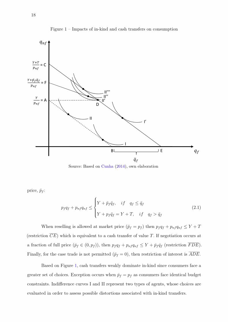
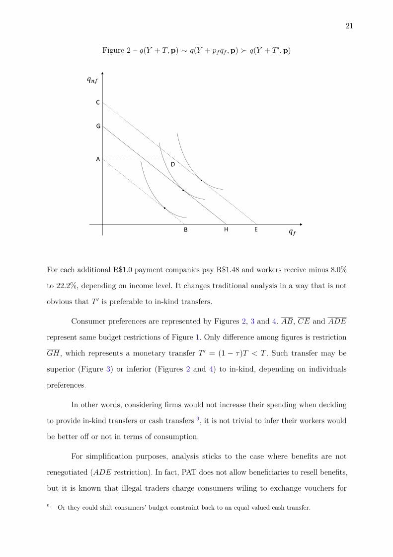
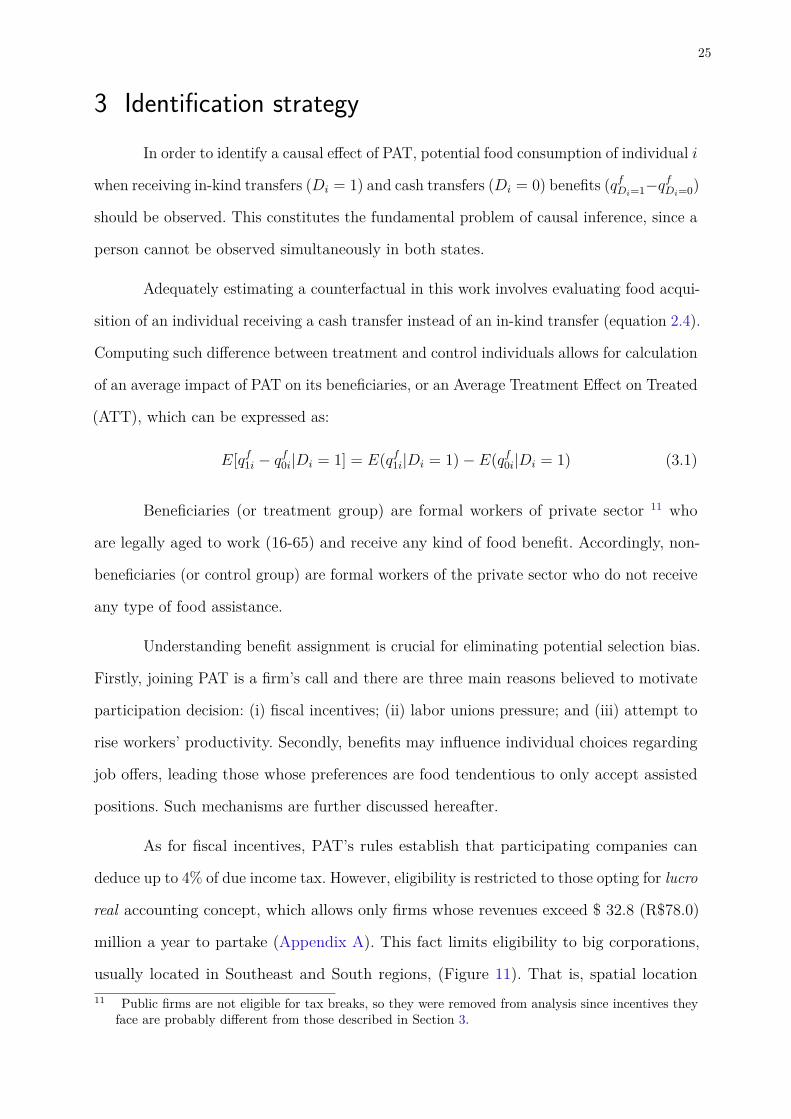
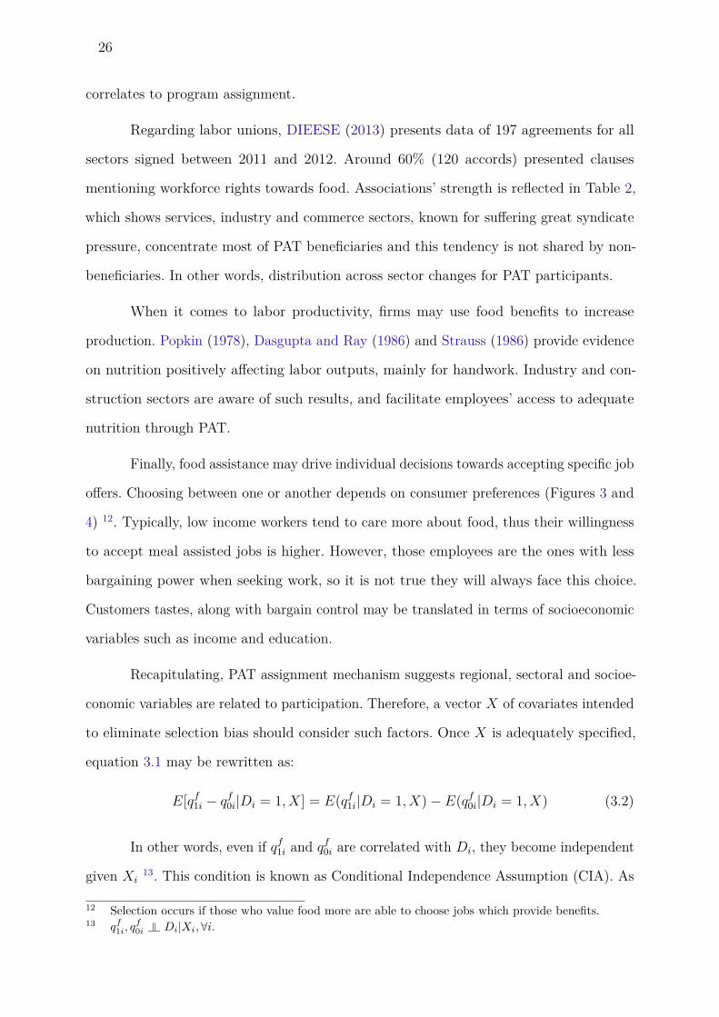
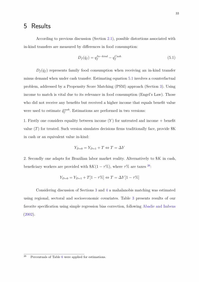
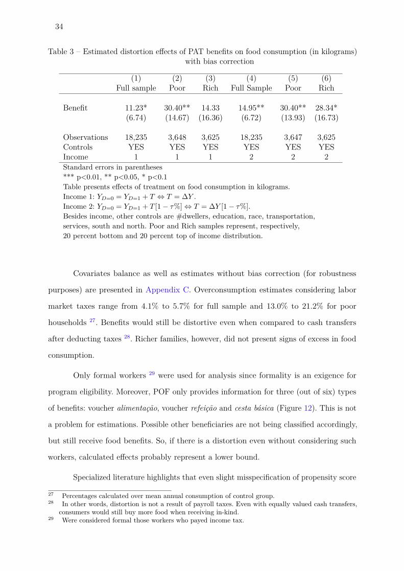

45
Figure 8 ndash Players interaction in meal voucher market Annual values in billion 2015 R$
Source Own elaborationIncludes meal voucher providers and companies which offer kitchen administration and
transported meal services
∙ Government Federal government is responsible for programrsquos existence It provides
tax breaks 39 of R$24 billion per year for companies willing to offer meal benefits
to its employees Such estimative was made using data from Ministry of Labor
IBGE and Brazilian Federal Revenue Office Total revenues were considered a sum
of average taxes payed from PAT and non-PAT companies Payments were adjusted
by company size
∙ Firms Are provided with tax breaks to offer food benefits 40 to its employees They
are allowed by law to charge their subordinates up to 20 of total value assistance 41
(around R$20 billion) Data from POF suggests companies charge only 314 on
average This percentage was multiplied by R$627 billion resulting in R$20 billion
39 Limited at 4 of due income tax40 Self-managed or outsourced41 For example R$100 transfers may be charged up to 20
46
∙ Service providers Companies specialized in restaurant administration in providing
transported meals andor meal vouchers 42 in form of debt cards They receive
variable fees 43 from firms for its services Market size was estimated in R$279 which
is a sum of percentages (4 and 5) received from firms (R$25 billion) restaurants
and supermarkets (R$31 billion) plus meal service provision 44 (R$222 billion)
∙ Workers Receive variable benefits 45 from firms (R$627 billion) and pay up to
20 46 the value of the benefit received They use their benefits in restaurants and
supermarkets that accept vouchers as payment methods 47 This value was estimated
considering an average payment received per employee (POF) times beneficiaries
number provided by Ministry of Labor
∙ Restaurants and supermarkets Sell food items to workers (R$627 billion 48) and
pay service providers a fee for all transactions made using its specific vouchers
There are other two effects worth mentioning One is taxes generated by food sector
which increases government collection They appear when voucher expending increment
sector turnover and when people are formally hired paying labor taxes Second is general
economy boost Food sector demands inputs from others 49 which are indirectly impulsed
and also generate taxes These effects can be assessed using traditional input-output
analysis
42 There is an association called Associaccedilatildeo das Empresas de Refeiccedilatildeo e Alimentaccedilatildeo Convecircnio para oTrabalhador (ASSERT) which represents 20 among biggest companies in this market Some famouscompanies are Alelo Sodexo Ticket and VR
43 For voucher provision firms are charged in 4 on average When it comes to restaurants andsupermarkets each debt pays around 5 Percentages were applied over R$627 billion to estimatemarket size which is probably underestimated
44 Calculated using minimal meal price per region from ASSERT research times number of workers(Ministry of Labor) and percentage of outsourced restaurants cesta baacutesica and transported meal insample
45 Federal government suggests firms should provide workers with balanced meals that meet min-imum nutritional requirements (for self-management) or minimum values allowing to buy foodin near restaurants (for meal vouchers) Official orientations from government regarding this is-sue were not found but Alelo releases a research with minimal and average meal values by statelthttpwwwvaloresminimospatcombrgt
46 Employers are free to decide whether workers pay any fee from 0 to 2047 Vouchers acceptance depends on bilateral agreements between service providers and establishments48 Considering workers spend all benefits received in both restaurants andor supermarkets49 eg agriculture oil amp gas (for plastic packing) transportation and others
47
BibliographyABADIE A IMBENS G SIMPLE AND BIAS-CORRECTED MATCHINGESTIMATORS FOR AVERAGE TREATMENT EFFECTS 2002 Disponiacutevel emlthttpwwwnberorgpaperst0283gt 33 63
ABADIE A IMBENS G W Large sample properties of matching estimators for averagetratment effects Econometrica v 74 n 1 p 235ndash267 2006 ISSN 0012-9682 63
ARAUacuteJO M d P N COSTA-SOUZA J TRAD L A B A alimentaccedilatildeo dotrabalhador no Brasil um resgate da produccedilatildeo cientiacutefica nacional Histoacuteria CiecircnciasSauacutede ndash Manguinhos v 17 n 4 p p975ndash992 2010 ISSN 0104-5970 Disponiacutevel emlthttpwwwscielobrpdfhcsmv17n408pdfgt 52
BANKS J BLUNDELL R LEWBEL A Quadratic Engel Curves and ConsumerDemand The Review of Economics and Statistics v 79 n 4 p 527ndash539 1997 40
BLUNDELL R PASHARDES P WEBER G What Do We Learn About ConsumerDemand Patterns from Micro Data The American Economic Review v 83 n 3 p570ndash597 1993 ISSN 00028282 Disponiacutevel em lthttpdiscoveryuclacuk15744gt 40
BRYSON A DORSETT R PURDON S The use of propensity score matching in theevaluation of active labour market policies 2002 57 p 27
BURLANDY L ANJOS L A D Acesso a vale-refeiccedilatildeo e estado nutricional de adultosbeneficiaacuterios do Programa de Alimentaccedilatildeo do Trabalhador no Nordeste e Sudeste doBrasil 1997 Cadernos de Sauacutede Puacuteblica v 17 n 6 p 1457ndash1464 2001 ISSN 0102-311X14
CAMPELLO T NERI M C Programa Bolsa Famiacutelia uma deacutecada de inclusatildeo ecidadania [Sl sn] 2013 502 p ISBN 9788578111861 17
CUNHA J M Testing Paternalism Cash versus In-Kind Transfers AmericanEconomic Journal Applied Economics v 6 n September p 195ndash230 2014 ISSN1945-7782 Disponiacutevel em lthttpsearchproquestcomdocview1511797736accountid=13042$delimiter026E30F$nhttpoxfordsfxhostedexlibrisgroupcomoxfordurl_ver=Z3988-2004amprft_val_fmt=infoofifmtkevmtxjournalampgenre=articleampsid=ProQProQeconlitshellampatitle=Testing+Patergt 1718 20 36
DASGUPTA P RAY D Inequality as a Determinant of Malnutrition and UnemploymentTheory The Economic Journal v 96 n 384 p 1011ndash1034 1986 26
DEATON A MUELLBAUER J An Almost Ideal Demand System The AmericanEconomic Review v 70 n 3 p 312ndash326 1980 40
DEHEJIA R H WAHBA S Causal effects in nonexperimental studies Reevaluatingthe evaluation of training programs Journal of the American statistical Association v 94n 448 p 1053ndash1062 1999 ISSN 0162-1459 27
DIEESE Relatoacuterio final sobre o Programa de Alimentaccedilatildeo do Trabalhador (PAT) [Sl]2013 223 p 26 51 52 55 56
48
GENTILINI U Cash and Food Transfers A primer Rome Italy 2007 34 p 17
GERALDO A P G BANDONI D H JAIME P C Aspectos dieteacuteticos das refeiccedilotildeesoferecidas por empresas participantes do Programa de Alimentaccedilatildeo do Trabalhador naCidade de Satildeo Paulo Brasil Revista Panamericana de Salud Puacuteblica v 23 n 1 p 19ndash252008 ISSN 1020-4989 14
HECKMAN J J ICHIMURA H TODD P Matching as an econometric evaluationestimator Review of Economic Studies v 65 p 261ndash294 1998 ISSN 0034-6527Disponiacutevel em lthttprestudoxfordjournalsorgcontent652261shortgt 27 28
HOYNES H W SCHANZENBACH D Consumption Responses to In-Kind TransfersEvidence from the Introduction of the Food Stamp Program American Economic JournalApplied Economics n 13025 p 109ndash139 2009 ISSN 1945-7782 13 35
IMAI K RATKOVIC M Covariate Balancing Propensity Score Journal of the RoyalStatistical Society v 76 p 243ndash263 2014 35
KANG J D Y SCHAFER J L Demystifying double robustness a comparisonof alternative strategies for estimating a population mean from incomplete dataStatistical Science v 22 n 4 p 523ndash539 2007 ISSN 0883-4237 Disponiacutevel emlthttparxivorgabs08042973gt 35
KEDIR A Health and productivity Panel data evidence from Ethiopia AfricanDevelopment Bank 2009 v 44 n 0 p 59ndash72 2009 13
KING G NIELSEN R Why Propensity Scores should not be used for matching 201528 63
MONCHUK V Reducing Poverty and Investing in People The New Role of Safety Netsin Africa [Sl] The World Bank 2014 165 p ISBN 9781464800948 13
MOURA J B de Avaliaccedilatildeo do do programa de alimentaccedilatildeo do trabalhador no Estadode Pernambuco Brasil Revista de Saude Publica v 20 n 2 p 115ndash128 1986 ISSN00348910 14
MTE PAT Responde 2015 Disponiacutevel em lthttpacessomtegovbrpatprograma-de-alimentacao-do-trabalhador-pathtmgt 52
NINNO C D DOROSH P Impacts of in-kind transfers on household food consumptionEvidence from targeted food programmes in Bangladesh [Sl sn] 2003 v 40 48ndash78 pISSN 0022-0388 13 36
PEREDA P Estimaccedilatildeo das equaccedilotildees de demanda por nutrientes usando o modeloQuadratic Almost Ideal Demand System (QUAIDS) 124 p Tese (Dissertaccedilatildeo de Mestrado)mdash Universidade de Satildeo Paulo 2008 40
PEREDA P C ALVES D C d O Qualidade alimentar dos brasileiros teoria eevidecircncia usando demanda por nutrientes Pesquisa e Planejamento Economico v 42n 2 p 239ndash260 2012 ISSN 01000551 38
PESSANHA L D R A experiecircncia brasileira em poliacuteticas puacuteblicas para a garantia dodireito ao alimento 2002 51
49
POI B Dairy policy and consumer welfare Tese (Doutorado) mdash Michigan University2002 40
POI B P Easy demand-system estimation with quaids Stata Journal v 12 n 3 p433ndash446 2012 ISSN 1536867X 40
POPKIN B M Nutrition and labor productivity Social Science amp Medicine v 12n 1-2 p 117ndash125 1978 26
RAY R Measuring the costs of children an alternative approach Journal of PublicEconomics v 22 p 89ndash102 1983 40
ROSENBAUM P R RUBIN D B The Central Role of the Propensity Score inObservational Studies for Causal Effects Biometrika v 70 n 1 p 41ndash55 1983 27
RUBIN D B Estimating causal effects of treatment in randomized and nonrandomizedstudies Journal of Educational Psychology v 66 n 5 p 688ndash701 1974 27
SAVIO K E O et al Avaliaccedilatildeo do almoccedilo servido a participantes do programa dealimentaccedilatildeo do trabalhador Revista de saude publica v 39 n 2 p 148ndash155 2005 ISSN0034-8910 14
SILVA A C da De Vargas a Itamar poliacuteticas e programas de alimentaccedilatildeo e nutriccedilatildeoEstudos Avanccedilados v 9 n 23 p 87ndash107 1995 52
SILVA M H O da Programa de Alimentaccedilatildeo do Trabalhador (PAT) Estudo dodesempenho e evoluccedilatildeo de uma poliacutetica social 145 p Tese (Dissertaccedilatildeo de Mestrado) mdashFundaccedilatildeo Oswaldo Cruz 1998 13 51
SKOUFIAS E UNAR M GONZAacuteLEZ-COSSIacuteO T The Impacts of Cash and In-KindTransfers on Consumption and Labor Supply Experimental Evidence from Rural Mexico2008 36
SMITH J A TODD P E Does matching overcome LaLondersquos critique ofnonexperimental estimators Journal of Econometrics v 125 p 305ndash353 2005 ISSN03044076 28 35
STRAUSS J Does better nutrition raise farm productivity Journal of Political Economyv 94 n 2 p 297ndash320 1986 26
VELOSO I S SANTANA V S Impacto nutricional do programa de alimentaccedilatildeo dotrabalhador no Brasil Revista Panamericana de Salud Puacuteblica v 11 n 1 p 24ndash31 2002ISSN 10204989 14
51
Appendix AA brief history of PAT
According to DIEESE (2013) Programa de Alimentaccedilatildeo dos Trabalhadores 50 (PAT)
creation took place in a wider context of food and nutrition programs in Brazil 51 Subject
became a concern during Getulio Vargas government (1934-1937) when malnutrition was
identified among Brazilian workers
Later during the 50s and 60s tendency continued A first version of Food National
Plan and North American Project for Food and Peace are some examples They counted
on external support usually provided by FAO through World Food Program (WFP)
(PESSANHA 2002)
Through the 70s Food and Agriculture Organization of the United Nations (FAO)
released statistics about calories and protein consumption of undeveloped countries
Government realized Brazilians living in northeast region had minimum acceptable calorie
patterns (SILVA 1998)
In order to revert situation Instituto Nacional de Alimentaccedilatildeo 52 (INAN) was
created in 1972 being responsible for development of a Programa Nacional de Alimentaccedilatildeo
e Nutriccedilatildeo 53 (PRONAN) As a result a set of ten programs were created each one
designed for different purposes and handed to diverse government departments PAT was
among them
Program was created on April 14119905ℎ 1976 through Law No 6321 regulated by
Decree No 5 of January 14119905ℎ 1991 and headed by Department of Labor PAT is a
federal government program of voluntary membership which grants tax breaks for firms
willing to provide nutritionally adequate food to low-income workers 54 PATrsquos objectives
50 Workers Food Program in a free translation51 To name a few programs created in the 40s Instituto de Tecnologia Alimentar in 1944 Conselho
Nacional de Alimentaccedilatildeo (CNA) in 1945 and Serviccedilo de Alimentaccedilatildeo da Previdecircncia Social (Saps) in1940 Saps was responsible for installing restaurants inside big firms and provide hot meals at lowcosts to small firms
52 National Institute of Alimentation in a free translation53 National Program of Food and Nutrition in a free translation54 Low-income workers are those who make less than five minimum wages per month Today minimum
52
are to improve nutritional status of low-income workers increasing their health 55 and
productivity (MTE 2015)
Program rapidly expanded through industrialized centers with Satildeo Paulo concen-
trating more than two thirds of all participating firms It started attending 08 million
workers in 1977 until reaching 78 million in 1992 (SILVA 1995)
During the 1990s most programs launched by PRONAN were already abandoned
Only PAT and Programa Nacional de Alimentaccedilatildeo Escolar 56 (PNAE) kept functional
both facing little changes According to Arauacutejo Costa-Souza and Trad (2010) these two
are at present food assistancersquos oldest programs in country (DIEESE 2013)
Facts and figures
Nowadays PAT provides food benefits for almost 20 million formal workers57 most
of them as in past still concentrated in Southeast region As for Figure 9 613 (121
million) of PAT workers are established in this region North and Midwest regions have
been showing a higher growth rate (Figure 10) but are far from reaching its relative
importance Moreover beneficiaries have been constantly increasing during last few years
It shows programrsquos relevance as a public policy
Figure 9 ndash Millions of formal workers receiving benefits from PAT by region
134143
153162
176183
190195 197
84 89 95 100 109 114 117 120 121
2324
26 2829 30 32 33 33
1617
1820
2122 23 24 24
0808
0910
1011
11 12 12
0404
0505
0606
07 07 07
00
50
100
150
200
00
50
100
150
200
250
2008 2009 2010 2011 2012 2013 2014 2015 Apr2016Southeast South Northeast Midwest North Total
Source Own elaboration Data retrieved from mtegovbr
wage in Brazil is R$88000 a month Approximately 83 of PAT beneficiaries earn less than this55 Reducing incidence of diseases related to food and nutrition56 National School Feeding Program in a free translation57 Bolsa Famiacutelia perhaps the most famous Brazilian assistance program reaches 139 million families
53
Figure 10 ndash Growth by region (Index 2008 = 100)
Source Own elaboration Data retrieved from mtegovbr
Analyzing PATrsquos beneficiaries relatively to eligible workers only confirms program
concentration As for Figure 11 more than 50 of Satildeo Paulo workers receive one or more
benefits from program Rio de Janeiro and Espiacuterito Santo have respectively 484 and
466 of its workers inside firms that joined the program No other state presents such
high participation rates Amazonas in North region reaches 387
Rules for companies to join and maintain program eligibility can be summarized as
follows
1 Only firms that use the lucro real 58 accounting concept are eligible for deduction
For this reason only firms whose annual gross revenue exceeds R$78 million can use58 Brazilian government allows three forms of income tax payment Lucro Real Lucro Presumido and
Simples Nacional Firms opting for Simples Nacional pay lowest taxes but its annual gross revenuecannot exceed R$36 million As for Lucro Presumido duties are intermediary but revenues cannotsurpass R$78 million Finally in case option is Lucro Real companies are charged with highest ratesChoosing between one or other concept is no trivial accounting decision and depends which sectorfirm belongs
54
Figure 11 ndash PAT workers in of eligible workers (2014)
387
121 133
144
308
313
279
466
279
138
368
217
25
248153277136
376
484
165
74
129
359
382
294
504
137
Source Own elaboration Data retrieved from mtegovbr
PATrsquos credits as tax breaks
2 Once participating firms caught hiring informal workers loose eligibility
3 Firms must prioritize workers who receive less than five minimum wages per month
(low income workers) Above this threshold it is not mandatory to provide benefits
and values cannot overpass those of smaller salariesrsquo
PAT generates credits that can be deducted from due income tax Deduced amount
(Y) is calculated as follows
55
∙ 119884 is defined as a benefit 59 cost times number provided
119884 = 119883 119876where X is cost per meal and Q total number of meals
provided by firm
∙ 119883 however is calculated beforehand by taking 15 of all expenses with benefits
119883 = 15 119879119862
119876where TC represents firmrsquos total cost with food benefits
However there is a rule to define 119883 value if 119883 lt 249 60 than set 119883 lt 249 but if
119883 ge 249 then set 119883 = 80 249 = 199 Finally there is a global limit deduction of 4
of due income tax (IT) In other words if 119884 le 4 119868119879 the amount to be deduced is 119884
but if 119884 gt 4 119868119879 deduction equals (4 119868119879 )
As an example suppose a company that provides 100 meals a month (119876 = 100)
for its workers at a total cost of 119877$20 per meal (119879119862 = 2000) In this case 119883 should
equals 0152000100 = 3 but as it exceeds 249 119883 = 199 So company is able to deduce
119884 = 100 199 = 119877$199 from due income taxes respecting the limit of 4 of its total
income tax 61
There is a lot involved in a firmrsquos decision to join PAT Accountability decisions 62
and possibility of tax deduction as mentioned above are two examples There are however
external factors like labor unions that may interfere in this process DIEESE (2013) presents
data regarding 197 union agreements signed between 2011 and 2012 Around 120 agreements
(609 of total) presented clauses regarding workersrsquo rights towards food For example
100 of transportation and urban industry constracts (35 in total) mentioned food59 For example a hot meal Each formal worker will get at least 20 of them per month60 Values in R$ of 201561 From a rational point of view a participating firm has incentives to reach maximum discount (4)
Suppose a company that does not bind deduction restriction It is optimum to exchange salary forbenefits until limit is achieved
62 Again only companies in lucro real regimen are eligible
56
Regarding program implementation DIEESE (2013) describes the two possible
ways
1 Self-management firm provides cooked or non-cooked meals (eg own restaurants
and cesta baacutesica)
2 Outsourcing firm delegates above-mentioned tasks to an specialized firm andor
provides debt cards or coupons that can only be exchanged for food items (meal vouchers 63)
There are no legal restrictions for companies providing more than one modality
of benefit For example firms may run a private restaurant deliver cestas baacutesicas every
month and also provide workers with meal vouchers Figure 12 shows that between 2008-15
more than 640 of beneficiaries received meal vouchers (alimentaccedilatildeo - 387 and refeiccedilatildeo
- 239) 98 received cestas baacutesicas and only 54 self-manage their benefits
Figure 12 ndash of benefits provided by modality
Source Own elaboration Data retrieved from mtegovbr
Incentives faced by firms and workers
This section analyzes firms and employees incentives in providing and receiving
benefits from PAT Besides tax breaks participant corporations have another advantage63 In Brazil meal vouchers are called vale-refeiccedilatildeo when used to buy food in restaurants and vale-
alimentaccedilatildeo when used in supermarkets
57
Transfers are not considered salary so there is no incidence of payroll taxes As it will be
shown below those can be a heavy burden
From workerrsquos point of view there are two disadvantages regarding assistance
First is that in case of vouchers expending is restricted to restaurants or supermarkets 64
Second is above mentioned charges of 20 over values provided
Therefore as there are advantages and disadvantages for both firms and individuals
in givingreceiving benefits it is not obvious they would like to enroll PAT In order to
clarify this issue analysis of payroll tax structure for companies and workers is assessed in
Table 6
First costs monthly incurred by Brazilian firms are detailed Most workersrsquo rights
in Brazil were established by president Getuacutelio Vargas in 1943 with Decree-Law No 5452
known as Consolidaccedilatildeo das Leis do Trabalho (CLT) Law stated that workers must receive
an extra payment by the end of each year named 13th salary Also during vacation
period which is also paid they should receive an additional 13 of their salaries called
constitutional allowance (abono constitucional)
Companies are also responsible for paying social contributions Fundo de Garantia
por Tempo de Serviccedilo 65 (FGTS) is a saving account monthly filled with 8 of workerrsquos
salary This personal account aims at providing them financial safety and equity liquidity
respectively in case of involuntary unemployment and realty acquisition Instituto Nacional
do Seguro Social 66 (INSS) represents Brazilian social security system for which firms must
pay 20 of employeesrsquo remuneration every month It assures minimum income flow in
cases of unemployment retirement maternity disablement and pension for family in case
of death FGTS and INSS are also calculated over 13119905ℎ salary and vacation period
There are other contributions such as accident insurance and aliacutequota de terceiros
a contribution to finance professional entities connected to labor unions in Brazil 67 They
64 For other modalities as self-managed refectories consumption is restricted to available goods in anspecific moment
65 Guarantee Fund for Employees66 National Institute for Social Security67 Senai Sesi Sesc Senac and others - also known as the S system
58
increase companiersquos costs in approximately 58 every month
59
Table 6 ndash Monthly tax incidence over companies and individuals in Brazil (2015 R$)
Salary considered 8800 16516 21179 25793 32888 42074 66638Bands for payroll tax in-cidence Below 139913 From 139913 to
190398From 190399 to233188
From 233189 to282665
From 282666 to375105
From 375106 to466375 Above 466375
Com
pany
cost
s 13119905ℎ salary 657 1376 1765 2149 2741 3506 555313 Vacation 219 459 588 716 914 1169 1851
FGTS 700 1468 1883 2293 2923 3740 5923INSS 1751 3670 4707 5732 7309 9350 14808
Others 457 958 1228 1496 1908 2440 3865Salary + taxes 11664 24447 31350 38179 48682 62279 98638
increase 480 480 480 480 480 480 480
Wor
ker
cost
s Income tax 00 00 160 506 1385 3105 9632INSS 630 1486 1906 2837 3618 4628 5130
Total costs 630 1486 2067 3344 5003 7734 14762Net income 7250 15029 19113 22449 27885 34340 51876 decrease -80 -90 -98 -130 -152 -184 -222
Table shows by income band estimated payroll taxes for Brazil both for companies and laborers Estimates consider average salary of each band
For lowest band minimum salary (R$88000) was considered From corporations point of view salary paid for any given band actually represents a
cost 48 higher Considering subordinates gross payment received is discounted at increasing rates which vary from 8 to 222 Averages may vary
according to economic sectors
Source Departments of Social Security and the Treasure and Decree-Law No 5452 May 1119904119905 1943 Own elaboration
60
So as for Table 6 payrolls increase companiesrsquo duties by approximately 48
Therefore an additional cash transfer of R$100 actually costs R$148 and does not vary
with income bands
For workersrsquos however duties do vary with salary level Income tax for example
starts with 0 aliquot for wages below US$80000 (R$190398) As income increases
contribution increases to 75 then doubles to 15 225 and finally 275 68 for those
whose earnings exceed US$195995 (R$466468)
Laborers also pay INSS Difference from firms lies on lower aliquots While compa-
nies pay a fixed 20 rate workers pay 8 if they make less than US$58786 (R$139912)
9 up to US$97978 (R$233188) and 11 until reaching US$195956 (R$466375)
Above this threshold contribution is fixed Thus when considering all taxes cash transfers
suffer deductions that vary from 8 to 22 depending on wage
Suppose a firm has got an extra R$100 to spend with one worker It has to decide
between two options First it is to raise workerrsquos salary in an amount that including 48
taxes results in expending R$100 Second give R$100 as food benefit Table 7 analyzes
costs incurred by firm in both cases
Table 7 ndash Firm costs to raise workerrsquos income through cash and food benefit
Benefit Cash
Value provided 100 676Taxes 0 48
Total costs 100 100
So from firmsrsquo point of view food benefits worth R$676 equal cash transfers of
R$100 Other costs of benefit providing are not considered such as 4 payment for meal
voucher companies On the other hand tax breaks firms are entitled to are also not being
taken into account As for previous discussion corporations can save a maximum of 4 in
income taxes Still this is arguably a valid approximation and salary raises are way more
costly than benefits
68 It is important to emphasize that once achieving a new band higher percentage is applied over thedifference between your new income and limit of previous band
61
Appendix BQuestionnaire 1 interviewed families to collect characteristics of the residence and
residents Residence information involves type (house apartment) situation (own home
or rent) material of floor and ceiling and utility services provision Resident information
aims at identifying dwellersrsquo characteristics such as condition (reference person spouse
son) sex age weight height education and skin color
Questionnaires 2 and 3 named POF2 and POF3 respectively bring information
about familiesrsquo purchases Expenses on non-food items are measured quarterly or monthly
by POF2 and comprehend utility expenses domestic fuels maintenance of house and
equipments construction equipment and furniture acquisition domestic services decora-
tion rent and taxes POF3 is measured weekly and focus on food items bought for the
house The detail level of information is high For example it is possible to identify a
family which bought 05 kilograms of cheese in a supermarket paying R$10 with a credit
card
Finally questionnaire 5 analyzes family membersrsquo income in a monthly basis
Analyzed variables include number of works weekly worked hours salary and benefits
deductions economic activity (agriculture industry) occupation (manager army forces
professional of arts) position (public or private sector rural) and investments
63
Appendix CResults and balance for favorite specification
Table 8 and Figure 13 present covariate balance and estimates without bias cor-
rection 69 for 119879 = Δ119884 Analogously Table 9 and Figure 14 present for 119879 = Δ119884 [1 minus 120591]
Matching procedure was mahalanobis (King and Nielsen (2015)) with replacement (Abadie
and Imbens (2002)) and standard errors calculated as in (Abadie and Imbens (2006))
69 That is traditional ATT
64
Table 8 ndash ATT for 119879 = Δ119884 - Quantity (annual kg per capita)
Treated Control Difference Bias
Full
sam
ple
ATT 3870 3645 2251 - Obs 3322 14913 - -
Log Income 07 07 - 08Education 83 83 - 01
Black 01 01 - 00Dwellers 36 36 - 03
Transport 01 01 - 00Services 01 01 - 00South 02 02 - 00North 01 01 - 00
20
poor
ATT 2810 2342 4677 - Obs 315 3333 - -
Log Income 06 06 - 03Education 61 60 - 28
Black 01 01 - 00Dwellers 48 48 - 24
Transport 00 00 - 00Services 01 01 - 00South 01 01 - 00North 01 01 - 00
20
rich
ATT 4902 4569 3332 - Obs 987 2638 - -
Log Income 08 08 - 18Education 105 105 - -08
Black 01 01 - 00Dwellers 30 30 - 05
Transport 01 01 - 00Services 02 02 - 00South 02 02 - 00North 01 01 - 00
plt01 plt005 plt001ATT shows mean differences between treated and control Obs presents number of observations Bias = Remaining percentage bias after matching procedures
65
Table 9 ndash ATT for 119879 = Δ119884 [1 minus 120591] - Quantity (annual kg per capita)
Treated Control Difference Bias
Full
sam
ple
ATT 3870 3661 2086 - Obs 3322 14913 - -
Log Income 07 07 - 04Education 83 83 - 00
Black 01 01 - 00Dwellers 36 36 - 04
Transport 01 01 - 00Services 01 01 - 00South 02 02 - 00North 01 01 - 00
20
poor
ATT 2827 2333 4942 - Obs 358 3289 - -
Log Income 06 06 - -13Education 62 61 - 29
Black 01 01 - 00Dwellers 47 47 - 22
Transport 01 01 - 00Services 01 01 - 00South 01 01 - 00North 01 01 - 00
20
rich
ATT 5012 4846 1655 - Obs 929 2696 - -
Log Income 08 08 - 18Education 106 106 - -09
Black 01 01 - 00Dwellers 30 30 - 08
Transport 01 01 - 00Services 02 02 - 00South 02 02 - 00North 01 01 - 00
plt01 plt005 plt001ATT shows mean differences between treated and control Obs presents number of observations Bias = Remaining percentage bias after matching procedures
66
Figure 13 ndash Log Income balance - 119879 = Δ119884
01
23
45
4 6 8 10 12Income
Treated Control
Figure 14 ndash Log Income balance - 119879 = Δ119884 [1 minus 120591]
01
23
45
4 6 8 10 12Income
Treated Control
67
Results and balance for iterative method
Table 10 shows bias corrected distortion considering iterative method Table 11 and
Figure 15 present covariate balance and estimates without bias correction 70 for 119879 = Δ119884
Analogously Table 12 and Figure 16 present for 119879 = Δ119884 [1 minus 120591]
Table 10 ndash Estimated distortion effects of PAT benefits on food consumption (inkilograms) with bias correction - iterative method
(1) (2) (3) (4) (5) (6)Full Sample Poor Rich Full Sample Poor Rich
Benefit 1535 4461 1810 1945 3670 2038(758) (1614) (1881) (755) (1505) (1894)
Observations 15859 3366 3091 15859 3361 3095Controls YES YES YES YES YES YESIncome 1 1 1 2 2 2Standard errors in parentheses plt001 plt005 plt01Table presents effects of treatment on food consumption in kilogramsIncome 1 119884119863=0 = 119884119863=1 + 119879 hArr 119879 = Δ119884 Income 2 119884119863=0 = 119884119863=1 + 119879 [1 minus 120591] hArr 119879 = Δ119884 [1 minus 120591]Besides income other controls are dwellers education race transportationservices south and north Poor and Rich samples represent respectively20 percent bottom and 20 percent top of income distribution
70 Or ATT
68
Table 11 ndash ATT for 119879 = Δ119884 - Quantity (annual kg per capita) - iterative method
Treated Control Difference Bias
Full
sam
ple
ATT 3955 3851 1044 - Obs 2654 11073 - -
Log Income 07 07 - 04Dwellers 35 35 - 03Industry 01 01 - 00
Construction 01 01 - 00Commerce 02 02 - 00Northeast 02 02 - 00Southeast 04 04 - 00
20
poor
ATT 2953 2407 5457 - Obs 341 2821 - -
Log Income 06 06 - -05Dwellers 46 46 - 08Industry 01 01 - 00
Construction 01 01 - 00Commerce 01 01 - 00Northeast 03 03 - 06Southeast 03 03 - 00
20
rich
ATT 5192 4981 2113 - Obs 656 1710 - -
Log Income 08 08 - 12Dwellers 28 28 - 00Industry 01 01 - 00
Construction 01 01 - 00Commerce 02 02 - 00Northeast 01 01 - 00Southeast 04 04 - -03
plt01 plt005 plt001ATT shows mean differences between treated and control Obs presents number of observations Bias = Remaining percentage bias after matching procedures
69
Table 12 ndash ATT for 119879 = Δ119884 [1 minus 120591] - Quantity (annual kg per capita) - iterative method
Treated Control Difference Bias
Full
sam
ple
ATT 3955 3658 2965 - Obs 2654 11073 - -
Log Income 07 07 - 04Dwellers 35 35 - 02Industry 01 01 - 00
Construction 01 01 - 00Commerce 02 02 - 00Northeast 02 02 - 00Southeast 04 04 - 00
20
poor
ATT 2923 2338 5852 - Obs 384 2775 - -
Log Income 06 06 - -07Dwellers 45 45 - 14Industry 01 01 - 00
Construction 01 01 - 00Commerce 01 01 - 00Northeast 03 03 - 05Southeast 03 03 - 00
20
rich
ATT 5232 4975 2565 - Obs 624 1752 - -
Log Income 08 08 - 12Dwellers 28 28 - 03Industry 01 01 - 00
Construction 01 01 - 00Commerce 02 02 - 00Northeast 02 02 - 00Southeast 04 04 - -03
plt01 plt005 plt001ATT shows mean differences between treated and control Obs presents number of observations Bias = Remaining percentage bias after matching procedures
70
Figure 15 ndash Log Income balance - 119879 = Δ119884 - iterative method
01
23
45
4 6 8 10 12Income
Treated Control
Figure 16 ndash Log Income balance - 119879 = Δ119884 [1 minus 120591] - iterative method
01
23
45
4 6 8 10 12Income
Treated Control
71
Food decomposition analysis robustness
Tables 13 presents average treatment effect on treated estimations of food decom-
position without bias correction Tables 14 and 15 respectively show covariates balance for
favorite specification and iterative method
Table 13 ndash ATT for 119879 = Δ119884 [1 minus 120591] - Quantity (annual kg per capita) - no biascorrection
Favorite specification Iterative method
Full
sam
ple
Cereal and pasta -417 -292Fruits and vegetables -356 096
Sugar and candies -123 -077MeatChickenFish -059 001
Nonalcoholic beverages 176 623Alcoholic beverages 193 096
Industrialized 390 268
20
poor
Cereal and pasta 1283 682Fruits and vegetables 809 256
Sugar and candies 038 -083MeatChickenFish 097 -037
Nonalcoholic beverages 525 1907Alcoholic beverages 034 099
Industrialized 677 1059
20
rich
Cereal and pasta -1178 -352Fruits and vegetables -448 -778
Sugar and candies -309 206MeatChickenFish -475 -562
Nonalcoholic beverages -094 862Alcoholic beverages 017 441
Industrialized 887 474plt01 plt005 plt001Table measures treatment effect on treated (in kilograms) consideringno bias correction for seven food categories Favorite specification includes dwellers education race transportation services south and northdummies Variables of iterative method are dwellers industry constructioncommerce northeast and southeast
72
Table 14 ndash Favorite specification - Balance for 119879 = Δ119884 [1 minus 120591]
Treated Control Bias
Full
sam
ple
Obs 3167 13797 -Log Income 07 07 04Education 83 83 00
Black 01 01 00Dwellers 36 36 04
Transport 01 01 00Services 01 01 00South 02 02 00North 01 01 00
20
poor
Obs 339 3091 -Log Income 06 06 -18Education 61 61 23
Black 01 01 00Dwellers 48 47 28
Transport 00 00 00Services 01 01 00South 01 01 00North 01 01 00
20
rich
Obs 884 2484 -Log Income 08 08 15Education 106 106 -08
Black 01 01 00Dwellers 31 30 07
Transport 01 01 00Services 02 02 00South 02 02 00North 01 01 00
plt01 plt005 plt001ATT shows mean differences between treated and control Obs presents number of observations Bias = Remaining percentage bias after matching procedures
73
Table 15 ndash Iterative method - Balance for 119879 = Δ119884 [1 minus 120591]
Treated Control Bias
Full
sam
ple
Obs 2501 10097 -Log Income 07 07 05
Dwellers 35 35 01Industry 01 01 00
Construction 01 01 00Commerce 02 02 00Northeast 02 02 00Southeast 04 04 00
20
poor
Obs 356 2566 -Log Income 06 06 03
Dwellers 45 45 17Industry 01 01 00
Construction 01 01 00Commerce 01 01 00Northeast 04 04 06Southeast 03 03 00
20
rich
Obs 579 1593 -Log Income 08 08 16
Dwellers 28 28 00Industry 01 01 00
Construction 01 01 00Commerce 02 02 00Northeast 02 02 00Southeast 04 04 -04
plt01 plt005 plt001ATT shows mean differences between treated and control Obs presents number of observations Bias = Remaining percentage bias after matching procedures
- Title page
- Dedication
- Agradecimentos
- Epigraph
- Resumo
- Abstract
- List of Figures
- List of Tables
- Contents
- Introduction
- In-kind transfers
-
- In-kind versus cash transfers
- Brazilian context
-
- Identification strategy
- Dataset
- Results
- Welfare considerations
- Remarks and policy considerations
- Bibliography
- Appendix A
- Appendix B
- Appendix C
-
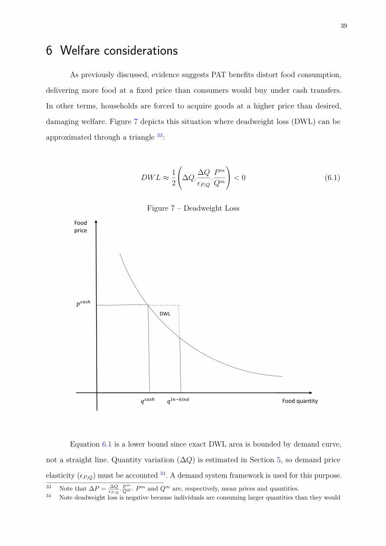
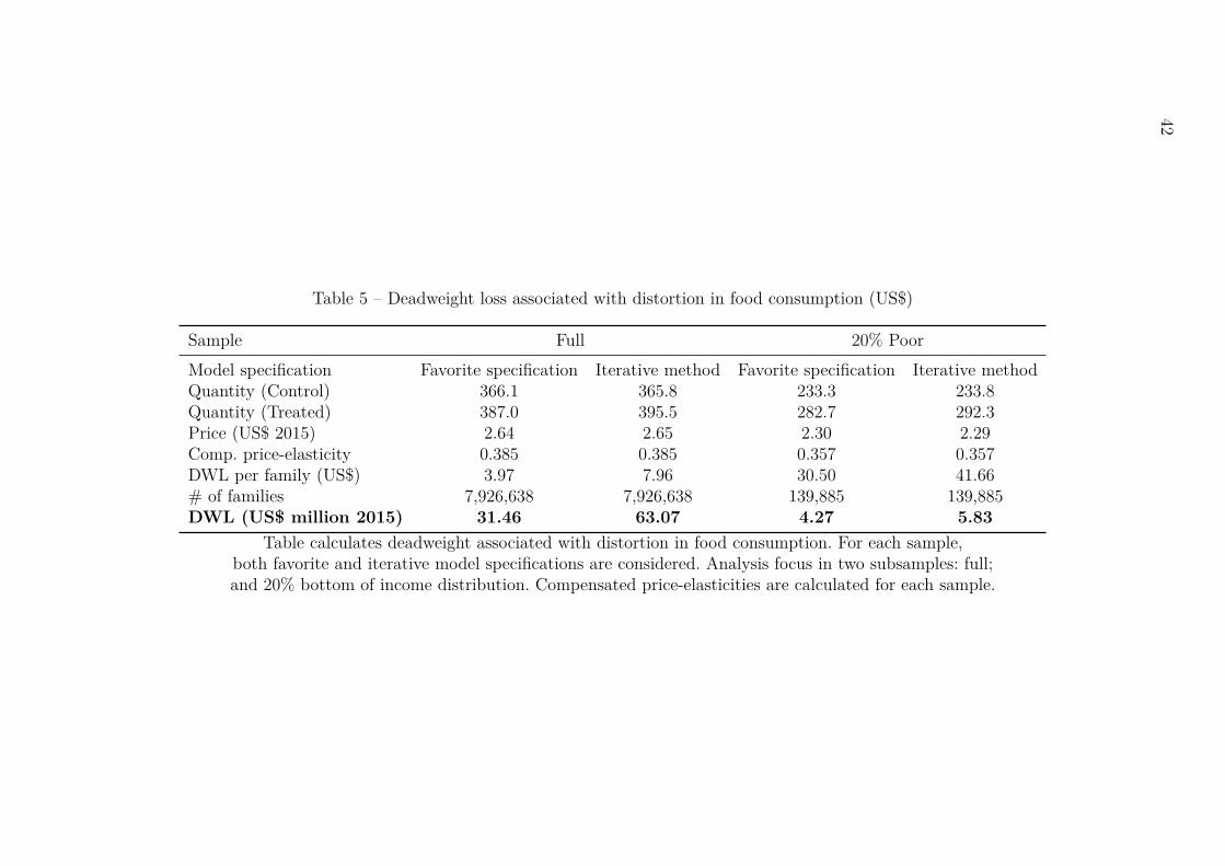
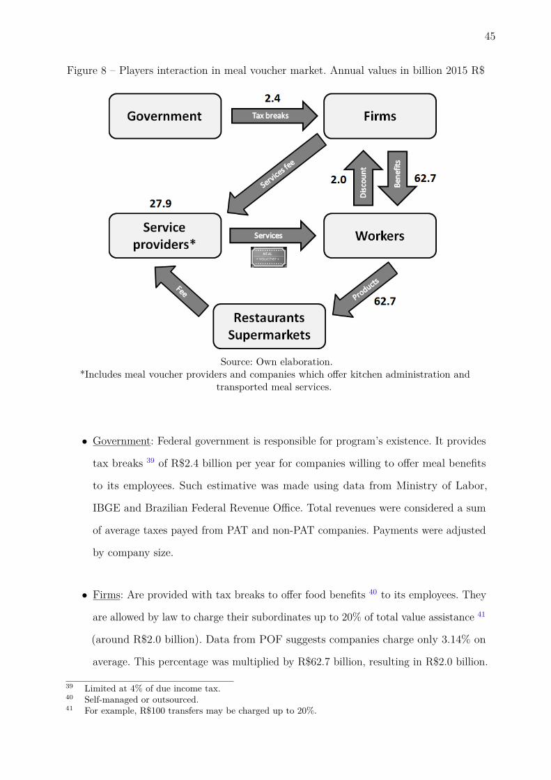
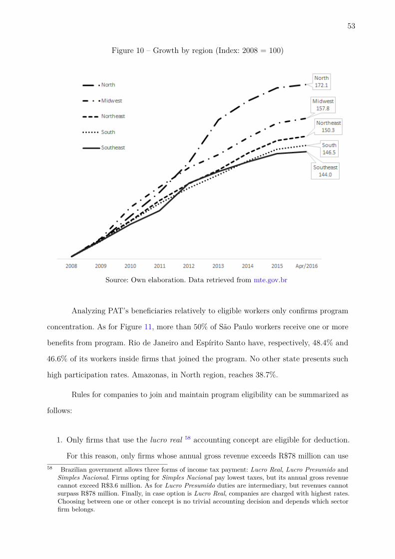
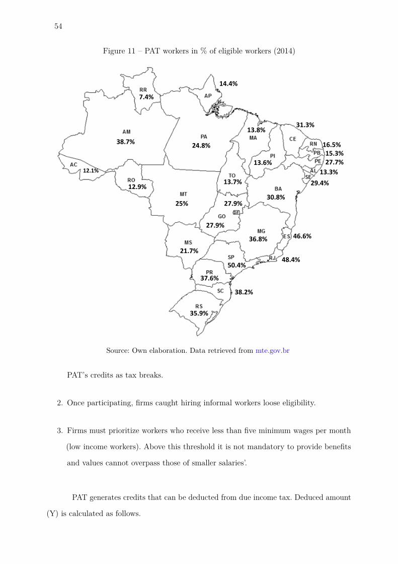