in copyright - non-commercial use permitted rights ...8703/eth... · pascal rolli msc eth...
TRANSCRIPT

Research Collection
Doctoral Thesis
Split quasicocycles and defect spaces
Author(s): Rolli, Pascal
Publication Date: 2014
Permanent Link: https://doi.org/10.3929/ethz-a-010168196
Rights / License: In Copyright - Non-Commercial Use Permitted
This page was generated automatically upon download from the ETH Zurich Research Collection. For moreinformation please consult the Terms of use.
ETH Library

DISS. ETH Nr. 21792
SPLIT QUASICOCYCLES AND DEFECT SPACES
A thesis submitted to attain the degree of
DOCTOR OF SCIENCES of ETH ZURICH
(Dr. sc. ETH Zurich)
presented by
PASCAL ROLLI
MSc ETH Mathematics, ETH Zurich
born on 30.06.1985
citizen of Oberbalm BE
accepted on the recommendation of
Prof. Dr. Alessandra Iozzi, examiner
Prof. Dr. Sebastian Baader, co-examiner
Prof. Dr. Koji Fujiwara, co-examiner
2014


Fur d’JasminFure Urs


Bi erwachet hut am Morge
Da woni geschter scho bi gsi
Ir Mitti vomne Schrottplatz
Wi dr Esu vorem Barg
. . .
(Hotelsong)


Abstract
Let Γ be a group. A map Γ −→ E, ranging in a Banach Γ-module E, is called aquasicocycle if it satisfies the cocycle identity up to bounded error. To a quasicocy-cle one associates a class in the second bounded cohomology H2
b(Γ, E). The authorhas previously observed (see [47]) that for a free product of groups Γ = A ∗B, anygiven pair of alternating quasicocycles on the factors A,B can be extended to whatwe call a split quasicocycle on the whole group Γ. This thesis is concerned withthe study of split quasicocycles and their significance for bounded cohomology.
Under mild assumptions on the factors of Γ = A ∗ B, we prove that the splitquasicocycles yield infinite dimensional subspaces of H2
b(Γ, E) whenever the coef-ficient module E is finite-dimensional or of the type ℓp(Γ) for 1 ≤ p <∞.
In the case E = R we are dealing with split quasimorphisms. Here we show thatevery cohomology class obtained from our construction has Gromov norm equalto one half of the defect of the homogenous quasimorphism representing it. Thisproperty is known to hold for Brooks’ counting quasimorphisms and it is an openquestion whether it holds in general. We identify the induced subspace of H2
b(Γ,R)to be built up from isometrically embedded defect spaces. The defect space D(H)of a group H is introduced as the space of alternating bounded functions H −→ R,equipped with an certain exotic norm called the defect norm.
Since the geometry of the space H2b is poorly understood we are motivated to
study the geometry of defect spaces. It turns out that the set of extremal pointsin the closed unit ball of D(H) encodes different properties of the group H. Forexample, we find a subset of extremal points that is naturally homeomorphic toSikora’s space of left-orders on H.
For the case of a free group, we construct split quasimorphisms that vanish ona given subgroup of infinite index. As a result we obtain embeddings of defectspaces into the relative second bounded cohomology. This part is based on jointwork with Cristina Pagliantini.
We suggest furthermore a new geometric construction of a quasimorphism onthe free group, based on the CAT(0) geometry of a polygonal complex quasi-isometric to the group’s Cayley graph. This construction turns out to admit ageneralization which also encompasses split quasimorphisms.
Replacing the target space E with a metric group yields a new type of quasi-representations whose construction is much clearer than it is the case for thepreviously known examples due to Kazhdan (see [36]).


Zusammenfassung
Es sei Γ eine Gruppe. Eine Abbildung Γ −→ E in einen Banach Γ-modul Eheisst Quasikozykel, wenn sie die Kozykelidentitat bis auf einen beschranktenFehler erfullt. Zu einem Quasikozykel assoziiert man eine Klasse in der zweitenbeschrankten Kohomologie H2
b(Γ,R). Der Autor hat bereits fruher festgestellt(siehe [47]), dass fur ein freies Produkt Γ = A ∗ B jedes gegebene Paar al-ternierender Quasikozykel auf den Faktoren A,B zu einem sogenannten gespalte-nen Quasikozykel auf der ganzen Gruppe Γ fortgesetzt werden kann. Diese Arbeitbefasst sich mit dem Studium der gespaltenen Quasikozykel und deren Bedeutungfur die beschrankte Kohomologie.
Unter schwachen Bedingungen an die Faktoren A,B zeigen wir das gespalteneQuasikozykel unendlich-dimensionale Unterraume von H2
b(Γ, E) ergeben, falls derKoeffizientenmodul E endlich-dimensional ist, oder vom Typ ℓp(Γ), 1 ≤ p <∞.
Im Fall E = R haben wir es mit gespaltenen Quasimorphismen zu tun. Hierzeigen wir, dass fur jede der induzierten Kohomologieklassen die Gromov-Normubereinstimmt mit dem halben Defekt des homogenen Quasimorphismus, der die-selbe Klasse reprasentiert. Diese Eigenschaft haben auch die Zahlquasimorphismenvon Brooks, und es ist eine offene Frage ob sie allgemein gilt. Wir identifizierenden zughorigen Unterraum von H2
b(Γ,R) als Summe von isometrisch eingebettetenDefektraumen. Den Defektraum D(H) einer Gruppe H fuhren wir ein als Raumder alternierenden beschrankten Funktionen H −→ R, ausgestattet mit einer exo-tischen Norm, der Defektnorm.
Uber die Geometrie des Raumes H2b weiss man erst wenig, und dies motiviert
uns, die Geometrie der Defektraume zu untersuchen. Es stellt sich heraus, dassdie Menge der Extremalpunkte im abgeschlossenen Einheitsball von D(H) ver-schiedene Eigenschaften der Gruppe H kodiert. Beispielsweise bestimmen wir eineTeilmenge der Extremalpunkte, die auf naturliche Weise homoomorph zu SikorasRaum der Linksordnungen auf H ist.
Fur den Fall einer freien Gruppe konstruieren wir gespaltene Quasimorphismen,die auf einer gegebenen Untergruppe mit unendlichem Index verschwinden. Darauserhalten wir Einbettungen von Defektraumen in die relative zweite beschrankteKohomologie. Dies basiert auf einer Zusammenarbeit mit Cristina Pagliantini.
Weiter prasentieren wir eine neue geometrische Konstruktion eines Quasimor-phismus auf der freien Gruppe, basierend auf der CAT(0)-Geometrie eines polygo-nalen Komplexes, der zum Cayley-Graph der Gruppe quasiisometrisch ist. Es zeigtsich, dass diese Konstruktion eine gemeinsame Verallgemeinerung mit gespaltenenQuasimorphismen besitzt.
Indem wir den Modul E durch eine metrische Gruppe ersetzen, erhalten wirneue Quasi-Darstellungen, deren Konstruktion viel klarer ist als es bei den bekan-nten Beispielen von Kazhdan (siehe [36]) der Fall ist.


Danksagung
Mein grosster Dank gilt Alessandra Iozzi, meiner Betreuerin. Sie hat mich wahrendder letzten Jahre stets mit wertvollem Rat unterstutzt, hat mich an interessanteThemen herangefuhrt und mir den Austausch mit vielen Mathematikern ermoglicht.Ich schatze es sehr, dass sie mir bei der Gestaltung meines Doktorats viele Frei-heiten gelassen hat. Ihren ausserordentlichen Optimismus und ihre “Can do”–Einstellung nehme ich mir als Beispiel!
Weiter danke ich Marc Burger fur seine zahlreichen Anregungen, insbesonderefur den Vorschlag Defektraume zu untersuchen, meinen Korreferenten SebastianBaader und Koji Fujiwara fur ihre nutzlichen Bemerkungen zu dieser Dissertationund Cristina Pagliantini fur die fruchtbare Zusammenarbeit.
Beatrice Pozzetti und Theo Buhler haben mir detaillierte Ruckmeldungen zuTeilen dieser Arbeit geliefert, wofur ich sehr dankbar bin. Ebenso waren mirdie Erlauterungen von Danny Calegari uber die Gromov-Norm der Zahlquasi-morphismen hilfreich.
Meinen Kollegen danke ich fur viele Diskussionen und die angenehme Atmo-sphare wahrend der gemeinsam verbrachten Zeit. Es sind dies, in der Reihenfolgeihres Auftretens: Thomas Huber, Tobias Strubel, Tobias Hartnick, Roger Zust,Alex Maier, Maria Hempel, Christian Lieb, Beatrice Pozzetti, Claire Burrin, Stef-fen Weil, Waltraud Lederle, Stephan Tornier, Carlos de la Cruz und AlessandroSisto.
Schliesslich danke ich auch Mami, Marvin und meiner lieben Risa.
Rolle, im Fruhling 2014


Contents
Introduction 1
1 Preliminaries 9
1.1 Quasicocycles and bounded cohomology . . . . . . . . . . . . . . . 9
1.2 Relative quasicocycles and bounded cohomology . . . . . . . . . . . 12
2 Split quasicocycles 15
2.1 Finite-dimensional coefficients . . . . . . . . . . . . . . . . . . . . . 16
2.2 ℓp-coefficients . . . . . . . . . . . . . . . . . . . . . . . . . . . . . . 18
3 Split quasimorphisms 21
3.1 Embedding defect spaces . . . . . . . . . . . . . . . . . . . . . . . . 21
3.2 Amalgamated products . . . . . . . . . . . . . . . . . . . . . . . . . 24
3.3 Actions of automorphisms . . . . . . . . . . . . . . . . . . . . . . . 26
3.4 A relation to counting quasimorphisms . . . . . . . . . . . . . . . . 29
4 Split quasi-representations 32
5 Geometric deformation quasimorphisms 34
6 A common generalization of split and deformation QMs 40
6.1 The construction . . . . . . . . . . . . . . . . . . . . . . . . . . . . 40
6.2 Examples . . . . . . . . . . . . . . . . . . . . . . . . . . . . . . . . 42
6.3 Computing the Gromov norm . . . . . . . . . . . . . . . . . . . . . 44
7 Defect spaces 47
7.1 Definition and first properties . . . . . . . . . . . . . . . . . . . . . 47
7.2 Existence of extremal points . . . . . . . . . . . . . . . . . . . . . . 50
7.3 Extremal points for finite groups . . . . . . . . . . . . . . . . . . . 53
7.4 Left orders and extremal points with maximal sup-norm . . . . . . 53
7.5 Extremal points from quotients . . . . . . . . . . . . . . . . . . . . 57
7.6 Extremal points from infinite chains of normal subgroups . . . . . . 59
7.7 Extremal points with minimal sup-norm . . . . . . . . . . . . . . . 62
7.8 Extremal points from the circle group . . . . . . . . . . . . . . . . . 64
7.9 Higher defect spaces . . . . . . . . . . . . . . . . . . . . . . . . . . 66
8 Relative bounded cohomology of free groups 67
9 Quasimorphisms induced from hyperbolic mapping tori 72
Appendix: H2b(F2,R) is infinite dimensional, a simple proof 77
References 78


1
Introduction
Let Γ be a group and let E be a Banach Γ-module, that is, a Banach space endowedwith a linear isometric Γ-action. Recall that f : Γ −→ E is called a cocycle if themap
∂f : (g, h) 7→ f(g)− f(gh) + g.f(h)
vanishes identically on Γ × Γ. If Γ acts trivially on E then cocycles are homo-morphisms. If ∂f has bounded range then f is called a quasicocycle, or, in thecase E = R, a quasimorphism. Bounded perturbations of cocycles are obviouslyquasicocycles, and it turns out that a quasicocycle f : Γ −→ E is of this trivialtype, if and only if it is contained in the kernel of the map
QZ(Γ, E) −→ H2b(Γ, E)
which associates to f the class [∂f ]b in the second bounded cohomology of Γ withcoefficients in E.
The standard example is the counting quasimorphism Cw : F2 = ⟨a, b⟩ −→ Rof Brooks, defined on the rank two free group (see [14]). This simple construc-tion has a word w ∈ F2 as its parameter. To determine the value Cw(g) onecounts in g the number of subwords equal to w, and subtracts the correspondingnumber for the inverse word w−1. As soon as w has length at least two, Cw is non-trivial. Mitsumatsu showed, by varying the parameter w, that the cohomologyclasses associated to counting quasimorphisms span an infinite dimensional sub-space in H2
b(F2,R) (see [40]). Epstein and Fujiwara defined generalized countingquasimorphisms for word-hyperbolic groups and showed that the second boundedcohomology of such a group has infinite dimension (unless the group is elemen-tary). A further generalization for groups acting properly on Gromov-hyperbolicspaces was given by Fujiwara (see [26]), and Bestvina–Fujiwara showed that itis sufficient to have an action which is weakly proper (see [9]). This last resultincludes the notable case of the mapping class group acting on the curve complex.
Barge–Ghys defined a quasimorphism of different nature for the fundamentalgroup Γ of a closed negatively curved manifold M (see [4] and also the discussionin [19], Section 2.3.1). The parameter of their quasimorphism fλ : Γ −→ R is adifferential 1-form λ on M . For g ∈ Γ, the value fλ(g) is defined to be the integralof λ along the unique geodesic loop representing g. Using this construction in thecase of surfaces they characterized metrics of constant negative curvature via thearea of ideal triangles ([4], Theoreme 3.11).
In all these examples we have an infinite dimensional space H2b. On the other
hand, the bounded cohomology of amenable groups vanishes, as was shown byJohnson (see [35]). This means that on such a group every quasimorphism istrivial. By the work of Burger–Monod this property holds as well for higher rank

2
lattices ([15], Corollary 1.3), a fact which they used to establish rigidity resultsfor actions of lattices on the circle. Bestvina–Fujiwara combined this with theirconstruction mentioned above, leading to a new proof of a rigidity statement forrepresentations of lattices into mapping class groups ([9], Corollary 13).
The (non-)existence of non-trivial quasimorphisms has an impact also in thetheory of stable commutator length (scl): Bavard proved that the scl functionof a group is identically equal to zero, if and only if every quasimorphism onthis group is trivial ([6], Corollaire 1). Moreover, in case scl does not vanish, itcan be expressed through quasimorphisms by means of Bavard’s duality theorem([6], Theoreme de dualite, p.141). A large number of further results connectingquasimorphisms and scl is found in Calegari’s monograph on the topic (see [19]).
A further area in which quasimorphisms have been studied is measured grouptheory, notably in the work of Bjorklund–Hartnick on central limit theorems forquasimorphisms (see [11]). In symplectic topology quasimorphisms have beenpresent since the work of Entov–Polterovich (see [22]). In a rather curious wayquasimorphisms on the integers were used by A’Campo for a new construction ofthe real number system (see [1]).
Among the quasicocycles with non-trivial target, those ranging in the left-regular representation have found particular attention. For groups Γ acting onGromov hyperbolic graphs, Monod–Mineyev–Shalom have constructed non-trivialquasicocycles Γ −→ ℓp(Γ) for 1 ≤ p < ∞ (see [39]). These groups satisfy in par-ticular H2
b(Γ, ℓ2(Γ)) = 0, a property which by the work of Monod-Shalom is an
invariant of measure equivalence, and is thought of as a cohomological character-ization of negative curvature of a group (see [43] and [44]). On a more generallevel, Hamenstadt used boundary theory to construct ℓp-valued quasicocycles forgroups which admit a weakly proper action on an arbitrary Gromov hyperbolicspace (see [31]). A further generalization was obtained by Hull–Osin, who gave aconstruction of ℓp-quasicocycles for groups that contain a hyperbolically embeddedsubgroup (see [33]).
Targets other than left-regular representations have been studied as well. Arecent example is found in the construction of a distinguished bounded cohomologyclass for a group acting on a CAT(0) cube complex X, due to Chatterji–Fernos–Iozzi (see [20]). Here the coefficients are of a geometric type, they are defined usingthe halfspace structure of X. A construction with very general coefficients hasbeen carried out by Bestvina–Bromberg–Fujiwara (see [8]). Their quasicocyclesare defined on groups Γ that act on a geodesic metric space, where at least onegroup element needs to show a “rank 1” behavior. Here the coefficients are anarbitrary uniformly convex Banach module E, for example a module of finitedimension. This construction is inspired by Brooks counting quasimorphisms, andit yields an infinite dimensional space H2
b(Γ, E).
3
Let now Γ be a group and let E be a Banach Γ-module. Assume that we have asplitting Γ = A∗B of our group into a free product. A cocycle Γ −→ E is uniquelydetermined by its restrictions to the free factors A and B, and in fact, every pairof cocycles
fA : A −→ E, fB : B −→ E
extends in a unique way to a cocycle on Γ. This fact is no longer true if weconsider quasicocycles. However, given two alternating quasicocycles fA and fBthere is still a natural way of defining an extension f : Γ −→ E:
f(a1b1 . . . anbn) :=
fA(a1) + a1.fB(b1) + a1b1.fA(a2) + · · ·+ a1b1a2 · · · bn−1an.fB(bn).
We write f = fA ∗ fB for this extension and call it a split quasicocycle. Thisformula appeared in the author’s master thesis (see [47], Remark (iii), p.5), and itwas discovered independently by Thom (see [55], Lemma 5.1). By what we saidabove, f is trivial iff the pair (fA, fB) belongs to the kernel of the map
Φ : QZalt(A,E)×QZalt(B,E) −→ H2b(Γ, E),
(fA, fB) 7→ [∂(fA ∗ fB)]b.
We refer to the image of Φ as the space of split classes, and we prove that undersuitable assumptions this space is infinite dimensional:
Theorem 2.3. Let Γ be a finitely generated group with a splitting Γ = A ∗ B,such that A contains an element of infinite order. Then for any finite dimensionalBanach Γ-module E the split classes form an infinite dimensional subspace ofH2
b(Γ, E).
Under essentially the same assumptions on Γ we have
Theorem 2.5. Let Γ be a countable group with a splitting Γ = A ∗ B, such thatA contains an element of infinite order. For 1 < p <∞ the split classes form aninfinite-dimensional subspace of H2
b(Γ, ℓp(Γ)). If the factor A is amenable then the
same holds for p = 1.
These statements apply in particular in the situation A = B = Z, i.e. when Γ isfree of rank two. We note that infinite-dimensionality of the spaces H2
b(Γ, E) in theabove theorems also follows from the work of Hull–Osin in the case of ℓp-coefficients(see [33], Corollary 1.7), and from the work of Bestvina–Bromberg–Fujiwara in thefinite dimensional case (see [8], Theorem 5.1). Let us now consider the case of thetrivial target E = R. Here we obtain split quasimorphisms from a given splittingΓ = A ∗B, and we identify the kernel of the corresponding map
Φ : QMalt(A)×QMalt(B) −→ H2b(Γ,R)
as the subspace Hom(A,R)× Hom(B,R). More precisely:

4
Theorem 3.3. Let f = fA ∗ fB be a split quasimorphism with corresponding co-homology class ωf = [∂f ]b. We have
∥ωf∥ = 12def f = def f = max{def fA, def fB}.
In particular, f is a minimal defect representative for its class.
Here ∥ · ∥ stands for the Gromov norm on the space H2b(Γ,R), and for a quasi-
morphism f we denote by f its homogenization and by def f its defect (see sub-section 1.1). Among other things this theorem implies that a split quasimorphismf = fA ∗ fB is non-trivial as soon as one of the factors fA,fB is not a homomor-phism. Therefore we get a linear embedding ℓ∞alt(A) × ℓ∞alt(B) ↪−→ H2
b(Γ,R). Thespaces ℓ∞alt of alternating bounded functions on the respective groups are Banach,and so is the space H2
b(Γ,R) when equipped with the Gromov norm. This leadsto the question whether the embedding under consideration respects the involvednorms in any way. To give a precise answer we introduce the notion of the defectspace of a group H. This is the space
D(H) := {f : H −→ R | f is bounded and alternating}
equipped with the norm
∥f∥def := def f = supg,h∈H
|f(gh)− f(g)− f(h)|.
Using this definition we obtain
Theorem 3.6. For a group Γ = A ∗B there is a linear isometric embedding
D(A)⊕∞ D(B) ↪−→ H2b(Γ,R)
which maps the pair (fA, fB) to the bounded cohomology class ωf of the split quasi-morphism f = fA ∗ fB.
Here the symbol ⊕∞ stands for the max-norm on the sum of two Banach spaces.The previous two theorems imply in particular that for every cohomology class ωf
in the embedded space D(A)⊕D(B) the Gromov norm satisfies
∥ωf∥ = 12def f .
It is an open question whether this equality holds in general for the class of aquasimorphism. Through Bavard’s duality theorem a positive answer to this ques-tion would provide a link between commutator geometry and the geometry of thespace H2
b (see the discussion in [19]). Equality was shown for a single example of
5
a counting quasimorphism by Bavard ([6], p.148), and Calegari established it forall counting quasimorphisms and their finite linear combinations (see [18]).
The defect space D(H) has the same underlying vector space as ℓ∞alt(H) andin fact these spaces are norm-equivalent: We have ∥f∥∞ ≤ ∥f∥def ≤ 3∥f∥∞ forany bounded alternating function f on H. Since the geometry of the H2
b is poorlyunderstood we are motivated to study the geometry of defect spaces; we are alsonot aware of any previous discussion of these spaces. We observe that D(H) is adual Banach space and, as such, it has a non-empty set of extremal points E(H) inits closed unit ball. This is obvious in the case of a finite group H where the unitball is a polytope. We show that several properties of the group H are reflectedin the set E(H). Most notably, we identify a certain subset E1(H) ⊂ E(H) suchthat to each function f ∈ E1(H) we can associate a total left-invariant order ≤f
on the group H. The assignment f 7→≤f has a naturally defined inverse. Moreprecisely we have the following result in which LO(H) stands for Sikora’s space ofleft-orders on H (see [50]):
Corollary 7.22. If we endow the set E1(H) with the topology induced from theweak*-topology on D(H) then the map
E1(H) −→ LO(H), f 7→ ≤f
is a homeomorphism.
Another result of this type concerns a subset E∗(−1,1)(H) ⊂ E(H) which detectsembedings of H into the circle group T:
Theorem 7.32. For every group H there is a natural correspondence
{embeddings H ↪−→ T} ←→ E∗(−1,1)(H)
This correspondence yields infinitely many points in E(Z) which, as functionsZ −→ R, only take irrational values. The next result shows that the set of extremalpoints contains the extremal points for the quotients of our group:
Theorem 7.24. For a short exact sequence
1 // N // H // Q // 1
in which the group Q is 2-torsion free, we have an induced embedding
j : D(N)⊕∞ D(Q) ↪−→ D(H)
which maps extremal points to extremal points. That is, we have an embedding
E(N)× E(Q) ↪−→ E(H).

6
For the group Z this result can be used to obtain extremal points which haveboth rational and irrational values. The next statement yields points in E(Z)which are purely rational but non-periodic:
Corollary 7.29. If the countably infinite group H is residually finite 2-torsionfree, then its set of extremal points E(H) contains uncountably many rational-valued functions.
We show that defect spaces are also found as isometric subspaces of relativebounded cohomology. Let H be a subgroup of a group Γ. We say that f :Γ −→ R is a relative quasimorphism for the pair (Γ, H) if it is a quasimorphismwith f |H ≡ 0. To such a map one has an associated class in the relative secondbounded cohomology H2
b(Γ, H;R) (see subsection 1.2). Using the construction ofsplit quasimorphisms, we proved the following result in joint work with CristinaPagliantini (see [45]):
Theorem 8.1. Let Γ be a free group of finite rank n ≥ 2, and let H < Γ be asubgroup of finite rank. The following are equivalent
(i) H has infinite index in Γ,
(ii) The space H2b(Γ, H;R) is non-trivial.
(iii) There exists a linear isometric embedding
⊕n∞D(Z) ↪−→ H2
b(Γ, H;R)
The crucial step in the proof of this statement is the construction of a suitablebasis of Fn, namely of a basis that admits split quasimorphisms which vanish onthe subgroup H. This is accomplished through the following lemma which may beof independent interest:
Lemma 8.2. Let Γ be a free group of finite rank n ≥ 2 and let H < Γ be a subgroupof finite rank and infinite index. There exists a basis {x1, . . . , xn} of Γ such thatfor all g ∈ Γ and for all i we have
gHg−1 ∩ ⟨xi⟩ = {e},
which is to say that no conjugate of H contains a power of an element of this basis.
For a group Γ and a metric group (G, d), a map µ : Γ −→ G is called aquasi-representation (or ε-representation) if the expression d(µ(gh), µ(g)µ(h)) isuniformly bounded. This notion goes back to Ulam who, in his 1960 collection ofmathematical problems, asked whether quasi-representations are always close to
7
actual representations (see [56]). The idea of extending maps on the factors of afree product to the whole group also works in this context. It yields split quasi-representations which can take values in an arbitrary group G endowed with a bi-invariant metric, for example in a compact Lie group. We obtain a non-trivialityresult in this setting, which bounds the distance of a split quasi-representation toan actual representation from below:
Theorem 4.2. Let Γ = A ∗ B and let G = (G, d) be a group without ε-smallsubgroups. For bounded alternating maps µA : A −→ G, µB : B −→ G with
δ := max{∥µA∥∞, ∥µB∥∞} ≤ε
2
the split quasi-representation µ = µA ∗ µB : Γ −→ G satisfies
D(µ) ≥ δ.
Here we use the notation ∥µA∥∞ = supa∈A d(µ(a), e), and D(µ) stands forsmallest possible distance of µ to an actual representation Γ −→ G. An ap-plication of split quasi-representations is found in the context of Ulam stability.Kazhdan gave quantitative answers to Ulam’s question in certain situations wherethe target is the unitary group of a Hilbert space. Namely, he showed that foramenable groups any unitary quasi-representation of defect ε is contained in theε-neighborhood of an actual representation ([36], Theorem 1). On the other hand,he used an involved construction in order to prove that surface groups admit quasi-representations into U(n), such that the defect is less than 1/n, but the distanceto any representation is at least 1/10 ([36], Theorem 2). More recently, Burger–Ozawa–Thom have made significant contributions to Ulam’s stability question(see [17]). In their language the results of Kazhdan say that amenable groups are(strongly) Ulam stable, while surface groups are not Ulam stable. They observedthat our split quasi-representations, which are constructed in a much clearer waythan Kazhdan’s quasi-representations of surface groups, can be used to establishthat free groups are not Ulam stable ([17], Proposition 3.3). In fact they showedfurther that no group containing a rank two free group is (strongly) Ulam stable,which leads to the question whether Ulam stability characterizes amenability.
We also suggest a new geometric construction of quasimorphisms on the freegroup F2. For this we take the group’s Cayley graph T (the 4-regular tree) andthicken it to a obtain a piecewise Euclidean CAT(0) polygonal complex P (aquasi-tree). Using the isometric action of F2 on this complex, together with anatural subdivision of the CAT(0) geodesics into straight segments, we define aparametrized family of what we call geometric deformation quasimorphisms
ft,α,β : F2 −→ R.

8
Here the parameter t ≥ 0 describes the thickness of P . In the degenerate caset = 0 we have P = T and the corresponding quasimorphisms f0,α,β are in facthomomorphisms. On the other hand, ft,α,β is non-trivial as soon as t > 0, i.e.when the tree T is “deformed”. The proof of this fact is based on pictures anda short elementary geometric calculation. These deformation quasimorphisms aredifferent from other constructions (split, counting) in that they have no obviouscombinatorial description and assume irrational values. However, we present ageneralization of the construction which encompasses also split quasimorphisms.
Finally, we discuss a third new construction of a quasimorphism, and this isindependent from the other results in this thesis. We mimic in a free group settingYoshida’s construction of non-trivial classes in the third singular bounded coho-mology H3
b(Σ,R) of a closed hyperbolic surface Σ (see [57]). In his construction,such classes are obtained using the fact that the mapping torus of a pseudo-Anosovdiffeomorphism of Σ admits the structure of a hyperbolic 3-manifold. The under-lying cohomological fact for Yoshida’s construction can be stated in the followingway: For a group Γ and an automorphism φ of Γ, the bounded cohomology ofthe mapping torus Γ∗φ embeds into the bounded cohomology of Γ. This is a gen-eral mechanism which we apply, in an analogous manner, to mapping tori overautomorphisms of Fn that are hyperbolic in the sense of Gromov. Such automor-phisms only exist when n ≥ 3. We obtain classes in H2
b(Fn,R), and thereforequasimorphisms. The precise statement reads
Theorem 9.6. For each hyperbolic automorphism φ of the free group Fn there isan embedding
H2(Fn∗φ,R) ↪−→ H2b(Fn,R).
This theorem is meaningful only if the hyperbolic automorphism φ is such thatthe second cohomology H2(Fn∗φ,R) is non-trivial. We show that the existence ofsuch automorphisms follows from work of Clay-Pettet (see [21]). While we do nothave an explicit example it should be noted that our construction is fundamentallydifferent from others, as can be seen from the fact that it can only be carried outfor free groups of rank at least 3.

9
1 Preliminaries
1.1 Quasicocycles and bounded cohomology
The theory of bounded group cohomology has its origin in the work of Johnsonon Banach algebras (see [35]). In a seminal paper Gromov introduced boundedsingular cohomology of spaces and proved, among numerous other deep results,that the bounded cohomology of a simply connected space vanishes (see [28]).Ivanov developed an approach to bounded cohomology of discrete groups by meansof relative homological algebra (see [34]), building on earlier work of Brooks. Ivanovimproved Gromov’s result by establishing an isomorphism between the boundedcohomology of a space and the bounded cohomology of its fundamental group.More recently, Burger and Monod have developed a functorial approach to thecontinuous bounded cohomology of topological groups (see [15], [16], [41]). In thisthesis we mainly use bounded cohomology as a suitable language, while we onlyinvoke a few results of the theory. For more background on the topic we refer thereader to [41] and [42].
Throughout this work we denote by Γ a finitely generated group. A mapf : Γ −→ R is called a quasimorphism if there exists C > 0 such that
|f(gh)− f(g)− f(h)| < C, ∀ g, h ∈ Γ.
The defect of a quasimorphism f is defined to be
def f := supg,h∈Γ
|f(gh)− f(g)− f(h)|.
A Banach space E that is equipped with a linear isometric action of the group Γis called a Banach Γ-module. Having such a module amounts to having a repre-sentation
ρ : Γ −→ IsoL(E)
of Γ into the group of linear isometries of the space E. For a Banach Γ-module Ewe say that a map f : Γ −→ E is a quasicocycle if there exists C > 0 such that
∥f(gh)− f(g)− g.f(h)∥E < C, ∀ g, h ∈ Γ.
The defect of such a map is defined accordingly. We denote by QZ(Γ, E) thespace of quasicocycles with values in E, and by QM(Γ) := QZ(Γ,R) the space ofquasimorphisms on Γ.
Recall that the group cohomology H∗(Γ, E) is computed by the Eilenberg–Maclanebar complex
0 −→ E −→ Map(Γ, E)∂1
−→ Map(Γ2, E)∂2
−→ Map(Γ3, E)∂3
−→ . . .

10
with the coboundary operators
∂kf(g1, . . . , gk+1) := g1.f(g2, . . . , gk+1)
+k∑
i=1
(−1)if(g1, . . . , gigi+1, . . . , gk+1) + (−1)k+1f(g1, . . . , gk).
The bounded cohomology H∗b(Γ, E) is the cohomology of the subcomplex of bounded
maps, which we call the bounded bar complex :
0 −→ E −→ ℓ∞(Γ, E)∂1
−→ ℓ∞(Γ2, E)∂2
−→ ℓ∞(Γ3, E)∂3
−→ . . .
We denote the cocycles in these complexes by Z∗(Γ, E) and Z∗b(Γ, E) respectively.
The 1-coboundary of a quasicocycle f : Γ −→ E as introduced above is given by∂1f(g, h) = f(g) + g.f(h) − f(gh), so f is almost a cocycle in the bar complex,and since ∂2∂1 = 0 we have that ∂1f is a 2-cocycle in the bounded bar complex.We denote by ωf := [∂1f ]b the corresponding bounded cohomology class. To sayit short, we have a linear map
QZ(Γ, E) −→ H2b(Γ, E), f 7→ ωf
whose image EH2b(Γ, E) is equal to the kernel of the comparison map H2
b(Γ, E) −→H2(Γ, E). It is straightforward to check that a quasicocycle is in the kernel of theabove map if and only if it admits a decomposition f = φ + β into an actualcocycle φ ∈ Z1(Γ, E) and a bounded perturbation β ∈ ℓ∞(Γ, E). These are calledtrivial quasicocycles, the decomposition is called a trivialization. A trivializationis unique if and only if the module E is trivial. In general the components of twotrivializations may differ by inner cocycles
ιv : Γ −→ E, g 7→ g.v − v, v ∈ E. (1)
These are the 1-coboundaries in the bounded bar complex. With this terminology,the space H1
b(Γ, E) can be described as the quotient of the bounded 1-cocyclesmodulo the inner cocycles. Under fairly general conditions every bounded 1-cocycleis inner:
Proposition 1.1 ([41], Proposition 6.2.1, Corollary 7.5.11). For a group Γ and aBanach Γ-module E we have H1
b(Γ, E) = 0 if
(i) E is reflexive as a Banach space, or
(ii) Γ is amenable and E is a coefficient module.

11
We will not recall the definition of a coefficient module here, for our purposes itis sufficient to know that the Γ-modules ℓp(Γ), 1 ≤ p ≤ ∞, are coefficient modules([41], Examples 1.2.3).
The spaces Hkb(Γ, E) carry a quotient semi-norm coming from the norms of
the ℓ∞-spaces in the bounded bar complex. For k = 2 and a separable coefficientmodule E, this is a proper norm which turns H2
b(Γ, E) into a Banach space ([41],Corollary 11.4.2). Calculating this Gromov norm for a cohomology class of theform ωf amounts to finding the infimum of the defects over all the quasicocyclesat bounded distance from f :
∥ωf∥ = inf{def f | f ∈ QZ(Γ, E) such that f − f is bounded
}= inf {def (f + β) | β ∈ ℓ∞(Γ, E)} .
In the case of trivial coefficients E = R the Gromov norm is related to the notionof a homogenous quasimorphism. This is a quasimorphism f : Γ −→ R for which
f(gn) = n · f(g), ∀g ∈ Γ ∀n ∈ Z,
which is to say that f restricts to a homomorphism on every cyclic subgroup. Wewrite HQM(Γ) for the corresponding subspace of QM(Γ). Homogenous quasimor-phisms are invariant under conjugation, and for each quasimorphism f , there isa unique f ∈ HQM(Γ) at bounded distance from f . This homogenization of f isgiven by
f(g) = limn→∞
f(gn)
n,
and the assignment f 7→ f defines a projection QM(Γ) −→ HQM(Γ). The follow-ing result of Bavard provides a lower bound for the Gromov norm of the class ofa quasimorphism
Theorem 1.2 ([6], Section 3.6). For any group Γ and any quasimorphism f :Γ −→ R we have
∥ωf∥ ≥ 12· def f .
It is an open question whether equality holds for all quasimorphisms.There is, in general, no canonical way of determining a quasimorphism f ∈
QM(Γ) such that [∂f ]b = ω for a given class ω ∈ EH2b(Γ,R). However, for the free
group Fn with a chosen basis we have
Proposition 1.3. For Fn = ⟨x1, . . . , xn⟩ let
HQM0(Fn) = {f ∈ HQM(Fn) | f(xi) = 0 for all i}.
There is a unique linear map
H2b(Fn,R) −→ HQM0(Fn)
that is right-inverse to the natural map HQM0(Fn) −→ H2b(Fn,R), f 7→ [∂f ]b.

12
Proof. Let ω ∈ H2b(Fn,R). Since H2(Fn,R) = 0 we have H2
b(Fn,R) = EH2b(Fn,R)
and therefore ω = [∂g]b for some g ∈ QM(Fn). Define φ ∈ Hom(Fn,R) by φ(xi) =−g(xi) and set fω := g + φ ∈ HQM0(Fn).
The following result has been known to the experts for some time it seems; aproof can be found in Huber’s thesis ([32], Theorem 2.14).
Theorem 1.4. An epimorphism φ : Γ −→ Γ′ between countable groups inducesan isometric embedding
φ∗ : H2b(Γ
′,R) ↪−→ H2b(Γ,R).
For an automorphism τ ∈ Aut(Γ) there is an induced isomorphism τ ∗ inbounded cohomology with trivial coefficients, so that for each k ≥ 0 we have anaction of Aut(Γ) on Hk
b(Γ,R), given by τ.ω = (τ ∗)−1ω. For inner automorphismsthis action is trivial ([41], Lemma 8.7.2), and therefore we have an induced actionof Out(Γ). This action preserves the semi-norm mentioned above, in particular wehave a linear isometric action of Out(Γ) on the Banach space H2
b(Γ,R). We callthis the natural action of Out(Γ) on H2
b.
1.2 Relative quasicocycles and bounded cohomology
The relative version of bounded cohomology for topological spaces was defined byGromov (see [28]). A systematic treatment of relative bounded cohomology ofboth spaces and groups was initiated by Park (see [46]), and these notions haveplayed a role in the recent work of Frigerio–Pagliantini (see [25]).
Let H be a subgroup of a group Γ, and let E be a Banach Γ-module. Wedenote by
QZ(Γ, H;E) := {f ∈ QZ(Γ, E) | f |H = 0}
the space of relative quasicocycles with values in E for the pair (Γ, H). As a specialcase we have the space QM(Γ, H) := QZ(Γ, H;R) of relative quasimorphisms. Foreach k ≥ 1 we have the restriction map ℓ∞(Γk, E) −→ ℓ∞(Hk, E). These mapsare compatible with the differentials of the bounded bar complex; they define thesecond morphism in the following short exact sequence of chain complexes:
0→ ℓ∞(Γ∗, H∗;E)→ ℓ∞(Γ∗, E)→ ℓ∞(H∗, E)→ 0.
Here we omitted the differentials ∂∗ from the notation. The leftmost of these chaincomplexes consists of the spaces
ℓ∞(Γk, Hk;E) := {f : Γk −→ E | f is bounded and f |Hk = 0}.

13
Its cohomology, denoted by H∗b(Γ, H;E), is called the relative bounded cohomology
of the pair (Γ, H) with coefficients in E. More explicitly, we have
Hkb(Γ, H;E) =
ker ∂k
im ∂k−1=Zk
b(Γ, H;E)
Bkb(Γ, H;E)
By a standard argument from homological algebra, the above short exact sequenceinduces a long exact sequence in cohomology:
. . .→ Hk−1b (H,E)→ Hk
b(Γ, H;E)→ Hkb(Γ, E)→ Hk
b(H,E)→ . . .
For a relative quasicocycle f ∈ QZ(Γ, H;E) we have ∂f ∈ Z2b(Γ, H;E), so that
there is the map
QZ(Γ, H;E) −→ H2b(Γ, H;E), f 7→ [∂f ]b.
In particular we have the map QM(Γ, H) −→ H2b(Γ, H;R). The case of real
coefficients is most relevant to us. In dimension 1 we have
Proposition 1.5. For any pair of groups (Γ, H) we have H1b(Γ, H;R) = 0.
Proof. We have
Z1b(Γ, H;R) ⊂ Z1
b(Γ,R) = Hom(Γ,R) ∩ ℓ∞(Γ,R) = 0.
Note that the spaces Hkb(Γ, H;E) carry a quotient semi-norm, as in the absolute
case. In the situation k = 2 and E = R we again have an actual norm oncohomology:
Proposition 1.6. Let H be a subgroup of a group Γ.
(i) The space H2b(Γ, H;R) is a Banach space.
(ii) The mapi : H2
b(Γ, H;R) −→ H2b(Γ,R)
in the long exact sequence above is a norm non-increasing embedding.
Proof. The long exact sequence contains the segment
H1b(H,R) // H2
b(Γ, H;R) i // H2b(Γ,R)
By Proposition 1.1 we have H1b(H,R) = 0, so that i is an embedding. The map
ℓ∞(Γ2, H2;R) −→ ℓ∞(Γ2,R) on the cochain level is norm non-increasing, andtherefore the induced map i in cohomology has the same property. This provespart (ii) of the proposition. Now since i is a norm non-increasing embedding, andsince H2
b(Γ,R) is a Banach space, the semi-norm on H2b(Γ, H;R) is a norm. This
means that the latter space is Banach as well.
14
Proposition 1.7. Let (Γ, H) be a pair of groups. If H has finite index in Γ thenH2
b(Γ, H;R) = 0.
Proof. The natural map H2b(Γ,R) −→ H2
b(H,R) is isometrically injective ([41],Proposition 8.6.6; see also Proposition 9.3). Furthermore we have H1
b(H,R) = 0by Proposition 1.1. Using these facts we obtain the statement from the above longexact sequence.

15
2 Split quasicocycles
Let Γ be a group and let E be a Banach Γ-module. We write
QZalt(Γ, E) := {f ∈ QZ(Γ, E) | f(g) + g.f(g−1) = 0}
for the space of alternating quasicocycles. Assume that we have a splitting Γ =A ∗ B. Through the embeddings A,B ↪−→ Γ the space E is equipped with an A-and B-module structure. In order to construct a split quasicocycle we considerfA ∈ QZalt(A,E) and fB ∈ QZalt(B,E). We define a map
fA ∗ fB : Γ −→ E
as follows: For an element e = g ∈ Γ we let
g = a1b1a2b2 · · · anbn,
be its normal form in which ai ∈ A, bi ∈ B and only a1 or bn are possibly trivial.We set
(fA ∗ fB)(g) :=fA(a1) + a1.fB(b1) + a1b1.fA(a2) + . . .+ a1b1a2 · · · bn−1an.fB(bn).
Furthermore we set (fA ∗ fB)(e) = 0.
Proposition 2.1. The map f = fA ∗ fB is an alternating quasicocycle on Γ withdef f = max{def fA, def fB}. The induced linear map
QZalt(A,E)×QZalt(B,E) −→ QZalt(Γ, E), (fA, fB) 7→ f
extends the natural isomorphism
Z1(A,E)×Z1(B,E) −→ Z1(Γ, E).
Proof. The fact that the map f is alternating follows immediately from the corre-sponding property of the factor maps. We show that f is indeed a quasicocycle.Let g, h ∈ Γ. If g ends with an A-letter and h begins with B-letter or vice versa,then ∂f(g, h) = 0 since the normal form of gh equals the concatenation of thenormal forms of g and h. If the normal forms are g = g′a and h = a−1h′ then
∂f(g, h) = f(g′h′)− f(g′a)− g′a.f(a−1h′)
= f(g′h′)− f(g′)− g′.(f(a) + a.f(a−1))− g′.f(h′)= ∂f(g′, h′)
16
since the quasicocycle fA is alternating. The same holds for B-letters. So we mayassume that g = g′a1 and h = a2h
′ with a1a2 = 1 (or likewise with B-letters). Inthis case we have
∂f(g, h) =f(g′a1a2h′)− f(g′a1)− g′a1.f(a2h′)
=f(g′) + g′.f(a1a2) + g′a1a2.f(h′)
− f(g′)− g′.f(a1)− g′a1.f(a2)− g′a1a2.f(h′)=g′.(f(a1a2)− f(a1)− a1.f(a2))=g′.∂fA(a1, a2),
so that ∥∂f(g, h)∥E = ∥∂fA(a1, a2)∥E ≤ def fA. Hence f is a quasicocycle withthe defect indicated above.
Note that the quasicocycle fA ∗ fB is an actual cocycle if and only if fA andfB are both cocycles. In particular we have ιAv ∗ ιBv = ιΓv , where the inner cocycles(see equation (1) in subsection 1.1) are defined on the groups indicated in thesuperscript.
We refer to bounded cohomology classes of the form ωf , where f is a splitquasicocycle for the group Γ = A ∗B, as split classes.
2.1 Finite-dimensional coefficients
Let Γ = A ∗B and let E be a Banach Γ-module. We write
L := ℓ∞alt(A,E)× ℓ∞alt(B,E) ⊆ QZalt(A,E)×QZalt(B,E)
for the space of pairs of alternating bounded maps on the factors of Γ. Furthermorewe let
B := {(fA, fB) ∈ L | fA ∗ fB is bounded}be the subspace of pairs which yield a bounded split quasicocycle. The main resultof this subsection is
Theorem 2.2. Let Γ = A ∗ B and let E be a Banach Γ-module. If the factorA contains an element of infinite order then the dimension of the space L /B isinfinite.
Proof. We fix a non-zero vector v ∈ E, an element a ∈ A of infinite order anda non-trivial element b ∈ B. For a prime number p and n ≥ 0 we define wordswp,n ∈ Γ by
wp,0 := 1
wp,n := bapbap2 · · · bapn , n ≥ 1

17
Claim: For all prime numbers p we can choose a bounded map fpA ∈ ℓ∞alt(A,E)
such that the split quasicocycles f p := f pA ∗ 0 satisfy
f p(wp,n) = n · v ∀p, nf p(wq,n) = 0 ∀q = p ∀n.
Proof of the claim. For g = apn, n ≥ 1, define
f pA(g) = (wp,n−1b)
−1.v
and extend to negative powers a−pi in the way needed to make f pA alternating. For
all g ∈ A which are not of the form g = a±pi set f pA(g) = 0. Using the construction
of split quasicocycles we obtain
fp(wp,n) = f p(wp,n−1) + (wp,n−1b).fpA(a
pn)
= f p(wp,n−1) + v
= f p(wp,n−2) + 2v
= . . . = n · v.
The property fp(wq,n) = 0 holds by construction and thus the claim is established.We finally show that the intersection
B ∩ span {(fpA, 0) | p prime}
of subspaces of L is trivial, which implies the statement of the lemma. So assumethat f =
∑j λjf
pj is a bounded quasicocycle. Evaluating at wpj ,n yields theequation f(wpj ,n) = λjn · v, whence λj = 0 for all j.
Applied to the case of a finite-dimensional module E this result implies
Theorem 2.3. Let Γ be a finitely generated group with a splitting Γ = A ∗ B,such that A contains an element of infinite order. Then for any finite dimensionalBanach Γ-module E the split classes form an infinite dimensional subspace ofH2
b(Γ, E).
and in particular
Corollary 2.4. For a non-abelian free group F the split classes form an infinitedimensional subspace of H2
b(F, E) for any finite-dimensional Banach F-module E.
Proof of Theorem 2.3. The construction of split quasicocycles yields a map
Ψ : L −→ H2b(Γ, E).

18
Note that B ⊆ kerΨ since bounded quasicocycles are trivial. We show that thequotient kerΨ /B has finite dimension. This implies, by Theorem 2.2, the infinite-dimensionality of the space
imΨ ∼= L / kerΨ ∼= (L /B) / (kerΨ /B).
So let (fA, fB) ∈ kerΨ. The quasicocycle f := fA∗fB has a trivialization f = φ+β,where φ ∈ Z1(Γ, E) and β ∈ ℓ∞(Γ, E). If f = φ′+β′ is another trivialization thenthe cocycle φ−φ′ = β′−β is bounded. This means that we can assign to (fA, fB)a cocycle which is well defined up to addition of a bounded cocycle. Hence wehave a map
kerΨ −→ Z1(Γ, E) /Z1b(Γ, E).
The kernel of this map is equal to the space B and so we have an embedding
kerΨ /B ↪−→ Z1(Γ, E) /Z1b(Γ, E).
Since Γ is finitely generated and E is finite-dimensional the space Z1(Γ, E) is finitedimensional as well. It follows that the quotient kerΨ /B has finite dimension.
2.2 ℓp-coefficients
For a countable group Γ and 1 ≤ p ≤ ∞ we endow ℓp(Γ) with the usual left action.That is, for χ ∈ ℓp(Γ) and g ∈ Γ we set (g.χ)(h) := χ(g−1h).
Theorem 2.5. Let Γ be a countable group with a splitting Γ = A ∗ B, such thatA contains an element of infinite order. For 1 < p <∞ the split classes form aninfinite-dimensional subspace of H2
b(Γ, ℓp(Γ)). If the factor A is amenable then the
same holds for p = 1.
Corollary 2.6. For a non-abelian free group F the split classes form an infinitedimensional subspace of H2
b(F, ℓp(F)) for 1 ≤ p <∞.
We first establish the fact
Lemma 2.7. Let Γ = A ∗ B be a splitting, and let f : Γ −→ E be a trivialquasicocycle that is bounded on the free factors A and B. If either A is amenableand E is a coefficient module, or if E is reflexive, then f has a trivialization ofthe form
f = 0 ∗ φB + β
for some φB ∈ Z1(B,E) and some β ∈ ℓ∞(Γ, E).

19
Proof. Let f = φ+ β be a trivialization of f . By assumption, the cocycle φ splitsas φ = φA ∗ φB into bounded cocycles on the factors. By Proposition 1.1 we havethat H1
b(A,E) = 0, so φA = ιAv for some v ∈ E. Write
f = ιAv ∗ φB + β
= (ιAv ∗ φB − ιAv ∗ ιBv ) + (ιAv ∗ ιBv + β)
= 0 ∗ (φB − ιBv ) + (ιΓv + β),
which is, up to renaming, a trivialization of the desired type.
Proof of Theorem 2.5. We construct an embedding
ℓp(Γ) ↪−→ ℓ∞alt(A, ℓp(Γ)), ξ 7→ rξ
such that the split quasicocycle rξ ∗ 0 is trivial if and only if ξ = 0. We begin withfixing an infinite order element a ∈ A and a non-trivial element b ∈ B. Let wn ∈ Γbe the sequence defined by
w0 = 1
w1 = ab
wn = aba2b · · · an−1banb, n ≥ 2.
For ξ ∈ ℓp(Γ) we define the bounded map rξ ∈ ℓ∞alt(A, ℓp(Γ)) as follows: Set
rξ(an) = w−1
n−1.ξ, n ≥ 1,
and extend to negative powers of a in the way needed to make rξ alternating. Forall g ∈ A that are not powers of a set rξ(g) = 0. Assume that the split quasicocyclefξ := rξ ∗ 0 is trivial. Since ℓp-spaces are reflexive for 1 < p < ∞, and since weassume A to be amenable in case p = 1, Lemma 2.7 yields a trivialization
fξ = 0 ∗ φB + β.
We evaluate this equation at wn, where we write ζ := φB(b) ∈ ℓp(Γ). By construc-tion we have fξ(wn) = n · ξ, so
n · ξ = w1b−1.ζ + . . .+ wn−1b
−1.ζ + β(wn).
This is an equation of functions in ℓp(Γ), which we evaluate further at g ∈ Γ toobtain
n · ξ(g) = ζ(bw−11 g) + . . .+ ζ(bw−1
n−1g) + β(wn)(g).

20
Using the Holder inequality we obtain
|ζ(bw−11 g)|+ . . .+ |ζ(bw−1
n−1g)|
≤ (n− 1)1−1/p(|ζ(bw−1
1 g)|p + . . .+ |ζ(bw−1n−1g)|p
)1/p≤ (n− 1)1−1/p · ∥ζ∥ℓp(Γ)≤ n1−1/p · ∥ζ∥ℓp(Γ).
Furthermore we have
|β(wn)(g)| ≤ ∥β(wn)∥ℓp(Γ) ≤ ∥β∥ℓ∞(Γ,ℓp(Γ)),
and hencen · |ξ(g)| ≤ n1−1/p · ∥ζ∥ℓp(Γ) + ∥β∥ℓ∞(Γ,ℓp(Γ)).
Dividing both sides by n and letting n tend to infinity finally yields ξ = 0. Thuswe have shown that the composition
ℓp(Γ)I−−−−→ ℓ∞alt(A, ℓ
p(Γ))× ℓ∞alt(B, ℓp(Γ)) −→ H2b(Γ, ℓ
p(Γ))
with I(ξ) = (rξ, 0) is an embedding. The statement follows.
Remark. There are certain types of coefficients for which all split classes aretrivial. Indeed, for any group Γ one has H∗
b(Γ, ℓ∞(Γ)) = 0, and the same holds
more generally for relatively injective coefficient modules ([41], Proposition 7.4.1).Furthermore one can check that for Γ = A ∗B the split classes in H2
b(Γ, ℓ∞(Γ)/R)
vanish. This is unfortunate, since this space is isomorphic ([41], Proposition 10.3.2)to the poorly understood space H3
b(Γ,R), which is known to be infinite dimensionalfor free groups ([51], Theorem 3).
Question. Is it true that for every reflexive F2-Banach module E the split classesform an infinite dimensional subspace of H2
b(F2, E) ?

21
3 Split quasimorphisms
3.1 Embedding defect spaces
Recall that a split quasimorphism f = fA ∗ fB on Γ = A ∗B is defined by
f(a1b1 · · · anbn) = fA(a1) + fB(b1) + · · ·+ fA(an) + fB(bn),
where fA and fB are alternating quasimorphisms on the factors. We determinethe homogenization f and calculate the Gromov norm of the bounded cohomologyclass ωf . A non-trivial element of Γ is called cyclically reduced if its normal formbegins with an A-letter and ends with a B-letter or vice versa. Note that this isnot the standard use of the terminology.
Proposition 3.1. The homogenization of a split quasimorphism f = fA ∗ fB onΓ = A ∗B is given by
f(g) =
fA(g), if g ∈ AfB(g), if g ∈ B
f(g′), if g ∈ A ∪Bwhere g′ is any cyclically reduced conjugate of g.
Proof. If g ∈ A then f(gn) = fA(gn), so f(g) = fA(g) and likewise for g ∈ B.
So assume that g ∈ A ∪ B. For a cyclically reduced conjugate g′ of g we havef(g′n) = n · f(g′) by construction of f . By conjugacy invariance of f we obtain
f(g) = f(g′) = f(g′).
Lemma 3.2. Let f be the homogenization of f = fA ∗ fB. We have
def f ≥ 2 ·max{def fA, def fB}.
Proof. We may assume that def fA ≥ def fB, and further that we can choose a ∈ Awith a2 = 1. (Otherwise QMalt(A) = 0, hence def fA = def fB = def f = 0 andthe statement is obvious). Let b ∈ B and a1, a2 ∈ A be non-trivial elements. Weconsider the words
g = ab a2b a1b−1a−1,
h = a−1b−1a2b a1b a.
for which we have
f(g) = f(h) = f(a2ba1) = f(a1a2b) = fA(a1a2) + fB(b)

22
by conjugation invariance of f and Proposition 3.1. Furthermore,
f(gh) = f(aba2ba1b−1a−2b−1a2ba1ba)
= f(a2ba2ba1b−1a−2b−1a2ba1b)
= 2(fA(a1) + fA(a2) + fB(b)),
and hence
f(gh)− f(g)− f(h) = 2 · (fA(a1) + fA(a2)− fA(a1a2))
which implies
def f ≥ 2 · sup{|fA(a1) + fA(a2)− fA(a1a2)| | a1, a2 ∈ A, a1, a2 = 1}= 2 · def fA= 2 ·max{def fA, def fB}.
Theorem 3.3. Let f = fA ∗ fB be a split quasimorphism with correspondingcohomology class ωf = [∂f ]b. We have
∥ωf∥ = 12def f = def f = max{def fA, def fB}.
In particular, f is a minimal defect representative for its class.
Proof. We have
max{def fA, def fB} ≤ 12def f ≤ ∥ωf∥ ≤ def f = max{def fA, def fB}
by Theorem 1.2, Lemma 3.2 and Proposition 2.1.
Corollary 3.4. For a split quasimorphism f = fA∗fB the following are equivalent:
(i) f is trivial
(ii) f is a homomorphism
(iii) f is homogenous
(iv) fA and fB are homomorphisms
Corollary 3.5. For Γ = A ∗B the kernel of the linear map
QMalt(A)×QMalt(B) −→ H2b(Γ,R), (fA, fB) 7→ ωf
with f = fA ∗ fB, is equal to Hom(A,R)× Hom(B,R).

23
Since there are no bounded real-valued homomorphisms the last statementyields a linear embedding
ℓ∞alt(A)⊕ ℓ∞alt(B) ↪−→ H2b(Γ,R).
By renorming the spaces ℓ∞alt in a suitable way, this embedding can be made iso-metric. Namely, we define the defect space D(Γ) of a group Γ to be the space ofbounded alternating functions on Γ, equipped with the defect ∥ · ∥def := def (·) asa norm. Section 7 is devoted to the study of defect spaces. Using this definitiontogether with Theorem 3.3 we obtain
Theorem 3.6. For a group Γ = A ∗B there is a linear isometric embedding
D(A)⊕∞ D(B) ↪−→ H2b(Γ,R)
which maps the pair (fA, fB) to the bounded cohomology class ωf of the split quasi-morphism f = fA ∗ fB.
Here the notation ⊕∞ stands for the direct sum equipped with the max-norm. Wenote that the construction of split quasicocycles has an obvious generalization tothe case of a free product with several factors, and so does the above result andmost of the results that follow.
Corollary 3.7. If Γ = A ∗B such that A contains an infinite order element, thenthere is a linear isometric embedding
D(Z) ↪−→ H2b(Γ,R).
In particular, the Banach space H2b(Γ,R) is non-separable.
Proof. Let ⟨a⟩ ∼= Z be an infinite cyclic subgroup of A. The space D(⟨a⟩) is non-separable by Corollary 7.2, and by Proposition 7.4 and Theorem 3.6 we have theisometric embeddings
D(⟨a⟩) ↪−→ D(A) ↪−→ D(A)⊕∞ D(B) ↪−→ H2b(Γ,R).
Corollary 3.8. If the group Γ admits an epimorphism Γ −→ F2 then there is alinear isometric embedding
D(Z)⊕∞ D(Z) ↪−→ H2b(Γ,R).
Proof. Apply Theorem 1.4.
We refer to the appendix for a self-contained simple proof of the fact that splitquasimorphisms induce an linear embedding of the space ℓ∞ into H2
b(F2,R).In what follows we apply the last statement to certain classes of groups that
have been shown to (virtually) surject onto free groups.

24
Corollary 3.9. If the non-abelian group Γ is
(i) a subgroup of a right-angled Artin group, or
(ii) the fundamental group of a compact special cube complex,
then there is a linear isometric embedding D(Z)⊕∞ D(Z) ↪−→ H2b(Γ,R).
Proof. The group surjects onto F2 if it is of type (i) ([3], Corollary 1.6), and everygroup of type (ii) is also of type (i) ([30], Theorem 1.1).
Corollary 3.10. If the group Γ
(i) is word-hyperbolic and admits a proper and cocompact action on a CAT(0)cube complex, or
(ii) is the fundamental group of a compact hyperbolic 3-manifold,
then there is a finite index subgroup Γ′ < Γ that admits a linear isometric embed-ding D(Z)⊕∞ D(Z) ↪−→ H2
b(Γ′,R).
Proof. A group of the type (i) has a finite index subgroup which is of type (ii) ofthe previous corollary ([2], Theorem 1.1). Moreover, every group of type (ii) is oftype (i) ([7], Theorem 5.3).
By a result of Epstein–Fujiwara non-elementary word-hyperbolic groups haveinfinite-dimensional H2
b ([23], Theorem 1.1), thus we can ask whether every suchgroup (virtually) admits an embedded defect space in its second bounded coho-mology:
Question. Does every non-elementary word-hyperbolic group Γ have a finite indexsubgroup Γ′ such that the space H2
b(Γ′,R) contains an isometrically embedded copy
of
(i) D(Z) ?
(ii) D(Z)⊕∞ D(Z) ?
3.2 Amalgamated products
It is natural to ask whether the construction of split quasicocycles generalizesto a construction for amalgamated products Γ = A ∗C B. Generalized countingquasimorphisms for such groups have been constructed by Fujiwara (see [27]). Ifone tries to define quasicocycles f = fA ∗C fB on Γ by using the normal form foramalgams, it turns out that the required compatibility between fA ∈ QZalt(A,E),

25
fB ∈ QZalt(B,E) is so strong that the map f actually descends to a free productquotient of Γ, more precisely to the largest natural such quotient:
π : A ∗C B −→ A/⟨⟨C⟩⟩ ∗B/⟨⟨C⟩⟩.
Here ⟨⟨C⟩⟩ stands for the normal closure of C in A and B respectively. In otherwords, quasicocycles constructed this way are merely pullbacks of split quasicocy-cles on free products. In the case of quasimorphisms we know (Theorem 1.4) thatthe above quotient map induces an isometric embedding in H2
b, so that we obtainthe following generalization of Theorem 3.6:
Theorem 3.11. For an amalgamated product Γ = A ∗C B there is a linear iso-metric embedding
D(A/⟨⟨C⟩⟩)⊕∞ D(B/⟨⟨C⟩⟩) ↪−→ H2b(Γ,R)
which maps the pair (fA, fB) to the bounded cohomology class π∗ωf = ωπ∗f of thepullback of the split quasimorphism f = fA ∗ fB.
Example. For the splitting SL(2,Z) = Z/4Z ∗Z/2Z Z/6Z the above quotient isequal to PSL(2,Z) = Z/2Z ∗ Z/3Z. In this case we have a unique split class, seeProposition 3.15.
A more interesting application concerns surface groups. Let Σm,k be thecompact orientable surface of genus m with k boundary components, and letΓm,k = π1(Σm,k). These groups (except the abelian ones) belong to both of theclasses in Corollary 3.9, so that we already know that their H2
b contains a copy ofD(Z) ⊕∞ D(Z). Glueing Σm,1 with Σn,1 along the boundaries yields the surfaceΣm+n,0. On the level of fundamental groups this corresponds to an amalgamation
Γm+n,0 = Γm,1 ∗⟨γ⟩ Γn,1,
where γ is a generator for the cyclic fundamental group of the glueing curve. Thecorresponding free product quotient is
π : Γm+n,0 −→ Γm,0 ∗ Γn,0,
which is induced by the pinching map Σm+n,0 −→ Σm,0 ∨ Σn,0 that contracts theglueing curve to a point. We thus have the following
Theorem 3.12. Let Γm be the fundamental group of the closed orientable surfaceof genus m. For m,n ≥ 1 there is a linear isometric embedding
D(Γm)⊕∞ D(Γn) ↪−→ H2b(Γm+n,R).
Using the same argument one can obtain such embeddings more generally forsurfaces with non-empty boundary and also for suitable splittings of higher dimen-sional manifolds along π1-injective codimension one submanifolds.

26
3.3 Actions of automorphisms
For a group Γ we have the natural action of Out(Γ) on H2b(Γ,R) which we discussed
in the Section 2. For the cohomology class ωf of a quasimorphism f this action isgiven by τ.ωf = ωτ.f , where we write τ.f := f ◦ τ−1. For split quasimorphisms andclasses there is another description of this action. We fix a splitting Γ = A ∗ Band denote by S ⊂ H2
b(Γ,R) the corresponding subspace of split classes, that is,the image of the embedding of D(A)⊕D(B). For τ ∈ Aut(Γ) we have the inducedsplitting Γ = τ(A) ∗ τ(B). We denote its space of split classes by Sτ . There is anatural isometric isomorphism S −→ Sτ which comes from a map on the level ofquasimorphisms, namely
f = fA ∗ fB 7→ f τ := fτ(A) ∗ fτ(B)
wherefτ(A) = fA ◦ τ−1|τ(A), fτ(B) = fB ◦ τ−1|τ(B),
which inducesS −→ Sτ , ωf 7→ ωfτ .
Now it follows immediately from the construction of split quasimorphisms thatτ.f = f τ . This is to say that the automorphism τ turns the split quasimorphism finto a split quasimorphism for the splitting induced by τ . In the case of an innerautomorphism σ we know further that σ.f defines the same cohomology class asf . Hence we have
Proposition 3.13. The space Sτ only depends on the outer class of an automor-phism τ .
As a consequence we have
Proposition 3.14. If the group Γ admits a splitting Γ = A ∗B with finite factorsA,B then the subspace S ⊂ H2
b(Γ,R) is independent of the choice of a splitting.
Proof. As a consequence of Kurosh’s theorem (see, e.g., [49], Theorem 14) everysplitting of Γ is a conjugate Ag ∗Bg for some g ∈ Γ, so the claim follows from theprevious proposition.
The minimal example of a group with a non-trivial split quasimorphism is themodular group Γ = PSL(2,Z) ∼= Z/2Z ∗ Z/3Z. (Note that the infinite dihedralgroup Z/2Z ∗ Z/2Z has only trivial quasimorphisms, as it is virtually cyclic.) Bythe previous proposition the space of split classes S ⊂ H2
b(Γ,R) does not dependon the choice of a particular splitting. We have D(Z/2Z)⊕D(Z/3Z) ∼= {0} ⊕ R,so S is one-dimensional. It is generated by the class of a split quasimorphism
R : PSL(2,Z) −→ Z
27
known as the Rademacher function, a function appearing in several different areasof mathematics. A description of R as a quasimorphism, from which one can easilysee that it splits, was given by Barge–Ghys ([5], p. 246). Thus we have
Proposition 3.15. For Γ = PSL(2,Z) there is, up to scaling, a unique non-zerosplit class ωR ∈ H2
b(Γ,R). It is the class associated to the Rademacher function.
We may go further and define the total subspace SΓ ⊂ H2b(Γ,R) of split classes
of Γ to be
SΓ : = span{ω |ω is a split class for some splitting of Γ}= span{ωf | f is a split quasimorphism for some splitting of Γ}.
The group Aut(Γ) acts on SΓ via the linear extension of the assignment ωf 7→ ωfτ ,τ ∈ Aut(Γ). By Proposition 3.13 these actions descend to Out(Γ).
Example. (i) If Γ = A ∗ B with finite factors then SΓ is equal to the finite-dimensional space S associated to the given splitting, or, by Proposition 3.14,to any splitting. Hence we have a finite-dimensional representation SΓ of thefinite group Out(Γ). Compare this to the usual representation on the infinitedimensional space H2
b(Γ,R).
(ii) In F2 any two splittings are related via an automorphism, so that SF2 =span{Sτ | τ ∈ Out(F2)}, where S is the space associated to a preferred split-ting.
We have no good understanding of the spaces SΓ in case they have infinitedimension. It would be interesting to know
Questions. (i) How large is the Gromov-norm closure SF2 ⊂ H2b(F2,R) ?
(ii) Is the action of Out(Γ) on SΓ by isometries, so that it extends to an isometricaction on the Banach space SΓ ?
(iii) What are the possible stabilizers StabOut(F2)(ω) of classes ω ∈ SF2 ?
For the standard action of Out(F2) on H2b(F2,R) we are able to give a partial
answer to the third of these questions. Namely we show that there exist splitquasimorphisms f on F2 = ⟨a⟩ ∗ ⟨b⟩ such that f, f and ωf have infinite stabilizers.For this purpose we consider the automorphism
τn :
{a 7→ ab 7→ anb
In the following statements we call a function f : Z −→ R p-periodic if f(k+ p) =f(k) for some p ≥ 1 and all k ∈ Z, and we say f is periodic if it is p-periodic forsome p.

28
Theorem 3.16. Let f = fA ∗ fB be a split quasimorphism on F2 = ⟨a⟩ ∗ ⟨b⟩, withbounded factors fA, fB. For each n ∈ Z\{0} the following are equivalent
(i) τn.f = f
(ii) τn.f = f
(iii) τn.ωf = ωf
(iv) The function fA is |n|-periodic and the function fB is equal to zero.
Furthermore, if |n| ≤ 2 these conditions imply that f = 0.
Corollary 3.17. If fA ∈ D(⟨a⟩) is periodic then for f = fA ∗ 0 the stabilizers
StabAut(F2)(f), StabOut(F2)(f) and StabOut(F2)(ωf ) are infinite.
Proof. By the theorem these stabilizers contain the automorphism τn (or its outerclass) which has infinite order in Aut(F2) (or in Out(F2)).
Write Fix(τ) = {ω ∈ H2b(Γ,R) | τ.ω = ω} for the subspace of cohomology classes
that are invariant under τ ∈ Aut(Γ).
Corollary 3.18. For n = 0 the intersection of Fix(τn) with the space of splitclasses S is isometrically isomorphic to D(Z/nZ). In particular this intersectionis trivial for n ∈ {±1,±2}.
Proof. By Proposition 7.3 the quotient map ⟨a⟩ −→ ⟨a | an = 1⟩ ∼= Z/nZ inducesan isometric embedding D(⟨a | an = 1⟩) ↪−→ D(⟨a⟩), the image of which consistsprecisely of the n-periodic functions.
Proof of Theorem 3.16. The last statement follows since an alternating n-periodicfunction on Z is zero when n ∈ {1, 2}. The implications (i) ⇒ (ii) ⇒ (iii) areobvious. In order to prove (iii) ⇒ (iv) assume that τn.ωf = ωf , equivalentlyτ−n.ωf = ωf , which is equivalent to
f ◦ τn = f + φ (∗)
for some φ ∈ Hom(F2,R). Since τ−n = τ−1n we may assume that n ≥ 1. We
evaluate (∗) for different group elements, where we make repeated use of Propo-
sition 3.1. We write fA(k) instead of fA(ak) and likewise for B. Since f(a) = 0
the equation yields φ(a) = 0. For k = 0 and l ≥ 1 let g = akbl ∈ F2. We haveτn(g) = ak+nb(anb)l−1, so that (∗) evaluated at g reads
fA(k + n) + fB(1) + (l − 1)[fA(n) + fB(1)] = fA(k) + fB(l) + lφ(b),

29
which we rearrange to
fA(k + n)− fA(n) + l[fA(n) + fB(1)− φ(b)] = fA(k) + fB(l).
Since the right hand side is bounded as a function of l the bracket vanishes, andwe rearrange again to obtain
fA(k + n) = fA(k) + [fA(n) + fB(l)].
Since fA is bounded this implies that the bracket in this new equation vanishes, andhence that fA(k+n) = fA(k) for all k = 0. We are left with showing that fA(n) = 0which will imply that fA is |n|-periodic and, since the bracket in the last equationvanishes for all l ≥ 1, that fB = 0. To do this we evaluate (∗) on the commutator[a, b]. The right hand side vanishes and we have τn([a, b]) = a1+nba−1b−1a−n, sothat the evaluation yields
fA(1 + n)− fA(1)− fA(n) = 0
which implies that fA(n) = 0, since fA(1 + n) = fA(1). We finally prove theimplication (iv)⇒ (i). We have to show that if fA is n-periodic and fB = 0 thenf = fA ∗ fB is such that for all g ∈ F2 we have f(τn(g)) = f(g). Consider thequotient map π : F2 = ⟨a⟩ ∗ ⟨b⟩ −→ ⟨a | an = 1⟩ ∗ ⟨b⟩. We have π ◦ τn = π, and thismeans that every power aki in g = ak1bl1 · · · aknbln corresponds to a power aki+p·n inthe factorization of τn(g) for some p ∈ Z, and all other powers of a in τn(g) are ofthe form a±n. Since fA is n-periodic we deduce that f(g) = fA(k1)+ · · ·+fA(kn) =f(τn(g)).
Note that the automorphisms τn are reducible as they fix the free factor ⟨a⟩,which supports the following
Conjecture. If τ ∈ Out(F2) is irreducible then τ.S ∩ S = {0}, in particular thestabilizer StabOut(F2)(ωf ) of every split class ωf consists of reducible outer auto-morphisms.
3.4 A relation to counting quasimorphisms
The standard example for a non-trivial quasimorphism on a free group F2 = ⟨a, b⟩(and the only known example until [47]) is Brooks’ counting quasimorphism, whichis defined as follows (see [14]): For w, g ∈ F2 we denote by hw(g) the number ofoccurrences of w as a subword of g, when these elements are expressed as reducedwords over the given generators. If either of w, g is trivial we set hw(g) = 0. Here weallow overlaps, so that for example haba(ababa) = 2. The counting quasimorphism

30
associated to the word w is given by Cw := hw − hw−1 ∈ QMalt(F2). It is non-trivial whenever w ∈ {e, a±1, b±1}, and in fact, the classes induced by the family{Cw}w∈F2 span an infinite dimensional subspace of H2
b(F2,R) (see [40], Proposition5.1). (There are however non-trivial linear dependencies, see [28], Assertion 5.1).
Note that for every coefficient function λ : F2 −→ R, the infinite linear combi-nation ∑
w∈F2
λ(w)Cw
converges to a map f : F2 −→ R, in the topology of pointwise convergence inMap(F2,R). This is due to the fact that for each g ∈ F2, the set {w ∈ F2 |Cw(g) =0} is finite. The subspace QM(F2) is not closed in Map(F2,R) and it is not clearwhen the limit f is itself a quasimorphism. In [28] Grigorchuk pointed out thata sufficient, but not necessary condition is that λ be an ℓ1-function. In the samearticle he showed that a suitably chosen family of counting quasimorphisms formsa Schauder basis for the space of homogenous quasimorphisms:
Theorem 3.19 ([28], Theorem 5.7). There exists a family W ⊂ F2 = ⟨a, b⟩ suchthat for every homogenous quasimorphism f : F2 −→ R that vanishes on thegenerators, there is a unique function α : W −→ R with
f =∑w∈W
α(w)Cw.
The representation of a class in EH2b(Γ,R) by a homogenous quasimorphism f
is unique up to homomorphisms, so that it is unique when we require f to van-ish on a given generating set (Proposition 1.3). The homogenization of a splitquasimorphism f = fA ∗ fB on F2, with bounded factors fA, fB, has the propertythat f(a) = f(b) = 0 and has thus an associated coefficient function α from Grig-orchuk’s theorem. However, the computation of the precise values α(w), which isdone recursively in the proof, turns out to be impractical even for the simplestchoices for fA, fB. Our following observation says that split quasimorphisms ac-tually admit a very explicit decomposition into a linear combination of countingquasimorphisms. For k ≥ 1 we use the abbreviations
Ca,k := Cbakb + Cbakb−1 + Cb−1akb + Cb−1akb−1
Cb,k := Cabka + Cabka−1 + Ca−1bka + Ca−1bka−1 .
Theorem 3.20. Let f = fA ∗ fB be a split quasimorphism on F2 = ⟨a⟩ ∗ ⟨b⟩ withfA, fB bounded. Then f is at bounded distance from the quasimorphism
∞∑k=1
fA(ak)Ca,k + fB(b
k)Cb,k,

31
in particular, the homogenization can be expressed as
f =∞∑k=1
fA(ak)Ca,k + fB(b
k)Cb,k,
and furthermore, if both fA and fB have finite support then f is at bounded distancefrom a finite linear combination of counting quasimorphisms.
It is worthwhile to note that none of the words bakb, bakb−1, etc. are containedin Grigorchuk’s set W , which consists of words that are of minimal length in theirconjugacy class and that don’t have a prefix equal to a suffix.
Proof. Let F be the function given by the infinite sum in the theorem. Let g =ak1bk2 · · · akn−1bkn ∈ F2. The power bk2 is detected by exactly one of the fourcounting quasimorphisms appearing in Cb,k2 , depending on the signs of k1 andk3. It is counted with weight fB(b
k2), also if k2 < 0 as both Cb,k2 and fB arealternating. The same is true for all the powers bk2 , ak3 , . . . , bkn−2 , akn−1 . On theother hand, the quasimorphisms appearing in F count nothing but these powers,so that
F (g) = f(g)− fA(ak1)− fB(bkn),
which proves that the difference F−f is bounded (and that F is a quasimorphism).

32
4 Split quasi-representations
Let G = (G, d) be a group endowed with a bi-invariant metric. For a set X wehave an induced distance on the set of maps X −→ G which is given by d(f1, f2) =supx∈X d(f1(x), f2(x)). We say that f1, f2 are at bounded distance if d(f1, f2) <∞,and we say that f is bounded if it is at bounded distance from the constant mapx 7→ e, in which case we write ∥f∥∞ for this distance. A map µ : Γ −→ Gis called a quasi-representation (or ε-representation or δ-homomorphism) if themaps Γ× Γ −→ G,
(g, g′) 7→ µ(gg′) and (g, g′) 7→ µ(g)µ(g′)
are at bounded distance. In this case the distance between these maps is denotedby def µ. Note that quasi-representations with values in G = (R, | · |) are nothingbut quasimorphisms. We write QRep(Γ, G) for the set of quasi-representationsΓ −→ G and
QRepalt(Γ, G) ={µ ∈ QRep(Γ, G) |µ(g−1) = µ(g)−1
}for the subset of alternating quasi-representations. For every quasi-representationµ : Γ −→ G we have the associated quantity
D(µ) := inf{d(µ, ρ) | ρ ∈ Hom(Γ, G)}
which measures the minimal distance to an actual representation.As a straightforward generalization of split-quasimorphisms we obtain split
quasi-representations on Γ = A ∗ B as follows: For µA ∈ QRepalt(A,G) andµB ∈ QRepalt(B,G) we define µ = µA ∗ µB : Γ −→ G by
(µA ∗ µB)(a1b1 · · · anbn) :=µA(a1)µB(b1) · · ·µA(an)µB(bn).
Due to the bi-invariance of the metric on G, the proof of Proposition 2.1 appliesin this non-commutative setting as well and we obtain
Proposition 4.1. The map µ = µA ∗ µB is an alternating quasi-representationwith def µ = max{def µA, def µB}. The induced map
QRepalt(A,G)×QRepalt(B,G) −→ QRepalt(Γ, G), (µA, µB) 7→ µ
extends the natural isomorphism
Hom(A,G)× Hom(B,G) −→ Hom(Γ, G).

33
In order to make a statement about the quantity D(µ) for a split quasi-representation µ we assume that the target group (G, d) has no ε-small subgroups,which means that the open ε-ball around the identity contains no non-trivial sub-group. We obtain the following result
Theorem 4.2. Let Γ = A ∗ B and let G = (G, d) be a group without ε-smallsubgroups. For bounded alternating maps µA : A −→ G, µB : B −→ G with
δ := max{∥µA∥∞, ∥µB∥∞} ≤ε
2the split quasi-representation µ = µA ∗ µB : Γ −→ G satisfies
D(µ) ≥ δ.
Proof. For δ = 0 the statement is trivial, so we may assume that δ > 0 and thatthere exists φ ∈ Hom(Γ, G) with d(µ, φ) < δ. For all a ∈ A we have
d(φ(a), e) ≤ d(φ(a), µA(a)) + d(µA(a), e) < δ + δ ≤ ε
which means that the subgroup φ(A) < G is ε-small and hence trivial. The sameargument shows that φ(B) is trivial, so the homomorphism φ is trivial. This meansthat the map µ is bounded with ∥µ∥∞ < δ. Now let a ∈ A and b ∈ B be differentfrom the identity and let g± := ab±1. By construction we have µ(g±)
n = µ(gn±).This means that the cyclic subgroups ⟨µ(g+)⟩ and ⟨µ(g−)⟩ of G are δ-small andhence trivial. In particular we have µ(g±) = µA(a)µB(b)
±1 = e, which impliesµB(b)
2 = e. The subgroup {e, µB(b)} < G is again δ-small, so that µB(b) = e. Itfollows that µB ≡ e, and likewise µA ≡ e. Hence δ = 0, a contradiction.
An application of our split quasi-representations construced above was givenby Burger–Ozawa–Thom. They observed that the parameters of the construction(namely the maps on the free factors) can be chosen in a way that yields unitarysplit quasi-representations with certain additional properties:
Proposition 4.3 ([17], Proposition 3.3). For all n ≥ 1 and all δ > 0 there existsa split quasi-representation µ : F2 −→ U(n) such that
(i) def µ ≤ δ and D(µ) ≥ 2− δ/3
(ii) µ has dense image.
The first statement here says in particular that F2 admits a sequence {µi} offinite-dimensional unitary split quasi-representations with def (µi) converging tozero, such that D(µi) stays bounded away from zero. In the language of [17] thismeans that our construction of split quasi-representations can be used to establishthat F2 is not Ulam stable. One should should compare this with Kazhdan’sargument used his proof of the same property for surface groups, in which he usesa construction that is rather involved and by no means obvious ([36], Theorem2).

34
5 Geometric deformation quasimorphisms
In this section we present a quasimorphism on the rank two free group which isobtained through thickening the group’s Cayley graph. We make use of the factthat a function f on a group Γ is a quasimorphism iff the Γ-homogenous mapc : Γ2 −→ R, c(g0, g1) := f(g−1
0 g1) is a homogenous quasicocycle, which meansthat
supg0,g1,g2∈Γ
|c(g1, g2)− c(g0, g2) + c(g0, g1)| <∞.
For α, β > 0 and 0 < t < min{α, β} we consider the following Euclidean polygonalcomplex P
t α
t
β
Figure 1: The complex P
This complex consists of a square of side length t, a rectangle of side lengths(α, t) and a rectangle of side lengths (β, t), glued as indicated in the above figure.P is homotopy equivalent to a wedge of two circles and its universal cover T is apiecewise Euclidean polygonal tree:
Figure 2: The complex T = P

35
The complex T carries a natural metric which turns it into a CAT(0) space(see [12], Chapter II.5). In particular, T is a uniquely geodesic metric space. Thegeodesics are piecewise linear paths that we will use now to construct a quasimor-phism.Let p0 be the midpoint of the square in P and let p ∈ T be a point covering p0.The group Γ := π1(P , p0) is free of rank two, generated by a horizontal loop aand a vertical loop b. Any non-trivial element g ∈ Γ has a well-defined powerfactorization of the form g = xk11 x
k22 · · · xknn , in which xi ∈ {a, b}, xi+1 = xi and
ki = 0 for all i. The geodesic in T connecting p with g.p consists of linear segmentss1, . . . , sn, and there is a correspondence between the segment si and the factorxkii . This is illustrated in Figure 3.
p
g.p
s1
s2
s3
s4
s5
Figure 3: The geodesic [p, g.p] for g = ba−1b2a2band its decomposition into linear segments
At this point we are using the assumption t < min{α, β}. It guarantees thatthe geodesic always takes a turn between the power factors of g, so that thenumber of these factors is equal to the number of segments. We define a map

36
f = ft,α,β : Γ −→ R as follows. Set f(e) = 0. For a non-trivial element g ∈ Γ let
g = xk11 xk22 · · · xknn and [p, g.p] = sn ∪ sn−1 ∪ · · · ∪ s1
as above. We denote by ℓ(si) the length of the segment si and set
f(g) =n∑
i=1
sgn(ki) ℓ(si).
In the degenerate case t = 0, the complex T is a 4-regular metric tree which iscombinatorially equal to the Cayley graph of Γ (with respect to the generating set{a, b}). The corresponding map f0,α,β is nothing but the homomorphism definedby a 7→ α, b 7→ β.
Proposition 5.1. The map ft,α,β is a quasimorphism for all parameters 0 ≤ t <max{α, β}.
Proof. We show that supg0,g1,g2 |dc(g0, g1, g2)| <∞, where c(g0, g1) = f(g−10 g1) and
dc(g0, g1, g2) = c(g1, g2)− c(g0, g2)+ c(g0, g1). Given g0, g1, g2 ∈ Γ we set pi := gi.p.We look at the geodesic triangle ∆ ⊂ T with vertices p0, p1, p2. There are twocrucial observations about this triangle. First, note that there is a unique squareS in T which has non-empty intersection with all three sides of ∆. In the case t = 0this square is reduced to a point, the median point of ∆. And second, observe thatthe triangle is degenerate apart from the linear segments that intersect S, meaningthat every point of ∆ not in such a segment is contained in two sides. This is dueto the fact that the two geodesics going to the vertex pi coincide once they havetaken the first turn after leaving S. All this can be seen in the following picture:
S
p0
p2
p1
Figure 4: The geodesic triangle ∆ ⊂ T , generic case
37
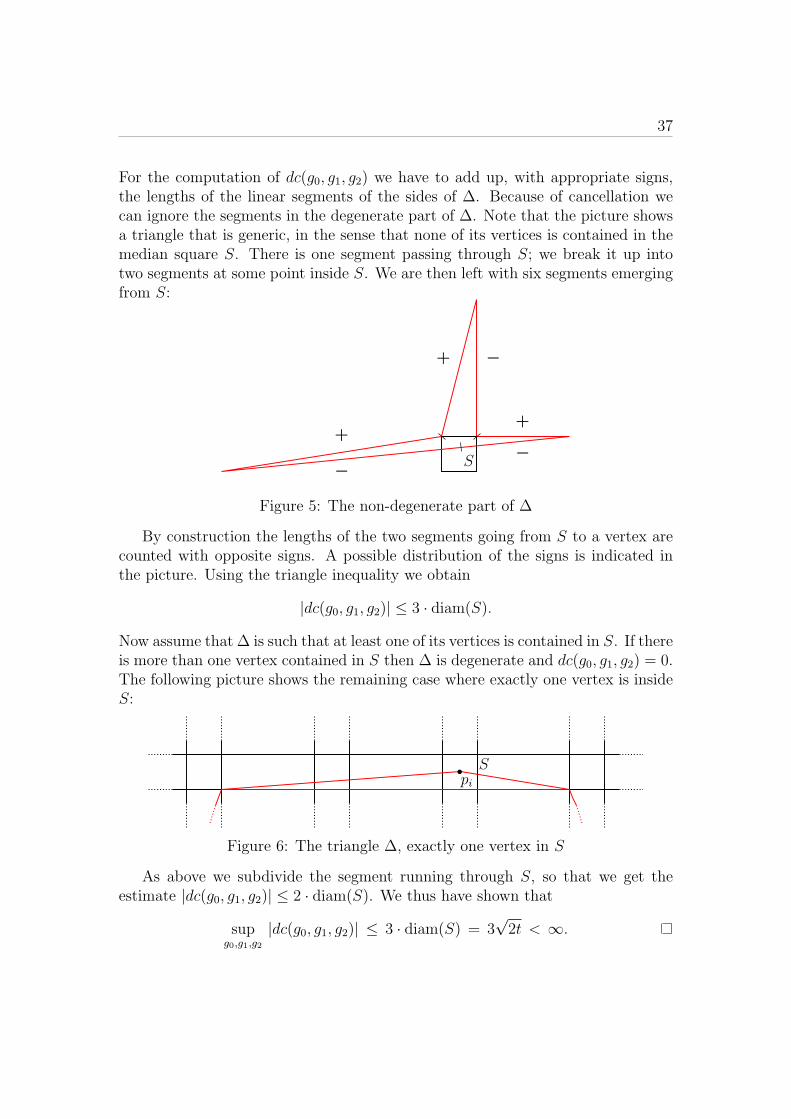
For the computation of dc(g0, g1, g2) we have to add up, with appropriate signs,the lengths of the linear segments of the sides of ∆. Because of cancellation wecan ignore the segments in the degenerate part of ∆. Note that the picture showsa triangle that is generic, in the sense that none of its vertices is contained in themedian square S. There is one segment passing through S; we break it up intotwo segments at some point inside S. We are then left with six segments emergingfrom S:
S
+
−+
−
+ −
Figure 5: The non-degenerate part of ∆
By construction the lengths of the two segments going from S to a vertex arecounted with opposite signs. A possible distribution of the signs is indicated inthe picture. Using the triangle inequality we obtain
|dc(g0, g1, g2)| ≤ 3 · diam(S).
Now assume that ∆ is such that at least one of its vertices is contained in S. If thereis more than one vertex contained in S then ∆ is degenerate and dc(g0, g1, g2) = 0.The following picture shows the remaining case where exactly one vertex is insideS:
Spi
Figure 6: The triangle ∆, exactly one vertex in S
As above we subdivide the segment running through S, so that we get theestimate |dc(g0, g1, g2)| ≤ 2 · diam(S). We thus have shown that
supg0,g1,g2
|dc(g0, g1, g2)| ≤ 3 · diam(S) = 3√2t < ∞.

38
Proposition 5.2. The quasimorphism ft,α,β is non-trivial for all parameters 0 <t < min{α, β}.
Proof. Let f be the homogenization of f = ft,α,β, where 0 < t < min{α, β}. We
show that f is not a homomorphism, which is equivalent to saying that f is non-trivial. We have f(a) = α+ t, since for n > 0 the geodesic from p to an.p consists
of a single segment of length n(α+ t). Likewise we have f(b) = β + t. In order to
compute f(ab) we consider the geodesic from p to (ab)n.p for n > 0:
p
Figure 7: The geodesic [p, (ab)n.p]
If we remove the first two and the last two segments of this geodesic we are leftwith n− 2 segments of length
√α2 + t2 and n− 2 segments of length
√β2 + t2. It
follows that f(ab) =√α2 + t2+
√β2 + t2, so that the condition f(ab) = f(a)+f(b)
is equivalent to√α2 + t2 +
√β2 + t2 = α + β + 2t.
This equation does not hold when t > 0, and hence, f is not a homomorphism inthis case and therefore f is non-trivial for t > 0.
In the remainder of this section we describe a possible generalization of ourconstruction. Let Γ = ⟨a, b⟩ free of rank two as above and let X = (X, dX) bea CAT(0) space equipped with a proper and cocompact isometric action of Γ.Choose a basepoint p ∈ X. For g = xk11 · · · xknn ∈ Γ we consider the points
qi := xixi+1 · · · xn.p, 1 ≤ i ≤ n

39
and we set qn+1 := p. We denote by qi the nearest point projection of qi onto thegeodesic [p, g.p]. We then set
f(g) =n∑
i=1
sgn(ki)dX(qi, qi+1)
to define a function f : Γ −→ R. If we chose for X a polygonal tree T asabove then the points qi are exactly the “turning points” of the geodesic and theresulting function f is the quasimorphism ft,α,β. In general, the piecewise geodesicpath along the points
p = qn+1, qn, . . . , q2, q1 = g.p
describes a quasigeodesic from p to g.p, which can be seen as a deformed version ofthe geodesic [p, g.p], and one could call the function f a “geometrically deformed”homomorphism. Unfortunately, we do not know the conditions under which fis a quasimorphism, having verified this property only in the above example. Anatural case to consider would be the universal cover a compact hyperbolic surfacewith boundary, acted upon by the fundamental group.

40
6 A common generalization of split and defor-
mation quasimorphisms
In this section we introduce a class of quasimorphisms that generalizes both con-struction that we have discussed so far.
6.1 The construction
Let Γ = A∗B. Let {f b1,b2A } ⊂ QMalt(A) be a family of alternating quasimorphisms,
one for each pair (b1, b2) ∈ B × B. Likewise let {fa1,a2B } ⊂ QMalt(B). We require
these families to satisfy the following conditions:
(i) fa1,a2B = f
a−12 ,a−1
1B and f b1,b2
A = fb−12 ,b−1
1A for all a1, a2 ∈ A and b1, b2 ∈ B.
(ii) supa1,a2∈A
∥fa1,a2B − f 1,1
B ∥∞ <∞ and supb1,b2∈B
∥f b1,b2A − f 1,1
A ∥∞ <∞
The second condition is equivalent to the boundedness of the family {f b1,b2A } as a
subset of the space (Map(A,R), ∥ · ∥∞), and likewise for the fB-family. We definea map f := {f b1,b2
A } ∗ {fa1,a2B } : Γ −→ R. For g ∈ Γ, g = a1b1 · · · anbn, set
f(g) := f 1,b1A (a1) + fa1,a2
B (b1) + f b1,b2A (a2) + . . .+ f
bn−1,bnA (an) + fan,1
B (bn).
We also write f(b1, a, b2) for fb1,b2A (a) and f(a1, b, a2) for f
a1,a2B (b). With this nota-
tion the definition of f reads
f(g) =f(1, a1, b1) + f(a1, b1, a2) + f(b1, a2, b2) + . . .
+ f(bn−1, an, bn) + f(an, bn, 1).
Proposition 6.1. If the families {f b1,b2A }, {fa1,a2
B } satisfy the above two conditionsthen the map f is an alternating quasimorphism on Γ.
We first establish some estimates involving the following quantities:
S := max{ sup ∥fa1,a2B − f 1,1
B ∥∞, sup ∥fb1,b2A − f 1,1
A ∥∞ }D := max{def f 1,1
A , def f 1,1B }
Lemma 6.2. (i) For all b1, b2, b′1, b
′2 ∈ B and all a ∈ A we have
|f(b1, a, b2)− f(b′1, a, b′2)| ≤ 2S,
and likewise with A- and B-letters exchanged.

41
(ii) For all b1, b2, b′1, b
′2, b
′′1, b
′′2 ∈ B and all a1, a2 ∈ A we have
|f(b1, a1, b2) + f(b′1, a2, b′2)− f(b′′1, a1a2, b′′2)| ≤ 3S +D,
and likewise with A- and B-letters exchanged.
Proof. (i) This is immediate from the definition of S and the triangle inequality.
(ii) By definition of S and D we have
|f(b1, a1, b2) + f(b′1, a2, b′2)− f(b′′1, a1a2, b′′2)|
≤ 3S + |f(1, a1, 1) + f(1, a2, 1)− f(1, a1a2, 1)| ≤ 3S +D.
Proof of Proposition 6.1. Let g, h ∈ Γ.
1st case: There is no cancellation in the product gh, i.e. g, h have factorizationsg = xa, h = bx′ for some x, x′ ∈ Γ, a ∈ A, b ∈ B. This means that x = x1 · · · xnends with a B-letter and x′ = x′1 · · · x′m begins with an A-letter. We have
f(gh) = f(1, x1, x2) + f(x1, x2, x3) + · · ·+ f(xn−1, xn, a)
+ f(xn, a, b) + f(a, b, x′1) + f(b, x′1, x′2) + · · ·+ f(x′m−1, x
′m, 1)
= f(g) + f(h) + f(xn, a, b)− f(xn, a, 1) + f(a, b, x′1)− f(1, b, x′1),
and hence |∂f(g, h)| ≤ 4S by Lemma 6.2.(i). Note that we get the same estimateif x = 1 (or x′ = 1), in this case the xn’s are replaced by 1 in the last line of theabove equation (or the x′1’s are replaced by 1).
2nd case: There is cancellation in gh, i.e. g, h have factorizations of the formg = xa1y, h = y−1a2x
′, where a1a2 = 1 (or likewise with B-letters instead ofA-letters). Let y have the power factorization y1 · · · yk We have
f(g) + f(h) =f(1, x1, x2) + . . .
+ f(xn−1, xn, a1) + f(xn, a1, y1) + f(a1, y1, y2)
+ f(y−12 , y−1
1 , a2) + f(y−11 , a2, x
′1) + f(a2, x
′1, x
′2)
+ · · ·+ f(x′m−1, x′m, 1)
Here we used the property f(yi−1, yi, yi+1) = −f(y−1i+1, y
−1i , y−1
i−1), due to which the

42
terms of this type cancel in the above sum. We have gh = xa1a2x′, and so
f(g) + f(h)− f(gh)= f(xn−1, xn, a1) + f(xn, a1, y1) + f(a1, y1, y2)
+ f(y−12 , y−1
1 , a2) + f(y−11 , a2, x
′1) + f(a2, x
′1, x
′2)
− f(xn−1, xn, a1a2)− f(xn, a1a2, x′1)− f(a1a2, x′1, x′2)= f(xn−1, xn, a1)− f(xn−1, xn, a1a2)
+ f(a2, x′1, x
′2)− f(a1a2, x′1, x′2)
+ f(a1, y1, y2) + f(y−12 , y−1
1 , a2)
+ f(xn, a1, y1) + f(y−11 , a2, x
′1)− f(xn, a1a2, x′1)
We can estimate each line of this sum using Lemma 6.2, it follows that
|∂f(g, h)| ≤ 2S + 2S + 2S + (3S +D) = 9S +D.
As usual we can reverse the role of the A- and B-letters in these computations.Altogether we have shown that f is a quasimorphism with def f ≤ 9S +D. Thefact that f is alternating follows from condition (i) above and the fact that westarted with families of alternating quasimorphisms.
6.2 Examples
Let fA ∈ QMalt(A), fB ∈ QMalt(B) and set f b1,b2A := fA and fa1,a2
B := fB for alla1, a2, b1, b2. In this case the quasimorphism {f b1,b2
A } ∗ {fa1,a2B } is nothing but the
split quasimorphism fA ∗ fB.A less obvious example is given by the geometric deformation quasimorphisms
ft,α,β ∈ QMalt(Γ), Γ = ⟨a⟩ ∗ ⟨b⟩ ∼= F2, defined in Section 5. Recall that such aquasimorphism f is given by
f(g) =n∑
i=1
sgn(ki)ℓ(si)
for g = xk11 xk22 · · · xknn , xi ∈ {a, b}, where si is the segment corresponding to xkii
in the geodesic [g, g.p] in the complex T . Here the length of the segment si onlydepends on the number ki and the signs of ki−1 and ki+1. This can be seen in thefollowing illustrations that show the different possible segments for bma2bn:

43
m,n > 0
m < 0, n > 0
m = 0, n > 0
m = n = 0
By symmetry of the construction the remaining possibilities for the signs of m,nyield one of the above segments. We have f = {f b1,b2
A }∗{fa1,a2B } where the families
{f b1,b2A }, {fa1,a2
B } are as follows: For k = 0 the value of f bm,bn
A (ak) = f(bm, ak, bn) isgiven by the oriented length of the geodesic segment of the geodesic [p, (bmakbn).p]corresponding to the factor ak. From the triangle inequality it follows that
|f(bm, ak, bn)− f(1, ak, 1)|
is uniformly bounded in m,n. Furthermore the construction is such that
f(bm, ak, bn) = f(b−n, ak, b−m)
44
for all m,n, k. This means that the two conditions (i) and (ii) are satisfied.
6.3 Computing the Gromov norm
Here we compute the Gromov norm for certain quasimorphisms of the type con-structed in 6.1, notably for geometric deformation quasimorphisms. In fact weverify that, under some assumptions, equality holds in Theorem 1.2 for the thequasimorphism f = {f b1,b2
A } ∗ {fa1,a2B }. We show this by adapting the proof of
Lemma 3.2.
Lemma 6.3. Let f = {f b1,b2A } ∗ {fa1,a2
B } as above. The homogenization f is given
by f(g) = f 1,1A (g) if g ∈ A, by f(g) = f 1,1
B (g) if g ∈ B, and by
f(g) =f(xn, x1, x2) + f(x1, x2, x3)
+ · · ·+ f(xn−2, xn−1, xn) + f(xn−1, xn, x1)
if g ∈ A ∪B. Here x = x1x2 · · · xn is any cyclically reduced conjugate of g.
Proof. The case g ∈ A is immediate since f(gn) = f(1, gn, 1) = f 1,1A (gn), and
likewise for g ∈ B. Let g ∈ A ∪ B and pick any cyclically reduced conjugate x ofg as in the statement. For k > 0 we compute
f(xk)
= k · [f(xn, x1, x2) + f(x1, x2, x3)
+ · · ·+ f(xn−2, xn−1, xn) + f(xn−1, xn, x1)]
+ f(1, x1, x2)− f(xn, x1, x2) + f(xn−1, xn, 1)− f(xn−1, xn, x1).
Since f(g) = f(x) the claim follows.
Let f be a quasimorphism on a group Γ and let X be a subset of Γ × Γ. Wesay that def f is realized on X if def f = sup(g,h)∈X |∂f(g, h)|. For a free productΓ = A ∗B we consider the sets SA, SB ⊂ Γ× Γ given by
SA :={(xa1y, y
−1a2x′) |a1, a2 ∈ A, a1a2 = 1, ℓ(x), ℓ(x′), ℓ(y) ≥ 2
}SB :=
{(xb1y, y
−1b2x′) |b1, b2 ∈ B, b1b2 = 1, ℓ(x), ℓ(x′), ℓ(y) ≥ 2
}Here the length ℓ(x) of x ∈ Γ is the number of power factors needed to write x as areduced product of A- and B-letters (e.g. ℓ(ab−2a−1b6) = 4). We let S := SA∪SB.
Lemma 6.4. Let f = {f b1,b2A } ∗ {fa1,a2
B } as above. If def f is realized on S then
def f ≥ 2 def f .

45
Proof. Let (g, h) ∈ S. We may assume that (g, h) ∈ SA, i.e. g = xa1y, h = y−1a2x′
with ℓ(x), ℓ(x′), ℓ(y) ≥ 2 and a1a2 = 1. We want to find g, h ∈ Γ such that
∂f(g, h) = 2 ·∂f(g, h). We may assume that there is no cancellation in the productx′x, since we may replace x′ by x′a or x′b without changing the quantity ∂f(g, h).(See case 2 above). Choose t ∈ Γ non-trivial such that there is no cancellation inyty. Define
g := y−1a2x′xa1yt
h := t−1y−1a2x′xa1y.
We have
f(g) + f(h) = 2[f(y−12 , y−1
1 , a2) + f(y−11 , a2, x
′1) + f(a2, x
′1, x
′2)
+ · · ·+ f(xn−1, xn, a1) + f(xn, a1, y1) + f(a1, y1, y2)]
Note that all the terms involving factors of t cancel in this sum. A cyclicallyreduced conjugate of gh is given by a1a2x
′xa1a2x′x = (a1a2x
′x)2. We compute
f(gh) = 2 f(a1a2x′x)
= 2[f(xn, a1a2, x′1) + f(a1a2, x
′1, x
′2) + · · ·+ f(xn−1, xn, a1a2)]
Using the computation in the proof of Proposition 6.1, 2nd case, we see that∂f(g, h) = 2 · ∂f(g, h). The claim follows.
Theorem 6.5. Let f = {f b1,b2A } ∗ {fa1,a2
B } as above, with associated cohomologyclass ωf . If def f is realized on S then
∥ωf∥ = def f = 12def f
In particular, equality holds in Theorem 1.2 for the quasimorphism f .
Proof. By Theorem 1.2 and Lemma 6.4 we have
def f ≥ ∥ωf∥ ≥ 12def f ≥ def f,
the claim follows.
It is easy to see that for a split quasimorphism f the defect is realized on S, soTheorem 6.5 applies in this case (and is therefore a generalization of Theorem 3.3).
For the rest of this section we consider geometric deformation quasimorphismsft,α,β on Γ = Z ∗ Z. Again, we denote by S ⊂ Γ× Γ the subset defined above.
Lemma 6.6. For all α, β > 0 and 0 < t < max{α, β} the defect of ft,α,β is realizedon S.

46
Proof. We assume, without loss of generality, that α ≥ β. Using elementarygeometry, it is not hard to see that the defect of the homogenous quasicocycle cassociated to ft,α,β is realized by a triangle with the following core:
One computes
def ft,α,β = 2√β2 + t2 − 2β − t+
√α2 + t2 − α.
This defect is realized for example by (g, h) = (babab, b−1a−1ba−1b−1), a pair whichbelongs to the set S.
The following statement is now immediate:
Theorem 6.7. For all geometric deformation quasimorphisms ft,α,β with α, β > 0and 0 < t < max{α, β} equality holds in Theorem 1.2.
In case the defect of a quasimorphism f = {f b1,b2A } ∗ {fa1,a2
B } is not realized onS we are not able to compute the Gromov norm of ωf . The problem is that for apair (g, h) which realizes the defect, terms of the form f(1, a, b) or f(b, a, 1) could
occur in ∂f(g, h). The homogenization f however ignores these terms, so that our
argument showing that def f ≥ 2 · def f does not apply.
47
7 Defect spaces
7.1 Definition and first properties
Let Γ be a group. The defect space of Γ, denoted by D(Γ), is the space of functionsf : Γ −→ R that are bounded and alternating (i.e. f(g−1) = −f(g) for all g ∈ Γ),equipped with the norm
∥f∥def = def f = supg,h∈Γ
|∂f(g, h)|,
where ∂f(g, h) = f(g) + f(h)− f(gh). This is indeed a norm: If ∥f∥def = 0 thenf is a bounded homomorphism into R and hence equal to zero. Homogenity andthe triangle inequality are immediate. Thus we have two norms on the space of(alternating) bounded functions on Γ, the ℓ∞-norm and the defect norm. Thesenorms turn out to be equivalent. This follows essentially from the following state-ment, in which ord(g) stands for the (possibly infinite) order of a group elementg ∈ Γ.
Proposition 7.1. For f ∈ D(Γ) and g ∈ Γ, g = e, we have the estimate
|f(g)| ≤(1− 2
ord(g)
)∥f∥def .
Proof. We may assume that ∥f∥def = 1. For n ≥ 1 we have the estimate
|f(gn)− nf(g)| ≤ n− 1,
which follows from
|f(gn)− nf(g)| =
∣∣∣∣∣n−1∑i=1
f(gi+1)− f(gi)− f(g)
∣∣∣∣∣ ≤ (n− 1)∥f∥def .
If g has finite even order 2k then f(gk) = 0, as f is alternating, so the aboveestimate implies k|f(g)| ≤ k− 1 which means that |f(g)| ≤ 1− 1
k= 1− 2
ord(g). If g
has order 2k+1 then we have f(gk)+ f(gk+1) = 0, so summation of the estimates
|f(gk)− kf(g)| ≤ k − 1
|f(gk+1)− (k + 1)f(g)| ≤ k
yields (2k + 1)|f(g)| ≤ 2k − 1, so |f(g)| ≤ 1 − 22k+1
= 1 − 2ord(g)
. Finally, if g
has infinite order then letting n tend to infinity in |f(gn)
n− f(g)| ≤ 1 − 1
nyields
|f(g)| ≤ 1.

48
Corollary 7.2. The defect norm is equivalent to the supremum norm ∥ ·∥∞, moreprecisely, for f ∈ D(Γ) we have
∥f∥∞ ≤ ∥f∥def ≤ 3∥f∥∞.
The space D(Γ) is therefore a Banach space. It is infinite dimensional if and onlyif Γ has infinitely many elements of order different from 2, and in this case it isnon-separable.
Proof. The lower bound is a consequence of the proposition, the upper bound isimmediate from the definition of the defect norm.
The following function f ∈ D(Z) shows that the supremum in the definition ofthe defect norm need not be attained:
f(k) =
0, k even
1− 1/k, k > 0 odd1/k − 1, k < 0 odd.
Here we have ∥f∥def = 2 but |∂f(k, l)| < 2 for all k, l ∈ Z.
Proposition 7.3. An epimorphism π : Γ −→ Q induces an isometric embeddingπ∗ : D(Q) ↪−→ D(Γ), f 7→ f ◦ π.
Proof. By surjectivity of π we have
∥π∗f∥def = supg,h∈Γ
|∂f(π(g), π(h))| = supg,h∈Q
|∂f(g, h)| = ∥f∥def .
Proposition 7.4. For a monomorphism i : H −→ Γ, the map
si : D(H) −→ D(Γ), si(f)(g) =
{f(h), g = i(h)0, g ∈ i(H)
is an isometric embedding.
Proof. We write F := si(f) and we identify H with its image i(H). Let g, h ∈ Γ.Of the three elements g, h, gh either none, one or all three belong to H. In the firstcase we have ∂F (g, h) = 0, in the second case we have |∂F (g, h)| ≤ ∥f∥∞ ≤ ∥f∥def(by Proposition 7.1 and Corollary 7.2) and in the last case we have |∂F (g, h)| =|∂f(g, h)| ≤ ∥f∥def . So we have ∥F∥def ≤ ∥f∥def . As i is injective we also have thereverse inequality, i.e. ∥F∥def = ∥f∥def .

49
In case of a normal subgroup the last statement can be improved. Consider ashort exact sequence
1 // Ni // Γ π // Q // 1. (2)
We have the following maps between the defect spaces
D(Q) π∗// D(Γ)
i∗ // D(N),si
oo
where i∗ ◦π∗ = 0 and si is a section of i∗. This means that the embeddings π∗ andsi are complementary. More precisely, we have
Proposition 7.5. For the short exact sequence (2) we have an isometric embed-ding
j : D(N)⊕∞ D(Q) ↪−→ D(Γ)which is given by j = si + π∗, and, more explicitly, by
j(f, f ′)(g) =
{f(n), g = i(n)
f ′(π(g)), g ∈ i(N).
Here the notation ⊕∞ stands for the max-norm on the direct sum.
Proof. For (f, f ′) ∈ D(N)⊕D(Q) we write F := j(f, f ′). We identify N with itsimage i(N). We first note that for g ∈ N ⊂ Γ we have π∗(f ′)(g) = f ′(eN) = 0,so F (g) = f(g), which proves the explicit formula for j. Now let g, h ∈ Γ. Ifnone of g, h, gh is contained in N then |∂F (g, h)| = |∂f ′(π(g), π(h))| ≤ ∥f ′∥def . Ifg ∈ N, h ∈ N then π(h) = π(gh), so
|∂F (g, h)| = |f(g) + f ′(π(h))− f ′(π(gh))| = |f(g)| ≤ ∥f∥∞ ≤ ∥f∥def ,
by Proposition 7.1 and Corollary 7.2. Because of the identities
|∂F (g, h)| = |∂F (h−1, g−1)| = |∂F (g−1, gh)|
the same holds true whenever exactly one of g, h, gh is contained in N . If allthree elements are in N then |∂F (g, h)| = |∂f(g, h)| ≤ ∥f∥def . It follows that∥F∥def ≤ max{∥f∥def , ∥f ′∥def}, and the reverse inequality holds since the maps siand π∗ are isometric.
Lemma 7.6. For i = 1, 2 consider short exact sequences
1 // Ni// Γ // Qi
// 1 (3)
with Qi = {e}. We identify Ni with its image in Γ. Assume that Γ = N1N2. LetVi be the image of the embedding ji : D(Ni)⊕∞ D(Qi) ↪−→ D(Γ). We have
V1 ∩ V2 = {f ∈ D(Γ) | supp(f) ⊂ N1 ∩N2}.

50
Proof. Let f ∈ V1∩V2 and let g ∈ Γ \N1 and h ∈ Γ \N2. Since N1N2 = Γ we have
gN1 ∩ hN2 = ∅gN1 ∩ h−1N2 = ∅
By construction f is constant on non-trivial cosets, so we have f(g) = f(h) but alsof(g) = f(h−1) = −f(h) and therefore f(g) = f(h) = 0. This proves the “⊆” partof the claim. The reverse containment is immediate, for f with supp(f) ⊂ N1∩N2
we can choose fNi= f |Ni
and fQi= 0 to obtain f = ji(fNi
, fQi) for i = 1, 2.
When applied to direct products this lemma yields the following statement:
Proposition 7.7. For a product Γ = Γ1 × Γ2 the induced isometric embeddings
j1, j2 : D(Γ1)⊕∞ D(Γ2) ↪−→ D(Γ)
are given by
j1(f1, f2)(g1, g2) =
{f1(g1), g2 = ef2(g2), g2 = e,
j2(f1, f2)(g1, g2) =
{f1(g1), g1 = ef2(g2), g1 = e.
and the images of these embeddings intersect trivially in D(Γ).
7.2 Existence of extremal points
Recall that a point of a convex subset C of a real vector space is called extremal ifit is not a proper convex combination of two points in C. The theorem of Krein-Milman (see for example [58], Theorem 2.3.4) asserts that in a locally convex vectorspace, any compact convex set is the closed convex hull of its extremal points (andin particular that the set has extremal points). This statement applies to theclosed unit ball in the isometric dual X∗ of a Banach space X, which by thetheorem of Banach–Alaoglou (see for example [48], Theorem 3.15) is compact inthe weak*-topology. In this subsection we discuss extremal points in the spacesof our interest. For the space ℓ∞alt(Γ) there is not much to say: This space is thedual of ℓ1alt(Γ) and indeed the set of extremal points in the closed unit ball is easilyidentified as the set
{f ∈ ℓ∞alt(Γ) | |f(g)| = 1 if g2 = e}
Note that the only information about Γ that is encoded in the space ℓ∞alt(Γ) is thecardinal
dim ℓ∞alt(Γ) = |{g ∈ Γ | g2 = e}|.

51
It turns out that the set of extremal points in the equivalent space D(Γ) has amuch richer structure that reflects properties of the group Γ.
In the following we denote by
B(Γ) := {f ∈ D(Γ) | ∥f∥def ≤ 1}
the closed unit ball in D(Γ) and by E(Γ) the set of extremal points of B(Γ). Incase D(Γ) = {0}, i.e. when Γ is a 2-torsion group or trivial, we use the conventionE(Γ) := {0}. It is not a priori clear that E(Γ) is non-empty for all groups Γ. Thisfacts follows from
Theorem 7.8. For a countable discrete group Γ, there exists a Banach space whoseisometric dual is D(Γ). More precisely there is an equivalent norm ∥ · ∥′ on thespace (ℓ1alt(Γ), ∥ · ∥ℓ1) such that the isometric dual of (ℓ1alt(Γ), ∥ · ∥′) is isomorphicto D(Γ).
This is a consequence of the following standard lemma from the renormingtheory of Banach spaces:
Lemma 7.9 ([24], Lemma 8.8). Let (X, ∥ · ∥) be a Banach space, and let ∥ · ∥′ bean equivalent norm on the isometric dual X∗. Then ∥ · ∥′ is a dual norm to someequivalent norm on X if and only if ∥ · ∥′ is weak*-lower semicontinuous.
Proof of Theorem 7.8. For g ∈ G let αg ∈ ℓ1alt(G) be given by αg = δg − δg−1 . Forg, h ∈ G we define βg,h := αg + αh − αgh. Now assume that the sequence {fn} ⊂D(G) converges to f ∈ D(G) in the weak*-topology. Since ⟨f, βg,h⟩ = 2 · ∂f(g, h)we deduce that for all g, h ∈ G we have the convergence ∂fn(g, h)→ ∂f(g, h). Forε > 0 pick g0, h0 ∈ G such that ∥f∥def − ε < |∂f(g0, h0)|. Now in the inequality|∂fn(g0, h0)| ≤ ∥fn∥def pass to the limit inferior to obtain
∥f∥def − ε < |∂f(g0, h0)| ≤ lim infn→∞
∥fn∥def ,
so ∥f∥def ≤ lim infn→∞ ∥fn∥def . This means that ∥ · ∥def is weak*-lower semicon-tinuous. Now the statement follows from Lemma 7.9.
Corollary 7.10. The unit ball B(Γ) is the closed convex hull of its set of extremalpoints E(Γ). In particular we have E(Γ) = ∅ for every group Γ.
In order to study the geometry of the Banach space (ℓ1alt(Γ), ∥ · ∥′) it would beuseful if one could express the norm ∥ · ∥′ of Theorem 7.8 explicitly, however, wehave not succeeded in finding such a description.
We now collect a number of useful facts for later use.
Lemma 7.11. If f ∈ B(Γ) satisfies |∂f(g, g)| = 1 for all g ∈ Γ with g2 = e, thenf ∈ E(Γ).
52
Proof. Assume f ± ε ∈ B(Γ) for some non-zero ε ∈ D(Γ). We show that for allg ∈ Γ the relation ε(g2) = 2ε(g) holds. This implies ε(g2
n) = 2nε(g), hence ε = 0
by boundedness. So let g ∈ Γ. If g2 = e then ε(g2) = 0 = 2ε(g). For g2 = e wemay assume that ∂f(g, g) = 1, otherwise replace g by g−1. From the inequality
1 ≥ ∂(f ± ε)(g, g) = 1± ∂ε(g, g)
it follows that ∂ε(g, g) = 0, i.e. ε(g2) = 2ε(g).
For the next statement we consider the subset
E∗(Γ) := {f ∈ B(Γ) | |∂f(g, h)| = 1 whenever g, h, gh = e} (4)
As the notation suggests, this set consists of extremal points. These points havethe additional property of being stable under restriction to subgroups:
Proposition 7.12. (i) The set E∗(Γ) is contained in E(Γ).
(ii) The set E∗(Γ) is a discrete subset of D(Γ).
(iii) If f ∈ E∗(Γ) then f |H ∈ E∗(H) for every subgroup H < Γ.
Proof. The first statement follows at once from Lemma 7.11. In order to provethe second statement let f, f ′ ∈ E∗(Γ), f = f ′. We have ∂f = ∂f ′, otherwise∂(f − f ′) = 0 and hence f = f ′ by boundedness. Hence there exist g, h ∈ Γ with∂f(g, h) = ∂f ′(g, h), which means that ∂f(g, h) = 1 and ∂f ′(g, h) = −1 or viceversa, i.e.
∥f − f ′∥def ≥ |∂(f − f ′)(g, h)| = 2.
The last statement is obvious from the definition of E∗.Proposition 7.13. If f ∈ E(Γ) then for all g ∈ Γ with g2 = e we have
suph∈Γ|∂f(g, h)| = sup
h∈Γ|∂f(h, g)| = 1.
Proof. Assume that for some s ∈ Γ, s2 = e, and some ε > 0 we have suph∈Γ |∂f(s, h)| =1− ε. Let αs = δs − δs−1 ∈ D(Γ). Since s2 = e we have αs = 0. We show that thefunctions
f± := f ± ε/4 · αs
are contained in B(Γ), so that f is not extremal. Let g, h ∈ Γ. If none of g, h, ghis equal to s±1 then |∂f±(g, h)| = |∂f(g, h)| ≤ 1. If g = s then
|∂f±(g, h)| ≤ |∂f(g, h)|+ 14ε|∂αs(g, h)| ≤ 1− ε+ 3
4ε = 1− 1
4ε < 1.
Because of the identities
|∂f±(g, h)| = |∂f±(g−1, gh)| = |∂f±(h, h−1g−1)| = |∂f±(gh, h−1)|
the same estimate holds if any of g, h, gh is equal to s±1.

53
7.3 Extremal points for finite groups
Let Γ be a finite group. In the space ℓ∞alt(Γ) the closed unit ball
{f ∈ ℓ∞alt(Γ) | |f(g)| ≤ 1 for all g ∈ Γ}
can be seen as the unit cube of this space. For the equivalent defect space we have
Proposition 7.14. For a finite group Γ the closed unit ball B(Γ) ⊂ D(Γ) is apolytope (i.e. a bounded intersection of finitely many closed halfspaces)
Proof. For f ∈ D(Γ) the condition ∥f∥def ≤ 1 means that all of the finitely manylinear inequalities
f(g) + f(h)− f(gh) ≤ 1, g, h ∈ Γ
f(g) + f(h)− f(gh) ≥ −1, g, h ∈ Γ
are satisfied simultaneously. Now each of these inequalities has as its set of solu-tions a closed halfspace in D(Γ).
The extremal points E(Γ) for a finite group Γ are therefore precisely the verticesof the polytope B(Γ). This polytope depends on the group and not merely on thedimension of the space. This is illustrated by the following pictures, which showthe unit balls in the 2-dimensional defect spaces D(Z/5), D(Z/6) and D(Z/2×Z/4)(in this order):
Here the shaded regions are the defect-norm unit balls. Furthermore, as an illus-tration of the inequalities of Corollary 7.2, we see the ℓ∞-spheres of radius 1/3 and1 contained in, respectively containing these unit balls (the frames of the picturesare the spheres of radius 1).
7.4 Left orders and extremal points with maximal sup-norm
Here we identify the subset
E1(Γ) := {f ∈ E(Γ) | f(Γ \ {e}) = {±1} }

54
of E(Γ). Proposition 7.1 implies that E1(Γ) = ∅ whenever Γ has torsion. Indeed,the proposition says that for any f ∈ E(Γ) and g ∈ Γ of order 1 < n <∞ we have|f(g)| ≤ 1− 2
n, hence f ∈ E1(Γ). It turns out that the obstruction to the existence
of points in E1(Γ) is not just torsion but in fact the lack of a left-order on Γ. Wesay that a relation ≤ on Γ is a left-order if it is a total left-invariant order. Thismeans that for all g, g′, g′′ ∈ Γ we have
(i) g ≤ g′ and g′ ≤ g =⇒ g = g′
(ii) g ≤ g′ and g′ ≤ g′′ =⇒ g ≤ g′′
(iii) One of g ≤ g′ and g′ ≤ g holds.
(iv) g ≤ g′ =⇒ hg ≤ hg′ for all h ∈ Γ
As usual we write g < h if we have g ≤ h and g = h. If a relation satisfies theabove conditions except perhaps the third one then we call it a partial left-order.We equip the set of partial left-orders PLO(Γ) with the topology that is definedby basis sets of the form
Ug1,g2,...,gn := {≤ ∈ PLO(Γ) | g1 < g2 < · · · < gn}.
The induced topology on the subspace of left-orders LO(Γ) was introduced bySikora in [50]. The following are fundamental results concerning this space:
Theorem 7.15 ([50], Theorem 1.4). For every group Γ the space LO(Γ) is totallydisconnected and compact.
Theorem 7.16 ([37], Theorem 1.3). For every group Γ the space LO(Γ) is eitherfinite or uncountably infinite.
Let now ≤ be a given partial left-order on a group Γ. Since we have g > e⇐⇒g−1 < e we obtain a map f≤ ∈ D(Γ) by setting
f≤(g) :=
1, g > e−1, g < e0, else.
We writeBint(Γ) := {f ∈ B(Γ) | f(Γ) ⊂ {0,±1}},
this is the set of integral-valued functions that are contained in the unit ball ofD(Γ).
Lemma 7.17. For every ≤ ∈ PLO(Γ) we have f≤ ∈ Bint(Γ).

55
Proof. We have to show that ∥f≤∥def ≤ 1. For g, h ∈ Γ write D = |∂f≤(g, h)|. Byleft-invariance it follows that either none, one or all three of g, h, gh are comparableto e. In the first case we have D = 0. In the second case we have D = 1. Inthe third case we have either f≤(g) = f≤(gh) and hence D = |f≤(h)| = 1, orwe have f≤(g) = −f≤(gh) and we may assume, without loss of generality, g > eand gh < e. By left-invariance this means h < g−1 < e, hence f≤(h) = −1 andD = 1.
Now let f ∈ Bint(Γ). We define a relation ≤f on Γ by
g ≤f h :⇐⇒ f(g−1h) = 1
for g = h, and g ≤f g for all g ∈ Γ.
Lemma 7.18. For every f ∈ Bint(Γ) we have ≤f ∈ PLO(Γ).
Proof. We show first that the relation is transitive. Let g ≤f g′ ≤f g′′, i.e.f(g−1g′) = f(g′−1g′′) = 1. We have
∂f(g−1g′, g′−1g′′) = 2− f(g−1g′′)
and hence f(g−1g′′) = 1, so g ≤f g′′. Now assume that g ≤f g′ and g′ ≤f g.If g = g′ this means that f(g−1g′) = f(g′−1g) = 1 which is impossible as f isalternating, so g = g′. The fact that ≤f is left-invariant is obvious.
Lemma 7.19. The assignments f 7→≤f and ≤ 7→ f≤ are mutually inverse.
Proof. Let f ′ ∈ Bint(Γ) and let g ∈ Γ. We have
f≤f ′(g) = 1⇐⇒ g >f ′ e⇐⇒ f ′(g) = 1.
Likewise we have f≤f ′(g) = −1 ⇐⇒ f ′(g) = −1, and therefore f≤f ′
= f ′. On theother hand, for ≼ ∈ PLO(Γ) and g, h ∈ Γ we have
g <f≼ h⇐⇒ f≼(g−1h) = 1⇐⇒ e ≺ g−1h⇐⇒ g ≺ h
and hence ≤f≼ = ≼.
Lemma 7.20. The bijection Bint(Γ) −→ PLO(Γ) restricts to a bijection E1(Γ) −→LO(Γ).
Proof. Let f ∈ E1(Γ). We have to show that ≤f is a total order. Let g, h ∈ Γ. Ifg = h we have g ≤f h. If g = h then either f(g−1h) = 1 or f(h−1g) = −f(g−1h) =1, hence g ≤f h or h ≤f g

56
Theorem 7.21. If we endow the set Bint(Γ) with the topology induced from theweak*-topology on D(Γ) then the mutually inverse maps
Bint(Γ) −→ PLO(Γ), f 7→ ≤f
PLO(Γ) −→ Bint(Γ), ≤ 7→ f≤
are homeomorphisms.
By Lemma 7.20 we get
Corollary 7.22. If we endow the set E1(Γ) with the topology induced from theweak*-topology on D(Γ) then the mutually inverse maps
E1(Γ) −→ LO(Γ), f 7→ ≤f
LO(Γ) −→ E1(Γ), ≤ 7→ f≤
are homeomorphisms.
Proof of Theorem 7.21. A subbasis for the topology of the space PLO(Γ) is givenby the sets
Ug = {≤ ∈ PLO(Γ) | e < g}, g ∈ Γ
(see [37], p.1). Denote the first map in the theorem by Φ. We show that forall g ∈ Γ the preimage Φ−1(Ug) is open in Bint(Γ), which means that the map iscontinuous. We have
Φ−1(Ug) = {f ∈ Bint(Γ) | e <f g} = {f ∈ Bint(Γ) | f(g) = 1}.
Let {fn} be a sequence contained in the complement
W := Bint(Γ) \Φ−1(Ug) = {f ∈ Bint(Γ) | f(g) ∈ {0,−1}},
that weak*-converges to f ∈ Bint(Γ). By Theorem 7.8 this means that for allα ∈ ℓ1alt(Γ) we have ⟨α, fn⟩ −→ ⟨α, f⟩. For αg := δg − δg−1 we have
⟨αg, fn⟩ = fn(g)− fn(g−1) ∈ {0,−2}
for all n, hence ⟨αg, f⟩ ∈ {0,−2} which means that f(g) ∈ {0,−1}, i.e. f ∈ W .Therefore W is weak*-closed, which establishes the claim.We show next that Bint(Γ) is weak*-compact. For this purpose it is sufficient toshow that it is a closed subset of the unit ball B(Γ) which is weak*-compact bythe theorem of Banach–Alaoglou. For a sequence {fn} in Bint(Γ) with weak*-limitf we have, as above, ⟨αg, fn⟩ = 2fn(g) ∈ {0,±2}. Hence ⟨αg, f⟩ ∈ {0,±2}, whichmeans that f(g) ∈ {0,±1}. It follows that f is contained in the set Bint(Γ).Now the space Bint(Γ) is weak*-compact and the space PLO(Γ) is Hausdorff ([50],Proposition 1.3), so the continuous bijection Φ : Bint(Γ) −→ PLO(Γ) is in fact ahomeomorphism.
57
Together with Theorem 7.16 we obtain
Corollary 7.23. The set E1(Γ) is either finite or uncountably infinite.
Question. For which ≤ ∈ PLO(Γ) is f≤ ∈ E(Γ)? In other words: What charac-terizes an extremal partial left-order?
Below, after Theorem 7.25, we will see examples of partial, non-total ordersthat are extremal.
7.5 Extremal points from quotients
In 7.1 we showed that for a quotient Q = Γ/N the space D(Q)⊕∞ D(N) embedsisometrically into D(Γ). The following result states that this embedding preservesextremal points:
Theorem 7.24. For a short exact sequence
1 // N // Γ // Q // 1
in which the group Q is 2-torsion free, the induced embedding j : D(N) ⊕∞D(Q) ↪−→ D(Γ) maps extremal points to extremal points. That is, we have anembedding
E(N)× E(Q) ↪−→ E(Γ).
Proof. Let fN ∈ E(N), fQ ∈ E(Q), and let F = j(fN , fQ). We have ∥F∥def = 1.Assume that for some E ∈ D(Γ) we have F ± E ∈ B(Γ). We have to show thatE = 0. Since F |N = fN and fN is extremal, we have E|N = 0. In order to showthat E vanishes altogether, it is sufficient to show that E descends to the quotientQ, i.e. that E = e ◦ π for some e ∈ D(Q). This is because fQ is extremal. So wewant to prove that E(g) = E(gn) for any given g ∈ Γ, n ∈ N . If g ∈ N we haveE(g) = E(gn) = 0. Let now g ∈ N . Since Q is 2-torsion free, we have π(g)2 = e.By Proposition 7.13, for each 1 > ε > 0 there exists h ∈ Γ such that
|∂F (g, h)| = |∂fQ(π(g), π(h))| > 1− ε.
Since π(n) = e this implies
|∂F (gnk, h)| = |∂F (gnk−1, nh)| > 1− ε
for k ≥ 1. Therefore
|∂E(gnk, h)| < ε, |∂E(gnk−1, nh)| < ε.

58
Through the triangle inequality these estimates combine to
|E(gnk)− E(gnk−1) + E(h)− E(nh)| < 2ε, (5)
from which we deduce
|E(gnk)− E(g) + k(E(h)− E(nh))| < 2kε
by telescopic summation. We divide both sides by k and let k tend to infinity.Since E is a bounded function we get
|E(h)− E(nh)| < 2ε.
Combining this estimate with the estimate (5) for k = 1 we obtain
|E(gn)− E(g)| < 4ε.
It follows that E(gn) = E(n).
If we drop the assumption that Q be 2-torsion free the statement of the theoremis false in general. This can easily be seen in an example like Z/6 −→ Z/2.However, we can still produce extremal points for Γ if we start with suitableextremal points for N and Q, as the following statement shows. Recall that wedefined the set E∗(Γ) in equation (4) above.
Theorem 7.25. For a short exact sequence
1 // N // Γ // Q // 1.
the induced embedding j : D(N)⊕∞ D(Q) ↪−→ D(Γ) restricts to embeddings
E1(N)× E∗(Q) ↪−→ E∗(Γ)
andE1(N)× E1(Q) ↪−→ E1(Γ).
Proof. Let fN ∈ E1(N), fQ ∈ E∗(Q) and F = j(fN , fQ). Let g, h ∈ Γ such thatg, h, gh = e. If none of g, h, gh is contained in N then π(g), π(h), π(gh) = e so
|∂F (g, h)| = |∂fQ(π(g), π(h))| = 1.
Assume that exactly one of g, h, gh is contained in N . Because of the identities atthe end of the proof of Proposition 7.13 we may assume that g ∈ N , h, gh ∈ N .We have
|∂F (g, h)| = |fN(g) + fQ(π(h))− fQ(π(gh))| = |fN(g)| = 1.

59
If all three of g, h, gh are contained in N then
|∂F (g, h)| = |fN(g, h)| = 1
since fN ∈ E1(N) ⊂ E∗(N). By definition of E∗ we have F ∈ E∗(Γ). If westart with fN ∈ E1(N), fQ ∈ E1(Q) then F (Γ \ {e}) = {±1} by construction, soF ∈ E1(Γ).
Theorem 7.25 can be used to produce extremal points that have values in{0,±1} but are not contained in E1. The quotient Z −→ Z/2 for example yieldsthe extremal point f ∈ E∗(Z) given by
f(k) =
0, k = 0 or k odd1, k > 0 even−1, k < 0 even.
Note that the existence of the second embedding in the theorem reflects the factthat the class of left-orderable groups is closed under extensions.
The following statement gives a condition under which the respective extremalpoints induced from two different quotients of a group Γ are disjoint.
Proposition 7.26. For i = 1, 2 let
1 // Ni// Γ // Qi
// 1
be a short exact sequence with a 2-torsion free non-trivial group Qi. Write Si forthe image of the induced embedding ji : E(Ni) × E(Qi) ↪−→ E(Γ). If N1N2 = Γthen S1 ∩ S2 = ∅.
Proof. By Lemma 7.6 any f ∈ S1 ∩ S2 is of the form f = j1(fN1 , 0), but 0 is notcontained in E(Q1).
This statement says, for example, that the points in E(Z) obtained from quo-tients by pZ, p prime, are all distinct.
7.6 Extremal points from infinite chains of normal sub-groups
If we have a finite descending chain of normal subgroups
Γ = N0 > N1 > · · · > Nk
with 2-torsion free quotients Γ/Ni then iterated application of Theorem 7.24 yieldsan embedding
E(N0/N1)× E(N1/N2)× · · · × E(Nk−1/Nk)× E(Nk) ↪−→ E(Γ)

60
In this subsection we generalize this fact to the situation of suitable infinite chains.Let
Γ = N0 > N1 > . . .
be a descending chain of normal subgroups of Γ such that Ni = Ni+1 and suchthat
∩∞i=0Ni = {e}. Given a sequence
(fi)i = (fi)∞i=1 ∈
∞∏i=1
B(Ni−1/Ni)
we define the map f ∈ D(Γ) by f(g) = fi(gNi+1), where i is the unique indexfor which g ∈ Ni and g ∈ Ni+1. For the following statement we equip the aboveproduct of unit balls with the norm ∥(fi)i∥ := supi ∥fi∥def .
Proposition 7.27. The assignment (fi)i 7→ f describes an isometric embedding
J :∞∏i=0
B(Ni/Ni+1) ↪−→ B(Γ).
Proof. Let (fi)i be a given sequence and f = J((fi)i). We may assume that∥(fi)i∥ = 1. We first show that ∥f∥ ≤ 1. Let g, h ∈ Γ. If one of g, h, gh is trivialthen ∂f(g, h) = 0, since f is alternating. Otherwise, there exists an index i suchthat g, h, gh ∈ Ni+1. From Proposition 7.5 we obtain an isometric embedding
I : B(N0/N1)× B(N1/N2)× · · · × B(Ni/Ni+1)× B(Ni+1) ↪−→ B(Γ).
Now set α := I(f0, f1, . . . , fi, 0). By construction, we have f(g) = α(g), f(h) =α(h), f(gh) = α(gh), so that |∂f(g, h)| = |∂α(g, h)| ≤ 1. Therefore we have ∥f∥ ≤1. To prove the reverse inequality, let i be a given index and let g, h ∈ Ni \Ni+1
such that gh ∈ Ni \Ni+1. We have ∂f(g, h) = ∂fi(gNi+1, hNi+1). It follows that∥f∥ ≥ ∥fi∥def , and hence ∥f∥ ≥ supi ∥fi∥def = ∥(fi)i∥ = 1.
For a group Γ with a descending chain of normal subgroups as above, we nowconsider the inverse limit
Γ := lim←−i
Γ/Ni.
We write Ki for the kernel of the natural projection pi : Γ −→ Γ/Ni. We have thedescending chain of normal subgroups
Γ = K0 > K1 > . . . .

61
The projection pi+1 restricts to a map Ki −→ Ni/Ni+1, which induces naturalisomorphisms Ki/Ki+1
∼= Ni/Ni+1. By Proposition 7.27 we have an isometricembedding
J :∞∏i=0
B(Ni/Ni+1) ↪−→ B(Γ).
By construction, the embeddings J and J are compatible with the restriction mapr : B(Γ) −→ B(Γ), so that J = r ◦ J . The following result asserts that theseembeddings map extremal points to extremal points.
Theorem 7.28. Let Γ be a group. For an infinite descending chain of normalsubgroups
Γ = N0 > N1 > . . .
with trivial intersection and 2-torsion free quotients Γ/Ni, the associated embeddingJ restricts to an embedding
∞∏i=0
E(Ni/Ni+1) ↪−→ E(Γ).
Moreover, the restriction of J yields an embedding∞∏i=0
E(Ni/Ni+1) ↪−→ E(Γ)
and these two embeddings are compatible with the restriction map D(Γ) −→ D(Γ).Proof. We only need to prove the first statement, as the second one follows fromthe observations made before the theorem. Let (fi)i = (fi)
∞i=0 ∈
∏∞i=0 E(Ni/Ni+1)
and let F = J((fi)i). Assume that there exists E ∈ D(Γ) such that F ±E ∈ B(Γ).We have to show that E = 0. For this purpose we consider the embedding
J :∞∏i=1
B(Ni/Ni+1) ↪−→ B(N1),
which is obtained by shifting the index by 1, and the embedding
j : B(Γ/N1)⊕∞ B(N1) ↪−→ B(Γ)
from Proposition 7.5. This allows us to write the map F as F = j( f0, J( (fi)∞i=1 ) ).
By the same argument as in the proof of Theorem 7.24 the map E descends toa map on the quotient Γ/N1; more precisely, we have E(gn) = E(g) for g ∈ N1
and n ∈ N1. Since f0 is extremal, this means that E vanishes on Γ \N1. If Ealso vanishes on N1 we are done. If not, we iterate the argument to obtain thatE vanishes on N1 \N2, N2 \N3, etc. Since the intersection of the Ni is trivial, itfollows that E = 0.

62
Corollary 7.29. If the countably infinite group Γ is residually finite 2-torsion free,then its set of extremal points E(Γ) contains uncountably many rational-valuedfunctions.
Proof. Let g1, g2, . . . be an enumeration of the non-trivial elements of Γ. By as-sumption, we can find for each i a finite index normal subgroup Hi of Γ, such thatgi ∈ Hi, and such that Γ/Hi is 2-torsion free. Now set N0 = Γ and Ni =
∩j≤iHj.
The groups Ni are finite index normal in Γ and they form a descending sequenceas in the theorem. We may assume that Ni+1 = Ni. The group Ni/Ni+1 isfinite, non-trivial and 2-torsion free, so its set of extremal points E(Ni/Ni+1) con-sists of rational-valued functions and it has at least two elements. Therefore theproduct
∏i E(Ni/Ni+1) contains uncountably many sequences of rational-valued
functions.
As another application, we can use the theorem to produce rational-valuedfunctions in E(Z) that are not periodic. For an odd natural number ℓ > 2 we havethe chain of subgroups
Z > ℓZ > ℓ2Z > . . . .
The corresponding inverse limit is the group of ℓ-adic numbers Zℓ, and we havethe embeddings
∞∏i=0
E(Z/ℓ) ↪→ E(Zℓ),∞∏i=0
E(Z/ℓ) ↪→ E(Z).
To obtain a more concrete example for ℓ = 3 we consider the extremal pointa ∈ E(Z/3), a(0) = 0, a(1) = 1/3, a(2) = −1/3 and the constant sequence(a) ∈
∏∞i=0 E(Z/3). The induced extremal point f ∈ E(Z) has a simple description:
For a positive number k ∈ Z let λi0 ∈ {1, 2} be the first non-zero coefficient in the3-adic expansion k =
∑i λi3
i. We then have
f(k) = a(λi0) =
{1/3, λi0 = 1−1/3, λi0 = 2.
Note that this extremal point f has minimal possible sup-norm ∥f∥∞ = 1/3.
7.7 Extremal points with minimal sup-norm
For a group Γ let f ∈ E(Γ) with minimal norm ∥f∥∞ = 1/3. We claim that for allg ∈ Γ with g2 = e we have f(g) = ±1/3: Indeed: If this is not the case then there isg ∈ Γ with |f(g)| = 1/3− δ. We then have |∂f(g, h)| ≤ 1/3− δ+1/3+1/3 = 1− δfor all h ∈ Γ, a contradiction to Proposition 7.13. If we assume that we are
63
dealing with a 2-torsion free group then the extremal points under considerationare contained in the set
E1/3(Γ) := {f ∈ E(Γ) | f(Γ \ {e}) = {±1/3} }.
For each f ∈ E1/3(Γ) we have a decomposition Γ = {e} ⊔ Af ⊔ Af−1, where Af =
f−1({1/3}). On the other hand, given a decomposition Γ = {e}⊔A⊔A−1, we candefine fA ∈ B(Γ) by
fA(g) =
1/3, g ∈ A−1/3, g ∈ A−1
0, g = e.
In the next statement we use the notation
A2 := {aa′ | a, a′ ∈ A}A(2) := {a2 | a ∈ A},
Proposition 7.30. Let fA ∈ B(Γ) be the function corresponding to a decomposi-tion as above.
(i) If fA ∈ E1/3(Γ) then A−1 ⊂ A2.
(ii) If A(2) ⊂ A−1 then fA ∈ E1/3(Γ).
Proof. The first statement follows from Proposition 7.13: For each g ∈ A−1 thereexists an h with |fA(g, h)| = 1. Since fA(g) = −1/3 this means that fA(h) = −1/3and fA(gh) = 1/3, so we have g = gh · h−1 ∈ A2 by definition of fA. The secondstatement is an immediate consequence of Lemma 7.11.
We note that the condition A(2) ⊂ A−1 is sufficient but not necessary for fA tobe extremal. An example illustrating this fact is given by the subset
A = {1, 3, 4, 5, 6, 11} ⊂ Z/13
whose associated function fA is extremal even though the condition does not hold.Among the smaller cyclic groups only those of order 3, 9, 11 have non-empty E1/3,but all these extremal points are as in the statement (ii) of the proposition. Wehave established a correspondence between functions in E1(Γ) and left orders onthe group Γ. In particular, we have E1(Γ) = ∅ if and only if the group is left-orderable. We do not have such a criterion for the set E1/3. In particular, wewould like to know
Question. How can the groups with non-empty E1/3 be characterized? Moreprecisely, how does one determine whether the function fA ∈ B(Γ) associated to adecomposition Γ = {e} ⊔ A ⊔ A−1 is extremal?

64
7.8 Extremal points from the circle group
We denote by
T = {ζ ∈ C | |ζ| = 1}
the circle group and we let arg : T −→ [0, 2π) be the usual argument function. Wedefine f : T −→ (−1, 1) by
f(ζ) =
{arg(ζ)
π− 1, ζ = 1
0, ζ = 1.
For ζ = 1 we have
f(ζ−1) = arg(ζ−1)/π − 1 = (2π − arg(ζ))/π − 1 = −f(ζ),
so that f ∈ D(T). Note that f is equal to a section of the quotient R −→ T,composed with the translation x 7→ x− 1 in R.
Proposition 7.31. We have f ∈ E∗(T).
Proof. Let ζ, η ∈ T such that ζ, η, ζη = 1. We have arg(ζη) = arg(ζ) + arg(η) + dfor d ∈ {0,−2π}. Hence
∂f(ζ, η) =arg(ζ)
π− 1 +
arg(η)
π− 1−
(arg(ζ) + arg(η) + d
π− 1
)= −1− d
π= ±1.
Let i : Γ ↪−→ T be an embedding. By Proposition 7.12 we have f ◦ i ∈ E∗(Γ).This extremal point has the additional property that it does not attain the values±1. It turns out that every such extremal point arises this way. Write
E∗(−1,1)(Γ) = {f ∈ E∗(Γ) | f(Γ) ⊂ (−1, 1)}.
Theorem 7.32. For every group Γ there is a correspondence
{embeddings Γ ↪−→ T} ←→ E∗(−1,1)(Γ),
where the extremal point associated to an embedding i is given by f ◦ i, and theembedding if associated to f ∈ E∗(−1,1)(Γ) is given by
g 7→{− exp(iπf(g)), g = e1, g = e.
65
Corollary 7.33. (i) For a finitely generated group Γ we have E∗(−1,1)(Γ) = ∅ if
and only if Γ is of the form Zk, Z/n or Zk × Z/n.
(ii) For a finite group Γ we have E∗(Γ) = ∅ if and only if Γ = Z/n.
(iii) For f ∈ E∗(−1,1)(Zk) the values f(g) are irrational for all g = 0.
Proof. (i) A finitely generated group Γ admits an embedding into T if and onlyif it is of this form.
(ii) For a finite group we have E∗(−1,1)(Γ) = E∗(Γ) by Proposition 7.1.
(iii) If f(g) ∈ Q then then if (g) ∈ T has finite order, so that if is not anembedding.
Note that by Theorem 7.25 there exist functions in E∗(Zk) \ E∗(−1,1)(Zk) with
rational values. An example is the function f ∈ E∗(Z) that for k > 0 is given by
f(k) =
1, k = 3l
1/3, k = 3l + 1−1/3, k = 3l + 2.
Corollary 7.34. For Γ = Z/n the action of Aut(Γ) on E∗(Γ) is free and transitive.In particular, we have |E∗(Γ)| = |Aut(Γ)| = ϕ(n).
Proof. Given f, f ′ ∈ E∗(Γ) with associated embeddings i, i′ : Γ ↪−→ T, there existsa unique φ ∈ Aut(Γ) such that i′ = i ◦ φ, i.e. such that f ′ = f ◦ i′ = f ◦ i ◦ φ =f ◦ φ.
Proof of Theorem 7.32. We first show that for f ∈ E∗(−1,1)(Γ) the map if givenin the statement of the theorem is a monomorphism. Let g, h ∈ Γ be such thatg, h, gh = e. We have
if (gh) = − exp(iπf(gh))
= − exp(iπ(f(g) + f(h)± 1))
= exp(iπ(f(g) + f(h))
= (− exp(iπf(g))(− exp(iπf(h)) = if (g)if (h).
Furthermore we have if (e) = 1 by definition, from which one easily deduces thatif (gh) = if (g)if (h) also holds when at least one of g, h, gh is trivial. If if (g) = 1for some g = e, then f(g) = ±1, which is impossible. Hence if is injective. Nowlet j : Γ ↪−→ T be an embedding. For g = e we have
if◦j(g) = − exp(iπf(j(g))) = − exp(iπ(arg(j(g))/π − 1) = exp(i arg(j(g)) = j(g).

66
and also if◦j(e) = j(e) = 1, so if◦j = j. Furthermore, for f ∈ E∗(−1,1)(Γ) and g = ewe have
(f ◦ if )(g) = f(− exp(iπf(g)))
=1
πarg(− exp(iπf(g)))− 1
=1
π(πf(g) + π)− 1 = f(g)
and also (f ◦ if )(e) = f(e) = 0, so f ◦ if = f .
7.9 Higher defect spaces
Let Γ be a group and E a Banach Γ-module. We call a map f : Γn −→ Ealternating if the associated homogenous map
cf : Γn+1 −→ R, cf (g0, . . . , gn) = f(g−10 g1, . . . , g
−10 gn)
is alternating in the sense that
cf (gσ(0), . . . , gσ(n)) = sign(σ) · cf (g0, . . . , gn)
for every permutation σ of 1, . . . , n. We define ℓ∞alt(Γn, E) to be the space of
bounded alternating maps Γn −→ E, and we write Znb,alt(Γ, E) for the subspace
of bounded alternating n-cocycles. Note that for n = 1 this is consistent with ourprevious definition of alternating maps on Γ. For each n ≥ 1 we define the n-thdefect space of Γ with values in E:
Dn(Γ, E) :=ℓ∞alt(Γ
n, E)
Znb,alt(Γ, E)
.
This space carries the norm
∥[f ]∥ := sup(g0,...,gn)∈Γn+1
∥∂f(g0, . . . , gn)∥E.
Since Z1b,alt(Γ,R) = 0 we obtain for n = 1 and E = R the usual defect space
D(Γ) = D1(Γ,R) together with the defect norm ∥ · ∥def . In view of the richstructure of the spaces D(Γ) it would be interesting to know what informationon the group Γ is encoded in the higher defect spaces, for example in the spaceD2(Γ,R).

67
8 Relative bounded cohomology of free groups
This section is based on joint work with Cristina Pagliantini (see [45]). We provethe following result:
Theorem 8.1. Let Γ be a free group of finite rank n ≥ 2, and let H < Γ be asubgroup of finite rank. The following are equivalent
(i) H has infinite index in Γ,
(ii) The space H2b(Γ, H;R) is non-trivial.
(iii) There exists a linear isometric embedding
⊕n∞D(Z) ↪−→ H2
b(Γ, H;R)
The key to the proof of Theorem 8.1 is the following
Lemma 8.2. Let Γ be a free group of finite rank n ≥ 2 and let H < Γ be asubgroup of finite rank and infinite index. There exists a basis {x1, . . . , xn} of Γsuch that for all g ∈ Γ and for all i we have
gHg−1 ∩ ⟨xi⟩ = {1},
which is to say that no conjugate of H contains a power of an element of this basis.
In the proof Lemma 8.2 we use the language of Schreier graphs, for which wefix the notation here. Let Γ be a free group with a chosen basis {x1, . . . , xn} andlet H < Γ be a subgroup. The Schreier graph GH of the pair (Γ, H) with respectto this basis has as its vertices the set of left cosets
vert(GH) = {gH | g ∈ Γ},
and the edges are given by
edges(GH) = {(gH, xigH) | g ∈ Γ, 1 ≤ i ≤ n}.
Note that each edge is oriented and naturally labelled with a generator xi, and thatthe graph GH is 2n-regular. Let gH, g′H ∈ Γ/H and x = xϵ1i1 · · · x
ϵlil∈ Γ, written as
a word in the generators and their inverses. We have xgH = g′H if and only if theedge-path xϵ1i1 , . . . , x
ϵlilstarting at the vertex gH ends at the vertex g′H. For each
letter x−1i with a negative power this path is running in the direction opposite to
the orientation of the corresponding edge. In particular we have xgH = gH if andonly if the path starting at gH and corresponding to x is a loop. We say that a
68
vertex gH is the basepoint of an x-loop if there is n ≥ 1 such that xngH = gH.We write
Lx(H) ⊂ vert(GH)
for the set of vertices that are the basepoint of an x-loop. For an automorphismφ ∈ Aut(Γ) we have an induced bijection
φ : vert(GH) −→ vert(Gφ(H)), gH 7→ φ(g)φ(H)
and by restricting this map we obtain for each x ∈ Γ a bijection
Lx(H) −→ Lφ(x)(φ(H)).
The graph GH can be identified with a covering graph of a wedge of n loops, namelywith the covering that corresponds to the given subgroup H. Furthermore, GH canbe seen as the quotient of the Cayley graph G{1} with respect to the natural actionofH. We denote by CH the core of the graph GH . This is the subgraph that consistsof the edges and vertices that are contained in a loop without backtracking. Thismeans that
v ∈ vert(CH) ⇐⇒ v ∈ Lx(H) for some cyclically reduced x ∈ Γ
and in fact vert(CH) =∪Lx(H), where the union is over all cyclically reduced
elements of Γ. Core graphs were introduced by Stallings in [53], and this is alsothe reference for the following observations:
Proposition 8.3. (i) The graph CH is finite, if and only if the subgroup H hasfinite rank,
(ii) We have CH = GH , if and only if the subgroup H has finite index in Γ.
Proof of Lemma 8.2. We fix a basis {x1, . . . , xn} of Γ. For 1 ≤ i ≤ n and k ∈ Zwe define φi,k ∈ Aut(Γ) by
φi,k(xi) = xi
φi,k(xj) = xjxki , for i = j.
We will show that for a suitable concatenation ψ of such automorphisms we obtaina basis of the desired type by setting yi = ψ−1(xi). Let GH be the Schreier graphof H with respect to the chosen basis and let CH be its core. We define
L(H) :=n∪
i=1
Lxi(H).

69
This is the set of all vertices in GH at which a loop of a basis element is based.Since each xi is a cyclically reduced element, we have L(H) ⊂ vert(CH). In par-ticular, the set L(H) is finite since H has finite rank.
Claim I: If L(H) = ∅ then there exists a vertex v ∈ L(H) such that v ∈∩ni=1 Lxi
(H).Proof: Since H has infinite index the graph GH has some vertices not containedin L(H), for example any vertex outside the core. Therefore we can choosew ∈ vert(GH) not in L(H) but adjacent to some v ∈ L(H). If the edge connect-ing v with w is labelled xj then either both or neither of v and w are containedin an xj-loop. Since w is not in such a loop, v is neither, and therefore v ∈ Lxj
(H).
Claim II: For all 1 ≤ i ≤ n there exists k > 0 such that
(i) ∀v ∈ Lxi(H) : xki v = v
(ii) ∀v ∈ vert(CH) \Lxi(H) : xki v ∈ vert(CH).
Proof: We define
k := N · lcm{ℓ | ℓ is the length of a simple xi-loop in GH}
for a suitable number N > 0. Note that the set of which we are taking the leastcommon multiple is finite, since the graph GH contains only finitely many simpleloops. If the set is actually empty (i.e. if Lxi
(H) = ∅) then we define the lcm tobe 1. The first condition is obviously satisfied for such a k. For v as in the secondcondition, consider the sequence of vertices v, xiv, x
2i v, . . . . This sequence must
eventually leave the core: otherwise it would contain a loop and this loop wouldcontain v, a contradiction since v is not contained in any xi-loop. Now choosingN sufficiently large we have that xki v is outside the core for all of the finitely manyvertices v ∈ vert(CH) \Lxi
(H).
Claim III: Let 1 ≤ i ≤ n and let k > 0 be the number from Claim II. Forthe automorphism φ = φi,−k the bijection φ−1 = φi,k : vert(Gφ(H)) −→ vert(GH)restricts to a map
L(φ(H)) −→ Lxi(H).
Proof: Let v ∈ Lxj(φ(H)) for some 1 ≤ j ≤ n. If i = j then φ−1(v) ∈
Lφ−1(xi)(H) = Lxi(H). If i = j then φ−1(v) ∈ Lφ−1(xj)(H) = Lxjxk
i(H). Now
xkiw is outside the core for any vertex w that is not in an xi-loop, and in particularxjx
kiw is outside the core for such a vertex. It follows that Lxjxk
i(H) ⊂ Lxi
(H),
hence φ−1(v) ∈ Lxi(H).

70
Now Claim I tells us that there is an index 1 ≤ i ≤ n such that Lxi(H) ( L(H).
Let k be the associated number from Claim II and let φ be the automorphismfrom Claim III. Since the map L(φ(H)) −→ Lxi
(H) is injective we have
|L(φ(H))| ≤ |Lxi(H)| < |L(H)|.
By replacing the subgroup H with its image φ(H) we reduced the number ofvertices that are contained in a basic loop. If we iterate this argument we obtainafter finitely many steps an automorphism ψ ∈ Aut(Γ) for which L(ψ(H)) = ∅.So we have Lxi
(ψ(H)) = ∅ for all i, and this means that
∀i∀g ∈ Γ : gψ(H)g−1 ∩ ⟨xi⟩ = {1},
which amounts to saying
∀i ∀g ∈ Γ : gHg−1 ∩ ⟨yi⟩ = {1},
where yi = ψ−1(xi).
Lemma 8.4. Let Γ be a free group of finite rank n ≥ 2 and let H < Γ be a subgroupof finite rank and infinite index. Assume that {x1, . . . , xn} is a basis of Γ such thatgHg−1 ∩ ⟨xi⟩ = {1} for all i and all g ∈ Γ. Then there is a number m0 > 0 suchthat no element of H contains a power xmi with m > m0 as a subword.
Proof. Assume that, under the assumptions of the lemma, we can find infinitelymany powers xmi as subwords of cyclically reduced elements of H. In particular, Hcontains an element of the cyclically reduced form yxmi z for some m > #vert(CH)and some i. (Note that the core CH is finite by Proposition 8.3.) The path in theSchreier graph GH that starts at the vertex H and is described by this element isthen a loop without backtracking based at H. This loop is contained in CH , inparticular the vertices
xizH, x2i zH, . . . , x
mi zH
on this loop are contained in vert(CH). By the choice of m, there exist 1 ≤k, l ≤ m, k = l, such that xki zH = xlizH, which means that xk−l
i ∈ zHz−1, acontradiction.
Combining the last two lemmas immediately yields:
Lemma 8.5. Let Γ be a free group of finite rank n ≥ 2 and let H < Γ be asubgroup of finite rank and infinite index. There exists a basis {x1, . . . , xn} of Γthat has the following property: There is a number m0 > 0 such that no elementof H contains a power xmi with m > m0 as a subword.
71
Proof of Theorem 8.1. The implication (iii)⇒(ii) is obvious and the implication(ii)⇒(i) follows from Proposition 1.7. In order to prove (i)⇒(iii) we let {x1, . . . , xn}andm0 > 0 be as in Lemma 8.5. Associated to the splitting Γ = ⟨x1⟩∗⟨x2⟩∗· · ·∗⟨xn⟩we have the isometric embedding
I : ⊕n∞D(Z) ↪−→ H2
b(Γ,R).
from Theorem 3.6, where we are using the obvious generalization of the theorem tothe case of several free factors. By Proposition 7.4 we have an isometric embeddingj : D(m0Z) ↪−→ D(Z) from which we obtain the isometric embedding
J := ⊕nj : ⊕n∞D(m0Z) ↪−→ ⊕n
∞D(Z).
We claim that the concatenation I ◦ J ranges in the image of the embedding
i : H2b(Γ, H;R) ↪−→ H2
b(Γ,R)
given in Proposition 1.6.(ii). So let {fk} = {fk}1≤k≤n ∈ ⊕n∞D(m0Z). Then
J({fk}) = {j(fk)}, and each of the functions j(fk) ∈ D(Z) is supported on thesubgroup m0Z, by construction of the embedding j. Write f := j(f1) ∗ · · · ∗ j(fn)for the split quasimorphism obtained from these functions. This quasimorphismhas the property that f(g) = 0 if g is an element whose factorization contains nofactor of the form xk·m0
i , k = 0. Since we have chosen m0 according to Lemma 8.5,we know that in the factorization of each element of H only exponents smallerthan m0 occur. Therefore we have f |H = 0, i.e. f ∈ QM(Γ, H). In particularwe have ∂f |H×H = 0, so the class (I ◦ J)({fk}) = [∂f ]b is in fact contained inH2
b(Γ, H;R). Therefore we have an embedding
⊕n∞D(Z) ∼= ⊕n
∞D(m0Z) ↪−→ H2b(Γ, H;R).
We are left with showing that this embedding is isometric. Let {fk} ∈ ⊕n∞D(m0Z)
as before, with associated split quasimorphism f . Let ωf ∈ H2b(Γ, H;R) be the
image of {fk} under the embedding in question. We have
def f = ∥i(ωf )∥ ≤ ∥ωf∥ ≤ def f
where the equality comes from Theorem 3.3, the first inequality is due to thefact that i is norm non-increasing, and the second inequality is because ∂f is arepresentative of the relative class ωf . It follows that
∥ωf∥ = def f = maxk
def fk = ∥{fk}∥.

72
9 Quasimorphisms induced from hyperbolic map-
ping tori
In this section we propose a construction of quasimorphisms in QM(Fn) that relieson the fact that mapping tori of suitable automorphisms in Aut(Fn) are hyperbolic.The construction, which is independent from the other parts of this thesis, is atranslation to the free group setting of a result of Yoshida concerning the boundedcohomology of surfaces (see Theorem 9.2 below). We denote by Σf the mappingtorus of a diffeomorphism f of a closed orientable surface Σ. The basic form ofYoshida’s result is the following:
Theorem 9.1. For each pseudo-Anosov diffeomorphism f we have an embedding
if : H3(Σf ,R) ↪−→ H3b(Σ,R)
These are the third singular (resp. singular bounded) cohomology spaces of Σf
(resp. Σ). The space H3(Σf ,R) is one-dimensional, generated by the fundamentalco-class νf of the closed 3-manifold Σf . By varying the diffeomorphisms Yoshidaproves
Theorem 9.2 ([57], Theorem 1). Every closed orientable surface Σ of genus atleast two admits an infinite family {fn} of pseudo-Anosov diffeomorphisms, suchthat the classes ifn(νfn) are linearly independent in H3
b(Σ,R). In particular, thisspace has infinite dimension.
In order to sketch a proof of Theorem 9.1 we apply the following fact whosetopological version is due to Gromov (see [29], p. 247).
Proposition 9.3 ([41], Proposition 8.6.6). Let Γ < Γ be groups. If Γ is co-amenable in Γ then the restriction map Hk
b(Γ,R) −→ Hkb(Γ,R) is an isometric
embedding for all k ≥ 0. This holds in particular when there is a short exactsequence
1 −→ Γ −→ Γ −→ A −→ 1
with an amenable group A.
For our purposes the relevant application of this statement is in the case of a shortexact sequence
1 −→ Γ −→ Γ∗φ −→ Z −→ 1 (6)
associated to the mapping torus Γ∗φ of an automorphism φ of a group Γ. Asthe notation suggests, Γ∗φ is defined to be the HNN extension of Γ over φ. Notethat this extension can also be described as the semi-direct product Γoφ Z. The

73
terminology mapping torus Γ∗φ is due to the fact that the (topological) mappingtorus Mf of a homeomorphism f : X −→ X has fundamental group Γ∗π1(f),where Γ = π1(X, x0). We will use furthermore the following fundamental result ofGromov–Brooks–Ivanov which allows us to go back and forth between the boundedcohomology of a manifold and the one of its fundamental group:
Theorem 9.4 ([34], Theorem 4.1). For a connected countable cell complex X thesingular bounded cohomology H∗
b(X,R) is isometrically isomorphic to the boundedgroup cohomology H∗
b(π1(X),R).
Sketch of a proof of Theorem 9.1. Let f : Σ −→ Σ be a pseudo-Anosov diffeomor-phism of Σ. By a theorem of Thurston the mapping torusMf can be equipped witha (unique) Riemannian metric that turns it into a closed hyperbolic 3-manifold (see[54]). The fundamental co-class νf ∈ H3(Mf ,R) ∼= R of Mf is bounded (see [29]).More precisely, the canonical representative of νf , namely the volume form volf , is abounded 3-cocycle. This yields a canonical embedding H3(Mf ,R) ↪−→ H3
b(Mf ,R),determined by the assignment νf = [volf ] 7→ [volf ]b. Using the asphericity of Mf
and Theorem 9.4 we obtain the group-theoretic counterpart of this embedding,which reads H3(Γ∗φ,R) ↪−→ H3
b(Γ∗φ,R), where Γ = π1(Σ, x0) and φ = π1(f).Applying Proposition 9.3 to the corresponding short exact sequence (6) furtheryields an embedding H3
b(Γ∗φ,R) ↪−→ H3b(Γ,R). Hence we have the concatenation
H3(Γ∗φ,R) ↪−→ H3b(Γ∗φ,R) ↪−→ H3
b(Γ,R).
whose topological counterpart is the desired embedding if .
Our aim is now to apply Proposition 9.3 in a formally similar situation, wherea mapping torus Γ∗φ has non-trivial bounded cohomology in some degree k thatis larger than the cohomological dimension of Γ. The above strategy will thenyield non-trivial classes in EHk
b(Γ,R). More precisely, we work with mapping toriof hyperbolic automorphisms of free groups. This reinterpretation is in the spiritof a general program in which results in the topological setting of surface groupsand mapping class groups are translated into analogous statements in the morecombinatorial setting of free groups and Out(Fn). It often occurs that in theprocess of such a translation new difficulties and phenomena arise, and our case isno exception.
Let Fn be the rank n free group. There are different types of automorphisms ofFn that can be seen as analogues of pseudo-Anosov diffeomorphisms of a surface.For our purpose the relevant condition is that φ ∈ Aut(Fn) be hyperbolic, whichby definition means that there exist numbers m > 0 and λ > 1 such that
λ|g| ≤ max{|φm(g)|, |φ−m(g)|}, ∀ g ∈ Γ.

74
Here | · | stands for the word length with respect to some generating set. Suchautomorphisms are characterized by the following theorem, which combines resultsof Bestvina–Feighn and Brinkmann:
Theorem 9.5 ([13], Theorem 1.2). For φ ∈ Aut(Fn) the following are equivalent
(i) φ is hyperbolic,
(ii) φ is atoroidal, that is, there is no non-trivial conjugacy class C ⊂ Fn withφm(C) = C for an m ≥ 1,
(iii) The mapping torus Fn∗φ does not contain Z× Z as a subgroup,
(iv) The mapping torus Fn∗φ is word hyperbolic.
We note that hyperbolic automorphisms only exist for free groups of rank atleast 3. Our observation can now be stated as follows:
Theorem 9.6. For each hyperbolic automorphism φ of the free group Fn there isan embedding
H2(Fn∗φ,R) ↪−→ H2b(Fn,R).
Using Proposition 1.3 this yields a construction of quasimorphisms:
Corollary 9.7. For each hyperbolic automorphism φ of the free group Fn there isan embedding
H2(Fn∗φ,R) ↪−→ HQM0(Fn).
In order to prove Theorem 9.6 we mimic the proof of Theorem 9.1. There weused the fact that for the hyperbolic 3-manifold group Γ∗φ = π1(Mf , ·) the naturalrepresentative of the generator of H3(Γ∗φ,R) is bounded. There is no analogueof this fact for the cohomology H2(Fn∗φ,R). Instead we obtain bounded classesthrough the following result, which is due to Mineyev:
Theorem 9.8 ([38], Theorem 11). For a word hyperbolic group Γ the comparisonmap Hk
b(Γ,R) −→ Hk(Γ,R) is surjective for all k ≥ 2.
We note that Mineyev’s result applies to the case of non-trivial coefficients aswell. The proof given in [38] is carried out by constructing for each k ≥ 2 a maprk : Hk(Γ,R) −→ Hk
b(Γ,R) which is right-inverse to the comparison map.
Proof of Theorem 9.6. We obtain the desired embedding as the concatenation
H2(Fn∗φ,R) ↪−→ H2b(Fn∗φ,R) ↪−→ H2
b(Fn,R).
Here the first map is Mineyev’s right-inverse r2 to the comparison map and thesecond map is the restriction map of Proposition 9.3.

75
Now in contrast to the manifold group setting, the top dimensional cohomologyH2(Fn∗φ,R) may vanish. While the group Fn∗φ has cohomological dimension2 (it has dimension at least 2 as it is not free, and at most 2 by the Mayer–Vietoris sequence for HNN extensions), this is not necessarily detected by trivialreal coefficients:
Proposition 9.9. For φ ∈ Aut(Fn) write φ∗ = H1(φ,R). Let
d = dimker(id− φ∗)
be the dimension of the fixed space of φ∗. Then we have
dimH2(Fn∗φ,R) = d.
Corollary 9.10. For φ ∈ Aut(Fn) we have H2(Fn∗φ,R) = 0 if and only if theabelianization φab ∈ GL(n,Z) has an eigenvalue 1.
Proof. The map φab = H1(φ,Z) has an eigenvalue 1, if and only if
H1(φ,Z)⊗Z R = H1(φ,R)
has an eigenvalue 1, which is equivalent to the dual map (H1(φ,R))∗ = H1(φ,R) =φ∗ having an eigenvalue 1, which is to say d > 0.
For the proof of Proposition 9.9 we need
Lemma 9.11. For φ ∈ Aut(Fn) there is an exact sequence
H1(Fn∗φ,R) // H1(Fn,R) c // H1(Fn,R) δ // H2(Fn∗φ,R) // 0
where c = id− φ∗ with φ∗ = H1(φ,R).
Proof. This is a segment of the Mayer–Vietoris sequence associated to the HNNextension Fn∗φ (see [10]).
Proof of Proposition 9.9. Using the maps δ and c of Lemma 9.11 we get
dimH2(Fn∗φ,R) = dim im δ
= dimH1(Fn,R)− dimker δ
= dimH1(Fn,R)− dim im c
= dimH1(Fn,R)− (dimH1(Fn,R)− dimker c)
= dimker c = d.

76
In view of Corollary 9.10 the quasimorphism construction of Corollary 9.7 is mean-ingful only when applied to a hyperbolic automorphism whose abelianization has1 as an eigenvalue. One important class of hyperbolic automorphisms are the socalled Stallings PV-automorphisms (see [52]). These automorphisms are charac-terized by the fact that their abelianization has an eigenvalue of modulus largerthan 1 while the other eigenvalues have modulus less than 1. Therefore they can-not serve as an input for our constructions. However there is the following recentresult due to Clay–Pettet, that asserts the existence of hyperbolic automorphismswith prescribed abelianization:
Theorem 9.12 ([21], Theorem 6.1). Let n ≥ 3. For each A ∈ GL(n,Z) there is ahyperbolic fully irreducible automorphism φ ∈ Aut(Fn) with φab = A.
We can thus summarize our construction as follows: Let n ≥ 3. Using Theo-rem 9.12 pick a hyperbolic φ ∈ Aut(Fn) such that the abelianization φab has aneigenvalue 1. Then apply Corollary 9.7 to obtain an embedding of the (non-zero)space H2(Fn∗φ,R) into HQM0(Fn).
There is no straightforward way of describing the quasimorphisms under con-sideration explicitly; the reason is that we invoked two existence results (Theorems9.8 and 9.12) that have rather inexplicit proofs. Compared to the explicit combi-natorial definitions of counting and split quasimorphisms, the construction at handis of a very different nature. This is illustrated by the fact that the constructionis only meaningful when applied for a free group of rank at least three.

77
Appendix: H2b(F2,R) is infinite dimensional, a sim-
ple proof
Let F2 = ⟨a, b⟩ be the free group of rank 2. Given a bounded sequence s : N −→ Rwe define a map fs : F2 −→ R as follows:
Extend the sequence to an alternating map s : Z −→ R, i.e. set s(0) = 0 ands(−k) = −s(k) for k < 0. Define fs(e) = 0 and for e = g ∈ F2 with normal formg = ak1bk2 · · · akn−1bkn let
fs(g) := s(k1) + s(k2) + . . .+ s(kn).
Theorem A. The map fs is a quasimorphism which is trivial if and only if s = 0.Hence we have a linear embedding
ℓ∞ ↪−→ H2b(F2,R), s 7→ [∂fs]b
and the space H2b(F2,R) is infinite dimensional.
Proof. For g, h ∈ Γ write ∂fs(g, h) = fs(gh) − fs(g) − fs(h). If (the normalform of) g ends with an a-letter and h begins with b-letter or vice versa, then∂fs(g, h) = 0 since in this case the normal form of gh is the concatenation of thenormal forms of g and h. If the normal forms are g = g′ak and h = a−kh′ then∂fs(g, h) = ∂f(g′, h′), since s(−k) = −s(k), and likewise for b-letters. So we mayassume that g = g′ak and h = alh′ with k+ l = 0, or likewise with b-letters. In thiscase we have the normal form gh = g′ak+lh′ and so ∂fs(g, h) = s(k+l)−s(k)−s(l),i.e. |∂fs(g, h)∥ ≤ 3∥s∥∞. This proves that fs is a quasimorphism.
Now assume that fs is trivial, i.e. that fs = φ+β where φ is a homomorphismand β is a bounded map. Evaluating this equation at an yields s(n) = n · φ(a) +β(an). Since s and β are bounded this means that φ(a) = 0, and likewise φ(b) = 0.So φ = 0, which is to say that fs = β is bounded. For k ∈ Z, k = 0, we havefs((a
kb±1)n) = n · (s(k)±s(1)). Since fs is bounded it follows that s(k)±s(1) = 0,so s(k) = 0 and therefore s = 0.

78
References
[1] N. A’Campo. A natural construction for the real numbers. ArXiv e-prints,Jan. 2003.
[2] I. Agol, D. Groves, and J. Manning. The virtual haken conjecture. ArXive-prints, Apr. 2012.
[3] Y. Antolın and A. Minasyan. Tits alternatives for graph products. ArXive-prints, Nov. 2011.
[4] J. Barge and E. Ghys. Surfaces et cohomologie bornee. Invent. Math.,92(3):509–526, 1988.
[5] J. Barge and E. Ghys. Cocycles d’euler et de maslov. Math. Ann., 294(2):235–265, 1992.
[6] C. Bavard. Longueur stable des commutateurs. Enseign. Math. (2), 37(1-2):109–150, 1991.
[7] N. Bergeron and D. T. Wise. A boundary criterion for cubulation. Amer. J.Math., 134(3):843–859, 2012.
[8] M. Bestvina, K. Bromberg, and K. Fujiwara. Bounded cohomology via quasi-trees. ArXiv e-prints, June 2013.
[9] M. Bestvina and K. Fujiwara. Bounded cohomology of subgroups of mappingclass groups. Geom. Topol., 6:69–89 (electronic), 2002.
[10] R. Bieri. Mayer-Vietoris sequences for HNN-groups and homological duality.Math. Z., 143(2):123–130, 1975.
[11] M. Bjorklund and T. Hartnick. Biharmonic functions on groups and limittheorems for quasimorphisms along random walks. Geom. Topol., 15(1):123–143, 2011.
[12] M. R. Bridson and A. Haefliger. Metric spaces of non-positive curvature.Springer-Verlag, 1999.
[13] P. Brinkmann. Hyperbolic automorphisms of free groups. Geom. Funct. Anal.,10(5):1071–1089, 2000.
[14] R. Brooks. Some remarks on bounded cohomology. In Riemann surfaces andrelated topics: Proceedings of the 1978 Stony Brook Conference (State Univ.New York, Stony Brook, N.Y., 1978), volume 97 of Ann. of Math. Stud., pages53–63. Princeton Univ. Press, Princeton, N.J., 1981.

79
[15] M. Burger and N. Monod. Bounded cohomology of lattices in higher rank Liegroups. J. Eur. Math. Soc. (JEMS), 1(2):199–235, 1999.
[16] M. Burger and N. Monod. Continuous bounded cohomology and applicationsto rigidity theory. Geom. Funct. Anal., 12(2):219–280, 2002.
[17] M. Burger, N. Ozawa, and A. Thom. On Ulam stability. Israel Journal ofMathematics, pages 1–21, 2012.
[18] D. Calegari. Pers. comm.
[19] D. Calegari. scl, volume 20 of MSJ Memoirs. Mathematical Society of Japan,Tokyo, 2009.
[20] I. Chatterji, T. Fernos, and A. Iozzi. The Median Class and Superrigidity ofActions on CAT(0) Cube Complexes. ArXiv e-prints, Dec. 2012.
[21] M. Clay and A. Pettet. Current twisting and nonsingular matrices. Comment.Math. Helv., 87(2):385–407, 2012.
[22] M. Entov and L. Polterovich. Calabi quasimorphism and quantum homology.Int. Math. Res. Not., (30):1635–1676, 2003.
[23] D. B. A. Epstein and K. Fujiwara. The second bounded cohomology of word-hyperbolic groups. Topology, 36(6):1275–1289, 1997.
[24] M. Fabian, P. Habala, P. Hajek, V. Montesinos Santalucıa, J. Pelant, andV. Zizler. Functional analysis and infinite-dimensional geometry. CMS Booksin Mathematics/Ouvrages de Mathematiques de la SMC, 8. Springer-Verlag,New York, 2001.
[25] R. Frigerio and C. Pagliantini. Relative measure homology and continuousbounded cohomology of topological pairs. Pacific J. Math., 257(1):91–130,2012.
[26] K. Fujiwara. The second bounded cohomology of a group acting on a Gromov-hyperbolic space. Proc. London Math. Soc. (3), 76(1):70–94, 1998.
[27] K. Fujiwara. The second bounded cohomology of an amalgamated free prod-uct of groups. Trans. Amer. Math. Soc., 352(3):1113–1129, 2000.
[28] R. I. Grigorchuk. Some results on bounded cohomology. In Combinatorialand geometric group theory (Edinburgh, 1993), volume 204 of London Math.Soc. Lecture Note Ser., pages 111–163. Cambridge Univ. Press, Cambridge,1995.
80
[29] M. Gromov. Volume and bounded cohomology. Inst. Hautes Etudes Sci. Publ.Math., (56):5–99 (1983), 1982.
[30] F. Haglund and D. T. Wise. Special cube complexes. Geom. Funct. Anal.,17(5):1551–1620, 2008.
[31] U. Hamenstadt. Bounded cohomology and isometry groups of hyperbolicspaces. J. Eur. Math. Soc. (JEMS), 10(2):315–349, 2008.
[32] T. Huber. Rotation Quasimorphisms for Surfaces. PhD thesis, ETH Zurich,2012.
[33] M. Hull and D. Osin. Induced quasi-cocycles on groups with hyperbolicallyembedded subgroups. ArXiv e-prints, Mar. 2012.
[34] N. V. Ivanov. Foundations of the theory of bounded cohomology. Zap.Nauchn. Sem. Leningrad. Otdel. Mat. Inst. Steklov. (LOMI), 143:69–109, 177–178, 1985. Studies in topology, V.
[35] B. E. Johnson. Cohomology in Banach algebras. American Mathematical So-ciety, Providence, R.I., 1972. Memoirs of the American Mathematical Society,No. 127.
[36] D. Kazhdan. On ε-representations. Israel J. Math., 43(4):315–323, 1982.
[37] P. A. Linnell. The space of left orders of a group is either finite or uncountable.Bull. Lond. Math. Soc., 43(1):200–202, 2011.
[38] I. Mineyev. Straightening and bounded cohomology of hyperbolic groups.Geom. Funct. Anal., 11(4):807–839, 2001.
[39] I. Mineyev, N. Monod, and Y. Shalom. Ideal bicombings for hyperbolic groupsand applications. Topology, 43(6):1319–1344, 2004.
[40] Y. Mitsumatsu. Bounded cohomology and l1-homology of surfaces. Topology,23(4):465–471, 1984.
[41] N. Monod. Continuous bounded cohomology of locally compact groups, volume1758 of Lecture Notes in Mathematics. Springer-Verlag, Berlin, 2001.
[42] N. Monod. An invitation to bounded cohomology. In International Congressof Mathematicians. Vol. II, pages 1183–1211. Eur. Math. Soc., Zurich, 2006.
[43] N. Monod and Y. Shalom. Cocycle superrigidity and bounded cohomologyfor negatively curved spaces. J. Differential Geom., 67(3):395–455, 2004.

81
[44] N. Monod and Y. Shalom. Orbit equivalence rigidity and bounded cohomol-ogy. Ann. of Math. (2), 164(3):825–878, 2006.
[45] C. Pagliantini and P. Rolli. Two dimensional relative bounded cohomologyof free groups. In preparation.
[46] H. Park. Relative bounded cohomology. Topology Appl., 131(3):203–234, 2003.
[47] P. Rolli. Quasi-morphisms on free groups. ArXiv e-prints, Nov. 2009.
[48] W. Rudin. Functional analysis. International Series in Pure and AppliedMathematics. McGraw-Hill Inc., New York, second edition, 1991.
[49] J.-P. Serre. Trees. Springer-Verlag, Berlin, 1980. Translated from the Frenchby John Stillwell.
[50] A. S. Sikora. Topology on the spaces of orderings of groups. Bull. LondonMath. Soc., 36(4):519–526, 2004.
[51] T. Soma. Bounded cohomology and topologically tame Kleinian groups. DukeMath. J., 88(2):357–370, 1997.
[52] J. R. Stallings. Topologically unrealizable automorphisms of free groups. Proc.Amer. Math. Soc., 84(1):21–24, 1982.
[53] J. R. Stallings. Topology of finite graphs. Invent. Math., 71(3):551–565, 1983.
[54] D. Sullivan. Travaux de Thurston sur les groupes quasi-fuchsiens et les varieteshyperboliques de dimension 3 fibrees sur S1. In Bourbaki Seminar, Vol.1979/80, volume 842 of Lecture Notes in Math., pages 196–214. Springer,Berlin, 1981.
[55] A. Thom. Low degree bounded cohomology and L2-invariants for negativelycurved groups. Groups Geom. Dyn., 3(2):343–358, 2009.
[56] S. M. Ulam. A collection of mathematical problems. Interscience Tracts inPure and Applied Mathematics, no. 8. Interscience Publishers, New York-London, 1960.
[57] T. Yoshida. On 3-dimensional bounded cohomology of surfaces. In Homotopytheory and related topics (Kyoto, 1984), volume 9 of Adv. Stud. Pure Math.,pages 173–176. North-Holland, Amsterdam, 1987.
[58] R. J. Zimmer. Essential results of functional analysis. Chicago Lectures inMathematics. University of Chicago Press, Chicago, IL, 1990.