SCUOLA DI INGEGNERIA INDUSTRIALE E DELL’INFORMAZIONECorso di Laurea Magistrale in Ingegneria dell’Automazione

Tesi di Laurea Magistrale

Predictive Control of Voltages and Frequencyin an Islanded Microgrid

Relatore:

Prof. Riccardo Scattolini

Correlatori:

Dr. Stefano Raimondi CominesiIng. Carlo SandroniProf. Carlo Novara

Candidato:

Alessio La BellaMatricola: 813547

Anno Accademico 2014–2015

Alla mia famiglia

L’uomo deve perseverare nella credenzache l’incomprensibile sia comprensibile;

altrimenti rinuncerebbe a cercare.

J. W. Goethe, Massime e riflessioni, 1833.

Abstract

A microgrid can be considered as a cluster of generators, renewable sources, stor-age units and loads, working either in grid-connection or in islanded mode. Theundeterministic nature of both renewable sources and loads represents the mainissue for the reliability of microgrids, resulting in frequent unbalances between thetotal generated and absorbed power. While in grid-connected mode any powermismatch is compensated by a power exchange with the main grid, unbalances inislanded mode have a considerable impact on the network frequency and voltages,leading to significant deviations from their nominal values. The main objective ofthis work is to design a supervising controller for the coordination of generatorsin an islanded microgrid. The control objective is to keep frequency and voltagesas close as possible to their nominal values while satisfying the actual load ab-sorption. Moreover, also some economic factors are taken into account in orderto implement some resource management strategies. For this purpose, a two-layercontrol architecture has been devised. The primary controller, based on the largelystudied Droop Control, relies on a decentralized control action that promptly min-imizes the power unbalances. A higher control layer is instead entitled to bothrestore voltages and frequency to their nominal values and efficiently distributethe power generation among the different sources. The designed secondary controllayer relies on a Model Predictive Control approach, that at each iteration definesthe optimal production plan. Moreover, the inclusion of an integral action ensuresthe convergence of the frequency to its nominal value. The proposed hierarchicalcontrol structure, besides improving the performances with respect to those pro-vided by the primary layer alone, allows for a better distribution of the regulatingaction among the controllable generators. The results show the effectiveness of thealgorithm in presence of different control objectives. Moreover, the robustness ofthe control system have been tested, taking into account different contexts whichmay correspond to realistic implementations.

I

Sommario

Una microgrid corrisponde ad un insieme di generatori, sorgenti rinnovabili, bat-terie e carichi, il quale puo funzionare sia in isola che connessa alla rete. La naturanon deterministica sia delle risorse rinnovabili che dei carichi causa frequenti sbi-lanci fra la potenza totale generata e quella assorbita. Mentre quando la microgride connessa, ogni sbilancio e compensato da uno scambio di potenza con la rete,in modalita in isola gli sbilanci hanno un considerevole impatto sulla frequenza direte e sulle tensioni, portandole a deviare significativamente dai loro valori nom-inali. Lo scopo di questo lavoro e quello di progettare un sistema di controlloper il coordinamento dei generatori in una rete isolata. L’obiettivo e quello dimantenere la frequenza e le tensioni piu vicine possibile ai loro valori nominalie nel mentre soddisfare la potenza di carico richiesta. Inoltre, anche fattori eco-nomici sono stati presi in considerazione per implementare diverse strategie perla gestione delle risorse. e stata ideata una struttura di controllo gerarchica, checonsiste in due principali livelli. Il controllo primario si basa sul Controllo Droope implementa un’azione di controllo decentralizzata che minimizza velocementegli sbilanci di potenza. In seguito, e stato progettato sistema di controllo di piualto livello, che ha come obiettivo sia di riportare le tensioni e la frequenza ai lorovalori nominali, sia di distribuire la potenza generata alle diverse sorgenti. Questosi basa su una tecnica di controllo predittivo, il quale decide ad ogni iterazionequal e il piano di produzione ottimale. Inoltre, per assicurare che la frequenzaconverga al suo valore nominale, e stata inserita un’ azione di controllo integrale.La struttura di controllo definita, oltre che migliorare le prestazioni rispetto alcaso in cui sia implementato solo il controllo primario, permette una miglioredistribuzione dell’azione regolante ai diversi generatori. I risultati ottenuti hannomostrato infatti l’efficienza dell’algoritmo in presenza di differenti obiettivi. Infine,la robustezza del sistema di controllo e stata valutata prendendo in considerazioneun’ implementazione piu realistica.

III

Contents

1 Introduction 31.1 Motivations . . . . . . . . . . . . . . . . . . . . . . . . . . . . . . . 31.2 Microgrids . . . . . . . . . . . . . . . . . . . . . . . . . . . . . . . . 41.3 Control Structure . . . . . . . . . . . . . . . . . . . . . . . . . . . . 6

1.3.1 Primary Control . . . . . . . . . . . . . . . . . . . . . . . . 71.3.2 Secondary Control . . . . . . . . . . . . . . . . . . . . . . . 81.3.3 Tertiary Control . . . . . . . . . . . . . . . . . . . . . . . . 9

1.4 Literature Review . . . . . . . . . . . . . . . . . . . . . . . . . . . . 101.5 Proposed Solution . . . . . . . . . . . . . . . . . . . . . . . . . . . . 101.6 Thesis Outlook . . . . . . . . . . . . . . . . . . . . . . . . . . . . . 12

2 Primary Control 132.1 Islanding Issues . . . . . . . . . . . . . . . . . . . . . . . . . . . . . 132.2 Inverter Output Control . . . . . . . . . . . . . . . . . . . . . . . . 152.3 Droop Control . . . . . . . . . . . . . . . . . . . . . . . . . . . . . . 16

2.3.1 Droop Relationships . . . . . . . . . . . . . . . . . . . . . . 172.3.2 Droop control strategies . . . . . . . . . . . . . . . . . . . . 21

2.4 Primary control design . . . . . . . . . . . . . . . . . . . . . . . . . 222.5 Conclusions . . . . . . . . . . . . . . . . . . . . . . . . . . . . . . . 25

3 Microgrid Mathematical Model and Simulator 263.1 Introduction . . . . . . . . . . . . . . . . . . . . . . . . . . . . . . . 263.2 Power Flow . . . . . . . . . . . . . . . . . . . . . . . . . . . . . . . 283.3 Network Model . . . . . . . . . . . . . . . . . . . . . . . . . . . . . 313.4 Models of the components . . . . . . . . . . . . . . . . . . . . . . . 35

3.4.1 Frequency Integrator . . . . . . . . . . . . . . . . . . . . . . 353.4.2 Batteries . . . . . . . . . . . . . . . . . . . . . . . . . . . . . 373.4.3 Rotating Generators . . . . . . . . . . . . . . . . . . . . . . 423.4.4 Loads . . . . . . . . . . . . . . . . . . . . . . . . . . . . . . 42

3.5 Simulator . . . . . . . . . . . . . . . . . . . . . . . . . . . . . . . . 433.6 Conclusions . . . . . . . . . . . . . . . . . . . . . . . . . . . . . . . 44

1

4 Secondary Control 454.1 Introduction . . . . . . . . . . . . . . . . . . . . . . . . . . . . . . . 454.2 Model Predictive Control Design . . . . . . . . . . . . . . . . . . . 47

4.2.1 Predictive Model . . . . . . . . . . . . . . . . . . . . . . . . 474.2.2 Constraints . . . . . . . . . . . . . . . . . . . . . . . . . . . 504.2.3 Cost Function . . . . . . . . . . . . . . . . . . . . . . . . . . 53

4.3 Conclusions . . . . . . . . . . . . . . . . . . . . . . . . . . . . . . . 56

5 Microgrid benchmark and Simulations Tests 575.1 Introduction . . . . . . . . . . . . . . . . . . . . . . . . . . . . . . . 575.2 Test Facility . . . . . . . . . . . . . . . . . . . . . . . . . . . . . . . 58

5.2.1 Test facility Elements . . . . . . . . . . . . . . . . . . . . . . 605.3 Numerical Results . . . . . . . . . . . . . . . . . . . . . . . . . . . . 64

5.3.1 Simulation specifications . . . . . . . . . . . . . . . . . . . . 645.3.2 Open-loop system responses . . . . . . . . . . . . . . . . . . 675.3.3 Primary Control: Implementation and Tests . . . . . . . . . 705.3.4 Hierarchical Control: Implementation and Tests . . . . . . . 76

5.4 System Robustness Tests . . . . . . . . . . . . . . . . . . . . . . . . 835.4.1 Limited knowledge of the system . . . . . . . . . . . . . . . 835.4.2 Resource Management Control Logics . . . . . . . . . . . . . 875.4.3 Realistic loads . . . . . . . . . . . . . . . . . . . . . . . . . . 95

5.5 Conclusions . . . . . . . . . . . . . . . . . . . . . . . . . . . . . . . 101

6 Conclusions and Future Developments 102

Bibliography 107

2

Chapter 1

Introduction

1.1 Motivations

The need of reducing CO2 emissions from energy generation, as well as the ob-jective of having a more efficient and reliable electrical system, have pushed agrowing research interest in Distributed Energy Resources (DER). There has beenin fact an increasing penetration of microgeneration sources, such as photovoltaics,CHP systems 1 or small wind turbines, and this process is actually reshaping thetraditional electrical structure. Given the presence of distributed generation, thecurrent electrical system is actually becoming more decentralized and there is lessand less distinction between generating sites and consumption areas as each smallportion of the main grid could be also an energy producer, as well as an energyconsumer.

The reason why distributed generation is becoming an attractive technologyrelies on its decentralized nature; it allows in fact to overcome many shortfalls ofthe actual system. The current grid structure is quite inefficient because of energylosses on the long transmission lines and, what is more, it is not by far a reliablesystem. There have been indeed plenty of black-outs events, for instance in Italy orNorth-East United States both in 2003, where a small problem in one part of thegrid affected the whole system through a domino-effect process, causing eventuallymany money losses and technical problems.

Moreover, this centralized electrical structure relies on big power plants that,producing energy for great portions of countries, can not depend on green tech-nologies but they are usually fossil-fuel based, becoming today the main cause ofthe high level of carbon dioxide emissions.

1 A combined heat and power system corresponds to a small fuel cell or heat engine drivinga generator which provides electric and heat power for building heating or air conditioning.

3

To overcome these issues, the future system could consist in a more flexible anddistributed electrical framework which can be seen as a big set of many small-scalegrids, called microgrids, where each of these elements is a cluster of several energymicrogeneration sources, storage units and loads.

Although microgrids could still export and import energy to the main gridthrough single-point connections, called points of common coupling (PCC), theyare no more strictly dependent on the main electrical system. In fact in this futureview, if a fault occurred in the main grid, this smart microgrid would be able toisolate itself and to work as an autonomous system thanks only to its sources,including renewable ones. Furthermore, the microgrid could also intentionallydecide to disconnect itself from the main grid for economical or security reasons.These configurations are generally called islanded or stand-alone operating modes.

Nevertheless, the islanded condition requires that all microgrids’ elements mustbe properly coordinated in order to avoid network collapse. Without the supportof the main grid, this condition is somehow critical as some generating sources,such as photovoltaics and wind turbines, are not fully controllable and thereforepeaks of power demand do not necessarily coincide with generation peaks. More-over, network frequency and voltages must be also taken into account as they areextremely sensitive to the uncertain power variations and mismatches. Without aproper control system, these variables would greatly diverge leading the system toa possible black-out event.

Given the research interest and the above-mentioned issues, this work focuseson the design of a control system that, during the islanded operating mode, isnot only able to efficiently manage the microgrid’s energy flows, but it also en-sures that the power quality, in terms of network frequency and voltages, is nevercompromised.

1.2 Microgrids

Microgrids can not properly be designed as a new concept since small-scale gridshave already existed in remote areas, where the interconnection with the main gridis not possible due to technical or economical reasons. Nevertheless, combustion-based generators, which are fully deterministic and dispatchable, have been so farthe most common choice for the electrical supply.

4

The next challenge is to make microgrids ensure the system correct operationwithout relying on fossil fuel combustion but only thanks to the efficient coordi-nation of many different zero carbon emission technologies. Although microgridsmay have arbitrary configurations, some elements are generally present, such asrenewable energy sources, storage systems, and some controllable generation units.

A possible microgrid structure is presented below.

Figure 1.1: Microgrid general structure

However, it should be underlined that the high integration of greener tech-nologies, in spite of many environmental advantages, raises some new technicalconcerns which must be solved in order to ensure system reliability.

The most relevant challenges in microgrid management and control include:

• Intermittent power: Renewable sources can not deliver as much power asrequested but their contributions depend on external factors, mainly regard-ing the weather and the different hours of the day. Therefore, there could besome situations where the power balance is not feasible. To overcome thisissue, the microgrid is equipped with several batteries that can be chargedwhen there is high power availability and discharged when a load peak oc-curs. However, also storage units are not fully controllable power sourcessince they depend on their states of charge.

5

• Bidirectional power flows: Distribution feeders were initially designedfor unidirectional power flows. However, the introduction of DERs to lowvoltage levels can cause reverse power flows, given for instance the presenceof batteries that can either absorb or deliver power. This may lead to com-plications in protection coordination, undesirable power flow patterns, faultcurrent distribution or voltage control.

• Low inertia: Unlike today power systems where the high number of syn-chronous generators ensures a large system inertia, microgrids are character-ized by a low-inertia characteristic as most distributed generation sources arecontrolled through power electronics converters. This interface is necessarysince many microgeneration units directly produce DC power, such as pho-tovoltaics and batteries, or not synchronous AC power, like wind turbines,and therefore power converters, such as inverters, are needed. Although suchan interface enhances the dynamic performance, the lack of synchronous andhigh-inertia rotating generators make the system control more critical as rel-evant voltage or frequency deviations can occur, especially if the microgridis not supported by the host grid.

• Uncertainty: This is another issue for the correct system coordinationsince neither generation sources nor loads are deterministic systems. Indeed,even though load profiles and weather forecasts are often available, theirreliability is controversial. This factor is more critical in microgrids thanin bulk power systems due to the reduced number of loads and the highcorrelation variations of available energy resources, limiting so the averagingeffect that a big electrical system may have.

All these issues may be overcome through the presence of a supervising controlsystem that will be in charge of the coordination of all microgrid’s systems. It hasto ensure that reliability is never compromised, especially in islanded operation,and it could also take into account economical factors for an efficient resources’management.

1.3 Control Structure

In the field of power system’s control, two distinctive approaches can be identified:centralized and decentralized. A fully centralized control requires that all micro-grid’s data and measures are delivered to a central controller that determines thecontrol actions for the whole systems.

6

On the other hand, in a decentralized control structure each unit is indepen-dently managed by its local controller and so there is no interaction between thedifferent controllers of the microgrid.

The electrical complexity and extension of a microgrid make a fully centralizedapproach infeasible due to the extensive communication and required computation.At the same time, a complete distributed approach is not recommended since,given the strong coupling between the operations of the microgrid’s elements, ahigh coordination level is needed. A compromise between the two approaches couldbe achieved by implementing a hierarchical control structure consisting of manylocal controllers coordinated by a high level control system. The adoption of thiscontrol structure is quite appealing also because it allows to deal with the differentinvolved time constants, such as the fast dynamics of voltage output controls andthe slower ones for the economical dispatch.

In the context of power systems control, the hierarchical control structure has atypical structure consisting in three control levels: primary, secondary and tertiarycontrol. Each of these layers provides supervisory control over lower-levels andit differs from the others in the time frame in which it operates, as well as inthe interconnections with the other system elements. A brief description of thehierarchical structure is now presented.

1.3.1 Primary Control

The primary control layer constitutes the lower level of this hierarchical controlarchitecture and it has the responsibility to deal with the fastest dynamics of thesystem. Given the computational time frame, it has generally a decentralized struc-ture and it is locally implemented at each distributed generation source. Its mainobjective is to regulate the inverters of the generation units so that frequency andvoltages do not considerably diverge from their nominal values. Although primarycontrol can have different configurations, it generally consists of two sequentialcontrol stages: the inverter output control and the droop control.

Inverter output control represents the inner loop and it is in charge of main-taining the inverter output set-points with a series of current and voltage controlloops.

Droop control is a particular scheme designed to quickly stabilize frequency andvoltages of the microgrid during large variations of powers, as well as during theislanding event. Its purpose is to set the set-points for the inverter output controlthrough a proportional action linking the variations of generated active power andgenerated reactive power to the variations of network frequency and voltages.

7

An example of a possible droop static relationship is reported in Figure 1.2.Looking to the graph on the left, it possible to see that, depending on the generatedactive power, the output inverter frequency is set to a certain value. The samereasoning holds for the right graph, where the output voltage is decided based onthe delivered reactive power. These relatioships are based on several reasons, mostrelated to network characteristics; all the details of this control strategy will beexplained in next chapters.

(a) (b)

Figure 1.2: Inductive droop characteristics

Since the aim of droop control is not to keep voltages and frequency at theirnominal values but only to avoid that they significantly deviate, its action usuallyresults in steady-state biases from reference values. An additional control loop isneeded so that these electrical variables can be restored to their reference values.This can be done by means of secondary control.

1.3.2 Secondary Control

The secondary control layer operates at a ... respect to the previously describedprimary control. This allows both to consider primary dynamics at steady stateand also to have enough time to perform complex computations. Actually, thepurpose of this layer could be not only to restore frequency and voltages deviationsbut it may also be responsible for the economical operation of the microgrid eitherin grid-connected and stand-alone mode.

Also in this case, two main approaches are generally adopted: centralized anddecentralized. The first one surely enables the implementation of online algorithmsthat can achieve relevant results in terms of efficient and secure operation. However

8

a centralized control is not a flexible framework since even a small change on themicrogrid structure implies that the controller setting must be modified.

On the other hand, the decentralized approach exhibits the desirable plug-and-play feature since it can easily incorporate new DER elements without changingthe control scheme; nevertheless at the same time this approach can not ensurean optimal high level coordination. Generally, in islanded mode it could be pre-ferred to implement a centralized structure since power balances must be properlymanaged in order to avoid serious frequency or voltage deviations.

1.3.3 Tertiary Control

This is the highest control level and it typically operates in the order of severalminutes or hours. It has not a fixed purpose, but it is generally designed to optimizepower flows between different microgrids or between the single microgrid and themain grid. Hence, this control layer could be needed only in grid connected mode,while during stand-alone operation the highest coordination is usually performedby secondary control.

A possible hierarchical control structure is depicted in Figure 1.3.

Figure 1.3: Hierarchical control structure

9

1.4 Literature Review

The recent interest in islanded microgrids’ management has motivated many re-search activities concerning the definition and analysis of their control system.With regard to the primary control, the so called droop control has attracted themost attention since it ensures a fast network stabilization through its decentral-ized structure. Although several studies have been carried out [1]-[4], it has beenrarely rigoursly analysed. Because of this, J. W. Simpson-Porco, F. Dorfler andF. Bullo performed a nonlinear analysis of this control layer proving that, undercertain assumptions, a stable steady-state solution exists [5]. Moreover, by pre-cisely tuning the droop static relationships, it is possible to achieve a proportionalpower sharing between the different generation units.

As droop control leads to steady state deviations, a slower secondary controlloop can be used to regulate frequency and voltages towards their nominal val-ues. Therefore, the previous authors developed a distributed secondary scheme,called distributed averaging proportional integral controller (DAPI), that, thanksto its integral action, is able to eliminate steady-state offsets, preserving also thepower sharing performed by primary control [5], [6]. Other interesting examplesof distributed secondary control, implemented using multiagent or consensus tech-niques, are explained in [7], [8]. As aforementioned, although the decentralizedapproach represents a more flexible and simpler structure, it can not provide ahigh level and economical coordination.

Some centralized secondary control structures have been discussed in the lit-erature, such as in [9] and [10], but it is rarely the case that an efficient controlscheme taking into account both network variables restoration and economical fac-tors has been developed. The intent of this work is so to propose a novel controlstructure that is able to accomplish both tasks during the critical stand-alone op-eration since in this case power unbalances can results in unstable behaviours. Inthe next paragraph a brief description of the proposed solution is given.

1.5 Proposed Solution

The designed control scheme relies on a hierarchical control structure consisting intwo layers: primary and secondary control. The primary control is characterizedby a decentralized framework and it is locally implemented at each generationunit. It is based on the droop control approach since, as previously explained, itprovides a fast stabilization of network variables.

10

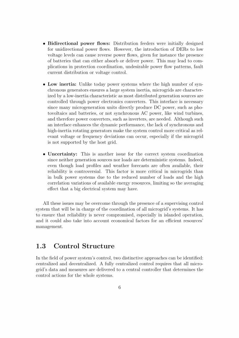
Regarding the secondary control layer, it implements a centralized controller inorder to both restore variables’ shifts and to efficiently manage microgrid energyflows. It should be noted that the frequency is required to be as close all possible to50 Hz. This is a more relevant issue if the islanded microgrid need to be reconnectedagain to the main grid; indeed the two systems must be synchronized at the samenominal frequency and phase at the interconnection point. To accomplish thistask, an integrator is first placed on the frequency error, so as to guarantee azero steady-state frequency error. Then, a Model Predictive Controller (MPC)is designed. This control strategy is based on a detailed and structured theorybut, to put it briefly, this control algorithm performs an optimization process on apredefined time span so that the optimal control variables are chosen. Moreover,weather and load profiles forecasts are usually available and they could be used toperform a more accurate optimization over a defined prediction horizon.

Although the system has a continuous dynamics, it has been quantized intoa discrete-time based system. The sampling time can be arbitrary decided butthere are however some limitations. In fact, a too slow control action could notbe enough effective, while it may be not possible to implement a too fast one dueboth to computational limits and to the fact that it is assumed that the primarydynamics have already reached the steady-state condition. Therefore, the timeframe is chosen to be in the order of some minutes. All the details regardingthis solution will be extensively discussed in next chapters, explaining both thetheoretical definition and the actual implementation. However, in order to have afirst insight of the proposed hierarchical control structure, a simplified scheme isreported in Figure 1.4.

Figure 1.4: Proposed control scheme

11

1.6 Thesis Outlook

The thesis is structured as follows.

After this introduction, the second chapter will focus on a detailed descrip-tion of the issues that involve the islanded condition. An overview of the primarycontrol theory will be also given, explaining how its implementation can actuallygive a first resolution to the mentioned issues. It will be shown that different pri-mary control configurations exist and their implementations actually depend onthe network parameters and loads. However, as already mentioned, a primary con-trol layer is not enough to efficiently manage an islanded microgrid and thereforean additional and more complex control layer is needed.

Since the secondary control layer is based on the Model Predictive Controltheory, a mathematical model of the system is needed. The third chapter willshow how the network model has been derived starting from the power flow the-ory. Moreover, also the main microgrid elements need to be modeled so that thecorresponding main variables can be taken into account during the optimizationprocess. Finally, the system simulator developed by RSE S.p.A. will be presented.

Once the system model has been presented, the fourth chapter will be focusedon the actual design of the secondary control layer. The prediction approach willbe described and the implemented cost function and variable constraints will bediscussed in details.

Starting from the designed hierarchical control structure, its performances willbe analysed in the fifth chapter. Firstly, the microgrid test case, as well as itsmain elements, will be described. Then, the effectiveness of the defined controlsystem will be shown through several simulations. Additional tests will be alsoperformed, taking into account more realistic implementations and features of thedesigned control framework.

Finally, a chapter will cover some conclusive considerations about the treatedcontrol problem, showing also the additional features which could be investigatedin future research developments.

12

Chapter 2

Primary Control

2.1 Islanding Issues

The Tellegen’s theorem states that the sum of the generated, lost and absorbedpower in an electrical network must be always equal to zero [16]. This is formalizedin (2.1) and (2.2) by considering separately active (P) and reactive (Q) powers.

n∑k=1

P generatedk +

n∑k=1

P lostk +

n∑k=1

P absorbedk = 0 (2.1)

n∑k=1

Qgeneratedk +

n∑k=1

Qlostk +

n∑k=1

Qabsorbedk = 0 (2.2)

where n corresponds to the number of nodes of the network 1.

In grid-connected mode this theorem is always valid since any unbalance be-tween generated and absorbed power is compensated by an energy import or exportfrom/to the main grid. On the other hand, the islanded operating mode becomesa critical situation for the absence of grid-connection and because generated andabsorbed powers easily mismatch due to the intermittent and stochastic nature ofmost renewable sources.

It should be noted that the electrical power, especially if related to transmissionlosses and to loads, is not a fixed quantity but it depends on the network variablessuch as voltages (V ), currents (I ) and frequency (ω).

1 An electrical network can be represented by a graph where nodes correspond to eithergeneration or load units and branches correspond to the interconnections between utilities.

13

Because of this, it would be more correct to rewrite equations (2.1) and (2.2)as reported in (2.3) and (2.4), explicating the dependence of the powers from thenetwork variables. Moreover, at steady state the whole network reaches a uniquesystem frequency, therefore it is not defined as a nodal variable, like voltages, butit is a global variable. It is important to underline that, since lost powers aremainly related to line losses, they do not depend only on the electrical variablesof their own node but they are defined from the voltages of all the interconnectednodes, as well as from the system frequency.

n∑k=1

P generatedk (Vk, ω) +n∑k=1

P lostk (V1, ..., Vn, ω) +n∑k=1

P absorbedk (Vk, ω) = 0 (2.3)

n∑k=1

Qgeneratedk (Vk, ω) +n∑k=1

Qlostk (V1, ..., Vn, ω) +n∑k=1

Qabsorbedk (Vk, ω) = 0 (2.4)

The dependence between powers and network variables has a considerable im-pact on the management of an islanded microgrid. Since the Tellegen’s theoremmust always be verified, it happens that when an unbalance occurs, for exampledue to a sudden load peak, voltages and microgrid frequency naturally vary bring-ing the system to a new equilibrium condition where the sum of powers is againzero. However, depending on the size of the unbalance, microgrid voltages andfrequency may largely deviate from their reference values, resulting in an equilib-rium condition that is not allowed for the system correct operation. In low voltagegrids (LV grids) the network variables have to respect some predefined limitationsto not compromise the power quality, as well as to not damage microgrid physicaldevices.

The Italian Electrotechnical Committee (CEI) defined several regulations forpower quality of low voltage networks [12]; however they are mostly related tomicrogrids in grid-connected mode since the islanding mode is quite a new concept.A norm that can be applied in the islanded case is the CEI 8-6 [13], that is relatedto the power quality of low voltage networks in real geographic islands; these infact do not have a connection with the main grid if located too far from the shore.The defined requirements are:

f = 50 Hz ± 2%

V = 400 V ± 10%

where f corresponds to the microgrid frequency and V to the amplitude of theline-to-line voltage in three-phase interconnections. This means that the frequencycan deviate only by 1 Hz around the nominal value, while line voltages are boundedbetween 440 V and 360 V.

14

Given the aforementioned issues, a primary control level is designed to limitthe variables’ deviations. Practically, this control layer consists in a decentralizedstructure that quickly modifies the generated power of each source so that thenetwork power balance becomes feasible without making voltages and frequencyreach values that are not allowed by the regulations. This primary control schemeis composed of two sub-layers: the inverter output control and the droop control.

2.2 Inverter Output Control

Figure 2.1: Inverter simplified circuit

The inverter represents one of the most used power converters and it is designedto transform a DC power source into an AC one. Even though the literatureprovides a detailed description of its physical structure and control [14], it is notof interest for this work to go into a detailed explanation. To put it briefly, theinverter circuit consists in a series of switching valves and diodes (see Figure 2.1)that, through an accurate control, can generate a three-phase sinusoidal voltagewaveform from a DC power source. Moreover, there are some configurations thatimplements also an AC/AC conversion through the sequence of an AC/DC stageand a DC/AC stage; in this way it is possible to decouple two distinct AC powerswhich can have different frequencies, as well as different voltage magnitudes.

Given the potentialities of these power converters, they will become fundamen-tal devices for future microgrids. This is confirmed by the fact that some generationsources produce DC power, such as energy storage units and photovoltaics, whileothers, such as wind turbines, produce AC power that is not synchronous with thegrid frequency. Moreover, this interface allows also to independently control theoutput power or voltage waveform of each source, based on the set-points imposedby the droop control. To accomplish this task, a series of cascade loops and mod-ulation techniques are designed that act on the inverter switching valves in orderto track the chosen output variable, such as the output voltage or current [14].

15

Depending on the selected controlled variable, two inverter control strategiescan be adopted for distributed energy control: the Voltage Source Control (VSC)and the Current Source Control (CSC).

The Voltage Source Control aims to feed the grid with a predefined voltagewaveform by imposing the output voltage magnitude and frequency. In this case,depending on the load power and on the power losses, the resulting generatedactive and reactive power are defined. The actual control is implemented withthe d-q frame-based voltage controller and a inner current loop that tracks thepredefined values of iod and ioq [15].

As far as the Current Source Control is concerned, it has an opposite pur-pose since the inverters are controlled to provide predefined values of active andreactive powers (this configuration is also called PQ control). The inner controlloop consists in a current and a voltage control loop that provide the values ofiod and ioq in order to generate the power values imposed by the droop con-trol [17]. In this case, the inverter output voltage magnitude and frequency arenot predefined but they come from the network power balance equations since, asstated before, the network variables will assume the values that ensure the validityof Tellegen’s theorem.

Having decided whether the inverter is controlled as a voltage source or acurrent source, then another sub-layer needs to be designed.

2.3 Droop Control

The droop method is an efficient and simple decentralized control strategy. Thislayer, having no need of intercommunications with other units and being character-ized by a proportional control action, ensures a rapid control action that minimizespower unbalances and consequently the system frequency and voltages. This is arelevant feature since, as stated in the first chapter, the inverter interface impliesa low system inertia, resulting in fast dynamics that must be properly managed.

Although the droop proportional actions have not a unique definition, theyare implemented such in order to link the network variables’ deviations and thegenerated powers’ deviations from their nominal values. In other words, this con-trol layer varies a defined network variable, such as the inverter output frequency,based on the variation of another electrical variable, such as the actual generatedactive power. The dependency between the variables that motivates the controlaction will be furtherly discussed in the following paragraph.

16

2.3.1 Droop Relationships

There are three possible droop couplings: the resistive, the inductive and the mixedrelationship.

• Resistive: The active power variation is linked to the nodal voltage one,while the reactive power variation to the network frequency one (P-V, Q-ω).

• Inductive: The active power variation is linked to network frequency one,while the reactive power variation to the nodal voltage one (P-ω, Q-V).

• Mixed : In this case both active and reactive power variations have an impactboth on frequency and voltages; although this can express more realisticcases, this relationship is not very used given its complex definition.

The droop relationships are usually chosen based on the line impedances [18],and, in particular, the key factor is represented by the ratio between resistive andthe inductive impedance of the line, known as the R/X factor. A network char-acterized by lines with small values of the R/X factor is said to have a mainlyinductive characteristic and suggests to exploit, for the droop control, the activepower - frequency and reactive power - voltage relationship. On the other hand,large values of the R/X factors result in stronger correlations between active powerand voltage and between reactive power and frequency. Being the resistive char-acteristic is typical of small grid systems like the one considered in this work, theresistive droop relatioship will be considered.

Although a rigorous proof of the reasons why the resistive and the inductiverelationship impose these precise links would be beyond the purpose of this work,a shorter intuitive explanation can be given considering the simple case reportedin Figure 2.2.

Figure 2.2: Simple electrical network

17

The network is composed of one generator and one load, interconnected througha line with a defined impedance. It is assumed that this AC network has alreadyreached the steady state condition, therefore each variable has a sinusoidal wave-form that pulsates at a steady-state frequency, ω. This allows to study the systemin the phasor domain, where each voltage can be represented in the complex planeas a phase vector that rotates at the steady-state frequency [19], as reported inFigure 2.3.

Figure 2.3: Phasor representation of nodal voltages

Node 1 is assumed to be the reference node, called also slack node. This meansthat all phase vectors are defined with respect to a new coordinate system (α, β),which is synchronous and aligned with V1. Therefore:

V1αβ

= V1

V2αβ

= V2 ej δ21

Given the nodal voltages and the line impedance, the line current can be easilycomputed:

I1αβ

=(V1

αβ − V2αβ

)

R+ jX=

(V1 − V2 cos(δ21)− j V2 sin(δ21) )

R+ jX=

=−R V2 cos(δ21) +R V1 −X V2 sin(δ21)

R2 +X2+

+ jX V2 cos(δ21) −X V1 −R V2 sin(δ21)

R2 +X2

18

Knowing both voltage and output current of Node 1, now it is possible tocompute the complex delivered power:

S1 = V1αβ · (I1

αβ)∗ = V1

(R (V1 − V2 cos(δ21)) −X V2 sin(δ21))

R2 +X2+

+ j V1(X (V1 − V2 cos(δ21)) +R V2 sin(δ21))

R2 +X2

Finally, the output active and reactive power are computed by consideringseparately the real and the imaginary part of the complex power:

P1 = Re(S1) = V1(R (V1 − V2 cos(δ21)) −X V2 sin(δ21))

R2 +X2

Q1 = Im(S1) = V1(X (V1 − V2 cos(δ21)) +R V2 sin(δ21))

R2 +X2

Starting from the expressions of the active and reactive generated power withthe explicit dependence on the network variables, now it is possible to understandwhy the resistive and the inductive relationships have these precise links betweenpowers, frequency and voltages. Considering first the inductive droop coupling: itis applied when the network R/X factor is very small. Therefore, by consideringX � R and by linearizing around δ21 ' 0 (in a single line interconnection it canbe assumed that voltages have nearly the same phase), we obtain:

P inductive1 = − (

V2 V1 X

R2 +X2) δ21 (2.5)

Q inductive1 = V1

(V1 − V2) X

R2 +X2(2.6)

While for a resistive network, where R� X, it results that:

P resistive1 = V1

(V1 − V2) R

R2 +X2(2.7)

Q resistive1 = (

V2 V1 R

R2 +X2) δ21 (2.8)

By looking to the equations (2.5) and (2.8), it is possible to see that an incre-ment in the phase difference between the two nodes has an impact on the active

19

power in the inductive case and on the reactive power in the resistive case. Ac-tually, the phase difference is strictly related to the frequency. An increase of δ21

means that V2 waveform tends dynamically to anticipate the V1 one, which in turnimplies that the frequency of Node 2 tends to be higher with respect to Node 1[20]. Therefore, in order to control the frequency, for inductive microgrids it isbetter to vary the generated active power, while for the resistive case it is betterto act on the variation of reactive power.

Regarding the voltages, it should be noted that there is not a perfect decouplingsince a voltage variation affects both the active and reactive powers. However, insome cases, such as in (2.6) and in (2.7), there is a squared dependence fromthe generation voltage V1 and the relative power. Although the effects are notcompletely decoupled as for the frequency, in the inductive case the generationvoltage is linked with the delivered reactive power, while in the resistive case thegenerated active power is usually used to control the nodal voltage.

The explained relationships are not perfectly decoupled; however, for the sakeof simplicity the droop is always designed as it had separate effects on the differentvariables. This approximation is well accepted since the aim of droop control isnot to perform a precise control action but only to allow the network to properlywork without large deviations of variables.

Remark: For small scale networks it is not true that only line impedances have tobe taken into account, but the whole system should be considered. Actually, sincemicrogrids are characterized by short lines, load characteristics have a great impacton the relationships between network variables and generated powers. There aresome loads, such as linear RLCs, that are characterized by a resistive coupling (P-V, Q-ω), while others, such as asynchronous rotating motors, show an inductiverelationship (P-ω, Q-V). Depending on the prevailing load characteristics, thedroop coupling should be chosen. Taking into account the experiments carried outin [20], it can be stated that the resistive relationship is the one that ensures thesystem stability for most types of microgrids. Actually, it is quite difficult to havea small-scale network characterized by a prevailing inductive characteristic, sinceit is not frequent to have rotating loads directly connected to the line but they areusually interfaced through inverters.

Having chosen the droop relationships that link the variations of powers to thevariations of voltage and the frequency, there are however different droop controlapproaches. Although they all have the same objective, they are based on differentcontrol actions. In the following section a more detailed explanation is given.

20

2.3.2 Droop control strategies

Depending on the chosen controlled and control variables, two droop methods canbe adopted: the Conventional and the Inverse Droop.

The Conventional Droop relies on a direct action since, through proportionalgains, it varies directly the output voltage magnitude and frequency based onthe variation of the delivered active and reactive power. This droop strategy isinterfaced with inverters controlled as voltage sources (VSC). Indeed, as the drooplayer defines the output voltage waveform, its magnitude and frequency are thensent as set-points to the inverter output control (see Figure 2.4).

On the contrary, the Inverse Droop control acts in an opposite way. It mod-ifies the generated output power depending on the deviations of nodal voltagemagnitude and frequency from their nominal values. This droop strategy is usu-ally implemented together with Current Source Controlled inverters, since theyare able to track active and reactive power set-points. As stated before, withthis approach it is not possible to have a direct control on the voltages and onthe microgrid frequency, but they will take the values that guarantee the powerbalance. A schematic representation of the Inverse Droop Control with resistiverelationship is reported in Figure 2.5.

Figure 2.4: Conventional Resistive Droop

21

Figure 2.5: Inverse Resistive Droop

2.4 Primary control design

After this brief overview on the possible primary control structures, a descriptionof the scheme considered in this work is now given.

It consists in a decentralized structure where at each generation node an InverseDroop control is located, therefore all generation inverters are controlled as currentsources. This implies that there is not a direct control of the network variables,but they will assume the values that make the power balance feasible. Moreover,the resistive relationship (P-V, Q-ω) is implemented since, as aforementioned, itallows the network stability for most types of loads.

Therefore, the output powers are defined by the droop control as:

P genj = mvj ∗ (Vi − V nom) + P gen refj (2.9)

Qgenj = mωj ∗ (ω − ωnom) + Qgen refj (2.10)

22

where j ∈ (1, ..., ncg), with ncg number of controllable generation units,V nom = 400 V and ωnom = 314.16 rad/s (i.e. 50 Hz), while mv

j and mωj correspond

to the droop proportional gains. Then, the final values of P genj and Qgen

j are sentto the inverter output control that is in charge of delivering the defined active andreactive generated powers.

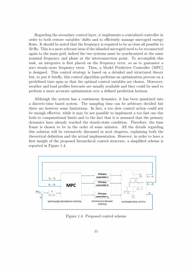
Regarding the proportional gains, their definition is shown in Figure 2.6, wherethey correspond to the slopes of the droop characteristics.

Figure 2.6: Implemented droop characteristics

It is worth noticing that the functions have not constant slopes. Indeed, gen-erators have limited power capabilities and therefore for some values of frequencyand voltage magnitude the output powers are saturated to their working limits.

The two droop functions have opposite effects on the outputs. On the onehand, the active power is decreased with the respect the reference value as thevoltage deviation increases, while the reactive power offset is directly proportionalto the frequency variation. An intuitive explanation of this choice can be givenby considering a resistive network with a generator and a parallel RLC load (seeFigure 2.7).

In order to study the network, the absorbed power is firstly computed. Sincemicrogrids are characterized by short interconnections and loads represent themost relevant power absorption, power line losses are neglected.

23

Figure 2.7: Simple network

Z = R + jωL +1

jωC

Sload = V load (I load)∗ = V load (V load

Z∗) =

(V load)2

R+ j (

(V load)2

ωL− ωC(V load)2)

P load = Re (Sload) =(V load)2

R(2.11)

Qload = Im (Sload) =(V load)2

ωL− ωC(V load)2 (2.12)

Through the equations (2.11) and (2.12), it is possible to give an explanation ofthe droop characteristics shown in Figure 2.6. Taking into account firstly the activepower, if a generation peak occurs, there will be an initial unbalance where thegenerated power exceeds the absorbed one (P gen > P load). Given the Tellegen’stheorem, this will result in a voltage increase since it is the only way to raisethe active absorbed power, as reported by equation (2.11). At steady-state, thecondition P gen = P load will be reached. However, if the initial difference betweenthe generated and absorbed power is big, the voltage will largely deviate from itsnominal value. To overcome this issue, it is needed to implement a control systemthat automatically decreases P gen as the nodal voltage exceeds its nominal value.In this way in fact, the unbalance between absorbed and generated power willbe reduced and therefore the final equilibrium condition can be reached withoutrelying on a large voltage deviation. This is exactly how the designed droop controlacts, as reported in the left graph of Figure 2.6. Indeed, if the voltage has a valuebeyond the nominal one, the generation active power is reduced with respect toits reference value.

24

The same reasoning can be carried out regarding reactive powers. Indeed, ifan unbalance occurs so that Qgen > Qload, the absorbed reactive power need to beraised in order to fulfill the Tellegen’s theorem. As reported by (2.12), an incrementof Qload can be achieved by a frequency drop. Also in this case, the reachedequilibrium could not be allowed by the regulations or it can damage physicaldevices. Therefore, as the frequency goes down, the droop control decreases alsothe generated reactive power so that the power balanceQgen = Qload can be reachedwithout having a frequency large steady-state shift. This behavior is coherent withrespect to the right graph in Figure 2.6, where reactive power and frequency showsa proportional relationship.

Although the adopted droop strategy has been justified in a simple case, it canbe extended to a more structured microgrid equipped with many generators andloads. As reported in [20], the inverse resistive droop control implemented as inFigure 2.6 ensures the network stability for many types of loads, even though itdoes not impose a direct control on voltage magnitudes and frequency.

2.5 Conclusions

The designed primary control allows the system to properly work in islanded mode,even though power unbalances may occur. However, a control action based onlyon proportional gains does not ensure that the variables reach their nominal val-ues [11], which is a desirable aspect especially for the frequency. Moreover, atthis stage the droop active and reactive power references are fixed parameters(see Figure 2.6). It would be surely better to have an additional control systemthat efficiently varies the power references depending on the actual microgrid ab-sorption.

Indeed in this way, power unbalances will be of limited size and consequentlythe variables’ steady-state deviations will be reduced. Finally, relying only on aprimary control layer, each source is independently controlled and so it is not pos-sible to have a high-level coordination between sources. This would be a relevantfeature since it allows to implement several strategies based either on economicalreasons or on green energy-oriented policies.

All the mentioned issues can be overcome by a supervising control layer, im-plemented as a centralized secondary controller. Its control action would consistin shifting the droop characteristics by varying P gen ref and Qgen ref based on anoptimization algorithm. This structure, if properly designed, can achieve relevantresults in terms of network stability and efficient resource management.

25

Chapter 3

Microgrid Mathematical Modeland Simulator

3.1 Introduction

The purpose of the secondary control is both to restore the network variables’ de-viations and to efficiently manage the microgrid energy flows. The chosen strategyis based on the Model Predictive Control approach (MPC), which is a control algo-rithm which performs a recursive optimization process over a predefined predictionhorizon. As underlined in the previous chapter, this control will be designed tovary the power references of the controllable sources, taking into account the ac-tual state of the network variables. Furthermore, since the network frequency isconsidered the most critical variable, an integrator has been placed between thefrequency error and the centralized MPC controller, so ensuring zero static error.

In order to design the secondary control layer, the state-space model of thewhole microgrid, including the primary layer, is needed. Before developing it,at the secondary stage the primary control dynamics have been considered to bealways at steady state, therefore represented by the droop final static relationships.This is an acceptable assumption since the inverter interface allows to have relativesmall time constants. Moreover, since the primary layer reaches the steady-statecondition in about 10 seconds and the centralized secondary control is based ona complex optimization algorithm, the variables’ sampling time for the secondarylayer can not be relatively small but it has to be at least one minute. The developedmicrogrid model has been chosen to be defined by a discrete time-based system,where the sampling time corresponds precisely to the discrete time step tk.

26

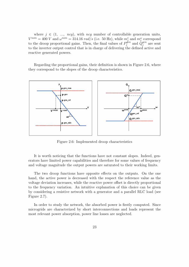
By looking at Figure 3.1, it is possible to understand how the designed controlsystem works. Actually, every tk the network variables are sampled and the MPCalgorithm starts its optimization process. After a computation time of few secondsτc, the optimization process ends and so the control actions are applied, whichmeans that the MPC varies the reference powers of the droop functions. Then, theprimary network layer starts its transient and it reaches the steady state conditionin a settling time τn of some seconds. Recursively, at the next step the steadystate variables’ values are sampled and the MPC is performed again in order to thedecide the next reference power variations. It should be noted that communicationtimes between the different units are neglected, they are in fact relatively smallwith respect to the other time frames.

Figure 3.1: Time Discretization

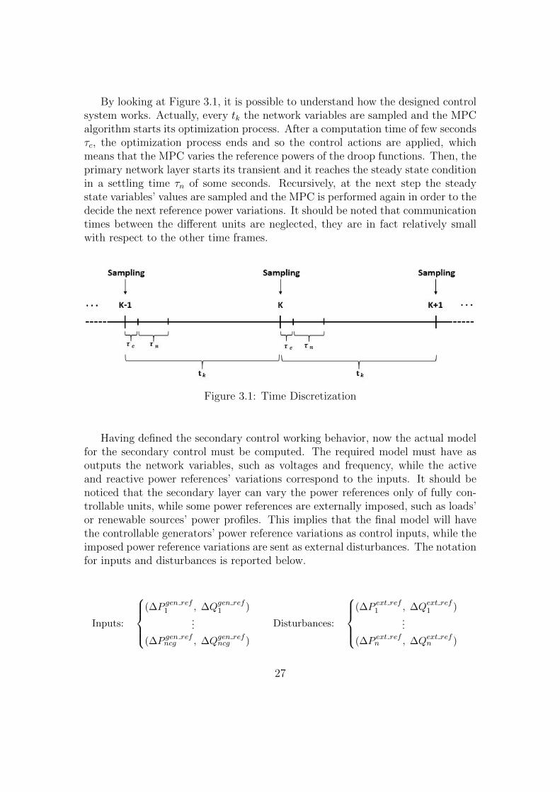
Having defined the secondary control working behavior, now the actual modelfor the secondary control must be computed. The required model must have asoutputs the network variables, such as voltages and frequency, while the activeand reactive power references’ variations correspond to the inputs. It should benoticed that the secondary layer can vary the power references only of fully con-trollable units, while some power references are externally imposed, such as loads’or renewable sources’ power profiles. This implies that the final model will havethe controllable generators’ power reference variations as control inputs, while theimposed power reference variations are sent as external disturbances. The notationfor inputs and disturbances is reported below.

Inputs:

(∆P gen ref1 , ∆Qgen ref1 )

...

(∆P gen refncg , ∆Qgen refncg )

Disturbances:

(∆P ext ref1 , ∆Qext ref1 )

...

(∆P ext refn , ∆Qext refn )

27

where ncg corresponds to the number of controllable generation units, while thedisturbances are modeled to be 2n, defining the external power reference variationfor each node (if a node is not affected by an imposed power variation, the relativedisturbance will be always zero).

An overview of the overall control scheme, with a particular evidence of thesystem model that need be computed, is reported in Figure 3.2.

Figure 3.2: Hierarchical control block diagram

The developed system model will be based on the power flow analysis 1 adaptedto an islanded network. To better understand its definition, a brief overview ofthe power flow theory is firstly given.

3.2 Power Flow

The purpose of this approach is to have a complete insight of the powers flowing outfrom each node in an AC grid system. Taking into account the case issued in thiswork, it corresponds to a steady-state network characterized by balanced three-phase interconnections. This means that the phasor approach can be adopted,which identifies for each node a single voltage waveform corresponding to the lineto line voltage.

1Also known as ”load flow” study

28

The voltages are represented with phase vectors, where the magnitude corre-sponds to the amplitude of the waveform, while the vector phase represents thephase shift with respect to the coordinate system aligned to the reference node,called slack node. This implies that the vector phase angle of the slack nodalvoltage is always zero. When microgrids are in grid-connected mode, the referencenode coincides the point of common coupling, while its location can be arbitrarilychosen in the islanded condition.

The first step to perform the power flow analysis is to define the microgridphysical characteristics and this is done through the admittance matrix. Thismatrix contains all the information regarding the network impedances, includingthe loads’ and generators’ ones. However, in this case the network characteristicsare not expressed in terms of impendances but through the admittance concept,that is defined as the inverse of the impedance. The matrix construction is wellexplained and documented in the literature, coming from the theory of two-portnetworks [21].

Its final structure is:

[Y]ij =

{yii +

∑nk=1, k 6=i yik if j = i

−yij otherwise

where, if j 6= i, yij represents the line admittance from node i to node j,otherwise if j = i, yii is referred to the nodal admittance of node i itself, for instancerelated to the presence of the load impedance. It is important to underline that,given the presence of the inductive and capacitive impedance, the line admittancehas not a fixed value but it depends on the network frequency. This implies that,like powers, also the admittance matrix varies as network variables deviate.

Having defined the admittance matrix, it is possible to compute the explicitexpression of the powers flowing out from each node. Being V the vector of allnodal voltage phasors, I the vector of all nodal output current ones and S thevector of all nodal complex powers, the active and reactive powers are determined.

I = Y V

S = V I∗

PT = Re(S)

QT = Im(S)

29

After performing all calculations, the vectors PT and QT result to be:

P Ti (V(1...n), δ(1...n), ω) = Vi

n∑j=1

[ Vj ∗ (Re(Yij(ω)) ∗ cos(δi − δj) +

+ Im(Yij(ω)) ∗ sin(δi − δj) ] (3.1)

QTi (V(1...n), δ(1...n), ω) = Vi

n∑j=1

[ Vj ∗ (Re(Yij(ω)) ∗ sin(δi − δj) +

− Im(Yij(ω)) ∗ cos(δi − δj) ] (3.2)

Through these equations and by knowing the steady-state values of frequency,phase angles and voltages, it is possible to have an exact evaluation of powersflowing in the considered network.

In an electrical network, each node can be characterized by the presence eitherof a controllable generation unit, e.g. a battery, or of an uncontrollable one, e.g.a load. By defining the power balance at each node, it follows that the activeflowing out power is equal to the difference between the active power injectedby a controllable generation unit (P gen) and the active power absorbed by anuncontrollable one (P ext), as depicted in Figure 3.3.

Figure 3.3: Nodal Power Balance

Looking to the above figure, P genj corresponds to the active power that the jth

generator injects on the ith node. It is assumed that a generator can provide poweronly to the node where it is placed. On the other hand, P ext

i represents the activepower that is absorbed or generated by an uncontrollable unit and it is modeledfor each ith node. Obviously, if the ith node is not characterized by the presence ofan external power disturbance, the relative P ext

i will be zero. The above describedreasoning holds also for the reactive powers.

30

Putting the nodal balance into equations, it results that for each node i thefollowing equations hold:

{P Ti (V(1...n), δ(1...n), ω) = P genj (Vi, ω) − P exti (Vi, ω)

QTi (V(1...n), δ(1...n), ω) = Qgenj (Vi, ω) − Qexti (Vi, ω)(3.3)

As aforementioned, by applying the power flow analysis to the islanded mi-crogrid case, it is possible to develop a system model that, taking as inputs thereference nodal powers, gives the network voltages, phase angles and frequency.This will be described in the next section.

3.3 Network Model

The first step to develop the network model is to define all the nodal powers as thesum of a constant quantity (i.e. the reference nodal power) plus a variation due tothe impact that the nodal voltages and the frequency have on the related power.This is a true assumption both for generators, where the droop control introducesa power variation because of network variables’ deviations, and for loads, since inmost cases loads show a dependence between the absorbed power and the networkvariables, as discussed in paragraph 2.4.

Therefore, for each generator it follows that:

{P genj (Vi, ω) = P gen refj + ∆P genj (Vi, ω)

Qgenj (Vi, ω) = Qgen refj + ∆Qgenj (Vi, ω)(3.4)

With regard to the externally imposed powers (such as loads and renewablesources), since they have been modeled for each node, the same equations can bespecified.

{P exti (Vi, ω) = P ext refi + ∆P exti (Vi, ω)

Qexti (Vi, ω) = Qext refi + ∆Qexti (Vi, ω)(3.5)

31

By putting together (3.3), (3.4) and (3.5), the following holds:

{P gen refj − P ext refi = P Ti (V(1...n), δ(1...n), ω) − ∆P genj (Vi, ω)−∆P exti (Vi, ω)

Qgen refj − Qext refi = QTi (V(1...n), δ(1...n), ω) − ∆Qgenj (Vi, ω)−∆Qexti (Vi, ω)

For the sake of simplicity, from now on, single active and reactive power refer-ence P ref

i , Qrefi are defined for each node. If in the same node both a generator

and a load are present, the overall power references will be defined as the differencebetween the generated and the externally imposed reference power.

Therefore, equations (3.6) follow, which actually express how the nodal refer-ence power are linked to the network variables.

{P refi = P Ti (V(1...n), δ(1...n), ω) − ∆P genj (Vi, ω)−∆P exti (Vi, ω)

Qrefi = QTi (V(1...n), δ(1...n), ω) − ∆Qgenj (Vi, ω)−∆Qexti (Vi, ω)(3.6)

It should be noted that the above equations are 2n, where n corresponds to thenumber of nodes of the network. Regarding the variables, the number of consideredphase angles is (n− 1) since the slack node phase is always zero. Therefore, withn nodal voltages, (n − 1) phase angles and 1 microgrid frequency, 2n networkvariables can be identified.

Given the expressions of flowing powers in (3.1) and (3.2), the equations (3.6)are obviously nonlinear. It is recalled that the developed network model willbe fundamental for the secondary control layer to perform the optimization pro-cess; moreover, the base formulation of the MPC approach is referred to linearmodels. To overcome this issue, the secondary controller will sample the steady-state values of the network variables at each control iteration and it will per-form a linearization process so that a linear model is obtained. By consideringthe steady-state values of the network variables as the actual equilibrium pointx = (V1, ..., Vn, δ2, ..., δn, ω), the equations (3.6) can be actually linearizedthrough through a first-order Taylor series approximation.

∆P refi = ( ∂

∂V Prefi )t

∣∣∣∣x

∆V + ( ∂∂δP

refi )t

∣∣∣∣x

∆δ + ( ∂∂ωP

refi )t

∣∣∣∣x

∆ω

∆Qrefi = ( ∂∂V Q

refi )t

∣∣∣∣x

∆V + ( ∂∂δQ

refi )t

∣∣∣∣x

∆δ + ( ∂∂ωQ

refi )t

∣∣∣∣x

∆ω

(3.7)

32

In equation (3.7), ∆V = (∆V1, ..., ∆Vn), ∆δ = (∆δ2, ..., ∆δn), and ∆ωcorrespond to the variations of the network variables with respect to the equilib-rium point x. On the other hand, ∆P ref

i and ∆Q refi expresses the reference power

variations with respect to P refi and Q ref

i , which in turns correspond to the nodalreference powers at the equilibrium point.

Expressing equations (3.7) in matrix form, it follows:

∆P ref1...

∆P refn

∆Qref1...

∆Qrefn

=

(∂P ref

i∂V )

∣∣∣∣x

(∂P ref

i∂δ )

∣∣∣∣x

(∂P ref

i∂ω )

∣∣∣∣x

(∂Qref

i∂V )

∣∣∣∣x

(∂Qref

i∂δ )

∣∣∣∣x

(∂Qref

i∂ω )

∣∣∣∣x

∆V1...

∆Vn∆δ2

...∆δn∆ω

The matrix containing all the power derivatives, called network Jacobian (J),must be evaluated at the actual equilibrium point x. This implies that it is not afixed matrix but it changes at each time step, depending on the reached steady-state equilibrium for the primary dynamic.

The model requested for the designing of the secondary controller must havethe network variables as outputs and the reference powers as inputs. Since weare dealing with a (2n x 2n) matrix, an inversion can be performed so that thenetwork variables are computed based on the reference power variations.

∆V1...

∆Vn∆δ2

...∆δn∆ω

=

(∂P ref

i∂V )

∣∣∣∣x

(∂P ref

i∂δ )

∣∣∣∣x

(∂P ref

i∂ω )

∣∣∣∣x

(∂Qref

i∂V )

∣∣∣∣x

(∂Qref

i∂δ )

∣∣∣∣x

(∂Qref

i∂ω )

∣∣∣∣x

−1

∆P ref1...

∆P refn

∆Qref1...

∆Qrefn

33

At this stage, a static relationship between the reference power variations andthe network variables ones with respect to the equilibrium point is obtained. Sincethe variation of the reference power implemented by the secondary controller hasan effect on the network variables and since the consequent steady-state valueswill be sampled at the next time step, the discretized model is formulated byconsidering a 1-step shift between the cause and the effect.

Therefore it becomes:

∆V1(k + 1)...

∆Vn(k + 1)∆δ2(k + 1)

...∆δn(k + 1)∆ω(k + 1)

=

(∂P ref

i∂V )

∣∣∣∣x(k)

(∂P ref

i∂δ )

∣∣∣∣x(k)

(∂P ref

i∂ω )

∣∣∣∣x(k)

(∂Qref

i∂V )

∣∣∣∣x(k)

(∂Qref

i∂δ )

∣∣∣∣x(k)

(∂Qref

i∂ω )

∣∣∣∣x(k)

−1

∆P ref1 (k)...

∆P refn (k)

∆Qref1 (k)...

∆Qrefn (k)

where∆Vi(k + 1) = V (k + 1)− V (k)

∆δi(k + 1) = δ(k + 1) − δ(k)

∆ω(k + 1) = ω(k + 1)− ω(k)

{∆P refi (k) = P refi (k)− P refi (k − 1)

∆Qrefi (k) = Qrefi (k)−Qrefi (k − 1)

and x(k) corresponds to the primary steady-state values of network variables attime step k.

By computing the inverse of the Jacobian, the linearized system model dynam-ics can be obtained.

V1(k + 1) = V1(k) + α (1, 1) (k) ∆P ref1 (k) + ... + α (1, 2n) (k) ∆Qrefn (k)...

Vn(k + 1) = Vn(k) + α (n, 1) (k) ∆P ref1 (k) + ... + α (n, 2n) (k) ∆Qrefn (k)

δ2(k + 1) = δ2(k) + α (n+1, 1) (k) ∆P ref1 (k) + ... + α (n+1, 2n) (k) ∆Qrefn (k)...

δn(k + 1) = δn(k) + α (2n−1, 1) (k) ∆P ref1 (k) + ... + α (2n−1, 2n) (k) ∆Qrefn (k)

ω(k + 1) = ω(k) + α (2n, 1) (k) ∆P ref1 (k) + ... + α (2n, 2n) (k) ∆Qrefn (k)

where αi,j(k) corresponds to the (i, j) element of inverted Jacobian, J−1(k).

34

It is recalled that not all power references are imposed by the secondary controlbut some of them come from load powers or undeterministic renewable energysources. The uncontrollable power references are modeled as external disturbances,considered as known if power profiles are assumed to be available.

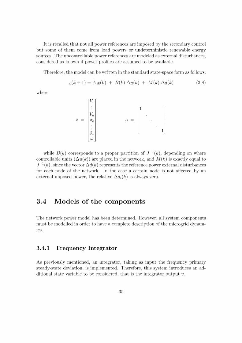
Therefore, the model can be written in the standard state-space form as follows:

x(k + 1) = A x(k) + B(k) ∆u(k) + M(k) ∆d(k) (3.8)

where

x =

V1...Vnδ2...δnω

A =

1

...

1

while B(k) corresponds to a proper partition of J−1(k), depending on wherecontrollable units (∆u(k)) are placed in the network, and M(k) is exactly equal toJ−1(k), since the vector ∆d(k) represents the reference power external disturbancesfor each node of the network. In the case a certain node is not affected by anexternal imposed power, the relative ∆di(k) is always zero.

3.4 Models of the components

The network power model has been determined. However, all system componentsmust be modelled in order to have a complete description of the microgrid dynam-ics.

3.4.1 Frequency Integrator

As previously mentioned, an integrator, taking as input the frequency primarysteady-state deviation, is implemented. Therefore, this system introduces an ad-ditional state variable to be considered, that is the integrator output v.

35

Figure 3.4: Frequency Integrator

Taking into account Figure 3.4, the integrator dynamics can be easily computedthrough the Z-transform [11].

V (z) =z

z − 1Eω(z)

Therefore, it follows:

(z − 1) V (z) = z Eω(z)

v(k + 1) = v(k) + eω(k + 1)

v(k + 1) = v(k) + ωnom − ω (k + 1)

v(k + 1) = v(k) + ωnom − ( ω (k) + Bω(k) ∆u(k) + Mω(k) ∆d(k) )

v(k + 1) = v(k) − ω (k) − Bω(k) ∆u(k) − Mω(k) ∆d(k) + ωnom (3.9)

where Bω(k) and Mω(k) correspond to the partitions of J(k)−1 related to thefrequency dynamics (last row of the Jacobian matrix). Moreover, the referencefrequency ωnom is included in the disturbance vector ∆d(k) since it is not a inputdecided by the secondary control.

The actual network model is then augmented with respect to its original for-mulation. Hence, by inserting equation (3.9) into (3.8), it results:

x(k + 1) = A x(k) + B(k) ∆u(k) + M(k) ∆d(k) (3.10)

36

where

x =

V1...Vnδ2...δnω

v

∆u =

∆P gen ref1...

∆P gen refncg

∆Qgen ref1...

∆Qgen refncg

∆d =

∆P ext ref1...

∆P ext refn

∆Qext ref1...

∆Qext refn

ωnom

and

A =

A0...0

0 . . . −1 1

B(k) =

b1,1(k) . . . b1,2ncg(k). . .. . .. . .

bn,1(k) . . . bn,2ncg(k)−bn,1(k) . . . −bn,2ncg(k)

M(k) =

m1,1(k) . . . m1,2n(k). . .. . .. . .

mn,1(k) . . . mn,2n(k)

0...0

−mn,1(k) . . . −mn,2n(k) 1

3.4.2 Batteries

Regarding the microgrid storage units, it can be assumed that they have an in-stantaneous power dynamics since the inverter time constants are negligible for thesecondary control time frame. The presence of batteries add however additionaldynamics related to their states of charge (SOC), which are function of the batteryactive power.

37

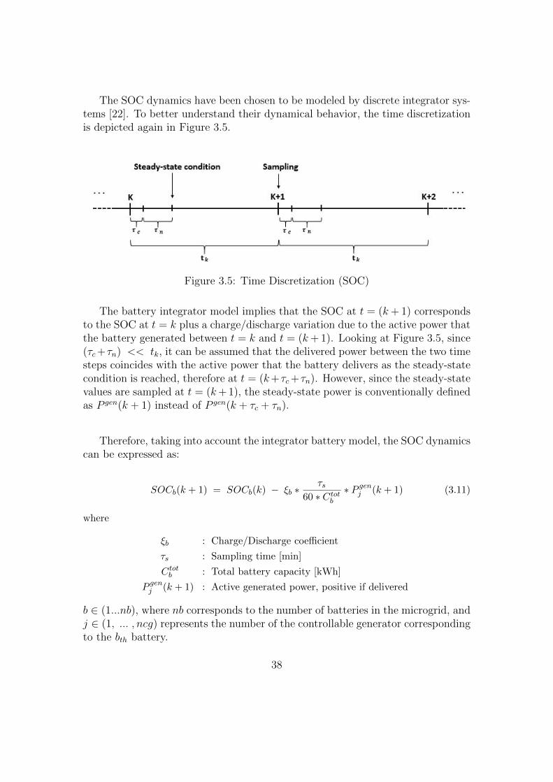
The SOC dynamics have been chosen to be modeled by discrete integrator sys-tems [22]. To better understand their dynamical behavior, the time discretizationis depicted again in Figure 3.5.

Figure 3.5: Time Discretization (SOC)

The battery integrator model implies that the SOC at t = (k+ 1) correspondsto the SOC at t = k plus a charge/discharge variation due to the active power thatthe battery generated between t = k and t = (k+ 1). Looking at Figure 3.5, since(τc+τn) << tk, it can be assumed that the delivered power between the two timesteps coincides with the active power that the battery delivers as the steady-statecondition is reached, therefore at t = (k+τc+τn). However, since the steady-statevalues are sampled at t = (k+ 1), the steady-state power is conventionally definedas P gen(k + 1) instead of P gen(k + τc + τn).

Therefore, taking into account the integrator battery model, the SOC dynamicscan be expressed as:

SOCb(k + 1) = SOCb(k) − ξb ∗τs

60 ∗ Ctotb∗ P genj (k + 1) (3.11)

where

ξb : Charge/Discharge coefficient

τs : Sampling time [min]

Ctotb : Total battery capacity [kWh]

P genj (k + 1) : Active generated power, positive if delivered

b ∈ (1...nb), where nb corresponds to the number of batteries in the microgrid, andj ∈ (1, ... , ncg) represents the number of the controllable generator correspondingto the bth battery.

38

The SOC dynamics need to be added to the microgrid model so that theycan be taken into account by the secondary control layer to perform an efficientresource management. However, the actual defined SOC model does not representa proper discrete dynamic since there is not a time shift between the final SOCand the relative delivered power. Moreover, at this stage the generated powers areunknown quantities since they are neither an input nor an output, but internalvariables of the system. Although the secondary scheme sets the power referencesfor the primary layer, the droop control then modifies the generated power basedon the network variables’ deviation. In order to add the SOCs to the state vectorx, the generated power dynamics must be previously defined.

Generated Powers Discrete Model

The generated active and reactive powers correspond to the sum of the actualpower reference plus the variation given by the droop primary control. This meansthat it can be written as:

P genj (k + 1) = P gen refj (k + 1) + ∆P droopj (k + 1)

Qgenj (k + 1) = Qgen refj (k + 1) + ∆Qdroopj (k + 1)

In this case, since the resistive inverse droop has been applied, ∆P droopj (k + 1)

will depend on the voltage deviation with respect to the nominal value, while∆Qdroop

j (k + 1) on the microgrid frequency one.

Therefore:

P genj (k + 1) = P gen refj (k + 1) + mvj (k + 1) ∗ (Vi(k + 1) − V nom) (3.12)

Qgenj (k + 1) = Qgen refj (k + 1) + mωj (k + 1) ∗ (ω(k + 1) − ωnom) (3.13)

where i corresponds to the node where the jth generator is placed.

In order to obtain the generated power dynamics, the state-space equationsshould be found so that it is possible to know the P gen

j (k + 1) and Qgenj (k + 1)

given the information at the time step k. Starting with the reference powersP gen refj (k + 1) and Qgen ref

j (k + 1), they are defined by pretty simple equationssince the reference power at (k + 1) corresponds to the reference powers at thetime step k plus the variation that the secondary control decided to implement.

39

Hence:

P gen refj (k + 1) = P gen refj (k) + ∆P gen refj (k) (3.14)

Qgen refj (k + 1) = Qgen refj (k) + ∆Qgen refj (k) (3.15)

In equations (3.11) and (3.12) the variables Vi(k + 1) and ω(k + 1) can besubstituted with the dynamics defined in paragraph 3.3. Regarding the droopparameters, it can be assumed that mv

j (k + 1) = mvj (k) and mω

j (k + 1) = mωj (k)

since the droop functions have been implemented with constant slopes.Therefore, (3.11) and (3.12) become:

P genj (k + 1) = P gen refj (k) + ∆P gen refj (k) + mvj (k) ∗ (Vi(k) +BVi(k) ∆u(k) +

+ MVi(k) ∆d(k) − V nom) (3.16)

Qgenj (k + 1) = Qgen refj (k) + ∆Qgen refj (k) +mωj (k) ∗ (ω(k) +Bω(k) ∆u(k) +

+ Mω(k) ∆d(k) − ωnom) (3.17)

From the equations (3.16) and (3.17), now it is possible to easily derive thestate-space equations since V nom and ωnom can be identified as known disturbances,while the remaining variables are either states or inputs.

Having defined the generated power dynamics, by putting equation (3.16) into(3.11), it results:

SOCb(k + 1) = SOCb(k) − ξb ∗τs

60 ∗ Ctotb∗ ( P gen refj (k) + ∆P gen refj (k) +

+ mvj (k) ∗ (Vi(k) +BVi(k) ∆u(k) +MVi(k) ∆d(k) − V nom) ) (3.18)

Now, the SOC dynamics can be added to the whole model since they areexpressed through a discrete model where all variables are either inputs or states,all known at t = k.

40

Remark: It should be noted that the obtained generated power dynamics mightnot be realistic in some circumstances. Firstly, it is not always true that mv

j (k +1) = mv

j (k) and mωj (k + 1) = mω

j (k), since, if the powers reach their limits, thedroop function slope becomes zero (see paragraph 2.4); this means that there couldbe some instants where mv

j (k + 1) 6= mvj (k) or mω

j (k + 1) 6= mωj (k). On the other

hand, the network model is based on a linearization process and therefore thevariables that the model computes at t = (k + 1) might have a slightly differentvalue from the real ones; indeed the linearized model at time t = k is valid onlyin the neighborhood of the system equilibrium point.

However, in spite of these approximations, these equations allow the secondarycontroller to have a good estimation of the effective generated power after theaction of the primary control, which is fundamental to estimate the charge ordischarge of the batteries.

By properly putting together all the analysed dynamics, it is possible to derivea final state-space equation that takes into account both the network variables,the generated powers and the batteries’ SOCs.

This is defined as:

˜x(k + 1) = ˜A(k) ˜x(k) + ˜B(k) ∆u(k) + ˜M(k) ∆˜d(k) (3.19)

where

˜x =

x

P gen ref1...

P gen refncg

Qgen ref1...

Qgen refncg

P gen1...

P genncg

Qgen1...

QgenncgSOC1

...SOCnb

∆u =

∆P gen ref1...

∆P gen refncg

∆Qgen ref1...

∆Qgen refncg

∆

˜d =

∆P ref1...

∆P refn

∆Qref1...

∆Qrefnωnom

V nom

41

while the complete structures of ˜A(k), ˜B(k), ˜M(k) are not reported for sim-plicity. However, they can be easily computed taking into account the dynamicsdefined in (3.14), (3.15), (3.16), (3.17) and (3.18).

3.4.3 Rotating Generators

The rotating generators dynamics have been neglected in the considered model, aswell their internal control loops. This means that it is assumed that the requestedpower by the hierarchical control structure will be immediately delivered by thegenerators. This is acceptable in our case since the time constants of controllablegenerators are much smaller with respect to the secondary control time frame.

3.4.4 Loads

Although the load units are not controllable by the secondary controller, their in-ternal models are needed in order to describe how the network variables influencethe absorbed power. As far as parallel RLC loads are concerned, the correspond-ing static model has been already introduced in paragraph 2.4, where the activeand reactive power expressions have been computed as functions of the networkvariables.

However, for more complex loads it quite difficult to mathematically com-pute these expression since there are not detailed information about their internalimpedances. Because of this, identification experiments are performed in order tofind static expressions defining how the absorbed powers depend on the load out-put voltage and frequency. These models are usually characterized by nonlinearfunctions, and their general structure is depicted in (3.20).

{P loadi = hp · fpv (Vi, kpv) · fpω (ω, kpω)

Qloadi = hq · fqv (Vi, kqv) · fqω (ω, kqω)

(3.20)

where fpv, fpω, fqv, fqω correspond to the predefined nonlinear functions thatexpress the static model used in the identification experiment. On the contraryhp, hq, kpv, kpω, kqv, kpω are parameters that need to be identified and they dependon the actual load characteristics.

42

The first two parameters are related to the amount of active and reactivepower that the load absorbs at nominal conditions, while the others are referredto dependence that the final absorbed power has on the corresponding networkvariable. Moreover, the load models are defined such that the parameters kpv,kpω, kqv, kpω are set to zero if the load does not show a dependence between thecorresponding power and the network variable.

For instance, if we want to define a model for a RLC load through the aboveequations, the parameter kpω must be set to zero since there is not a dependencebetween the active power and the network frequency, as reported by equation(2.13).

Although the knowledge of these models is not always available, they are fun-damental to choose the droop coupling to implement. Indeed, through their defi-nitions and the line characteristics is possible to estimate which is the prevailingimpedance of the network.

Having defined the models of the main system dynamics, now a brief descriptionof the implemented simulator is given.

3.5 Simulator

In order to test the control performances of both the primary and the secondarycontrol, a simulation environment must be developed. To do that, the MATLABTM

programming code has been used, thanks for its potentialities for system modellingand control. Regarding the microgrid components, they have been simulated byactually implementing the previous developed dynamics. On the other hand, thenetwork model is a nonlinear system and so it must be simulated through numericalmethods.

It is possible to find many network simulators in the literature; however, mostof them are related to grid-connected microgrids and so they do not suit to ourcase. Thanks to the collaboration with RSE SpA, it has been possible to usea simulator developed by the istitution itself that can be easily adapted to anislanded microgrid with all sources controlled with the Inverse Droop configuration[23].

43

This network simulator is based on the Newton-Raphson method, which actu-ally is a well-known numerical algorithm to solve nonlinear equations [24]. It relieson a sequential linearization process that continues to iterate until a convergentsolution is reached. Adapting it to the power flow case, starting from the equationsin (3.3), it is possible to identify 2n nonlinear functions represented as f(x) = 0,as reported below.

{fPi ( x ) = P Ti ( x ) − P genj ( x ) + P exti ( x ) = 0

fQi ( x ) = QTi ( x ) − Qgenj ( x ) + Qexti ( x ) = 0(3.21)

At this point, the Newton-Raphson algorithm is used until it eventually findsa convergent solution, if it exists. The convergence is defined as the conditionwhere the solution residual, that is the difference between the solutions of twosequential iterations, remains inside some predefined tolerance bounds for a fixednumber of iterations (at least 2). Since these bounds are usually chosen to beconsiderably small with respect to the values of the variables, this means that,when convergence is reached, it is not necessary to continue the iteration processsince a solution for the nonlinear problem has been found.

Relying on this algorithm, the adopted network simulator receives as inputs thenetwork characteristics (topology, impedances, number of nodes etc.), the nodalpower references and the functions that describe the dependence of the nodalpowers to the network variables (droop functions, load impedances etc.). Finally,the primary steady-state values of voltages, phase angles and frequency are givenback as outputs.

3.6 Conclusions

The developed models are fundamental for the definition of the secondary layer.Indeed, as aforementioned, it will rely on a Model Predictive Control approach,making so the state-space model essential to predict the future behavior of thesystem based on the chosen control actions. Having the system model, as well asthe relative simulator, now a complete presentation of the secondary control designis given, which actually can be considered as the main innovation of this work.

44

Chapter 4

Secondary Control

4.1 Introduction

In this chapter a description of the secondary control design will be given. Asunderlined in the previous chapters, its implementation is based on a Model Pre-dictive Control approach (MPC), that eventually will modify the reference powersof the primary layer. The schema representing the overall closed-loop system isagain represented.

Figure 4.1: Hierarchical control block diagram

45

The Model Predictive Control is an advanced control technique, considerablydifferent from the traditional linear control approaches, has been defined during the1980s as a new control strategy for process control, mainly used in chemical plantsand oil refineries. At the beginning, its diffusion was pretty limited since, beingbased on an on-line optimization process, this algorithm could not be applied tofast systems, but only to slow ones, such as the chemical processes. However, therecent progresses in computing processing power allowed to implement advancedcontrol strategies to faster and faster systems, such as the ones related to theenergy sector. Actually, applying predictive control becomes surely an interestingsolution to solve many electrical issues since it may provide relevant results interms of energy efficiency.

The reason why the MPC became such an attractive control scheme relies inits innovative features with respect to traditional control techniques. Althoughthey have been rigorously discussed in the literature [25], [26], [27], the MPC mainfeatures can be briefly summarized in the following points.

• Optimization: It is possible to express the control problem as a typicaloptimization problem where different objectives can be identified. These aredefined through a cost function J, whose minimization gives back the bestcontrol actions to implement. One of the main advantages is that the the costfunction has not a fixed structure but it is completely flexible and adaptablebased on the control objectives.

• Constrained problem: Another relevant feature corresponds to the possi-bility of defining the constraints for the optimization problem. This becomesan effective tool since the control actions will be chosen in order to respectthe defined bounds on the system variables, which may be referred eitherto some design choices or to some physical limits that the variables have tosatisfy.

• Prediction approach: Although other control strategies are based on anoptimizing procedure (e.g. LQ, LQG and H-infinity control), the predictionaspect is a feature typical of the MPC algorithm. Actually, this controlstrategy at each iteration tries to predict the future behavior of the systemon a predefined temporal horizon. Based on this information, the optimalcontrol actions are computed so that they both minimize the cost functionand they also respect the predefined bounds for the whole prediction horizon.

46

Moreover, this control strategy is based on the Receding Horizon approach.This is a recursive procedure where at a certain time step t = k the controlperforms the optimization algorithm taking into account also the variables’values for a fixed number of future time slots N , and then it decides thecontrol actions to implement between t = k and t = (k + N). However,according to this approach only the control actions of the actual time stept = k will be implemented. Being a recursive approach, at the next step,t = (k + 1), the variables will be sampled again and the MPC will performthe same procedure by taking into account the system behavior betweent = (k + 1) and t = (k + 1 + N) in order to choose the control actions toimplement at the time step t = (k + 1).

• Possible use of identification models: To perform the prediction of thefuture system behavior, the MPC uses the system dynamical model. How-ever, it is not fundamental to define it through the real physical equations butit can be obtained with system identification techniques performed throughsimple tests on the system itself.

Given the potentialities of this control approach, it becomes an interesting solu-tion to apply it to the management of an islanded microgrid. Indeed, implementinga secondary scheme based on an optimization strategy may allow an efficient man-agement of microgrid resources, like storage systems and generators, and it alsocould ensure that the voltages and the frequency are kept as near as possible tothe nominal values even though absorbed powers may considerably vary duringthe day. A complete overview of the secondary control design is now given.

4.2 Model Predictive Control Design

The Model Predictive Control relies on three fundamental parts: the system model,the problem constraints and the cost function. A description of these parts is nowgiven, underlining how they have been implemented.

4.2.1 Predictive Model

The final state-space equation, describing all the relevant system dynamics for thesecondary time frame, was defined in the previous chapter in (3.19).

47

This model is reported again in (4.1) (for the sake of readability from now onall variables are expressed without the ∼ symbol).

x(k + 1) = A(k) x(k) + B(k) ∆u(k) + M(k) ∆d(k) (4.1)

The model expressed in (4.1) is time varying since the matrices A(k), B(k),M(k) are not fixed quantities. This is due both to the droop parameters, whichvary if the power limits are reached, and to the fact that these matrices come froma linearization procedure, evaluated at the equilibrium steady-state condition atthe current time step. Moreover, it is recalled that the MPC algorithm triesto predict the system future behavior by exploiting the model linearized in therelative equilibrium condition. This means that, from the MPC prospective, it canbe assumed that the system model does not vary over time but it is representedthrough a time-invariant linear model, expressed in (4.2).

x(k + 1) = Ak x(k) + Bk ∆u(k) + Mk ∆d(k) (4.2)

where Ak, Bk, Mk refer to the matrices A(k), B(k), M(k) evaluated at thesteady-state condition represented by x(k).

Since the linearization is valid only in the neighborhood of the equilibrium, thisimplies that the prediction will be less and less precise as the time horizon increases.However, for small prediction horizons (e.g. N = 3, 4, 5, 6...) this represents a quiteacceptable approximation in order to compute the future behavior of the systembased on the chosen control strategies and on the known disturbances.

Starting from this model, the prediction is performed through a simple andrecursive procedure. For instance, given the information of the system state at t =k, as well as the forecasts of the future disturbances (which in our case correspondto the power profiles of the uncontrollable units, like renewable sources or loads),it is possible to know the system state vector at t = (k + 2) based on the chosencontrol actions.

x(k + 2) = Ak x(k + 1) + Bk ∆u(k + 1) + Mk ∆d(k + 1)

x(k + 2) = Ak[ Akx(k) + Bk∆u(k) + Mk∆d(k) ] + Bk∆u(k + 1) + Mk∆d(k + 1)

x(k + 2) = Ak2x(k) + AkBk∆u(k) + AkMk∆d(k) + Bk∆u(k + 1) + Mk∆d(k + 1)

48

Applying the same procedure for the whole prediction horizon, the followingformula holds, also known as the Lagrange equation for discrete time systems.

x(k + i) = Akix(k) +

i−1∑j=0

Aki−j−1

Bk∆u(k + j) +i−1∑j=0

Aki−j−1

Mk∆d(k + j)

where i ∈ (1, ..., N).

Expressing everything in matrix form, the system dynamic for the whole pre-diction horizon is defined in (4.3).

X(k) = Ak x(k) + B k ∆U(k) + M k ∆D(k) (4.3)

where

X(k) =

x(k + 1)x(k + 2)

...x(k +N − 1)x(k +N)

, ∆U(k) =

∆u(k)

∆u(k + 1)...

∆u(k +N − 2)∆u(k +N − 1)

, ∆D(k) =

∆d(k)

∆d(k + 1)...

∆d(k +N − 2)∆d(k +N − 1)

Ak =

AkA2k

...

AN−1k

ANk

, Bk =

Bk 0 0 0 . . . 0 0AkBk Bk 0 0 . . . 0 0. . . . . . . . . . . . . . . . . . . . .. . . . . . . . . . . . . . . . . . . . .

AN−2k Bk AN−3

k Bk . . . . . . AkBk Bk 0

AN−1k Bk AN−2

k Bk . . . . . . . . . . . . Bk

and

M k =

Mk 0 0 0 . . . 0 0AkMk Mk 0 0 . . . 0 0. . . . . . . . . . . . . . . . . . . . .. . . . . . . . . . . . . . . . . . . . .

AN−2k Mk AN−3

k Mk . . . . . . AkMk Mk 0

AN−1k Mk AN−2

k Mk . . . . . . . . . . . . Mk

49

The equation (4.3) has the great advantage of having a fixed structure; thereforeat each iteration the MPC will be able to predict the whole system behavior forthe next N steps by simply evaluating the above defined matrices in the relativeequilibrium point x(k).

Given the presented predictive model, now the actual optimization problemwill be introduced. It will consist of two main parts: the constraints and the costfunction. These are equally important since the first limits the values of the mainvariables so that only real and implementable solutions can be found, while thesecond defines the control objectives in order to compute the best solution.

4.2.2 Constraints

Defining the constraints for an optimization problem is not always a straightfor-ward issue. This is due to the fact that the feasibility of the problem stronglydepends on the adopted solution bounds. In other words, if the the optimizationproblem is characterized by too tight constraints a solution could not be foundand therefore there will be no way to know which control actions the MPC has toimplement. This is a more challenging issue in predictive algorithms since duringthe optimization process the variables must respect the defined bounds for thewhole horizon and not only for the current time step.

Being the feasibility of the problem such a priority, some constraints will benot defined as mandatory, but they will be “relaxed”. This means that, in casethe problem feasibility is compromised, these constraints can be violated. In thetheory of optimization there is in fact a difference between Hard Constraints, thatmust be fulfilled in each system condition, and Soft Constraints, which might benot respected. The Soft Constraints are implemented through the use of additionaloptimization variables, called slack variables, which have the function of wideningthe variables’ bounds so that the constraint can be satisfied. Their standardimplementation follows, X is a general variable and ε corresponds to the slackvariable.

−ε + XMIN ≤ X ≤ XMAX + ε

ε ≥ 0

It can be easily noted that through this implementation the greater is the slackvariable, the more “extended” the bounds are. Obviously the ideal case is whenthe slack variables are equal to zero, meaning that the variables will stay insidethe defined limits. To do that, one of the objectives defined in the cost functionwill be to minimize as much as possible the values of the slack variables.

50

Regarding the problem considered in this work, the variables’ bounds will bemainly related either to physical or to safety limitations imposed by the regula-tions. Concerning the implemented problem constraints, they can be summarizedin four categories. A description of their definitions is now given.

Implemented Constraints

1) Voltages Bounds: As mentioned in paragraph 2.1, the microgrid line toline voltages must respect some limits since they can cause serious damages tophysical devices. In the optimization problem, this implies that the voltages willbe bounded between a maximum and a minimum value for the whole predictionhorizon. However, it should be noted that, being the voltage an output affected byexternal disturbances, in some circumstances the constraint could be not respected.It may happen in fact that large load power variations occur, and therefore therelative nodal voltages will considerably deviate, so exceeding the defined bounds.This implies that the voltage constraints will be relaxed through the use of SoftConstraints as reported below.

− εV + V min ≤ Vi(k + j) ≤ V max + εV

where i ∈ (1, ..., n), with n being the number of nodes of the network andj ∈ (1, ..., N), with N being the chosen prediction horizon. Moreover, V max andV min correspond to the defined voltage bounds, while finally εV , defined to takepositive values, is the slack variable that makes the constraint of “soft” type.

2) SOC Bounds: The state of charge of a battery is a system variable thatmust be intrinsically limited between 0% and 100%. However, it should be notedthat excessive charges, or discharges, negatively affect the batteries’ capacities andtherefore they should be avoided in most cases. To accomplish these requirements,two constraints will be defined for the SOC: a Hard Constraint to set the physicallimits, and a Soft Constraint that expresses a recommended region where the statesof charge should evolve in order to not ruin the batteries’ life. In other words, insome circumstances the SOCs could exceed the recommended bounds, but theyobviously can never take values beyond 100% or below 0%.

0 ≤ SOCb(k + j) ≤ 100

− εSOC + SOC min ≤ SOCb(k + j) ≤ SOC max + εSOC

51

where b ∈ (1, ..., nb), with nb being the number batteries in the network andj ∈ (1, ..., N), with N being the chosen prediction horizon. Moreover, SOC max

and SOC min represent the defined operational bounds for the states of charge,and they are obviously set such that SOC min > 0 and SOC max < 100. Finally,εSOC > 0 corresponds to the slack variable.

3) Generator Power Capabilities: Each generation source is characterizedby active and reactive power limits. This implies that the variations of the refer-ence powers that the secondary control implements have to respect the generators’capabilities. Moreover, as underlined in paragraph 2.4, the droop action is sat-urated if the power limits are reached and therefore also the states representingthe effective generated powers will be limited through a constraint. Since theseconstraints refer to physical limits, they are both expressed as Hard Constraints.

P mini ≤ P gen ref

i (k + j) ≤ P maxi

Q mini ≤ Qgen ref

i (k + j) ≤ Q maxi

P mini ≤ P gen

i (k + j) ≤ P maxi

Q mini ≤ Qgen

i (k + j) ≤ Q maxi

where i ∈ (1, ..., ncg) and j ∈ (1, ..., N). P maxi , P min

i , Q maxi , Q min

i

represent the ith generator’s limits both for active and reactive powers.

It can be noted that the with regard to the above defined constraints, addi-tional physical limitations could exist that limit the reactive power based on thegenerated active one. This means that depending of the additional bounds thatcharacterize the generation sources, some other constraints could be required tobe implemented.

4) Reference Power Variations Bounds: It is recalled that the variations ofreference powers correspond to the control inputs of the secondary control. Thesevariables must be also limited since, being the model based on a linearizationprocedure, too large control actions could bring the system states too far fromthe considered equilibrium, affecting so the reliability of the linearized predictivemodel. Moreover, since the control inputs are not affected by external disturbancesbut they are completely defined by the optimization problem, their bounds will bedefined through Hard Constraints, as follows.

52

∆u min ≤ ∆ui(k + j − 1) ≤ ∆u max

where i ∈ (1, ..., ncg) and j ∈ (1, ..., N). ∆u min, ∆u max are the chosenbounds for the variations of reference powers.

However, it should be noted that there is a case where this constraint is neededto be relaxed. For instance, if the state of charge of a battery reaches its lowerbound, the control system should be able to force the battery to not generatepower, which means to force the output power to take values smaller or equal tozero, requiring also prompt and large variation of the power references. Therefore,for batteries the above-reported constraint will be defined as a soft one, making itviolable in case of an excessive charge or discharge. It follows:

− ε∆Ubatt+ ∆u min ≤ ∆ui(k + j) ≤ ∆u max + ε∆Ubatt

where i ∈ (1, ..., ncg) refers in this case to the controllable generators imple-mented as batteries, while ε∆Ubatt

is the slack variable, which also in this case isdefined to take only positive values.

Having defined all the constraints for the optimization problem, now the costfunction will be presented. Its minimization in fact will provide the best solutionthat is possible to implement given the solution space S(k), that results from theabove defined constraints at each iteration.

4.2.3 Cost Function

As already mentioned, the main objectives of the secondary control structure areboth to restore the network variables’ deviations to their nominal values and alsoto efficiently manage the microgrid generation sources. In order to define them asthe objectives of the optimization problem, the cost function must be implementedso that its minimization will provide the optimal solution.

The cost function J(x(k)) is defined as the sum of terms related to the variablesto be minimized, properly multiplied by some constants, called ”weights”.

53

Actually, through their use it is possible to give different importance to theelements during the minimization process. Furthermore, since the optimizationproblem tries to find the minimum, the cost function must be properly defined sothat an absolute real minimum always exists. This means that for each state con-dition defined by the constraints, the cost function must be always below bounded,which means:

J(x(k)) ∈ (−∞,+∞ ] ∀x(k) ∈ S(k)

where S(k) correspond to the resulting solution space from the constraints appliedat t = k.

To accomplish this issue, the cost function has been defined to be always pos-itive. Moreover, it is worth noticing that the cost function has not a unique formbut different objectives can be implemented given its flexibility. For the purpose ofthis work, a precise form has been defined and implemented. To better understandits structure, the involved variables are now presented.

Implemented Cost Function

1) Slack Variables: As already mentioned, although soft constraints allow toviolate the defined bounds if the problem feasibility is compromised, the mainobjective is obviously to respect the variables’ limits keeping the slack variablesas close to zero as possible. To do that, these will be highly weighted in the costfunction.

2) Frequency Integrator Output: In order to keep the frequency close toits nominal value, the output of the integrator will be also weighted in the costfunction. It is recalled that by placing an integrator between the steady-statefrequency deviation and the MPC, it is ensured that in steady-state conditions thefrequency converges to its nominal value. By increasing, or decreasing, the weightof the frequency integrator, it will result that the transient to reach the nominalfrequency will be decreased, or increased. Moreover, since the integrator outputcan take also negative values, it may lead so the cost function to be unboundedbelow; therefore the squared integrator output value will be taken into account tobe minimized.

54

3) Voltages’ deviations: The nodal voltages are allowed to deviate from itsnominal value, reaching also in some cases their bounds without causing manyproblems to the network. However, it is surely better to make these variables stayas close as possible to the nominal value for each power condition; in this wayin fact also line currents will not take high values. To express that, the voltagedeviation with respect to the nominal value will be weighted in the cost functionin order to be minimized. However, since also in this case the deviation can takenegative values, its squared value will be taken into account.

4) Reference Power Variations: Also control inputs are requested to beminimized since this will result in smoother variations of the generator refer-ence powers. Actually, it may happen that, if reference power variations are notweighted in the cost function, they will take the extreme values imposed by theconstraints, leading the system to continuous and relevant variations of voltagesand frequency. Moreover, it is surely better to minimize the variation of refer-ence powers since in this way the linearized predictive model will more accuratelyrepresent the system future behavior.

5) Total Reference Powers: These variables are the ones that determinethe efficient management of the microgrid. Actually, by weighting them in thecost function, the minimization will lead to use the minimum amount of powersuch that the actual load absorption is satisfied and the steady-state variable de-viations are restored. It is recalled that the reference powers are not what iseffectively generated since the droop control will modifies them in order to reducenetwork variables’ deviations; however, they represent a good approximation ofwhich generators will be more exploited with respect to others. Based on the de-fined weights, different management strategies may be implemented. For instance,if in the islanded condition the main objective is to use green technologies, thebatteries’ reference powers will be less weighted with respect to the ones of othercontrollable generators, like turbines, so that the power generation will rely onlyon storage units and renewable sources, which in our case are not managed bysecondary control.

Having presented all the objectives and fundamental elements that have beentaken into account, the complete formulation of the cost function follows.

55

J(x(k), U(k), D(k)) =N∑j=1

ρV · εV (k + j − 1)

+N∑j=1

ρSOC · εSOC(k + j − 1)

+N∑j=1

ρ∆Ubatt· ε∆Ubatt

(k + j − 1)

+N∑j=1

wv v2(k + j)

+N∑j=1

n∑i=1

wiV (Vi(k + j)− Vnom)2

+N∑j=1

2∗ncg∑i=1

wi∆U (∆ui(k + j − 1))2

+N∑j=1

ncg∑i=1

wigen ref (P gen refi (k + j))2

+N∑j=1

ncg∑i=1

wi+ncggen ref (Qgen refi (k + j))2

where ρV , ρSOC , ρ∆Ubatt, wv, w

iV , w

i∆U , w

igen ref correspond to the weights of

the relative variables.

The minimization of the above function, performed at each control iteration,will give the optimal control sequence to implement accordingly to the previouslydefined objectives and constraints. However, as underlined before, only the controlaction at the relative time step will be implemented since the Receding Horizonapproach has been adopted.

4.3 Conclusions

With this chapter, all the theoretical aspects and the formulation of the developedcontrol structure have been presented. In the following chapters, the relativecontrol performances will be tested, taking into account a real microgrid test case.

56

Chapter 5

Microgrid benchmark andSimulations Tests

5.1 Introduction

In this chapter the effectiveness of the primary and secondary control architecturesis tested. As already mentioned, this work has been carried out in collaborationwith RSE S.p.A. (Research Energy System), a research institution, which provideda microgrid test case. The considered microgrid corresponds to a real low volt-age grid that RSE owns in order to test new control algorithms for the energymanagement.

This network is equipped with a communication infrastructure able to monitorall grid electrical variables, as well as to send control inputs to the different units.This framework is implemented through a SCADA system (Supervisory Controland Data Acquisition), a famous computer-based industrial system used to controllarge-scale processes. The considered test network has not a fixed structure but itcan be configured according to several topologies; moreover, different generationand load units can be plugged in or disconnected depending on the chosen test.This can be done by acting on the physical switches and commuters displacedin the network, and a switch placed in the Point of Common Coupling allows tooperate the microgrid either in grid-connected or stand-alone mode. A pictureof the RSE Test Falicity is illustrated in Figure 5.1, where the main units arehighlighted.

According to the main goals of this work, the hierarchical control structure willbe tested on a defined microgrid topology.

57

This corresponds to an islanded small grid, which includes both controllablegenerators, storage units, renewable sources, and some loads through which ispossible to externally vary the amount of absorbed powers.

Figure 5.1: RSE Test Facility

Before showing the main results, a brief description of considered network con-figuration is given.

5.2 Test Facility

The examinated microgrid configuration has a simple radial structure composedof 13 nodes, and its electrical scheme is depicted in Figure 5.2. In the simulationenvironment, the real network and units parameters have been implemented inorder to represent the real behavior of the system. In the next section a descriptionof the main elements is given.

58

Figure 5.2: Test Facility Schematic

59

5.2.1 Test facility Elements

The main microgrid elements are presented below.

Storage Units: The network is equipped with three batteries, placed in nodes5, 9 and 10, respectively. Being DC sources, each of them is interfaced with aninverter controlling both the active and the reactive output power. These batteriesare characterized by a rectangular power capability curve 1, which in turn impliesthat the power factor 2 is not limited. The batteries parameters are shown in Table5.1, and, to have a better understanding of their meanings, the battery model isreported again.

SOC(k + 1) = SOC(k) − ξ ∗ τs60 ∗ Ctot

∗ P gen(k + 1)

Node Ctot ξ Pmax Pmin Qmax Qmin

Battery 1 5 32 kWh 0.96 30 kW -11 kW 60 kVar -60 kVarBattery 2 9 30 kWh 0.86 25 kW -25 kW 15 kVar -15 kVarBattery 3 10 55 kWh 0.92 12 kW - 9 kW 13 kVar -11 kVar

Table 5.1: Batteries Parameters

It is recalled that ξ corresponds to the battery charge/discharge coefficient andCtot to the total battery capacity.

It should be considered that batteries tend to overheat because of frequentcharge and discharge operations, resulting in an aging effect that the decreasebatteries’ life. This implies that an auxiliary cooling system must be placed nextto each battery. These systems have been modeled as a constant active and reactivepower absorption at the node where they are located and their real characteristicsare shown in Table 5.2.

1The power capability curve expresses the active and reactive power limits for a generator.In other words, taking a cartesian plot with the delivered active power at the y-axis and thereactive one at the x-axis, the capability curve delimits the working region for the two powers.A rectangular capability curve means that this region is limited only by the maximum and theminimum powers.

2The power factor is a largely used electrical quantity, strictly related to the ratio betweenthe delivered reactive and active power. It is defined as p.f.=cos(arctan (Q/P)),

60

Node P QAuxiliary Cooling System 1 5 4.50 kW −4.96 kVarAuxiliary Cooling System 2 9 0.19 kW −2.12 kVarAuxiliary Cooling System 3 10 0.28 kW −0.83 kVar

Table 5.2: Auxiliary Cooling Systems for Batteries

Rotating Generator: A rotating generator is placed at node 11, which in thereal microgrid corresponds to a natural gas-fueled cogeneration source. This isa fundamental element since, being batteries limited by their available states ofcharge and being renewable sources undeterministic, it is the only source that canprovide power in most conditions. Moreover, although this generator provides ACpower, it is however interfaced with an inverter to fully control the output activeand reactive power.

Regarding the power capability curve, it has not a simple definition for rotatinggenerators but it comes from many factors such as limits on the power factor andon the maximum apparent power 3, defined as |S|MAX . However, given somelimitations due to the coupling with the power electronics interface, it was decidedto make the generator work in a smaller region as depicted in Figure 5.3, wherethe active and reactive powers are expressed in p.u. with respect to the nominalapparent power, |S|n and the relative parameters are reported in Table 5.3.

It is worth underlining that the rotating generator can not absorb active powerbut only deliver it; this does not hold for the reactive power where the generatorcan also absorb it through an appropriate inverter control. Moreover, looking atFigure 5.3, it can be noted that for small values of generated active power (below0.2 p.u.) the limitation on the minimum power factor reduces the maximum, orminimum, generating reactive.

3 The apparent power corresponds to the magnitude of the complex power. It is defined as|S| = |P + jQ| =

√P 2 +Q2. A limitation on the maximum apparent power means that the

capability region is delimited by a circle, which implies that the more active power is delivered,the less reactive power can be generated and vice versa.

61

Figure 5.3: Rotating Generator Capability Region

Node PFMIN |S|n Pn Qn

Rotating Generator 11 0.2 63 kVA 50.4 kW 37.8 kVar

Table 5.3: Rotating Generator Parameters

Renewable Sources: The microgrid is equipped with two renewable sources:a photovoltaic system located at node 12 and a small wind turbine at node 13.They are both small renewable systems since in a realistic view it is not possible toplace into a microgrid a big wind turbine or a large number of solar panels. Thesesystems have been equipped only with primary controllers since their referencepowers are not determined by the secondary control layer but they depend on theactual weather conditions. Both the photovoltaic system and the wind turbine arecharacterized by some output power limits, which are depicted in Table 5.4.

62

Node Pmax Qmax Qmin

Solar Panel 12 30 kW 10 kVar -10 kVarWind Turbine 13 10 kW 10 kVar -10 kVar

Table 5.4: Renewable Sources Power Limits

Variable Loads: In the considered test facility, two variable loads are present,located in nodes 2 and 6. These consist in two parallel RLC loads (like the oneshown in Figure 2.7), that, by externally adjusting their internal impedances,can absorb predefined values of active and reactive powers. These elements areextremely important to test the control strategies for different power situations,and they also allow to understand which power conditions would lead the networkto possible collapses. Moreover, it should be noted that the imposed absorbedpowers are defined at nominal conditions, meaning that the final power absorptionwill vary as voltages and frequency shift from their nominal values.

Transmission Lines: Although network interconnections are not active ele-ments, they have a significant influence on the network variables’ behavior. Asit was underlined in paragraph 2.3.1, the transmission lines are defined by theR/X factor which determines if the lines have either a resistive or an inductivecharacteristic.

The considered microgrid is characterized by resistive transmission lines(R/X = 2.47), and their lengths vary from 65 to 375 meters. This is quite normal,since the inductive characteristic is typical of long trasmission lines used for powerdistribution in the actual centralized network system. Looking to the simulationenvironment, the lines have been modeled through the π-model, that is depictedin Figure 5.4. This represents all the passive elements of the three-phase inter-connections through a simple one-phase schematic and by adopting the phasorapproach mentioned in the previous chapters. The real line impedances have beenimplemented in the simulation environment.

63

Figure 5.4: Trasmission Line π-model

Having described the features of the main microgrid elements, now the resultsof several simulations will be presented.

5.3 Numerical Results

In this section the numerical results will be presented. However, before showingthe final results, some specifications about the simulation environment need to bedefined.

5.3.1 Simulation specifications

The simulations refer to a defined scenario: the microgrid has just entered in theislanded operating mode and therefore the whole system needs to be managedwithout the support of the main grid. It is recalled that the islanding event couldbe either intentional, due for example to economic reasons, or it can be due to afault that occurred in the external grid, leading the microgrid to isolate itself inorder to not be affected.

In the reported simulations, the islanded condition will be supposed to last awhole day. The whole simulation time will be then discretized in 2880 steps, wherethe time difference between two consequential steps corresponds to 30 seconds. It isrecalled that, since most units are interfaced through power electronics converters,the system is characterized by an overall low inertia, implying in turn that thenetwork transients last only few seconds. This means that, since the time differencebetween two steps is longer with respect to the time transients, it can be assumedthat at each simulation step the steady-state condition has been already reached.

64

Regarding the network power conditions, loads and renewable sources will besupposed to vary their powers according to predefined daily power profiles. Obvi-ously, as the corresponding powers change, there will be an initial power unbalancebetween the total generated and absorbed power that will eventually result in anew transient for the network variables. The power trends for the uncontrollableunits have been designed in order to test the hierarchical control structure in differ-ent network conditions, trying at the same time to represent the power absorption,or generation, of the real units.

The implemented daily profiles of the photovoltaic system and of the windmicroturbine are depicted in Figure 5.5. Their trends are based on real measure-ments that have been carried at the RSE Test Facility. Only the generated activepower is shown since these sources do not generate reactive power by themselvesbut only through of the primary control.

Figure 5.5: Renewable Energy Sources: Power Profiles

Looking at the figure, it is possible to notice that the wind-based source gener-ates a smaller amount of active power with respect to the solar panel. This is dueto the fact that small wind turbines can not generate a great deal of power sincethe wind at low heights never reaches a high speed. Moreover, these systems alsorequire a very smooth airflow in order to be sufficiently efficient. This is not thecase of small turbines that, since they are likely to be placed near other buildings,are often subject to a turbulent wind flow. This is witnessed by the Figure 5.5where the wind power shows a noisy behavior.

65

Regarding the power absorption, it is recalled that five loads are present in theconsidered microgrid test case. Three of them correspond to the auxiliary coolingsystems of batteries, while the others to two RLC loads, which can be regulated toabsorb predefined values of active and reactive power. For the varying loads, theimplemented nominal active and reactive power trends are illustrated in Figure5.6 and Figure 5.7. These are not referred to real power measurements as forthe renewable sources, but they have been designed according to the maximumpower that the network can generate. It is recalled that the final effective powerabsorption will not be the one showed in the figures but it will vary as voltagesand frequency shift from their nominal values. Moreover, the power trends havebeen designed to be sufficiently noisy in order to test the control performances inthe presence of sudden power steps of the corresponding loads.

Finally, the auxiliary systems absorb constant powers, which entities have beenpreviously illustrated in Table 5.2.

Figure 5.6: RLC Loads: Active Power Profiles

66

Figure 5.7: RLC Loads: Reactive Power Profiles

Also some specifications for the generation units need to be defined, and theseare related to the initial states of charge of batteries and power references’ of thecontrollable generation sources. Finally, as discussed in the previous chapters, itis required that a slack node is defined since each phase is refereed to this node.In the following simulations, it is assumed that the Node 1 is the slack one.

Having defined all the simulation details, now the system simulations can beperformed. Before testing the designed control structure, the open-loop systemresponses are evaluated. Actually, although these are not of specific interest forthe purpose of this work, they will show the problems characterizing an islandedmicrogrid, as previously described in the paragraph 2.1.

5.3.2 Open-loop system responses

It is recalled that during the islanded mode any power mismatch between the ab-sorbed and the generated power is no more compensated by an import or an exportwith the main grid, but it directly impacts the network variables, possibly tak-ing the values that ensure the balance between the total generated and absorbedpower. In the following simulations, frequent unbalances will occur since the mi-crogrid is subject to varying absorbed and generated powers due to the presenceof loads and renewable sources.

67

In the open loop simulation, the uncontrollable sources will follow the powertrends presented in the previous paragraph, while the dispatchable generators willbe characterized by the initial conditions defined in Table 5.5.

P gen ref Qgen ref SOCBattery 1 1 kW 0 kVar 30%Battery 2 1 kW 0 kVar 70%Battery 3 1 kW 0 kVar 70%Rotating Generator 5 kW 0 kVar −−

Table 5.5: Initial Conditions

The initial reference powers have been chosen to satisfy the initial load powerabsorption, which, as shown in the previous figures, is considerably small in theinitial time instants. What is more, it is recalled that, being the system simulatedwithout the action of the hierarchical control structure, the generation units willdeliver constant powers for whole simulation time.

Having defined the power condition for each microgrid element, now the systemopen loop simulations are presented. In Figure 5.8 and Figure 5.9 the frequencyand voltages responses are illustrated for a 15 hours simulation. By looking at thegraphs, it is possible to actually realize which problems are related to the islandedoperating mode. In fact, neither the microgrid frequency nor the voltages evolveinside the regulation bounds (which correspond to the black horizontal dashedlines depicted in the figures), but they are characterized by serious large deviationfrom their nominal values.

To ensure the system correct operation, the frequency should be kept at 50Hz, while the line-to-line voltages must evolve around 400 V. As explained inparagraph 2.1, since the Tellengen’s theorem must be valid in each power condition,the network variables considerably deviate from their nominal values so that theactual power generation can balance the absorbed and lost powers. Obviously,the depicted responses are not realistic and they could not be obtained in a realmicrogrid given the presence of many protection devices and given the fact thatall the microgrid elements are designed to work around nominal conditions.

68

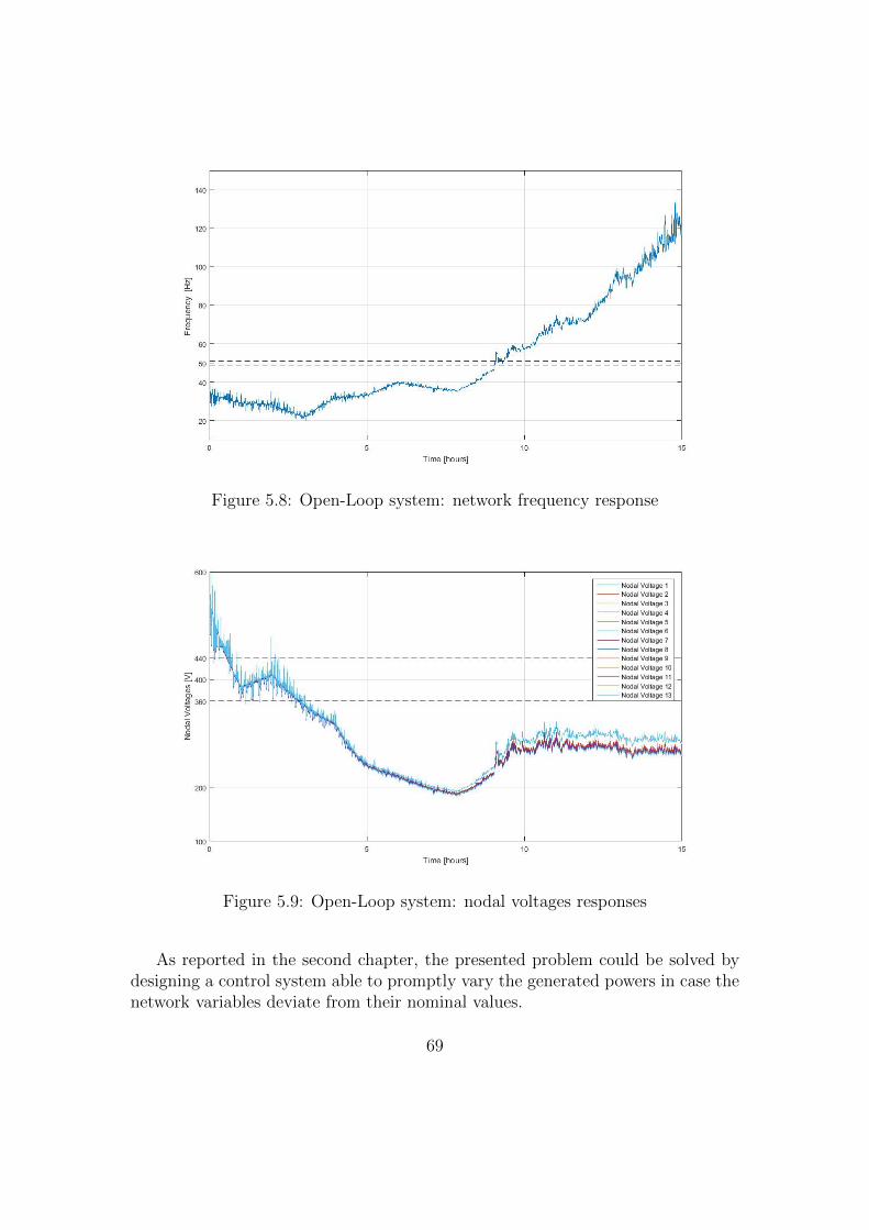
Figure 5.8: Open-Loop system: network frequency response

Figure 5.9: Open-Loop system: nodal voltages responses

As reported in the second chapter, the presented problem could be solved bydesigning a control system able to promptly vary the generated powers in case thenetwork variables deviate from their nominal values.

69

This would considerable reduce the power unbalance, eventually leading thenetwork variables to reach steady-state values not so far from their nominal values.However, another important requirement is that this control system performs afast control action since we are dealing with a low-inertia system and thereforevoltages and frequency may quickly reach steady-state values that are not allowedby the regulations. All these features can be achieved by implementing the primarycontrol layer that has been described in the second chapter. In the followingparagraph its actual implementation will be described, and also some simulationswill be performed in order to test the relative performances.

5.3.3 Primary Control: Implementation and Tests

As discussed in previous chapters, the primary control consists in two sequentialsublayers, i.e. the inverter output control and the droop control. The droopcontrol can be considered the most significant layer since it is designed to vary thegenerated powers based on the deviation of the network variables from nominalvalues. For the purpose of this work, the inverse resistive droop control approachhas been adopted. This links the variations of voltages to the variations of activepower and the variations of frequency to the variations of reactive power through aproportional control action. Being defined as a decentralized structure, this systemis located at each generation unit; its scheme is again represented in Figure 5.10.

Figure 5.10: Inverse Resistive Droop

70

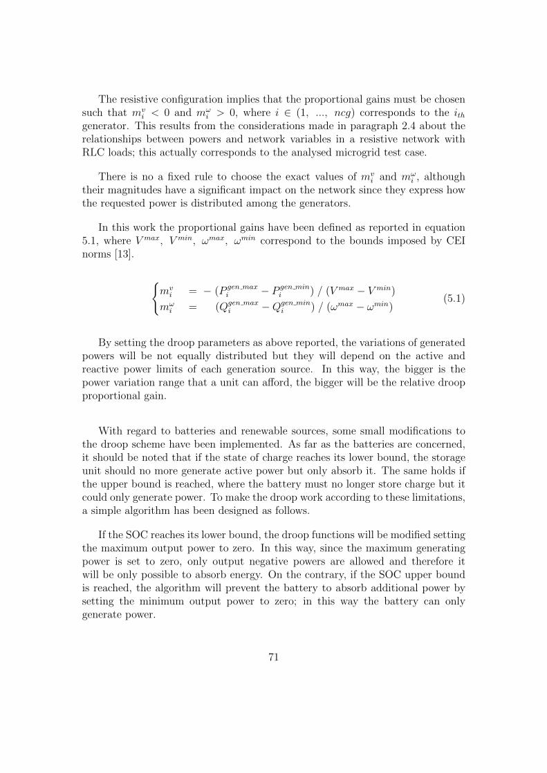
The resistive configuration implies that the proportional gains must be chosensuch that mv

i < 0 and mωi > 0, where i ∈ (1, ..., ncg) corresponds to the ith

generator. This results from the considerations made in paragraph 2.4 about therelationships between powers and network variables in a resistive network withRLC loads; this actually corresponds to the analysed microgrid test case.

There is no a fixed rule to choose the exact values of mvi and mω

i , althoughtheir magnitudes have a significant impact on the network since they express howthe requested power is distributed among the generators.

In this work the proportional gains have been defined as reported in equation5.1, where V max, V min, ωmax, ωmin correspond to the bounds imposed by CEInorms [13].

{mvi = − (P gen max

i − P gen mini ) / (V max − V min)

mωi = (Qgen max

i −Qgen mini ) / (ωmax − ωmin)

(5.1)

By setting the droop parameters as above reported, the variations of generatedpowers will be not equally distributed but they will depend on the active andreactive power limits of each generation source. In this way, the bigger is thepower variation range that a unit can afford, the bigger will be the relative droopproportional gain.

With regard to batteries and renewable sources, some small modifications tothe droop scheme have been implemented. As far as the batteries are concerned,it should be noted that if the state of charge reaches its lower bound, the storageunit should no more generate active power but only absorb it. The same holds ifthe upper bound is reached, where the battery must no longer store charge but itcould only generate power. To make the droop work according to these limitations,a simple algorithm has been designed as follows.

If the SOC reaches its lower bound, the droop functions will be modified settingthe maximum output power to zero. In this way, since the maximum generatingpower is set to zero, only output negative powers are allowed and therefore itwill be only possible to absorb energy. On the contrary, if the SOC upper boundis reached, the algorithm will prevent the battery to absorb additional power bysetting the minimum output power to zero; in this way the battery can onlygenerate power.

71

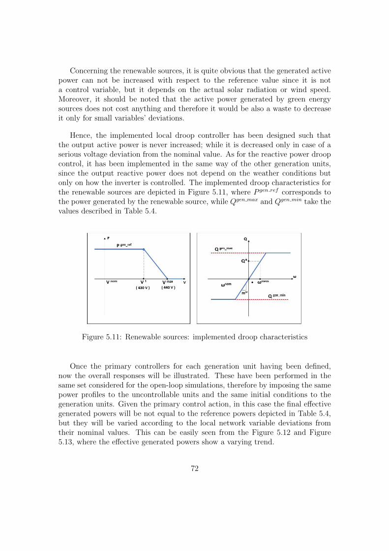
Concerning the renewable sources, it is quite obvious that the generated activepower can not be increased with respect to the reference value since it is nota control variable, but it depends on the actual solar radiation or wind speed.Moreover, it should be noted that the active power generated by green energysources does not cost anything and therefore it would be also a waste to decreaseit only for small variables’ deviations.

Hence, the implemented local droop controller has been designed such thatthe output active power is never increased; while it is decreased only in case of aserious voltage deviation from the nominal value. As for the reactive power droopcontrol, it has been implemented in the same way of the other generation units,since the output reactive power does not depend on the weather conditions butonly on how the inverter is controlled. The implemented droop characteristics forthe renewable sources are depicted in Figure 5.11, where P gen ref corresponds tothe power generated by the renewable source, while Qgen max and Qgen min take thevalues described in Table 5.4.

Figure 5.11: Renewable sources: implemented droop characteristics

Once the primary controllers for each generation unit having been defined,now the overall responses will be illustrated. These have been performed in thesame set considered for the open-loop simulations, therefore by imposing the samepower profiles to the uncontrollable units and the same initial conditions to thegeneration units. Given the primary control action, in this case the final effectivegenerated powers will be not equal to the reference powers depicted in Table 5.4,but they will be varied according to the local network variable deviations fromtheir nominal values. This can be easily seen from the Figure 5.12 and Figure5.13, where the effective generated powers show a varying trend.

72

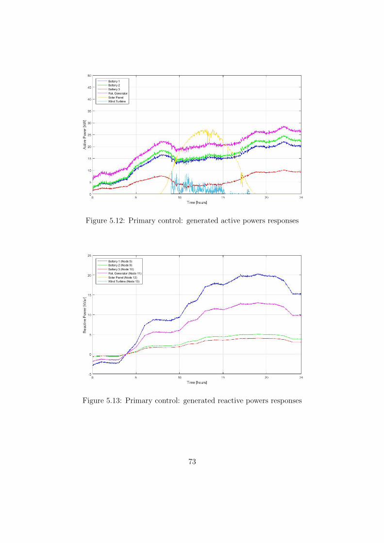
Figure 5.12: Primary control: generated active powers responses

Figure 5.13: Primary control: generated reactive powers responses

73

Although the powers are varied by simple proportional gains, the requested loadpower has been efficiently distributed among the controllable generation sources.Regarding the dispatchable units (i.e. batteries and rotating generator), the powerdistribution is obviously not equal since it depends on the droop parameters. Asabove reported, the droop control has been designed such that the more power aunit can either generate or absorb, the larger will be the relative power variation.

With regard to the network variables, by looking at Figure 5.14 and Figure5.15 it is possible to appreciate significant improvements with respect to the openloop case. Indeed, the droop scheme is able to keep the network variables aroundrealistic values, respecting for most of the time the bounds imposed by the regu-lations.

However, it can be surely noted that neither the frequency nor the voltageskeep their nominal values, which are 50 Hz and 400 V, respectively. This is morerelevant feature for the frequency, since it is recalled that, in case of a possiblereconnection with the main grid, it is strictly required that at the interconnectionthe two systems are synchronized at the same frequency. About nodal voltages, itis possible to notice that they show a decreasing behavior due since the load powersare continuously increasing over the whole day, as reported by Figure 5.6 and 5.7.It can be appreciated that the active power generated by renewable sources givesa great help since it prevents the nodal voltages to drastically exceed the lowerbound. This is witnessed by an evident increase on the nodal voltages trend overthe central hours of the day. However, once the active power from renewablesources come back to zero, the droop control is not able to keep the voltages abovethe lower bound.

Finally, in Figure 5.16 the states of charge are illustrated, showing obviouslya decreasing trend; in fact the batteries have generated power for the whole sim-ulation time. The amount of discharged energy is not equal among the differentbatteries both because they generated different values of active power and alsobecause they are characterized by different capacities and charge/discharge coeffi-cients, as previously shown in Table 5.1.

As the following figures show, although the primary controllers guarantee greatimprovements with respect to the open loop case, they are not the best solutionto manage an islanded microgrid. Pure proportional actions are in fact extremelyefficient in ensuring a fast and considerable reduction of network variable devia-tions, but they are not able to make the network variables evolve close to theirnominal values. Moreover, through this simple control structure is not possibleto implement any resource management logic, taking for example the remainingstates of charge of the batteries or some economic factors.

74

Figure 5.14: Primary Control: network frequency response

Figure 5.15: Primary Control: nodal voltages responses

75

Figure 5.16: Primary Control: batteries’ SOCs responses

There is an additional degree of freedom that this control structure is notexploiting, which corresponds to actually vary the reference active and reactivepowers according to the network conditions. In this way in fact, the steady-statedeviations can be furtherly decreased and an efficient resource power managementcan be implemented. These motivations lead to the design of a higher control layer,which actual implementation have been largely described in the fourth chapter.The numerical results of the complete hierarchical control structure will be shownin the next paragraph.

5.3.4 Hierarchical Control: Implementation and Tests

The use of a centralized secondary controller allows to ensure an efficient coordi-nation of all the controllable units, achieving the defined control objectives. Thesecondary control layer is composed of two main elements: the frequency integra-tor and the Model Predictive Controller, which have been largely discussed in theprevious chapters. Before showing the main results of the performed simulations,some considerations on the design specifications are worth to be described; theseare reported in the next paragraph.

76

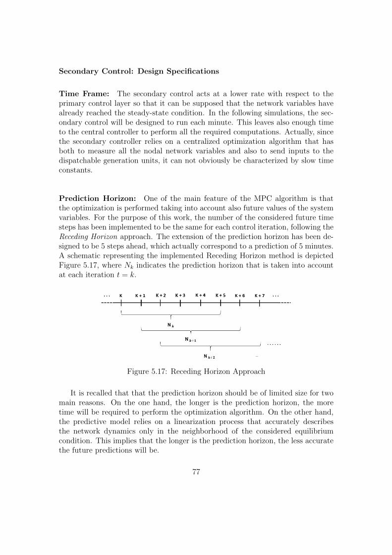
Secondary Control: Design Specifications

Time Frame: The secondary control acts at a lower rate with respect to theprimary control layer so that it can be supposed that the network variables havealready reached the steady-state condition. In the following simulations, the sec-ondary control will be designed to run each minute. This leaves also enough timeto the central controller to perform all the required computations. Actually, sincethe secondary controller relies on a centralized optimization algorithm that hasboth to measure all the nodal network variables and also to send inputs to thedispatchable generation units, it can not obviously be characterized by slow timeconstants.

Prediction Horizon: One of the main feature of the MPC algorithm is thatthe optimization is performed taking into account also future values of the systemvariables. For the purpose of this work, the number of the considered future timesteps has been implemented to be the same for each control iteration, following theReceding Horizon approach. The extension of the prediction horizon has been de-signed to be 5 steps ahead, which actually correspond to a prediction of 5 minutes.A schematic representing the implemented Receding Horizon method is depictedFigure 5.17, where Nk indicates the prediction horizon that is taken into accountat each iteration t = k.

Figure 5.17: Receding Horizon Approach

It is recalled that that the prediction horizon should be of limited size for twomain reasons. On the one hand, the longer is the prediction horizon, the moretime will be required to perform the optimization algorithm. On the other hand,the predictive model relies on a linearization process that accurately describesthe network dynamics only in the neighborhood of the considered equilibriumcondition. This implies that the longer is the prediction horizon, the less accuratethe future predictions will be.

77

Knowledge of the system: At this stage, it is supposed that the secondarycontroller has a complete knowledge of the network parameters, as well as of theunits’ characteristics. Moreover, also the predictions of the power trends of loadsand renewable sources are supposed to be available. Since it is quite difficult tohave such detailed information on the system, in the Section 5.4 a more realisticimplementation will be taken into account.

Cost Function and Constraints: Looking at the actual optimization prob-lem, the weights of the cost function have been set so that the network variables’deviations have more importance than the other system variables in the minimiza-tion process. At this stage, the optimization process does not take into accounta possible resource management strategy and therefore all the generation sourcesare equally weighted in the cost function.

Concerning the variable constraints, their implementation have been alreadydescribed in the fourth chapter, where most of them refer either to regulations’bounds or to physical limits. This does not hold for two precise constraints, whosethe corresponding bounds are design parameters. The former defines the SOCmaximum and minimum recommended bound, which have been set to be 20% and80%. Moreover, since also the control inputs corresponding to the variations ofreference powers are limited, and in the following simulations a maximum variationof ±5 kW (kVar) will be allowed.

Moreover, an additional constraint needs to be defined since the rotating gen-erator is not characterized by a pure squared capability curve but also a limitationon the minimum power factor exists (look at Figure 5.3). This means that aconstraint taking into account the ratio between the actual generated active andreactive power has been also implemented.

Hierarchical control simulations

Once all the MPC parameters have been set, the actual simulations can be per-formed. As in the previous tests, the power trends illustrated in the Figures 5.5,5.6 and 5.7 will be implemented, as well as the same initial conditions. However,it is recalled that now also the reference ones will be varied by the hierarchicalcontrol structure so that smaller voltages and frequency deviations are allowed.The final simulations’ outcomes are illustrated in the following figures.

78

Figure 5.18: Hierarchical Control: network frequency response

Figure 5.19: Hierarchical Control: nodal voltages responses

79

Figure 5.20: Hierarchical Control: generated active powers responses

Figure 5.21: Hierarchical Control: generated reactive powers responses

80

Figure 5.22: Hierarchical Control: batteries’ SOCs responses

By looking at the first two graphs, the main achievements of the designed con-trol structure can be appreciated. Actually, by performing the system simulationswith exactly the same initial conditions, it can be noticed that now the networkvariables evolve really close to their nominal values for the whole simulation time.Moreover, the microgrid frequency shows an almost null static error due to thepresence of the integrator, properly placed as described in the previous chapters.On the other hand, voltages are not exactly equal to their nominal value, but theyare kept between 390 V and 410 V. This can be considered quite satisfactory sincethe network can afford small voltage deviations without any consequence. What ismore, given the flexibility of the cost function, if a lower voltage offset was requiredit would be enough to increase the corresponding weight.

A more accurate look at the active and the reactive powers shows that a biggeramount of power is generated with respect to the previous cases. This is moreevident for the active powers, since three out of four generation sources reach theirmaximum power limits in the final part of the day, according to their parameterspreviously defined. This is because the generation powers try to equal the actualpower absorption in order to minimize the variable deviations, taking eventuallygreater values with respect to the previous simulations.

81

Remark: As far as the states of charge are concerned, it is worth noticing thatthey are kept inside the recommended bounds for most of the simulation time,apart from the battery placed at node 5, indicated as battery 1; this behavior isnot surprising according to the implemented secondary control logic. Actually,the SOC of the battery 1 reaches the lower bound at about the 16th hour. Giventhe imposed constraint, the secondary control layer modifies the correspondingactive power so that it is set to zero when the SOC reaches its lower bound, asit can be noticed from Figure 5.20 by looking at the blue trend. However, atabout the 18th hour, all the remaining generators have reached their active powerlimits, although the active load power absorption continues to increase. Since themain control objective is to keep the network variables near to the nominal values,the MPC decides to allow the battery 1 to generate the remaining load power,furtherly discharging the battery SOC. It is in fact recalled that the operationsbounds for the states of charge have been implemented as Soft Costraints, whichin some cases can be violated.

To sum up, starting from the description of the considered test case, the hier-archical control structure shows great improvements with respect to the previouscases. Indeed, although the microgrid is subject to varying and noisy power trends,the network variables never exceed the bounds imposed by the regulations and,what is more, they maintain their nominal values for the whole simulation time.Nevertheless, to test the robustness of the designed control system, in the nextsections additional simulations will be presented.

82

5.4 System Robustness Tests

In this section, the control framework will be tested in three different scenarios.Firstly, it will be supposed that the control system has a pretty limited knowledgeof the system parameters, testing if the designed control structure shows robustcharacteristics with respect to model’s uncertainties. Then, it will be shown howthe flexibility of the MPC approach allows to implement different resource man-agement logics by simply changing the cost function’s weights. Finally, a morerealistic context will be considered, testing the control structure with identifiedload models corresponding to real utilities.

5.4.1 Limited knowledge of the system

In this section, some features of the implemented MPC algorithm have been re-moved, although they could be considered feasible from a theoretical point of view.

In the previous chapters, it was supposed that the control system had a com-plete knowledge of the future power trends of the uncontrollable units, which havebeen modeled as known disturbances. Moreover, also the dependence of the loadpower with respect to the network variables was assumed to be available, beingactually inserted in the network jacobian (see paragraph 3.3). This does not repre-sent a realistic implementation since it is quite difficult to have such detailed dataon the load characteristics. Therefore, taking into account a more realistic view,in the following simulations it will be supposed that all the information about theuncontrollable sources, both related to their internal parameters and future powertrends, are not available to the central controller.

Moreover, it is unlikely the case that an exact knowledge of the line impedancesis accessible. It should be also noted that, depending on the circulating currents,the line impedances’ values can considerably grow with respect to the nominalvalues, as reported in [28]. Because of this, in the following simulations it will as-sumed that only the nominal values of line impedances are known to the controller,while the real implemented values have been increased by a 50% factor.

Obviously, introducing the above mentioned uncertainties of the real param-eters implies that the hierarchical control structure will rely on a slightly wrongsystem model and consequently the computed control actions may be not theoptimal ones to implement.

83

In the following simulations, the same initial conditions and power trends illus-trated in paragraph 5.3.1 have been implemented. The figures show that, althoughthe controller has not an exact knowledge of the system, the main control objec-tives have been achieved. It can be noticed that the voltages are slightly morenoisy and slightly more distant from their nominal value with respect to the pre-vious test. However, their trends are satisfactory since it is recalled that voltagesare not required to evolve exactly at their nominal value, but it is more relevantthat they never exceed the imposed bounds.

Finally, with regard to the generated active and reactive powers, respectivelydepicted in Figure 5.25 and Figure 5.26, it is possible to note that they do notshow such a different behavior with respect to the base case. This is due to thefact that they do not significantly depend on the knowledge that the controller hasabout the system, but their trends are more related to the uncontrollable powerprofiles and to the implemented control strategy in the cost function.

Figure 5.23: Limited System Knowledge: network frequency response

84

Figure 5.24: Limited System Knowledge: nodal voltages responses

Figure 5.25: Limited System Knowledge: generated active power responses

85

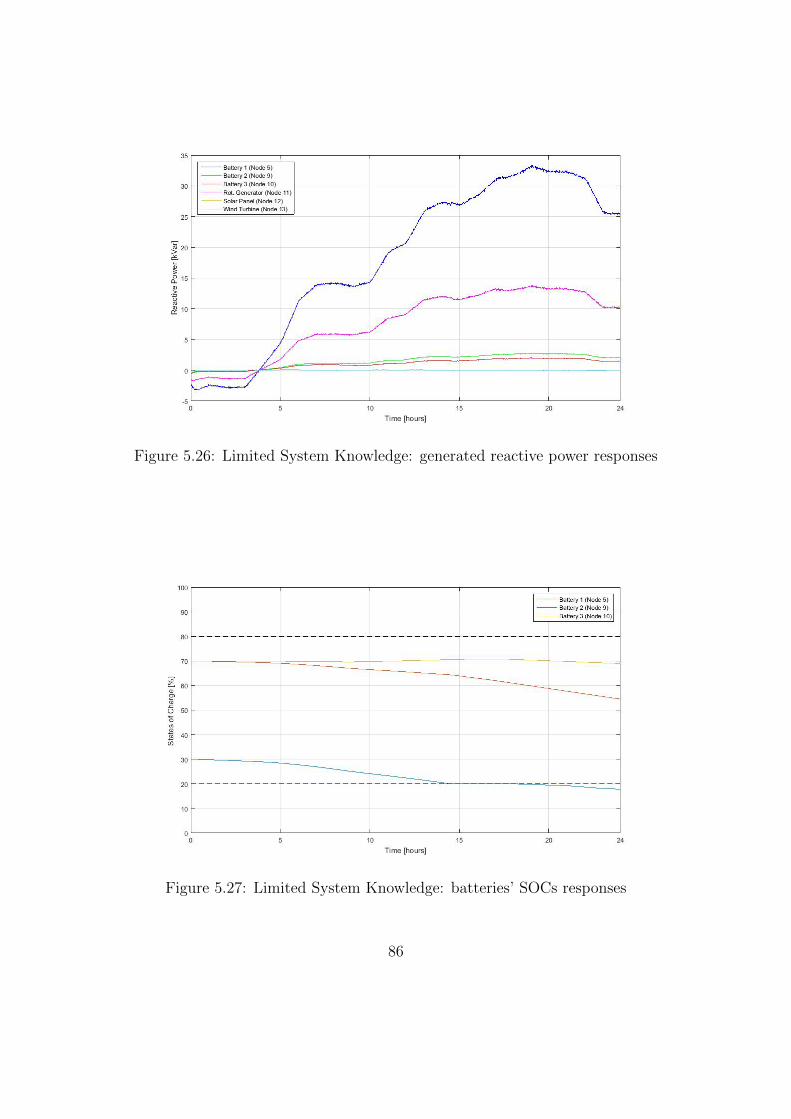
Figure 5.26: Limited System Knowledge: generated reactive power responses

Figure 5.27: Limited System Knowledge: batteries’ SOCs responses

86

The previous figures show that the developed control system is quite robustwith respect to the introduced uncertainties. Actually, although a complete knowl-edge of the system parameters was not available, the combined action of the pri-mary and secondary control layers was however able to manage the consideredmicrogrid in the islanded operating mode accomplishing the defined control objec-tives.

5.4.2 Resource Management Control Logics

At this stage, a control logic that manages the different sources according to pre-defined targets has not still implemented. Depending on the considered scenario,there could be some circumstances where it is more convenient to exploit one kindof source rather than another. To implement simple resource management strate-gies, it is enough to change the values of some weights of the defined cost function.This will be shown taking into account two possible case examples, which be pre-sented in the next paragraphs. In the following simulations, the uncontrollablepower trends previously illustrated are implemented, while the initial conditionsare set as reported in Table 5.6.

P gen ref Qgen ref SOCBattery 1 5 kW 0 kVar 50%Battery 2 5 kW 0 kVar 50%Battery 3 5 kW 0 kVar 50%Rotating Generator 5 kW 0 kVar −−

Table 5.6: Resource Management Control Logics: Initial Conditions

Moreover, considering a more realistic implementation of the defined controlstructure, the model uncertainties introduced in the previous section will be keptfor the following tests.

87

Economic Microgrid Management

There are some cases where it is better to minimize the energy provided by therotating generator and to greatly exploit the storage units and the renewablesources. For instance, if it is expected that the microgrid will operate in islandedmode only for few hours, it is not fundamental to preserve the energy stored in thebatteries for a future use, but it could more convenient to take into account someeconomic factors. Actually, differently from batteries, the energy provided by therotating generator has a significant cost since it is based on a fuel combustionprocess.

A simply way to implement the corresponding control logic corresponds tomodify cost functions parameters such that the active power provided by batteriesis considerably less weighted with respect to the one generated by the rotatingsource. Implementing that case, the responses of the main variables are illustratedin the following figures.

Figure 5.28: Economic Microgrid Management: network frequency response

88

Figure 5.29: Economic Microgrid Management: nodal voltages responses

Figure 5.30: Economic Microgrid Management: generated active power responses

89

Figure 5.31: Economic Microgrid Management: generated reactive power re-sponses

Figure 5.32: Economic Microgrid Management: batteries’ SOCs responses

90

The figures show that it has been possible to implement a “cheaper” resourcemanagement strategy, without affecting the network system variables. Actually,the frequency is always kept at its nominal value while the voltages continue toevolve pretty far from the bounds imposed by the regulations. By comparing theFigure 5.30 and Figure 5.25, it is possible to notice that in this case the rotatinggenerator delivers a considerably smaller amount of energy with respect to theprevious cases. It in fact reaches a peak of 33 kW only in the final part of the daywhere it is recalled that the power absorption significantly increases.

Remark: Looking at Figure 5.30, it can be noticed that during the central partof the day the battery 3 absorbs energy, taking negative values of output power,while the rotating generator is generating an active power between 10 kW and 15kW. This could seem a counter-intuitive behavior since it was reported that theimplemented resource management strategy minimizes the energy delivered by thecombustion-based generator and tries to make only the storage units generate theneeded power. Looking at Figure 5.2, it can be also noted that the battery 3, whichis located at node 10, is the closest storage unit to renewable sources, placed atnode 12 and 13, respectively. Moreover, when the renewable sources start to gen-erate, since their active powers are not regulated by primary controllers in normalconditions, the corresponding nodal voltages increase. Since the designed maincontrol objective remains to keep the network variables near their nominal values,it happens that the MPC controller considerably decreases the reference power ofthe battery 3 such that it absorb as much energy as possible by the green energysources. In this way, the battery compensates the power unbalances caused byrenewable generators, and consequently the network variables do not considerablydeviate from their nominal values. To sum up, although resource managementstrategies can be implemented, the control structure is designed such that theminimization of the network variables’ deviations is always the first priority.

Robust Microgrid Management

There are others cases where it could be more relevant to preserve the batteries’charge and it is more reliable to make the rotating generator produces a consider-ably amount of active power. For instance, if the microgrid is supposed to operatein the islanded condition for a long time, which could be unknown a priori, it isnot recommended to consume all the batteries’ power, but it could be more safeto sustain the microgrid with fully dispatchable generators. This simply resourcemanagement strategy can be implemented by changing the cost functions param-eters such that the active powers produced by batteries are more weighted withrespect to the rotating generator one.

91

With same simulation specifications of the previous section, the main variableresponses follow.

Figure 5.33: Robust Microgrid Management: network Frequency response

Figure 5.34: Robust Microgrid Management: nodal voltages responses

92

Figure 5.35: Robust Microgrid Management: generated active power responses

Figure 5.36: Robust Microgrid Management: generated reactive power responses

93

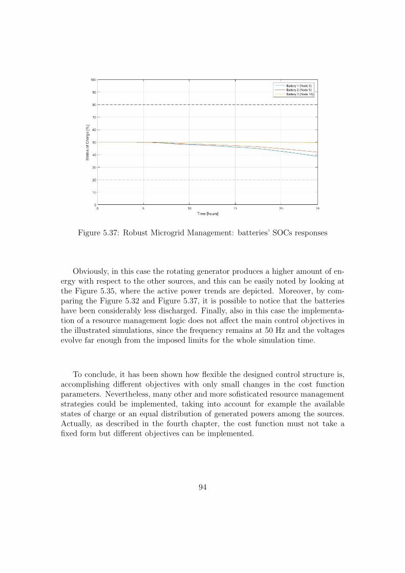
Figure 5.37: Robust Microgrid Management: batteries’ SOCs responses

Obviously, in this case the rotating generator produces a higher amount of en-ergy with respect to the other sources, and this can be easily noted by looking atthe Figure 5.35, where the active power trends are depicted. Moreover, by com-paring the Figure 5.32 and Figure 5.37, it is possible to notice that the batterieshave been considerably less discharged. Finally, also in this case the implementa-tion of a resource management logic does not affect the main control objectives inthe illustrated simulations, since the frequency remains at 50 Hz and the voltagesevolve far enough from the imposed limits for the whole simulation time.

To conclude, it has been shown how flexible the designed control structure is,accomplishing different objectives with only small changes in the cost functionparameters. Nevertheless, many other and more sofisticated resource managementstrategies could be implemented, taking into account for example the availablestates of charge or an equal distribution of generated powers among the sources.Actually, as described in the fourth chapter, the cost function must not take afixed form but different objectives can be implemented.

94

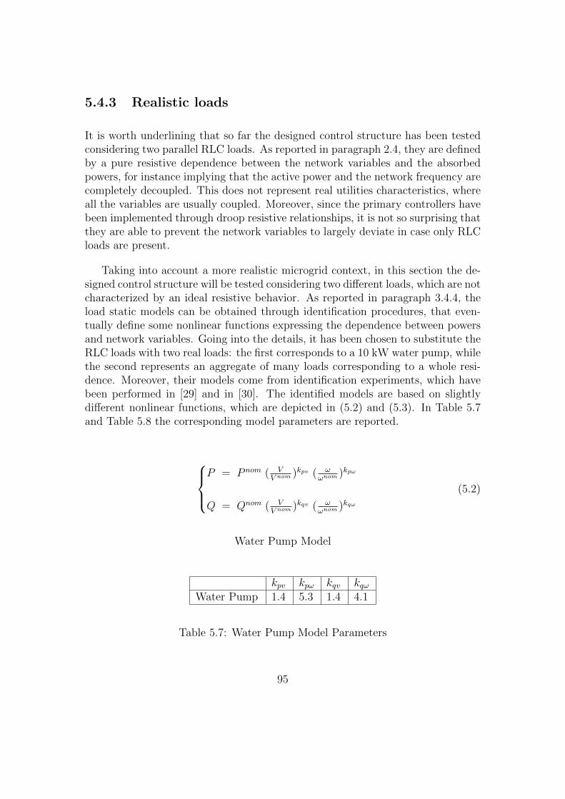
5.4.3 Realistic loads

It is worth underlining that so far the designed control structure has been testedconsidering two parallel RLC loads. As reported in paragraph 2.4, they are definedby a pure resistive dependence between the network variables and the absorbedpowers, for instance implying that the active power and the network frequency arecompletely decoupled. This does not represent real utilities characteristics, whereall the variables are usually coupled. Moreover, since the primary controllers havebeen implemented through droop resistive relationships, it is not so surprising thatthey are able to prevent the network variables to largely deviate in case only RLCloads are present.

Taking into account a more realistic microgrid context, in this section the de-signed control structure will be tested considering two different loads, which are notcharacterized by an ideal resistive behavior. As reported in paragraph 3.4.4, theload static models can be obtained through identification procedures, that even-tually define some nonlinear functions expressing the dependence between powersand network variables. Going into the details, it has been chosen to substitute theRLC loads with two real loads: the first corresponds to a 10 kW water pump, whilethe second represents an aggregate of many loads corresponding to a whole resi-dence. Moreover, their models come from identification experiments, which havebeen performed in [29] and in [30]. The identified models are based on slightlydifferent nonlinear functions, which are depicted in (5.2) and (5.3). In Table 5.7and Table 5.8 the corresponding model parameters are reported.

P = P nom ( V

V nom )kpv ( ωωnom )kpω

Q = Qnom ( VV nom )kqv ( ω

ωnom )kqω(5.2)

Water Pump Model

kpv kpω kqv kqωWater Pump 1.4 5.3 1.4 4.1

Table 5.7: Water Pump Model Parameters

95

P = P nom ( V

V nom )kpv (1 + kpω(ω − ωnom))

Q = Qnom ( VV nom )kqv (1 + kqω(ω − ωnom))

(5.3)

Residential Model

kpv kpω kqv kqωResidential Load 1.2 0.7 2.7 -2.3

Table 5.8: Residential Model Parameters

Looking at these loads, it can be noted that they are not characterized by pureresistive relationships but all variables are correlated. It is in fact recalled thatthe parameters shown in the tables express how one variable is correlated to theother. This is more relevant for the water pump, where a significant dependencebetween the active power and the network frequency is present (the parameter kpωhas in fact a bigger value with respect to the others). This is due to the fact thatthe water pump is a rotating load, which is usually characterized by an inductiverelationship.

Having defined the load characteristics, their nominal power trends are nowillustrated. At this stage, two different profiles are defined for each load: oneprofile will represent the active power trend, while the other shows how the powerfactor evolves during the whole simulation time. Actually, real loads are nevercharacterized by two independent active and a reactive power profiles, as performedin the previous simulations, but their power factor is usually varied. However, itis recalled that given the active power and the power factor, the resulting reactivepower can be easily computed by performing the following computation.

Q = P tan ( acos( cos(φ) ) )

The implemented load profiles are illustrated in Figures 5.33 and 5.34.

96

Figure 5.38: Realistic Loads: Power Factor Profile

Figure 5.39: Realistic Loads: Active Power Profile

With regard to initial conditions of the generation sources, the data depictedin Table 5.6 have been implemented, while the renewable sources follow the same

97

power trends of the previous simulations. Moreover, also in this case the samescenario considered in paragraph 5.4.1 has been assumed, taking into account amore realistic test. The main results of the implemented simulation are depictedin the following figures.

Figure 5.40: Robust Microgrid Management: network frequency response

Figure 5.41: Realistic Loads: nodal voltages responses

98

Figure 5.42: Realistic Loads: generated active power responses

Figure 5.43: Realistic Loads: generated reactive power responses

99

Figure 5.44: Realistic Loads: batteries’ SOCs responses

The figures show that also in this case the control objectives are achieved. Tosum up, in this simulation the control system does not have information aboutload power forecasts and on the load characteristics. Moreover, the implementedloads are not described by pure resistive relationships.

It has to be noted that from the simulated case it is not possible to conclude thedesigned hierarchical control structure perfectly works in any microgrid context.Actually, as discussed in the second chapter, to design the primary control layer it isreally important to understand which is the prevailing impedance of the microgrid.Obviously, if the microgrid was characterized by inductive lines and only rotatingloads were implemented, the designed control structure would be not able to keepthe network variables at their nominal values. However, two facts are worth to beunderlined.

Firstly, in the future most microgrids will be characterized by a resistive pre-vailing impedance. Indeed they are characterized by short resistive lines and itwill be really unusual to find rotating loads directly connected to lines. Giventhe recent developments in power electronics converters, it will be more and morecommon that all microgrid elements are interfaced with electronically-controlledinverters instead of being directly plugged into the network.

100

On the other hand, it can be also noted that the defined control structure is notdependent on the implemented droop relationship. Actually, the inductive inversedroop control can be easily adopted without changing the secondary controller, butonly by updating the system model used to perform the optimization algorithm.Therefore, in case we are dealing with a microgrid that shows a prevailing inductiverelationship, the hierarchical control approach can be all the same implemented,achieving the defined control objectives.

5.5 Conclusions

In this chapter the microgrid test case has been presented and the performancesof the designed control structure have been discussed. Summarizing, it has beenproved that the implementation of a predictive secondary control layer gives con-siderable improvements since the network variables do not significantly deviatefrom their nominal values. Moreover, it allows to implement different policiesfor the resource management according to predefined objectives. It has been alsoshown that the hierarchical control structure is not strictly dependent on the exactknowledge of the system.

101

Chapter 6

Conclusions and FutureDevelopments

In the first chapter, a complete overview of the future microgrid context has beenpresented, describing the main issues involving this new electrical paradigm. Theseare more relevant in the so called islanded operating mode, where frequent unbal-ances between the total generated and requested power occur. Actually, as shownin the second chapter, these unbalances significantly affect the network voltagesand frequency, making them deviate from their nominal values. To solve this prob-lem, in the same chapter a primary decentralized control layer has been described,analyzing both its theoretical definition and the adopted configuration. However,in the final part of the second chapter it is reported that this control layer is notenough to ensure that the network variables evolve around their nominal values.

Therefore, the implementation of a higher control layer has been considered,which actually corresponds to the main innovation introduced by this work. Thissecondary control layer has been chosen to be based on an advanced control strat-egy, i.e. the Model Predictive Control. Actually, the corresponding flexibilityand potentialities make this control approach an efficient solution to the men-tioned problems, allowing also the implementation of different resource manage-ment strategies during the islanded operating mode. However, since this controlapproach relies on a mathematical model of the system, the third chapter focusedon the analysis of the main system dynamics. Once the final state-space equationdescribing the behavior of the main variables of the microgrid has been defined,in the final part of the chapter a description of the network simulator has beengiven, which has been developed by RSE SpA.

102

The fourth chapter covered the designing of the secondary control layer, an-alyzing its main elements. It is recalled that Model Predictive Control is basedon an online optimization algorithm which relies on three principal elements: thesystem model, the variables’ constraints and the cost function. While the first hasbeen largely described in the third chapter, the implemented constraints and costfunction have been presented in this chapter. However, given the flexibility of thisadvanced control technique, it is recalled that the designed control objectives canbeen easily extended or modified.

Finally, in the fifth chapter the designed hierarchical control structure has beentested. In the first part, the considered microgrid test case and its main elementshave been described, which actually correspond to a real small-scale network thatRSE owns at their main headquarters. Then, a series of simulations have beenreported and it has been shown how the designed control structure is able toefficiently manage the considered microgrid in the islanded mode.

At the end of the chapter, additional tests have been presented where a morerealistic implementation has been taken into account, for instance limiting theknowledge that the controller has on the system parameters or by testing thedesigned control structure with real utilities instead of simple RLC loads. Fur-thermore, it has been also proved that the flexibility of designed control structureallows to implement different resource management strategies without affectingthe network variables’ stabilization.

Considering the proposed solution, the main advantages of implementing thesecondary control layer with a predictive control approach can be underlined:

• Coordinating all the primary controllers of the microgrid sources, this allowsto keep the network variables at their nominal values in each power condition.

• Its flexibility allows to easily implement different resource management strate-gies without varying the designed control structure, but only by changingsome parameters.

• It can perform an efficient microgrid management by taking into accountsome forecasts about the renewable sources production and load power futuretrends, if available.

Although the results of the designed control structure are satisfying, there aremany other aspects that would be worth investigating through additional researchactivities; some of them are now presented.

103

• The implemented optimization algorithm takes into account only the mini-mization of the generated output powers for the resource management. How-ever, more complex control strategies could be implemented. For instance,it could be interesting to control the generator reference powers based ontheir distance from the power limits, rewarding the units that allow biggerregulation margins. Another relevant resource management strategy couldtake into account the units’ efficiency, trying to minimize the resource con-sumption in terms of batteries’ states of charge or consumed fuel of thecombustion-based generators.

• Analyzing the implemented primary layer, it can be noted that there is anadditional degree of freedom that has been not exploited. Actually, thedroop functions are characterized by fixed slopes and only their referencepowers are varied. A more complex hierarchical control structure could beimplemented, which can consist in more than two layers, and that is able tovary both the reference powers and the droop proportional gains accordingto some predefined objectives.

• The actual control structure is characterized by a centralized secondary con-troller that coordinates all the generation sources. However, this approachimplies that a high computational power is required. Moreover, if a newmicrogrid element is plugged into the network or a unit is disconnected,this centralized control structure needs to be reformulated with a new sys-tem model. To overcome this issue, it would be interesting to investigatethe possibility of implementing a decentralized secondary control layer thatit is however based on an optimization based control algorithm, such as adistributed Model Predictive Control. This would allow in fact a flexiblecontrol framework, which all the same ensures an efficient management ofthe microgrid elements.

• Finally, the proposed control system has been designed to manage the micro-grid only in islanded condition, and it does not consider neither the islandingnor the reconnecting event. The hierachical control structure could be actu-ally improved so that it is performed both in islanded and in grid-connectedmode, ensuring an efficient energy management in both conditions. More-over, it has to be noted that an accurate analysis of the network variablestransients should be performed during both the islanding and the recconnect-ing event; they may in fact experience unstable behaviors if the generationsources are not properly controlled.

104

List of Figures

1.1 Microgrid general structure . . . . . . . . . . . . . . . . . . . . . . 51.2 Inductive droop characteristics . . . . . . . . . . . . . . . . . . . . . 81.3 Hierarchical control structure . . . . . . . . . . . . . . . . . . . . . 91.4 Proposed control scheme . . . . . . . . . . . . . . . . . . . . . . . . 11

2.1 Inverter simplified circuit . . . . . . . . . . . . . . . . . . . . . . . . 152.2 Simple electrical network . . . . . . . . . . . . . . . . . . . . . . . . 172.3 Phasor representation of nodal voltages . . . . . . . . . . . . . . . . 182.4 Conventional Resistive Droop . . . . . . . . . . . . . . . . . . . . . 212.5 Inverse Resistive Droop . . . . . . . . . . . . . . . . . . . . . . . . . 222.6 Implemented droop characteristics . . . . . . . . . . . . . . . . . . . 232.7 Simple network . . . . . . . . . . . . . . . . . . . . . . . . . . . . . 24

3.1 Time Discretization . . . . . . . . . . . . . . . . . . . . . . . . . . . 273.2 Hierarchical control block diagram . . . . . . . . . . . . . . . . . . 283.3 Nodal Power Balance . . . . . . . . . . . . . . . . . . . . . . . . . 303.4 Frequency Integrator . . . . . . . . . . . . . . . . . . . . . . . . . . 363.5 Time Discretization (SOC) . . . . . . . . . . . . . . . . . . . . . . . 38

4.1 Hierarchical control block diagram . . . . . . . . . . . . . . . . . . 45

5.1 RSE Test Facility . . . . . . . . . . . . . . . . . . . . . . . . . . . . 585.2 Test Facility Schematic . . . . . . . . . . . . . . . . . . . . . . . . . 595.3 Rotating Generator Capability Region . . . . . . . . . . . . . . . . 625.4 Trasmission Line π-model . . . . . . . . . . . . . . . . . . . . . . . 645.5 Renewable Energy Sources: Power Profiles . . . . . . . . . . . . . . 655.6 RLC Loads: Active Power Profiles . . . . . . . . . . . . . . . . . . . 665.7 RLC Loads: Reactive Power Profiles . . . . . . . . . . . . . . . . . 675.8 Open-Loop system: network frequency response . . . . . . . . . . . 695.9 Open-Loop system: nodal voltages responses . . . . . . . . . . . . . 695.10 Inverse Resistive Droop . . . . . . . . . . . . . . . . . . . . . . . . . 705.11 Renewable sources: implemented droop characteristics . . . . . . . 72

105

5.12 Primary control: generated active powers responses . . . . . . . . . 735.13 Primary control: generated reactive powers responses . . . . . . . . 735.14 Primary Control: network frequency response . . . . . . . . . . . . 755.15 Primary Control: nodal voltages responses . . . . . . . . . . . . . . 755.16 Primary Control: batteries’ SOCs responses . . . . . . . . . . . . . 765.17 Receding Horizon Approach . . . . . . . . . . . . . . . . . . . . . . 775.18 Hierarchical Control: network frequency response . . . . . . . . . . 795.19 Hierarchical Control: nodal voltages responses . . . . . . . . . . . . 795.20 Hierarchical Control: generated active powers responses . . . . . . . 805.21 Hierarchical Control: generated reactive powers responses . . . . . . 805.22 Hierarchical Control: batteries’ SOCs responses . . . . . . . . . . . 815.23 Limited System Knowledge: network frequency response . . . . . . 845.24 Limited System Knowledge: nodal voltages responses . . . . . . . . 855.25 Limited System Knowledge: generated active power responses . . . 855.26 Limited System Knowledge: generated reactive power responses . . 865.27 Limited System Knowledge: batteries’ SOCs responses . . . . . . . 865.28 Economic Microgrid Management: network frequency response . . . 885.29 Economic Microgrid Management: nodal voltages responses . . . . 895.30 Economic Microgrid Management: generated active power responses 895.31 Economic Microgrid Management: generated reactive power responses 905.32 Economic Microgrid Management: batteries’ SOCs responses . . . . 905.33 Robust Microgrid Management: network Frequency response . . . . 925.34 Robust Microgrid Management: nodal voltages responses . . . . . . 925.35 Robust Microgrid Management: generated active power responses . 935.36 Robust Microgrid Management: generated reactive power responses 935.37 Robust Microgrid Management: batteries’ SOCs responses . . . . . 945.38 Realistic Loads: Power Factor Profile . . . . . . . . . . . . . . . . . 975.39 Realistic Loads: Active Power Profile . . . . . . . . . . . . . . . . . 975.40 Robust Microgrid Management: network frequency response . . . . 985.41 Realistic Loads: nodal voltages responses . . . . . . . . . . . . . . . 985.42 Realistic Loads: generated active power responses . . . . . . . . . . 995.43 Realistic Loads: generated reactive power responses . . . . . . . . . 995.44 Realistic Loads: batteries’ SOCs responses . . . . . . . . . . . . . . 100

106

List of Tables

5.1 Batteries Parameters . . . . . . . . . . . . . . . . . . . . . . . . . . 605.2 Auxiliary Cooling Systems for Batteries . . . . . . . . . . . . . . . . 615.3 Rotating Generator Parameters . . . . . . . . . . . . . . . . . . . . 625.4 Renewable Sources Power Limits . . . . . . . . . . . . . . . . . . . 635.5 Initial Conditions . . . . . . . . . . . . . . . . . . . . . . . . . . . . 685.6 Resource Management Control Logics: Initial Conditions . . . . . . 875.7 Water Pump Model Parameters . . . . . . . . . . . . . . . . . . . . 955.8 Residential Model Parameters . . . . . . . . . . . . . . . . . . . . . 96

107

Bibliography

[1] K. De Brabandere, B. Bolsens, J. Van den Keybus, A. Woyte, J. Driesen,R. Belmans. “A Voltage and Frequency Droop Control Method for ParallelImverters”. IEEE Transaction on Power Electronics, 22(4): 1107-1115, 2007.

[2] Y. Wei Li, Ching-Nan Kao. “An Accurate Power Control Strategy for Power-Electronics-Interfaced Distributed Generations Univs Operating in a Low-Voltage Multibus Microgrid”. IEEE Transaction on Power Electronics, 24(12):2977-2988, 2009.

[3] D. Wu, J. M. Guerrero, J. C. Vasquez, T. Dragicevic, F. Tang. “CoordinatedPower Control Strategy based on Primary-Frequency-Signaling for Islanded Mi-crogrids”. Industrial Electronics Society, IECON 2013 - 39th Annual Confer-ence of the IEEE

[4] T.L. Vandoorn, J.D.M. De Kooning, B. Meersman, L. Vandevelde. “Review ofprimary control strategies for islanded microgrids with power-electronic inter-faces”. Renewable and Sustainable Energy Reviews 19: 613–628, 2013.

[5] J. W. Simpson-Porco, F. Dorfler, Francesco Bullo. “Synchronous and PowerSharing for Droop-Controlled Inverters in Islanded Microgrids”. Automatica,49(9): 2603-2611, 2013.

[6] H. Bouattour, J. W. Simpson-Porco, F. Dorfler, Francesco Bullo. “Further Re-sults on Distributed Secondary Control in Microgrids”. 52nd IEEE Conferenceon Decision and Control. December 10-13, 2013. Florence, Italy.

[7] A. Bidram, F. L. Lewis, A. Davoudi. “Distributed Control in Systems for Small-Scale Power Networks: Using Multiagent Cooperative Control Theory”. IEEETransaction on Control Systems, 34(6): 56-77, 2014.

[8] D. Wu, T. Dragicevic, J. C. Vasquez, J. M. Guerrero, Y. Guan. “SecondaryCoordinated Control of Islanded Microgrids Based on Consensus Algorithms”.IEEE Energy Conversion Congress and Exposition (ECCE). September 14-18,2014. Pittsburgh, PA.

108

[9] J. A. Pecas Lopes, C. L. Moreira, A.G. Madureira. “Defining Control Strategiesfor MicroGrids Islanded Operation”. IEEE Transaction on Power Electronics,21(2): 916-924, 2006.

[10] J. M. Guerrero, J. C. Vasquez, J. Matas, L. Garcıa de Vicuna, M. Castilla.“Hierarchical Control of Droop-Controlled AC and DC Microgrids - A GeneralApproach Toward Standardization”. IEEE Transaction on Industrial Electron-ics, 58(1): 158-172, 2011.

[11] P. Bolzern, R. Scattolini, N. Schiavoni. “Fondamenti di Controlli Automatici”.McGraw-Hill Press, 2008.

[12] CEI. Norm CEI 021, “Regola tecnica di riferimento per la connessione diUtenti attivi e passivi alle reti BT delle imprese distributrici di energia elet-trica”.

[13] CEI. Norm EN 50160, “Caratteristiche della tensione fornita dalle reti pub-bliche di distribuzione dell’energia elettrica”.

[14] N. Mohan, T. M. Undeland, W. P. Robbins. “Power Electronics, Third Edi-tion”. John Wiley Press, 2003.

[15] J. Rocabert, A. Luna, F. Bllbjerg, P. Rodriguez. “Control Power Convertersin AC Microgrids”. IEEE Transaction of Power Electronics, 27(11): 4734-4749,2012.

[16] C. A. Gross, T. A. Roppel. “Fundamental of Electrical Engineering”. CRCPress, 2012.

[17] A. Timbus, M. Liserre, R. Teodorescu, P. Rodrigues, F. Bllabjerg. “Evalu-ation of current controllers for distributed power generation systems”. IEEETransaction of Power Electronics, 24(3): 654-664, 2009.

[18] K. D. Brabandere. “Voltage and Frequency Droop control in low voltagegrids by distributed generators with inverter front-end”. PhD Final Thesis,Katholieke Universiteit Leuven. October 2006.

[19] R. E. Thomas, A. J. Rosa, G. J. Toussaint. The Analysis and Design of LinearCircuits, 7th Edition”. Wiley Press, 2012.

[20] A. Villa, F. Belloni, C. Gandolfi. “Caratterizzazione sperimentale del compor-tamento di una porzione della Test Facility durante il funzionamento in isolaelettrica e studio delle interazioni tra generatori statici con controllo droop inisola”. RSE Report, February 2014.

109

[21] D. P. Kothari, I. J. Nagrath. “Modern Power System Analysis, 3rd Edition”.McGraw-Hill Press, 2003.

[22] S. Raimondi Cominesi, M. Farina, L. Giulioni, B. Picasso, R. Scattolini. “Two-layer predictive control of a micro-grid including stochastic energy sources”.American Control Conference (ACC), Chicago 2015.

[23] C. Carlini, C. Michelangeli, M. Rossi, D. Moneta, P. Mora. “Evoluzione dellereti MT attive: algoritmi di controllo centralizzato e test in campo reale”. RSEReport, January 2013.

[24] D. V. Griffiths, I. M. Smith. “Numerical Methods for Engineers, 2nd Edition”.Chapman & Hall Press, 2006.

[25] L. Magni, R. Scattolini. “Advanced and Multivariable Control”. Pitagora Ed-itrice Bologna, 2014.

[26] J.M. Maciejowski. “Predictive Control with Constraints, 1st Edition”. Pren-tice Hall Press, 2000.

[27] E. F. Camacho, C. B. Alba. “Model Predictive Control, 2nd Edition”. SpringerPress, 2007.

[28] M. Bockarjova, G. Andersson. “Transmission Line Conductor TemperatureImpact on State Estimation Accuracy”. Power Tech Conference, 2007 IEEELausanne.

[29] R. Marconato “Electrical Power Systems, Volume 1 - Second Edition”. CEI-Italian Electrotechnical Committee, 2002.

[30] “Load representation for dynamic performance analysis of power systems”.IEEE Transactions on Power Systems, 8(2): 472 - 482, 1993.

110

Ringraziamenti

Non e facile concentrare in una sola pagina a chi devo il conseguimento di questotraguardo. Esso e stato infatti frutto di impegno e sacrifici, ma sicuramente il grazieprincipale va alle persone che mi hanno accompagnato durante questo percorso.

Ringrazio innanzitutto il Professor Scattolini, il quale con grande dedizione eimpegno mi ha seguito in questo lavoro di tesi; la sua professionalita e sicurezzarimarranno sempre fonte di ammirazione. Lo ringrazio inoltre per il sostegno e lafiducia mostrata non solo per questo lavoro, ma anche per le esperienze future chemi aspetteranno.

Un particolare grazie va al Dr. Stefano Raimondi Cominesi, il quale e statofonte di continuo sostegno e aiuto per il completamento di questo lavoro. Egli sie rivelato inoltre una preziosa fonte di consiglio, indispensabile nei momenti piudifficili di questo percorso.

Un doveroso grazie va RSE S.p.A., e in particolare all’ Ing. Carlo Sandroni, perl’attenzione e gli importanti consigli che hanno permesso il compimento di questolavoro. Ringrazio anche il Prof. Carlo Novara, che con grande disponibilita mi haseguito dal Politecnico di Torino durante questi mesi di lavoro.

Un immenso grazie va sicuramente alla mia famiglia, alla quale questo lavoro ededicato. Ringrazio soprattutto i miei genitori per il sostegno e fiducia che hannosempre mostrato verso me e mia sorella per ogni nostra scelta; credo che a lorodobbiamo ogni nostro traguardo.

Ringrazio inoltre Nina, che ormai da piu di sei anni riempe la mia vita. Il suocontinuo incoraggiamento e amore sono stati fondamentali in questi ultimi 5 anni,permettendomi di affrontare qualunque difficolta e di perseguire i miei piu innatisogni.

Ringrazio infinitamente i miei piu grandi amici, in particolare Anastasia, Alessan-dra, Marco, Vincenzo, Eugenio, Guido, Peppe e Salvo, con i quali ho condivisomomenti di grande gioia e spensieratezza. Sono convinto che uno dei piu grandisuccessi sia avere persone come loro al mio fianco.

Infine, ma non per importanza, ringrazio Enrico, Fabio, Caterina, Marcella,Mattia e Luca, con i quali abbiamo condiviso ogni difficolta e vittoria, e che hannoreso questi 5 anni di universita molto piu belli di quanto si possa immaginare.