improving the protein identification performance in high
TRANSCRIPT

Improving the ProteinIdentification Performance in
High-Resolution MassSpectrometry Data
DIPLOMARBEIT
zur Erlangung des akademischen Grades
Diplom-Ingenieur
im Rahmen des Studiums
Computational Intelligence
eingereicht von
Frederico DusbergerMatrikelnummer 0725856
an derFakultät für Informatik der Technischen Universität Wien
Betreuung: Univ.-Prof. Dipl.-Ing. Dr.techn. Günther RaidlMitwirkung: Karl Mechtler
Dr. Peter Pichler
Wien, 08.10.2012(Unterschrift Verfasser) (Unterschrift Betreuung)
Technische Universität WienA-1040 Wien � Karlsplatz 13 � Tel. +43-1-58801-0 � www.tuwien.ac.at

Improving the ProteinIdentification Performance in
High-Resolution MassSpectrometry Data
MASTER’S THESIS
submitted in partial fulfillment of the requirements for the degree of
Diplom-Ingenieur
in
Computational Intelligence
by
Frederico DusbergerRegistration Number 0725856
to the Faculty of Informaticsat the Vienna University of Technology
Advisor: Univ.-Prof. Dipl.-Ing. Dr.techn. Günther RaidlAssistance: Karl Mechtler
Dr. Peter Pichler
Vienna, 08.10.2012(Signature of Author) (Signature of Advisor)
Technische Universität WienA-1040 Wien � Karlsplatz 13 � Tel. +43-1-58801-0 � www.tuwien.ac.at


Erklärung zur Verfassung der Arbeit
Frederico DusbergerSchönbrunner Straße 236/24, 1120 Wien
Hiermit erkläre ich, dass ich diese Arbeit selbständig verfasst habe, dass ich die verwende-ten Quellen und Hilfsmittel vollständig angegeben habe und dass ich die Stellen der Arbeit -einschließlich Tabellen, Karten und Abbildungen -, die anderen Werken oder dem Internet imWortlaut oder dem Sinn nach entnommen sind, auf jeden Fall unter Angabe der Quelle als Ent-lehnung kenntlich gemacht habe.
(Ort, Datum) (Unterschrift Verfasser)
i


Acknowledgements
I would like to thank my supervisors Günther Raidl from the Vienna University of Technologyas well as Karl Mechtler and Peter Pichler from the Protein Chemistry Facility at the ViennaResearch Institute of Pathology (IMP) who offered me the opportunity to work on this interestingproject.
Furthermore, I am also grateful to all my colleagues at the Protein Chemistry Facility whowere always helpful, encouraging and open for interesting discussions providing a productiveworking atmosphere. Especially, I want to thank Peter Pichler, Werner Straube and Thomas Tausfor their continuous interest in my work and their critical advice and guidance.
Finally, I would like to express my gratitude to my parents Rolf and Maria Dusberger, aswell as my partner Andreea Constantinescu for their constant moral support and confidence inme and my abilities during this work and my entire life.
This project would not have been possible without the help and support of any of the afore-mentioned persons.
iii


Abstract
The field of proteomics is concerned with the study of structure and function of proteins. Themost commonly used approach for the analysis of proteins is the bottom-up analysis where aprotein is first digested into smaller peptides which are then analyzed by LC-MS/MS in orderto confirm the identity of the original protein. To analyze these peptides they are first separatedvia liquid chromatography (LC) before their mass-over-charge ratios are recorded in the massspectrometer as MS1-spectra. Selected peptides (precursors) are fragmented yielding MS2-spectra of their respective fragment ions (MS/MS). These high-throughput experiments generatevast amounts of data and are referred to as shotgun proteomics experiments.
For the large amount of raw data an appropriate data analysis is required in order to extractas much useful information as possible and filter out superfluous and redundant parts. How-ever, common database search engines, which are used for identification of the peptides usingtheir masses and the associated MS2-spectra, currently throw away most of the information con-tained in MS2-spectra. Moreover, the benefit of the high mass-accuracy provided by state ofthe art mass spectrometers is forfeited by the instruments themselves, as the MS2-spectra of thepeptides are usually not recorded at the optimal time point where the intensity of the specificpeptide is highest. To compensate for these drawbacks sophisticated methods are necessary thatcan preprocess the spectra accordingly.
In this thesis we studied the application of two ways of MS2-spectrum preprocessing toincrease the number of spectra that can be identified by facilitating the identification step of thedatabase search engine.First, different MS2-deisotoping and -deconvolution methods were analyzed which aim for theremoval of isotope peaks and peaks of multiply-charged variants of the analyte peptides. Thesepeaks unnecessarily impair the search engine’s performance by increasing the search space. Wedemonstrate that the algorithms raise the confidence in correct identifications by eliminatingobstructing peaks, especially from the areas around correct fragment peaks. Furthermore, weshow that these methods are nonetheless limited due to the design of the scoring algorithms ofcommon search engines.Secondly, to fully exploit the information that is made available through high mass-accuracy,we developed a 3d-peak picking algorithm that does not rely on the peptide mass informationof the single MS1-spectrum it was selected from for fragmentation but additionally reconstructsthe peptide’s elution profile gathering many data points to obtain a statistically confident valuefor the mass. Experiments demonstrated that peptide masses calculated from reconstructed 3d-peaks have a significantly higher precision than using the conventional precursor mass values
v

provided by the instrument. We show that the high precision also increases the identificationperformance, especially for strict search tolerances.
The designed algorithms were implemented in a plugin for a commercially available soft-ware package (Proteome Discoverer by Thermo Fisher Scientific) which is now used in theproteomics group of Karl Mechtler. Moreover, the plugin is available for download, free ofcharge.
Kurzfassung
Die Proteomik befasst sich mit der Struktur und Funktion von Proteinen. Der am weitestenverbreitete Ansatz zur Analyse von Proteinen ist die “bottom-up”-Analyse, bei der ein Proteinzuerst in kleinere Peptide verdaut wird, welche dann mittels LC-MS/MS analysiert werden, umdie Identität des ursprünglichen Proteins zu bestätigen. Um diese Peptide analysieren zu können,werden sie zunächst mittels Flüssigchromatographie (LC) aufgetrennt. Anschließend wird derenMasse-zu-Ladung-Verhältnis im Massenspektrometer gemessen und in Form von MS1-Spektrenaufgezeichnet. Ausgewählte Peptide (Precursor) werden fragmentiert, was zu MS2-Spektren derjeweiligen Fragmentionen führt (MS/MS). Diese Hochdurchsatzexperimente erzeugen immenseDatenmengen und werden als Shotgun Protemoics-Experimente bezeichnet.
Diese große Menge an Rohdaten muss durch adäquate Methoden analysiert werden, um soviele nützliche Informationen, wie möglich zu extrahieren und überflüssige, redundante Teileherauszufiltern. Die verbreiteten Datenbank-Suchmaschinen, die zur Identifikation der Peptidemittels ihrer Masse und der zugehörigen MS2-Spektren herangezogen werden, verwerfen zurZeit einen Großteil der Informationen im MS2-Spektrum. Zudem wird der Vorteil der hohenMassengenauigkeit, welche mit den modernsten Massenspektrometern erreichbar ist, durch dieGeräte selbst wieder eingebüßt. Dies hat den Grund, dass die MS2-Spektren der Peptide inder Regel nicht zum optimalen Zeitpunkt, zu dem die Intensität des Peptids am größten ist,aufgenommen werden. Um diesen Nachteilen entgegenzuwirken, sind ausgefeilte Methoden fürentsprechendes Preprocessing der Spektren nötig.
In dieser Diplomarbeit untersuchen wird zwei Arten von Preprocessing-Methoden für MS2-Spektren, mit dem Ziel die Anzahl der Spektren, die identifiziert werden können zu erhöhen,indem der Identifizierungsprozess, der von der Datenbanksuchmaschine durchgeführt wird, ver-einfacht wird.Erstens werden verschiedene MS2-Deisotoping und -Deconvolution Methoden untersucht, wel-che das Ziel haben, Isotopen-Peaks und Peaks mehrfach geladener Varianten der Analytpeptidezu entfernen. Durch die Vergrößerung des Suchraums beeinträchtigen diese Peaks unnötigerwei-se die Leistung der Suchmaschine. Wir führen aus, dass die Algorithmen das Vertrauen in diekorrekte Identifikation von Peptiden durch das Entfernen von Peaks, vor allem aus den Berei-chen um die korrekten Fragment-Peaks, welche andernfalls das Finden dieser korrekten Peakserschweren würden, erhöht. Außerdem zeigen wir, dass diese Methoden nichtsdestotrotz durchdas Design der Scoring-Algorithmen verbreiteter Suchmaschinen eingeschränkt sind.Zweitens entwickeln wir einen 3d-Peak-Picking Algorithmus, der sich im Bezug auf die Masseder Peptide nicht allein auf die Infomation des einzelnen MS1-Spektrums verlässt, aus welchem
vii

das Peptid zur Fragmentierung ausgewählt wurde. Es wird statt dessen zusätzlich das Elutions-profil des Peptids rekonstruiert, wobei viele Datenpaunkte erfasst werden, um einen statistischzuverlässigen Wert für die Masse zu erhalten. Somit ist es möglich die Information, die durchdie hohe Massengenauigkeit erreichbar ist voll und ganz zu nutzen. Unsere Experimente zeigen,dass die Peptidmassen, welche aus den rekonstruierten 3d-Peaks berechnet wurden, im Vergleichzu den vom Gerät zur Verfügung gestellten Massen, eine wesentlich höhere Präzision besitzen.Darauf aufbauend zeigen wir zudem, dass diese hohe Präzision die Anzahl der identifiziertenPeptide, vor allem für strenge Suchtoleranzen, steigert.
Aus den entwickelten Algorithmen ist ein Plugin für ein kommerziell verfügbares Softwa-repaket (Proteome Discoverer von Thermo Fisher Scientific) entstanden, welches nun in derProteomikgruppe von Karl Mechtler eingesetzt wird. Zudem ist dieses Plugin kostenlos zumDownload verfügbar.

Contents
1 Introduction 11.1 Motivation . . . . . . . . . . . . . . . . . . . . . . . . . . . . . . . . . . . . . 11.2 Problem definition and aim of the work . . . . . . . . . . . . . . . . . . . . . 21.3 Related Work . . . . . . . . . . . . . . . . . . . . . . . . . . . . . . . . . . . 31.4 Outline of the Thesis . . . . . . . . . . . . . . . . . . . . . . . . . . . . . . . 4
2 Proteomics and Mass Spectrometry 52.1 Proteomics . . . . . . . . . . . . . . . . . . . . . . . . . . . . . . . . . . . . 5
2.1.1 Amino Acids, Peptides and Proteins . . . . . . . . . . . . . . . . . . . 52.2 Mass Spectrometry . . . . . . . . . . . . . . . . . . . . . . . . . . . . . . . . 6
2.2.1 Composition of a mass spectrometer . . . . . . . . . . . . . . . . . . . 82.2.2 The Shotgun-Proteomics approach . . . . . . . . . . . . . . . . . . . . 12
2.2.2.1 Proteolytic digestion of large proteins into peptides . . . . . 132.2.2.2 Peptide separation by High-Performance Liquid Chromatog-
raphy . . . . . . . . . . . . . . . . . . . . . . . . . . . . . . 142.2.3 Peptide ionization in the ion source . . . . . . . . . . . . . . . . . . . 152.2.4 Tandem Mass Spectrometry . . . . . . . . . . . . . . . . . . . . . . . 16
2.2.4.1 Fragmentation of peptide ions by activation leading to MS/MS-spectra . . . . . . . . . . . . . . . . . . . . . . . . . . . . . 17
2.2.5 Analysis of generated mass spectrometry data . . . . . . . . . . . . . . 192.2.5.1 Spectrum Preprocessing . . . . . . . . . . . . . . . . . . . . 192.2.5.2 Database Search . . . . . . . . . . . . . . . . . . . . . . . . 192.2.5.3 Evaluation of search results . . . . . . . . . . . . . . . . . . 21
2.3 Definition of relevant data structures . . . . . . . . . . . . . . . . . . . . . . . 252.3.1 The .RAW file format . . . . . . . . . . . . . . . . . . . . . . . . . . . 252.3.2 Formal definition of mass spectra . . . . . . . . . . . . . . . . . . . . 26
3 MS2 - Spectrum Manipulation 293.1 Motivation . . . . . . . . . . . . . . . . . . . . . . . . . . . . . . . . . . . . . 293.2 Deisotoping . . . . . . . . . . . . . . . . . . . . . . . . . . . . . . . . . . . . 29
3.2.1 A simple Deisotoping algorithm . . . . . . . . . . . . . . . . . . . . . 313.2.2 Improving the original algorithm . . . . . . . . . . . . . . . . . . . . . 34
3.2.2.1 Expected isotope-ratio determination by averagine modeling 35
ix

3.2.2.2 Reasons for the superiority of the simple approach . . . . . . 393.3 Charge-Deconvolution of spectra . . . . . . . . . . . . . . . . . . . . . . . . . 41
3.3.1 A simple Charge-Deconvolution algorithm . . . . . . . . . . . . . . . 423.4 Results and Future Work . . . . . . . . . . . . . . . . . . . . . . . . . . . . . 43
4 Precursor Precision Improvement 474.1 Motivation . . . . . . . . . . . . . . . . . . . . . . . . . . . . . . . . . . . . . 474.2 Method . . . . . . . . . . . . . . . . . . . . . . . . . . . . . . . . . . . . . . 48
4.2.1 Basic Principle: 3d-Peaks . . . . . . . . . . . . . . . . . . . . . . . . 484.2.1.1 2d-Peak Detection . . . . . . . . . . . . . . . . . . . . . . . 484.2.1.2 3d-Peak Centroid . . . . . . . . . . . . . . . . . . . . . . . 52
4.3 3d-Peak Reconstruction . . . . . . . . . . . . . . . . . . . . . . . . . . . . . . 524.3.1 Minimum Profile Points in 2d-Peak . . . . . . . . . . . . . . . . . . . 554.3.2 Peak to Peak m/z-Deviation . . . . . . . . . . . . . . . . . . . . . . . 564.3.3 Continuous m/z-Deviation . . . . . . . . . . . . . . . . . . . . . . . 564.3.4 Elution Profile Tracking . . . . . . . . . . . . . . . . . . . . . . . . . 574.3.5 Evaluation of the extracted peak . . . . . . . . . . . . . . . . . . . . . 59
4.4 Further ways of improving the mass precision . . . . . . . . . . . . . . . . . . 604.4.1 Usage of Isotope Patterns . . . . . . . . . . . . . . . . . . . . . . . . . 604.4.2 Linear Mass Recalibration . . . . . . . . . . . . . . . . . . . . . . . . 61
4.5 Resulting Software . . . . . . . . . . . . . . . . . . . . . . . . . . . . . . . . 62
5 Experimental Results 675.1 Experimental Setup . . . . . . . . . . . . . . . . . . . . . . . . . . . . . . . . 675.2 MS2 - Spectrum Manipulation Results . . . . . . . . . . . . . . . . . . . . . . 685.3 Precursor Precision Improvement Results . . . . . . . . . . . . . . . . . . . . 68
6 Conclusion and Future Work 85
List of Figures 87
Bibliography 89
x

CHAPTER 1Introduction
1.1 Motivation
Mass spectrometry, in particular tandem mass spectrometry, has become one of the standard ap-proaches for analyzing proteins and peptides. The common approach is the so-called bottom-upproteomics which is executed by employing a high-throughput liquid chromatography coupledto tandem mass spectrometry setup (LC-MS/MS). Because of the immense number of proteins,both in the biologic samples, as well as in the databases that are used for identification, efficientalgorithms are necessary to cope with the amount of data.Another aspect making the process more difficult is the fact that only a subset of the peaks inthe spectra produced by the mass spectrometer contains relevant information which can be usedfor searching in a protein database. This is the case because a part of each spectrum is simplynoise caused by the inaccuracy of the instruments (electronic noise). On the other hand, there isalways chemical contamination (chemical noise) caused, for example, by polymers or chargedions occurring in the air. From the viewpoint of a protein search engine, the resulting peakscannot be used for identifying a peptide ion and are therefore also to be seen as a kind of noise.Furthermore, considering the MS2-spectra, ions with a similar m/z-value in the isolation win-dow, which consequently will be fragmented at the same time, can lead to so called chimeraspectra. Because of this a spectrum can thus also contain even more peaks which are, regardingthe identification of the actual precursor, to be considered as noise.Also the part of a spectrum, in which distinct peaks stemming from the correct fragments indi-cate the precursor ion which is to be identified, is not completely evaluated by the algorithmsthat have been developed, so far: Peaks of 13C-isotopes, as well as multiply-charged occurrencesof one and the same fragment ions leading to predictable additional peaks in the spectrum arenot sufficiently recognized or filtered by many programs. The additional confirmation that rec-ognizing these situations would contribute to the identification of a peptide is therefore forfeited,as well.
Furthermore, most of the algorithms developed for noise reduction that are currently beingused have been developed especially for older instruments which are, regarding the resolution
1

and the accuracy of the measurements, by far inferior to the instruments that exist nowadays.Therefore, these algorithms are, of course, not optimized with respect to the current state of theart mass spectrometers.One crucial advantage of most recent instrument generation is thus that the MS2-spectra outputby them suffer far less from electronic noise compared to older instruments. Noise reduction inthe classical sense, i.e. the very general removal of noise via filtering algorithms, is thereforeless useful. Moreover, as most of the peaks in an MS2-spectrum are correct (non-noise) peakssuch a procedure would rather be counter-productive as it would remove mostly these correctpeaks.
Therefore, the opportunity for developing better algorithms for high-resolution spectra shouldrather be sought in the well-directed removal of the above-mentioned isotope peaks and therecognition of ions that occur in multiple charge states, as well as in the proper usage of thisadditional information.In addition to that, high-resolution instruments offer many more possibilities for improvementdue to the accurate determination of ion masses. One of these is, for example, the recompu-tation of the precursor mass from one or more adjacent MS1-spectra. By taking not only themonoisotopic precursor peak from the respective MS1-spectrum but also possible isotope peaksof the precursor ion into account, one could obtain a more precise value for its mass. Thisidea is applicable even better, if peaks indicating the same precursor are gathered from differentMS1-spectra, as well, increasing the number of data points that can be used. Moreover, fur-ther processing methods can be applied that aim for the detection of certain instrument-specificshifts within the measured data. Such an existing instrument bias can be removed by performinga recalibration of the data using further processing algorithms.
1.2 Problem definition and aim of the work
Protein database search engines employ scoring schemes in order to express the confidence inthe explanation of a certain spectrum by the existence of a certain ion peptide in the sample. Forexample, the search engine Mascot [35] bases its scoring upon the probability that the foundexplanation for the fragment ions in the MS2-spectrum is just mere coincidence. The smallerthis probability, the higher the score Mascot assigns to the matched peptide.
The problem that we want to address in this thesis can now be stated quite succinctly. Dueto the several above-mentioned factors, such as electronic and chemical noise, the measurementerror of the instrument, miscalibration, etc., protein identification is far from being perfect, i.e.there is still a considerable amount of spectra which remains unexplained. The reason is that thesearch engine cannot assign a matching peptide to the spectrum with a probability that is highenough to accept it as a confident identification.
The aim of this thesis is therefore to develop and test new algorithms that are designedfor the application on high-accuracy, high-resolution spectra, as are generated by modern massspectrometers. By processing the MS1- and MS2-spectra in an intelligent way, we want toachieve an improvement of the identification rate by eliminating or at least reducing the influenceof some of these perturbing factors. More precisely, this means an increase of scores for correctidentifications and a decrease of the scores assigned to wrong explanations. As pointed out
2

above, different methods than the currently established ones are necessary to achieve this goal,but on the other hand the higher accuracy also opens up new possibilities of gathering moreuseful information from these spectra than from the ones generated by older instruments havinglower resolutions.In general, the algorithms we want to develop are based on the following three concepts:
• Gain information from the spectra which can be used for further pre- (or post-) processingsteps.This aspect focuses on finding certain properties of the fragment ions and the precursorwhich can then be applied in an additional step to modify the spectra accordingly.
• Gain information from the spectra that helps setting specific search parameters for thesearch engine.Here the relevant data extracted from the spectra directly influences the search, e.g settingthe mass tolerance or the search interval, etc.
• Alter MS2-spectra and the associated metadata directly in order to influence the identifi-cation process. This includes method that change the m/z-values or the intensities of thepeaks stored in the spectra. Furthermore, data attached to the spectrum, such as parts ofthe precursor information can be modified.
In the end, the new algorithms should then be integrated into the Proteome Discoverer Software(Thermo Fisher Scientific, version 1.3.0.339) where users can choose to integrate them into theirworkflows in order to apply them as additional preprocessing steps.
1.3 Related Work
After the development of modern mass spectrometry which allowed for large-scale analysis ofthe proteome [1] tandem mass spectrometry coupled to liquid chromatography (LC-MS/MS) isnowadays the method of choice for analyzing the proteins contained in complex samples [33,47].For this reason, of course, various spectrum preprocessing approaches (for MS1-, as well asMS2-spectra) have been developed with the aim of improving the results achieved with theLC-MS/MS method. However, many of these are based upon older instruments and employ,for instance, Fourier transform which is suited to clean spectra containing less sharply-definedpeaks [26,27]. Other authors follow statistical approaches trying to compare the spectrum to thetheoretical model spectra of known peptides in order to determine the one that provides the bestmatch [11, 24, 40].There are also approaches which could make use of the higher mass accuracy of modern in-struments. There, the centroid peaks, i.e. peaks being determined by the centroid of the ion’smeasured distribution, are directly used, since they are distinct enough for allowing comparisonsbetween measured distances between these peaks and the theoretically expected distances [38].Finally, there are also methods where the information gained from recognizing correlations inthe spectra is indeed used. This is done by applying an own scoring scheme [38] or even com-bining several different scoring schemes [28] for the evaluation of the possible candidates for
3

identification. The problem, however, is that the scoring can only be applied as a postprocessingfilter as the protein database search engines use their own scoring system, which can hardly beinfluenced by external settings.
Of course, there is also a number of approaches that do not modify the spectra per se, buttry to improve the measuring method following the goal of increasing the mass precision of themeasured precursor ions. Recently, Zhang et al. described a way of dynamically choosing oneor more lock masses for recalibration of MS1 spectra instead of using a fixed lock mass [51].
Regarding the acquisition of additional information about the precursor ion, especially thedetermination of the elution profile of the respective ion is an established method. The searchengine MaxQuant [7] relies heavily on this principle, which allows for highly accurate precursormasses leading to high peptide identification rates. This software suite has also been equippedwith an algorithm to perform a recalibration of the precursor masses according to the resultsobtained from a first search. The new masses are than used for the second, actual search [8].
1.4 Outline of the Thesis
The first chapter of this thesis has provided an introduction and a short overview of the topic.Moreover the problem the thesis is concerned with has been defined and the aims have beenlined out.In the following chapter a more thorough introduction to the field of proteomics and to massspectrometry in particular will be given, providing the relevant background information. Fur-thermore, technical terms, which are used in the following chapters of the thesis are explainedand put into context.The third chapter deals with MS2-spectrum manipulation and explains the need for a deisotopingand a charge-deconvolution procedure for MS2-spectra. In both cases the context is explainedand the necessary theoretical background knowledge is provided before the existing algorithmwhich was used as a basis is explained. Afterwards the algorithm is assessed and remedies forpossible weaknesses are developed. Subsequently, additional ideas on MS2-spectrum manipu-lation are sketched. They were, however, not implemented as this would have gone beyond thescope of the thesis. The chapter concludes with a short description of the resulting final softwareproduct.Chapter 4 provides a detailed step-by-step explanation of the work on the precursor mass-precision improvement. For each part of the algorithm, the underlying idea is described and ac-counted for with an example. It also introduces a concept for recalibration of precursor massesaccording to high-confident search results of a preliminary search. Finally, as in the previouschapter, a summary of the resulting software products is given.In chapter 5 a description of the instances with which the algorithms were tested, i.e. the rele-vant sample properties and instrument settings. The experimental results of the algorithms arethen listed along with the corresponding figures. Finally, chapter 6 summarizes the results anddiscusses possible future work.
4

CHAPTER 2Proteomics and Mass Spectrometry
2.1 Proteomics
The field of proteomics deals with the study of structure and function of proteins, i.e the studyof the proteome, which can be seen as the functional representation of the genome [5]. Theterm proteome was coined by Mark Wilkins [48] and is derived from proteins. It defines theentirety of proteins expressed by the genome. While the genes in a genome remain static thegene products, i.e. the proteins that are actually present in a cell are, in general, different givendifferent biological contexts. An example showing the difference between genome and proteomeand illustrating how strong the effect of changes in the proteome can be is the metamorphosisof a caterpillar into a butterfly. The caterpillar and the butterfly have the very same genome.However, through the expression of different genes and the resulting difference in the proteome,the organism changes completely, which we can see best in its appearance.Another contribution to the high dynamics of the proteome is that most of the proteins are subjectto chemical modification, also called post-translational modifications or PTMs.
2.1.1 Amino Acids, Peptides and Proteins
A protein is a linear polymer (“a sequence”) of monomer building blocks called amino acids.These are molecules consisting of a central carbon atom, linked to an amino group (NH2), anacidic carboxylic group (COOH), a hydrogen atom (H) and a side chain (or simply R group).This side-chain is what defines an amino acid, as it is composed of a different group of atomsfor each amino acid being the only difference among them. It is also called the functionalgroup of the amino acid. Figure 2.1 depicts this generic structure of an amino acid. An aminoacid usually occur ionized depending on their environment, i.e. the pH and other molecules itmight be linked to. This means that the amino group can be protonated, which leads to a one-fold positively charged NH+
3 and the carboxyl group can be deprotonated leading to a one-foldnegatively charged COO−. There are 20 amino acids, the so-called proteinogenic amino acids,that can be naturally incorporated into proteins.
5

Figure 2.1: The generic structure of an amino acid in its unionized form. It consists of the centralC-atom which is linked to the amine group (NH2), the carboxyl group (COOH) a Hydrogen andits functional group (R) via covalent chemical bonds [45].
One amino acid having a protonated amino group and another one with a deprotonated carboxylgroup can now be linked together to a dipeptide1 via a so-called peptide bonds. These arecovalent chemical bonds whose formation is accompanied by the loss of a water molecule, ascan be seen in the illustration of a peptide bond link in Figure 2.2. This reaction is also calledcondensation. A series of amino acids linked by a peptide bond is called a polypeptide. Proteinshave unique amino acid sequences, which are referred to as the primary structure of a protein.The two ends of such a sequence are terminated by a free carboxyl group (COOH) and a freeamine group (NH2) and are referred to as C-terminus and N-terminus, respectively. Figure 2.3shows a peptide consisting of four amino acids with highlighted C- and N-terminal ends.Based upon this primary structure which is illustrated in Figure 2.4, one can study the secondary,
tertiary and quaternary structure of proteins, which emerge as the molecules strive to achieve theenergetically most convenient arrangement in space and therefore fold itself in determined ways.An overview on these different structure levels can be seen in Figure 2.5.
2.2 Mass Spectrometry
As proteins play a crucial role in nearly all biological processes, the understanding of their func-tions, structure and dynamics is of major interest in biochemistry. However, when analyzingbiological samples one has to cope with the vast number of different proteins expressed in a cell.In this field mass spectrometry has become a widely used method for the large-scale analysis ofcomplex protein samples. It replaced the Edman degradation [12], which has previously beenconsidered the method of choice in protein identification. Nowadays, however, the Edman degra-dation is considered too slow and inaccurate for large-scale protein identification. [34]. Another
1Chemically speaking there is no difference between a peptide and a protein. It is a common convention to referto proteins having less than 50 amino acids as peptides.
6

Figure 2.2: Two amino acids forming a dipeptide via a peptide bond. A condensation reactiontakes place during which a water molecule is split off and the remaining CO+- and NH−-groupsare linked together [45].
Figure 2.3: A peptide (example: Val-Gly-Ser-Ala) with green highlighted N-terminal aminoacid and blue highlighted C-terminal amino acid [45].
technique commonly used in protein identification is the so-called Western Blot [46]. However,this approach only detects the presence of proteins that are targeted by specific antibodies. Massspectrometry on the other hand, provides the opportunity to obtain a more general picture as itoperates unspecifically and can in theory detect every protein that is abundant enough in the cell.It therefore fills the gap left by the Edman degradation overcoming the challenges of complexsamples.The basic idea behind mass spectrometry is the determination of the mass-to-charge ratio (m/z)of ionized peptides and proteins in the gas phase, which is measured in Thompson. With Dalton
7

Figure 2.4: The primary structure of a protein, a sequence of amino acids linked by peptidebonds [45].
(abbreviated by Da) being the unit in which the atomic masses are measured and the number ofcharges z, which is dimensionless, it is a generally accepted convention that the m/z-value is,simply, also given in Dalton. For convenience one also talks about mass-units (mu) and milli-mass-units (mmu), where 1 mu is simply the same as 1 Da and consequently 1 mmu is equal to0.001 Da.Another common unit, especially used when talking about the mass deviation (or the deviationin m/z) between two ions, is parts-per-million (abbreviated with ppm). Moreover, it is a com-mon means of defining the accuracy of measurements. When an ion is measured, the error inppm between the observed m/z-value mO and the theoretical value mT is given by
mO −mT
mT· 106 (2.1)
2.2.1 Composition of a mass spectrometer
Mass spectrometers generally consist of three major components, an ion source, a mass analyzerand a detector. Figures 2.6 and 2.7 show a simplified scheme of a mass spectrometer and anoverview of an actual instrument, the Thermo Fisher Scientific Q-Exactive mass spectrometer,respectively.Ion source:The analysis of a sample starts with the introduction of the sample into the ion source, where the
8

Figure 2.5: The relationship between the different structure levels of a protein [30].
analyte molecules are ionized. Most commonly, this is done by Electrospray ionization (ESI)
9
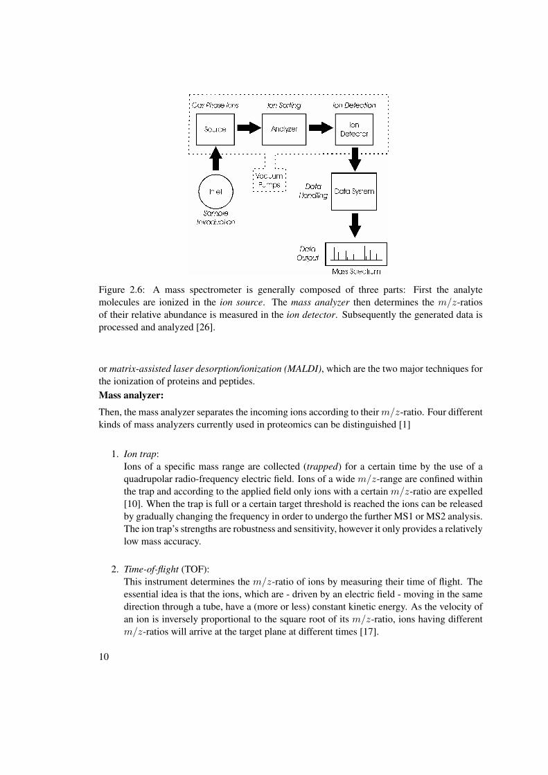
Figure 2.6: A mass spectrometer is generally composed of three parts: First the analytemolecules are ionized in the ion source. The mass analyzer then determines the m/z-ratiosof their relative abundance is measured in the ion detector. Subsequently the generated data isprocessed and analyzed [26].
or matrix-assisted laser desorption/ionization (MALDI), which are the two major techniques forthe ionization of proteins and peptides.Mass analyzer:
Then, the mass analyzer separates the incoming ions according to theirm/z-ratio. Four differentkinds of mass analyzers currently used in proteomics can be distinguished [1]
1. Ion trap:Ions of a specific mass range are collected (trapped) for a certain time by the use of aquadrupolar radio-frequency electric field. Ions of a wide m/z-range are confined withinthe trap and according to the applied field only ions with a certain m/z-ratio are expelled[10]. When the trap is full or a certain target threshold is reached the ions can be releasedby gradually changing the frequency in order to undergo the further MS1 or MS2 analysis.The ion trap’s strengths are robustness and sensitivity, however it only provides a relativelylow mass accuracy.
2. Time-of-flight (TOF):This instrument determines the m/z-ratio of ions by measuring their time of flight. Theessential idea is that the ions, which are - driven by an electric field - moving in the samedirection through a tube, have a (more or less) constant kinetic energy. As the velocity ofan ion is inversely proportional to the square root of its m/z-ratio, ions having differentm/z-ratios will arrive at the target plane at different times [17].
10

Figure 2.7: Scheme of a QExactive Orbitrap instrument [Thermo Fisher Scientific]
3. Quadrupole:A quadrupole consists of 4 circular - ideally, hyperbolic - metal rods which are alignedin parallel to each other. Between these rods a quadrupolar alternative electric field issuperposed on a constant field. The key idea is that according to the applied voltage onlyions with a certain m/z-ratio will pass through the quadrupole and reach the detector.Ions having a different ratio have unstable trajectories and will eventually hit one of therods [10].
4. Fourier transform ion cyclotron (FT-MS):This type of mass analyzer basically also traps desired ions. However, it does so by ap-plying strong magnetic fields. It provides a high sensitivity, mass accuracy, resolution anddynamic range. Despite these many advantages it is not widely used in proteomics re-search because of its high expense, operational complexity and especially its low peptide-fragmentation efficiency.
The mass analyzer can be seen as the key element of the mass spectrometer, since its task is theactual selection and filtering of ions, which is necessary to dsicrimante between them.Ion detector:Finally, the separated ions arrive in the ion detector where the relative abundance of ions foreach m/z-value (within the bounds of the resolution) is registered.As for the mass analyzer, there are several different ion detectors that are commonly used:
11

1. Faraday Cup:The Faraday Cup employs a very simple principle. The incoming ions hit its metal surfacewhich leads to the emission of electrons (so-called secondary emission) that induce acurrent. This current is then amplified and recorded.
2. Electron Multiplier:The electron multiplier extends the principle of a Faraday Cup. It consists of a vacuumtube containing a series of metal plates which are maintained at increasing electrical po-tentials. Incoming ions hit the first plate leading to the emission of electrons. These areattracted by the second plate which in turn emits electrons upon being hit. This way, acascade of secondary emissions is triggered at whose end typical amplification rates in theorder of 1:16 are achieved.
3. Orbitrap:The orbitrap consists of two electrodes, an inner spindle-like one and an outer electrodewhich envelops the inner one. Ions are injected tangentially into the orbitrap and trappedinside by the balance between the electrostatic attraction to the inner electrode and thecentrifugal force. The ions therefore cycle around the inner electrode forming rings whichoscilate along the electrode. This oscilation process is inversely proportional to the squareroot of the mass-to-charge ratio and can therefore be used to detect abundant ions.
2.2.2 The Shotgun-Proteomics approach
The term Shotgun Proteomics refers to a common form of non-targeted bottom-up proteomicsto analyze complex protein mixtures [42]. It is non-targeted because it does not aim to detect aspecific protein but rather tries to identify as many proteins as possible by comparison againstpossible theoretical matches in a database. The term bottom-up accounts for the prior digestionof the proteins into smaller peptides before running the MS/MS analysis.A shotgun proteomics workflow (see Figure 2.8) consists of the following steps:
• Digestion (Cleaving) of the proteins into smaller peptides by an enzyme (e.g trypsin).
• Separation of the peptides by liquid chromatography or high-performance liquid chro-matography (HPLC).
• Ionization of the peptides by electrospray ionization (ESI) or matrix-assisted laser des-orption/ionization (MALDI).
• Analysis of the peptide ions by tandem mass-spectrometry (MS/MS).
• Comparison of the generated data against databases in order to identify the proteins presentin the sample.
In the following these steps are described in detail.
12

Figure 2.8: Typical workflow of a shotgun proteomics experiment: First, the proteins are ex-tracted from the biological sample. Depending on the sample the resulting protein mixture canbecome very compley in terms of different proteins which are abundant in the mixture. The pro-teins are then cleaved into smaller peptides by proteolytic digestion leading to a more complexpeptide mixture. To reduce the complexity the peptides are seaparated by (multi-dimensional)LC and ionized using ionization techniques such as ESI or MALDI. These ions are then sub-jected to an MS/MS analysis. Finally, the analysis results are processed in order to determinethe abundant proteins [42].
2.2.2.1 Proteolytic digestion of large proteins into peptides
Proteolytic digestion is an important step to facilitate the analysis of the proteins cleaving theminto smaller peptides. This approach has several advantages: On the one hand, the ionizationof whole proteins leads to a great variety of charge states, whereas peptides are mostly two-fold or three-fold charged. Additionally, whole protein ions lead to huge isotope clusters in theresulting spectra, which further complicates their analysis, whereas peptides are usually smallenough, such that they usually only yield clusters containing around one to four isotopes. Thereason is simply that the smaller a molecule is, the less atoms exist in it that could possibly
13

be occurring not as the usual, most likely isotope variant but as a heavier one. Finally, theidentification of several peptides that can originate from the cleaving of a specific protein is amuch stronger proof for the correctness of the protein-identification than simply finding a matchfor the whole protein.
Thus, the initial step of the workflow is the proteolytic digestion, i.e. the cleaving of aprotein into smaller peptides by using a suitable endoproteolytic enzyme. These enzymes breakpeptide bonds at specific positions in the peptide, i.e. before or after certain nonterminal aminoacids. Unfortunately, this proteolytic digest is not always complete and it is possible that someof the specific cleavage sites are missed (so-called missed cleavages). Trypsin has proved tobe a suitable choice for this purpose, as it has been showed that Trypsin cleaves exclusivelyC-terminal to Arginine and Lysine residues. [32]. Having the highly basic amino acids Lysinand Arginine at the C-termini of the peptides also facilitates the ionization of these peptides,since they have a high affinity to protons. Another advantage is that a tryptic digest leads topeptides whose masses are in the preferred range for effective fragmentation by a subsequentMS/MS analysis, which is due to the fact that Arginine and Lysine each account for around 5%of the amino acids in a protein. Since there are 20 proteinogenic amino acids the protein is intheory cleaved after every 10-th amino acid, i.e. the average length of the resulting peptide is ca.10 amino acids. These factors have made Trypsin the most common choice when conducting ashotgun proteomics experiment.
2.2.2.2 Peptide separation by High-Performance Liquid Chromatography
The number of distinct proteins in a complex sample is too high to allow for identification usingonly a handful of scans. Moreover, the complexity of the sample is further increased by thedigestion of the protein mixture. Therefore, the peptides obtained after the digestion step mustbe separated, such that ideally only one peptide at a time is analyzed by the mass spectrometer.In general, there are several key characteristics according to which the peptides in the mixturecan be separated: solubility, size, charge and hydrophobicity. The technique of choice generallyused in shotgun proteomics is the reversed-phase high-performance liquid chromatography [1],which makes use of the hydrophobicity. In general, liquid chromatography employs two phases,a solid stationary one (also called the column) and a liquid one. The column contains certainchemical groups to which the peptides have a greater or lesser affinity, which causes them topass the column more or less quickly. In reverse-phase liquid-chromatography the solid phasecontains hydrophobic molecules whereas the liquid phase is highly hydrophilic. Consequently,the more hydrophilic a peptide is, the quicker it will pass through the column. In contrast,hydrophobic peptides will get caught more often on their way by intermolecular interactionswith the stationary phase, slowing down their progress. In order to accelerate the elution ofhighly hydrophobic peptides, which would bind to the column for far too long, concentrationgradients of organic compounds are used, i.e. the hydrophobicity of the liquid phase is graduallyincreased. The use of a gradient is opposed to the so-called isocratic elution methods, wherethe concentration of organic compounds remains constant through the whole elution process.Typically, the liquid phase contains 0.1 % formic acid and a gradient of 5 to 75 % acetonitrile isused. The time a peptide takes through the column from the moment it enters to the moment itelutes is referred to as its retention time.
14

The high-performance component of the name originates from the much higher pressures thatneeds to be applied to the column in order to maintain a constant flow-rate. This is necessary asthe column is made of much finer material than normal chromatography columns. This resultsin higher resolutions through better separation.
To further enhance the separation of peptides one can also employ two-dimensional or eventhree-dimensional liquid chromatography, where the separation is based on two or three criteria,respectively.
2.2.3 Peptide ionization in the ion source
Figure 2.9: Electrospray Ionization Process: The droplets eluating from the needle tip are sub-jected to an electrostatic field of around 2 kV. This causes the droplets to continuously explodeinto smaller droplets until they only consist anymore of the separate ions that were resolved inthem [29].
The two most commonly used techniques used for the ionization of peptides are ESI [16]and MALDI [20]. While MALDI can only be operated offline and is therefore usually used toanalyze simple peptide mixtures, ESI is more suited for a shotgun proteomics setup. The reasonis that ESI can couple liquid chromatography to mass spectrometry allowing an automated high-throughput analysis.In ESI a metal needle tip is added at the end of the LC-column, such that the eluate exitingthe column passes through it. A voltage of typically 2 kV is applied between the needle andthe opposing entrance of the mass spectrometer. The resulting electric field causes the eluate todisperse into a fine spray of charged droplets. With reducing droplet size a point is eventuallyreached at which the cohesive forces of surface tension are smaller than the repulsive forcesbetween the charges: A so-called Coulombic explosion occurs leading to a high number ofeven smaller droplets [2]. Finally, after repeated iterations of this process, ions of the analytesdissolved in these droplets are produced. The process is illustrated in Figure 2.9.
15

2.2.4 Tandem Mass Spectrometry
Even after undergoing proteolytic digestion and passing the liquid chromatography column thecomplexity of most peptide mixtures is still too high to already be sufficiently separated. For thisreason an effect called coelution occurs, where different peptides elute at the same retention time,which thus enter the mass spectrometer simultaneously. These peptides need to be separated inorder to be identified.To overcome these difficulties tandem mass spectrometry is used, which employs the workflowshown in Figure 2.10. This workflow consists of repeating cycles which in turn consist of the
Figure 2.10: The MS/MS-scan cycle: At the beginning of each cycle the most intense precursorions of a preceding MS1-scan are selected and subsequently isolated one after another for frag-mentation (Loop). This gives rise to the MS2-scans of the respective precursor ions showing theresulting fragment ions [44].
following steps:
1. MS1-scan:The instrument records an MS1-spectrum, i.e. for a defined m/z-range all currently elut-ing ions (also referred to as the Total Ion Current or simply TIC) are collected and an-alyzed. This spectrum shows the measured m/z-values together with the correspondingintensities. The intensity indicates the abundance of ions having the corresponding m/z-value. The higher the resolution chosen in the instrument settings the more well-definedare the resulting peaks (i.e. the smaller their width).
2. MS2-scan loop - fragmentation of selected precursors:This spectrum is then analyzed and the n most abundant peptides are selected for a subse-quent fragmentation analysis. This is also referred to as a Top-n method. In order to do so,one by one each of the selected peptides, which are also referred to as precursors, is nowisolated from the bulk of ions. I.e. a narrow m/z-window of usually 1 to 3 Da with theprecursor’s m/z-value at its center is applied to the TIC, isolating only ions whose m/z-value lies within this window. After collecting these specific ions for a preset amountof time or until a predefined ion threshold is reached they are sent into the collision cellwhere they are fragmented. For fragmentation to take place the ions are first activated inthe collision cell by elevating their energy levels to an excited state. The natural reduc-tion of the raised energy levels promotes fragmentation of the ions into certain fragmentions (this is explained more detailed later in this section). Finally, the m/z-ratios of these
16
resulting fragment ions are measured yielding an MS2-scan which shows the abundancesfor these fragments.
After all n precursor ions have been fragmented and analyzed the cycle repeats with the record-ing of a new MS1-scan.
Note that the mass analyzer usually also determines the charge state of the precursor ions.This can be done by quickly analyzing isotope patterns found in the spectra. When the chargestate z and the m/z-ratio of the ion are known, its molecular mass M can easily be calculatedby the following formula:
M = (m/z −H+) · z (2.2)
where z its charge state and H+ the mass of a proton, which is ca. 1.007276 Da.There are many settings that can be applied to control this general scheme. Besides the above-mentioned possibility of choosing the size of the isolation window, other important parametersinclude the dynamic exclusion list settings. Whenever an ion is chosen for fragmentation itsm/z-value is stored on the list for a certain amount of time. None of the m/z-values that arecurrently listed may be chosen for fragmentation. This way the multiple fragmentation andanalysis of peptides that dominate the TIC is avoided, such that there is more time to isolateother less intense peptides. Similarly, one can optionally define an inclusion list on which them/z-ranges are listed that contain peptides of special interest. Only ions whose m/z-value fallsinto the defined ranges are chosen for fragmentation. This is a useful setting when looking forspecific peptides that are part of a complex sample where it is likely that they might be too littleintense in comparison to the other ones.
2.2.4.1 Fragmentation of peptide ions by activation leading to MS/MS-spectra
An important step necessary to make tandem mass spectrometry possible is the fragmentationof the peptide ions. Modern mass spectrometers offer different activation types that can beapplied to achieve this fragmentation. The different activation types give rise to different kindsof fragment ions, since there are different possibilities to cleave peptides. Depending on theexact cleavage site the following pairs of fragment ions are distinguished:
• a- and x-ions.
• b- and y-ions.
• c- and z-ions.
The a-, b- and c-ions contain the N-terminus, and the x-, y- and z-ions the C-terminus. Thefragments are numbered according to the number of amino acids they contain additionally to theN- or C-terminus.Figure 2.11 shows the possible cleavage sites and gives an illustration of the established nomen-clature of the resulting fragment ions [37]. In the following the three most commonly-usedactivation types are introduced.
17

Figure 2.11: Possible Cleavage sites in a peptide and names of the respective fragments [45].
Collision-induced dissociation (CID) CID, sometimes also referred to as collision-activateddissociation (CAD), is the first technique used for the fragmentation of peptides. The precursorion is kinetically excited which is achieved through collisions with non-reactive gas molecules,such as argon or helium [43]. During each collision the imparted translational energy is con-verted to vibrational energy that spreads quickly within the molecule via all covalent bonds. Assoon as the activation energy required for a certain bond to be cleaved is reached the respectivefragment ions are formed. The amide bond chaining the amino acids together is the bond thatwill most likely break in a peptide ion [50], leading to the above-mentioned b- and y-fragments.Although this technique is very efficient, there are some major drawbacks to be considered:Fragment ions having an m/z-ratio of less than around one third of the precursor ion m/z arenot trapped properly due to physical limitations. This effect is commonly referred to as the low-mass cut off. Furthermore, the recorded MS2-spectra suffer from relatively low mass accuracyand resolution [31]. The former issue is particularly problematic when applying quantitativeproteomics, since the crucial information about the ratios between reporter ions, which havemasses lower than 132 Da, is lost.To overcome the low-mass cut off problem Thermo Fisher Scientific has developed the Pulsed QCollision Induced Dissociation technique (PQD), which is exclusively available in their instru-ments. This approach promises to yield mass spectra qualitatively comparable to CID spectrawithout losing the information in the lower m/z regions and thus making them usable for quan-titative proteomics.
Higher-energy collisional dissociation (HCD) A more substantial improvement has beenachieved with the development of HCD. While on the one hand making the full mass-rangeof the MS2-spectrum available, this technique additionally provides high mass accuracy andresolution [31]. In principal, it is a higher-energy variant of CID. Precursor ions are also ki-netically excited by collision with gas molecules (typically N2) in order to break up into thecharacteristic fragment ions.The resulting spectra have a similar pattern as the ones obtained by CID, i.e. the fragmentation
18

products that can be measured are the b- and y-fragments. Additionally, however, the fragmentsfrom the low mass region, such as the y1-, y2-, b1- and b2-fragments are also detected and appearin the spectra.
Electron transfer dissociation (ETD) This method is based on the previously developedmethod of Electron capture dissociation (ECD) [52]. Like its predecessor ETD has been devel-oped for the use with ion traps, where multiply protonated peptides are confined and subjectedto low-energy electrons. The uptake of the electrons is an exothermic reaction and leads to aspecific cleavage of the peptides into c- and z-type fragment ions in contrast to the two above-mentioned activation types. However, maintaining the dense accumulation of electrons aroundthe precursor peptide necessary to induce the electron uptake remains technically challengingfor some instruments. Therefore, in ETD, contrary to ECD, negative ions (e.g. anthracene) areused in order to achieve the electron uptake of the peptide. Instead of simply capturing a freeelectron a transfer of an electron from the anion to the peptide takes place, promoted by the factthat anions with very low electron affinities are used [43].A big advantage of this method over CID or HCD is that the precursor retains labile PTMs asthe fragmentation is not achieved by an increase of the internal energy. The downside is thelimited applicability to doubly charged precursor ions, which can, however, be overcome by theapplication of a supplemental activation method to those precursors that are still intact after ETDfragmentation [41].
2.2.5 Analysis of generated mass spectrometry data
2.2.5.1 Spectrum Preprocessing
A typical shotgun-proteomics experiment can generate between 40000 and 50000 MS2-spectrain an average 3h run. This amounts to roughly 3 GB of data. To cope with the vast amountsof data being produced preprocessing steps, such as spectrum-filtering and -manipulation arenecessary. All the more since on average only around 50% of the MS2-spectra can be confidentlyidentified.At this point of the workflow the methods studied and developed in this thesis are settled. Theywill be explained in chapters 3 and 4.
2.2.5.2 Database Search
In order to automatically identify peptides and proteins, many different database search engineshave been developed [7,9,15,35]. The general principle of the search is common to all of them:The protein database is digested in silico, i.e. the smaller peptides into which the protein cantheoretically be cleaved by a complete cleavage are generated. The experimental MS2-spectraobtained from the mass spectrometer are now compared against the fragment spectra of thesetheoretical peptides. Depending on the search settings a certain number of possible theoreticalpeptides are to be considered for the explanation of a given MS2-spectrum. All possible matchesare then evaluated using statistical approaches yielding a scoring depending on how probable thematches are. The matching peptides are then ranked according to the score they obtained. This
19

process is illustrated in Figure 2.12. Notably, this final step of the proteomics workflow is most
Figure 2.12: Basic workflow of database search engines: The proteins from a selected databaseare digested in silico into smaller peptides. This yields a list of these peptides and their corre-sponding molecular masses. For an MS2-spectrum there are a number of candidates whose massis close enough to the precursor mass, s.t. they are considered as an explanation of the MS2-spectrum. The MS2-spectrum in question is now matched against the theoretical MS2-spectraof the candidate peptides and each match is scored according to how good it is [44].
likely the most versatile one. As it is the crucial step towards making sense of the measureddata it is also highly customizable. The first and most important settings are the choice ofthe database that should be used (human, yeast, etc.), the enzyme that has been used for theproteolytic digestion, the fragment ion types to match and the choice of possible dynamic andstatic amino acid modifications. These modifications can either be due to chemical derivatisationduring sample preparation or post-translational modifications, both leading to a shift in peptidemass. Therefore, they additionally need to be taken into consideration when searching for amatching peptide. Clearly, adding modifications exponentially increases the search space.Following these basic settings there are - depending on the specific search algorithm - severalfurther parameters that have to be specified. As there are so many different settings and moreovermany different settings for different search engines, we only briefly mention the most generalones that are common to most search engines. Most importantly tolerance windows for peptidemasses and fragment ion masses can be set. The former narrows the possible candidate peptidesto be considered when looking for a match to a certain given mass while the latter narrows thetolerance within which the fragment ions may deviate from the theoretical fragments of a peptidebeing matched. The tolerance of the search algorithm is usually even further adaptable by settingthe maximum amount of missed cleavage sites accommodating for the fact that the proteolyticdigestion does not work perfectly.
20

2.2.5.3 Evaluation of search results
The output of a database search is a list of so-called peptide spectrum matches (PSMs) mappingthe submitted spectra to peptides. In general, however, we do not have any information aboutthe quality of these results. Elias and Gygy pointed out three reasons why it is necessary to havea means for describing the quality of the search result [14]:
1. The database used for the search may be incomplete i.e. some of the target peptides maynot be part of the search space and can never be found.
2. Some spectra may be recorded because of chemical background noise and will thereforelead to false interpretations as random entries in the database might match well enough.
3. In some cases an incorrect peptide matching to a spectrum may be assigned a higher scorethan the correct interpretation.
It is therefore necessary to establish criteria determining the level of confidence with whichthe results can be trusted. Moreover, it must be possible to automatically filter search resultsaccording to these criteria, such that PSMs that are most probably incorrect can be filtered out.An automatic validation is especially crucial in shotgun proteomics experiments where a vastamount of data is generated and the search results can no longer be validated manually.A natural quality criterion of database search results is the false discovery rate (FDR). In general,the FDR is given by
FDR =FD
FD + TD(2.3)
where in FD is the number of false discoveries and TD is the number of true discoveries.In our case the former corresponds to the spectra that have been assigned an incorrect peptide,the latter to the spectra that have been identified correctly. Clearly, FD + TD is equal to thetotal number of PSMs. However, under normal circumstances it is impossible to determine theFDR of a search result as it is - of course - unknown which of the PSMs are the true and whichthe false positives, respectively.
To overcome this problem a method of estimating the number of false discoveries in a resultlist has been proposed: The target-decoy search strategy [13, 25]. In this approach two differentdatabases are used for the search. On the one hand there is the original database against whichthe search is conducted as usual (the target database). On the other hand an additional databasecontaining only non-existing peptides is employed (the decoy database). Consequently, everyPSM mapping a spectrum to a peptide defined in the decoy database is a false positive by defi-nition.For the estimation of the number decoy hits it is necessary to determine the ratio of decoy to tar-get hits (rd/rt) in the search space. This ratio leads to the multiplicative factor f that reflects thedecoy bias of the chosen approach, such that, after observing a certain amount of decoy hits (d)and knowing the frequency ratio between target and decoy hits in the database one can calculatethe number of false positives [14].
f =1
rd(2.4)
FP = d · f (2.5)
21
Ideally, the ratio of decoy to target hits is 1:1, such that a random hit may just as likely be adecoy hit as a target hit. I.e. rd = rt = 0.5 and thus f = 2.
In order to achieve this ideal ratio the following criteria must be met by the decoy databasewith respect to the target database:
1. The amino acid distributions among the peptides should be similar.
2. The protein length distribution should be similar.
3. The total number of proteins should be similar.
4. The number of the theoretical peptides predicted for the digest of the proteins should besimilar.
5. The databases may have no predicted peptide in common.
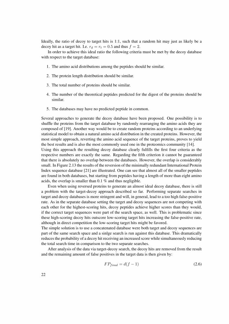
Several approaches to generate the decoy database have been proposed. One possibility is toshuffle the proteins from the target database by randomly rearranging the amino acids they arecomposed of [19]. Another way would be to create random proteins according to an underlyingstatistical model to obtain a natural amino acid distribution in the created proteins. However, themost simple approach, reverting the amino acid sequence of the target proteins, proves to yieldthe best results and is also the most commonly used one in the proteomics community [14].Using this approach the resulting decoy database clearly fulfills the first four criteria as therespective numbers are exactly the same. Regarding the fifth criterion it cannot be guaranteedthat there is absolutely no overlap between the databases. However, the overlap is considerablysmall. In Figure 2.13 the results of the reversion of the minimally redundant International ProteinIndex sequence database [21] are illustrated. One can see that almost all of the smaller peptidesare found in both databases, but starting from peptides having a length of more than eight aminoacids, the overlap is smaller than 0.1 % and thus negligible.
Even when using reversed proteins to generate an almost ideal decoy database, there is stilla problem with the target-decoy approach described so far. Performing separate searches intarget and decoy databases is more stringent and will, in general, lead to a too high false-positiverate. As in the separate database setting the target and decoy sequences are not competing witheach other for the highest-scoring hits, decoy peptides achieve higher scores than they would,if the correct target sequences were part of the search space, as well. This is problematic sincethese high-scoring decoy hits outscore low-scoring target hits increasing the false-positive rate,although in direct competition the low-scoring target hits might be favored.The simple solution is to use a concatenated database were both target and decoy sequences arepart of the same search space and a sinlge search is run against this database. This dramaticallyreduces the probability of a decoy hit receiving an increased score while simultaneously reducingthe total search time in comparison to the two separate searches.
After analysis of the data via target-decoy search, the decoy hits are removed from the resultand the remaining amount of false positives in the target data is then given by:
FPfinal = d(f − 1) (2.6)
22
Figure 2.13: Peptide overlap between the human protein sequences within the minimally redun-dant International Protein Index sequence database (target) and the reversed sequences createdout of them (decoy) [13].
Figure 2.14 shows an overview on the target-decoy search workflow (a) and illustrates the dis-tribution of target and decoy hits among all peptide hits for the different ranks assigned bySEQUEST (b-d). The analysis shows that within the first-rank hits the number of reported targetsequences is much higher than the number of decoy sequences. In the lower ranks neither se-quence set is favored. This confirms the correctness of the approach as the first rank is the mostprobable hit (the one that is most likely to be correct) while the lower ranks are assigned to lessprobable sequences and are thus more likely random hits. As intended for random hits, the ratioof target to decoy sequences is 1:1. The aforementioned considerations suggest a fairly simpleprocedure to obtain a result list filtered to abide a desired FDR. Algorithm 2.1 describes a naiveand rough method to set a certain FDR for the results list. The first line is a direct consequenceof the fact that for peptides containing less than 8 amino acids there is a considerable overlap intarget and decoy sequences. Hence, they violate the precondition that the two databases musthave no predicted peptides in common and must therefore be filtered out from the PSM list be-fore setting the FDR. Another problem are hits the search engine has ranked lower than 1. Asshowed above, for the lower ranks the ratio of target to decoy hits is 1:1 and thus the results are
23

Figure 2.14: a) The target-decoy search workflow. b) Example of PSMs returned by a SEQUESTsearch. The percentages of matching spectra from both target and decoy database are shown forthe top-10 ranking peptide hits. c) The same search but with previously falsified MS/MS spectra.d) The same search but with previously altered precursor masses [4].
mere random hits. Therefore, in order to correctly set the FDR, the lower-ranking results haveto be filtered out, as well, which is done in line 2 of the procedure. Afterwards, a score thresholdis continuously adapted, until the ratio of target to decoy hits corresponds to the desired FDR.After removal of the decoy hits, the percentage of incorrect hits in the resulting PSM list abidesto the set FDR.
Note that it is of course also possible to set other confidence criteria than the search enginescore to define the FDR. The following list provides examples of further quality criteria that canbe used for defining the confidence of PSMs:
• The ∆Score, i.e. the score difference between the rank 1 and the rank 2 peptides.
• The accuracy of the precursor mass.
• Number of missed cleavage sites.
• How often does the matched peptide match other MS2 spectra.
Moreover, combinations of several criteria are possible. This concept is, for instance, used in thePercolator algorithm [18], which applies a machine learning algorithm to determine the relevantfeatures of the spectra in order to come up with a suitable set of criteria and correspondingweighting factors.
24

Algorithm 2.1: Set False Discovery RateInput : PSMs (list of search results),
FDR (desired false discovery rate)Output: PSMs, filtered to FDR
1 Remove all hits for peptides smaller than length 8 from PSMs;2 Remove all hits for peptides with search engine rank smaller than 1 from PSMs;
3 FDRcur ← 1 ;4 Score← 0 ;5 while FDRcur >FDR do6 Score← Score + Increment ;7 Remove all hits for peptides with a score smaller than Score from PSMs;8 t← number of target hits ;9 d← number of decoy hits ;
10 FDRcur = dt ;
11 end12 Remove all decoy hits from PSMs;13 return PSMs
Note that regarding identified peptides the FDR is in general larger than the threshold set atthe PSM level. This is due to the fact that several correctly identified spectra may be explainedby the same peptide. On the other hand, incorrect PSMs distribute randomly over the peptidesin the database, as they represent hits by mere coincidence.
2.3 Definition of relevant data structures
In the following a short overview on the data that is output by a mass spectrometer is provided.We list the information that is stored in an output file, and which can generally be seen asgiven from the viewpoint of the designed algorithms. Unless stated otherwise, the preprocessingalgorithms are applied to one MS2-spectrum at a time and thus their input usually consists onlyof one such spectrum. However, should it be necessary, the rest of the data may be accessed,too, by reading directly from the raw data file.
2.3.1 The .RAW file format
The standard file format of the output files produced by Thermo Fisher Scientific mass spectrom-eter instruments is the Thermo Xcalibur file format (.RAW). Since this is a proprietary binaryformat it can only be read by either the Thermo Scientific Xcalibur software or via Thermo’sMSFileReader libraries. Parts of the developed programs therefore use the functionality pro-vided by the XRawfile2.dll, version 2.1.1.0.
Most importantly a .RAW file contains all spectra (MS1 and MS2) recorded by the massspectrometer which can be accessed by their unique running number. The spectra are enu-
25

merated in the order in which they have been recorded, i.e the first spectrum is the first MS1-spectrum, followed by the associated MS2-spectra, if there are any. Then, the next MS1-spectrum follows, and so on.
Additionally, for each spectrum a collection of additional information, such as retentiontime, total ion current etc. and certain instrument specific control data and correction factorsare stored. Although this information is per se not necessary for the follow-up identification orquantification of peptides, it is still valuable for further analysis to detect flaws in the workflowand devise ways of improving it.
Finally, reports about the defined methods and settings are available for each spectrum.Note that the crucial information, i.e. the spectrum data itself, is of course also stored in other
file formats. The algorithms that are described in this thesis can therefore also be implementedto be operated with these other file formats.The most popular open data format that should be mentioned is mzML.
2.3.2 Formal definition of mass spectra
For computational means, a spectrum can formally be defined as a list of peaks, where a peak(and the ion indicated by it) is defined by a structure consisting of the following attributes:
Mass Peak dataName Data Type Abbreviation DescriptionPosition double m/z The mass per charge ratio m/z of the ion, in a mass
spectrum this is where the centroid of the corre-sponding peak is.
Intensity double I The intensity of the ion current measured in ions/sCharge State int z The charge state of the ion. Note that this informa-
tion is not necessarily required and the mass spec-trometer is not able to determine the charge state forevery peak that is recorded!
The column Abbreviation denotes the name of the attribute as it will be used in algorithm de-scriptions within this thesis. E.g. the intensity of a peak p will be referred to as p.I .
Instead of having a list of peaks centroids, an alternative, and more precise representationof a mass spectrum can be given by listing not the peak centroid data but the profile points eachpeak consists of. The profile representation requires roughly ten-fold as much memory.
In both cases the peaks (or the profile points) in the list are sorted ascendingly by their m/zvalues. The following figure shows an excerpt of an actual MS1-spectrum recorded with anLTQ Orbitrap XL instrument. It lists the position and the intensity of one specific peak’s profilepoints.
For MS2-spectra additional information is stored, since an ion from the MS1-spectrum hasto be selected to give rise to an MS2-spectrum illustrating the fragments of the respective ion,commonly referred to as the precursor. The following attributes constitute the most commonlyused precursor data associated with an MS2-spectrum:
26

. . .436.79187 391178.8436.79360 4404735.0436.79532 11392973.0436.79704 17311702.0436.79877 17713638.0436.80049 12358349.0436.80222 5574961.0436.80394 2130796.0436.80567 1400039.8. . .
Figure 2.15: Excerpt of an MS1-spectrum schowing the m/z-values and intensities of someprofile points.
MS2 Precursor dataName Data Type Abbreviation DescriptionPrecursor Position double prec.m/z The mass per charge ratio m/z of the
precursor ion.Precursor Intensity double prec.I The intensity of the precursor ion.Precursor Charge State int prec.z The charge state of the precursor ion.Precursor Scan Number int prec.scan The number of the spectrum the precur-
sor was selected from.Precursor Isolation Width double prec.isolation The width of the window applied
around the precursor m/z determiningwhich m/z-range has been collectedfor fragmentation.
Activation Type string prec.activation Which activation type was used for pre-cursor fragmentation.
27

Last but not least, there is a collection of header data attached to each spectrum containingfurther valuable information. The following table provides an overview on the most importantparameters that are available in the header.
Spectrum header dataName Data Type Abbreviation DescriptionScan Number int header.scan The running number used to identify
the spectrum.Retention time double header.rt The point in time at which the spectrum
was recordedIon Injection Time double header.ionInject The amount of time (usually in ms) the
ions have been collected before theywere measured.
Low Mass double header.lowMass The lower end of the mass range thatwas considered for the scan.
High Mass double header.highMass The upper end of the mass range thatwas considered for the scan.
28

CHAPTER 3MS2 - Spectrum Manipulation
3.1 Motivation
One way to deal with the vast amount of data generated by a shotgun proteomics experimentis the manipulation of MS2-spectra in a preprocessing step preceding the database search. Thealgorithms described in this section directly target the peak list in a spectrum with the goal of re-moving unnecessary peaks to facilitate the follow-up analysis done by the search engine. Sincethe number of possibilities that have to be considered as possible fragment ions is reduced thescore of correct identifications is increased. Furthermore, the probability of incorrect identifica-tions is reduced as there are less possibilities for random hits. Of course, these two argumentsonly hold true, given the assumption that the algorithm works correctly and removes the super-fluous peaks it is actually targeting. An additional advantageous side-effect by the reduction ofpossibilities is the reduction in runtime of the search.
In the following the developed methods for deisotoping and charge-deconvolution of spectra,as well as the ideas they are based on are described. Furthermore, ideas on further possibilitiesto improve spectrum quality are outlined.
3.2 Deisotoping
As described in section 1.1, a peak in a spectrum (MS1, as well as MS2) indicating the abun-dance of an ion is usually accompanied by a certain number of shifted peaks. The reason for thiseffect is the fact that for many chemical elements there are isotope variants that occur naturally.Isotopes are atoms whose atomic nuclei contain the same number of protons but a different num-ber of neutrons, therefore having a different atomic mass.Table 3.1 lists the naturally occurring isotopes for the elements occurring in the proteinogenic1
amino acids, the first variant of each element is the most abundant (and lightest) one. Note thatthe mass difference between e.g. a 1 13C and a 2 13C isotope is not exactly the mass of the
1Proteinogenic amino acids are those amino acids occurring in proteins
29

Element Atomic mass (Da) Natural abundance (%)Carbon12C 12.0000000 98.9013C 13.003354838 1.10Hydrogen1H 1.007825032 99.9852H 2.014101778 0.015Nitrogen14N 14.003074005 99.63415N 15.000108898 0.366Oxygen16O 15.994914622 99.76217O 16.999131501 0.03818O 17.999160419 0.200Sulfur32S 31.972070690 95.0233S 32.971458497 0.7534S 33.967866831 4.2136S 35.967080880 0.02
Table 3.1: Naturally occurring isotopes of the elements in proteogenic amino acids. The atomicmasses are according to [3], the isotopic abundances are taken from [6]
additional neutron2 the 2 13C has in comparison to the 1 13C, but somewhat less. This is due toa phenomenon called mass defect, which - simply put - states that the mass of the bound system,i.e. the whole nucleus, is less than the sum of the masses of the unbound system, i.e. the separateprotons and neutrons.
Consecutively, two molecules of one and the same compound may have a different totalmass as they could contain different isotopes.We call the variant consisting of the most abundant isotope variatns, i.e containing only lightatoms, the monoisotopic variant and thus the corresponding peak in the spectra is referred to asthe monoisotopic peak. As it is the lightest variant of the compound this peak appears the farthestleft on the m/z-axis. If the same compound also occurred having one or more of these isotopesexchanged with their heavier variants, this would lead to additional peaks in the spectrum furtherto the right on the m/z-axis.Hydrogen and carbon are the most abundant atoms in an amino acid. But as the probabilityfor the occurrence of an 2H atom is only 0.015%, compounds containing them are so rare thatthey usually do not yield peaks that are intense enough to be distinguished from random noise.On the other hand, with 1.10%, the probability for carbon to occur as the heavier variant (13Cinstead of 12C) is high enough, s.t. it is likely that among all the C atoms of a certain molecule,there will be one 13C isotope. Likewise, for bigger compounds (containing more C atoms) there
2The mass of a neuron is ∼ 1.00866 Da
30

is also a considerable amount of molecules containing two, three or even more 13C isotopes.These heavier molecules also lead to well-visible peaks in the spectrum indicating them.Note that although for sulfur atoms the probability for a 34S isotope is comparably high, theeffect is barely visible in lower m/z-ranges. The reason is that there are only two amino acidscontaining sulfur, namely cysteine and methionine, which have a natural abundance of 1.9% and2.3%, respectively [39].
Therefore, as an indication for a certain ion we can usually observe a so called isotopepattern in the spectrum, which is composed of peaks indicating variants of the ion containing adifferent number of 13C isotopes. Since replacing a 12C by a 13C isotope will increase the totalmass of the ion by roughly 1 Da, we observe for a monoisotopic peak with an m/z value of vand the charge state c a shifted peak at v + n
c for the ions containing 1 13C isotopes, a peak atv + 2n
c for the ions containing 2 13C isotopes, etc. Here, the n stands for the mass differencebetween 12C and 13C which is ca. 1.003354838. Figure 3.1a shows an isolated example of atypical isotope pattern, consisting of the monoisotopic, as well as the 1 13C and the 2 13C peaks,as it could occur in a spectrum.
As common search engines do not take additional isotope peaks into account but only relyon the monoisotopic peak to identify fragment ions, it is a reasonable approach to see thesesuperfluous peaks as noise and remove them from the spectrum.
We therefore experimented with several ideas, starting from the approach by Savitski etal. [38], in order to develop a reliable way of determining isotope patterns in MS2-spectra andcleaning them thereof, s.t. only the monoisotopic peaks remain. Every peak, that is not accom-panied by an isotope pattern, should remain untouched. This general procedure is referred to asDeisotoping. Figures 3.1a and 3.1b show an isotope pattern before and after deisotoping.The following sections give a detailed description of the ideas that we experimented with alongwith a short summary of the results achieved with the respective method.
3.2.1 A simple Deisotoping algorithm
The deisotoping approach we started with has originally been implemented by its authors as partof their H-Score approach [38], which we do not further explain here, as it is out of the scopeof this thesis. As the aim of H-Score was the introduction of a new scoring scheme for highmass accuracy data, the deisotoping method incorporated in it is a suitable starting point for thedevelopment of new sophisticated deisotoping algorithms for the high mass accuracy spectra wewant to optimize.
The algorithm makes use of the above-mentioned distance of nc between consecutive iso-
topes for a c-fold charged analyte ion. It traverses the peak list backwards, i.e. starting fromthe peak with the highest m/z-value towards the peak with the lowest one. For each peak piit inspects, if there is a previous peak pj having the distance n
c for c ∈ [1..p] (with p being theprecursor charge). Of course, inaccuracies in the data have to be accounted for, which is whya certain tolerance value has to be applied, the authors used ±0.025 Da, here. Additionally, asimple plausibility criterion is checked: From the two peaks in question, the intensity of the firstpeak, i.e. the one with the greater m/z-value, may be at most twice as high as the intensity ofthe second one. If these two criteria are fulfilled, the second peak is marked for removal, whichis done by simply setting its intensity to 0. In the end, every peak with intensity 0 is removed
31

(a) Example of a typical isotope pattern. The monoisotopic peak of an ion at 239.01254Da (also referred to asthe 12C or the 0 13C peak) is followed by the 1 13C peak at 240.0159Da and the 2 13C peak at 241.01678Da
(b) The same situation after deisotoping. Only the monoisotopic peak remains in the spectrum.
Figure 3.1: Simple isotope pattern, before (a) and after (b) deisotoping
from the peak list.Algorithm 3.1 gives a pseudo-code of the described procedure.
This algorithm is simple and straightforward. Indeed, a preprocessing of the MS2-spectrausing this method improves the identification rate compared to the search of unprocessed spectra(for a detailed comparison see section 5.2). We could even see an improvement for CID spectrawhich have lower mass accuracy. Obviously, the algorithm leaves room for several improve-ments having some considerable drawbacks:
1. The tolerance window of ±0.025 Da is too generous considering the high resolution ofHCD spectra.
2. The algorithm marks detected peaks too quickly, i.e. whenever two peaks fit the criteria,the second peak is marked. This procedure can be problematic when overlapping patterns
32

Algorithm 3.1: Deisotoping as implemented by Savitski et al. [38]Input : A list of (m/z, I)-pairs, peaks, of length N ascendingly ordered by m/z
Structure containing precursor ion information, precA value defining the accuracy tolerance of the isotope search, tolerance
Output: Deisotoped peaks list
1 n← 1.0033548; // mass difference between 12C and 13C2 for i← N to 1 do3 for j ← i− 1 to 1 do4 for c← prec.z to 1 do5 if Abs(peaks[i].m/z − peaks[j].m/z - n) ≤ tolerance and
peaks[i].I > peaks[j].I/2 then6 peaks[j].I← 0 ; // mark this peak for removal7 end8 end9 end
10 end
11 foreach peak p in peaks do12 if p.I = 0 then13 Remove p from peaks14 end15 end
occur. A simple example is depicted in Figure 3.2.
Figure 3.2: Overlapping isotope patterns: Here, the three annotated peaks form an isotope pat-tern for charge state z = 1. The algorithm, however would also remove the two additional peaks,since they would fit in an isotope pattern with charge state z = 2.
33

3. The first peak falling in the tolerance window is marked as an isotope peak. However,there may be another peak having a distance closer to the expected one. Of course, thispeak would then be a better match and should be the only one that is marked. Instead,every peak that could be a possible isotope is marked.
4. Two consecutive peaks having the correct distance are, in general, seen as isotopes. Thechosen plausibility criterion, only rejecting such two peaks, if the second peak is at leasttwice as high as the first one, is a too simple way of modeling natural isotope abundances.Thus, almost every time when two peaks have the correct distance, they are recognized asindicating isotopes and consequently, the second peak is removed.
Generally spoken, these issues can be summarized by the observation that the algorithm is some-what inaccurate and too little restrictive. It simply removes too many peaks from a spectrum.
We therefore try to overcome these issues by modifying the original algorithm accordingly.
3.2.2 Improving the original algorithm
The first issue can be solved rather easily by simply reducing the size of the tolerance window.To this end we implemented a variable user-definable tolerance window allowing for more re-strictive tolerances. However, test runs with a tolerance of ±0.02 Da, ±0.015 Da, ±0.01 Da,±0.005 Da and ±0.001 Da did only show a slight but not significant improvement in the num-ber of PSMs. As can be seen in the experimental results in section 5.2, the optimal deisotopingtolerance seems to be around 0.015 Da, or 15 mmu, for HCD spectra.
In order to cope with the second problem, we slightly modify the existing algorithm. Insteadof marking peaks for removal, as soon as they are found, the possible isotope patterns for thecurrent peak under consideration of every charge state are stored in a list. Additionally, eachpattern is evaluated by a simple scheme, resulting in a score for this pattern. After performingthe search for all possible charge states, the pattern with the best score is then chosen and itspeaks (except for the monoisotopic peak, of course) are marked for removal.The score of a possible isotope pattern P consisting of n isotope peaks beside the monoisotopicone is given by the sum of the distance of each peak pi’s observed position pi.poso from itsexpected theoretical position pi.post.
score(P ) =n∑
i=1
|pi.poso − pi.post| (3.1)
This method assumes the best-scoring possible isotope pattern to be the actual one. It is thereforemore cautious than the original approach as it keeps peaks in the spectrum that are less likelypart of the sought isotope pattern.
In a similar way the third issue of the original algorithm could be handled. When lookingfor possible isotope peaks within the tolerance window, we do not accept the first match butrather look further for any other possible matches. Again, all possible peaks that would matchthis specific isotope peak are stored in a list. Finally, the best-fitting peak is chosen, i.e. the peakwhose deviation from the expected distance to the previous isotope peak is smallest.
However, this approach only reduced the number of PSMs and was therefore discarded.
34

3.2.2.1 Expected isotope-ratio determination by averagine modeling
The last issue is the most difficult one to deal with, since modeling the isotope abundance ratiosrequires an adaptive approach that is strongly dependent on the number of C-atoms containedin the respective molecule. Naturally, we do not have any information about the composition ofthe molecule prior to the search. However, its mass is known, which allows an estimation of theratios.In order to have an admissible estimation of the isotope ratios of a given molecule, the the-oretical isotope intensity ratios of a poly-averagine [39] (i.e. a peptide consisting of multi-ple averagines) of the same mass are used. Averagine is the average amino acid, a theoret-ical construction that has been developed based on the statistical occurrences of the aminoacids from the PIR protein database [49]. This model amino acid has the molecular formulaC4.9384H7.7583N1.3577O1.4773S0.0417 and an average mass of 111.1254 Da. As described above,the more C atoms there are in a peptide, the higher the probability that one, two, three or moreof these C atoms are actually 13C and not 12C isotopes.This is easy to see. We can formulate the question for the number of 13C isotopes in a moleculeas a serial experiment in which the C-atoms are independently examined one by one yieldingeither 13C or 12C as result. This is exactly what is modeled by the Binomial distribution. Thus,the probability for having k 13C-isotopes in a molecule containing n C-atoms in total is givenby
Pr(X = k) =
(n
k
)pk(1− p)n−k , where p = 0.011 (3.2)
Statistics suggests that these are also the average intensity ratios we can see when studying therespective isotope peaks. Figure 3.3 illustrates the probabilities for peptides consisting of anincreasing number of averagines to contain 0, 1, 2, or 3 13C isotopes. The Figure suggeststhat a more fine-grained acceptance criterion is needed. Certainly, the criterion chosen in theoriginal algorithm is fulfilled by any two isotopes of molecules up to 3333,762 Da (the mass ofa molecule consisting of 30 averagines). However, the problem lies in the opposite cases, whenthis criterion seems far too relaxed. Consider for example the 12C and the 1 13C isotopes of apeptide consisting of two averagines. The ratio between the intensities of the two peaks shouldbe around 1 to 10. Now, if we have a spectrum in which there are two peaks at roughly 220 Dahaving the distance expected from two isotope peaks but a ratio of 1 to 1, which considerablydiffers from the expected one, the original algorithm would still consider these peaks isotopesand delete the second of those from the spectrum.
These considerations suggest that an algorithm that uses a more sophisticated acceptancecriterion taking the actually expected ratios into account should be more accurate and thus yieldbetter results.We therefore analyzed 103431 MS2-spectra recorded by a Thermo QExactive instrument mea-suring a 1 µg HeLa sample to find out how well this theoretical model fits to actual data. Theanalysis was done in the following way:
1. For every isotope pattern found in the spectra select the monoisotope peak and calculateits uncharged mass m.
2. Calculate how many C-atoms there are in a poly-averagine of the same mass.
35

Figure 3.3: Probability distribution for the number of 13C-isotopes in a poly-averagine moleculedepending on the number of averagines in the molecule.
3. Calculate the theoretical intensities p0theo, p1theo, p2theo and p3theo for the 0 13C, 1 13C, 2 13Cand 3 13C isotopes, respectively using formula 3.2. Note that the calculated number n ofC-atoms is usually not an integer. Therefore we perform a linear interpolation betweenthe rounded down and rounded up values, i.e.:
P (X = n) = P (X = bnc)) · (n− bnc)) + P (X = dne)) · (1− (n− bnc))), (3.3)
where bnc and dne denote the applications of the floor and the ceiling functions to n,respectively.
4. Calculate the sum of the first 4 peaks in the pattern in order to determine their percentagesof this total intensity: p0obs, p1obs, p2obs and p3obs.
5. Compute the ratio ri =pitheopiobs
for 0 ≤ i ≤ 3.
Clearly, in an optimal fit every such calculated ratio is exactly 1. To obtain an extensive overviewthe data was plotted in the three dimensions, m/z and intensity (both taken from the monoiso-tope peak), as well as the ratio. Note that the ratio has been log2 - transformed for the plots,s.t. the range is compressed and optimally-fitting data points lie on the plane ratio = 0. Thefollowing plots show the data collected for each of the four isotopes separately, focusing on theintensity-ratio plane (left) and the m/z-ratio plane (right). The study of these plots leads to twoconclusions:
36

1. The ratio is clearly correlated to the intensity and is better, the higher the intensity is.
2. The ratio is not directly correlated to them/z-value of the peaks. Although the plots mightsuggest some kind of correlation, the different trends for the certain isotope peaks showthat this is indeed just a reflection of the correlation with the intensity. The explanation issimple. As Figure 3.3 also shows, for ions with lower masses, the intensity of the 1 13Cpeak - and moreover the 2 13C and 3 13C peaks - is relatively small in comparison tothe 12C. Especially if the isotope peaks are so small, that they are close or beneath thenoise level, it is therefore very likely that the percentage of the total intensity is heavilydistorted.Thus, a decent fit can only be seen for the 12C and the 1 13C isotopes. Regarding the othertwo, a general tendency can be seen but the variance is too high.
(a) (b)
Figure 3.4: 3d-plot showing the ratios of the measured against the theoretical intensities for the12C isotopes.
Consequently, we developed an algorithm that makes use of this correlation with the aim ofrejecting patterns for which the isotope ratios are not good enough. The principle is the same asfor the conducted spectra analysis. Additionally, after step 5 as described above, the computedratios ri are used for evaluation. However, as a conclusion of the analysis, we only considerratios r0 an r1, as only for those the correlation is good enough to be used as a quality criterion:We demand of both ratios to be greater than a given threshold value. If this is the case, theisotope pattern is accepted, and all but the monoisotope are removed.
Unfortunately, testing several ratio thresholds, as well as intensity thresholds did not signif-icantly improve the performance in comparison to the original approach. Moreover, it seems
37

(a) (b)
Figure 3.5: 3d-plot showing the ratios of the measured against the theoretical intensities for the1 13C isotopes.
(a) (b)
Figure 3.6: 3d-plot showing the ratios of the measured against the theoretical intensities for the2 13C isotopes.
sample-dependent, if the method yields any benefit at all or if it even reduces the number of
38

(a) (b)
Figure 3.7: 3d-plot showing the ratios of the measured against the theoretical intensities for the3 13C isotopes.
PSMs (see section 5.2). For CID-spectra the application of the averagine approach visibly re-duces the results.
3.2.2.2 Reasons for the superiority of the simple approach
Unfortunately, none of the attempts to improve the original deisotoping algorithm was reallysuccessful. Despite the fact that the number of peaks incorrectly classified as isotopes wasdecreased the overall result did not improve significantly. Even worse, as shown in section 5.2,the number of PSMs has even decreased in some cases compared to the simpler algorithm.Naturally, the question arises why this is the case.
The most thorough way to answer this question is the comparison of the same spectrum bothafter applying the original approach and a modified one. Moreover, this needs to be done forspectra for which the search results differ. This way, significant differences can be determined.An examination of Mascot search results quickly led to the conclusion that the original algorithmworks better towards the way the search engine evaluates the PSMs. In principle, if a peak ismatched, the removal of any peaks in its vicinity will increase the score. As the score is basedon probabilities, the removal of competing peaks decreases the probability of the matching peakbeing a random match. Since usually only a small part of the peaks are matched, it is muchless likely to accidentally remove a peak that will be matched than a random non-important one.Therefore, on average, the achieved scores are better with the original algorithm than with a morerestrictive one. Figures 3.8, 3.9 and 3.10 illustrate three examples of a comparison between the
39
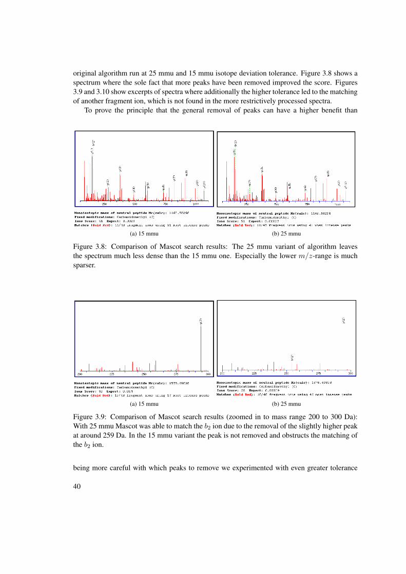
original algorithm run at 25 mmu and 15 mmu isotope deviation tolerance. Figure 3.8 shows aspectrum where the sole fact that more peaks have been removed improved the score. Figures3.9 and 3.10 show excerpts of spectra where additionally the higher tolerance led to the matchingof another fragment ion, which is not found in the more restrictively processed spectra.
To prove the principle that the general removal of peaks can have a higher benefit than
(a) 15 mmu (b) 25 mmu
Figure 3.8: Comparison of Mascot search results: The 25 mmu variant of algorithm leavesthe spectrum much less dense than the 15 mmu one. Especially the lower m/z-range is muchsparser.
(a) 15 mmu (b) 25 mmu
Figure 3.9: Comparison of Mascot search results (zoomed in to mass range 200 to 300 Da):With 25 mmu Mascot was able to match the b2 ion due to the removal of the slightly higher peakat around 259 Da. In the 15 mmu variant the peak is not removed and obstructs the matching ofthe b2 ion.
being more careful with which peaks to remove we experimented with even greater tolerance
40
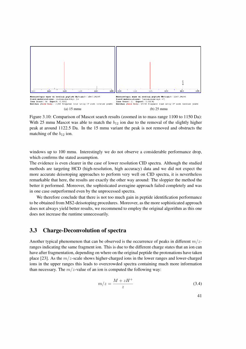
(a) 15 mmu (b) 25 mmu
Figure 3.10: Comparison of Mascot search results (zoomed in to mass range 1100 to 1150 Da):With 25 mmu Mascot was able to match the b12 ion due to the removal of the slightly higherpeak at around 1122.5 Da. In the 15 mmu variant the peak is not removed and obstructs thematching of the b12 ion.
windows up to 100 mmu. Interestingly we do not observe a considerable performance drop,which confirms the stated assumption.The evidence is even clearer in the case of lower resolution CID spectra. Although the studiedmethods are targeting HCD (high-resolution, high accuracy) data and we did not expect themore accurate deisotoping approaches to perform very well on CID spectra, it is neverthelessremarkable that here, the results are exactly the other way around: The sloppier the method thebetter it performed. Moreover, the sophisticated averagine approach failed completely and wasin one case outperformed even by the unprocessed spectra.
We therefore conclude that there is not too much gain in peptide identification performanceto be obtained from MS2-deisotoping procedures. Moreover, as the more sophisticated approachdoes not always yield better results, we recommend to employ the original algorithm as this onedoes not increase the runtime unnecessarily.
3.3 Charge-Deconvolution of spectra
Another typical phenomenon that can be observed is the occurrence of peaks in different m/z-ranges indicating the same fragment ion. This is due to the different charge states that an ion canhave after fragmentation, depending on where on the original peptide the protonations have takenplace [23]. As the m/z-scale shows higher-charged ions in the lower ranges and lower-chargedions in the upper ranges this leads to overcrowded spectra containing much more informationthan necessary. The m/z-value of an ion is computed the following way:
m/z =M + zH+
z(3.4)
41

Algorithm 3.2: Charge-Deconvolution as implemented by Savitski et al. [38]Input : A list of (pos, I)-pairs, peaks, of length N ascendingly ordered by pos
Structure containing precursor ion information, precursorOutput: Charge-deconvolved peaks list
1 p← 1.007276; // molecular mass of a proton2 for i← 1 to N do3 if peaks[i].z > 1 then4 peaks [i].pos← peaks [i].pos ·(peaks[i].z− 1)H+ ;5 peaks [i].z = 1 ;6 end7 end
whereM is the molecular mass of the ion, z its charge state andH+ the mass of a proton, whichis ca. 1.007276 Da.E.g., if a fragment having the molecular mass of 1500 Da would occur singly-, doubly- andtriply-charged, the respective spectra would contain peaks at 1500 Da, 751 Da and 501 Da,respectively.
Most search engines do not consider higher charged ions (Mascot, for example, only consid-ers singly- and doubly-charged fragment ions) as this would exponentially increase the searchspace. Therefore it seems a promising approach to remove multiply-charged replicas of the samefragment ion from the spectra and only keep the singly-charged ones.
Clearly, for charge-deconvolution to be possible, the charge states of the peaks have to beknown. It is therefore recommended to perform the Deisotoping procedure beforehand, if thepeaks in the spectra are not annotated with charge states or it is unclear if they are.
3.3.1 A simple Charge-Deconvolution algorithm
For the charge-deconvolution we followed the same approach as for the deisotoping. We startedfrom the existing algorithm developed for H-Score [38].The principle of the algorithm is quite simple. For the charge-deconvolution only one simpleiteration through the peak-list is necessary. For each peak with a charge state greater than 1 thesingly-charged m/z-value is then calculated according to eq. 3.4:
msc = m/z · (z − 1)H+ (3.5)
The peak is then simply replaced by a new peak at positionmsc having the same intensity but thecharge state z = 1. Algorithm 3.2 illustrates this procedure. Unfortunately, the preprocessingwith this method only yields a negligible improvement in the identification performance (seesection 5.2). Here, two possible problems play a role:
1. The “conversion” of a peak indicating a multiply-charged ion into a peak indicating asingly-charged peak does not take into consideration, if there already is a peak for the
42

singly-charged ion. As a possibly already existing peak will in general not have exactlythe same m/z-value as the shifted one, this will lead to peaks referring to the same ionwhich are, from the search engine’s point of view, competing with each other. This willhowever, lower the resulting score for matched peaks in the same m/z-range.
2. Even though the charge-deconvolution thins out the lower m/z-regions where the peaksof the multiply-charged ions can be found the higher regions are populated with additionalpeaks, which leads to new competing peaks there. The obtained benefits from the thin-ning might therefore just be canceled out by the suffered score decrease through the newcompeting peaks.
Although the second problem clearly cannot be eliminated we experimented how the algorithmperforms, if the search engine only considers singly-charged ions.Here, we do observe a greater increase in PSMs, however the improvement can still not beconsidered significant and, in particular, it is lower than having the search engine make use ofthe doubly-charged ions.
Furthermore, we tried to reduce the negative effect of newly introduced peaks by consolidat-ing an already existing peak with the shifted one, i.e. by solving the first problem. To achievethis we changed the algorithm to look for an already existing peak at the position (± 0.01 Da)the converted peak would be shifted to. If such a peak exists the two peaks’ intensities are com-pared. Whichever has the higher intensity remains in the spectrum, the other one is removed.Additionally, the remaining peak’s intensity is increased by the intensity of the removed peak.This revised method is given in algorithm 3.3. In fact, this change had no effect whatsoever onthe resulting PSMs. The only measurable change was very small and only occurred for one ofour three test instances (see 5.2) that it can be considered negligible.
3.4 Results and Future Work
As a result of the analyses described in this section we decided to implement the simple existingdeisotoping and charge-deconvolution procedures in a plugin for the Proteome Discoverer soft-ware, version 1.3.0.339, by Thermo Fisher Scientific: The MS2-Spectrum Processor node, thatcan be integrated in the workflow. As there was no significant performance increase by the moresophisticated methods, we chose the simple approaches to not necessarily waste computationtime. The software allows the setting of a desired tolerance value for the deisotoping method, aswell as the general choice, if deisotoping and/or charge-deconvolution should be applied to theMS2-spectra.For testing purposes and possible analyses of spectra it is also possible to switch to the averaginemodeling approach. However, as we have showed in this section, this will not necessarily yielda higher PSM count and is therefore not recommended as a standard procedure in the process-ing workflow. Similarly, we implemented the modified charge-deconvolution method for testingpurposes, as we believe it is more exact than the original one.
As the more sophisticated algorithms did not yield significant improvements in comparisonto the simple algorithm we assume that the design of even more complex methods would prob-ably also not be very promising. The final algorithms implemented in the plugin are therefore
43

Algorithm 3.3: Modified Charge-Deconvolution algorithmInput : A list of (pos, I)-pairs, peaks, of length N ascendingly ordered by pos
Structure containing precursor ion information, precursorOutput: Charge-deconvolved peaks list
1 p← 1.007276; // molecular mass of a proton2 for i← 1 to N do3 if peaks[i].z > 1 then4 Msingly ← peaks [i].pos ·(peaks[i].z− 1)H+ ;5 singlyChargedPeakcur ← FindClosestPeak (Msingly) ;6 if Abs (singlyChargedPeakcur- Msingly) ≤ 0.01 then7 if peaks[i].I > singlyChargedPeakcur .I then8 peaks[i].pos = Msingly ;9 peaks[i].I = peaks[i].I + singlyChargedPeakcur .I ;
10 peaks[i].z = 1 ;11 singlyChargedPeakcur .I = 0 ;12 end13 else14 singlyChargedPeakcur .I = peaks[i].I + singlyChargedPeakcur .I ;15 peaks[i].I = 0 ;16 end17 end18 end19 else20 peaks[i].pos← peaks[i].pos · (peaks[i].z− 1)H+ ;21 peaks[i].z = 1 ;22 end23 end
24 foreach peak p in peaks do25 if p.I = 0 then26 Remove p from peaks27 end28 end
simple and not very time consuming, such that they can be generally applied in the workflowwithout having to consider excess runtime or memory limitations.
Naturally, there are many more spectrum-manipulation approaches one could apply, yet,as we demonstrated in this section, the main benefit with current search engines lies in theremoval of peaks. To this end, another possibility would be the removal of neutral loss3 peaks
3The term neutral loss describes the loss of an uncharged compound like water or ammonia, which is reflectedin the spectrum by another peak of specific m/z-offset from the original fragment ion.
44

of “confirmed” ions, i.e. ions for which an isotope pattern has been found. Furthermore, webelieve that a noise filtering method that clears the low-intensity areas of the spectrum wouldalso increase the number of PSMs.Probably another promising approach is the recalibration of MS2-spectra. For this approach atwo-searches strategy would have to be implemented where the first search generates a resultlist that serves as an input to recalibrate MS2-spectra using high-confidence identifications. Therecalibrated spectra can then be submitted to the second, actual, search. Section 4.4 describesthis idea with respect to precursor recalibration. However, for this approach to work a searchengine would be needed that rewards accurate fragment ions.
45


CHAPTER 4Precursor Precision Improvement
4.1 Motivation
In general, mass spectrometers have to take decisions on which precursor to pick for fragmenta-tion analysis within a few milliseconds. Moreover there is no spare computation time left to lookback at the chosen precursors and try to get some additional information about them. Therefore,the typical approach is to take the data that is available at the moment of the precursor-picking.However, using not only the information from the MS1-spectrum the precursor originated frombut also from other spectra in which the precursor can be found should allow for a more exactcalculation of the precursor mass.The reason is simple. As we are dealing with measured values which are subject to errors wecan model the set of all measurements of a single precursor mass by a normal distribution whosemean is the correct value of the mass. And clearly, the obtained result of averaging multiplemeasurements will, in general, be closer to the correct value than simply considering just onesingle measurement. This is even more true for spectra obtained by HCD. As described in sec-tion 2.2.4.1 these spectra feature high mass accuracy and resolution.
We thus have developed a method that can be applied as an intermediate processing step afterthe acquisition of the spectra and before the spectra are submitted to the database search engine.This way, the necessary data can be gathered from the complete raw file, i.e. all (MS1-) spectrathat have been recorded can be incorporated in the analysis, without being subject to real-timeconstraints the instrument software has to deal with when choosing precursor ions for fragmen-tation. The algorithm processes one MS2-spectrum after another with the basic input being -besides the possibility to access all raw data generated from the respective sample - the m/z-value of the precursor ion associated with the spectrum. After running the algorithm a new, morereliable m/z-value is the expected output and replaces the value originally associated with theMS2-spectrum.
47

4.2 Method
4.2.1 Basic Principle: 3d-Peaks
The key idea behind the developed approach is the 3d-peak. This concept has already beensuccessfully applied in the MaxQuant software and it has been shown that the number of pep-tide identifications could be increased dramatically [7]. However, the proposed algorithm doesnot always extract 3d-peaks correctly and tends to be too restrictive. Furthermore, we employdifferent methods of improving the precision of the resulting m/z-value, as a part of the massimprovement employed in MaxQuant is based on the detection of SILAC pairs or triplets 1,which cannot be applied in general, i.e. for non-labeled samples. Last but not least, the algo-rithm in MaxQuant has been developed and tested for CID spectra, for HCD spectra differentapproaches might be necessary.Nonetheless, the general concept of 3d-peaks promised to serve as a solid basis for the develop-ment of our algorithm.
As described above the aim is to collect further precursor data from different MS1-spectrathan the one the precursor ion was selected from. The logical step to take is therefore to studyprecursor peaks not only in the m/z-intensity plane but to include the retention time as the thirddimension and consider three-dimensional peaks.The basic method for 3-dimensional peak-picking is simple:
1. Search the precursor in the original MS1-spectrum and gather its profile points.
2. Starting from this spectrum, traverse backwards through the MS1-spectra and search forthe current precursor in each of them, until the precursor cannot be found anymore.
3. Starting from this spectrum, traverse forwards through the MS1-spectra and search for thecurrent precursor in each of them, until the precursor cannot be found anymore.
⇒ The 3d-peak is constructed from the separate 2d-peaks formed by the profile points that wereobtained from the respective MS1-spectra.In the following, we will refer to the peak formed by the profile points as a 2d-peak, while the“peak” obtained by regarding the sequence of the 2d-peaks is referred to as the 3d-peak. Figure4.1 illustrates the connection between 2d- and 3d-peaks.
Although the basic idea behind the algorithm sounds simple, especially the construction ofthe 3d-peak and the decision where the peak ends is a complex problem, which will becomeclear in sections of this chapter.The details of the algorithm are described in the following.
4.2.1.1 2d-Peak Detection
The first basic element of the algorithm is the detection of a 2d-peak in a single MS1-spectrum.Recall that a 2d-peak is defined by the profile points of which there are around 10,000 to 20,000
1SILAC is a method of quantitative proteomics, in which peptides are labeled with light and heavy forms of acertain amino acid. Based on this labeling the measured peptides can then be quantified.
48

Figure 4.1: a) A 2d-peak formed by the profile points in a specific MS1-spectrum. The greenline depicts the centroid of the peak, the two red lines define its ends. b) A 3d-peak composedof five 2d-peaks that were found in different MS1-scans adjacent to each other [7].
in an average MS1-spectrum, depending on the resolution. The challenge is therefore to collectonly the profile points that are in fact part of the same peak. As the peak shapes are usuallyGaussian, the peaks can be separated very confidently from each other leading to a very simplemethod to collect exactly the profile points that form one peak. Starting from the profile pointclosest to the expected centroid value, the list of profile points is traversed both towards lowerand higher m/z regions until a point is reached whose intensity value is 0 or a local intensityminimum was detected, indicating a so-called split peak. Note that the former criterion can beapplied since on the edges of the peaks there are usually several profile points with intensity 0included in the list. This is due to the baseline- and noise-filtering applied by the instrumentsoftware while writing the data to the raw file. If this were not the case, and only peak data werestored in the list, the two neighboring peaks could still be separated via the second criterion. Anexample of where a split peak would be detected can be seen in Figure 4.2. Naturally, whensearching for the point closest to the given centroid, a tolerance window around this centroid hasto be applied, s.t. cases where there is no point inside the window result in no matching peak. Agood choice is a window width of 5 to 10 ppm.It was proposed that this simple approach of detecting the 2d-peak is sufficient for spectrarecorded by high precision instruments [7].
After the profile points of a peak have been collected, its centroid is calculated. As the peakshape is Gaussian it is an accurate approach to fit a Gaussian function to the collected profile
49

Figure 4.2: Example of a 2d-split peak: Note that the margin between the two bordering peakscan easily be found by searching for the local minimum [7].
points and to determine the centroid of this function. In their supplemental material Cox etal. [7] suggest the following formula to calculate an approximation of the centroidm a Gaussianfunction fitted to the profile points would have
m =1
2
(L0 − L1)m2−1 + (L1 − L−1)m
20 + (L−1 − L0)m
21
(L0 − L1)m−1 + (L1 − L−1)m0 + (L−1 − L0)m1(4.1)
where m−1,m0, m1 are the m/z-values (i.e. the positions) of the three central profile points,and L−1, L0, L1 are the natural logarithms of the corresponding intensities. For the rare casesthat a peak is defined by less than two profile points the centroid is given by the average of theirm/z-values weighted by their intensities.
A closer analysis of this formula confirms that it can indeed be used to determine the centroidof a Gaussian. The general Gaussian function is defined by
f(x) = ae−(x−b)2
2c2 (4.2)
where a, b, c > 0.Applying the natural logarithm to this function yields a quadratic function
lnf(x) = ln a− 1
2c2x2 +
b
c2x− b2
2c2(4.3)
which in its general form is given by
lnf(x) = ax2 + bx+ c (4.4)
Now, in our case the domain of this parabola ism/z and the function range are the logarithmizedintensities. We can determine the three unknown coefficients, a, b and c of the function bysolving a system of three linear equations using the given three m/z-values m−1,m0,m1, andthe corresponding logarithmized intensities L−1, L0, L1.
L−1 = a m2−1 + b m−1 + c (4.5)
L0 = a m20 + b m0 + c (4.6)
L1 = a m21 + b m1 + c (4.7)
50

Note that the centroid of a parabola is equal to its maximum, which can easily be obtained bydifferentiation, i.e. m can be found by solving
m = − b
2a(4.8)
The constant part of the function c, is therefore irrelevant and we can proceed in the followingway:By subtracting 4.7 from 4.6, 4.5 from 4.7 and 4.6 from 4.5 we obtain
L0 − L1 = a(m20 −m2
1) + b(m0 −m1) (4.9)
L1 − L−1 = a(m21 −m2
−1) + b(m1 −m−1) (4.10)
L−1 − L0 = a(m2−1 −m2
0) + b(m−1 −m0) (4.11)
Now, we divide 4.9 by (m0−m1), 4.10 by (m1−m−1) and 4.10 by (m−1−m0) which yields
L0 − L1
(m0 −m1)= a(m0 +m1) + b (4.12)
L1 − L−1
(m1 −m−1)= a(m1 +m−1) + b (4.13)
L−1 − L0
(m−1 −m0)= a(m−1 +m0) + b (4.14)
In order to isolate a, we subtract 4.13 from 4.12:
L0 − L1
(m0 −m1)− L1 − L−1
(m1 −m−1)= a(m0 −m−1)
a =L0 − L1
(m0 −m1) · (m0 −m−1)− L1 − L−1
(m1 −m−1) · (m0 −m−1)
=(L0 − L1) · (m1 −m−1)− (L1 − L−1) · (m0 −m1)
(m0 −m1) · (m1 −m−1) · (m0 −m−1)
=(L1 − L0)m−1 + (L−1 − L1)m0 + (L0 − L−1)m1
(m0 −m1) · (m1 −m−1) · (m0 −m−1)(4.15)
Now, we use equation 4.14 in order to isolate b
b =L−1 − L0
(m−1 −m0)− a(m−1 +m0) (4.16)
and insert a as calculated above:
b =L−1 − L0
(m−1 −m0)− (m−1 +m0) · ((L1 − L0)m−1 + (L−1 − L1)m0 + (L0 − L−1)m1)
(m0 −m1) · (m1 −m−1) · (m0 −m−1)
=(L−1 − L0) · (m0 −m1) · (m1 −m−1) · (m0 −m−1)
(m−1 −m0) · (m0 −m1) · (m1 −m−1) · (m0 −m−1)
−(m2
−1 −m20) · ((L1 − L0)m−1 + (L−1 − L1)m0 + (L0 − L−1)m1)
(m−1 −m0) · (m0 −m1) · (m1 −m−1) · (m0 −m−1)
51

=(L−1 − L0) · (m−1 −m1) · (m0 −m1)
(m0 −m1) · (m1 −m−1) · (m0 −m−1)
−(m−1 +m0) · ((L1 − L0)m−1 + (L−1 − L1)m0 + (L0 − L−1)m1)
(m0 −m1) · (m1 −m−1) · (m0 −m−1)
=(L0 − L1)m
2−1 + (L1 − L−1)m
20 + (L−1 − L0)m
21
(m0 −m1) · (m1 −m−1) · (m0 −m−1)(4.17)
Finally, a and b can be inserted into the derivative, 4.8:
1
2
(L0 − L1)m2−1 + (L1 − L−1)m
20 + (L−1 − L0)m
21
(L0 − L1)m−1 + (L1 − L−1)m0 + (L−1 − L0)m1(4.18)
which is exactly the proposed formula.We conclude that the proposed formula indeed yields the centroid of a fitted Gaussian to the
three profile points.The intensity of a 2d-peak is given by the area under the Gaussian curve. However, be-
cause the intervals between the separate profile points are nearly constant, the total intensity, i.e.sum of the separate intensities is proportional to the area under the Gaussian [7]. For furthercomputations the centroid-m/z and the total intensity are stored for the each 2d-peak.
It is therefore possible to obtain reasonably good approximations of the centroid and theintensity of a Gaussian peak without actually performing a runtime-expensive linear regressionof a Gaussian function to the profile points.
Note that this is also done for the original precursor m/z received as input, as we want tomake sure that the centroid, that is being used further on by the algorithm is from that 2d-peakonly. As the instruments apply a proprietary peak-picking algorithm it is not clear how theoriginal centroid value has been calculated.
4.2.1.2 3d-Peak Centroid
After calculating the centroid for each 2d-peak the actually sought 3d-peak centroid is calcu-lated. This is done by simply computing the average of the n 2d-peak centroids (mi, 1 ≤ i ≤ n)weighted by the corresponding total intensities (Ii, 1 ≤ i ≤ n):
m/z3d =
∑ni=1miIi∑ni=1 Ii
(4.19)
This is the value that is output by the algorithm replacing the original precursor m/z-value.The idea behind this calculation is the fact that the measured values become less accurate
the closer the intensity is to the (technical) noise level. Therefore, the higher confidence inm/z-values stemming from highly intense peaks is expressed by the greater weight.
4.3 3d-Peak Reconstruction
A crucial aspect of the algorithm has not been discussed yet: How is a 3d-peak constructed?Since the retention time dimension of the 3d-peak should reflect the elution behavior of the
52
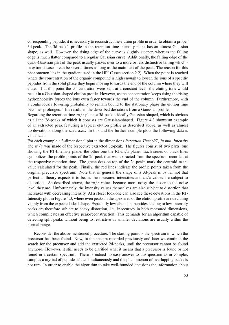
corresponding peptide, it is necessary to reconstruct the elution profile in order to obtain a proper3d-peak. The 3d-peak’s profile in the retention time-intensity plane has an almost Gaussianshape, as well. However, the rising edge of the curve is slightly steeper, whereas the fallingedge is much flatter compared to a regular Gaussian curve. Additionally, the falling edge of thequasi-Gaussian part of the peak usually passes over to a more or less distinctive tailing which -in extreme cases - can be several times as long as the main part of the peak. The reason for thisphenomenon lies in the gradient used in the HPLC (see section 2.2). When the point is reachedwhere the concentration of the organic compound is high enough to loosen the ions of a specificpeptides from the solid phase they begin moving towards the end of the column where they willelute. If at this point the concentration were kept at a constant level, the eluting ions wouldresult in a Gaussian-shaped elution profile. However, as the concentration keeps rising the risinghydrophobicity forces the ions even faster towards the end of the column. Furthermore, witha continuously lowering probability to remain bound to the stationary phase the elution timebecomes prolonged. This results in the described deviations from a Gaussian profile.Regarding the retention time-m/z plane, a 3d-peak is ideally Gaussian-shaped, which is obviousas all the 2d-peaks of which it consists are Gaussian-shaped. Figure 4.3 shows an exampleof an extracted peak featuring a typical elution profile as described above, as well as almostno deviations along the m/z-axis. In this and the further example plots the following data isvisualized:For each example a 3-dimensional plot in the dimensions Retention Time (RT) in min, Intensityand m/z was made of the respective extracted 3d-peak. The figures consist of two parts, oneshowing the RT-Intensity plane, the other one the RT-m/z plane. Each series of black linessymbolizes the profile points of the 2d-peak that was extracted from the spectrum recorded atthe respective retention time. The green dots on top of the 2d-peaks mark the centroid m/z-value calculated for the peak. Finally, the red lines indicate the profile points taken from theoriginal precursor spectrum. Note that in general the shape of a 3d-peak is by far not thatperfect as theory expects it to be, as the measured intensities and m/z-values are subject todistortion. As described above, the m/z-values become more noisy the closer to the noiselevel they are. Unfortunately, the intensity values themselves are also subject to distortion thatincreases with decreasing intensity. At a closer look one can also see these deviations in the RT-Intensity plot in Figure 4.3, where even peaks in the apex area of the elution profile are deviatingvisibly from the expected ideal shape. Especially low-abundant peptides leading to low-intensitypeaks are therefore subject to heavy distortion, i.e. inaccuracy in both measured dimensions,which complicates an effective peak-reconstruction. This demands for an algorithm capable ofdetecting split peaks without being to restrictive as smaller deviations are usually within thenormal range.
Reconsider the above-mentioned procedure. The starting point is the spectrum in which theprecursor has been found. Now, in the spectra recorded previously and later we continue thesearch for the precursor and add the extracted 2d-peaks, until the precursor cannot be foundanymore. However, it still needs to be clarified what it means that a precursor is found or notfound in a certain spectrum. There is indeed no easy answer to this question as in complexsamples a myriad of peptides elute simultaneously and the phenomenon of overlapping peaks isnot rare. In order to enable the algorithm to take well-founded decisions the information about
53
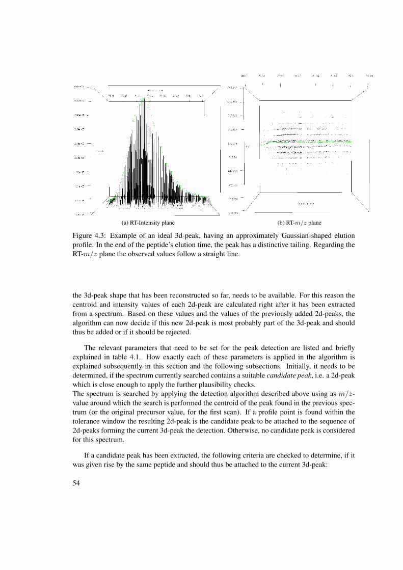
(a) RT-Intensity plane (b) RT-m/z plane
Figure 4.3: Example of an ideal 3d-peak, having an approximately Gaussian-shaped elutionprofile. In the end of the peptide’s elution time, the peak has a distinctive tailing. Regarding theRT-m/z plane the observed values follow a straight line.
the 3d-peak shape that has been reconstructed so far, needs to be available. For this reason thecentroid and intensity values of each 2d-peak are calculated right after it has been extractedfrom a spectrum. Based on these values and the values of the previously added 2d-peaks, thealgorithm can now decide if this new 2d-peak is most probably part of the 3d-peak and shouldthus be added or if it should be rejected.
The relevant parameters that need to be set for the peak detection are listed and brieflyexplained in table 4.1. How exactly each of these parameters is applied in the algorithm isexplained subsequently in this section and the following subsections. Initially, it needs to bedetermined, if the spectrum currently searched contains a suitable candidate peak, i.e. a 2d-peakwhich is close enough to apply the further plausibility checks.The spectrum is searched by applying the detection algorithm described above using as m/z-value around which the search is performed the centroid of the peak found in the previous spec-trum (or the original precursor value, for the first scan). If a profile point is found within thetolerance window the resulting 2d-peak is the candidate peak to be attached to the sequence of2d-peaks forming the current 3d-peak the detection. Otherwise, no candidate peak is consideredfor this spectrum.
If a candidate peak has been extracted, the following criteria are checked to determine, if itwas given rise by the same peptide and should thus be attached to the current 3d-peak:
54

Name Data Type Abbreviation DescriptionTolerance double tol Defines the maximal deviation from the
original centroid. I.e. a tolerance win-dow of±tol is applied around the orig-inal centroid.
Minimum ProfilePoints
int nmin A candidate peak needs at least nmin
profile points in order to be considered.Skip Scans int skip The amount of spectra that can be
skipped in case the candidate peak doesnot match the criteria.
Points for Regres-sion
int nreg The amount of 2d-peaks that are takeninto account for the linear regressionused in peak-profile tracking.
Points for MassDrift Detection
int ndrift The amount of 2d-peaks that are takeninto account for the detection of slowmass drifts.
Table 4.1: 3d-peak reconstruction: Relevant settings
4.3.1 Minimum Profile Points in 2d-Peak
If the extracted candidate peak does not consist of more than the set minimum amount of profilepoints it is rejected. The reason is that due to noise- and baseline-correction performed by themass spectrometer the extracted peak represents only the apex region of the actual peak. Con-sequently, the m/z-values of the remaining profile points, and moreover the centroid, will mostprobably not be very accurate.One might argue that the part such a very low intense peak will contribute to the weighted-average centroid of the 3d-peak is insignificant, which is certainly true. This check is never-theless valuable as every increase in precision - no matter how small - can be an advantage.Additionally, this check rather reduces than increases the runtime of the algorithm. When thepeak reconstruction reaches the margins of the 3d-peak, the 2d-peaks clearly become less in-tense. This means that as soon as a 2d-peak is encountered, that is so small that it no longerconsists of a high enough amount of profile points, the 3d-peak is already ending. It is thereforereasonable to stop the search and not to continue until no 2d-peak at all can be found anymore.This is especially true in the tailing area of the 3d-peak, where there can still be plenty of spectracontaining a low intense 2d-peak that is, strictly seen, part of the same 3d-peak. Added up thesepeaks’ intensities could have a considerable amount of weight to observably alter the overallcentroid.In the light of these considerations this criterion becomes much more valuable as it appears at afirst glance.
55
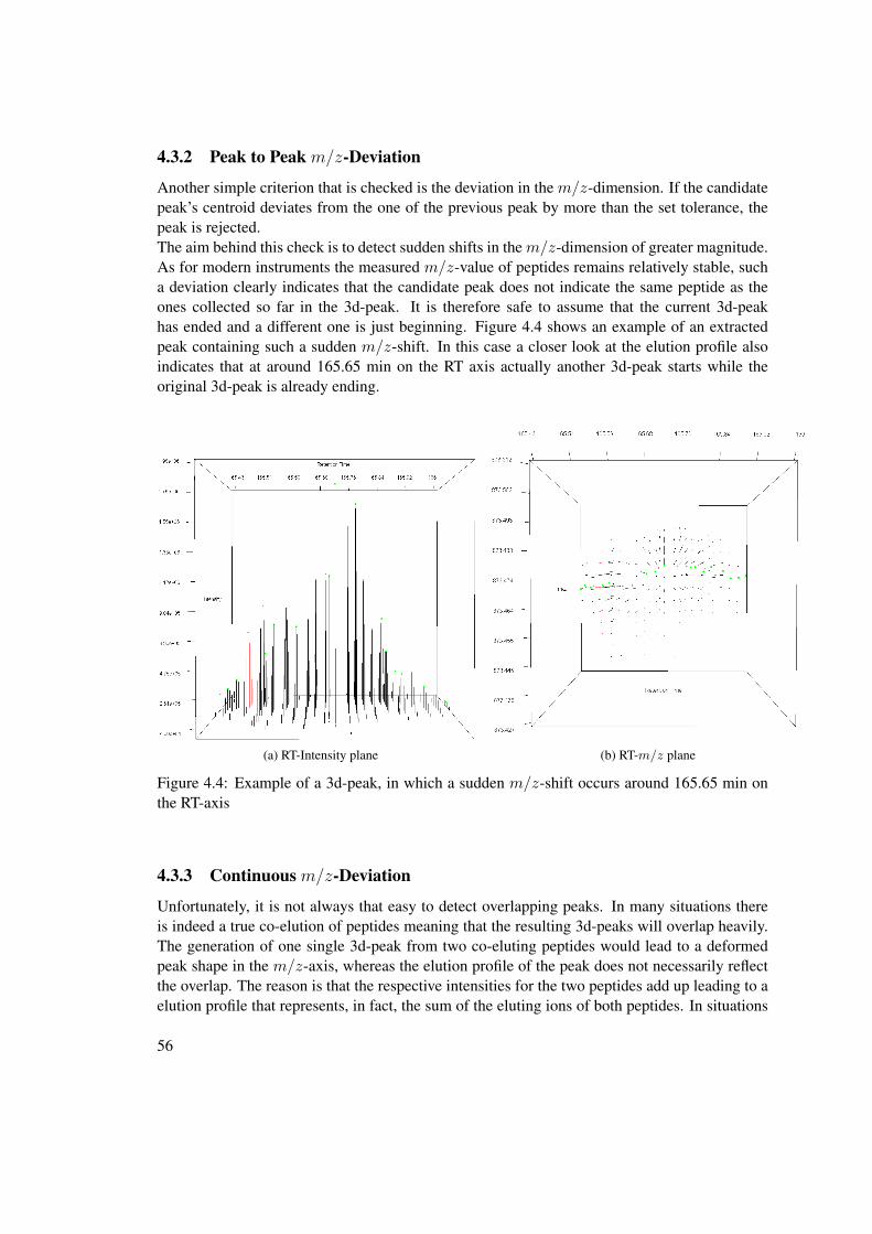
4.3.2 Peak to Peak m/z-Deviation
Another simple criterion that is checked is the deviation in the m/z-dimension. If the candidatepeak’s centroid deviates from the one of the previous peak by more than the set tolerance, thepeak is rejected.The aim behind this check is to detect sudden shifts in them/z-dimension of greater magnitude.As for modern instruments the measured m/z-value of peptides remains relatively stable, sucha deviation clearly indicates that the candidate peak does not indicate the same peptide as theones collected so far in the 3d-peak. It is therefore safe to assume that the current 3d-peakhas ended and a different one is just beginning. Figure 4.4 shows an example of an extractedpeak containing such a sudden m/z-shift. In this case a closer look at the elution profile alsoindicates that at around 165.65 min on the RT axis actually another 3d-peak starts while theoriginal 3d-peak is already ending.
(a) RT-Intensity plane (b) RT-m/z plane
Figure 4.4: Example of a 3d-peak, in which a sudden m/z-shift occurs around 165.65 min onthe RT-axis
4.3.3 Continuous m/z-Deviation
Unfortunately, it is not always that easy to detect overlapping peaks. In many situations thereis indeed a true co-elution of peptides meaning that the resulting 3d-peaks will overlap heavily.The generation of one single 3d-peak from two co-eluting peptides would lead to a deformedpeak shape in the m/z-axis, whereas the elution profile of the peak does not necessarily reflectthe overlap. The reason is that the respective intensities for the two peptides add up leading to aelution profile that represents, in fact, the sum of the eluting ions of both peptides. In situations
56

where the overlap is big, one does not even observe abrupt mass shifts, as a big overlap meansthat the profile points of both peptides overlap in many spectra leading to many joint 2d-peaks.Therefore the respective centroids of these peaks only gradually drift from them/z-range of onepeptide, to the other one. Figure 4.5 shows an example of a 3d-peak whose m/z axis contains acontinuous drift upwards. One could assume by inspecting the elution profile that there are twopeaks, the first one ending at around 116.9 min, the second one starting at around 116.75 min.Thus, 5 to 6 2d-peaks are overlapping, which is reflected in the m/z-drift, which ranges overthe said 5 to 6 2d-peaks.
For the sake of detecting such drifts the algorithm analyzes a number of previous 2d-peaks
(a) RT-Intensity plane (b) RT-m/z plane
Figure 4.5: Example of 3d-peak, in which a continuous m/z-drift occurs. Note that by inspect-ing solely the elution profile one can only assume but not with certainty conclude that the peakin fact indicates the presence of two peptides.
(according to the set points to use for the mass drift detection) plus the candidate peak. If intotal the m/z-deviation between the consecutive peaks is greater than the tolerance thresholdthe candidate peak is rejected.
4.3.4 Elution Profile Tracking
There are also situations in which the shape of the elution profile can give a hint where a 3d-peakshould end, while the inspection of the RT-m/z plane might not allow this conclusion. Figure4.6 shows an example of such a peak. Whereas in the elution profile the incision between thetwo peaks is clearly visible, the m/z-value only deviates slightly between consecutive peaks.The masses of the peptides are too close to each other, s.t. these deviations are well within theexpected inaccuracy due to technical noise.
57

Because of the normal deviations in the elution profile it is not possible to apply a method as
(a) RT-Intensity plane (b) RT-m/z plane
Figure 4.6: Example of 3d-peak split peak. Note that although the incision is obvious in the RT-Intensity plane, the deviations visible in the RT-m/z plane are not conclusive enough to detectit.
simple as in the 2d-peak extraction scenario. The general idea of tracking the slope of the profileis nevertheless a suitable way of detecting the margins of a peak. As an approach capable ofcompensating these fluctuations we choose to take the intensities of a defined number nreg − 1of previous 2d-peaks, plus the intensity of the candidate peak, into account. Given the retentiontimes RTi of the 2d-peaks and the and the corresponding intensities Ii, for 1 ≤ i ≤ nreg, weperform a linear regression in order to fit a straight line through the data. The slope from theobtained line can then be used as an indicator in the same way as in the 2d-peak setting. I.e. theslope is traced to detect local minima, which most probably indicate the end of the peak.
Finally, to further compensate for possible inaccuracies in the measurements which can leadto unpredictable deviations in the data the algorithm may always skip one spectrum, in which nosuitable candidate peak was found or for which the extracted candidate peak did not pass all ofthe mentioned quality criteria. In this case, the algorithm continues with the next spectrum, as ifthe skipped one did not exist.Note that although it is possible to change this setting to allow even more spectra to be skipped,it is not recommended to do so.
58
4.3.5 Evaluation of the extracted peak
The described quality criteria for the 3d-peak reconstruction are chosen to detect the marginsof the peak but not to be too restrictive. However, experiments have shown, that some of theextracted peaks are still obviously incorrect. The algorithm still fails to detect split peaks whenthe overlap between the two respective peaks is too high. Figure 4.7 shows an example of anobvious split peak which has not been separated by the algorithm. Inspection of the RT-Intensityplane by eye would suggest the conclusion that these are actually two peaks. In the RT-m/zplane the situation is even more obvious. Here the drawback of the decision to design thealgorithm in a not too restrictive way becomes apparent.
(a) RT-Intensity plane (b) RT-m/z plane
Figure 4.7: Example of 3d-peak split peak that could not be detected by the algorithm. Note thatalthough the deviations in both measured dimensions strongly indicate a split peak, the algorithmis too less restrictive to detect it.
Therefore, a final evaluation is done after the peak has been reconstructed. For detectingsuch split peak the following steps are performed:
• Smooth the n centroid values of the 2d-peaks by applying a 5-point average filter, resultingin n− 4 smoothed centroids: cs0, . . . c
sn−4.
• Excluding cs0 and csn−4: Determine the range within each 5 consecutive points, i.e. theminimal and maximal m/z value: csmin and csmax
• If csmax − csmin ≥ 4 ppm: Reject the 3d-peak altogether.
The idea behind this check is to detect unusual mass shifts in a central area of the peak. Inprincipal, the same concept is followed as for the constant checking of them/z-deviations during
59
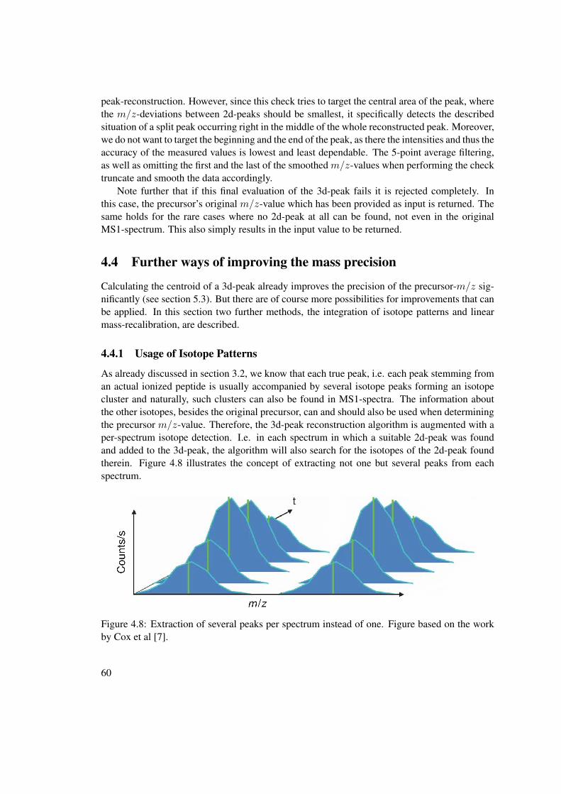
peak-reconstruction. However, since this check tries to target the central area of the peak, wherethe m/z-deviations between 2d-peaks should be smallest, it specifically detects the describedsituation of a split peak occurring right in the middle of the whole reconstructed peak. Moreover,we do not want to target the beginning and the end of the peak, as there the intensities and thus theaccuracy of the measured values is lowest and least dependable. The 5-point average filtering,as well as omitting the first and the last of the smoothed m/z-values when performing the checktruncate and smooth the data accordingly.
Note further that if this final evaluation of the 3d-peak fails it is rejected completely. Inthis case, the precursor’s original m/z-value which has been provided as input is returned. Thesame holds for the rare cases where no 2d-peak at all can be found, not even in the originalMS1-spectrum. This also simply results in the input value to be returned.
4.4 Further ways of improving the mass precision
Calculating the centroid of a 3d-peak already improves the precision of the precursor-m/z sig-nificantly (see section 5.3). But there are of course more possibilities for improvements that canbe applied. In this section two further methods, the integration of isotope patterns and linearmass-recalibration, are described.
4.4.1 Usage of Isotope Patterns
As already discussed in section 3.2, we know that each true peak, i.e. each peak stemming froman actual ionized peptide is usually accompanied by several isotope peaks forming an isotopecluster and naturally, such clusters can also be found in MS1-spectra. The information aboutthe other isotopes, besides the original precursor, can and should also be used when determiningthe precursor m/z-value. Therefore, the 3d-peak reconstruction algorithm is augmented with aper-spectrum isotope detection. I.e. in each spectrum in which a suitable 2d-peak was foundand added to the 3d-peak, the algorithm will also search for the isotopes of the 2d-peak foundtherein. Figure 4.8 illustrates the concept of extracting not one but several peaks from eachspectrum.
Figure 4.8: Extraction of several peaks per spectrum instead of one. Figure based on the workby Cox et al [7].
60

Detection of isotopes is done by searching for 2d-peak patterns following the precursor (i.e.the monoisotopic) 2d-peak where the distance between each centroid is ca. 1/z and fitting anaveragine pattern to evaluate, if the detected pattern is indeed an isotope pattern. The samealgorithm that has been developed for the MS2-spectrum manipulation based on the ratios be-tween observed and measured isotope intensities (see section 3.2) can be applied. Note thatthe charge state of the precursor is known, therefore there is only one possible isotope pattern.The averagine-test is therefore rather a check for unperturbed data than if the detected patternis indeed an isotope pattern. Should the pattern fit well enough, we additionally consider the1 13C, 2 13C and 3 13C. Further isotope peaks are not considered as they are, if visible at all, tooless intense to provide exact uperturbed data. This is due to the usual mass range for peptides inshotgun proteomics experiments, which is between 300 and 3000 Da. See Figure 3.3 in section3.2, which illustrates these circumstances.
Of course, the obtained centroid values need to be calculated back to the monoisotopic 2d-peak, which is done by simply subtracting a neutron for the 1 13C isotope, two for the 2 13Cisotope, etc. The centroid values of the additionally acquired 2d-peaks are then also added in thefinal calculation (eq. 4.19) which computes the centroid by weighted averaging of the 2d-peaks’intensities.From a statistical point of view the integration of even more 2d-peaks in this equation shouldfurther increase the precision of the precursor mass.
4.4.2 Linear Mass Recalibration
The algorithm described so far improves the MS1 precursor precision by extracting and evalu-ating data from the respective .raw-file and can thus in principle be applied offline and separatefrom any workflow. The method described in the following needs to be integrated in a workflow.The basic idea to this approach has already been proposed by Cox et al. [7] who perform a re-calibration of the precursor masses obtained in the search results. Using high-scoring peptides,an average of their deviations in ppm from the theoretical masses is calculated. Subsequently,this value is subtracted from all the precursor masses.Cox et al., in fact, also published a much more complex method for recalibration [8]. However,their intention was mainly to replace the lock mass, a hardware mechanism used by the instru-ment to internally correct mass shifts over time. This method basically performs a recalibrationof the m/z-values in two dimensions, retention time and m/z.
Since we rely on a working lock mass calibration, which performs the correction of themass shift over the retention time dimension, we only use one dimension: m/z. Moreover, themanual analysis of several datasets suggested a polynomial of degree 3 as the most suitable fitstill avoiding overfitting of the data.The procedure therefore looks as follows:
1. Perform a search with relaxed search parameters in order to quickly obtain a rough searchresult.
2. Filter the result list for peptides that have a search engine rank of 1, minimum length of 8and a score that is among the top 5% scores of these peptides.
61

3. Determine the (m/z, ppm deviation)-pairs for the filtered peptides.
4. Fit a polynomial of degree 3 to this data by applying Linear-Least-Squares minimization.
5. Recalibrate all precursor m/z-values of the search input by subtracting the function valueof the polynomial at position m/z from it. This results in a ppm-value distribution aroundthe x-axis, i.e. a normalization of the ppm-errors by setting the average to 0.
Note that the first search has to be done against a normal target database that does not containany decoy sequences as the recalibration should, of course, be in favor of the target peptides.Otherwise we would introduce a bias towards the decoy peptides.Figure 4.9 shows the ppm-errors plotted against the m/z-values of high-confident peptides ofa sample dataset before and after the recalibration. The benefit of this method is to obtain anaverage ppm-error of (ideally) 0 in every m/z-range, which in turn also reduces the overallstandard deviation. It is therefore, besides the obvious benefit of drawing the average ppm-distribution around 0 and therefore increasing the precision, also necessary to make the resultscomparable by having an, in a sense, “unbiassed” standard deviation.
(a) ppm-error distribution before recalibration (b) ppm-error distribution after recalibration
Figure 4.9: Recalibration of precursor m/z-values of a sample dataset to achieve normalizationof the ppm-errors around the zero line.
4.5 Resulting Software
The proposed peak-reconstruction algorithm works with very low memory requirements as theMS1-spectra are analyzed one by one. Since the complete algorithm is always run for one spe-cific precursor mass, we can even fairly restrict the range of the MS1-spectra that is loadedinto memory to a few Daltons. Furthermore, the applied methods do not require complex cal-culations, such as the fitting of bivariate Gaussians or similar approaches. We are aware thatthe runtime could still be improved by an intelligent “alignment” of certain precursors for asimultaneous reconstruction of their elution profiles or even the principal parallelization of the
62
algorithm. However the implementation of these further features is beyond the scope of thisthesis.
The methods described in this section regarding peak-picking were integrated in the MS2-Spectrum Processor plugin for the Proteome Discoverer software by Thermo Fisher Scientific.Note, however, that the peak reconstruction can only work, if the full .raw file is provided as aninput to the workflow. Without access to the MS1-spectra the method cannot be executed.Furthermore, the mass recalibration has been incorporated in a second, separate plugin for theProteome Discoverer, the Post-Search Mass Recalibrator node. The recalibration can thus alsobe applied separately, without precedent peak-reconstruction. Figure 4.10 shows a ProteomeDiscoverer template, where both nodes are used. First the spectra are selected from the inputfiles, before the peak-reconstruction and/or spectrum cleaning algorithms are applied to them.Afterwards, a search with the Mascot search engine is started. The results are used for the recal-ibration in the Post Search Mass Recalibrator node, before the spectra with modified precursormasses are submitted to a second search. Afterwards, the results are validated and prepared forvisualization.
Since the peak-reconstruction has also been used in other projects, a separate .dll file, PeakRe-construct.dll, containing the relevant algorithms has been developed. This library provides func-tionality for the following additional software products that have been created during the workon this thesis:
1. Spectrum Analyzer: A stand-alone tool developed for the in-house analysis of .raw files.The goal of this software is to collect thorough information about the recorded spectra, aswell as the important instrument settings. The output provides helpful hints for tuning andoptimization of instrument settings for further experiments.Moreover, the output is user-definable which helps creating self-tailored analyses of thedata to obtain only the relevant information. Here, the library is used to obtain qualitycriteria of the chromatography, i.e. certain properties of the elution profile of the peptides.These are area, apex retention time, apex intensity and full width at half maximum of the3d-peaks reconstructed from the provided precursor masses.
2. PeakAnalyzer: This program is an internal module of the SimpatiQCo software suitedeveloped for the quality control of Thermo mass spectrometers and chromatographycolumns [36].PeakAnalyzer uses the library to obtain the area, apex retention time, apex intensity andfull width at half maximum of 3d-peaks reconstructed from the identified peptides that areused for the quality control analysis.
Furthermore, inspired by the work with the .raw files the SpectrumMerger has been developed.This software is a stand-alone tool used for consolidating quantification and identification spec-tra of the same precursor. The idea behind the tool is based on an approach by Köcher et al.who showed that taking two separate spectra for each precursor, one having CID, the other oneHCD as activation type, and consecutively merging the reporter ion area of the CID spectruminto the HCD spectrum generates a hybrid spectra combining the benefits of both methods. Thegenerally better quantification achieved by CID is added to the better identification of HCD [22].
63

Figure 4.10: A typical Proteome Discoverer (version 1.3.0.339) workflow using both devel-oped nodes: First the input files are defined and the MS2 spectra that should be used from theinput are selected. Then, the MS2 - Spectrum Processor performs - if desired - deisotoping,charge-deconvolution and precursor mass recalculation. The modified spectra are submitted toa Mascot search whose results are used for recalibration of the spectra by the Post Search MassRecalibrator. The recalibrated spectra are finally submitted to another Mascot search.
This tool was now designed for experimenting with further settings, by allowing automatic merg-ing of two spectra stemming from the same precursor regardless of the specific settings that havebeen used.
64

We have showed that the use of not only one but several features from the same and otherspectra can drastically improve the precision of precursor masses. Even more precision can beobtained by intelligent recalibration of the precursor masses based on confident identificationsof a first search.
Finally, the peak-reconstruction algorithm by itself has proved to be a valuable method forbeing integrated into instrument-analysis software.
65

CHAPTER 5Experimental Results
To test the implemented algorithms we used three different instances for the developed algo-rithms. Since the main focus of this thesis lies on the algorithms developed for improving theprecursor m/z-precision, the third instance is a set of three .raw files randomly picked from the72 files that were used to document the results of the MaxQuant software suite developed byCox et al [7], on whose idea the algorithm is based.The instances were chosen to have a certain variety in the samples in order to test the algorithmsunder different conditions.
Thorough separate analyses of the data were done for both the MS2-Spectrum Manipulationand the Precursor Precision Improvement methods. Finally, an analysis using the complete setof algorithms was conducted.
5.1 Experimental Setup
The following three instances were used for the evaluation of the developed methods:
1. 100ng HeLa, 3h gradient, HCD at NCE 30, isolation width 3 Da, MS1-res. 70000, MS2-res. 17500, recorded by a QExactive Orbitrap instrument.
2. 1µg HeLa, 3h gradient, HCD at NCE 35, isolation width 2 Da, MS1-res. 60000, MS2-res.7500, recorded by an LTQ Orbitrap Velos instrument.
3. 2µg HeLa, 2h gradient, CID at NCE 35, isolation width 2 Da, MS1-res. 60000, MS2-res.unknown, recorded by an LTQ Orbitrap instrument (3 .raw files).
The samples in all three instances have undergone a tryptic digest before being loaded on theHPLC column. The general setup of search parameters was the following:All searches were done using the Mascot search engine. It was searched against the human_swissprotdatabase, allowing 2 missed cleavage sites. The database was concatenated with a reversedatabase to allow for a posteriori determination of the FDR.
67

Unless stated otherwise we used a precursor mass tolerance of 10 ppm and a fragment masstolerance of 15 mmu (instance 1 and 2) or 0.5 Da (instance 3), respectively.Possible dynamic modifications were Phospho (ST), Phospho (Y) and Oxidation (M) in thecase of instances 1 and 2, and Acetyl (N-term), Oxidation (M), Label:13C(6)15N(2) (K) andLabel:13C(6)15N(4) (R) for instance 3. In all cases we added the static modification Car-bamidomethyl (C).
All search results were filtered to obtain an FDR of 1% at the PSM level according to theapproach described in section 2.2. I.e. the minimum peptide length was set to 8, only resultswith search engine rank 1 were accepted and the Mascot Ion Score was adapted until the FDRof 1% was reached.
5.2 MS2 - Spectrum Manipulation Results
This section summarizes the observations regarding the MS2 - spectrum manipulation methodsthat are described in chapter 3 of this thesis. Figures 5.1, 5.2 and 5.3 give a comparison of thePSMs obtained after using the different kinds of deisotoping and deconvolution methods. Onecan see that the maximum regarding the deisotoping tolerance lies at 15 mmu (for instances 1and 2, HCD data) and at 80 mmu (for instance 3, CID data). The averagine modeling approachyielded three different results for the three instances: In instance 1 the amount PSMs remainedalmost the same, in instance 2 we can observe an increase, and for instance 3 the results worsen.
The charge-deconvolution should only be applied if the further processing steps demandit, e.g. if the search engine can only handle singly-charged ions, in this setting its use yieldsan improvement. If doubly-charged ions are considered as well, the gain by applying charge-deconvolution is almost non-existent.For the improved charge-deconvolution method we observe that the effect is virtually non-existent. The only difference can be found in instance 1 when comparing both deconvolutionapproaches after applying deisotoping at 25 mmu tolerance. Only there we see a minimal in-crease in PSMs.
5.3 Precursor Precision Improvement Results
In this section we present the results of the application of the precursor m/z-recalculation al-gorithm. The first three figures, 5.4, 5.5 and 5.6, show the different ppm-error distributions ofthe identified peptides for the following three preprocessing methods filtered at 1% FDR and for10 ppm precursor tolerance:
• without any preprocessing
• with recalculation by peak-reconstruction and using of isotope patterns
• with additionally applying a recalibration of the precursor masses
We observe a significant reduction in the ppm-errors by applying the Precursor Recalculationmethod, which is expressed by a much narrower and sharper distribution of the ppm-error com-
68
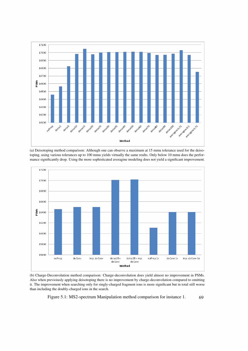
(a) Deisotoping method comparison: Although one can observe a maximum at 15 mmu tolerance used for the deiso-toping, using various tolerances up to 100 mmu yields virtually the same reults. Only below 10 mmu does the perfor-mance significantly drop. Using the more sophisticated averagine modeling does not yield a significant improvement.
(b) Charge-Deconvolution method comparison: Charge-deconvolution does yield almost no improvement in PSMs.Also when previoiusly applying deisotoping there is no improvement by charge-deconvolution compared to omittingit. The improvement when searching only for singly-charged fragment ions is more significant but in total still worsethan including the doubly-charged ions in the search.
Figure 5.1: MS2-spectrum Manipulation method comparison for instance 1. 69

(a) Deisotoping method comparison: Again we see a maximum at 15 mmu deisotoping tolerance. The performancegradually decreases for higher tolerances. For lower tolerances the performance drops much faster. The more sophis-ticated averagine modeling performed slightly better than the unmodified mehod.
(b) Charge-Deconvolution method comparison: Charge-deconvolution does yield almost no improvement in PSMs.Also when previoiusly applying deisotoping there is no improvement by charge-deconvolution compared to omittingit. The improvement when searching only for singly-charged fragment ions is more significant but in total still worsethan including the doubly-charged ions in the search.
Figure 5.2: MS2-spectrum Manipulation method comparison for instance 270

(a) Deisotoping method comparison: In this case the deisotoping method performed better with increasing tolerance,with a maximum at 90 mmu. In accordance with this trend the more sophisticated averagine modeling performedmuch worse than the unmodified method.
(b) Charge-Deconvolution method comparison: For this instance charge-deconvolution has no effect regarding PSMs.
Figure 5.3: MS2-spectrum Manipulation method comparison for instance 3
71

No Preprocessing Precursor PrecisionImprovement
Precursor PrecisionImprovement &Recalibration
Average −0.109 −0.276 −0.002
Median −0.11 −0.27 −0.02
Std. Dev. 1.633 1.106 1.1
Abs. Average 1.109 0.703 0.63
Abs. Median 0.72 0.46 0.37
Abs. Std. Dev. 1.204 0.897 0.9
Table 5.1: Comparison of the ppm error-distribution for search instance 1: This table shows theaverage, median and standard deviation, as well as the absolute average, median and standarddeviation for the ppm-error distribution within the identified peptides of instance 1.
No Preprocessing Precursor PrecisionImprovement
Precursor PrecisionImprovement &Recalibration
Average 0.042 0.038 −0.01
Median 0.21 0.24 −0.05
Std. Dev. 2.231 1.674 1.448
Abs. Average 1.601 1.059 0.860
Abs. Median 1.12 0.66 0.52
Abs. Std. Dev. 1.554 1.298 1.165
Table 5.2: Comparison of the ppm error-distribution for search instance 1: This table shows theaverage, median and standard deviation, as well as the absolute average, median and standarddeviation for the ppm-error distribution within the identified peptides of instance 2.
pared to the non-preprocessed data. This effect becomes even more pronounced when the pre-cursor m/z-values are additionally recalibrated. Furthermore, Figure 5.5c shows that the biastowards negative ppm values that was present in the data for instance 2 could be removed by therecalibration step.Another interesting observation is illustrated in Figures 5.4d, 5.5d and 5.6d. Regarding the ab-solute ppm-errors of the precursor masses after recalculation and recalibration, the figures showthat a substantial part of them is below 0.5 ppm. In the case of instance 3, even 84% of the errorswere smaller than 0.5 ppm. Tables 5.1, 5.2 and 5.3 list the average, median and standard devi-ation, as well as the absolute average, absolute median and absolute standard deviation for thethree respective instances to clarify the effects the methods have on the ppm-error distribution.
After verifying that there is indeed a benefit in the applied precursor recalculation method,we assessed the search results that can be achieved by using the modified masses. To accountfor the high precision achieved by this method the search results were additionally filtered for
72

ppm
Fre
quen
cy
−10 −5 0 5 10
020
040
060
080
010
0012
0014
00
(a) ppm distribution without preprocessing:average: −0.109, median: −0.11,standard deviation: 1.633
ppm
Fre
quen
cy
−10 −5 0 5 10
050
010
0015
0020
00
(b) ppm distribution after precursor recalculation:average: −0.276, median: −0.27,standard deviation: 1.106
ppm
Fre
quen
cy
−10 −5 0 5 10
050
010
0015
0020
0025
00
(c) ppm distribution after precursor recalculationand recalibration:average: −0.002, median: −0.02,standard deviation: 1.1
absolute ppm
Den
sity
0 2 4 6 8 10
010
2030
4050
60
62%
22%
8%
3%2%1%1%0%0%0%0%0%0%0%0%0%0%0%0%0%
(d) absolute ppm distribution after precursor recalculationand recalibration:average: 0.630, median: 0.37,standard deviation: 0.9
Figure 5.4: ppm-error distribution comparison for search instance 1: The distribution becomesmuch narrower with a higher peak in the center after recalculation of the precursor masses. Thiseffect is intensified after additional recalibration. After application of both methods 62% of theidentified precursors have an absolute mass deviation of less or equal to 0.25 ppm.
73

ppm
Fre
quen
cy
−10 −5 0 5 10
010
020
030
040
0
(a) ppm distribution without preprocessing:average: 0.0418, median: 0.21,standard deviation: 2.231
ppmF
requ
ency
−10 −5 0 5 10
020
040
060
080
0(b) ppm distribution after precursor recalculation:average: 0.038, median: 0.24,standard deviation: 1.674
ppm
Fre
quen
cy
−10 −5 0 5 10
020
040
060
080
0
(c) ppm distribution after precursor recalculationand recalibration:average: −0.01, median: −0.05,standard deviation: 1.448
absolute ppm
Den
sity
0 2 4 6 8 10
020
4060
80
74%
18%
4%1% 1% 1% 0% 0% 0% 0%
(d) absolute ppm distribution after precursor recalculationand recalibration:average: 0.86, median: 0.52,standard deviation: 1.165
Figure 5.5: ppm-error distribution comparison for search instance 2: The distribution becomesnarrower with a higher peak in the center after recalculation of the precursor masses. This effectis intensified after additional recalibration. Moreover, the bias towards negative mass deviationscould be corrected by recalibration. After application of both methods 74% of the identifiedprecursors have an absolute mass deviation of less or equal to 0.5 ppm.
74

ppm
Fre
quen
cy
−10 −5 0 5 10
050
010
0015
0020
00
(a) ppm distribution without preprocessing:average: −0.571, median: −0.55,standard deviation: 0.996
ppm
Fre
quen
cy
−10 −5 0 5 10
050
010
0015
0020
0025
0030
00
(b) ppm distribution after precursor recalculation:average: −0.668, median: −0.6,standard deviation: 0.7613
ppm
Fre
quen
cy
−10 −5 0 5 10
010
0020
0030
0040
00
(c) ppm distribution after precursor recalculationand recalibration:average: −0.059, median: −0.08,standard deviation: 0.703
absolute ppm
Den
sity
0 2 4 6 8 10
020
4060
80
84%
13%
2%1%0%0%0%0%0%0%0%0%0%0%0%0%0%0%0%0%
(d) absolute ppm distribution after precursor recalculationand recalibration:average: 0.346, median: 0.23,standard deviation: 0.615
Figure 5.6: ppm-error distribution comparison for search instance 3: The distribution becomesmuch narrower with a higher peak in the center after recalculation of the precursor masses. Afteradditional recalibration the effect increases dramatically. After application of both methods 84%of the identified precursors have an absolute mass deviation of less or equal to 0.25 ppm.
75

No Preprocessing Precursor PrecisionImprovement
Precursor PrecisionImprovement &Recalibration
Average −0.571 −0.668 −0.059
Median −0.55 −0.6 −0.08
Std. Dev. 0.996 0.761 0.703
Abs. Average 0.823 0.75 0.346
Abs. Median 0.65 0.61 0.23
Abs. Std. Dev. 0.8 0.681 0.615
Table 5.3: Comparison of the ppm error-distribution for search instance 1: This table shows theaverage, median and standard deviation, as well as the absolute average, median and standarddeviation for the ppm-error distribution within the identified peptides of instance 3.
different precursor mass deviations, namely 10, 8, 5, 3, 2 and 1 ppm. We compared the re-sulting PSMs and identified peptides for the different ppm-filter settings, resulting in the curvesillustrated in Figures 5.7, 5.8 and 5.9.
The figures show that the method yields significant improvements for searches with lowerppm tolerances. Moreover, the maxima of both the Recalculation + Recalibration approach(green curve), as well as just applying Recalculation (red curve) are higher than the maximumof the curve for searches conducted without any preprocessing. I.e. in general one can achievea moderate increase in identified peptides by applying the method and reducing the precursortolerance for the search.However, the increase is not as high as one could have expected by the dramatic increase in pre-cision. This is due to the fact the the Mascot ion score does not punish the distance of precursormasses to the matched peptide. Therefore the benefit of the increased precision only comes intoplay for small precursor mass tolerances. Tables 5.4, 5.5 and 5.6 show these results in numbersand list for each precursor tolerance the improvement rate the Recalculation + Recalibrationapproach achieved in comparison to the unprocessed spectra.
Finally, we did a comparison between the unprocessed data and the data processed withrecalculation & recalibration using the respective ppm tolerance filter settings that yielded themost PSMs. This way, we could compare the best results from both methods in terms of PSMsand identified peptides to assess the actual distance between the most favorable precursor massfilter criteria of both methods. The ppm tolerance filters to select for the three different instancescan be read from the mentioned tables, where the best setting in each case is highlighted. Thus,we compared:
• Instance 1: No preprocessing at 5 ppm vs. Recalculation & Recalibration at 3 ppm
• Instance 2: No preprocessing at 8 ppm vs. Recalculation & Recalibration at 3 ppm.
• Instance 3: No preprocessing at 3 ppm vs. Recalculation & Recalibration at 2 ppm.
76

(a) PSMs
(b) Peptides
Figure 5.7: Search results comparison for search instance 1: For lower precursor-mass deviationfilters we observe a dramatic increase in PSMs and indentified peptides when applying the pre-cursor mass recalculation method. Additional recalibration increases this effect. Regarding themaxima of the respectives curves the distance is only moderate.
77

(a) PSMs
(b) Peptides
Figure 5.8: Search results comparison for search instance 2: For lower precursor-mass deviationfilters we observe an increase in PSMs and indentified peptides when applying the precursormass recalculation method. Additional recalibration further increases this effect significantly.Regarding the maxima of the respectives curves the distance is again only moderate.
78
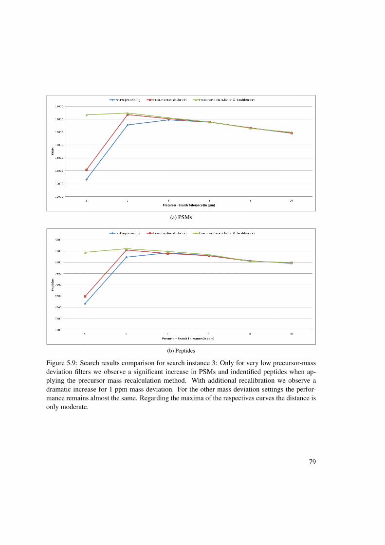
(a) PSMs
(b) Peptides
Figure 5.9: Search results comparison for search instance 3: Only for very low precursor-massdeviation filters we observe a significant increase in PSMs and indentified peptides when ap-plying the precursor mass recalculation method. With additional recalibration we observe adramatic increase for 1 ppm mass deviation. For the other mass deviation settings the perfor-mance remains almost the same. Regarding the maxima of the respectives curves the distance isonly moderate.
79

Method No Prep. PrecursorPrec. Imp.
PrecursorPrec. Imp. &Recalibration
Improvement
10 ppm Maximum Precursor Mass DeviationPSMs 16458 16425 16436 -0.13%Peptides 14933 14892 14900 -0.22%8 ppm Maximum Precursor Mass DeviationPSMs 16794 16758 16792 -0.01%Peptides 15133 15078 15109 -0.16%5 ppm Maximum Precursor Mass DeviationPSMs 17351 17521 17483 0.76%Peptides 15578 15697 15695 0.75%3 ppm Maximum Precursor Mass DeviationPSMs 16822 17717 17756 5.55%Peptides 15083 15851 15882 5.30%2 ppm Maximum Precursor Mass DeviationPSMs 15372 17460 17518 13.96%Peptides 13839 15675 15717 13.57%1 ppm Maximum Precursor Mass DeviationPSMs 11567 15142 15845 36.98%Peptides 10383 13579 14178 36.55%
Table 5.4: Results comparison for search instance 1: For each method, the highest PSMs- andidentified peptides values are written in bold. The last column gives the relative improvement ofthe precursor precision improvement & recalibration method in comparison to the unprocessedspectra.
The corresponding numbers are listed in table 5.7.
80

Method No Prep. PrecursorPrec. Imp.
PrecursorPrec. Imp. &Recalibration
Improvement
10 ppm Maximum Precursor Mass DeviationPSMs 7443 7497 7467 0.32%Peptides 4682 4738 4711 0.62%8 ppm Maximum Precursor Mass DeviationPSMs 7502 7528 7581 1.05%Peptides 4709 4730 4732 0.49%5 ppm Maximum Precursor Mass DeviationPSMs 7402 7580 7592 2.57%Peptides 4625 4733 4742 2.53%3 ppm Maximum Precursor Mass DeviationPSMs 6650 7300 7612 14.47%Peptides 4124 4510 4726 14.60%2 ppm Maximum Precursor Mass DeviationPSMs 5660 6845 7315 29.24%Peptides 3473 4179 4502 29.63%1 ppm Maximum Precursor Mass DeviationPSMs 3571 5336 5876 64.55%Peptides 2246 3239 3590 59.84%
Table 5.5: Results comparison for search instance 2: For each method, the highest PSMs- andidentified peptides values are written in bold. The last column gives the relative improvement ofthe precursor precision improvement & recalibration method in comparison to the unprocessedspectra.
81
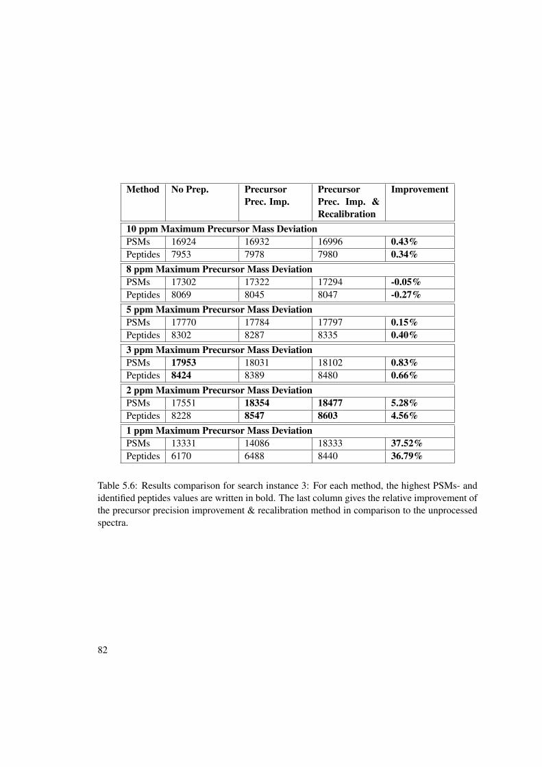
Method No Prep. PrecursorPrec. Imp.
PrecursorPrec. Imp. &Recalibration
Improvement
10 ppm Maximum Precursor Mass DeviationPSMs 16924 16932 16996 0.43%Peptides 7953 7978 7980 0.34%8 ppm Maximum Precursor Mass DeviationPSMs 17302 17322 17294 -0.05%Peptides 8069 8045 8047 -0.27%5 ppm Maximum Precursor Mass DeviationPSMs 17770 17784 17797 0.15%Peptides 8302 8287 8335 0.40%3 ppm Maximum Precursor Mass DeviationPSMs 17953 18031 18102 0.83%Peptides 8424 8389 8480 0.66%2 ppm Maximum Precursor Mass DeviationPSMs 17551 18354 18477 5.28%Peptides 8228 8547 8603 4.56%1 ppm Maximum Precursor Mass DeviationPSMs 13331 14086 18333 37.52%Peptides 6170 6488 8440 36.79%
Table 5.6: Results comparison for search instance 3: For each method, the highest PSMs- andidentified peptides values are written in bold. The last column gives the relative improvement ofthe precursor precision improvement & recalibration method in comparison to the unprocessedspectra.
82
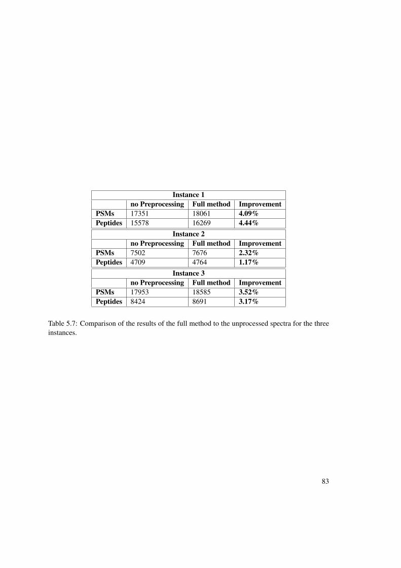
Instance 1no Preprocessing Full method Improvement
PSMs 17351 18061 4.09%Peptides 15578 16269 4.44%
Instance 2no Preprocessing Full method Improvement
PSMs 7502 7676 2.32%Peptides 4709 4764 1.17%
Instance 3no Preprocessing Full method Improvement
PSMs 17953 18585 3.52%Peptides 8424 8691 3.17%
Table 5.7: Comparison of the results of the full method to the unprocessed spectra for the threeinstances.
83


CHAPTER 6Conclusion and Future Work
In order to cope with the ever-increasing amount of data generated by high-throughput shotgun-proteomics experiments, methods that can order and divide the data have to be developed. Onepromising approach is the manipulation of recorded MS2-spectra as they contain the relevantdata that is sent to the database search engine and are the determining factor of the results ofa proteomics experiment. Moreover, the advances in accuracy and resolution of recent instru-ments allow the use of newer more accurate methods for spectrum manipulation which do applycomplex and less accurate techniques that were needed for spectra with lower resolutions.Therefore, in this thesis preprocessing methods for high resolution, high accuracy proteomicsdata with the aim of increasing the peptide identification performance of database search engineshave been discussed.
We analyzed existing deisotoping and deconvolution approaches for MS2-spectrum manip-ulation and experimented with possible improvements of the methods. The experiments wereconducted using three input instances consisting of a single .raw file and a set of three .raw files,respectively. In summary our experiments showed that only a moderate increase in PSMs can beachieved by these preprocessing steps. Furthermore, we made the interesting observation thatneither a refinement nor a degradation of the methods significantly changes this performance in-crease. This means that there is a balance in the scoring between the removal of as many peaksas possible and the selective removal of a few peaks. The conclusion that can be drawn fromthis first part of our work is therefore that spectrum cleaning can be useful to gain a few percentmore identified peptides. There is, however, not much more benefit to gain when using com-mon search engines such as Mascot, which do not take the mass precision of fragment ions intoaccount, that would justify the implementation of more sophisticated methods than the simplealready existing ones.
The second part of the work dealt with the development of an algorithm to improve the pre-cision of the precursor masses associated with the MS2-spectra that are sent to a search engine.We furthermore showed that the recalculation and recalibration methods significantly reducethe average, as well as the variance of ppm-errors in the identified peptides. This highly in-creases the results for searches with low precursor tolerance. However, the distance between
85

the best-performing tolerance using these methods and the best-performing tolerance withoutpreprocessing is not as significant. The reason is that common search engines, such as Mascotand SEQUEST, do not consider the distance of precursor ions to the matched peptide when thescore for the respective match is calculated.A new search engine that does take these distances into consideration is currently being devel-oped at the IMP Vienna in cooperation with the University of Applied Sciences Upper Austriaand is a starting-point for further experiments and developments of the proposed algorithm. Al-ternatively, a high-tolerance search followed by a rescoring and reranking of the obtained searchresults based on the mass tolerance is possible. In any case, it is necessary to account for theprecursor precision, since in our opinion it provides additional confidence in the matched pep-tide, even more, if the mass value is obtained as an average from several spectra following theelution profile of the respective peptide.
Besides the analysis of deisotoping and deconvolution and the development of a reliablemethod for the increase of precursor mass precision, several software products have resultedfrom this work. Most importantly, the algorithms were included in a plugin written in C# for theProteome Discoverer software, version 1.3.0.339, by Thermo Fisher Scientific, that can easilybe integrated into existing workflows.Additionally, the peak-reconstruction algorithm was implemented into two further softwareproducts:
• PeakAnalyzer: A module for SimpatiQCo, a quality control software for LC-MS/MS-systems.
• Spectrum Analyzer: A stand-alone tool for the analysis of .raw files.
Of course, in both cases, the MS2-spectrum manipulation, as well as the precursor mass preci-sion improvement, there is still room for further developments. Especially the peak-reconstruction,as well as the recalibration approach still offer room for improvement. E.g. the final evaluationof a reconstructred peak is lacking some kind of repair algorithm, in case a peak is probablynot originating from a single peptide. Here statistical approaches, such as the fitting of a bi-variate Gaussian could help in determining the part of the peak that should be kept. However,the integration of further enhancements would have gone beyond the scope of this thesis. It isnonetheless our ambition regarding future work to further improve and maintain the developedalgorithms.
86

List of Figures
2.1 Generic structure of an amino acid . . . . . . . . . . . . . . . . . . . . . . . . . . 62.2 Peptide bond formation . . . . . . . . . . . . . . . . . . . . . . . . . . . . . . . . 72.3 N- and C-termine of a peptide . . . . . . . . . . . . . . . . . . . . . . . . . . . . 72.4 Primary protein structure . . . . . . . . . . . . . . . . . . . . . . . . . . . . . . . 82.5 Structure levels of a protein . . . . . . . . . . . . . . . . . . . . . . . . . . . . . . 92.6 General composition of a mass spectrometer . . . . . . . . . . . . . . . . . . . . . 102.7 Scheme of a QExactive Orbitrap instrument . . . . . . . . . . . . . . . . . . . . . 112.8 Shotgun-proteomics workflow . . . . . . . . . . . . . . . . . . . . . . . . . . . . 132.9 Electrospray ionization process . . . . . . . . . . . . . . . . . . . . . . . . . . . . 152.10 The MS/MS-scan cycle . . . . . . . . . . . . . . . . . . . . . . . . . . . . . . . . 162.11 Possible Cleavage sites in a peptide . . . . . . . . . . . . . . . . . . . . . . . . . 182.12 Basic workflow of database search engines . . . . . . . . . . . . . . . . . . . . . . 202.13 Peptide sequence overlap between forward and reverse databases . . . . . . . . . . 232.14 The target-decoy search workflow . . . . . . . . . . . . . . . . . . . . . . . . . . 242.15 Excerpt of an MS1-spectrum schowing the m/z-values and intensities of some pro-
file points. . . . . . . . . . . . . . . . . . . . . . . . . . . . . . . . . . . . . . . . 27
3.1 Deisotoping of a simple isotope pattern . . . . . . . . . . . . . . . . . . . . . . . 323.2 Overlapping isotope patterns . . . . . . . . . . . . . . . . . . . . . . . . . . . . . 333.3 Probability distribution for the number of 13C-isotopes . . . . . . . . . . . . . . . 363.4 12C isotope ratio comparison . . . . . . . . . . . . . . . . . . . . . . . . . . . . . 373.5 1 13C isotope ratio comparison . . . . . . . . . . . . . . . . . . . . . . . . . . . . 383.6 2 13C isotope ratio comparison . . . . . . . . . . . . . . . . . . . . . . . . . . . . 383.7 3 13C isotope ratio comparison . . . . . . . . . . . . . . . . . . . . . . . . . . . . 393.8 Comparison of Mascot search results, example 1 . . . . . . . . . . . . . . . . . . 403.9 Comparison of Mascot search results, example 2 . . . . . . . . . . . . . . . . . . 403.10 Comparison of Mascot search results, example 3 . . . . . . . . . . . . . . . . . . 41
4.1 Constructing a 3d-peak from several 2d-peaks . . . . . . . . . . . . . . . . . . . . 494.2 Example of a 2d-split peak . . . . . . . . . . . . . . . . . . . . . . . . . . . . . . 504.3 Example of an ideal 3d-peak . . . . . . . . . . . . . . . . . . . . . . . . . . . . . 544.4 Example of a 3d-peak, in which a sudden m/z-shift occurs . . . . . . . . . . . . . 564.5 Example of 3d-peak, in which a continuous m/z-drift occurs . . . . . . . . . . . . 57
87

4.6 Example of 3d-peak split peak . . . . . . . . . . . . . . . . . . . . . . . . . . . . 584.7 Example of 3d-peak split peak that could not be detected . . . . . . . . . . . . . . 594.8 Extraction of several peaks per spectrum instead of one . . . . . . . . . . . . . . . 604.9 Recalibration of precursor m/z-values . . . . . . . . . . . . . . . . . . . . . . . . 624.10 A typical Proteome Discoverer workflow using both developed nodes . . . . . . . 64
5.1 MS2-spectrum Manipulation method comparison for instance 1. . . . . . . . . . . 695.2 MS2-spectrum Manipulation method comparison for instance 2 . . . . . . . . . . . 705.3 MS2-spectrum Manipulation method comparison for instance 3 . . . . . . . . . . . 715.4 ppm-error distribution comparison for search instance 1 . . . . . . . . . . . . . . . 735.5 ppm-error distribution comparison for search instance 2 . . . . . . . . . . . . . . . 745.6 ppm-error distribution comparison for search instance 3 . . . . . . . . . . . . . . . 755.7 Search results comparison for search instance 1 . . . . . . . . . . . . . . . . . . . 775.8 Search results comparison for search instance 2 . . . . . . . . . . . . . . . . . . . 785.9 Search results comparison for search instance 3 . . . . . . . . . . . . . . . . . . . 79
88

Bibliography
[1] Ruedi Aebersold and Matthias Mann. Mass spectrometry-based proteomics. Nature,422:198–207, 2003.
[2] Robert E. Ardrey. Liquid Chromatography - Mass Spectrometry: An Introduction. JohnWiley & Sons, Ltd, 2003.
[3] G. Audi and A.H. Wapstra. The 1995 update to the atomic mass evaluation. NuclearPhysics, A 595:409–480, 1995.
[4] Sean A Beausoleil, Judit Villén, Scott A Gerber, John Rush, and Steven P Gygi. Aprobability-based approach for high-throughput protein phosphorylation analysis and sitelocalization. Nature Biotechnology, 24:1285–1292, 2006.
[5] Jeremy M. Berg, John L. Tymoczko, and Lubert Stryer. Biochemistry, Sixth Edition. W.H.Freeman Company, New York, 2006.
[6] P. De Bievre and P.D.P. Taylor. IUPAC Recommended Isotopic Abundances. Int. J. MassSpectrom. Ion Phys., 123:149, 1993.
[7] Jürgen Cox and Matthias Mann. MaxQuant enables high peptide identification rates, indi-vidualized p.p.b.-range mass accuracies and proteome-wide protein quantification. NatureBiotechnology, 26:1367–1372, 2008.
[8] Jürgen Cox, Annette Michalski, and Matthias Mann. Software Lock Mass by Two-Dimensional Minimization of Peptide Mass Errors. J. Am. Soc. Mass Spectrom, 22:1373–1380, 2011.
[9] Robertson Craig and Ronald C. Beavis. A method for reducing the time required to matchprotein sequences with tandem mass spectra. Rapid Communications in Mass Spectrome-try, 17:2310–2316, 2003.
[10] Edmond de Hoffmann and Vincent Stroobant. Mass Spectrometry: Priciples and Applica-tions, Third Edition. John Wiley & Sons, Ltd, 2007.
[11] Peicheng Du and Ruth Hogue Angeletti. Automatic Deconvolution of Isotope-ResolvedMass Spectra Using Variable Selection and Quantized Peptide Mass Distribution. Analyti-cal Chemistry, 78, No. 10:3385–3392, 2006.
89

[12] Pehr Edman. Method for Determination of the Amino Acid Sequence in Peptides. ActaChemica Scandinavica, pages 283–293, 1950.
[13] Joshua E. Elias and Steven P. Gygi. Target-decoy search strategy for increased confidencein large-scale protein identifications by mass spectrometry. Nature Methods, 4, 3:207–214,2007.
[14] Joshua E. Elias and Steven P. Gygi. Target-Decoy Search Strategy for Mass Spectrometry-Based Proteomics. Methods Mol Biol., 604:55–71, 2010.
[15] Jimmy K. Eng, Ashley L. McCormack, and John R. Yates III. An Approach to CorrelateTandem Mass Spectral Data of Peptides with Amino Acid Sequences in a Protein Database.American Society for Mass Spectrometry, 5:976–989, 1994.
[16] John B. Fenn, Matthias Mann, Chin Kai Meng, Shek Fu Wong, and Craig M. Whitehouse.Electrospray Ionization for Mass Spectrometry of Large Biomolecules. Science, 246:64–71, 1988.
[17] Michael Guilhaus. Principles and Instrumentation in Time-of-flight Mass Spectrometry. J.Mass Spectrom., 30:1519–1532, 1995.
[18] Lukas Käll, Jesse D Canterbury, Jason Weston, William Stafford Noble, and Michael JMacCoss. Semi-supervised learning for peptide identification from shotgun proteomicsdatasets. Nature Methods, 4:923–925, 2007.
[19] Lukas Käll, John D. Storey, Michael J. MacCoss, and William Stafford Noble. AssigningSignificance to Peptides Identified by Tandem Mass Spectrometry Using Decoy Databases.Journal of Proteome Research, 7:29–34, 2008.
[20] Michael Karas and Franz Hillenkamp. Laser Desorption Ionization of Proteins with Molec-ular Masses Exceeding 10 000 Daltons. Analytical Chemistry, 60 (20):2299–2301, 1988.
[21] Paul J. Kersey, Jorge Duarte, Allyson Williams, Youla Karavidopoulou, Ewan Birney, andRolf Apweiler. The International Protein Index: An integrated database for proteomicsexperiments. Proteomics, 4:1985–1988, 2004.
[22] Thomas Köcher, Peter Pichler, Michael Schutzbier, Christoph Stingl, Axel Kaul, NilsTeucher, Gerd Hasenfuss, Josef M. Penninger, and Karl Mechtler. High precision quan-titative proteomics using iTRAQ on an LTQ Orbitrap: a new mass spectrometric methodcombining the benefits of all. Journal of Proteome Research, 8:4743–4752, 2009.
[23] Matthias Mann, Chin Kai Meng, and John B. Fenn. Interpreting Mass Spectra of MultiplyCharged Ions. Analytical Chemistry, 61:1702–1708, 1989.
[24] Melissa M. Matzke, Katrina M. Waters, Thomas O. Metz, Jon M. Jacobs, Amy C. Sims,Ralph S. Baric, Joel G. Pounds, and Bobbie-Jo M. Webb-Robertson. Improved qualitycontrol processing of peptide-centric LC-MS proteomics data. Bioinformatics, 27 no.20:2866–2872, 2011.
90

[25] Roger E. Moore, Mary K. Young, and Terry D. Lee. Qscore: An Algorithm for EvaluatingSEQUEST Database Search Results. J. Am. Soc. Mass Spectrom, 13:378–386, 2002.
[26] Nedim Mujezinovic. Improved Protein Identification after Fast Elimination of Non-Interpretable Peptide MS/MS Spectra and Noise Reduction. PhD thesis, Vienna Universityof Technology, 2007.
[27] Nedim Mujezinovic, Georg Schneider, Michael Wildpaner, Karl Mechtler, and FrankEisenhaber. Reducing the haystack to find the needle: improved protein identification afterfast elimination of non-interpretable peptide MS/MS spectra and noise reduction. BMCGenomics, I I, Supplement 1, 2010.
[28] Sven Nahnsen, Andreas Bertsch, Jörg Rahnenführer, Alfred Nordheim, and OliverKohlbacher. Probabilistic Consensus Scoring Improves Tandem Mass Spectrometry Pep-tide Identification. Journal of Proteome Research, 10:3332–3343, 2011.
[29] National High Magnetic Field Laboratory. http://www.magnet.fsu.edu/. Accessed: 2012-31-08.
[30] National Human Genome Research Institute. http://www.genome.gov. Accessed: 2012-06-20.
[31] Jesper V Olsen, Boris Macek, Oliver Lange, Alexander Makarov, Stevan Horning, andMatthias Mann. Higher-energy C-trap dissociation for peptide modification analysis. Na-ture Methods, 4, 9:709–712, 2007.
[32] Jesper V. Olsen, Shao-En Ong, and Matthias Mann. Trypsin cleaves exclusively C-terminalto Arginine and Lysine Residues. Molecular & Cellular Proteomics, 3.6:608–614, 2004.
[33] Akhilesh Pandey and Matthias Mann. Proteomics to study genes and genomes. Nature,405:837–846, 2000.
[34] DJC Pappin, D Rahman, HF Hansen, M Bartlet-Jones, W Jeffery, and AJ Bleasby. Chem-istry, mass spectrometry and peptide-mass databases: Evolution of methods for the rapididentification and mapping of cellular proteins. Mass Spectrometry in the Biological Sci-ences, pages 135–150, 1996.
[35] David N. Perkins, Darryl J. C. Pappin, David M. Creasy, and John S. Cottrell. Probability-based protein identification by searching sequence databases using mass spectrometry data.Electrophoresis, 20:3551–3567, 1999.
[36] Peter Pichler, Michael Mazanek, Frederico Dusberger, Lisa Weilnböck, Christian Huber,Christoph Stingl, Theo Luider, Werner L Straube, Thomas Köcher, and Karl Mechtler.SIMPATIQCO (SIMPle AuTomatIc Quality COntrol): A Server-Based Software Suitewhich Facilitates Monitoring the Time Course of LC-MS Performance Metrics on Orbi-trap Instruments. accepted: 17-09-2012.
91

[37] P. Roepstorff and J. Fohlman. Proposal for a Common Nomenclature for Sequence Ions inMass Spectra of Peptides. Biomedical Mass Spectrometry, 11, 11:601, 1984.
[38] Mikhail M Savitski, Toby Mathieson, Isabelle Becher, and Marcus Bantscheff. H-Score, aMass Accuracy Driven Rescoring Approach for Improved Peptide Identification in Modi-fication Rich Samples. Journal of Proteome Research, 9 (11):5511–5516, 2010.
[39] Michael W. Senko, Steven C. Beu, and Fred W. McLafferty. Determination of Monoiso-topic Masses and Ion Populations for Large Biomolecules from Resolved Isotopic Distri-butions. American Society for Mass Spectrometry, 6:229–233, 1995.
[40] Youting Sun, Jianqiu Zhang, Ulisses Braga-Neto, and Edward R Dougherty. BPDA - ABayesian peptide detection algorithm for mass spectrometry. BMC Bioinformatics, 11:490,2010.
[41] Danielle L. Swaney, Graeme C. McAlister, Matthew Wirtala, Jae C. Schwartz, John E.P.Syka, and Joshua J. Coon. A supplemental activation method for high efficiency elec-tron transfer dissociation of doubly protonated peptide precursors. Analytical Chemistry,79:477–485, 2007.
[42] Selene K. Swanson and Michael P. Washburn. The continuing evolution of Shotgun Pro-teomics. Drug Discovery Today: Targets, 10:719–725, 2005.
[43] John E. P. Syka, Joshua J. Coon, Melanie J. Schroeder, Jeffrey Shabanowitz, and Don-ald F. Hunt. Peptide and protein sequence analysis by electron transfer dissociation massspectrometry. Proc. Natl. Acad. Sci. U. S. A., 101, 26:9528–9533, 2004.
[44] Thomas Taus. phosphoRS: A novel probability-based algorithm for sensitive proteinphosphorylation-site localization from high-throughput LC-MS/MS data, Vienna Univer-sity of Technology, 2010.
[45] The Wikimedia Foundation. http://en.wikipedia.org. Accessed: 2012-31-08.
[46] Harry Towbin, Theophil Staehelin, and Julian Gordon. Electrophoretic transfer of proteinsfrom polyacrylamide gels to nitrocellulose sheets: procedure and some applications. ProcNatl Acad Sci USA, 76, No.9:4350–4354, 1979.
[47] Michael P. Washburn, Dirk Wolters, and John R. Yates III. Large-scale analysis of the yeastproteome by multidimensional protein identification technology. Nature Biotechnology,19:242–247, 2001.
[48] Valerie C. Wasinger, Stuart J. Cordwell, Anne Cerpa-Poljak, Jun X. Yan, Andrew A.Gooley, Marc R. Wilkins, Mark W. Duncan, Ray Harris, Keith L. Williams, and Dr. IanHumphery-Smith. Progress with gene-product mapping of the Mollicutes: Mycoplasmagenitalium. ELECTROPHORESIS, 16:1090–1094, 1995.
92

[49] Cathy H. Wu, Lai-Su L. Yeh, Hongzhan Huang, Leslie Arminski, Jorge Castro-Alvear,Yongxing Chen, Zhangzhi Hu, Panagiotis Kourtesis, Robert S. Ledley, Baris E. Suzek,C.R. Vinayaka, Jian Zhang, and Winona C. Barker. The Protein Information Resource.Nucleic Acids Research, 31, 1:345–347, 2003.
[50] Vicki H. Wysocki, George Tsaprailis, Lori L. Smith, and Linda A. Breci. Mobile andlocalized protons: a framework for understanding peptide dissociation. J. Mass Spectrom.,35:1399–1406, 2000.
[51] Ying Zhang, Zhihui Wen, Michael P. Washburn, and Laurence Florens. ImprovingProteomics Mass Accuracy by Dynamic Offline Lock Mass. Analytical Chemistry, 83(24):9344–9351, 2011.
[52] Roman A. Zubarev, Neil L. Kelleher, and Fred W. McLafferty. Electron Capture Disso-ciation of Multiply Charged Protein Cations. A Nonergodic Process. J. Am. Chem. Soc.,120:3265–3266, 1998.
93