improving hoist performance during the up-peak of tall ... · pdf fileimproving hoist...
TRANSCRIPT

Improving Hoist Performance during the Up-Peak of Tall Building Construction
by
Mohamed Kamleh
A thesis submitted in conformity with the requirements for the degree of Master of Applied Science
Civil Engineering University of Toronto
© Copyright by Mohamed Kamleh 2014

ii
Improving Hoist Performance during the Up-Peak of Tall Building
Construction
Mohamed Kamleh
Master of Applied Science
Civil Engineering
University of Toronto
2014
Abstract
Purpose: With the increased demand for tall buildings, it has become crucial to study current
construction methods with respect to this emerging construction environment. The increase in
height of buildings produces difficulties in the vertical delivery of resources. This study will
examine the hoist’s (a temporary construction elevator) performance and its impact on worker
delays.
Approach: First, a discrete event simulation model using Simphony.Net software was developed
to represent the morning delivery of workers. Data from site observations, manufacturers’ data,
and expert opinion were collected and incorporated. The model was verified and validated. Then
alternative strategies for hoist management were studied.
Findings: A combination of staggered arrivals and zoning for hoist operations have shown to
provide hoist performance improvements by reducing the waiting time of workers.
Value: This research tests new methods to decrease the waiting time of workers, and improve
the hoist’s performance.

iii
Acknowledgments
I would like to take this opportunity to graciously thank Professor Brenda McCabe for her
constant support, guidance and mentorship. I would like to acknowledge her dedication to this
project and my education, and her endless patience.
I would like to extent to thank my parents and siblings for their support and love. They have
helped me stay on track and provided me with the utmost support during times of frustration. I
would most certainly like to extent a special thanks to my sister, May, for her tremendous
support.
I would like to extend a special thanks to Nelly Pietropaolo and the entire student services staff
for making my experience remarkable, for their help and support throughout this endeavor.
Sincere appreciation goes to those who helped make this research as success: Dr. Simaan
AbouRizk at University of Alberta for allowing free use of his simulation modeling software,
Simphony.Net; Sam, Gokul, and Steve at Daniels Group for their enthusiastic support and time.
Finally, I would like to thank my friends for being there for me throughout my education. They
helped guide and motivate me and were there for me when I needed them.

iv
Table of Contents
Acknowledgments .......................................................................................................................... iii
Table of Contents ........................................................................................................................... iv
List of Tables ............................................................................................................................... viii
List of Figures ................................................................................................................................. x
List of Appendices ....................................................................................................................... xiii
Chapter 1 Introduction .................................................................................................................... 1
1.1 Background ......................................................................................................................... 1
1.2 Motivation ........................................................................................................................... 4
1.3 Research Objective ............................................................................................................. 5
1.4 Scope ................................................................................................................................... 5
1.5 Research Contributions ....................................................................................................... 6
1.6 Study Methodology ............................................................................................................. 6
1.7 Thesis Organization ............................................................................................................ 7
Chapter 2 Elevator and Hoist Planning ........................................................................................... 9
2.1 Elevator planning ................................................................................................................ 9
2.1.1 Elevators vs. Hoists ............................................................................................... 11
2.2 Hoist Operation during Up-Peak ...................................................................................... 12
2.2.1 Factors Affecting Hoist Performance ................................................................... 13
2.3 Hoist planning methods .................................................................................................... 15
2.3.1 Summary of Limitations of Current Methods ....................................................... 20
2.4 Summary of factors impacting hoist operation ................................................................. 21
Chapter 3 Analysis Method .......................................................................................................... 22
3.1 Numerical methods ........................................................................................................... 22
3.1.1 Linear Models ....................................................................................................... 22

v
3.1.2 Regression ............................................................................................................. 23
3.1.3 R-squared .............................................................................................................. 24
3.2 Simulation ......................................................................................................................... 25
3.2.1 Monte Carlo Simulation ........................................................................................ 25
3.2.2 Discrete Event Simulation .................................................................................... 26
3.3 Characteristics of Methods ............................................................................................... 26
3.4 Selected Method: Discrete-Event simulation .................................................................... 27
3.4.1 DES in Construction ............................................................................................. 28
3.4.2 Limitations of DES ............................................................................................... 29
3.4.3 DES Software in Construction .............................................................................. 29
3.4.4 Applicability of Method to Hoist Operation ......................................................... 29
Chapter 4 Development of the Proposed Model ........................................................................... 31
4.1 Introduction ....................................................................................................................... 31
4.2 Simphony.Net ................................................................................................................... 31
4.2.1 Main Interface ....................................................................................................... 32
4.2.2 Modelling Elements .............................................................................................. 33
4.2.3 Simphony’s modelling distributions ..................................................................... 36
4.3 Model Uses ....................................................................................................................... 38
4.3.1 Current operation of the hoist ............................................................................... 39
4.3.2 Alternative strategy for improving hoist performance .......................................... 40
4.3.3 Comparison of the arrival time functions ............................................................. 41
4.4 Model description ............................................................................................................. 41
4.4.1 User-Input component .......................................................................................... 44
4.4.2 Arrival of workers ................................................................................................. 46
4.4.3 Loading of the Hoist ............................................................................................. 49
4.4.4 Hoist operation ...................................................................................................... 52
vi
4.4.5 Output generation .................................................................................................. 61
4.5 Decisions during Model Development ............................................................................. 63
4.6 Model Factors ................................................................................................................... 65
4.6.1 Factors as user-inputs ............................................................................................ 66
4.6.2 Factors built into the model .................................................................................. 66
4.7 Model Output .................................................................................................................... 67
4.8 Model Scenarios ................................................................................................................ 68
4.9 Scenario components ........................................................................................................ 69
4.9.1 Model entities ........................................................................................................ 69
4.9.2 Model resources .................................................................................................... 69
4.9.3 The model programming ....................................................................................... 69
4.9.4 Model variables ..................................................................................................... 70
4.10 Model Verification and Validation ................................................................................... 71
4.10.1 Model verification ................................................................................................. 71
4.10.2 Validation .............................................................................................................. 72
4.11 Planning Options ............................................................................................................... 73
4.11.1 Site characteristics ................................................................................................ 73
4.11.2 Hoist characteristics .............................................................................................. 73
4.11.3 Stage of construction ............................................................................................. 73
4.11.4 Worker schedules .................................................................................................. 73
4.12 Chapter Summary ............................................................................................................. 73
Chapter 5 Impact of Model Inputs ................................................................................................ 75
5.1 Distribution of the arrival of workers ............................................................................... 75
5.2 Inter-arrival rates of workers ............................................................................................ 76
5.3 Impact of Hoist Characteristics ......................................................................................... 78
5.4 Impact of the number of workers and number of floors ................................................... 79

vii
Chapter 6 Using the Model to Improve Hoist Performance ......................................................... 84
Chapter 7 Conclusion and Recommendations .............................................................................. 91
7.1 Conclusions ....................................................................................................................... 91
7.2 Limitations of the study .................................................................................................... 92
7.3 Recommendations ............................................................................................................. 93
Bibliography ................................................................................................................................. 95
Appendices .................................................................................................................................. 101
viii
List of Tables
Table 1: Sample hoist speeds and capacities ................................................................................ 14
Table 2: Simple formulaic method for hoist planning .................................................................. 15
Table 3: Factors affecting hoist operation .................................................................................... 21
Table 4: Characteristics of Analysis Methods .............................................................................. 26
Table 5: Description of Simphony.Net modelling elements ......................................................... 33
Table 6: Example of alternative strategy schedule using step function ........................................ 40
Table 7: Difference between arrival of workers in the model scenarios ...................................... 41
Table 8: Example algorithm for input assignment ........................................................................ 45
Table 9: Example algorithm for assigning durations according to step function ......................... 47
Table 10: Sample algorithm for assigning hoist ID ...................................................................... 55
Table 11: Sample algorithm for directing the hoist ...................................................................... 55
Table 12: Sample algorithm for counting hoist cycles ................................................................. 56
Table 13: Sample algorithm for assigning travel durations .......................................................... 56
Table 14: Sample algorithm for tracking hoist travel ................................................................... 58
Table 15: Sample algorithm for checking if it is the final stop .................................................... 58
Table 16: Sample algorithm for checking if there is a stop .......................................................... 59
Table 17: Sample algorithm for resetting variables ...................................................................... 61
Table 18: Sample algorithm for trace data generation .................................................................. 62
Table 19: Input variables categories ............................................................................................. 65

ix
Table 20: Values of factors built into the model ........................................................................... 67
Table 21: Definition of model variables ....................................................................................... 70
Table 22: Validation through case studies .................................................................................... 72
Table 23: Summary of impact studies .......................................................................................... 75
Table 24: Summary of R-Squared values for different fits ........................................................... 81
Table 25: Inputs used in the analysis ............................................................................................ 84
Table 26: Arrival schedule details ................................................................................................ 85
Table 27: Cumulative delay for 50% and 80% of workers ........................................................... 90

x
List of Figures
Figure 1: Number of high-rise constructed per year in Toronto ..................................................... 3
Figure 2: Construction crane (left) and hoist (right) ....................................................................... 4
Figure 3: Decision variables (left) and planning method (Right) survey. .................................... 16
Figure 4: Simphony.Net’s main interface components ................................................................. 33
Figure 5: Uniform distribution ...................................................................................................... 37
Figure 6: Normal distribution ....................................................................................................... 37
Figure 7: Exponential distribution layout ..................................................................................... 38
Figure 8: Step function layout ....................................................................................................... 38
Figure 9: Flow chart of method used for modelling the hoist operation ...................................... 39
Figure 10: Hierarchy of the model ................................................................................................ 42
Figure 11: Sample scenario layout ................................................................................................ 43
Figure 12: Current operation scenario model inputs ..................................................................... 44
Figure 13: Procedure for defining model inputs ........................................................................... 45
Figure 14: Alternative strategy scenario model inputs ................................................................. 46
Figure 15: Model elements representing arrival of workers ......................................................... 49
Figure 16: Model elements representing loading of one hoist ...................................................... 50
Figure 17: Model elements representing loading of two hoists .................................................... 50
Figure 18: Model elements describing the loading of one hoist ................................................... 51
Figure 19: Model elements describing the loading of two hoists ................................................. 51

xi
Figure 20: Setting attributes for entities after hoist loading ......................................................... 52
Figure 21: Complete hoist cycle ................................................................................................... 53
Figure 22: Model elements describing initial launching of the hoist ............................................ 54
Figure 23: Release and capture of hoist ........................................................................................ 56
Figure 24: Branch elements directing hoist stops ......................................................................... 57
Figure 25: Return cycle of hoist .................................................................................................... 60
Figure 26: Allowing hoist loading ................................................................................................ 60
Figure 27: Capturing the output data ............................................................................................ 62
Figure 28: Elements allowing generation of graphical output ...................................................... 62
Figure 29: Example of graph Delay per Worker .......................................................................... 68
Figure 30: Example of graph Cumulative Distribution of Delay ................................................. 68
Figure 31: Examination of arrival distributions ............................................................................ 76
Figure 32: Study of the impact of the arrival rate on the average waiting time ........................... 77
Figure 33: Worker Delay graph using inter-arrival rates .............................................................. 78
Figure 34: Cumulative distribution showing effect of inter-arrival rates ..................................... 78
Figure 35: Examination of hoist speeds and capacity on the performance ................................... 79
Figure 36: Examination of the impact of the number of workers. ................................................ 80
Figure 37: Examination of the impact of the number of floors .................................................... 80
Figure 38: Study of linear fit as a model for number of floors ..................................................... 82
Figure 39: Study of quadratic fit as a model for number of floors ............................................... 83

xii
Figure 40: Study of power fit as a model for number of floors .................................................... 83
Figure 41: Results showing worker arrival cases using the delay graph. ..................................... 86
Figure 42: Results showing worker arrival cases using the cumulative distribution. ................... 87
Figure 43: Highlighting the impact of the Zoning on the hoist performance. .............................. 88
Figure 44: Highlighting the impact of the alternative strategy over one hour arrival time. ......... 89

xiii
List of Appendices
Appendix 1: References on Artificial Intelligence ..................................................................... 101
Appendix 2: Model programmed algorithms ............................................................................. 102

1
Chapter 1 Introduction
1
This chapter will present an overview of the thesis. Firstly, it will begin by providing a general
background of construction productivity. Secondly, the reader will be provided with the
objectives and scope of the study. Finally, the motivation and thesis organization will be
presented.
1.1 Background
The construction industry is one of the largest industries in North America. Construction in
Canada is a $171 billion industry, providing 1.24 million jobs (Zuppa 2014) and accounts for
about 7% of the country’s GDP (Statistics Canada 2014). It consumes 40% of the country’s
energy and 50 % of its primary resources (Zuppa 2014). Governments have traditionally sought
to invest in infrastructure construction to enhance the economy and provide jobs.
The construction industry is known for being highly competitive and risky. Contractors are
always seeking ways to reduce their costs and increase their chances of being the lowest bidder.
To remain competitive in construction, more has to be produced for each dollar spent (Dozzi and
AbouRizk 1993).
One of the most well-known and studied ways to reduce construction cost is improving
productivity. Construction productivity is a measure of how much output is produced for each
input of a resource, such as equipment, materials and labour. Project managers aim to improve
productivity by ensuring that the resources are allocated when and where they are needed. A
typical constraint to accomplishing a project as planned is the availability of resources
(Christodoulou et al. 2009).
Construction productivity can be expressed as production rate, unit person-hour rate, and
performance factor (Dozzi and AbouRizk 1993). Many factors impact productivity including
project scope, layout, weather and construction methods (Soekiman et al. 2011). Another factor
that impacts productivity is the time workers spend waiting for materials, equipment, or
instructions that are required for them to continue their work (Thomas 1991).
2
Over the past century, there has been a dramatic shift toward city living (Brown and Newbold
2012). To reduce urban sprawl, there has also been an increase in the number of high-rise
buildings, providing affordable living and efficient supply of services. There has been a steady
increase worldwide in the construction of high-rise buildings and this trend is projected to
continue (CTBUH 2011).
Several definitions have been used to distinguish the buildings in terms of height. The
nomenclature “tall building” may be used to describe a high-rise depending on: location,
proportion, and technologies used (CTBUH 2014). The location of a building provides the
context of how tall the building is in comparison to the surrounding structures. Proportion refers
to its height to width ratio. For example, a building with a height to width ratio of 10:1 is more
likely to be considered tall than a building with a height to width ratio of 1:1, even if the
buildings are of the same height. Finally, to be considered tall, the building must use the type of
technologies used in tall buildings, such as structural wind bracing or dampers. Supertall and
Megatall buildings are more specific in their definitions with minimum heights of 300 and 600
metres respectively.
Recently, the City of Toronto experienced a sharp increase in the construction of high-rise
buildings, as shown in Figure 1. The increase is expected to continue as the number of high-rises
under construction or proposed increases as demonstrated ( Figure 1). Furthermore, there has
been a shift towards high-rise residential buildings. In 2001, 96% of tall buildings were non-
residential (CTBUH 2012). In contrast, 88% of buildings being constructed in 2012 were
residential (CTBUH 2012). There are 15 buildings taller than 150 metres under construction in
Toronto, more than any other city in the western hemisphere (CTBUH 2012). Toronto is
projected to have 45 buildings taller than 150 metres by 2015, about a 3.5 times increase since
2005 (CTBUH 2012).

3
Figure 1: Number of high-rise constructed per year in Toronto (Skyscraper Center 2014)
This increase in high-rise construction in Toronto has introduced new challenges for project
managers. One of the issues project managers face as the buildings get higher is the efficient
vertical delivery of materials and labour, which are typically achieved using the tower crane and
hoist. A hoist is a temporary elevator that moves vertically along a mast structure that is erected
on the outside of a building. As the building progresses in height, the mast is extended.
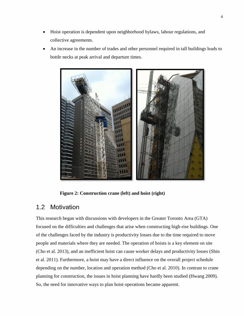
Figure 2 provides a picture of a crane and a hoist.
There are several reasons for the challenges in the vertical delivery of resources as the buildings
get higher.
The increase in the distance a hoist must travel with tall buildings poses a time challenge
in moving labour and material efficiently.
The increased wind speeds at greater heights and poor weather affecting visibility limit
the crane operations, thereby increasing the demand on the hoist for delivering materials.
Construction in Toronto usually means working in a limited space, which often also
limits the number of hoists that can be installed. Therefore, improving the productivity of
a single hoist is essential.
0
5
10
15
20
25
30
35
40
45
50
192
9
193
1
196
5
196
7
196
8
196
9
197
2
197
3
197
4
197
5
197
6
197
8
197
9
198
1
198
3
198
4
198
5
198
9
199
0
199
1
199
2
199
3
200
3
200
5
200
6
200
7
200
8
200
9
201
0
201
1
201
2
201
3
201
4
Pro
po
sed
Nu
mb
er o
f B
uil
din
gs
Co
mp
lete
d
Year
Toronto's High-rise Construction
4
Hoist operation is dependent upon neighborhood bylaws, labour regulations, and
collective agreements.
An increase in the number of trades and other personnel required in tall buildings leads to
bottle necks at peak arrival and departure times.
Figure 2: Construction crane (left) and hoist (right)
1.2 Motivation
This research began with discussions with developers in the Greater Toronto Area (GTA)
focused on the difficulties and challenges that arise when constructing high-rise buildings. One
of the challenges faced by the industry is productivity losses due to the time required to move
people and materials where they are needed. The operation of hoists is a key element on site
(Cho et al. 2013), and an inefficient hoist can cause worker delays and productivity losses (Shin
et al. 2011). Furthermore, a hoist may have a direct influence on the overall project schedule
depending on the number, location and operation method (Cho et al. 2010). In contrast to crane
planning for construction, the issues in hoist planning have hardly been studied (Hwang 2009).
So, the need for innovative ways to plan hoist operations became apparent.

5
1.3 Research Objective
The primary objective of this study is to improve hoist operations for high-rise building
construction, enabling an efficient delivery of workers during the morning peak.
A secondary objective is to compare operational strategies, such as staggered arrivals and
zoning, on the effectiveness of the hoist. Finally, the output will introduce a bench mark for
comparing alternative hoist management strategies in the future.
1.4 Scope
The scope of this study will be limited to high-rise residential building construction by
developers within the Greater Toronto Area (GTA). The focus on residential presents a worst-
case scenario in that office building interiors are often left unfinished when turned-over to the
user. Interior finishing is resource intensive and can have a major impact on the number of
construction hoists needed on a project.
The scope is also limited to the movement of labour during the morning peak. The morning peak
occurs when the workers arrive to site at the beginning of the shift, and are transported to
different floors in the building. This study will assume that during this morning peak only
workers will be transported in the hoist. This assumption has been validated using site
observations and expert opinion. The reasoning for this assumption is that most construction sites
use the hoist to solely deliver workers during the morning peak. Once the workers have been
delivered, the hoist will begin its mixed-used function of delivering both workers and materials.
This intense activity, of moving workers during the morning peak, is more complex than that of
materials because material delivery could be organized in advance and be scheduled during the
night or weekends (Park et al. 2013). Getting the workers to their work location faster during the
morning peak reduces delays and provides the hoist with more time for material delivery. Thus,
it has a direct influence on the overall project success.
Finally, although productivity is important, this research will focus on the efficiency and
effectiveness of hoists. Hoists are not in themselves a production unit but are instead service
equipment that allows all other work to be performed. Therefore, their productivity is not as
important as their ability to facilitate the real production units. So, throughout this thesis, hoist
efficiency and effectiveness will be used instead.

6
1.5 Research Contributions
This study provides the three contributions in the field of construction hoist operation
improvement:
A hoist model that reduces the number of user-inputs relative to previous models found in
the literature. As such, the model is more user-friendly.
An examination of the impact of changing the workers’ arrival to site on the hoist
efficiency has been conducted. This examination has not been previously conducted for
hoist operations.
Novel ways to present hoist effectiveness and efficiency for alternative management
strategies.
1.6 Study Methodology
The steps that were undertaken in this study were:
The problem was identified through discussions with experts in the field
A literature review was conducted and the limitations of previous efforts were identified
Factors affecting hoist operations were acknowledged
Data were collected to understand and formulate the operation of the hoist
DES was selected as the method of analysis to address the complex uncertainties in the
cyclic operation of a hoist.
Several iterations of the DES model were developed, verified and validated using data
from site and expert opinion. The iterations considered the impact of the factors and the
output
The final model is proposed and presented

7
The impact of the alternative approach, a combination of zoning and staggered arrivals of
workers, is demonstrated through an example.
1.7 Thesis Organization
This dissertation is organized according to the following sections:
Chapter 1-Introduction: This section provides an overview of the problem being studied.
First, an introduction to the need to study the productivity of construction methods in tall
buildings is presented. Second, the objective, scope and motivation of this research are
discussed. Finally, the approach and steps undertaken for this analysis are summarized.
Chapter 2-Hoists and Elevator Planning: A literature review of the research undertaken in
hoist and elevator planning is presented. This section defines the hoist operation
problem, the data collected, and the factors used for the analysis.
Chapter 3-Analysis Method: This section presents the selected analysis method for hoist
planning. In addition, it provides the reader with a description of the mathematical
models used for the analysis of the results. A description of discrete-event simulation and
regression is included.
Chapter 4-Development of the Proposed Model: This section describes the discrete-
event-simulation model. It will begin with the process undertaken in the development of
the model. Subsequently, it will outline the different components of the model and the
methods used for modeling the hoist operation.
Chapter 5-Impact of Model Inputs: An analysis of the model variables and output is
conducted. The study of the impact of each of the inputs of the model on the hoist
performance is included.
Chapter 6 –Using the Model to Improve Hoist Performance: An example of how the
method may be used for hoist planning is also presented through a hypothetical case
study of a tall building.

8
Chapter 7- Conclusion and Recommendations: This section concludes the dissertation.
Limitations and recommendations are presented for guiding future research of hoist
planning and performance improvements.

9
Chapter 2 Elevator and Hoist Planning
2
Due to the scarcity of previous work on hoist planning, a review of elevator planning studies was
undertaken to supplement this research. The similarities in the function of hoists and elevators
allow for a better understanding of how the study on hoist operation could be facilitated.
However, the differences between their operations prevent the use of elevator planning methods
for hoists. This chapter will begin by summarizing previous efforts in elevator planning. Then, it
will describe the similarities and differences between hoists and elevators. Finally, a review of
the research on the operation of construction hoists will be presented.
2.1 Elevator planning
Elevator planning methods range from numerical analysis to simulation techniques. These
methods aim to find an appropriate elevator configuration to serve the traffic during the
operating life of a high-rise building (Tervonena et al. 2008).
Elevator planning is dependent on the characteristic traffic profiles of different building types
(Benmakhlouf and Khator 1993). Office buildings typically have up-peak traffic at the start of
the work day, two-way or inter-floor traffic during the day, and down-peak traffic at the end of
the work day (Tervonena et al. 2008).
The up-peak is most commonly used for the design of elevator systems in office buildings
because it has the most demanding traffic. For this reason, analytical methods for calculating the
up-peak handling capacity and interval are most commonly used (Tervonena et al. 2008).
Early studies in elevator planning focused on developing formulas to estimate the average
waiting time and the round-trip time for elevator users, and these measures became the primary
indicators for elevator performance (Tervonena et al. 2008). The average waiting time (AWT) is
calculated by taking the mean of the actual time prospective passengers wait after registering a
hall call (or entering the waiting queue if a call has already been registered) until the responding
elevator doors begin to open (Cortés et al. 2004). The round-trip time (RTT) is defined as the
time between a passenger’s call for the elevator and when they reach the destination floor. The

10
calculation of round trip time is shown by Equation 1, and average wait time is shown by
Equation 2.
Equation 1: Round-trip time for elevators (Barney and Santos 1975)
𝑹𝑻𝑻 = 𝟐𝑯𝒕𝟏 + (𝑺 + 𝟏)𝒕𝟐 + 𝑷𝒕𝟑
𝑅𝑇𝑇 − 𝑅𝑜𝑢𝑛𝑑 𝑡𝑟𝑖𝑝 𝑡𝑖𝑚𝑒
𝐻 − 𝐻𝑖𝑔ℎ𝑒𝑠𝑡 𝑟𝑒𝑣𝑒𝑟𝑠𝑎𝑙 𝑓𝑙𝑜𝑜𝑟∗
𝑆 − 𝑒𝑥𝑝𝑒𝑐𝑡𝑒𝑑 𝑛𝑢𝑚𝑏𝑒𝑟 𝑜𝑓 𝑐𝑎𝑟 𝑠𝑡𝑜𝑝𝑠 𝑎𝑏𝑜𝑣𝑒 𝑡ℎ𝑒 𝑙𝑜𝑏𝑏𝑦∗
𝑃 − 𝑎𝑣𝑒𝑟𝑎𝑔𝑒 𝑐𝑎𝑟 𝑙𝑜𝑎𝑑
𝑡1 − 𝑖𝑛𝑡𝑒𝑟𝑓𝑙𝑜𝑜𝑟 𝑡𝑟𝑎𝑛𝑠𝑖𝑡 𝑡𝑖𝑚𝑒
𝑡2 − 𝑜𝑝𝑒𝑟𝑎𝑡𝑖𝑛𝑔 𝑡𝑖𝑚𝑒
𝑡3 − 𝑝𝑎𝑠𝑠𝑒𝑛𝑔𝑒𝑟 𝑡𝑟𝑎𝑛𝑠𝑓𝑒𝑟 𝑡𝑖𝑚𝑒
∗ −𝑻𝒉𝒆𝒔𝒆 𝒇𝒂𝒄𝒕𝒐𝒓𝒔 𝒄𝒐𝒖𝒍𝒅 𝒃𝒆 𝒂𝒕𝒕𝒂𝒊𝒏𝒆𝒅 𝒇𝒓𝒐𝒎 𝒂 𝒈𝒓𝒂𝒑𝒉
Equation 2: Average wait time for elevator (CIBSE 1993)
𝑨𝑾𝑻 = 𝟎. 𝟒𝑰𝑵𝑻 𝒇𝒐𝒓 𝒄𝒂𝒓 𝒍𝒐𝒂𝒅𝒔 𝒐𝒗𝒆𝒓 𝟓𝟎%
𝐼𝑁𝑇 − 𝐼𝑛𝑡𝑒𝑟𝑣𝑎𝑙 𝑎𝑟𝑟𝑖𝑣𝑎𝑙 𝑡𝑖𝑚𝑒 (𝑚𝑖𝑛𝑢𝑡𝑒𝑠)
The inter- arrival rate and the capacity of an elevator are factors that determine the performance
of an elevator. In an office building, it is suggested that the up-peak interval between arrivals of
passengers is 20-30s (Tervonena et al. 2008). Another suggestion is to use an up-peak arrival
pattern that follows a Poisson distribution with a mean of 23 persons/minute (Ladany and Hersh
1979). An alternative possibility is to use discrete arrivals of 10-15 persons every 5 minutes
(CIBSE 1993).
Once the arrival pattern is determined by the planners, it is used to calculate the average waiting
time for different elevator capacities and combinations. Depending on the acceptable average
waiting time decided by either the owner or designer, a suitable elevator design is selected.
With the increase in mixed-use buildings, the uncertainty in the behaviour of passengers
increases. Because the future behaviour of passengers is unknown, numeric approaches are not

11
always suitable. As such, simulation models become viable. But in practice, the simulation
methods have not progressed much from their initial development in the 1960s (Tervonena et al.
2008). Using simulation to study the morning peak period, it was concluded that: (i) it is
essential to determine the capacity of elevators and approximate a passenger’s waiting time
(Nagatani 2003), and, (ii) that the number of elevators is a major factor when accessing the up-
peak period (Nagatani 2004). Other important factors in determining an elevator’s performance
are the elevator’s speed, acceleration, door types, and the control algorithm (Tervonena et al.
2008).
One of the most commonly used simulation models in the elevator planning and design industry
is Elevate TM
(Peters 2014). This software simulates the performance of an elevator for different
types of buildings. However, through discussions with the developer, it was concluded that
elevator simulation models could not effectively be used for hoist planning. The differences in
the operation of the hoist and elevator limit the application of elevator simulation tools to its
intended purpose - elevators.
2.1.1 Elevators vs. Hoists
The operation of hoists and elevators is similar in concept; however, there are some differences
which render the elevator planning methods unsuitable for that of the hoist. Assumptions in
elevator planning software are (Cortés et al. 2004) :
Each call for the elevator is responded to by only one elevator, even if there are a lot of
people waiting.
The capacity of the elevator constitutes the maximum number of passengers transported.
The elevator stops at a floor only if there is a request to stop on that floor. Furthermore, an
elevator stops at a floor if there is a call, even if it is at capacity.
The elevator calls are consecutively arranged and met depending on the elevator trip
direction.
Elevators that are occupied cannot change the trip direction.

12
One of the major differences between elevators and hoists is in the operation of the system.
Elevators operate automatically within a fixed zone in accordance to a pre-set algorithm while
hoists are operated manually by an operator (Hwang 2009). Furthermore, the nature of
construction makes the hoist operation more dynamic than that of an elevator. The number of
stories, number of workers and working hours change as the construction progresses. With a
hoist, there is more flexibility in controlling the passenger traffic, by, perhaps, changing or
restricting the workers’ schedule. Although an elevator could not change direction if it is
occupied, this does not apply to a hoist. When a hoist is called, there is no pre-determined
destination programmed into the system.
Some similarities may be drawn between the operation of a hoist and an elevator in an office
building. The peaks for both situations occur at the beginning and the end of the work shift if the
transportation of people is considered only. Also, the arrival of workers is similar. It could be
assumed that the elevator and hoist are both bound by the capacity of the car. Furthermore, the
loading and unloading of workers is similar. When materials are not taken into consideration, the
hoist is unloaded similarly to that of an elevator in that both are dependent upon the opening and
closing times of the doors and the movement of workers in and out.
2.2 Hoist Operation during Up-Peak
Meetings with industry experts in the construction of tall buildings and hoist operators were
conducted to study the hoist operation. Construction site visits and recordings of hoist operations
were done to supplement the understanding of the problem at hand. During the meetings, the
project managers described the operation of the hoist and the factors that affect the hoist
operation. An investigation of hoist characteristics has been conducted using manufacturer’s
data.
The hoist operation is cyclic in nature. Typically, a hoist operation follows four steps during the
morning period:
1. Workers arrive to the construction site and wait for the next available hoist.
2. Workers board the hoist and relay their destination to the hoist operator.
3. The operator stops at the called floors and allows the workers to exit.

13
4. Hoist returns to the base of the building for further loading until all workers have been
delivered.
Note that this cycle only occurs in the delivery at the beginning of the work shift. After the
delivery of workers is complete, the hoist’s operation can be shifted to inter-floor transportation
and material delivery. This study will focus on the morning period. Once the method is tested,
the simulation could be expanded to other functions of the hoist.
2.2.1 Factors Affecting Hoist Performance
Worker Arrivals: The arrival of workers to a construction site can be similar to that of workers
to office buildings. However, depending on the scheduling of work by the project manager,
construction workers may take longer to arrive and their arrival can be more dispersed. For
example, some construction companies require their employees to gather at the start of their shift
and sign a safety form. Therefore, their arrival tends to be as one group; while others are
transported to the location as soon as they arrive to the site.
Number of Workers: The number of workers on site in a day is reliant on the project and
project stage. For example, typically at the final stage of the project the number of workers is
less than half that of the construction stage. However, the progress of the construction also plays
a role in the number of workers. If the project is behind schedule, more workers may be needed.
Hoist Departure Decisions: Another factor that affects the hoist operation is loading. As
workers arrive to site, they board the hoist. Typically, the hoist will transport all the workers that
are present even if it is not at capacity. Thus, the time the hoist waits for others to arrive directly
affects the total time of worker delivery.
Hoist Speed and Capacity: While hoist speeds provided by the manufacturers are accurate in
ideal situations, the operational speed is usually less, depending on the project, project stage,
number of stops and the experience of the operator. Table 1 provides examples of the hoist’s
speeds and capacity as provided by the manufacturers.
Hoist Cycle Time: The time it takes the hoist to complete a cycle is dependent on the number of
stops, building footprint, travel distance (number of stories and height of each storey) and speed
of the hoist. The number of workers is directly related to the footprint of the building.

14
Table 1: Sample hoist speeds and capacities
Hoist Type Single or
Double
Capacity
(persons)
Speed
(m/min) Source
Champion US-60-1R Single 27 45
(Metro Elevator 2013)
Champion US-60-2R
Twin Double 27 45
Champion US-6002-
1R Single 27 90
Champion US-6002-
2R Double 27 90
Champion US-80-1R Single 35 45 or
90
Champion US-80-2R Double 35 45 or
90
Hercules F 2200 SLS Both 27 15
(Bigge Crane and Rigging
Company 2014)
Hercules F 6000 SLS Both 30 40
Hercules F 7000 SHS Both 30 45
Hercules F 7000 SLS Both 25 100
PEGA 2832 TD VFC Both 25 100
PEGA 2840 TD VFC Both 20 100
Scando 650 Single 27 50
US-60-1Rx Single 27 45 or
90 (McDonough Elevators 2013)
US-60-2Rx Double 35 45 or
90
HS 80 Both 30 150
(USA Hoist 2014)
USA 7000 Both 27 100
Number of Hoists: In residential construction, the developer wants to minimize the number of
hoists because hoists delay the completion of the suites to which they are attached. This prevents

15
the developer from turning these suites over to the buyers, thereby reducing their cash flow.
Therefore, operating two hoists to their full potential, or adopting alternative strategies to
improve hoist performance is more desirable than adding additional hoists.
2.3 Hoist planning methods
One method for planning hoist operations uses empirical formulas based on experience from
construction projects (Cho et al. 2010). Table 2 shows an example of an existing hoist planning
method. This method is prone to error because it is dependent on the planner’s assumptions (Shin
et al. 2011). When this method is used for tall buildings, the experience is not sufficient to make
valid assumptions. Moreover, this method is used to estimate the required number of hoists;
however, it does not provide insight on how to improve a hoist’s productivity. Thus, the use of
the formulas has been minimal in industry.
Table 2: Simple formulaic method for hoist planning (Shin et al. 2011)
Phase description Formula Description
Transportation Frequency (Ft) Ft=a x b
a: Transportation frequency per
unit area based on historical
data of similar project(s)
b: Gross area of actual project
Transportation frequency per
day (Fd) Fd=Ft/n
n: Total construction duration,
days
Average height of
transportation(Ha) Ha=H x (1+C)
H: Height of Building
C: Charged rate for handicap
Cycle time of Transportation
(Tc) Tc=T1+T2+T3+T4
T1:Loading of hoist time
T2:Unloading of hoist time
T3:Time for lifting up
T4:Time for lifting down
Available Transportation
Frequency per day (Ta) Ta=(Tw/Tc)x d
Tw: Work time per day
D: Operation ratio of hoist
The adequate number of
temporary hoists(Nh) Nh=Fd/Ta
In 1996, a Scalable simulation model was used for elevator operations in construction of high-
rise buildings (Ioannou and Martinez 1996). The cyclic nature of the elevator operation is
modeled through a scalable code which allows the user to predetermine the number of stories.
This was the first attempt at modelling elevator operations in the context of construction.
However, the algorithm had been designed for an elevator as opposed to a hoist.

16
A survey was conducted with construction practitioners inquiring about their experience with
hoists, situations with inappropriate hoist planning, variables needed for hoist decision-making,
and methods used in projects for hoist planning (Hwang 2009). It was noted that almost 60% of
respondents reported cases and consequences of an inappropriate plan. Figure 3 demonstrates
some of the responses gathered in the survey. It is evident that the mathematical formulas are not
commonly used as a planning method for hoists. Also, the survey provided insight on the factors
that affect a hoist’s operation. Using the assembled data, the author proposed a discrete event
simulation model for the analysis of an effective plan for temporary hoists (Hwang 2009).
Simulation allows for the stochastic consideration of all the different factors inherent in hoist
operations. Furthermore, it may provide insight on ways to improve hoist performance.
Figure 3: Decision variables (left) and planning method (Right) survey (Hwang 2009).
A DES simulation model of a hoist operation was developed to calculate the hoist’s cycle time
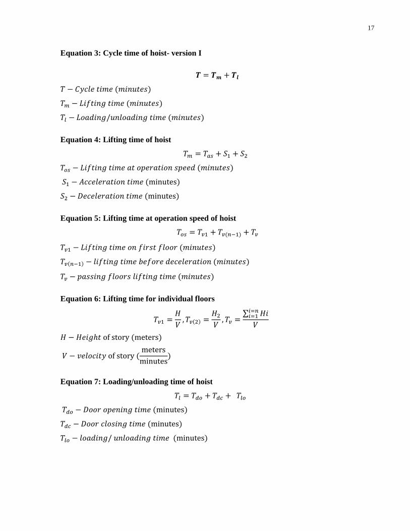
based on alternative demands (Cho et al. 2010). The hoist cycle time was then calculated using
Equations 4 to 7 and verified using the simulation and data collected from construction sites.
These equations are important for understanding the variables needed for simulating the
operation of the hoist. It is evident that the loading, unloading, acceleration and deceleration
times are required for the simulating the cycle time of the hoist.
17
Equation 3: Cycle time of hoist- version I
𝑻 = 𝑻𝒎 + 𝑻𝒍
𝑇 − 𝐶𝑦𝑐𝑙𝑒 𝑡𝑖𝑚𝑒 (𝑚𝑖𝑛𝑢𝑡𝑒𝑠)
𝑇𝑚 − 𝐿𝑖𝑓𝑡𝑖𝑛𝑔 𝑡𝑖𝑚𝑒 (𝑚𝑖𝑛𝑢𝑡𝑒𝑠)
𝑇𝑙 − 𝐿𝑜𝑎𝑑𝑖𝑛𝑔/𝑢𝑛𝑙𝑜𝑎𝑑𝑖𝑛𝑔 𝑡𝑖𝑚𝑒 (𝑚𝑖𝑛𝑢𝑡𝑒𝑠)
Equation 4: Lifting time of hoist
𝑇𝑚 = 𝑇𝑎𝑠 + 𝑆1 + 𝑆2
𝑇𝑜𝑠 − 𝐿𝑖𝑓𝑡𝑖𝑛𝑔 𝑡𝑖𝑚𝑒 𝑎𝑡 𝑜𝑝𝑒𝑟𝑎𝑡𝑖𝑜𝑛 𝑠𝑝𝑒𝑒𝑑 (𝑚𝑖𝑛𝑢𝑡𝑒𝑠)
𝑆1 − 𝐴𝑐𝑐𝑒𝑙𝑒𝑟𝑎𝑡𝑖𝑜𝑛 𝑡𝑖𝑚𝑒 (minutes)
𝑆2 − 𝐷𝑒𝑐𝑒𝑙𝑒𝑟𝑎𝑡𝑖𝑜𝑛 𝑡𝑖𝑚𝑒 (minutes)
Equation 5: Lifting time at operation speed of hoist
𝑇𝑜𝑠 = 𝑇𝑣1 + 𝑇𝑣(𝑛−1) + 𝑇𝑣
𝑇𝑣1 − 𝐿𝑖𝑓𝑡𝑖𝑛𝑔 𝑡𝑖𝑚𝑒 𝑜𝑛 𝑓𝑖𝑟𝑠𝑡 𝑓𝑙𝑜𝑜𝑟 (𝑚𝑖𝑛𝑢𝑡𝑒𝑠)
𝑇𝑣(𝑛−1) − 𝑙𝑖𝑓𝑡𝑖𝑛𝑔 𝑡𝑖𝑚𝑒 𝑏𝑒𝑓𝑜𝑟𝑒 𝑑𝑒𝑐𝑒𝑙𝑒𝑟𝑎𝑡𝑖𝑜𝑛 (𝑚𝑖𝑛𝑢𝑡𝑒𝑠)
𝑇𝑣 − 𝑝𝑎𝑠𝑠𝑖𝑛𝑔 𝑓𝑙𝑜𝑜𝑟𝑠 𝑙𝑖𝑓𝑡𝑖𝑛𝑔 𝑡𝑖𝑚𝑒 (𝑚𝑖𝑛𝑢𝑡𝑒𝑠)
Equation 6: Lifting time for individual floors
𝑇𝑣1 =𝐻
𝑉, 𝑇𝑣(2) =
𝐻2
𝑉, 𝑇𝑣 =
∑ 𝐻𝑖𝑖=𝑛𝑖=1
𝑉
𝐻 − 𝐻𝑒𝑖𝑔ℎ𝑡 of story (meters)
𝑉 − 𝑣𝑒𝑙𝑜𝑐𝑖𝑡𝑦 of story (meters
minutes)
Equation 7: Loading/unloading time of hoist
𝑇𝑙 = 𝑇𝑑𝑜 + 𝑇𝑑𝑐 + 𝑇𝑙𝑜
𝑇𝑑𝑜 − 𝐷𝑜𝑜𝑟 𝑜𝑝𝑒𝑛𝑖𝑛𝑔 𝑡𝑖𝑚𝑒 (minutes)
𝑇𝑑𝑐 − 𝐷𝑜𝑜𝑟 𝑐𝑙𝑜𝑠𝑖𝑛𝑔 𝑡𝑖𝑚𝑒 (minutes)
𝑇𝑙𝑜 − 𝑙𝑜𝑎𝑑𝑖𝑛𝑔/ 𝑢𝑛𝑙𝑜𝑎𝑑𝑖𝑛𝑔 𝑡𝑖𝑚𝑒 (minutes)

18
The inputs required of the simulation are (Cho et al. 2010) :
Total number of workers
Hoist capacity
Number of floors
Loading/unloading time
Door open and close time
Hoist speed
Number of hoists
A schedule of the workers and the destination floor.
While the simulation was verified to provide accurate cycle time calculations, several aspects
limit its use. First, providing a large amount of data has proven to be a difficult task in many
studies (Cho et al. 2010). A simulation model that eliminates the need for many input variables,
without jeopardizing the accuracy of the results, would be more user-friendly. Second, the output
of the cycle time of the hoist is not an effective indicator of its productivity. As the building gets
higher, the cycle time would naturally increase due to the travel time. However, the time lost
while workers are in a queue or waiting for a hoist is not reflected in this study.
A discrete-event simulation incorporating genetic algorithms was proposed to assist in optimal
hoist planning (Shin et al. 2011). The study focused on developing genetic algorithms for the
peak times of personnel and material hoisting. The proposed method addresses the long time
needed to use simple formulas or simulation in planning hoists (Shin et al. 2011). The formula
used for the cycle time of the hoist is represented in Equation 8. This equation demonstrates how
the operational efficiency and wait time are incorporated into the cycle time of the hoist, which
are factors that were not considered in equations 4-7.
Equation 8: Cycle time of the hoist- version II
𝑻𝒋(𝒋𝒕𝒉 𝒄𝒚𝒄𝒍𝒆 𝒕𝒊𝒎𝒆) = 𝒘𝒋 + 𝒍𝒋 + ∑ ((𝒇𝒌 − 𝒇𝒌−𝟏)𝒉
𝒔𝒆+ 𝒅𝒋𝒌)
𝒏
𝒌=𝟏
+ (𝑴𝑨𝑿(𝒇𝒌)𝒉
𝒔𝒆)
𝑤 − 𝑤𝑎𝑖𝑡𝑖𝑛𝑔 𝑡𝑖𝑚𝑒 (𝑚𝑖𝑛𝑢𝑡𝑒𝑠)

19
𝑙 − 𝑙𝑜𝑎𝑑𝑖𝑛𝑔 𝑡𝑖𝑚𝑒 (𝑚𝑖𝑛𝑢𝑡𝑒𝑠)
𝑓 − 𝑑𝑒𝑠𝑡𝑖𝑛𝑎𝑡𝑖𝑜𝑛 𝑓𝑙𝑜𝑜𝑟 𝑜𝑓 𝑒𝑎𝑐ℎ 𝑟𝑒𝑠𝑜𝑢𝑟𝑐𝑒 (𝑖𝑛𝑡𝑒𝑔𝑒𝑟)
ℎ − 𝑢𝑛𝑖𝑡 ℎ𝑒𝑖𝑔ℎ𝑡 𝑝𝑒𝑟 𝑠𝑡𝑜𝑟𝑦 (𝑚𝑒𝑡𝑒𝑟𝑠)
𝑠 − 𝑚𝑎𝑥𝑖𝑚𝑢𝑚 𝑠𝑝𝑒𝑒𝑑 (𝑚𝑒𝑡𝑒𝑟𝑠
𝑚𝑖𝑛𝑢𝑡𝑒)
𝑒 − 𝑜𝑝𝑒𝑟𝑎𝑡𝑖𝑜𝑛𝑎𝑙 𝑒𝑓𝑓𝑖𝑐𝑖𝑒𝑛𝑐𝑦 (%)
𝑑 − 𝑑𝑢𝑚𝑝𝑖𝑛𝑔 𝑡𝑖𝑚𝑒 (𝑚𝑖𝑛𝑢𝑡𝑒𝑠)
This model requires eleven inputs and provides the waiting time for the hoist and the queue
length as outputs (Shin et al. 2011). Although the outputs provided a better estimate of the hoist
performance in comparison to previous studies, it needed a larger number of inputs from the
user.
A combination of simulation and a Branch and Bound (B&B) algorithm was used to compare the
times to deliver workers by changing the delivery routes for the hoists (Cho et al. 2013). While
this tool is capable of providing the best hoist plan with respect to travel time, it falls short in
several areas. First, the destination of the workers is determined mathematically, which may be
inaccurate in real-life applications as worker destination is usually reliant on the type of work
and the construction schedule. Second, the operation of the hoist is optimized based on the total
time needed to deliver the workers. This is a direct function of the height of the building and
does not represent the time lost waiting for the hoist.
While hoist optimization has primarily focused on hoist selection, its operation is equally
important. The only operational practice suggested in the literature to improve hoist performance
was the concept of zoning. Zoning is an elevator operation strategy where cars are limited to
serving specific floors. A simulation model to evaluate the optimal zoning configuration for
hoists over the construction phase was developed (Park et al. 2013), but some challenges were
identified by the authors. First, the process of manually estimating the lifting-demand was time
consuming. Second, the zoning configuration of the hoists had to be adjusted as the construction
progressed. Updating the zoning too frequently may cause confusion to the workers while
updating less frequently may cause a mismatch between the lifting demand and frequency.
Further investigation is needed. While demand-based zoning could reduce the total hoist time by
approximately 40% (Park et al. 2013), the zones were optimized based on the total hoisting time

20
and the wait time by workers for the hoist was not considered. Therefore, the study does not
provide insight on productivity losses due to workers waiting for the hoist.
2.3.1 Summary of Limitations of Current Methods
While the previously developed methods for planning hoist operations have advanced this area,
their limitations make them difficult to use.
The numerical methods used to estimate the number of hoists required are rarely used in
industry. They are ineffective when the user does not provide the appropriate assumptions, and
they typically require a large number of input variables. Furthermore, they do not provide
suggestions to improve hoist effectiveness other than increasing the number of hoists, which as
already discussed, causes other challenges. Therefore, it is more effective to improve the
performance of the hoist.
None of the methods considered the arrival of the workers to the site as a factor. Elevator
productivity studies have shown that the arrival of passengers has a major impact on the
operation. Furthermore, most methods used the cycle time and the total time to deliver workers
as the output variable. However, this is not a complete indicator of the performance of hoists as it
does not indicate how much time is lost waiting for the hoist. The wait time, commonly used in
evaluating elevators, provides a better indication of how much time is lost.
While simulation was used to model the operation of a hoist, only one study presented an
operational management strategy to improve the efficiency of the operation.

21
2.4 Summary of factors impacting hoist operation
Using past research in both hoist operation and elevator planning, factors affecting the
performance of hoists have been compiled. These factors will be either input variables or
inherited within the model, depending on the factor type.
Table 3: Factors affecting hoist operation
Factor Source
(Hw
ang 2
009)
(Cho e
t al
. 2010)
(Shin
et
al. 2011)
(Par
k e
t al
. 2013)
(Lad
any a
nd H
ersh
1979
)
(Ter
vonen
a et
al.
2008
)
(CIB
SE
1993)
Number of Stories X X X
Number of Workers X X X
Arrival Distribution X X X
Mean arrival Rate X X X
Capacity of Hoist X X X X
Number of Hoists X X X X
Time per floor X X X
Loading/unloading Time X X X
Door open/Close Time X X X
Acceleration/Deceleration Time X X X
Speed of Hoist X X X
Number of stops X X X

22
Chapter 3 Analysis Method
3
This chapter will begin by providing a brief description of analysis methods. After an
introduction to and comparison of numerical methods and simulation, the chosen method of
analysis, discrete-event simulation (DES), is described in detail. It will also provide insight to
how DES has been used in the construction industry and why it is effective for studying hoist
operations.
Artificial intelligence (AI) methods, such as Bayesian belief networks and fuzzy logic, are
considered powerful tools for studying construction operations. After careful review, however, it
was decided that these tools will not be used in this research and therefore will not be discussed.
Appendix 1 provides a list of references that describe these methods for the reader’s interest.
3.1 Numerical methods
Numerical analyses solve problems in a numerical form (Gautschi 2012). These approaches are
used to solve problems with many variables and constraints and directly produce optimum points
(Arora 2012). Numerical models could be linear or non-linear, such as polynomials and
differential equations.
3.1.1 Linear Models
The simplest deterministic mathematical relationship between two variables is a linear form
(Devor 2009). The linear model is described in Equation 9.
Equation 9: Linear equation model
𝒚 = 𝜷𝟎 + 𝜷𝟏𝒙𝟏 + 𝜷𝟐𝒙𝟐 + 𝜷𝟑𝒙𝟑 … 𝜷𝒏𝒙𝒏
The x-variables are independent variables which influence the dependent variable y. One of the
methods for developing a linear model is regression. The following section provides an
introduction to regression.

23
3.1.2 Regression
Regression was introduced in 1869 by Sir Francis Galton in his book Hereditary Genius-An
enquiry into its laws and consequences (Bingham and Fry 2010). Regression has evolved since,
and many methods have been developed for the estimation of the equation’s parameters. Fitting
models by minimizing the sum of squares is the most commonly used method (Monahan 2001).
In a regression, it is assumed that the data points are collected independently and are randomly
distributed. Using the sum of squares, the vertical distance of the data points to the regression
line is minimized. The sum of squared vertical deviations from the points to a line is presented in
Equation 10.
Equation 10: Sum of squared vertical deviation (Devor 2009):
𝑓(𝑏0, 𝑏1) = ∑[𝑌 − (𝑏0
𝑛
𝑖=1
+ 𝑏1𝑥𝑖)]2
Using this, the coefficients of the variables are computed. The following equations are used to
calculate the slope and intercept of the linear equation.
Equation 11: Slope of linear equation
𝑏1 =∑(𝑥𝑖 − 𝜇𝑥)(𝑦𝑖 − 𝜇𝑦)
∑(𝑥𝑖 − 𝜇𝑥)2
𝑊ℎ𝑒𝑟𝑒 𝜇 𝑟𝑒𝑝𝑟𝑒𝑠𝑒𝑛𝑡𝑠 𝑡ℎ𝑒 𝑎𝑣𝑒𝑟𝑎𝑔𝑒 𝑜𝑓 𝑡ℎ𝑒 𝑣𝑎𝑟𝑖𝑎𝑏𝑙𝑒
Equation 12: Y-intercept of linear equation
𝑏0 =∑ 𝑦𝑖 − 𝑏1 ∑ 𝑥𝑖
𝑛
𝑊ℎ𝑒𝑟𝑒 𝑛 𝑖𝑠 𝑡ℎ𝑒 𝑛𝑢𝑚𝑏𝑒𝑟 𝑜𝑓 𝑑𝑎𝑡𝑎 𝑝𝑜𝑖𝑛𝑡𝑠
24
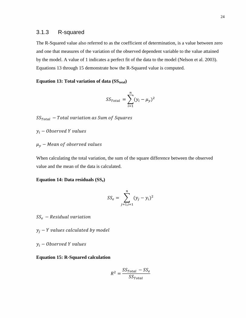
3.1.3 R-squared
The R-Squared value also referred to as the coefficient of determination, is a value between zero
and one that measures of the variation of the observed dependent variable to the value attained
by the model. A value of 1 indicates a perfect fit of the data to the model (Nelson et al. 2003).
Equations 13 through 15 demonstrate how the R-Squared value is computed.
Equation 13: Total variation of data (SStotal)
𝑆𝑆𝑇𝑜𝑡𝑎𝑙 = ∑(𝑦𝑖
𝑛
𝑖=1
− 𝜇𝑦)2
𝑆𝑆𝑇𝑜𝑡𝑎𝑙 − 𝑇𝑜𝑡𝑎𝑙 𝑣𝑎𝑟𝑖𝑎𝑡𝑖𝑜𝑛 𝑎𝑠 𝑆𝑢𝑚 𝑜𝑓 𝑆𝑞𝑢𝑎𝑟𝑒𝑠
𝑦𝑖 − 𝑂𝑏𝑠𝑒𝑟𝑣𝑒𝑑 𝑌 𝑣𝑎𝑙𝑢𝑒𝑠
𝜇𝑦 − 𝑀𝑒𝑎𝑛 𝑜𝑓 𝑜𝑏𝑠𝑒𝑟𝑣𝑒𝑑 𝑣𝑎𝑙𝑢𝑒𝑠
When calculating the total variation, the sum of the square difference between the observed
value and the mean of the data is calculated.
Equation 14: Data residuals (SSe)
𝑆𝑆𝑒 = ∑ (𝑦𝑗 − 𝑦𝑖
𝑛
𝑗=1,𝑖=1
)2
𝑆𝑆𝑒 − 𝑅𝑒𝑠𝑖𝑑𝑢𝑎𝑙 𝑣𝑎𝑟𝑖𝑎𝑡𝑖𝑜𝑛
𝑦𝑗 − 𝑌 𝑣𝑎𝑙𝑢𝑒𝑠 𝑐𝑎𝑙𝑐𝑢𝑙𝑎𝑡𝑒𝑑 𝑏𝑦 𝑚𝑜𝑑𝑒𝑙
𝑦𝑖 − 𝑂𝑏𝑠𝑒𝑟𝑣𝑒𝑑 𝑌 𝑣𝑎𝑙𝑢𝑒𝑠
Equation 15: R-Squared calculation
𝑅2 =𝑆𝑆𝑇𝑜𝑡𝑎𝑙 − 𝑆𝑆𝑒
𝑆𝑆𝑇𝑜𝑡𝑎𝑙

25
3.2 Simulation
Simulation provides a tool to study the behavior of systems that are too complex to study using
analytical methods (Halpin and Riggs 1992). Simulation models contain mathematical and
logical formulations that describe the behavior of systems over time (Naylor et al. 1996).
Simulation models may be characterized with respect to the method that they operate. The
classifications of simulation models can be described as (Rubinstein and Kroese 2007):
Static versus Dynamic Models: Static models are time invariant and tend to represent steady state
systems while dynamic models characterize systems that change with time increments.
Deterministic versus Stochastic Models: Deterministic models have pre-set relationships and
produce the same output given a set of initial conditions while stochastic models contain
randomness and therefore produce variable outputs even with the same initial conditions.
Continuous versus Discrete Models: In discrete models, the model is updated when events or
state variables change. These changes typically occur at uneven time intervals. Continuous
systems, on the other hand, are used to model continuous processes and are typically evaluated at
equal time steps.
3.2.1 Monte Carlo Simulation
Monte Carlo is a static and stochastic simulation which describes a variety of approaches that
conduct “what-if” analyses. It is a simulation method that relies upon the generation of random
numbers and statistical analysis to compute the results (Raychaudhuri 2008). The basic steps for
the Monte Carlo procedure are (Mooney 1997):
1. Develop a computer system to generate data by identifying a pseudo-population to generate
samples.
2. Sample from the population such that the data is representative of the statistical situation
being studied.
3. Calculate a desired characteristic in the sample and collect the information in a vector.
4. Redo Steps 2 and 3 for a predetermined number of trials.
5. Develop a frequency distribution of the results from the trials. This is estimate of
the sampling distribution of the characteristic under the circumstances specified.

26
3.2.2 Discrete Event Simulation
Discrete-event simulation (DES) models possess a state of data that captures the salient variables
of the system at any point in time (Altiok and Melamed 2007). In very general terms, the
methodology of DES systems is the following (Halpin and Riggs 1992):
1. Fix the simulation time to an initial value.
2. Create events, their connections and set their duration.
3. If the event list is empty, the simulation run is terminated. Otherwise, find the awaiting event
and unlink it from the event list.
4. Progress the simulation time to that of the most impending event, and execute it
5. Redo steps 2 and 3 until the simulation is terminated.
3.3 Characteristics of Methods
The use of the appropriate analysis method to represent a problem is important. Table 4
summarizes when a method is used and the advantages and limitations of each method.
Table 4: Characteristics of Analysis Methods
Type Method Use Advantages Disadvantages
Numerical
methods
Regression Used to represent the
effect of independent
variables on a
dependent variable
Provide insight on
the effect of each
variable on the
output
Very flexible
Model easily used
and modified
Underlying
assumptions must be
validated
Not effective in
modelling stochastic
variables
Simulation Monte Carlo Uses random number
generation to study
different alternatives
and impacts
Probabilistic
results of the
outcome
Allows for
multiple scenario
analysis
Effectively model
stochastic systems
Results depend on the
number of runs
Time-consuming to
develop and conduct
Difficult to validate
Not very user friendly
Discrete
Event
Uses events with
discrete durations to
represent a process
In many instances, a hybrid of more than one method was used to model a solution for a
problem. Hybrid methods usually complement each other’s weaknesses, thus producing a better
and more effective model.

27
3.4 Selected Method: Discrete-Event simulation
This section will introduce in more detail discrete-event simulation and why it is suitable for
modelling hoist operations.
A discrete-event simulation model is a representation of a system. The key elements in a DES
model are variables and events. There are three variable types in a DES model (Ross 2013):
1. Time variables: amount of simulated time that has elapsed.
2. Counter variables: keep track of the number of times an event has occurred.
3. System state variables: describe the state of the system at a certain time.
Discrete-event simulation is a representation of discrete events through which entities flow.
Whenever entities pass through an event, the values of the model variables change (Ross 2013).
The major aspects of DES systems are described next.
Model: A model is the representation of the operation being studied. A model is limited by
its boundaries and assumptions. A simulation model is typically created using nodes that
represent an action or activity. Nodes are connected by arrows that represent the flow of
entities (e.g. people, equipment or materials) from node to node.
Event: An event is a time-constrained occurrence that changes the system. An event in the
model, also referred to as a task, is a time or occurrence that delays the entities for a period of
time. For example, the time it takes a truck to travel could be represented in the model as the
“travel” event with the associated time. The duration of an event could be fixed, drawn from
a distribution, or depend upon other model variable states.
Entities: Entities represent an object that moves in the model and may represent workers,
equipment, materials, or any other entity in the system.
Attributes: Attributes are variables assigned to describe entity characteristics.
Resources: A resource is an object that provides a service to entities with a pre-determined
function. A resource is captured and used. For example, a resource could be an excavator that
loads trucks when they arrive at a loading event. The resource can be limited to a specific

28
quantity, so if a resource is not available, the entities wait for one to become available before
continuing into the event.
3.4.1 DES in Construction
Construction sites are unique in nature and therefore require a production plan catered to its
individual characteristics. Therefore, construction planning methods must be flexible to
accommodate the variable environment (Cho et al. 2011). The cyclic nature of construction
activities and the ability to easily evaluate construction alternatives are also challenging for
traditional methods (Chen and Huang 2013); (Levitt et al. 1999).
DES provides an alternative to traditional methods and has therefore been widely used to
represent the variable cyclic operations in construction. Built-in flexibility in DES allows for the
study of unique characteristics of a construction site and can easily represent the cyclic nature in
construction operations (Martinez J. C. 2010).
A very useful technique for the quantitative examination of operations and processes that occur
during the life cycle of a constructed project (Martinez J. C. 2010), simulation can be used to
examine and compare the performance of different construction approaches (Ioannou and
Martinez 1996). The steps for building a DES model in the construction engineering and
management field are (Martinez J. C. 2010):
1. Determine if DES is the appropriate method of analysis by understanding how the model can
be used to understand the system and evaluate performance.
2. Understand what questions need to be answered by the model and limit the scope and the
boundary accordingly.
3. Define how detailed the model will be and the features of the operation are. This is attained
by defining the elements, logic and model components will be used.
4. Collect data of the operation being modelled. The data should describe the probabilistic
assumptions and distribution fits that will be fed into the model.
5. Verify the model by ensuring the results and function is as expected. Validate the model
using data from the system.
6. Assess the output of the model for a single run.
7. Design simulation experiments and test the output to determine the performance of different
options.

29
8. Document the results and use them for determining the favorable options.
3.4.2 Limitations of DES
The assumption in DES is that the time between events is negligible; however, real world
activities are continuous; nothing is innately discrete (Puri and Martinez 2013). Therefore, a
modeller must ensure that the discretization assumptions are valid in the situation being studied.
Also, activity durations must represent the “real-world” scenario. Discretization, transforming
continuous processes into discrete-events, provides a significant improvement in the
computational performance during simulation (Puri and Martinez 2013).
DES is used to make decisions prior to implementation of the proposed changes in the field.
Therefore, it is not possible to completely validate the model by comparing it to real-world
output (Martinez J. C. 2010), but it is possible to model existing operations for validation
purposes.
3.4.3 DES Software in Construction
The use of DES in construction is credited to the development of CYCLONE by Haplin in 1977
(Hajjar and AbouRizk 2002). CYCLONE is a general-purpose modelling interface which allows
the user to use embodied functions to model a scenario. Since the development of CYCLONE,
many construction simulation interfaces have been developed such as INSIGHT (Paulson 1978),
RESQUE (Chang 1987), UM-CYCLONE (Ioannou P. 1989), CIPROS (Tommelein and Odeh
1994), STROBOSCOPE (Martinez J. C. 1996).
3.4.4 Applicability of Method to Hoist Operation
Typically, the problems that are well suited to DES include (Martinez J. C. 2010), (Ruwanpura
and Ariaratnam 2007):
1. Situations with significant uncertainties in the time required for an event and/or resource
quantities, operation and organization.
2. Situations that are logistically complicated with numerous dynamic rules and decisions that
change according to the context of the situation. Simulation provides an alternative to study
the behaviour of these complex systems. It offers a method of direct and detailed
observations. Using Simulation allows for the development of an approximate solution.

30
3. Problems that have interdependent components subject to variable event start-up conditions
that includes many resources that must collaborate in a complex organization.
4. Simulation provides an alternative to modelling problems which are difficult to model with
other mathematical methods.
5. If it is difficult to conduct a physical experiment, simulation provides an alternative to
conducting studies and observing the results.
Hoist operation is dependent upon many factors, and thus uncertainties lie in its tasks. The
arrival of workers, hoist breakdowns, stage of construction, and changes in schedule are
examples of the types of factors that produce uncertainty in a hoist’s operation. The operations of
a hoist and the decisions for locating and scheduling are complex in nature. The inter-linked
dependence of the hoist and construction schedule makes it very difficult to optimize the
operation of a hoist alone without considering its impacts on other activities. Furthermore, when
tall buildings are being studied, the complexity increases. As such, these characteristics of a hoist
operation are well suited for DES modeling.

31
Chapter 4 Development of the Proposed Model
4
The purpose of this chapter is to present the process used to develop the simulation model of the
hoist operation, along with a description of the model itself. First, the simulation modeling
environment software is introduced to the reader. Second, the iterations and factors of the model
are outlined. Finally, the model components and strategy are described.
4.1 Introduction
To ensure that the model meets the objectives of the study, several elements have been
considered. First, flexible designs enable managers to respond easily and cost-effectively to
changing circumstances (de Neufville and Scholtes 2011). To enable the representation of
different projects, project stages and characteristics, the model should allow the user to easily
change the inputs of the model. The model should also enable future expansion to other peak
times and to include the delivery of material.
Second, the model outputs should provide useful feedback on the different strategies under study
and allow direct comparisons between strategies. Moreover, the output must reflect not only the
operations of the hoist but of the labour delays caused by the hoist as well.
Third, the model must be developed for easy use. Thus, it must limit the number of inputs needed
while not compromising the modelling accuracy. Previous models required many user inputs,
which made their use time-consuming and less attractive to industry users. As such, this model
will automate as many inputs as possible.
Finally, using the model to study alternative operational strategies for hoists is important. This
will enable the planner to test ways to improve the hoist operations.
4.2 Simphony.Net
Simphony.Net (AbouRizk S. 2014) is a well-established DES software in both the research
community and the construction industry. Developed at University of Alberta, it has been

32
graciously provided for this research. Along with its user-friendly environment, it provides
support for (AbouRizk 2014):
Working in a user-friendly integrated interface environment
Modeling complicated scenarios by enabling modular and hierarchical structures
Storing and recovering frequently used simulation model layouts
Creating and using special purpose templates such as earthmoving, along with traditional
simulation templates such as CYCLONE
Writing user code to compute functions beyond the standard elements
Customizing the output with tools such as charts and tables
Producing automated data outputs in a standard form
4.2.1 Main Interface
The main interface of Simphony.Net is comprised of several components (Figure 4) as briefly
described next. For a more detailed description, the reader is directed to the Simphony.Net’s user
guide (AbouRizk S. 2014).
Modelling Space is the workspace for developing the graphical simulation model. Independent
modelling spaces can be created for each model scenario.
Template area contains the standard modelling elements.
Ribbon bar contains the file, view, run and help menus.
Model explorer window allows the user to view the files that comprise the structure of the model
and select scenarios and composite elements.
Property window lists the properties of model components, including scenarios and elements.
Properties are modifiable by the user and include probabilistic distributions to define activity
durations, model controls, or physical attributes,

33
Trace window provides the user with the text specified using a trace element or the errors
attained during modelling.
Figure 4: Simphony.Net’s main interface components
4.2.2 Modelling Elements
To supplement the reader’s understanding of Simphony.Net, a summary of selected modelling
elements is included in Table 5. This summary has been developed using the template manual
provided by the software’s developers. For a more detailed description of the elements, the
reader is directed to the general template manual (AbouRizk S. 2014).
Table 5: Description of Simphony.Net modelling elements
Element Symbol Description
Comment
Allows the user to add comments as text in the model.
Modelling Space
Ribbon Bar
Template
Area
Model
Explorer
Property
Grid
Trace Window

34
Element Symbol Description
Create
Creates entities at different quantities that leave the
element at user specified time distributions.
Task
Used to represent an activity. An entity is delayed for a
specific period of time. The task completion is also
dependent upon the availability of a server.
Counter
Increments a user-specified quantity each time an entity
passes through the element.
Set Attribute
Allows the user to assign attributes to the passing
entities.
Destroy
Deletes any entities that arrive at the element.
Execute
Allows the user to customize an action using user-
written code every time an entity passes through the
element.
Composite
A child group of elements that are grouped within a
scenario.
Trace
Allows the user to track the progress of the model by
outputting user-specified text.
Branch
Directs the entity to a different path based on either a
user –specified probability or condition.

35
Element Symbol Description
Generate
Used to clone a quantity of entities from an original
entity.
Consolidate
Merges a quantity of entities.
Batch
Merges a quantity of entities that could be unmerged
using an Unbatch element.
Unbatch
Unmerges a group of batched entities.
Resource
Identifies a resource in the model.
File
Tracks the waiting of entities for resources.
Capture
Allows the entities to capture resources.
Release
Allows the entities to release resources.
Preempt
Captures a resource with priority over a capture
element.
Statistic
Used to compute statistics on parameters in the model.

36
Element Symbol Description
StatisticCollect
Adds observations to a statistic element.
Valve
Stop or allow the entities to pass.
Chart
Displays data in a user-specified chat format.
ChartCollect
Receives an entity and collects the data points.
4.2.3 Simphony’s modelling distributions
Symphony.net has built in statistical distributions that allow for probabilistic modelling. The
following describes the distributions that have been used in the model.
The Constant distribution is a deterministic user-defined value.
The Uniform distribution describes a scenario when all values between a and b have an equal
probability of occurrence, as shown in Figure 5. The uniform distribution is commonly used for
random number generation.

37
Figure 5: Uniform distribution
The Normal distribution is one of the most commonly used distributions in modelling. It
describes many observed phenomena such as heights and weights. As a symmetric distribution,
the average has the highest probability of occurring. Figure 6 demonstrates the shape of the
normal distribution.
Figure 6: Normal distribution
The Exponential distribution (Figure 7) is shaped such that the probability increases faster as x
increases. For example, it can describe the arrivals of workers to office buildings in the morning.
The distribution is demonstrated.
Uniform Distribution
a b
P(x)
Pro
bab
ility
X-values
Normal Distribution

38
Figure 7: Exponential distribution layout
The Step function (Figure 8) describes occurrences where a group of x values share the same
probability. For example, the first 5 individuals that buy a product have an equal probability of
getting a certain price, and the probability that the price increases changes with each 5 buyers.
Figure 10 provides an example of how the step function could be displayed. Note that the step
function is not built in Simphony.Net’s modelling elements. However, this function has been
utilized by programming it into the model.
Figure 8: Step function layout
4.3 Model Uses
This section will describe the two components to modelling hoist operations: (i) modelling the
current operation of the hoist, and (ii) providing an alternative method for improving the
operation of the hoist.
Pro
bab
ility
X-values
Exponential Distribution
Pro
bab
ility
X-Values
Step Function

39
4.3.1 Current operation of the hoist
In this component of the model, the operation of the hoist is based on descriptions found in the
literature, through site observation, and from expert knowledge. Two scenarios are studied,
representing a single or double hoist. Figure 9 provides the flow chart of the method. Each of the
colors in this figure represents a component in the model which will be described in Section 4.4
Figure 9: Flow chart of method used for modelling the hoist operation

40
4.3.2 Alternative strategy for improving hoist performance
Two operational strategies have been included in the model to allow the user to improve the hoist
effectiveness by 1) staggering arrivals in which the workers arrive at different times, and, 2)
using zoning concepts to schedule the destination floors.
Zoning is a concept widely used in elevators and refers to predetermining the destination floors.
Many office and residential tall buildings have elevators that only travel to specific floors to
reduce elevator waiting times. While elevators are designed to only travel to specific floors,
hoists could be managed in a similar way. In this strategy, workers arrive at different times
depending on their destination floors or “zones”.
The staggered arrivals concept has been studied in transportation and elevator planning in office
buildings. Staggering arrivals reduces the queue that occurs. While this concept theoretically
achieves lower waiting times for elevators, it is usually difficult to implement due to the lack of
control of the arrivals. However, because the project manager is responsible for all personnel on
site, it is possible to schedule different trades to start work at different times. The distribution of
arrivals in these scenarios is the step function as shown in Table 6.
As an example, the first group of workers could be scheduled to arrive at 7:00 am and are
transported to floors 60-70 (zone 1), while the following group of workers are scheduled to
arrive at 7:15 am and are transported to floors 40-59.
Table 6: Example of alternative strategy schedule using step function
Group Number of Workers Time between Group Arrivals (mins) Destination floors
1 40 15
60-70
2 60 40-59
15
3 50 1-39
The impact of using this planning strategy on the hoist will be demonstrated through an example
in Chapter 6.

41
4.3.3 Comparison of the arrival time functions
The distribution used in the arrival time for the current operation and alternative strategy is the
main difference between the scenarios. Table 7 highlights the difference in the arrival of workers
and assignment of floors for workers.
Table 7: Difference between arrival of workers in the model scenarios
Operation Arrival Distribution Destination
Current Operation Constant inter-arrival time between
workers
Randomly assigned to any floor in
building
Alternative
Strategy
Step function between group of
workers
Zone assigned by user for each
group
4.4 Model description
This section will describe the model, which has four scenarios in a hierarchy structure as shown
in Figure 10. Within each scenario, the composite modelling element has been used to group a
sub collection of elements that come together for a specific purpose.
To describe the model for the reader, it has been divided into four main sections: (i) variable
input, (ii) arrival of workers and loading of hoist, (iii) operation of hoist, and, (iv) generation of
output. All these components work in tandem to provide a functional model. Figure 11 shows the
overall model. Each of these model components will be described including the components for
the current hoist operation and the alternative strategy.

42
Level 1: Model Level 2: Scenario Level 3: Composite
Pro
po
sed
Mod
el
S1: Single Hoist Current Operation
Arrival of workers
Wait for Hoist
Global Variables
S2: Single Hoist Alterative Strategy
Arrival of workers
Wait for Hoist
Global Variables
S3: Double Hoist Current Operation
Arrival of workers
Wait for Hoist
Global Variables
Hoist Selection
S4: Double Hoist Alterative Strategy
Arrival of workers
Wait for Hoist
Global Variables
Hoist Selection
Figure 10: Hierarchy of the model

43
Figure 11: Sample scenario layout
1-V
ari
ab
le I
np
ut
4-G
ener
atio
n o
f O
utp
ut
3-O
per
ati
on
of
Hois
t
2-A
rriv
al
of
work
ers
an
d l
oad
ing o
f h
ois
t
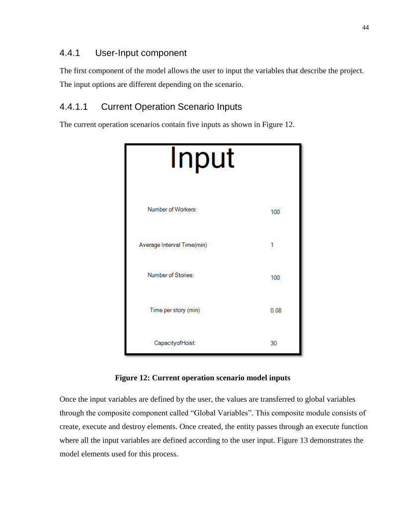
44
4.4.1 User-Input component
The first component of the model allows the user to input the variables that describe the project.
The input options are different depending on the scenario.
4.4.1.1 Current Operation Scenario Inputs
The current operation scenarios contain five inputs as shown in Figure 12.
Figure 12: Current operation scenario model inputs
Once the input variables are defined by the user, the values are transferred to global variables
through the composite component called “Global Variables”. This composite module consists of
create, execute and destroy elements. Once created, the entity passes through an execute function
where all the input variables are defined according to the user input. Figure 13 demonstrates the
model elements used for this process.

45
Figure 13: Procedure for defining model inputs
The execute elements runs the following algorithm (Table 8) to equate the variables in the model
to the values inputted by the user.
Table 8: Example algorithm for input assignment
Element: Execute Name: Assign array and
random variables
Scenarios:
1 hoist, current operation
2 hoists, current operation
Public Partial Class Formulas
Public Shared Function Formula(ByVal context As
Simphony.General.Execute) As System.Boolean
Redim context.Scenario.Ints(600)
Dim a as Comment = context.Scenario.GetElement(of Comment)("1")
Dim c as Comment = context.Scenario.GetElement(of Comment)("3")
Dim e as Comment = context.Scenario.GetElement(of Comment)("5")
Dim f as Comment = context.Scenario.GetElement(of Comment)("6")
dim g as Comment = context.Scenario.GetElement(of comment)("7")
context.Scenario.ints(203)=Cint(a.Text)
Context.Scenario.floats(2)=(cdbl(c.text))
context.Scenario.Ints(213)=Cint(e.Text)
Context.Scenario.floats(1)=cdbl(f.Text)
Context.Scenario.Ints(205) = Cint(g.Text)
Return true
End Function
End Class
4.4.1.2 Alterative strategy scenarios inputs
The alternative strategy scenarios allow the user to select the number of workers for different
groups, with the time between the groups and the destination for these groups. An example from
the model is displayed in Figure 14. The elements used in the model are same as the ones
presented in Figure 13 for the current operation scenarios.

46
Figure 14: Alternative strategy scenario model inputs
4.4.2 Arrival of workers
Once the global variables are assigned, the arrival of workers begin according to the distribution
and rate assigned by the user input. A composite function contains the elements used to model
the arrival of workers.
First, a large number of entities are created at Time=0 representing the workers. To model the
inter-arrival rate, the entities pass through a task, whose duration is dependent on the scenario
being used. For the current operation scenarios, the interval of the task is a constant distribution
with the value provided by the user. An inter-arrival duration of zero represents the workers
arriving all at the same time whereas and value greater than zero separates their arrivals. In the
alternative strategy scenarios, the task’s duration is based on the schedule inputted by the user.
This has been programmed as shown in Table 9. A “Pseudo” resource, not representing an actual
resource, is used to ensure that one entity passes the task at a time.
Once the entities arrive, they are randomly assigned a floor between 0 and the number of stories
completed. Also, the time of arrival of each worker is recorded as an attribute of the entity. This
will allow tracking of the assigned destination and time of arrival of each worker individually.

47
Finally, the number of workers is maintained according to the user input. This is done through a
branch element which ensures only the required number of workers pass through to load the
hoist.
Figure 15 provides a sample of the elements used in the model.
Table 9: Example algorithm for assigning durations according to step function
Element: Execute Name: Assign array and
random variables
Scenarios:
1 hoist, Alterative strategy
2 hoists, current operation
Public Partial Class Formulas
Public Shared Function Formula(ByVal context As
Simphony.Modeling.Task(Of Simphony.Simulation.GeneralEntity)) As
System.Double
Dim N1 as Comment = context.Scenario.GetElement(of Comment)("N1")
Dim N2 as Comment = context.Scenario.GetElement(of Comment)("N2")
Dim N3 as Comment = context.Scenario.GetElement(of Comment)("N3")
Dim N4 as Comment = context.Scenario.GetElement(of Comment)("N4")
dim N5 as Comment = context.Scenario.GetElement(of comment)("N5")
Dim T1 as Comment = context.Scenario.GetElement(of Comment)("T1")
Dim T2 as Comment = context.Scenario.GetElement(of Comment)("T2")
Dim T3 as Comment = context.Scenario.GetElement(of Comment)("T3")
Dim T4 as Comment = context.Scenario.GetElement(of Comment)("T4")
Dim L1 as Comment = context.Scenario.GetElement(of Comment)("L1")
Dim L2 as Comment = context.Scenario.GetElement(of Comment)("L2")
Dim L3 as Comment = context.Scenario.GetElement(of Comment)("L3")
Dim L4 as Comment = context.Scenario.GetElement(of Comment)("L4")
dim L5 as Comment = context.Scenario.GetElement(of comment)("L5")
Dim H1 as Comment = context.Scenario.GetElement(of Comment)("H1")
Dim H2 as Comment = context.Scenario.GetElement(of Comment)("H2")
Dim H3 as Comment = context.Scenario.GetElement(of Comment)("H3")
Dim H4 as Comment = context.Scenario.GetElement(of Comment)("H4")
dim H5 as Comment = context.Scenario.GetElement(of comment)("H5")
Dim W as Counter = context.Scenario.GetElement(of
Counter)("workers")
Select Case W.Count
'1
Case is <= Cint(N1.text)
Context.CurrentEntity.Ints(0)=
Cint(uniform.sample((Cint(L1.text)),(Cint(H1.text))))
Return 0
Case (Cint(N1.text)+1)
Context.CurrentEntity.ints(0)=
Cint(uniform.sample((Cint(L2.text)),(Cint(H2.text))))
Return Cdbl(T1.text)

48
'2
Case is <= (Cint(N2.text)+Cint(N1.text))
Context.CurrentEntity.Ints(0)=
Cint(uniform.sample((Cint(L2.text)),(Cint(H2.text))))
Return 0
Case (Cint(N2.text)+Cint(N1.text)+1)
Context.CurrentEntity.ints(0)=
Cint(uniform.sample((Cint(L3.text)),(Cint(H3.text))))
Return Cdbl(T2.text)
'3
Case is <= (Cint(N3.text)+Cint(N2.text)+Cint(N1.text))
Context.CurrentEntity.Ints(0)=
Cint(uniform.sample((Cint(L3.text)),(Cint(H3.text))))
Return 0
Case Cint(Cint(N3.text)+Cint(N2.text)+Cint(N1.text)+1)
Context.CurrentEntity.ints(0)=
Cint(uniform.sample((Cint(L4.text)),(Cint(H4.text))))
Return Cdbl(T3.text)
'4
Case is <=
(Cint(N4.text)+Cint(N3.text)+Cint(N2.text)+Cint(N1.text))
Context.CurrentEntity.Ints(0)=
Cint(uniform.sample((Cint(L4.text)),(Cint(H4.text))))
Return 0
Case (Cint(N4.text)+Cint(N3.text)+Cint(N2.text)+Cint(N1.text)+1)
Context.CurrentEntity.ints(0)=
Cint(uniform.sample((Cint(L5.text)),(Cint(H5.text))))
Return Cdbl(T4.text)
'5
Case is <=
(Cint(N5.text)+Cint(N4.text)+Cint(N3.text)+Cint(N2.text)+Cint(N1.text))
Context.CurrentEntity.Ints(0)=
Cint(uniform.sample((Cint(L5.text)),(Cint(H5.text))))
Return 0
End select
Return nothing
End Function
End Class

49
Figure 15: Model elements representing arrival of workers
4.4.3 Loading of the Hoist
Once the workers arrive for scenarios with two hoists, an algorithm embedded in nested branch
elements determine which hoist is available for loading. The algorithm asks the following
questions and directs the workers accordingly:
Is Hoist 1 available?
o If yes, is Hoist 2 also available?
If both hoists are available allow worker to load any hoist.
If only hoist one is available, load hoist one.
If no, is hoist two available?
If yes, load hoist two.
If no, wait for a hoist to be available.

50
Figure 16 and Figure 17 demonstrate a sample from the model for the selection of either one or
two hoists depending on the scenario.
Figure 16: Model elements representing loading of one hoist
Figure 17: Model elements representing loading of two hoists
The first entity to enter a hoist is passed into a task that has a duration of one minute. The hoist is
launched through a valve element in two cases, if the hoist has been loaded up to capacity or the

51
first entity has completed the one minute task. This will ensure that the hoist does not wait for
more than one minute.
If no hoist is available, the entities are redirected to a composite element called “wait for hoist”.
In this element the entities, wait for a hoist to become available.
This is presented in Figure 18 and Figure 19 from the model.
Figure 18: Model elements describing the loading of one hoist
Figure 19: Model elements describing the loading of two hoists
After a hoist is launched, data on the workers that have loaded the hoist is collected. The number
of stops on each floor and the final stop for that trip is assigned to global variables.
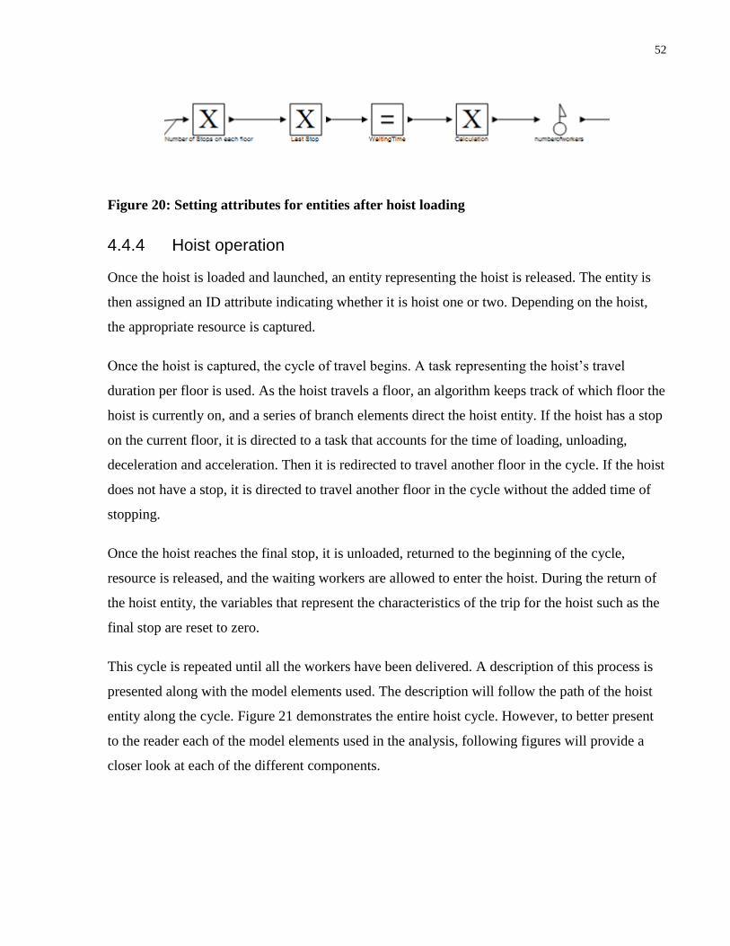
52
Figure 20: Setting attributes for entities after hoist loading
4.4.4 Hoist operation
Once the hoist is loaded and launched, an entity representing the hoist is released. The entity is
then assigned an ID attribute indicating whether it is hoist one or two. Depending on the hoist,
the appropriate resource is captured.
Once the hoist is captured, the cycle of travel begins. A task representing the hoist’s travel
duration per floor is used. As the hoist travels a floor, an algorithm keeps track of which floor the
hoist is currently on, and a series of branch elements direct the hoist entity. If the hoist has a stop
on the current floor, it is directed to a task that accounts for the time of loading, unloading,
deceleration and acceleration. Then it is redirected to travel another floor in the cycle. If the hoist
does not have a stop, it is directed to travel another floor in the cycle without the added time of
stopping.
Once the hoist reaches the final stop, it is unloaded, returned to the beginning of the cycle,
resource is released, and the waiting workers are allowed to enter the hoist. During the return of
the hoist entity, the variables that represent the characteristics of the trip for the hoist such as the
final stop are reset to zero.
This cycle is repeated until all the workers have been delivered. A description of this process is
presented along with the model elements used. The description will follow the path of the hoist
entity along the cycle. Figure 21 demonstrates the entire hoist cycle. However, to better present
to the reader each of the model elements used in the analysis, following figures will provide a
closer look at each of the different components.

53
Figure 21: Complete hoist cycle

54
A create element is used to produce two entities, each representing a hoist. The entities pass
through an execute function which sets an attribute for each entity to identify it as either hoist
one or two. A branch is then used to direct each entity to its path. Once the entities are directed,
they wait at a valve element which is opened by having the hoist at either capacity or if it has
been waiting more than one minute, which occurs in the loading of the hoist cycle. The
algorithms used in the execute and branch elements are displayed in Tables Table 10 and Table
11, respectively.
Figure 22: Model elements describing initial launching of the hoist

55
Table 10: Sample algorithm for assigning hoist ID
Element: Execute Name: Assign Hoist
Number
Scenarios:
All
Public Partial Class Formulas
Public Shared Function Formula(ByVal context As
Simphony.General.Execute) As System.Boolean
context.scenario.ints(211)= context.scenario.ints(211)+ 1
Context.currententity.Ints(2)= context.scenario.ints(211)
Return true
End Function
End Class
Table 11: Sample algorithm for directing the hoist
Element: Branch Name: Hoist 1 or 2 Scenarios:
All
Public Partial Class Formulas
Public Shared Function Formula(ByVal context As
Simphony.General.Branch) As System.Boolean
If context.CurrentEntity.Ints(2) = 1 then
Return true
end if
Return False
End Function
End Class
After either valve is opened, the entity captures the associated hoist resource. An execute
function is then used to count the number of cycles that is taken by each hoist. The entity is then
passed through a task which has a duration that represents travelling a single floor by the hoist.
This task takes the time per story inputted by the user and reduces the amount provided by 80%.
This aligns with the observations from site and expert opinion. This is demonstrated in Figure
23, Table 12 and Table 13.

56
Figure 23: Release and capture of hoist
Table 12: Sample algorithm for counting hoist cycles
Element: Execute Name: Number of Trips
for H1
Scenarios:
All
Public Partial Class Formulas
Public Shared Function Formula(ByVal context As
Simphony.General.Execute) As System.Boolean
Context.Scenario.Ints(207)=context.Scenario.Ints(207)+1
Return true
End Function
End Class
Table 13: Sample algorithm for assigning travel durations
Element: Task Name: Travel 1 Floor Scenarios:
All
Public Partial Class Formulas
Public Shared Function Formula(ByVal context As
Simphony.Modeling.Task(Of Simphony.Simulation.GeneralEntity)) As
System.Double
Return (Context.Scenario.floats(1)*0.8)
End Function
End Class

57
Once an Entity has traveled a floor, an execute element tracks the floor the hoist is on. Then a
group of branch elements are used to direct the hoist based on the value of the counter according
to the following logic:
Is there a stop on this floor?
o If yes: Is it the final stop?
If yes, go to the return cycle
If no, pass through a task which takes accounts for the acceleration,
deceleration, loading and unloading time components and then return to
travel another floor.
o If no, then go back to traveling another floor
Figure 24 demonstrates the model elements used for this process. Table 14, Table 15 and Table
16 will also demonstrate the algorithms used in these elements to model this operation.
Figure 24: Branch elements directing hoist stops

58
Table 14: Sample algorithm for tracking hoist travel
Element: Execute Name: Floor Counter Scenarios:
All
Public Partial Class Formulas
Public Shared Function Formula(ByVal context As
Simphony.General.Execute) As System.Boolean
Dim H as Integer
H = context.CurrentEntity.Ints(2)
Select case H
Case 1
context.Scenario.Ints(202) = context.Scenario.Ints(202)+1
Case 2
context.Scenario.Ints(302) = context.Scenario.Ints(302)+1
End Select
Return true
End Function
End Class
Table 15: Sample algorithm for checking if it is the final stop
Element: Branch Name: More Floors to go? Scenarios:
All
Public Partial Class Formulas
Public Shared Function Formula(ByVal context As
Simphony.General.Branch) As System.Boolean
Dim H as Integer
H = context.CurrentEntity.Ints(2)
Select case H
Case 1
If context.Scenario.Ints(201) = Context.Scenario.Ints(202) then
Return false
End if
Case 2
if context.Scenario.Ints(301) = context.Scenario.Ints(302) then
Return False
End If
End Select
Return true
End Function
End Class

59
Table 16: Sample algorithm for checking if there is a stop
Element: Task Name: Stop on Current
Floor?
Scenarios:
All
Public Partial Class Formulas
Public Shared Function Formula(ByVal context As
Simphony.General.Branch) As System.Boolean
Dim H as Integer
H = context.CurrentEntity.Ints(2)
Select case H
Case 1
If context.Scenario.Ints(Context.Scenario.Ints(202))> 0
then 'there is a stop
context.Scenario.Ints(Context.Scenario.Ints(202))=0
return true
End if
Case 2
If context.Scenario.Ints(400+Context.Scenario.Ints(302))> 0
then 'there is a stop
context.Scenario.Ints(400+Context.Scenario.Ints(302))=0
return true
End if
End Select
'There is no stop
Return false
End Function
End Class
Finally, once the entity has completed all the stops of the hoist, it is sent through the return cycle.
In this cycle, a task is used to represent the return trip of the hoist. Furthermore, the hoist
resource is released, and the variables are reset to zero. This will allow the hoist to be reloaded.
Thus, a valve controlling the loading of the hoist is opened by passing the entity through an
activator element. And the release of the hoist is restricted by another activator, this will ensure
that the hoist is only launched by the loading of the hoist operation, which is based on capacity
or waiting time. Figure 25 and Figure 26, present the modelling elements used for the return
cycle. Table 17 demonstrates the algorithm used for resetting the variables.

60
Figure 25: Return cycle of hoist
Figure 26: Allowing hoist loading

61
Table 17: Sample algorithm for resetting variables
Element: Execute Name: Reset variables Scenarios:
All
Public Partial Class Formulas
Public Shared Function Formula(ByVal context As
Simphony.General.Execute) As System.Boolean
Dim H as Integer
H = context.CurrentEntity.Ints(2)
Select case H
Case 1
Context.Scenario.Ints(200)=0
Context.Scenario.Ints(201)=0
Context.Scenario.Ints(202)=0
For A as Integer = 0 to 150
Context.Scenario.Ints(A) = 0
Next
context.Scenario.Ints(215) = 0
Case 2
Context.Scenario.Ints(301)=0
context.Scenario.Ints(300)=0
Context.Scenario.Ints(302)=0
context.Scenario.Ints(216)=0
End Select
Return true
End Function
End Class
4.4.5 Output generation
As the final worker is being loaded into the hoist, the outputs are computed. The waiting time of
each worker is stored as an attribute to the entity. Chartcollect and statisticscollect elements are
used to track the delay of each worker and the statistics of that delay. These elements provide the
user with a graph of the delay of each worker in order of arrival along with the histogram and
cumulative delay of the waiting times. The user could display these graphs for a single run or all
runs by selecting the statistics and chart elements shown in Figure 27.
Finally, a branch checks whether it is the final worker. Once the final entity passes, the average
waiting time is outputted to the user in a trace element. The algorithm used for the output is
shown in Table 18.

62
Figure 27: Capturing the output data
Figure 28: Elements allowing generation of graphical output
Table 18: Sample algorithm for trace data generation
Element: Execute Name: Data Scenarios:
All
Public Partial Class Formulas
Public Shared Function Formula(ByVal context As Simphony.General.Trace)
As System.String
Dim numofhoist as Integer
Select case context.Scenario.Name
Case "1 Hoist-CS"
numofhoist = 1
Case " 2 Hoist-CS"
numofhoist= 2
End select
Return " |Senario| "& context.Scenario.name & " |numofhoists| "
&Cstr(numofhoist) &" |no. of workers-Actual| "&
Cstr(Context.Scenario.Ints(203))& " |Average Arrival interval| "&

63
Cstr(context.scenario.floats(2))&" |no. of stories| "&
Cstr(Context.Scenario.Ints(213))&" |timeperfloor| "&
Cstr(context.Scenario.floats(1))&" |Capacity| "&
Cstr(context.Scenario.Ints(205))&" |Avg Wating time| "&
Cstr(context.Scenario.floats(6))&" |Max Wating time| "&
Cstr(context.Scenario.floats(3))
End Function
End Class
4.5 Decisions during Model Development
This section summarizes the modeling decisions and iterations that have been undertaken with
details provided in later sections.
1. Determination of Inputs: When the model was first developed, all the factors affecting the
hoist (see Table 3) were user-defined inputs. However, to reduce the number of user-defined
inputs, the impact of each input on the model output was studied, resulting in the number of
user-defined inputs being reduced from 12 to five. This was achieved by embedding the other
variables in the model and using typical values. The results have been compared to those
from other studies and similar results were obtained. Section 4.6 outlines the specific factors
and the impact analysis of the input variables is presented in Chapter 5.
2. Determination of output/decision variables: Several output statistics were tested for their
ability to adequately describe hoist productivity. These include:
The hoist’s cycle time
Total time for the delivery of workers
Percentage of workers waiting a certain time
Average waiting time of workers
It was decided that the hoist’s cycle time and total time for the delivery were not meaningful
indicators of productivity because they are both dependent on the height of the building.
Further, the time lost by workers waiting for the hoist is not reflected in these factors. The
percentage of workers waiting greater than 5, 10 and 15 minutes was also considered. While

64
this factor provides how many workers wait in the queue, the total time lost waiting for the
hoist is not reflected.
The average waiting time has been widely used in the planning of elevators, but not for the
planning of hoists. While the average waiting time provides an overall picture of the
operation, it is limited in the ability to provide feedback on the times that the hoist
effectiveness is reduced. For example, very high waiting times by a few workers may not be
reflected in the average. Therefore, several graphs have been added as outputs.
First, a worker delay graph provides an overview of the delay of each worker and when the
delays are high. Second, a cumulative delay graph provides the percentage of workers
waiting a specific duration and enables the user to make decisions based on their tolerance
for delay. For example, the project manager will be able to decide whether 10% of the
workers waiting for more than 15 minutes is acceptable. Section 4.7 contains a detailed
description of the model output.
3. Modelling the arrival of workers: The arrival of workers is a significant factor that has not
been previously considered in hoist operation studies. Using observations from site and
expert opinion, it was noted that the rate of worker arrival is dependent on and specific to the
site. Therefore, three different distributions were tested: exponential, uniform and a constant
interval. Surprisingly, the average waiting time output of the model was reasonably similar
for all three. While the distribution did not change the average waiting time for the workers,
the time between arrivals of workers has a major impact on the worker delays. Thus, this
factor must be input by the user. The step function was introduced to allow the user to better
organize the arrival of workers. While for the current operation analysis a constant inter-
arrival rate has been used, the modeller could select an alternative distribution as required.
Site observations indicated that workers arrive slightly before the beginning of the shift and
gather at a trailer. Once the shift begins, the workers collectively make their way to the hoist
to be transported. Therefore, for this analysis, a constant distribution has been used. This
allowed for the analysis of all workers arriving at once. To provide a distinction for the
reader, other inter-arrival rates within the constant distribution have also been considered.
4. Categorical vs. Specific Inputs: The use of categorical inputs as opposed to specific inputs
was studied. Table 19 displays how the inputs were categorized for the modelling process.

65
Instead of inputting the actual value for a variable, a category is selected. However, when the
output was examined, it was evident that the categorical inputs did not provide the required
accuracy. The averaging of the results over a range of values provided an output which was
not indicative of the true delay observed on site. Therefore, the model inputs have been
designed to be a specific value dependent on the project.
Table 19: Input variables categories
Case Number of
Workers
Mean time
between
arrivals (min)
Number of
stories
Time per
story (min)
Capacity
0 30-200 0.08-0.1 0-100 0.01-0.3 20-40
1 30-60 0.08-0.1 0-20 0.01-0.05 20-25
2 61-90 0.125-0.167 20-40 0.05-0.1 25-30
3 91-120 0.25-0.5 40-60 0.1-0.15 30-35
4 121-150 60-80 0.15-0.2 35-40
5 151-180 80-100 0.2-0.25
6 181-200 0.25-0.3
5. Planning Interface: Once the hoist operation was modelled and the results were verified, a
planning interface was developed to simplify the process of describing alternative strategies
to the hoist operation. For example, the user may choose to schedule the worker arrivals at
different start times and the floors to which they are scheduled to be transported. This
proposed strategy for minimizing delays will be tested in Chapter 6.
4.6 Model Factors
Using the literature review of hoist and elevator operation, along with expert opinions, the
factors affecting the up-peak hoist operation and the decision variables have been categorized as:
Factors as user-inputs
Factors built into the model

66
4.6.1 Factors as user-inputs
The five user-input variables reflect the situation being modelled, and may change with project
type, project stage, or project management strategy.
1. Number of Workers is an input variable because it represents the project size and stage. For
example, the user may determine that for a given project the number of workers is high only
toward the end of the project and that the lower performance of the hoist for this time may be
acceptable.
2. Inter-arrival rate is the average time between each worker. The project manager could use
his/her experience to determine the average arrival time for their project. This may also be
controlled by the project manager by staggering the start times and therefore arrival of
workers.
3. Number of Stories is naturally dependent on the project, but it is also dependent on the stage
of construction. The user may want to examine hoist operations part way through the project
to determine when an additional hoist might be needed.
4. Average Travel Time per Story is dependent on the speed of the hoist and average height of
the story. Therefore, it depends on the project under construction and the hoist model. The
user must perform the following calculation for this input:
Equation 16: Calculation of average travel time per story
𝑻𝒓𝒂𝒗𝒆𝒍 𝑻𝒊𝒎𝒆 𝑷𝒆𝒓 𝑺𝒕𝒐𝒓𝒚 =𝑨𝒗𝒆𝒓𝒂𝒈𝒆 𝒉𝒆𝒊𝒈𝒉𝒕 𝒑𝒆𝒓 𝒔𝒕𝒐𝒓𝒚(𝒎)
𝑺𝒑𝒆𝒆𝒅 𝒐𝒇 𝑯𝒐𝒊𝒔𝒕 (𝒎
𝐦𝐢𝐧)
5. Capacity of the hoist reflects the number of workers the hoist could deliver per trip, and can
be approximated by the size of the hoist and the total load it could carry as provided by the
manufacturer.
4.6.2 Factors built into the model
Six factors have been built into the model and their values have been approximated using the
literature and expert opinion. One can see that the variability of the values is not significant
relative to the travel time, so their impact is small. Furthermore, the amount of time required for

67
the completion of these tasks is minimal in comparison to cycle time of a hoist. Table 20
provides a summary of the built-in factors and their approximated values.
Table 20: Values of factors built into the model
Factor Value
Loading/unloading Time 10-15s
Door open/Close Time 10-15s
Acceleration/Deceleration
Time
20-30s/stop
Number of stops Randomly generated, depending on the number of workers and
arrival distribution and rate
Number of Hoists Each scenario represents a different number of hoists, either
single or double.
Distribution Type constant inter-arrival or step function
4.7 Model Output
The main decision statistic used to portray the hoist performance is the average waiting time of
workers.
Average waiting time of workers represents the average time a worker waits for the hoist at the
start of the day.
Graphical Output presents data from which the user may make decisions about the operation of
the hoist.
The delay per worker (Figure 29) shows the delay of each worker in order of their arrival. This
graph shows how the hoist is performing through the morning rush and reflects when the hoist
has high delay times. In this case, the delay begins to increase for a large number of workers
after the hundredth worker arrives. This graph could be used as a basis of comparing the
performance of different hoists.

68
Figure 29: Example of graph Delay per Worker
The second graph, cumulative distribution of delay shown in Figure 30, allows the user to
determine the percentage of workers waiting more than a specific duration. This graph is more
flexible than delay per worker because it allows the user to make decisions based on their
tolerance for delay.
Figure 30: Example of graph Cumulative Distribution of Delay
4.8 Model Scenarios
The model contains four scenarios, which model four situations:
-5
0
5
10
15
20
25
30
0 50 100 150 200 250
Wai
tin
g Ti
me
(m
ins)
Worker in order of arrival
Delay per Worker
0%
10%
20%
30%
40%
50%
60%
70%
80%
90%
100%
0 20 40 60 80 100 120
Per
cen
tag
e o
f w
ork
ers
Waiting Time (mins)
Cumulative Distribution of Delay
69
Single hoist, current hoist operation
Single hoist, alternative scheduling strategy
Double hoist, current hoist operation
Double hoist, alternative scheduling strategy
This will allow the modelling of either one or two hoists for both the current and alternative hoist
operations. Thus, a decision could be made on the number of hoists provided the inputs selected
by the user. Also, this makes the model flexible to expansion to more hoists, if required.
4.9 Scenario components
This section is a description of how model components, such as entities and resources, have been
used in the context of the model development.
4.9.1 Model entities
There are three types of entities in the model. First, one entity is released at the start of the
simulation to activate global variables. This entity does not have a physical representation, but is
used to activate an execute element. Second are the entities that represent workers. Each entity
represents a single worker with attributes that define its arrival time and floor destination. The
third type of entity is to represent the movement of the hoists.
4.9.2 Model resources
Two resources were used in the model. First, when a hoist is launched, it is captured as a
resource and travels with the hoist entity described in the previous section. Second, resources
were used to ensure that one worker at a time entered an event by making them capture a
“Pseudo” resource before entering the event and releasing it after completion. Since the other
workers have to wait for the “Pseudo” resource to be available, only one worker enters the event
at a time.
4.9.3 The model programming
To model the operations of the hoist accurately, algorithms programmed using the Visual Basic
.Net language were used. These algorithms were essential for model components such as:

70
The assignment of global variables according to user input,
The launch of the hoist once it is at capacity, and,
The output of data once all workers have been transported.
Sample algorithms have been selected and presented in Appendix 2 to provide insight to the
modelling method.
4.9.4 Model variables
To model the hoist operation, several global and local arrays were used, as shown in Table 21.
Simphony.Net allows the user to assign variables (attributes) specific to the scenario (Global) or
entity (local).
Table 21: Definition of model variables
Scenario (Global) Variables
Type Number Description
Integer
1 to 190 Number of Stops on each floor
401-590
200
Counters
300
211
215
216
201 Last stop for hoist
301
202 Current floor that hoist is on
302
203 Number of workers
205 Capacity of hoist
207 Number of Cycles by hoist
208
212 Last stop modelled
213 Number of Floors
Floats /double
1 Time per floor
2 Mean arrival rate
3 Maximum waiting time
5 Cumulative delay
6 Average delay

71
Entity (local) Variables
Entity Type Number Description
Worker
Integer 0 Floor number
Floats /double
0 Time of arrival
1 Waiting time
2 Time of first loading of hoist
Hoist Integer 2 Hoist ID
4.10 Model Verification and Validation
To ensure that the model is functioning as intended, a rigorous verification process has been
undertaken. Furthermore, validation of the model was conducted using results from comparable
studies and site data.
4.10.1 Model verification
The model components and their interactions were verified. First, each component was run
separately to ensure that the component provides the desired task. An output with the intended
function of that component was used to verify each component separately. For example, the
output of the arrival of workers was the:
Number of workers
Time of Arrival of each worker
Floor assigned to each worker
Interval time
Capacity of hoist
Loading of hoist: Time hoist waits for loading and number of workers loaded
Time the first worker loads the hoist for each cycle
Time of hoist launch
Waiting time per worker
The algorithms in each component are functioning as intended. Furthermore, the interactions
between the components have been verified using the same procedure. For example, when a
hoist is at capacity, the output was that the hoist is launched and when the hoist returns, the
output was the start of the loading of the hoist.

72
During the development of the model, the trace element was used to track each algorithm. The
trace element tracked variables, entity number, and time during a run in each step of the model to
ensure that all the items perform in accordance to their intended use. By tracking multitudes of
possibilities, the author believes that the algorithms are functioning as expected.
4.10.2 Validation
Three data sources were used to validate the model: two case studies from the literature and one
with data collected from a current site. The three scenarios compare three different aspects of the
hoist’s operation, the total time to deliver the workers, the cycle time of the hoist and the average
waiting time of the workers. Each of the results provided values similar to those from site data as
shown in Table 22.
Table 22: Validation through case studies
Case Study 1:
(Cho et al. 2010)
Case study 2:
(Park et al. 2013)
Case study 3:
Site observations
Number of workers 180 205 46
Hoist capacity 20 18 30
Hoist speed 100 m/min 70 m/min 90 m/min
Number of hoists 1 1 1
Number of floors 62 51 23
Time to deliver
workers
74 min 27 min 5 min 30 sec
Model results 80 min 25 min 5 min 6 sec

73
4.11 Planning Options
This section reviews the inputs that can be changed by the user to vary site characteristics, host
characteristics, stage of construction, and worker schedules.
4.11.1 Site characteristics
The project characteristics that can be varied include the number of stories, number of workers,
and worker arrival rate.
4.11.2 Hoist characteristics
The user chooses the hoist model using the manufacturer’s model or by providing general
parameters, such as speed and capacity. The model has been programmed to provide the solution
for both single and double hoists so that the user can easily compare the performance of each.
4.11.3 Stage of construction
As the construction of a high-rise progresses, demand for the hoist may change. For example,
the maximum demand for the hoist may occur just before the building is topped off and the
elevators are put in service. By varying the number of stories, number of workers, and worker
arrival rates, the demand for the hoist could be evaluated throughout the project’s stages.
4.11.4 Worker schedules
The modeller may alter worker scheduling to affect the arrival rate to improve the hoist’s
performance. Scheduling strategies could be selected for different project stages.
4.12 Chapter Summary
This chapter demonstrated the development of the model used for the analysis of the hoist
performance. First, a description of the modeling software, Simphony.Net, was reviewed.
Second, the model was presented by defining its components and their functions. The model has
four main components: (i) variable input, (ii) arrival of workers and loading of hoist, (iii)
operation of hoist, and, (iv) generation of output. Furthermore, it has four scenarios to represent
one or two hoists and the current or alternative operation.
The model has 5 inputs required by the user:

74
Number of Workers
Inter-arrival rate of workers in the morning
Number of Stories
Average Travel Time per Story
Capacity of the hoist
Other factors have been built-in to the model, including the acceleration /deceleration of the hoist
and the time to open and close the doors. This allows for the reduction of the number of inputs
required by the user.
In addition, the model provides three output statistics for the user:
Average waiting time
Delay by Worker Graph
Cumulative distribution of delay

75
Chapter 5 Impact of Model Inputs
5
In this chapter, the analysis that was conducted to study the performance of the hoist will be
discussed. The impact of changes will be demonstrated through graphs and sensitivity analysis.
Finally, a case study will demonstrate the effect of using the alternative strategy for planning the
operation of the hoist.
This section examines the impact of the factors on the performance of the hoist. For this analysis,
a single factor has been changed in each case while the other factors have been controlled. Table
23 summarizes the cases and provides the reader with the analysis section.
Table 23: Summary of impact studies
Case No. of
Hoists
Distribution
of Arrival
No. of
Workers
Rate of
Arrival
(mins)
No. of
Floors
Time per
story(mins)
Hoist
Capacity
(persons)
1
(Section
5.1)
2 Changed 200 2.5 70 0.04 30
2
(Section
5.2)
2 Constant 200 Changed 70 0.04 30
3
(Section
5.3)
2 Constant 200 2.5 70 Changed Changed
4
(Section
5.4)
2 Constant Changed 2.5 Changed 0.04 30
5.1 Distribution of the arrival of workers
Using the data collected and expert opinion, it was discovered that the way in which workers
arrive to site is dependent on the site and company. Figure 31 provides a sample analysis by

76
which all the factors, except the distribution type, are constant so that an understanding of the
impact of the distribution type on the average waiting time by the workers can be achieved.
Figure 31: Examination of arrival distributions
The results show that for the three distributions, exponential, uniform and constant, the output of
the model is similar although the variance is different. This provides the reader with insight on
the difference in the results depending on the selected distribution.
5.2 Inter-arrival rates of workers
To study the impact of changing the inter-arrival rate of workers, all other variables were kept
constant. In this case, workers arrive individually at evenly spaced time intervals. The average
waiting time (Figure 32) clearly shows that as the inter-arrival time increases, the average
waiting time decreases. This decrease seems to reach an asymptotic minimum value. The slight
decrease and then increase at the lower values of the function is due to workers arriving before
the first hoist cycle is complete. When workers arrive after the first cycle has completed, there is
a slight increase. Finally, as the inter-arrival rate increases further, AWT continues to decrease
until it reaches the minimum value. This examination shows that the inter-arrival time has a
0
2
4
6
8
10
12
14
16
18
Ave
rage
wai
tin
g ti
me
Impact of Distribution Type on Average waiting Time
Exponential Uniform Constant Average

77
major impact on the hoist, and that there is an opportunity to improve hoist performance by
controlling worker arrivals.
Figure 32: Study of the impact of the arrival rate on the average waiting time
The second output was the Worker Delay graph (Figure 33). Four inter-arrival rates were studied
(0, 0.3, 0.6, and 0.9 minutes). When all the workers arrive at once i.e. inter-arrival rate = 0, the
delay graph reflects a step function with each step coinciding with the hoist’s cycle time. This
investigation demonstrates how the inter-arrival rates impact the delay the workers are subjected
to. Furthermore, the delay does not have a steady increase.
The final output is a cumulative distribution of the delay (Figure 34). It is evident that the delay
of workers is drastically decreased by increasing the average inter-arrival time. This is an
indication of the importance of this factor on accurately predicting the performance of the hoist
and the use of this factor as an input to the model.
0
5
10
15
20
25
30
0 0.1 0.2 0.3 0.4 0.5 0.6 0.7 0.8 0.9 1
Ave
rage
Wai
tin
g ti
me
Time between Workers (mins)
Impact of Average Inter-Arrival Rate on the Average Waiting Time

78
Figure 33: Worker Delay graph using inter-arrival rates
Figure 34: Cumulative distribution showing effect of inter-arrival rates
5.3 Impact of Hoist Characteristics
To study the impact of the hoist speeds and capacity, all the other variables are constant. Figure
35 displays the impact of the hoist characteristics on the average waiting time. The three lines
0
10
20
30
40
50
60
70
80
0 20 40 60 80 100 120 140
Wai
tin
g Ti
me
(min
s)
Worker in order of arrival
Worker Delay for Inter-Arrival Rates (min)
0
0.3
0.6
0.9
0.00%
20.00%
40.00%
60.00%
80.00%
100.00%
120.00%
0 10 20 30 40 50 60 70 80
Per
cen
t o
f W
ork
ers
Waiting time
Cummulative Delay by Inter-Arrival Rate (min)
0
0.3
0.6
0.9
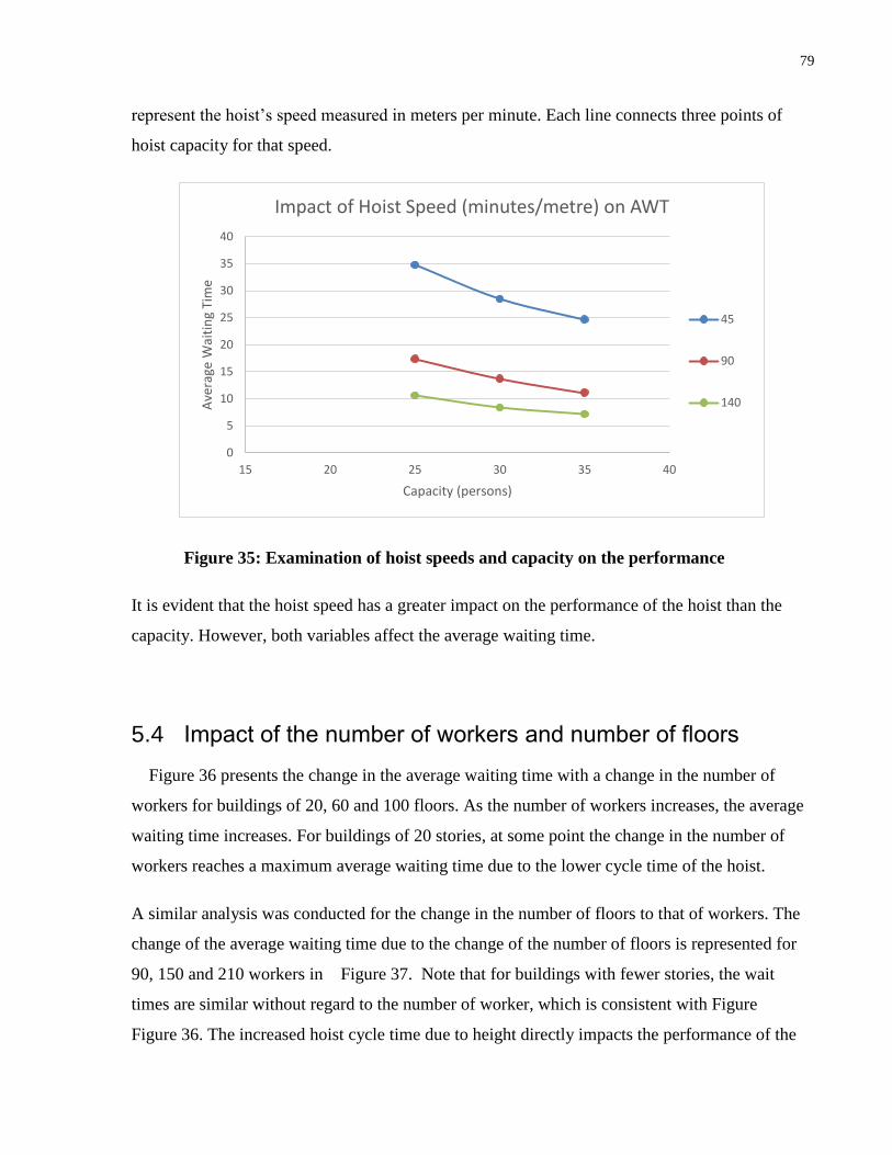
79
represent the hoist’s speed measured in meters per minute. Each line connects three points of
hoist capacity for that speed.
Figure 35: Examination of hoist speeds and capacity on the performance
It is evident that the hoist speed has a greater impact on the performance of the hoist than the
capacity. However, both variables affect the average waiting time.
5.4 Impact of the number of workers and number of floors
Figure 36 presents the change in the average waiting time with a change in the number of
workers for buildings of 20, 60 and 100 floors. As the number of workers increases, the average
waiting time increases. For buildings of 20 stories, at some point the change in the number of
workers reaches a maximum average waiting time due to the lower cycle time of the hoist.
A similar analysis was conducted for the change in the number of floors to that of workers. The
change of the average waiting time due to the change of the number of floors is represented for
90, 150 and 210 workers in Figure 37. Note that for buildings with fewer stories, the wait
times are similar without regard to the number of worker, which is consistent with Figure
Figure 36. The increased hoist cycle time due to height directly impacts the performance of the
0
5
10
15
20
25
30
35
40
15 20 25 30 35 40
Ave
rage
Wai
tin
g Ti
me
Capacity (persons)
Impact of Hoist Speed (minutes/metre) on AWT
45
90
140

80
hoist. This reaffirms the importance of improving the hoist operation as the buildings increase in
height.
Figure 36: Examination of the impact of the number of workers.
Figure 37: Examination of the impact of the number of floors
0
2
4
6
8
10
12
14
16
18
20
0 50 100 150 200 250
Ave
rage
Wai
tin
g ti
me
(min
s)
Number of Workers
Impact of Number of Workers by Number of Workers
100
60
20
0
5
10
15
20
25
30
0 20 40 60 80 100 120 140 160
Ave
rage
wai
tin
g ti
me
Number of Floors
Impact of Number of Floors
210
150
90
Number of
Workers
Number of
Floors

81
Figure 37 also suggests a linear function, so this analysis is provided to supplement
understanding of the impact of the number of floors on the average waiting time. Three
functions were investigated: linear, quadratic and power and they have the general formulas:
Equation 17 : Linear trend-line equation
𝑌 = 𝐴𝑥 + 𝐵
Equation 18: Quadratic trend-line equation
𝑌 = 𝐴𝑥2 + 𝐵𝑥 + 𝐶
Equation 19: Power trend-line equation
𝑌 = 𝐴𝑥𝐵 + 𝐶
Figures Figure 38, Figure 39 and Figure 40 demonstrate the fit of these functions. Using the R-
Squared parameter to compare the fits, it is evident that any of the three functions could
reasonably represent the relationship. However, by observing the trends, the linear function is not
a good representation for the lower values of the number of floors. Furthermore, the power
function deviates at the higher number of floors. The quadratic function provides the best fit for
the representation of this relationship. This suggests the large impact that the number of floors
has on the hoist productivity. Table 24 summarizes the R-Squared results with the best fit per
worker category bolded. The quadratic functions provide the best overall fit based on the R-
squared and on examination of the graphs.
Table 24: Summary of R-Squared values for different fits
Function R-Squared
90 workers 150 workers 210 workers
Linear 0.9532 0.9733 0.9764
Quadratic 0.9863 0.9806 0.9533
Power 0.9707 0.9655 0.9691
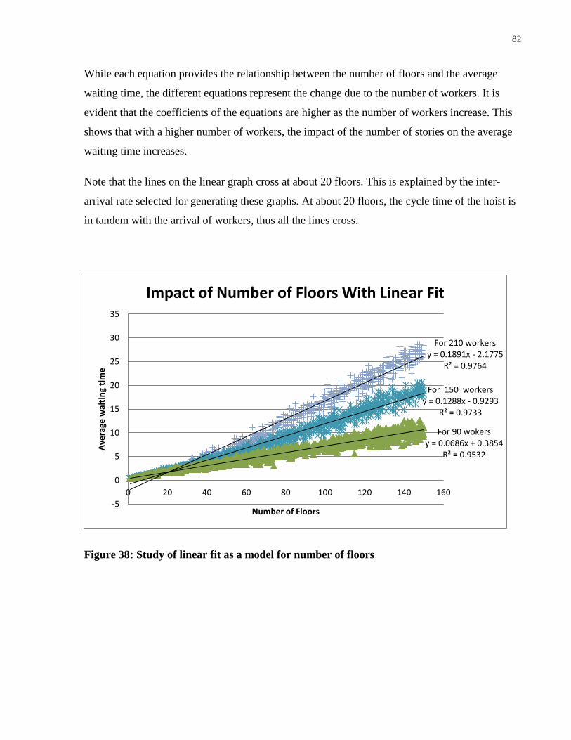
82
While each equation provides the relationship between the number of floors and the average
waiting time, the different equations represent the change due to the number of workers. It is
evident that the coefficients of the equations are higher as the number of workers increase. This
shows that with a higher number of workers, the impact of the number of stories on the average
waiting time increases.
Note that the lines on the linear graph cross at about 20 floors. This is explained by the inter-
arrival rate selected for generating these graphs. At about 20 floors, the cycle time of the hoist is
in tandem with the arrival of workers, thus all the lines cross.
Figure 38: Study of linear fit as a model for number of floors
For 210 workers y = 0.1891x - 2.1775
R² = 0.9764
For 150 workers y = 0.1288x - 0.9293
R² = 0.9733
For 90 wokers y = 0.0686x + 0.3854
R² = 0.9532
-5
0
5
10
15
20
25
30
35
0 20 40 60 80 100 120 140 160
Ave
rage
wai
tin
g ti
me
Number of Floors
Impact of Number of Floors With Linear Fit

83
Figure 39: Study of quadratic fit as a model for number of floors
Figure 40: Study of power fit as a model for number of floors
For 210 workers y = 0.0005x2 + 0.1138x - 0.34
R² = 0.9863
For 150 workers y = 0.0003x2 + 0.0853x + 0.1718
R² = 0.9806
For 90 workers y = 2E-05x2 + 0.0663x + 0.4406
R² = 0.9533
-5
0
5
10
15
20
25
30
0 20 40 60 80 100 120 140 160
Ave
rage
wai
tin
g ti
me
Number of Floors
Impact of Number of Floors With Quadratic Fit
For 210 workers y = 0.0931x1.1084
R² = 0.9707
For 150 workers y = 0.126x0.9724
R² = 0.9655
For 90 workers y = 0.1775x0.7992
R² = 0.9691
0
5
10
15
20
25
30
0 20 40 60 80 100 120 140 160
Ave
rage
wai
tin
g ti
me
Number of Floors
Impact of Number of Floors With Power Fit

84
Chapter 6 Using the Model to Improve Hoist Performance
6
This section provides the analysis of a hypothetical project to test the impact of two strategies on
the performance of the hoist. A tall building with 90 stories is considered with 230 workers and a
hoist capacity of 30 workers.
The hoist operating strategy will look at three schedules. Schedule A is where workers arrive all
at once at the start of the work day. Schedule B is where workers arrive individually throughout
one hour. For simplicity, this was modeled with equal interarrival times. For example, 230
workers arriving over one hour means that one worker arrives every 15.65 seconds or 0.26
minutes. In reality, this might represent cases where subcontractors first meet with their workers
for safety talks before going up to work, thereby delaying their arrival at the hoist. Finally,
Schedule C represents zoning and staggered starts, where the floors are separated into 5 zones
and workers who are scheduled to work on the higher zones are taken their first (zoning) or
arrive earlier (staggered starts). The groups represent the work underway at each level such as
formwork, electrical and plumping. The number and destination of the workers was developed
using expert opinion. Table 25 summarizes the variables and Table 26 summarizes the arrival
schedules.
Table 25: Inputs used in the analysis
Case 1 2 3 4 5 6 7
Arrival Schedule (described in Table 26) A A B B C
0
min
C
15
min
C
20
min
Hoist Travel Time per Floor (min.) 0.04 0.025 0.04 0.025 0.04 0.04 0.04
Number of Floors 90
Number of Workers 230
Hoist Capacity (people) 30
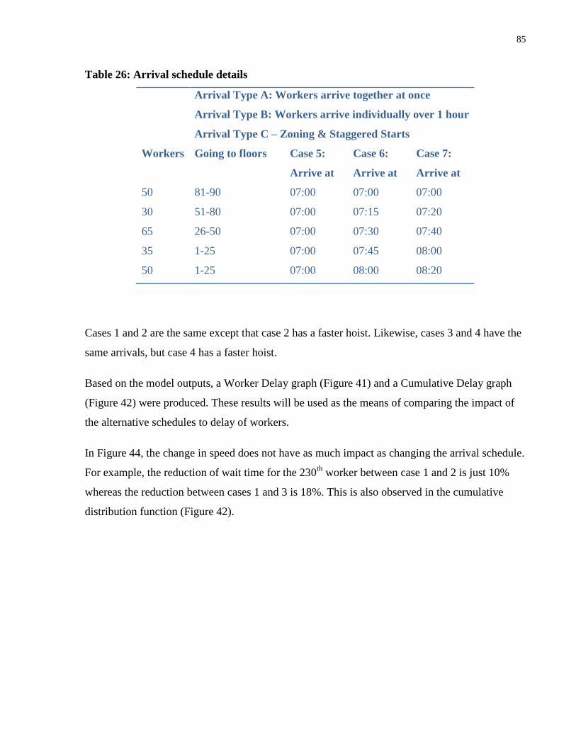
85
Table 26: Arrival schedule details
Arrival Type A: Workers arrive together at once
Arrival Type B: Workers arrive individually over 1 hour
Arrival Type C – Zoning & Staggered Starts
Workers Going to floors Case 5:
Arrive at
Case 6:
Arrive at
Case 7:
Arrive at
50 81-90 07:00 07:00 07:00
30 51-80 07:00 07:15 07:20
65 26-50 07:00 07:30 07:40
35 1-25 07:00 07:45 08:00
50 1-25 07:00 08:00 08:20
Cases 1 and 2 are the same except that case 2 has a faster hoist. Likewise, cases 3 and 4 have the
same arrivals, but case 4 has a faster hoist.
Based on the model outputs, a Worker Delay graph (Figure 41) and a Cumulative Delay graph
(Figure 42) were produced. These results will be used as the means of comparing the impact of
the alternative schedules to delay of workers.
In Figure 44, the change in speed does not have as much impact as changing the arrival schedule.
For example, the reduction of wait time for the 230th
worker between case 1 and 2 is just 10%
whereas the reduction between cases 1 and 3 is 18%. This is also observed in the cumulative
distribution function (Figure 42).

86
Figure 41: Results showing worker arrival cases using the delay graph.
Case 1- arrive together and slower hoist Case 5- arrive together and zoning
Case 2-arrive together and faster hoist Case 6- staggered starts (15 minute intervals)
Case 3-arrive individually and slower hoist Case 7- staggered starts (20 minute intervals)
Case 4- arrive individually and faster hoist Cases 5, 6, and 7 use the faster hoist
-20
0
20
40
60
80
100
120
0 30 60 90 120 150 180 210
Wai
tin
g Ti
me
(m
ins)
Worker in order of arrival
Delay per worker
1
2
3
4
5
6
7

87
Figure 42: Results showing worker arrival cases using the cumulative distribution.
Case 1- arrive together and slower hoist Case 5- arrive together and zoning
Case 2-arrive together and faster hoist Case 6- staggered starts (15 minute intervals)
Case 3-arrive individually and slower hoist Case 7- staggered starts (20 minute intervals)
Case 4- arrive individually and faster hoist Cases 5, 6, and 7 use the faster hoist
Scheduling workers according to their destination is a novel strategy in hoist planning. In the
cases where the workers arrive together at the beginning of the shift, there is an improvement
attained from just zoning. However, this improvement is not as significant as the cases where the
workers from each zone are scheduled to arrive at different times. Case 5 demonstrates that while
zoning has a 20% reduction in the waiting time of the 230th
worker in comparison to case 1, the
reduction attained from case 6 (combination of staggered arrivals and zoning) has a reduction of
about 85%. Figure 43 highlights these reductions in waiting times.
0.00%
10.00%
20.00%
30.00%
40.00%
50.00%
60.00%
70.00%
80.00%
90.00%
100.00%
110.00%
0 20 40 60 80 100
Pe
rce
nt
of
Wo
rke
rs
Waiting Time (mins)
Percent Waiting
1
2
3
4
5
6
7

88
Figure 43: Highlighting the impact of the Zoning on the hoist performance.
Case 1- arrive together and slower hoist Case 4- arrive individually and faster hoist
Case 6- staggered starts (15 minute intervals and faster hoist )
In the cases where the workers arrive at once and over one hour (schedules A and B), there is an
increasing trend of waiting time. While cases 3, 4 and 6 all have the workers arrive within one
hour, scheduling staggering starts as in case 6 greatly reduces the waiting times of the workers.
This comparison is highlighted in Figure 44.
-20
0
20
40
60
80
100
120
0 30 60 90 120 150 180 210
Wai
tin
g Ti
me
(m
ins)
Worker in order of arrival
Delay per worker
1
4
6

89
Figure 44: Highlighting the impact of the alternative strategy over one hour arrival time.
Case 3-arrive individually and slower hoist Case 5- arrive together and zoning
Case 6- staggered starts (15 minute intervals and faster hoist )
Table 27, demonstrates the benefit of the proposed scheduling strategy by comparing the delay
of 80% and 50% of workers in the cumulative graph.
Staggered starts in 15 min intervals (case 6) as opposed to having workers start at once (case 1)
reduces the 80th
percentile wait by over one hour and 45 minutes by the 50% percentile. The
specific schedule would depend upon the stage of construction, the local practices and/or
regulations, and the ability of the site manager to affect the working schedule of the
subcontractors. However, the opportunity to reduce wait times should be very appealing to
subcontractors.
-10
0
10
20
30
40
50
60
70
80
0 30 60 90 120 150 180 210
Wai
tin
g Ti
me
(m
ins)
Worder in order of arrival
Delay per worker
3
5
6

90
Table 27: Cumulative delay for 50% and 80% of workers
Case Cumulative delay for the 50th
percentile of workers (mins)
Cumulative delay for 80th
percentile of workers (mins)
1 51 79
2 45 71
3 29 46
4 21 36
5 38 58
6 6 11
7 0 4
In conclusion, this study demonstrates the opportunity of using the proposed staggered starts
strategy for the improvement of the hoist productivity.

91
Chapter 7 Conclusion and Recommendations
7
This chapter summarizes the contributions of this research, its limitations, and recommendations
for future research.
7.1 Conclusions
Tall buildings are becoming more common in North America, including in the Toronto area. The
challenges of moving resources vertically for tall buildings are based upon the increase of wind
speeds, longer travel times and limited space for the construction in the city. This research
examined the effectiveness of hoist operations and its effect on worker delays.
A comprehensive overview of the previous efforts to study hoists was presented. However, due
to the scarcity of studies that looked at the hoist, research that studies elevators was also
reviewed. It was observed that previous efforts to study hoists had limitations. First, a large
number of inputs are needed by some of the models. Second, the measures of hoist performance
do not necessarily reflect the domino effect of hoist operations. Finally the way in which workers
arrive to the site has not been studied, which has been a common factor in elevators.
A discrete-event simulation (DES) model was developed for this project. DES provides a
mechanism to model complex systems and of accounting for statistical variability.
To develop the model, data from site observations and expert opinion were collected to represent
the transportation of workers during the morning up-peak. The inputs required by the model
were limited to factors that have a high impact on the output. Also, the way in which workers
arrive to the site in the morning was studied and included in the model. Finally, the model
provides three outputs: average waiting time, delay graph and cumulative delay distribution to
represent the performance of the hoist. The average waiting time is a common decision variable
that has been used in elevator planning, but has not yet been adapted to hoists. The model was
verified and validated. The results show that the model’s output is reflective of the operation of
the hoist.

92
An analysis of the impact of the factors on the performance of the hoist has been conducted. It is
evident that each of the factors has an influence on the hoist’s performance. Furthermore, an
application for the model to improve hoist performance was undertaken to study the impact of
the alternative scheduling strategy on the delay of workers. It was concluded that scheduling
staggered starts for the workers in accordance to their location of work provides a significant
improvement to the hoist’s productivity.
The object of this study was to optimize hoist performance for high-rise building construction,
enabling an efficient delivery of workers during the morning peak. The impact of staggered
arrivals and zoning on the performance of the hoist provides a solution and meets the objective
of the study.
7.2 Limitations of the study
Provided the scope and assumptions of this study, a few limitations arise. The limitations of this
study are as follows:
This study is limited to the delivery of workers. However, the hoist may be used for the
delivery of materials. Therefore, in situations where the hoist is being used for both
materials and workers, the model is not reflective of the hoist operation.
The wind speeds as a building gets higher may cause malfunctions in the hoist. The hoist
might operate at lower speeds or completely shut-down. This study did not take these
situations into consideration.
Some site activities during the morning peak may not be reflected in the model. For
example, if there is inter-floor travel or if workers are using the hoist to return to the
ground floor during the morning peak.
The hoist operator’s characteristics, such as skill or experience, have not been considered
in this study.
The different hoist technologies have not been taken into account. A self-leveling hoist or
hoists with an automatic control system may produce productivity improvements.

93
The staggered starts strategy has not been validated using data collected from site as it
has not been tried. Therefore, the performance of the hoist in these idealistic situations
may be altered by factors which have not been taken into consideration.
The operation of the building’s elevators has not been taken into account as it is assumed
that they are not yet available for use.
7.3 Recommendations
This study provides a starting point for many possible future endeavours to further research hoist
operations and improving hoist productivity. Some of the aspects that future researchers may
undertake are:
The model focused on the delivery of workers in the morning. While this aspect is
commonly used in elevators, the delivery of material is specific to hoists. Therefore, the
model could be expanded to include the delivery of materials. Furthermore, the model
may also be extended to different times of day and to model construction progress
throughout the project. This requires the addition of the inter-floor travel, travel during
breaks and the end of the shift, along with the delivery of materials.
Aspects that have an influence on the performance of the hoist include new hoist
technologies, location of the hoist and platform design. Future research may study the
impact of these factors on the performance of the hoist. The use of a self-leveling hoist,
for example, may be an aspect which improves the hoist performance. Additionally, the
location of the hoist and the platform design may influence the loading and unloading
times of the hoist.
The study of the hoist operation using different methods may provide more insight on
ways of improving the hoist’s performance. The analysis of this study suggests that a
linear regression may be used to represent the hoist’s operation. Moreover, artificial
intelligence methods could be an alternative method of analysis.
An automated method for inputting the information into the model, and providing an
output may be developed to make the model more user-friendly.

94
For the purpose of decision-makers, graphical representation in the form of design graphs
for different situations may be created. This would make the decision making process
easier and faster. The graphical format is more industry-friendly and does not require
knowledge in DES.

95
Bibliography
AbouRizk, S. (2014). NSERC Industrial Chair, Construction Management and Engineering,
Software. Retrieved from University of Alberta:
http://irc.construction.ualberta.ca/en/Research/ChairProfile/Software.aspx
AbouRizk, S. (2014). "Simphony.Net: An integrated enviroment for construction simulation."
NSERC IRC in Construction Engineering and Managmenet-Simulation:Simphony, 12.
Ahuja, H., Dozzi, S., and AbouRizk, S. (1994). "Project Management Techniques in Planning
and Controlling Construction Projects." New York: Wiley & Sons Inc.
Altiok, T., and Melamed, B. (2007). "Simulation Modeling and Analysis with ARENA." Elsevier.
Arora, J. S. (2012). "Introduction to Optimum Design, Third Edition." San Diego, San Fraciso,
Singapore, Sydney, Tokyo: Elsevier.
Banks, J. (1998). "Handbook of Simulation: Principles, Methodology, Advances, Application and
Practice." New York: John Wiley & Sons, Inc.
Barney, G. C., and Santos, S. M. (1975). "Improved Traffic Design Methods for Lift Systems."
Building Science, 277-285.
Belegundu, A. D., and Chandrupatla, T. R. (2011). "Optimization Concepts and Applications in
Engineering (2nd Edition)." New York: Cambridge University Press.
Benmakhlouf, S. M., and Khator, S. K. (1993). "Smart Lifts: Control Design and Performance
Evaluation." Computers and Industrial Engineering, 175-178.
Bigge Crane and Rigging Company. (2014). "Construction Hoist Rental." Retrieved from Bigge
Crane and Rigging Co.: http://www.biggetowercrane.com/construction-hoists.html
Bingham, N. H., and Fry, J. M. (2010). "Regression-Linear Models in Statistics." London:
Springer-Verlag.

96
Brown, W. M., and Newbold, K. B. (2012). "Cities and Growth: Moving to Toronto –Income
Gains Associated with Large Metropolitan Labour Markets." Statistics Canada-Economic
Analysis Division.
Chang, D. (1987). "RESQUE PhD Thesis." University of Michigan: Ann Arbor, Michighan
Chen, H.-M., and Huang, P.-H. (2013). "3D AR-Based Modeling for Discrete-Event Simulation
of Transport Operations in Construction." Automation in Construction, 123-136.
Cho, C.-Y., Cho, M.-Y., Kim, Y.-S., Kim, J. Y., Lee, J. B., and Kwon, S.-W. (2010).
"Simulation Method of Construction Hoist Operating Plan for High Rise Buildings
Considering Lifting Heights and Loads." 27th International Symposium on Automation
and Robotics in Construction, 22-28.
Cho, C.-Y., Kwon, S., Shin, T.-H., Chin, S., and Kim, Y.-S. (2011). "A Development of Next
Generation Intelligent Construction Liftcar Toolkit for Vertical Material Movement
Management." Automation in Construction, 14-27.
Cho, C.-Y., Yoosub, L., Cho, M.-Y., Kwon, S., Shin, Y., and Lee, J. (2013). "An Optimal
Algorithm of the Multi-Lifting Operating Simulation for Super-Tall Building
Construction." Automation in Construction, 595-607.
Christodoulou, S., Ellinas, G., and Aslani, P. (2009). "Entropy-Based Scheduling of Resource-
Constrained Construction Projects." Automation in Construction, 919-928.
CIBSE. (1993). "CIBSE Guide D,Transportation Systems in Buildings." The Chartered
Institution of Building Services Engineers.
Cortés, P., Larrañeta, J., and Onieva, L. (2004). "Genetic Algorithm for Controllers in Elevator
Groups: Analysis and Simulation During Lunchpeak Traffic." Applied Soft Computing,
159-174.
CTBUH . (2014). CTBUH Height Criteria. Retrieved from Council on Tall Buildings and Urban
Habitat:
http://www.ctbuh.org/HighRiseInfo/TallestDatabase/Criteria/tabid/446/language/en-
GB/Default.aspx

97
CTBUH. (2011). "2013: A Tall Building Review." CTBUH Journal, 1-2.
CTBUH. (2012). "Canada Grows Taller." CTBUH Journal, 2-3.
de Neufville, R., and Scholtes, S. (2011). "Flexibility in Engineering Design." Cambridge,
Massachuetts, London: MIT Press.
Devor, J. L. (2009). "Probability amd Statistics For Engineering and the Sciences." Belmont:
Brooks/Cole.
Dozzi, S., and AbouRizk, S. (1993). "Productivity in Construction." Ottawa: National Research
Council Canada.
Gautschi, W. (2012). "Numerical Analysis, Second Edition ." New York,Dordrecht,
Heidelberg,London: Springer Science+Business Media.
Hajjar, D., and AbouRizk, S. (1999). "Simphony: An Environment for Building Special Purpose
Construction Simulation Tools." Proceedings of the Winter Simulation Conference,
Phoenix, Arizona, 998-1006.
Hajjar, D., and AbouRizk, S. (2002). "Unified Modeling Methodology for Construction
Simulation." Journal of Construction Engineering and Managment, 174-185.
Halpin, D., and Riggs, L. (1992). "Planning and Analysis of Construction Operations." Canada:
John Wiley & Sons, Inc.
Hauser, J. R. (2009). "Numerical Methods for Nonlinear Engineering Models." Dordrecht:
Springer Science+ Business Media.
Hwang, S. (2009). "Planning Temporary Hoists for Building Construction." Construction
Research Congress, 1300-1307.
Ioannou, P. (1989). "UM_CYCLONE." Dept. of Civil Engineering, University of Michigan: Ann
Arbor, Michigan

98
Ioannou, P. G., and Martinez, J. C. (1996). "Comparison of Construction Alternatives Using
Matched Simulation Experiments." Journal of Construction Engineering and
Management, 231-241.
Ioannou, P. G., and Martinez, J. C. (1996). "Scalable Simulation Models for Construction
Operations." Proceedings of the 1996 Winter Simulation Conference , 1329-1336.
Ladany, S. P., and Hersh, M. (1979). "The Design of an Efficient Elevator Operating." European
Journal of Operational Research, 216-221.
Levitt, R. E., Thomsen, J., Christiansen, T. R., Kunz, J. C., Jin, Y., and Nass, C. (1999).
"Simulating Project Work Processes and Organizations: Toward a Micro-Contingency
Theory of Organizational Design." Management Science, 1479-1495.
Martinez, J. C. (1996). "STROBOSCOPE: State and Resource Based Simulation of Construction
Processes." Ph.D. Dissertation, University of Michigan: Ann Arbor, Michigan
Martinez, J. C. (2010). "Methodology for Conducting Discrete-Event Simulation Studies in
Construction Engineering and Management." Journal of Construction Engineering and
Management, 3-16.
McDonough Elevators . (2013). "Construction Hoist Rental ." Retrieved from McDonough
Elevators : http://www.mcdelevators.com/construction-hoist-rental.html
Metro Elevator. (2013). "Construction Hoists for lease ." Retrieved from Metro Elevator:
http://metroelevator.com/construction-hoists-lease
Monahan, J. F. (2001). "Numerical Methods of Statistics." Cambridge: Cambridge University
Press.
Mooney, C. Z. (1997). "Monte Carlo Simulation." Thousands Oaks, CA: SAGE publications,
Inc.
Nagatani, T. (2003). "Complex Behavior of Elevators in Peak Traffic." Physica A, 556-566.
Nagatani, T. (2004). "Dynamical Transitions in Peak Elevator Traffic." Physica A, 441-452.

99
Naylor, T. J., Balintfy, J. L., Burdick, D. S., and Chu, K. (1996). "Computer Simulation
Techniques." New Work: John Wiley & Sons.
Nelson, P. R., Coffin, M., and Copeland, K. A. (2003). "Introductory Statistics for Engineering
Experimentation." Online : Elsevier.
Park, M., Ha, S., Lee, H.-S., Choi, Y.-k., Kim, H., and Han, S. (2013). "Lifting Demand-Based
Zoning for Minimizing Worker Vertical Transportation Time in High-Rise Building
Construction." Automation in Construction, 88-95.
Paulson, B. J. (1978). "Interactive Graphics for Simulating Construction Operations." Journal of
Construction Div., 69-76.
Peters, R. (2014). Elevate. Retrieved from Peters Research: https://www.peters-
research.com/index.php/elevate
Puri, V., and Martinez, J. C. (2013). "Modeling of Simultaneously Continuous and Stochastic
Construction Activities for Simulation." Journal of Construction Engineering and
Management, 1037-1045.
Raychaudhuri, S. (2008). "Introduction to Monte Carlo Simulation ." Proceedings of the 2008
Winter Simulation Conference, 91-100.
Ross, S. M. (2013). "Simulation (Fifth Edition)." Amesterdam, Boston, Hidelberg, London, New
York, Oxford, Paris, San Daiego, San Francisco, Singapore, Sydney, Tokyo: Elsevier Inc.
Rubinstein, R. Y., and Kroese, D. P. (2007). "Simulation and the Monte Carlo Method, Second
Edition." Hoboken, New Jersey: John Wiley & Sons, Inc.
Ruwanpura, J. Y., and Ariaratnam, S. T. (2007). "Simulation Modeling Techniques for
Underground Infrastructure Construction Processes." Tunnelling and Underground Space
Technology, 553-567.
Shi, J. (1997). "A Conceptual Activity Cycle-Based Simulation Modeling Method." Proceedings
of the 1997 Winter Simulation Conference, 1127-1133.

100
Shin, Y., Cho, H., and Kang, K.-I. (2011). "Simulation Model Incorporating Genetic Algorithms
for Optimal Temporary Hoist Planning in High-Rise Building Construction." Automation
in Construction, 550-558.
Skyscraper Center . (2014). Interactive Data. Retrieved from Skyscraper Center- The Global
Tall Building Database of the CTBUH: http://skyscrapercenter.com
Soekiman, A., Pribadi, K., Soemardi, B., and Wirahadikusuman, R. (2011). "Factors Relating to
Labor Productivity Affecting the Project Schedule Performance in Indonesia." Procedia
Engineering, 865–873.
Statistics Canada. (2014, 04 30). "CANSIM." Gross domestic product at basic prices, by
industry (monthly). Canada. Retrieved 05 12, 2014, from http://www.statcan.gc.ca/tables-
tableaux/sum-som/l01/cst01/gdps04a-eng.htm
Tervonena, T., Lahdelmabr, R., and Hakonen, H. (2008). "Elevator Planning with Stochastic
Multicriteria Acceptability Analysis." Omega, 352-362.
Thomas, H. R. (1991). "Labor Productivity and Work Sampling: The Bottom Line." Journal of
Construction Engineering and Management, 423-444.
Tommelein, I., and Odeh, A. (1994). "Knowledge-Based Assembly of Simulation Networks
Using Construction Designs, Plans and Methods." Proceedings of the 1994 Winter
Simulation Conference, 1145-1158.
USA Hoist. (2014). "Construction Hoisting ." Retrieved from USA Hoist : www.usahoist.com
Zuppa, D. (2014, 01 07). Construction . Retrieved from National Research Council Canada :
http://www.nrc-cnrc.gc.ca/eng/rd/construction/index.html

101
Appendices
Appendix 1: References on Artificial Intelligence
1. Comprehensive Materials processing by Dobrzanski, Trzaska, Dobrzanska-Danikiewicz
2. Artificial intelligence Foundations of Computational Agents by David Poole and Alan
Mackworth
3. Artificial Intelligence and Expert Systems by Y. Leung
4. Artificial Intelligence; A Modern Approach by Stewart J. Russell and Peter Norvig
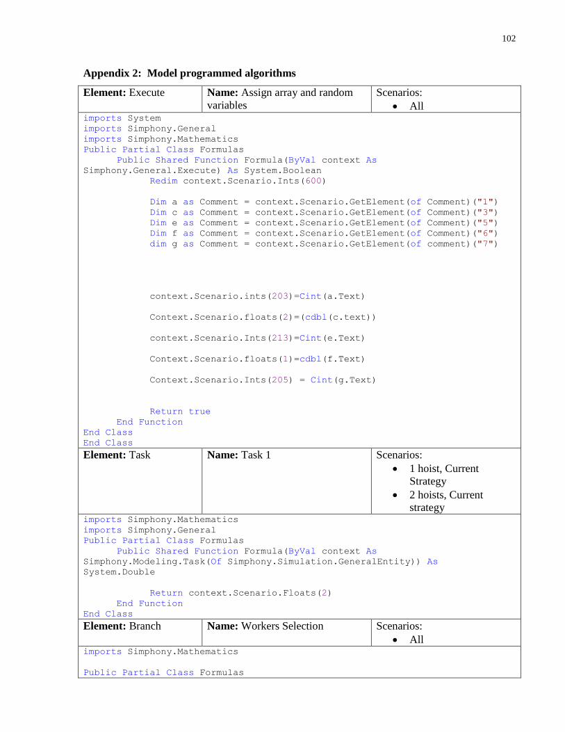
102
Appendix 2: Model programmed algorithms
Element: Execute Name: Assign array and random
variables
Scenarios:
All imports System
imports Simphony.General
imports Simphony.Mathematics
Public Partial Class Formulas
Public Shared Function Formula(ByVal context As
Simphony.General.Execute) As System.Boolean
Redim context.Scenario.Ints(600)
Dim a as Comment = context.Scenario.GetElement(of Comment)("1")
Dim c as Comment = context.Scenario.GetElement(of Comment)("3")
Dim e as Comment = context.Scenario.GetElement(of Comment)("5")
Dim f as Comment = context.Scenario.GetElement(of Comment)("6")
dim g as Comment = context.Scenario.GetElement(of comment)("7")
context.Scenario.ints(203)=Cint(a.Text)
Context.Scenario.floats(2)=(cdbl(c.text))
context.Scenario.Ints(213)=Cint(e.Text)
Context.Scenario.floats(1)=cdbl(f.Text)
Context.Scenario.Ints(205) = Cint(g.Text)
Return true
End Function
End Class
End Class
Element: Task Name: Task 1 Scenarios:
1 hoist, Current
Strategy
2 hoists, Current
strategy imports Simphony.Mathematics
imports Simphony.General
Public Partial Class Formulas
Public Shared Function Formula(ByVal context As
Simphony.Modeling.Task(Of Simphony.Simulation.GeneralEntity)) As
System.Double
Return context.Scenario.Floats(2)
End Function
End Class
Element: Branch Name: Workers Selection Scenarios:
All imports Simphony.Mathematics
Public Partial Class Formulas

103
Public Shared Function Formula(ByVal context As
Simphony.General.Branch) As System.Boolean
context.Scenario.Ints(204)= context.Scenario.Ints(204)+1
if context.Scenario.ints(204)<= context.Scenario.ints(203)then
return false
end if
return true
End Function
End Class
Element: Branch Name: Is hoist one available? Scenarios:
All Imports Simphony.General
imports Simphony.Mathematics
Public Partial Class Formulas
Public Shared Function Formula(ByVal context As
Simphony.General.Branch) As System.Boolean
Dim e As Resource = context.Scenario.GetElement(Of Resource)("Hoist1")
If e.Available > 0
Return true
end if
Return false
End function
End Class
Element: Branch Name: Is hoist two Available Scenarios:
2 Hoists, Current
Strategy
2 Hoists, Alternative
Strategy Imports Simphony.General
Public Partial Class Formulas
Public Shared Function Formula(ByVal context As
Simphony.General.Branch) As System.Boolean
Dim e As Resource = context.Scenario.GetElement(Of Resource)("Hoist1")
Dim f As Resource = context.Scenario.GetElement(Of Resource)("Hoist2")
if f.Available> 0
Return true
end if
Return false
End function
End Class
Element: Branch Name: No Hoist Available Scenarios:
2 Hoists, Current
Strategy
2 Hoists, Alternative
Strategy Imports Simphony.General

104
Public Partial Class Formulas
Public Shared Function Formula(ByVal context As
Simphony.General.Branch) As System.Boolean
Dim e As Resource = context.Scenario.GetElement(Of Resource)("Hoist1")
Dim f As Resource = context.Scenario.GetElement(Of Resource)("Hoist2")
if f.Available> 0
Return true
end if
Return false
End function
End Class
Element: Branch Name: Capacity Reached? Scenarios:
All Public Partial Class Formulas
Public Shared Function Formula(ByVal context As
Simphony.General.Branch) As System.Boolean
if context.CurrentEntity.Floats(2)-context.Engine.TimeNow > 1
then
return false
end if
context.Scenario.Ints(200) = context.Scenario.Ints(200) + 1
if context.Scenario.Ints(200) < (context.Scenario.Ints(205)*0.8)
then
Return true
End if
Return False
Element: Execute Name: Number of Stops Scenarios:
All Public Partial Class Formulas
Public Shared Function Formula(ByVal context As
Simphony.General.Execute) As System.Boolean
Context.Scenario.Ints(context.CurrentEntity.Ints(0))=Context.Scenario.I
nts(context.CurrentEntity.Ints(0))+1
Return true
End Function
End Class
Element: Execute Name: Last Stop Scenarios:
All Public Partial Class Formulas
Public Shared Function Formula(ByVal context As
Simphony.General.Execute) As System.Boolean
If context.CurrentEntity.Ints(0)> context.Scenario.Ints(201) then

105
Context.Scenario.Ints(201) = context.CurrentEntity.Ints(0)
End if
Return True
End Function
End Class
Element: Execute Name: Calculation Scenarios:
All Public Partial Class Formulas
Public Shared Function Formula(ByVal context As
Simphony.General.Execute) As System.Boolean
context.Scenario.Floats(5) = context.Scenario.Floats(5)+
context.CurrentEntity.Floats(1)
if context.CurrentEntity.Floats(1)>
context.Scenario.Floats(3) then
context.Scenario.Floats(3)= context.CurrentEntity.Floats(1)
end if
If context.CurrentEntity.Ints(0)> context.Scenario.Ints(212) then
Context.Scenario.Ints(212) = context.CurrentEntity.Ints(0)
End if
Return true
End Function
End Class
Element: Chart Collect Name: ChartCollect Scenarios:
All
X-Value imports Simphony.General
Public Partial Class Formulas
Public Shared Function Formula(ByVal context As
Simphony.General.ChartCollect) As System.Double
Dim e as Counter = context.Scenario.GetElement(of
Counter)("numberofworkers")
Return e.Count
End Function
End Class
Y-Value Public Partial Class Formulas
Public Shared Function Formula(ByVal context As
Simphony.General.ChartCollect) As System.Double
Return context.CurrentEntity.Floats(1)
End Function
End Class

106
Element: Statistic
Collect
Name: StatisticsCollect Scenarios:
All
Public Partial Class Formulas
Public Shared Function Formula(ByVal context As
Simphony.General.Collect) As System.Double
Return context.CurrentEntity.Floats(1)
End Function
End Class
Element: Branch Name: Branch 2 Scenarios:
All
imports Simphony.General
Public Partial Class Formulas
Public Shared Function Formula(ByVal context As
Simphony.General.Branch) As System.Boolean
Dim a as Counter = context.Scenario.GetElement(of
Counter)("numberofworkers")
If a.count< context.Scenario.Ints(203) then
return true
End if
Return false
End Function
End Class
Element: Execute Name: Average Waiting Time Scenarios:
All
imports Simphony.Mathematics
Public Partial Class Formulas
Public Shared Function Formula(ByVal context As
Simphony.General.Execute) As System.Boolean
Context.Scenario.Floats(6) =
(Context.Scenario.Floats(5)/context.Scenario.Ints(203))
Return true
End Function
End Class
Element: Trace Name: Data Scenarios:
All
Public Partial Class Formulas

107
Public Shared Function Formula(ByVal context As Simphony.General.Trace)
As System.String
Dim numofhoist as Integer
Select case context.Scenario.Name
Case "1 Hoist-CS"
numofhoist = 1
Case "2 hoists-CS"
numofhoist= 2
End select
Return" |Senario| "& context.Scenario.name & " |numofhoists| "
&Cstr(numofhoist) &" |no. of workers-Actual| "&
Cstr(Context.Scenario.Ints(203))& " |Average Arrival interval| "&
Cstr(context.scenario.floats(2)/2)&" |no. of stories| "&
Cstr(Context.Scenario.Ints(213))&" |timeperfloor| "&
Cstr(context.Scenario.floats(1))&" |Capacity| "&
Cstr(context.Scenario.Ints(205))&" |Avg Wating time| "&
Cstr(context.Scenario.floats(6))&" |Max Wating time| "&
Cstr(context.Scenario.floats(3))
End Function
End Class
Element: Execute Name: Assign Hoist Number Scenarios:
All
Public Partial Class Formulas
Public Shared Function Formula(ByVal context As
Simphony.General.Execute) As System.Boolean
context.scenario.ints(211)= context.scenario.ints(211)+ 1
Context.currententity.Ints(2)= context.scenario.ints(211)
Return true
End Function
End Class
Element: Branch Name: Hoist 1 or 2 Scenarios:
All
Public Partial Class Formulas
Public Shared Function Formula(ByVal context As
Simphony.General.Branch) As System.Boolean
If context.CurrentEntity.Ints(2) = 1 then
Return true
end if
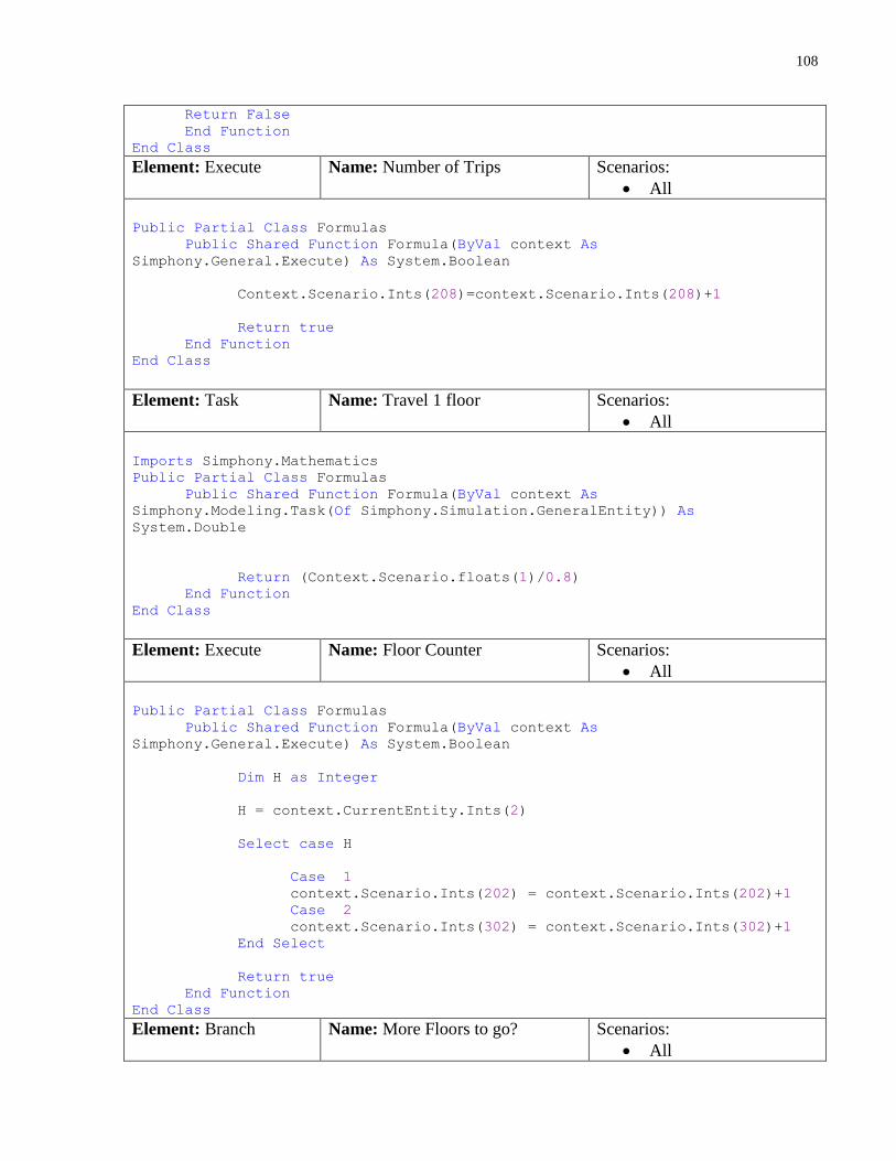
108
Return False
End Function
End Class
Element: Execute Name: Number of Trips Scenarios:
All
Public Partial Class Formulas
Public Shared Function Formula(ByVal context As
Simphony.General.Execute) As System.Boolean
Context.Scenario.Ints(208)=context.Scenario.Ints(208)+1
Return true
End Function
End Class
Element: Task Name: Travel 1 floor Scenarios:
All
Imports Simphony.Mathematics
Public Partial Class Formulas
Public Shared Function Formula(ByVal context As
Simphony.Modeling.Task(Of Simphony.Simulation.GeneralEntity)) As
System.Double
Return (Context.Scenario.floats(1)/0.8)
End Function
End Class
Element: Execute Name: Floor Counter Scenarios:
All
Public Partial Class Formulas
Public Shared Function Formula(ByVal context As
Simphony.General.Execute) As System.Boolean
Dim H as Integer
H = context.CurrentEntity.Ints(2)
Select case H
Case 1
context.Scenario.Ints(202) = context.Scenario.Ints(202)+1
Case 2
context.Scenario.Ints(302) = context.Scenario.Ints(302)+1
End Select
Return true
End Function
End Class
Element: Branch Name: More Floors to go? Scenarios:
All

109
Public Partial Class Formulas
Public Shared Function Formula(ByVal context As
Simphony.General.Branch) As System.Boolean
Dim H as Integer
H = context.CurrentEntity.Ints(2)
Select case H
Case 1
If context.Scenario.Ints(201) = Context.Scenario.Ints(202) then
Return false
End if
Case 2
if context.Scenario.Ints(301) = context.Scenario.Ints(302)
then
Return False
End If
End Select
Return true
End Function
End Class
Element: Branch Name: Stop on current floor? Scenarios:
All
Imports Simphony.General
Public Partial Class Formulas
Public Shared Function Formula(ByVal context As
Simphony.General.Branch) As System.Boolean
Dim H as Integer
H = context.CurrentEntity.Ints(2)
Select case H
Case 1
If context.Scenario.Ints(Context.Scenario.Ints(202))> 0
then 'there is a stop
context.Scenario.Ints(Context.Scenario.Ints(202))=0
return true
End if
Case 2
If context.Scenario.Ints(400+Context.Scenario.Ints(302))> 0
then 'there is a stop
context.Scenario.Ints(400+Context.Scenario.Ints(302))=0
return true
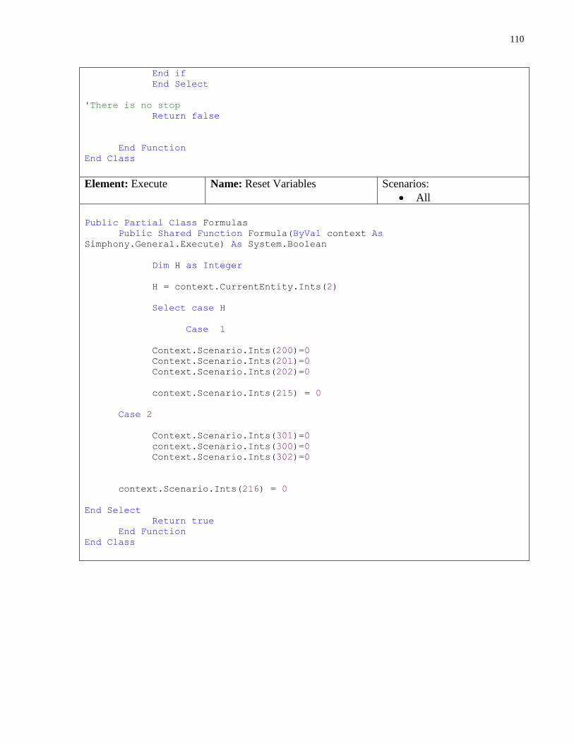
110
End if
End Select
'There is no stop
Return false
End Function
End Class
Element: Execute Name: Reset Variables Scenarios:
All
Public Partial Class Formulas
Public Shared Function Formula(ByVal context As
Simphony.General.Execute) As System.Boolean
Dim H as Integer
H = context.CurrentEntity.Ints(2)
Select case H
Case 1
Context.Scenario.Ints(200)=0
Context.Scenario.Ints(201)=0
Context.Scenario.Ints(202)=0
context.Scenario.Ints(215) = 0
Case 2
Context.Scenario.Ints(301)=0
context.Scenario.Ints(300)=0
Context.Scenario.Ints(302)=0
context.Scenario.Ints(216) = 0
End Select
Return true
End Function
End Class