improving efficiency of order picking in picker to …
TRANSCRIPT

IMPROVING EFFICIENCY OF ORDER PICKING
IN PICKER-TO-PARTS
WAREHOUSES
by
Moayad Khalil
Submitted in partial fulfilment of the requirements
for the degree of Master of Applied Science
at
Dalhousie University
Halifax, Nova Scotia
November 2013
© Copyright by Moayad Khalil, 2013

ii
Dedicated to
my dear parents Wajdi, & Ohood
and my lovely brothers, Moaad & Muthafer

iii
Table of Contents
List of Tables ......................................................................................................................................... v
List of Figures ....................................................................................................................................... vi
Abstract ................................................................................................................................................ vii
Acknowledgements ............................................................................................................................. viii
Chapter 1 - Introduction ....................................................................................................................... 1
Chapter 2 -Thesis Motivation ............................................................................................................... 5
2.1 Organization of the Thesis Report .......................................................................................... 6
Chapter 3 - Literature Review ............................................................................................................. 7
3.1 Improving Efficiency of Order Picking in Picker-to-parts Warehouses ................................. 7
3.1.1 The Full-turnover and The Nearest-location Storage Policies ..................................... 12
3.1.1.1 Travel Distance Estimation ...................................................................................... 15
3.2 Summary ............................................................................................................................... 17
Chapter 4 - Methodology .................................................................................................................... 19
4.1 Items Attributes .................................................................................................................... 19
4.2 Warehouse Layout Structure ................................................................................................ 20
4.2.1 Selection of Feasible Warehouse Layouts .................................................................... 21
4.3 Routing of Order Pickers ...................................................................................................... 22
4.4 Storage Assignment Policies ................................................................................................ 23
4.4.1 Full-turnover Storage Assignment Policy .................................................................... 24
4.4.1.1 North-north Assignment........................................................................................... 24
4.4.1.2 North-south Assignment .......................................................................................... 25
4.4.2 The Nearest-location Storage Assignment Policy ........................................................ 26
4.4.3 Random Storage Assignment Policy ............................................................................ 27
4.4.4 Allocating Items into Warehouse Storage Aisles ......................................................... 27
4.4.5 Probability of Locating a Pick in a Particular Aisle ..................................................... 30
4.5 Travel Distance Estimation................................................................................................... 31
4.5.1 Analytical Approach .................................................................................................... 32
4.5.1.1 Pattern Generator ..................................................................................................... 32
4.5.1.1.1 Repeated Patterns............................................................................................... 35
4.5.1.2 Routing Scenarios and Pattern-based Travel Distance Estimation .......................... 36

iv
4.5.1.2.1 Regular Routing Scenario .................................................................................. 36
4.5.1.2.2 Extra Exiting Distance Scenario ........................................................................ 38
4.5.1.2.3 Pattern-based Travel Distance Estimator ........................................................... 39
4.5.1.3 Estimating Total Expected Travel Distance Using the Analytical Approach .......... 40
4.5.2 Monte Carlo Simulation Approach .............................................................................. 41
4.5.2.1 Limitations of Analytical approach .......................................................................... 42
4.5.2.2 Generating Random Patterns .................................................................................... 43
4.5.2.3 Estimating Total Expected Travel Distance Using Simulation ................................ 47
4.5.2.4 Validation of Monte Carlo Simulation Approach .................................................... 47
Chapter 5 - Implementation ............................................................................................................... 49
5.1 Items ..................................................................................................................................... 49
5.2 Warehouse Layout Alternatives ........................................................................................... 50
5.3 Python Code ......................................................................................................................... 51
5.3.1 Input Parameters and Item’s Data ................................................................................ 51
5.3.2 Item Allocation ............................................................................................................. 51
5.3.3 Travel Distance Estimation Using the Analytical Approach ........................................ 52
5.3.4 Travel Distance Estimation Using the Simulation Approach ....................................... 53
5.3.4.1 Validation of the Simulation Approach ................................................................... 53
5.3.5 Outcomes and Results .................................................................................................. 54
5.3.6 Computational Time ..................................................................................................... 54
5.4 Item Allocation ..................................................................................................................... 55
5.5 Validation of the Monte Carlo Simulation Approach ........................................................... 58
5.6 Analysis of the Estimated Total Expected Travel Distance .................................................. 60
5.6.1 Effects of Storage Assignment Policies and Pick list Size ........................................... 60
5.6.2 Effect of Warehouse Shape .......................................................................................... 63
5.6.3 Performance Differences of the Storage Assignment Policies ..................................... 67
5.7 Special Case: Pick List Sizes Follow an Exponential Distribution ...................................... 69
Chapter 6 - Conclusions and Further Research ............................................................................... 73
6.1 Directions for Further Research............................................................................................ 75
Bibliography ........................................................................................................................................ 76
Appendix A: Validation of Monte Carlo Simulation ..................................................................... 79
Appendix B: Python Code .................................................................................................................. 82

v
List of Tables
Table 1: Set of Fully Enumerated Patterns for N=3 and M=3 ....................................................... 34
Table 2: Size of for Various N and M .......................................................................................... 43
Table 3: Sample of Items Data .............................................................................................................. 49
Table 4: Sample of CPU Times (seconds) for selected pairs of N, and M ............................................ 54
Table 5: Validation Results Based on Final Layout, = 5 and = 178 .......................................... 59
Table 6: Validation Results Based on Initial Layout, = 30 and = 31 .......................................... 79
Table 7: Validation Results Based on Second Layout, = 15 and = 60 ....................................... 80
Table 8: Validation Results Based on Third Layout, = 10 and = 90 .......................................... 80
Table 9: Validation Results Based on Fourth Layout, = 8 and = 112 ........................................ 81
Table 10: Validation Results Based on Fifth Layout, = 6 and = 148 ......................................... 81

vi
List of Figures
Figure 1: Six typical warehouse operations (Tompkins et al. [23], De Koster et al. [6]) ........................ 2
Figure 2: Typical distribution of order picking time (Tompkins et al. [23], De Koster et al. [6]) .......... 3
Figure 3: Warehouse layout with M main storage aisles and two cross aisles ...................................... 20
Figure 4: The S-shape routing policy in a single-block warehouse structure ........................................ 23
Figure 5: The north-north assignment direction .................................................................................... 25
Figure 6: The north-south assignment direction .................................................................................... 25
Figure 7: Unsuccessful assignment based on ........................................................................... 30
Figure 8: Successful assignment based on ............................................................................... 30
Figure 9: Example picking tour for regular routing scenario ................................................................ 37
Figure 10: Example picking tour for extra exiting distance scenario .................................................... 39
Figure 11: Flow chart for generating R random patterns using Monte Carlo simulation approach ...... 45
Figure 12: A scaled layout representation of the six layout alternatives in D* ..................................... 50
Figure 13: ( ) values of the three storage policies for the six layouts .......................................... 56
Figure 14: ( ) values of the three storage policies for the six layouts ....................................... 61
Figure 15: ( )̅̅ ̅̅ ̅̅ ̅̅ ̅̅ ̅̅ ̅ values of the three storage policies for the eight ranges of N .......................... 64
Figure 16: Percentage difference in performance of the three storage policies ..................................... 67
Figure 17: Probability of pick-list of sizes based on exponential and uniform distributions
............................................................................................................................................................... 71
Figure 18: Averaged ( ) values of the three storage policies for the fifth layout based on
exponential and uniform distributions ................................................................................................... 72

vii
Abstract
Order picking is considered one of the most time-consuming operations in picker-to-parts
warehouses. Accordingly, more emphasis has been given to the task of improving the
efficiency of order picking systems in general, and the required travelled distance during
the order picking operation, specifically.
In this thesis, we focus on two main factors that significantly affect the efficiency of order
picking systems: the assignment storage policies, including the full-turnover, nearest-
location and random storage policies; and the warehouse layout structure, in terms of the
depth and the number of storage aisles. We investigate the combined effects of these two
factors on the order picking travel distance.
While previous research compares the full-turnover to the random storage policy, we
compare the performance of the full-turnover policy to the nearest-location and random
storage policies over various warehouse layout alternatives.
For this purpose, we present a methodology for estimating order picking travel distance in
a single-block, open-ended warehouse, under the assumptions of S-shape routing and
discrete order policies.

viii
Acknowledgements
First and foremost, I would like to express my deepest gratitude to Dr. Uday Venkatadri
for his supervision, advice, and guidance throughout my studies. He provided me with
encouragement and unfailing support in many ways. Without him, this thesis would not
have been possible. My thanks are also due to Dr. Pemberton Cyrus and Dr. William
Phillips, members of the examining committee. Also, I would like to thank Dr. Alireza
Ghasemi for his great support and guidance.
Last but not least, I am most thankful for the continuous and endless support of my
family, and my friend, Alkuor.

1
Chapter 1
Introduction
Warehouses are a vital component of a company’s supply chain. Warehouses are
typically used as a means of storing items, whether those items are parts for
manufacturing processes or finished goods. Warehouses can hold items that are not fully
ready for consumption, or items a customer does not presently need but requires quick
access to when the need arises. The most common benefits of warehouses, according to
Lambert et al. [14], are that warehouses allow businesses to function more efficiently
through changing and uncertain market conditions, improve service to customers, and
take advantage of transportation and production economies of scale, allowing for
quantity purchase discounts and forward buying.
Constructing, stocking and staffing a warehouse is an important strategic business
decision, often featuring high investment and overhead costs. Careful planning and
design considerations must be done, including determining the warehouse’s impact on
company goals and day-to-day operations.
Le-Duc and De Koster [16] classify manual warehousing systems based on their order
picking operations. The two main types of systems are picker-to-parts systems, featuring
manual picking; and parts-to-picker systems, featuring an automated picking system. In
an automated picking system, a machine stores and retrieves items by moving vertically
and horizontally along each rack. In contrast, in picker-to-parts systems, an individual

2
order picker navigates through the aisles one at a time, picking items from multiple
locations within the storage racks.
Tompkins et al. [23] presents six typical warehouse operations, as depicted in Figure 1.
These warehouse operations are receiving, transferring and putting away, order
picking/selecting, accumulating/sorting, cross-docking, and shipping.
Order picking is the retrieval of items from their storage locations, in order to satisfy a
number of independent customer orders. The process begins when an order arrives at the
warehouse, and an order picker is sent into the aisles with the customer’s list, pulling the
requested items from storage.
Tompkins et al. [23] states that order picking is among the most labor intensive and
expensive tasks that take place in a warehouse, and Coyle et al. [5] estimates that order
picking represents roughly 65 percent of the total operating costs of a typical warehouse.
Tompkins et al. [23] breaks down picking-related activities, in terms of the time
performing each activity, as depicted in Figure 2. There are several activities that take
Figure 1: Six typical warehouse operations (Tompkins et al. [23], De Koster et al. [6])

3
significant amounts of time, but an overwhelming majority of the picking time, about
percent, is spent by the picker as it travels through the warehouse. Therefore, travel time
is the primary performance indicator used to measure the efficiency of a manual order
picking process. Warehousing professionals look to order picking as the highest impact
area of improvement in a warehouse’s operating efficiency, and travel time offers the
most room for improvement among order picking activities.
Chan and Chan [4], Petersen et al. [19], and Roodbergen et al. [22] state that the
performance and efficiency of an order picking system primarily depends on the
following four tactical and operational decisions:
Layout design is a tactical decision; it concerns the layout of both the warehouse
containing the order picking system and the system itself.
Picking policies are operational decisions; they determine how orders will be
picked by the order picker. Common picking policies utilized in picker-to-parts
systems include discrete picking, batching, and zoning.
Figure 2: Typical distribution of order picking time
(Tompkins et al. [23], De Koster et al. [6])

4
Routing policies are operational decisions; they determine the route of an order
picker as it travels through the warehouse picking an order, as well as the
sequence in which items are picked. There are numerous routing policies, ranging
from simple heuristics such as S-shape, return, mid-point, largest gap, and aisle-
by-aisle, to optimal and hybrid procedures.
Storage assignment policies are both tactical and operational decisions; they
determine which products will be allocated in which location, based on given
storage criteria. Common storage assignment policies include random storage,
dedicated storage, family grouping, full-turnover storage, volume-based storage,
class-based storage, and nearest-product storage.
Improving order picking productivity can be achieved through the implementation of
more efficient picking, routing, and storage assignment policies in the warehouse.
Decision makers must always take accurate and appropriate approaches, accounting for
the relationships between warehouse operating policies.

5
Chapter 2
Thesis Motivation
In this thesis, a methodology for improving the performance of order picking in picker-
to-parts warehouses will be developed. As mentioned earlier, the efficiency of the order
picking system can be improved through one or more of the four main areas: warehouse
layout design, storage assignment, picking, and routing policies. This thesis will address
only two of these areas: layout design and storage assignment policies.
This methodology aims to assist warehouse professionals in investigating the combined
effects of the item storage assignment policies and the warehouse shape, in terms of the
length and number of main storage aisles, on the performance of the order picking
system, measured in terms of the travel distance, for the purpose of identifying the
optimal combination of the storage policy and the warehouse layout to be implemented
for the storing and picking of a group of items, in order to achieve the local minimum
travel distance among all feasible combinations. Also, this methodology is designed with
high flexibility, to handle a generic number of items, main storage aisles, and storage
locations within the warehouse. It can, therefore, be applied to a multitude of practical
warehouse layout configurations and numbers of allocated items.
The development of this methodology is based on an open-ended, single-block layout
structure with double-sided storage aisles. The S-shape routing policy is assumed to
direct order pickers within the warehouse, and the picking is based on a discrete picking
policy.

6
This thesis focuses on three storage assignment policies: full-turnover, nearest-location,
and random storage. These three policies are flexible enough to be implemented in
different warehouse environments, as they are less information intensive and easier to
administer than other storage policies such as the class-based, volume-based, and family
grouping storage policies, which usually require a higher level of detail about the items’
attributes to be stored, and more sophisticated warehouse operations management
systems for continuous tracking and revision. More importantly, the reason for
considering the full-turnover policy in addition to the other policies in this thesis is the
limited work done in evaluating and improving the full-turnover storage policy in order
to improve the efficiency of manual order picking, as will be shown clearly in the
following chapter.
2.1 Organization of the Thesis Report
The reminder of this report is organized as follows:
In Chapter 3, literature review related to picker-to-parts warehouses and improving the
efficiency of manual picking systems is introduced.
In Chapter 4, the developed methodology, including its two primary approaches, is
explained and presented in detail.
In Chapter 5, the results from implementation of the methodology are presented and
discussed.
Finally, in Chapter 6, the overall conclusions derived from this study and directions for
further work in this area are presented.

7
Chapter 3
Literature Review
The following literature review will introduce the work done in improving the efficiency
of order picking in picker-to-parts warehouses, with emphasis on contributions regarding
the implementation and improvement of the full-turnover and the nearest-location storage
policies.
3.1 Improving Efficiency of Order Picking in Picker-to-parts
Warehouses
Le-Duc and De Koster [15] developed an analytical approach for estimating the average
travel distance of a picking tour in picker-to-parts systems, where items are assumed to
be allocated into a single-block warehouse layout structure using the ABC-storage
assignment policy, which means that the items are divided into classes according to their
pick frequencies. The return routing strategy is assumed to be used in developing this
approach.
Le-Duc and De Koster [16] extended their approach presented in Le-Duc and De Koster
[15]; they developed a probabilistic model for estimating the average travel distance of a
picking tour in a 2-block class-based storage strategy. Also an optimization model is
developed to optimize the design of the 2-block layout structure by determining the
optimal distance at which the middle cross-aisle should be placed within the warehouse.

8
Roodbergen et al. [21] developed a model to minimize the average travel distance
required to complete a given pick list. This model determines the design of warehouse
layout structures consisting of multiple cross aisles (i.e., multiple blocks) by optimizing
the number of blocks of which a warehouse layout structure consists. The S-shape policy
and random storage assignment policy were assumed in developing this model. This
model was developed to be capable of accommodating any number of blocks, as well as
any number of aisles.
Vaughan and Petersen [24] investigated the effect of adding middle cross aisles to the
layout structure on the travel distance required to complete a given pick list by
developing a model to determine the optimal number of cross aisles, with the purpose of
minimizing the travel distance of the order picker. Items are assumed to be assigned
randomly into storage locations within the warehouse. A specifically designed aisle-by-
aisle routing algorithm is developed for multi-block warehouses in this study.
Berglund and Batta [1] revisited the problem addressed by Vaughan and Petersen [24].
They developed an analytical model for optimizing the number and positioning of middle
cross aisles in a warehouse layout structure, in order to minimize the average travel
distance required to complete a given pick list. The possible combinations of how a given
pick list might be distributed in the warehouses are found based on generating the fully
enumerated set of patterns, along with their associated probabilities. The aisle-by-aisle
routing algorithm developed by Vaughan and Petersen [24] is modified in this model to
represent a Markov reward process with multiple states, corresponding to the cross aisles.

9
Items are assigned locations in the warehouse using a volume-based storage policy with
three different cases: diagonal storage, within-aisle storage, and across-aisle storage. In
this thesis, we utilize the concept of generating all possible patterns to find how a given
number of picks might be distributed in a single-block warehouse with a given number of
main storage aisles, despite the obvious differences in the scope and the general goals of
our frame work and the frame work of Berglund and Batta [1]
Petersen [18] developed a simulation approach to design a single-block warehouse layout
structure for two different storage assignment policies: the volume-based storage
assignment policy with two distinctive cases, within-aisle storage and across-aisle
storage; and the random storage assignment policy; on the total travel distance of an
order picker. The return routing method for the order picker is assumed in developing
this approach.
Hall [9] developed an analytical approximation for the expected travel distance under
each of four routing strategies: the traversal, mid-point return, largest gap return, and
double traversal, assuming a single-block warehouse and a random assignment storage
policy. The performance of the four routing strategies is compared with a lower bound
for the expected tour length, assuming the optimal routing strategy to be a hybrid of the
traversal and the largest gap strategies. The primary conclusion obtained from this
comparison is that the largest gap strategy always outperforms the mid-point strategy.
Roodbergen and De Koster [20] developed two heuristics for routing order pickers in a
warehouse with multiple cross aisles: combined and combined+ heuristics. They

10
compared the performance of five routing heuristics: the S-shape, largest gap, combined,
and combined+ heuristics, as well as the aisle-by-aisle heuristic, developed by Vaughan
and Petersen [24]. The comparison was based on 80 different warehouse layout structure
configurations, with the number of main vertical aisles varying between and , the
number of cross aisles varying between and , and the pick list size varying between
and . The items were assigned randomly. The results showed that the combined+
heuristic provided the best results in 74 of the 80 configurations, and that the largest gap
was found to be effective in layout configurations with two cross aisles and low pick
frequencies, which is in agreement with Hall [9]. Also, the performance of the five
heuristics was compared to the results of a branch-and-bound procedure providing
optimal order picking routes, and the results show that the gap between this optimal
routing method and the combined+ heuristic varies substantially.
Petersen [17] compared the performance of five routing heuristics: the S-shape, return,
mid-point, largest gap, and composite, against the performance of an optimal routing
strategy in picker-to-parts systems. Items are assumed to be assigned randomly in a
single-block warehouse. He concludes that the best heuristic solution was 5 percent over
the optimal solution. Also, this study shows that the composite and transversal strategies
yield shorter travel distances with larger pick lists, while the largest gap and mid-point
strategies yield shorter travel distances with smaller pick lists.
Roodbergen et al. [22] developed an analytical approach to investigate the effects of two
different routing policies in low-level, picker-to-parts systems: the S-shape routing policy
and the largest-gap routine policy, on the average length of an order picking route in a

11
one-block warehouse layout structure. Their approach determines the optimal design of a
single-block layout structure for the two routing policies. The random storage assignment
policy is assumed for this approach. The primary conclusion found by this study is that
the largest-gap routing policy yields shorter average route length than or equal to the S-
shaped routing policy if the optimal layout structure is used for each routing policy.
Chan and Chan [4] presented a simulation study of a real class-based and random storage
assignments problem of a multi-level rack, single-block warehouse that utilizes a picker-
to-parts system. In this study, the items are divided into three classes. The efficiency of
order picking under three different routing policies: the S-shape, return, and combined,
along with the class-based and random storage policies, is evaluated and compared by
considering travel distance as the key performance indicator. The primary conclusion of
this study is that the case of a combined routing policy, along with class-based storage,
achieves the minimum travel distance of all policies considered in this study.
Petersen et al. [19] evaluated the performance of the class-based storage (CBS) policy
relative to the volume-based storage (VBS) policy in low-level, picker-to-parts single-
block warehouses. The traversal routing strategy is considered in this study. The primary
conclusion obtained from this study is that the VBS policy is generally more effective at
minimizing the average travel distance than CBS policy. However, the VBS policy is
information intensive and far more difficult to administer than the CBS policy. Also, this
study shows that the performance gap between CBS and VBS decreases as the number of
storage classes decreases; the results indicated that a two-class system attained nearly 80

12
percent of the benefits when compared to the VBS policy, which requires much more
time and effort to implement properly.
3.1.1 The Full-turnover and The Nearest-location Storage Policies
Heskett [10],[11] introduced, for the first time, the rule for the placement of items based
on the ratio of the required storage volume space to the order frequency, which he called
the cube per-order index (COI). He utilized the COI policy in developing a model for
minimizing the total variable costs arising from labor work, consisting of picking, sorting
and stacking items, and the travel costs of fork-lift trucks in distribution centers.
Kallina and Lynn [12] investigated the impact of the COI-based and the popularity-based
(i.e., demand-based) assignment policies on the total variable costs, including the labor
work and fork-lift operating costs. They considered a distribution warehouse with three
staging areas. A primary finding of their study is that the implementation of the COI-
based policy could achieve a saving of 5-10% in total variable costs over the popularity-
based assignment.
Caron et al. [2] compared the performances of the traversal and return routing policies in
low-level picker-to-parts systems using both analytical and simulation approaches. A
COI-based full-turnover storage policy was used to allocate the items in a double-block
warehouse. The primary outcome of this study was that the return policy outperformed
the traversal policy only for a small-sized pick list. Also, the full-turnover policy was
found to outperform the random storage policy, with both the traversal and the return

13
routing policies. In this thesis, we compare the performance of the full-turnover storage
assignment to the performance the nearest-location and the random storage policies in
single-block, picker-to-parts warehouses, considering the effects of the pick list size and
the warehouse shape in terms of the number and the depth of its main storage aisles.
Caron et al. [3] developed an analytical approach for minimizing the expected picking
travel distance by optimizing the number of main storage aisles of which a warehouse
layout structure consists. This analytical approach considers a double-block warehouse
layout structure in a low-level, picker-to-parts system. Items are assumed to be stored in
the warehouse using a COI-based full-turnover storage policy, and the traversal routing
strategy for the order-picker is used in developing this approach. In this thesis, we
provide a comprehensive frame work for determining the optimal storage assignment
policy among three policies: the full-turnover, the nearest-location, and the random
storage policies, and the optimal single-block warehouse shape in terms of the number
and the depth of main storage aisles, under the assumption of the S-shape order picker
routing strategy, for a given group of items and given ranges of pick list sizes.
Kubasad [13] investigated and compared the effects of three storage assignment policies
on the picking travel distance in two single-block layout alternatives, in which the first
alternative is a closed-end layout, and the second is an open-ended layout, where each
consists of seven aisles and twelve storage aisles. The author developed and applied three
storage assignment policies and evaluated the layouts based on a probability graph to
simulate the picker’s traversal path through the block. The first two policies are called the
north-north and the north-south storage assignment policies. Both of these storage

14
policies start with ranking a given group of items in descending order according to their
demand, which is also referred to as popularity-based sorting in literature. Then the
sorted items are assigned into the storage aisles, starting with the left-most aisle closest to
the depot in a northerly direction within the aisles for the north-north storage policy, and
in alternating northerly and southerly directions over the storage aisles for the north-
south storage policy. The third storage policy is called the nearest-location storage
assignment policy; that is, it starts with sorting a given group of items in ascending order
according to their storage requirements only, and then the sorted items are assigned into
the available storage location located at the shortest Euclidean distance from the depot,
without the need to completely fill a given aisle before moving to the next one. The
primary conclusions of this study are that the open-ended layout always provides a lower
travel distance than the closed-end layout, the north-north policy outperforms the other
two policies, and the north-south provides the largest travel among the three storage
policies. In this thesis, we will present a completely different nearest-location storage
policy than the one introduced by Kubasad [13]. With our nearest-location storage
policy, a given group of items are first grouped in ascending order according to their
storage requirements, and for each group the items are sorted in descending order
according to their demand, then the sorted items are assigned to storage aisles in a
northerly direction, starting from the first aisles closest to the depot. The purpose of our
nearest-location storage policy is to pack the storage aisles closest to the depot with the
highest number of items while maintaining the highest possible demand weight for these
aisles at the same time, which achieves both the highest density of items and the highest
possible demand weight for the aisles located closest to the depot. Also, in this thesis, the
performance of the nearest-location storage policy is compared with the performance of

15
the full-turnover and random storage policies, considering the effects of pick list sizes
and the warehouse shape which is not accounted for by Kubasad [13].
3.1.1.1 Travel Distance Estimation
Caron et al. [2], [3] developed a travel distance model considering the full-turnover and
random storage policies in a double-block warehouse; the travel distance is estimated to
be equal to the multiplication of two values. The first is the expected number of main
storage aisles visited for the purpose of completing a given number of picks, and the
second is the overall length of the main storage aisles. The first value is estimated by the
summation of the probabilities that at least one pick out of a given number of
independent picks is located in every storage aisle over the total number of aisles, where
these probabilities are determined based on an analytical function which describes both
the random and the full-turnover storage policies. The developed travel distance model is
a function of the number of and length of the storage aisles, and the number of the
independent picks. Also, the development and the implantation of the developed travel
distance model are limited only to the full-turnover and the random policies.
Kubasad [13] developed a travel distance methodology based on the concept of the
probability graph. This travel distance methodology starts with labelling all the ends of
the aisles (seven aisles are considered in the example) in an open-ended layout structure
as nodes for the probability graph. Then all possible routes under the S-shape routing
strategy that the order picker might follow within the warehouse are defined assuming
that any possible route starts and ends at the depot. The possible routes are defined based

16
on the assumption that the probability of moving from the current node to the successive
node through a given aisle is equal to the probability of entering that given aisle. The
probability of entering the storage aisle is defined as the ratio of the total demand of the
items allocated in a storage aisle to the total demand of all items allocated in the
warehouse. The overall travel distance was found by calculating the expected travel
distance of all possible routes defined by the probability graph for the seven aisles in the
open-ended warehouse. The probability graph-based travel distance approach is limited
does not account for the number of picks.
In this thesis, we develop a framework for estimating travel distance using a completely
different approach. Our approach utilizes the concept of generating all possible patterns
in which a given number of picks might be distributed within a given number of storage
aisles introduced by Berglund and Batta [1], where each of these patterns indicates a
possible route to be followed by the order picker under the assumption of the S-shape
routing strategy. We find the relative weight (i.e., probability) associated with every
pattern based on the probability of locating a single pick in a particular aisle, which is
defined as the ratio of the total demand of the items allocated in a storage aisle to the
total demand of all items allocated in the warehouse, which is mathematically the same
as the probability of entering an aisle in Kubasad [13]. However, our probability carries a
different meaning, as it is used to quantify the impact of how the items are positioned
within the warehouse by the different assignment policies. Also, a Monte Carlo
simulation approach is developed as a part of our framework, in order to show that large
problems can be solved for generic numbers of picks, items, storage aisles, and storage

17
locations, rather than only relying on analytical approaches developed in Caron et al. [3],
and Kubasad [13].
3.2 Summary
The warehouse layout design has received considerable attention by many authors,
including Le-Duc and De Koster [15], [16], Roodbergen et al. [21], Vaughan and
Petersen [24], Berglund and Batta [1], Caron et al. [3], and Petersen [18]. The emphases
of their work were single-block warehouses with front and rear cross aisles, and multiple-
block warehouses with many middle cross aisles.
Hall [9], Roodbergen and De Koster [20], Petersen [17], Roodbergen et al. [22], and
Caron et al. [2] provided research on order picker routing in picker-to-parts warehouses.
Their work was focused on developing optimal and heuristic routing procedures,
comparing the performance of the different routing policies, and investigating the impact
of these routing procedures on the warehouse layout design and the efficiency of order
picking systems.
Chan and Chan [4], Petersen et al. [19], and Petersen [18] provided research concerning
storage assignment that mainly focuses on developing the class-based and volume-based
storage policies, and comparing their performances along with the random storage policy.
Previous research in investigating the impact of the full-turnover storage policy on order
picking travel distance is limited to Caron et al. [2], [3] only, who provided two studies
for developing and implementing the full-turnover storage policy. The first study
investigated the effect of the full-turnover storage policy under the S-shape and the return

18
routing policies in double-block warehouses, and the second study optimized the number
of main aisles in double-block warehouses, using the full-turnover storage policy.
Previous research in implementing and investigating the impact of the nearest-location
storage policy on order picking travel distance is limited to Kubasad [13], who compared
the performance of the nearest-location storage policy with the performance of the north-
north and north-south storage policies in open-ended and closed-end single-block
warehouse structures with a limited number of seven storage aisles. Therefore, as
mentioned earlier, we decided to investigate the full-turnover storage policy by
comparing its performance with the performances of the nearest-location and random
storage policies in single-block, picker-to-parts warehouses, and investigating the
combined effects of the full-turnover storage policy and the warehouse layout on order
picking travel distance, for the purpose of improving the efficiency of order picking in
picker-to-parts warehouses.

19
Chapter 4
Methodology
In this chapter, the methodology is presented in five sections. The first four sections
present the main assumptions in developing this methodology, while the last section
presents the development of two approaches to be utilized in estimating order picking
travel distance.
4.1 Items Attributes
Within the explanation of this methodology, all items can be assumed to have main key
attributes, defined as follows:
: the demand of item per unit of time;
: the number of storage locations required to assign item in an aisle, simply
referred to as size of item ;
: the demand to size ratio of an item , equal to
;
: a uniform random number generated for item ;
: the total demand of the group of items assigned to the warehouse’s storage
aisles;
: the total number of storage locations needed to allocate the group of items to
the warehouse.

20
4.2 Warehouse Layout Structure
The warehouse on which the approach shall be implemented is depicted in Figure 3. It is
assumed the warehouse is of a single-block layout with main storage aisles, each
containing one level of racks on both sides in which to store products. Every storage aisle
consists of equally spaced storage locations. The warehouse is assumed to be open-
ended in layout, featuring front and rear cross aisles. The depot is located within the front
cross aisle, south of the first main aisle. This approach is developed for picker-to-parts
systems, in which the picker walks or drives into the aisles containing the items in order
to pick them.
Figure 3: Warehouse layout with M main storage aisles and two cross aisles

21
The warehouse layout shall be based upon the following parameters:
: the number of main storage aisles within the warehouse, where
{ } represents each individual main aisle;
: the number of storage locations on each side of a main aisle;
: width of a cross aisle;
: center-to-center distance between two adjacent main storage aisles;
: width of a storage location.
4.2.1 Selection of Feasible Warehouse Layouts
As mentioned earlier, this thesis aims to improve the performance of the order picking
system by evaluating the combined effects of the storage assignment policies and the
warehouse shape, in terms of the length and number of main storage aisles, on the
expected travel distance required to complete a pick list of size . Accordingly, a set of
feasible different layouts of the warehouse that would be investigated has to be selected
in advance, and each of these feasible layouts is evaluated along with the storage
assignment policies. Eventually, the combination of the layout alternative and the storage
assignment policy that achieves the local minimum expected travel distance is considered
the optimal combination among all possible combinations of layouts and storage policies.
The selection process is performed in such a way that each of these configurations has at
least the same storage capacity, meaning that , in order to be able to
successfully allocate the same group of items to each of these layout configurations.

22
Therefore, an initial arbitrary layout configuration is selected with and , followed
by selection of a second layout configuration that has a fewer number of aisles and higher
number of storage locations than those in the initial layout, where and ,
followed by selection of a third layout configuration that has a fewer number of aisles
and higher number of storage locations than those in the second layout, where
and . The selection process continues in this manner until a
predetermined final layout configuration with and such as
and , is reached. After completing this selection process, a
set of the feasible alternatives containing different pairs of and values is formed,
such that:
{( ) ( ) ( ) ( )} 4.1
4.3 Routing of Order Pickers
The S-shape routing strategy is considered for routing order pickers through the single-
block warehouse, as shown in Figure 4. The black squares represent the items to be
picked, and the dotted line indicates the path taken by the order picker under the S-shape
routing policy to perform the picking tour through the warehouse. An order picker must
start the picking tour from the depot, and enter each aisle containing at least one pick,
regardless of the locations of the pick(s) within the aisle. After completing all the picks in
the aisle, the picker exits into the opposite cross aisle. The aisles without picks are
ignored, except when a picker has to return to the depot after the completion of a picking
tour.

23
4.4 Storage Assignment Policies
A storage assignment policy is defined as a set of rules to be followed in assigning
groups of items to storage locations within the warehouse.
Three different storage assignment policies are to be evaluated: the full-turnover with
two distinct cases, north-north and north-south; nearest-location; and random storage
assignment policies. The effect of these policies is evaluated with respect to every
feasible warehouse layout alternative among the set of all feasible alternatives.
Figure 4: The S-shape routing policy in a single-block warehouse structure

24
4.4.1 Full-turnover Storage Assignment Policy
The full-turnover storage assignment policy ranks the items to be allocated according to
their in descending order. Items with the highest are located at the more
accessible storage aisles that are closest to the depot, whereas items with lower
values are located somewhere towards the back of the warehouse. The advantage of this
ranking is that items with higher demand but requiring an excessive number of storage
locations are treated less preferentially than items with a slightly lower demand but
requiring much fewer storage locations to be assigned. The -based ranking, used
here, is functionally similar to the COI-based ranking implemented by Caron et al. [2],
[3], except that the considers the number of storage locations needed for each
item , while the COI considers the volume of space needed for each item .The full-
turnover storage assignment policy is applied in this study through two different cases of
assignment direction: the north-north and the north-south.
4.4.1.1 North-north Assignment
As illustrated in Figure 5, items are allocated to the main storage aisles in a northerly
direction; the assignment starts from the south end and moves to the north end of a
storage aisle.

25
4.4.1.2 North-south Assignment
As illustrated in Figure 6, items in the first aisle are assigned from south to north, but the
next aisle is assigned in the southerly direction: from north to south. This pattern repeats
for the remainder of the aisles.
Figure 5: The north-north assignment direction
Figure 6: The north-south assignment direction

26
4.4.2 The Nearest-location Storage Assignment Policy
The nearest-location storage assignment policy ranks the items to be allocated in
ascending order by the number of storage locations, , required for each item. Items with
the lowest are assigned to the more accessible storage aisles closest to the depot, using
demand as a tiebreaker when two or more items have the same space requirements. This
type of sorting provides two distinct advantages: the first advantage is that the first aisles
are stocked with the greatest number of items, as we sort first by values; the second
advantage is that the highest possible demand weight can be achieved in the first aisles,
since the values are considered secondly. Therefore, the order picker may only need
to enter the first aisles closest to the depot, most of the time. The nearest-location storage
policy introduced by Kubasad [13] accounts for the storage requirements only, and does
not consider the demand of items. Therefore, the nearest-location storage policy of
Kubasad [13] results in the first aisles closest to the depot being packed with a high
number of items, but not necessarily carrying the highest weight of demand. Therefore, it
becomes possible that, for example, the fourth or the fifth aisle has a greater demand
weight than the first or the second aisles, meaning that the order picker will still need to
travel to the furthest aisles, rather than only entering the first aisles closest to the depot.
The items are allocated in order from the south end to the north end of a storage aisle, as
shown earlier in Figure 5.

27
4.4.3 Random Storage Assignment Policy
The random storage assignment policy arranges items randomly. The policy can be
simulated by generating a uniform random value , associated with each item, and
sorting the items according to these random values in either ascending order or
descending order. Items are allocated in order from the south end to the north end of a
storage aisle, as shown earlier in Figure 5.
4.4.4 Allocating Items into Warehouse Storage Aisles
The three assignment policies differ only in the criteria for sorting a given group of items
to be assigned, and the assignment direction in the main double-sided storage aisles.
Remember, assignment direction must be either always northerly, as is the case in north-
north full-turnover, nearest-location, and random storage assignment policies; or
alternating northerly and southerly by aisle, as with the north-south full-turnover storage
assignment policy; but they all share the same procedure for assigning the items within
each aisle .
Each item is placed in an aisle according to its order in the sorted group of all items,
determined by the storage assignment policy. The first item in the sorted group is placed
first, followed by the second item, and so on for all items. For each aisle, beginning at the
first aisle, the closest aisle to the depot, the left-hand side of the aisle is attempted to be
filled first. If the item will not fit on the left-hand side, then the right-hand side is
attempted to be filled. If the item will not fit on either side, it is stored in the next aisle
with enough available storage locations.

28
Items must not be split up across multiple aisles, and must be stored contiguously. Also,
each aisle must be filled to its capacity before moving on to the next aisle. This means if
an item is to be placed in aisle , but the number of remaining empty storage locations
in the aisle is not sufficient to place the item, the item is instead placed in the next aisle,
, and the remaining empty storage locations in aisle will be filled with the next
eligible item following item in the sorted group. Using this assignment technique, the
highest utilization of the warehouse space is achieved.
In order to make sure that a given group of items has been successfully allocated using
one of the three assignment storage policies in a single-block warehouse with a given
aisles, we first determine a rough estimate of the number of storage locations on each
side of a main aisle, , sufficient to successfully allocate a group of items with total
storage requirements, , using the equation:
4.2
Then, based on the given assignment storage policy, we try to assign the group of items
into the aisles, and to determine whether the assignment of all items is successful or
not, we verify whether the total demand of items allocated into the warehouse is equal to
the total demand of all given items, , or not, as follows:
𝐴𝑠𝑠 𝑔 𝑒 𝑡
{
∑ 𝜖
𝑎 ∑ 𝜖
𝑢𝑐𝑐𝑒𝑠𝑠𝑓𝑢𝑙
∑ 𝜖
𝑈 𝑠𝑢𝑐𝑐𝑒𝑠𝑠𝑓𝑢𝑙
4.3
where : represents the demand of item , assigned to aisle .

29
If the assignment performed based on the initial rough estimate of is found to be
unsuccessful, then the assignment is repeated again after increasing the initial value of ,
until the successful assignment of all items is achieved.
For an example of this item allocation procedure, given that there are a group of three
sorted items with , : the first with , ; the second
with , ; and the third with , ; all to be assigned in one
double-sided storage aisle. The initial estimate of is equal to . As illustrated in
Figure 7, the first item is assigned in the storage locations from 1 to 7 on the left side of
the aisle. The second item, which is to be assigned next, cannot be fit in the remaining
three storage locations on the left side. Therefore, it is assigned in the storage locations
from 1 to 7 on the right side of the aisle. The third item is not assigned, because it cannot
be fit on either sides of the aisle. It is apparent that this assignment is unsuccessful, and
this is clearly diagnosed by ∑
, which less than . Accordingly, we
increase the initial value of , and the assignment is repeated. The new value of
is used to assign the three items, as illustrated in Figure 8. The new assignment results in
the first and the third items being allocated to the storage locations from 1 to 13 on the
left side, and the second item being allocated to the storage locations from 1 to 7 on the
right side. This assignment is obviously successful, and it can be seen that ∑ 𝜖
and ∑
.

30
4.4.5 Probability of Locating a Pick in a Particular Aisle
This approach assumes the likelihood of a particular pick to be present in aisle is
proportional to the ratio of the demand of the items stocked in the aisle to the total
demand of all items assigned in the warehouse. Once the items are assigned to specific
storage locations, it becomes possible to calculate the probability of a single pick being
located in an aisle . For example, if after assigning the items in the warehouse using
one of the three storage assignment policies, aisle happened to contain items such that
the aisle’s demand accounts for percent of the total demand of all items in the
warehouse, then the probability of locating a random pick stocked in aisle is equal to
percent. The probabilities for all other aisles are obtained in a similar fashion. These
probabilities can be represented by a probability mass function, denoted by ( ) , and
defined as follows:
Figure 8: Successful assignment
based on 𝑩 𝟏𝟑
Figure 7: Unsuccessful assignment
based on 𝑩 𝟏𝟎

31
( ) {
∑ 𝜖
≤ ≤
𝑂𝑡ℎ𝑒𝑟𝑤 𝑠𝑒
4.4
∑ ( )
=
4.5
where : represents the demand of item , assigned to aisle .
The primary role of ( ) is to quantify the impact of how the three storage assignment
polices position the items within a given layout configuration on the estimated total
expected travel distance.
4.5 Travel Distance Estimation
Two approaches are developed for estimating the total expected travel distance needed to
complete a pick list of size in a warehouse with a feasible and . The first approach
is an analytical approach, in which the fully enumerated set of patterns is obtained by the
pattern generator for a given pair of and values.
The second approach is the Monte Carlo simulation approach. This simulation permits a
probabilistic examination of the fully enumerated space of patterns, rather than
considering every single pattern obtained by the pattern generator, which allows for
examining relatively larger values of and .

32
For this study, the primary purpose of using the analytical approach is only to validate
the Monte Carlo simulation approach. Therefore, the total expected travel distance values
will be found using the Monte Carlo simulation approach.
4.5.1 Analytical Approach
The execution of the analytical approach consists of two primary elements: the pattern
generator and the pattern-based travel distance estimator. These two elements of the
analytical approach are utilized together in order to execute an exhaustive check of all
possible paths the order picker may follow within a given warehouse layout
configuration to complete a pick list of size , and return the total expected travel
distance based on these potential paths and the size of the pick list.
4.5.1.1 Pattern Generator
A given pick list of size must be distributed among the main storage aisles;
therefore, the idea of the pattern generator is implemented and adopted from Berglund
and Batta [1].
The purpose of the pattern generator is to provide a fully enumerated set of all possible
patterns in which a given pick list of size might be distributed within a warehouse of
aisles. A specific pattern indicates the number of picks present in each aisle among
the aisles of a feasible warehouse configuration from the set in Equation 4.1
(section 4.2.1). The summation of the number of these picks in each of the aisles in
every pattern is equal to .

33
A fully enumerated set for a given pair of and that contains patterns is denoted
by .
As mentioned in Berglund and Batta [1], every pattern is defined as follows:
{ } 4.6
such that ∑
=
4.7
where : represents the number of picks existing in aisle .
Every pattern has its own probability to occur denoted by ( ), and it is calculated
based on the probability mass function ( ) obtained from the storage assignment
policies according to Berglund and Batta [1], as follows:
( ) ∏ ( )𝐾
=
4.8
such that ∑ ( )
𝐾 ∈ 𝐾𝑁 𝑀
4.9
The fully enumerated set for a pick list of picks and a warehouse of main aisles
with ( ) , ( ) , and ( ) , is presented in Table 1; there are
27 patterns that cover all possibilities of how the picks might be distributed among the
aisles, along with their associated probabilities, ( ). It is apparent from the table that
the summation of all picks for every pattern among the patterns is always equal to ,
and the summation of all ( ) values is 1.

34
Table 1: Set 𝑲𝟑 𝟑
of Fully Enumerated Patterns for N=3, and M=3
Pattern No. Pattern 𝑲
∑𝑲𝒎 𝑵
𝑴
𝒎=𝟏
𝐏𝐫 (𝑲) 𝑲𝟏 𝑲𝟐 𝑲𝟑
1 3 0 0 3 0.091125
2 2 0 1 3 0.050625
3 2 1 0 3 0.06075
4 2 0 1 3 0.050625
5 2 1 0 3 0.06075
6 1 0 2 3 0.028125
7 1 1 1 3 0.03375
8 1 1 1 3 0.03375
9 1 2 0 3 0.0405
10 2 0 1 3 0.050625
11 2 1 0 3 0.06075
12 1 0 2 3 0.028125
13 1 1 1 3 0.03375
14 1 1 1 3 0.03375
15 1 2 0 3 0.0405
16 1 0 2 3 0.028125
17 1 1 1 3 0.03375
18 1 1 1 3 0.03375
19 1 2 0 3 0.0405
20 0 0 3 3 0.015625
21 0 1 2 3 0.01875
22 0 1 2 3 0.01875
23 0 2 1 3 0.0225
24 0 1 2 3 0.01875
25 0 2 1 3 0.0225
26 0 2 1 3 0.0225
27 0 3 0 3 0.027
Total 1

35
4.5.1.1.1 Repeated Patterns
It is apparent from Table 1 that some of the listed patterns repeat several times within the
fully enumerated set , such as { }, displayed three times.
The explanation for the repeated pattern is that the pattern only provides how many picks
each aisle may include, without referring to the location of individual in each aisle.
Therefore, some patterns must be repeated in order to cover all possible combinations of
the locations of the items. For example, assume there are three items , , and , and
these items have to be distributed in a warehouse of aisles according the pattern
{ }. The manner in which these items are distributed is that
aisle always includes items, aisle always includes item, and aisle is always
empty. Three combinations of two items may be present in aisle : and ; and ; or
and . The respective item found in aisle for each combination is , , and . Each
combination is represented by { }; therefore, this pattern is
repeated three times. The pattern itself is used to represent a certain scenario of how is
distributed numerically among aisles, while the repetitions of the pattern are used to
represent all possible combinations of how potential items may arbitrarily be linked to
those picks located in the warehouse.

36
4.5.1.2 Routing Scenarios and Pattern-based Travel Distance
Estimation
The derivation of the pattern-based travel distance estimator stems from two exclusive
and distinct routing scenarios which may result from any given pattern: the regular
routing and the extra exiting distance scenarios. Both scenarios are explained in 4.5.1.2.1
and 4.5.1.2.2:
4.5.1.2.1 Regular Routing Scenario
The regular routing scenario occurs when an order picker is able to complete his picking
tour and return back to the depot without the need to enter any extra aisles. In the case of
the S-shape routing strategy, this means that when the last pick is made, the picker must
be on the same cross aisle as the depot when he exits the picking aisle.
An example of a regular routing scenario can be represented by {
} from the set , for the pair and .
This example is illustrated in Figure 9, along with a detailed distance representation of
each segment of the path followed. An order picker enters and traverses the aisles , ,
and , and finally enters aisle from the rear end, traversing it and exiting into the front
cross aisle, and returning to the depot. In this described picking path, the four traversed
aisles account for a vertical travelled distance of ( ) units, and the lateral
displacement back and forth between the depot and the last aisle in the given pattern,
which is aisle in this case, accounts for a travelled distance of ( ) units. Therefore
the pattern-based travel distance is equal to ( ) ( ).

37
The last aisle entered in this given pattern is also the last aisle on the warehouse layout,
but it is not mandatory that both are the same every time. For some patterns, the last aisle
to be entered according to the given may be any other aisle prior to the last aisle on the
warehouse layout.
Figure 9: Example picking tour for regular routing scenario

38
4.5.1.2.2 Extra Exiting Distance Scenario
The extra exiting distance scenario occurs when it is necessary for an order picker to
enter an extra aisle, adjacent to the last aisle in a given pattern, in order to invert his path
direction to exit into the front cross aisle and return back to the depot.
An example of an extra exiting scenario can be represented by {
} from the set , for the pair and . This
example is illustrated in Figure 10, along with a detailed distance presentation of each
segment of the path followed. An order picker enters aisles 2 and , then enters aisle 6
from the front. After exiting aisle , the order picker must enter the prior adjacent aisle,
which is aisle in this case, inverting his path direction and exiting to the front cross
aisle, then returning back to the depot. In this described picking path, the four traversed
aisles, including the extra aisle account for a vertical travelled distance of ( )
units, and the lateral displacement back and forth between the depot and the last aisle in
the given pattern, which is aisle in this case, accounts for a lateral travelled distance of
( ) units. Therefore the pattern-based travel distance is equal to ( )
( ).

39
4.5.1.2.3 Pattern-based Travel Distance Estimator
Based on the previous two routing scenarios, the pattern-based travel distance estimator
which intuitively provides the tour length based only on the values of in a given
pattern is defined as:
( ) (𝐶 𝐶 )( ) 𝐶 ( ) 4.10
where the parameters 𝐶 , 𝐶 , and 𝐶 for a given pattern are defined as:
Figure 10: Example picking tour for extra exiting distance scenario
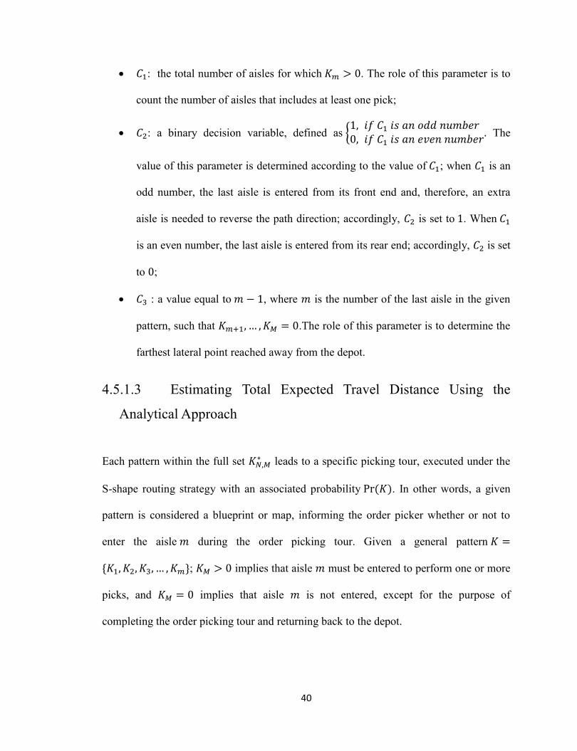
40
𝐶 : the total number of aisles for which . The role of this parameter is to
count the number of aisles that includes at least one pick;
𝐶 : a binary decision variable, defined as { 𝑓 𝐶 𝑠 𝑎 𝑢 𝑒𝑟 𝑓 𝐶 𝑠 𝑎 𝑒 𝑒 𝑢 𝑒𝑟
The
value of this parameter is determined according to the value of 𝐶 ; when 𝐶 is an
odd number, the last aisle is entered from its front end and, therefore, an extra
aisle is needed to reverse the path direction; accordingly, 𝐶 is set to . When 𝐶
is an even number, the last aisle is entered from its rear end; accordingly, 𝐶 is set
to ;
𝐶 : a value equal to , where is the number of the last aisle in the given
pattern, such that .The role of this parameter is to determine the
farthest lateral point reached away from the depot.
4.5.1.3 Estimating Total Expected Travel Distance Using the
Analytical Approach
Each pattern within the full set leads to a specific picking tour, executed under the
S-shape routing strategy with an associated probability ( ). In other words, a given
pattern is considered a blueprint or map, informing the order picker whether or not to
enter the aisle during the order picking tour. Given a general pattern
{ }; implies that aisle must be entered to perform one or more
picks, and implies that aisle is not entered, except for the purpose of
completing the order picking tour and returning back to the depot.

41
Therefore, the total expected travel distance required to complete a pick list of size in
a warehouse with aisles is obtained from the summation of the expected pattern-based
travel distances for every pattern in the fully enumerated set , where the expected
pattern-based travel distance of a pattern is obtained by multiplying the probability of a
pattern (Equation 4.8) by its travel distance (Equation 4.10). This gives:
( ) ∑ ( ) × (K)
𝐾 ∈ 𝐾𝑁 𝑀
4.11
where:
( ): the total expected travel distance for a given pair ( , ) using the
analytical approach;
( ): the pattern-based travel distance;
( ): the probability of pattern to occur.
4.5.2 Monte Carlo Simulation Approach
In this section, the Monte Carlo simulation approach is presented through four main
aspects; the need of the simulation approach due to the limitations of the analytical
approach, the concept of generating random patterns, the estimation of the total expected
travel distance using the simulation approach, and finally the validation of the Monte
Carlo simulation approach.

42
4.5.2.1 Limitations of Analytical approach
The analytical approach is theoretically designed to investigate all patterns obtained from
any given pair of and , regardless of the size of the fully enumerated set .
However, due to practical computational limitations, the analytical approach requires a
very long processing time to evaluate excessively large or even moderate sizes of .
The use of large and values makes the analytical approach impractical due to the
excessively large sets of patterns that result.
Table 2 presents the size of the fully enumerated sets for pick lists of size
and , along with different warehouse layouts of and . It is
clear from the table that a rapid increase in the size of occurs as M and/or N
increase, due to the exponential-factorial effect. Even with the moderate case of a pick
list of picks and a warehouse with main storage aisles, there are over
× possible patterns to be evaluated. Therefore, the analytical approach is
practically limited to investigating and values producing reasonably- and
practically-sized fully enumerated sets, which may be around million patterns.

43
Table 2: Size of 𝑲𝑵 𝑴
for Various N and M
Pick list size
Number of Storage Aisles
𝑴 𝟏𝟎 𝑴 𝟐𝟎 𝑴 𝟑𝟎
𝑵 𝟔 × × ×
𝑵 𝟏𝟐 × × ×
𝑵 𝟑𝟎 × 0 8 × 0 8 ×
𝑵 𝟓𝟎 × 0 8 × 8 8 ×
4.5.2.2 Generating Random Patterns
A Monte Carlo simulation approach is developed to overcome the limitations of the
analytical approach. The idea behind this simulation approach is to substitute the role of
the pattern generator with a process which randomly generates a predetermined number
of runs , where each run represents a random pattern. This random set of runs is
determined, instead of generating the fully enumerated set for a given , and that
may consist of billions of patterns.

44
For the purpose of generating random patterns, the following function and variables are
defined:
Cumulative distribution function of the probability mass function ( ):
𝑃 ( )
{
∑ ( )
=
≤
𝑂𝑡ℎ𝑒𝑟𝑤 𝑠𝑒
4.12
: the total number of random patterns (runs);
𝑟 : a random number associated with pick among picks.
The process of generating a random pattern based on a given pick list of size , and a
warehouse with aisles, starts with assigning a random number, 𝑟 , between and , to
each of the picks. Next, an aisle is selected to contain each of these picks, by finding
the first aisle among the aisles that happens to have a cumulative value of ( ) at
least equal to the random value 𝑟 associated with the pick 𝑃 ( ) 𝑟 . This process is
repeated until the runs are generated. The flow chart in Figure 11 below shows the
steps in the process of generating random patterns.

45
Start
Enter the pick list size (N)
Enter the total number of storage aisles (M)
Enter the number of random runs (R)
Pick number (n) =1
Aisle number (m)=1
n ≤ N Yes
Run number(Rn) ≤ Total Number of runs (R)
Yes
End
No
Generate random number (rn)
m ≤ M
Random number(rn)≤ PM(m)
Yes
Pick number (n)in aisle number(m)
No
Locate pick number (n) in aisle number (m)
Increment pick number (n) by 1
Yes
Increment aislenumber (m) by 1
No
Run number (Rn)=1
Increment run number (Rn) by 1
No
Figure 11: Flow chart for generating R random patterns using Monte Carlo simulation approach

46
A randomly generated set for a given pair of and containing patterns is denoted
by . Each pattern is defined as follows:
{ } 4.13
such that ∑
=
4.14
where : the number of picks present in aisle .
For an example of how a random pattern might be generated, assume that after assigning
a given group of items into a warehouse with , the obtained discrete probabilities
of a single pick are ( ) , ( ) , and ( ) . The cumulative
distribution would be 𝑃 ( ) , 𝑃 ( ) , and 𝑃 ( ) . We are interested in
generating a random pattern for a pick list of 3 picks in that warehouse, given that the
randomly generated numbers 𝑟 , 𝑟 , and 𝑟 8 are associated with the
first, second, and the third picks, respectively. The first pick would be located in the first
aisle, as (𝑃 ( ) ) (𝑟 ). Similarly, the second pick would be located in the
first aisle, as (𝑃 ( ) ) (𝑟 ). The third pick would be located in the third
aisle, as (𝑃 ( ) ) (𝑟 8 ). The resultant random pattern would be defined
as { }.

47
4.5.2.3 Estimating Total Expected Travel Distance Using
Simulation
After generating a random set , the expected total travel distance required to
complete a pick list of size from a warehouse with aisles is obtained by averaging
the summation of the travel distances of every random pattern in , using the
following function:
(
) ∑ ( )𝐾𝑆 ∈ 𝐾𝑆𝑁 𝑀
𝑅
4.15
where:
( ): the total expected travel distance for a given pair ( , ) using the
simulation approach;
( ): the travel distance corresponding to pattern , obtained by the pattern-
based travel distance function given in Equation 4.10.
4.5.2.4 Validation of Monte Carlo Simulation Approach
The set always has a large number of randomly generated patterns . According
to the central limit theorem, a hypothesis test is conducted to validate the Monte Carlo
simulation approach.
The analytical approach is utilized to validate the simulation approach by executing a
two-sided hypothesis test at a 99 percent confidence level for the expected total travel

48
distance values for given pairs of , and , obtained by both approaches. The test is
described as follows:
Hypotheses on the expected total travel distance:
H0 ( ) (
)
H ( ) ≠ (
)
4.16
Test statistic:
0
( ) (
)
𝐸( 𝑆𝑁 𝑀𝑅 )/√ 4.17
where 𝐸( 𝑆𝑁 𝑀𝑅 ) √∑ ( ( ) (
)) 𝐾𝑆 ∈ 𝐾𝑆𝑁 𝑀𝑅
4.18
𝐸( 𝑆𝑁 𝑀𝑅 ) is an estimate of the standard deviation of ( ) values, implied by the
random patterns in for a given pair of and .
Decision criterion for rejecting the null hypothesis:
𝑃- 𝑎𝑙𝑢𝑒( 0) 4.19

49
Chapter 5
Implementation
In this chapter, 600 items and six feasible layout alternatives have been chosen for
implementing the methodology, and for performing the desired numerical analysis in
such a way that the combined effects of the three storage assignment policies and the
warehouse shape on the efficiency of order picking in terms of the travel distance, as well
as the performance of each of the three storage polices under consideration, can be
thoroughly analyzed.
5.1 Items
The developed methodology is implemented by considering a group of 600 items with
items per unit time and storage locations. A sample of these
items along with their attributes is presented in Table 3.
Table 3: Sample of Items Data
Item No. 𝑫𝒊 𝑺𝒊 𝑫𝑺𝑹𝒊 𝑹𝒊
1 3357 2 1678.5 0.952524
2 2136 2 1068 0.560937
3 3164 1 3164 0.658153
4 843 2 421.5 0.179097
5 1463 4 365.75 0.321327
6 1504 4 376 0.210995
7 3503 5 700.6 0.692759
8 3552 4 888 0.977731
9 1683 3 561 0.206321
10 3684 5 736.8 0.24869

50
5.2 Warehouse Layout Alternatives
Six different feasible warehouse layout structure alternatives represented by
{( ) ( ) ( ) ( 8 )
( 8) ( 8)} are selected to be investigated with the
three storage assignment policies. All six layout structures share the same dimensional
parameters of m, 8 m, and 8 m. A scaled layout representation
showing the dimensional differences between the six warehouse layout alternatives is
depicted in Figure 12.
Figure 12: A scaled layout representation of the six layout alternatives in D*

51
5.3 Python Code
The software code for this thesis is developed in the Python language, in order to
facilitate efficient implementation, and to obtain full sets of results for a wide range of
scenarios and situations. The Python code is presented in its entirety in Appendix B. The
code is explained in the following six sections.
5.3.1 Input Parameters and Item’s Data
The Python code starts with the function enter_params, which is used to allow the user
to specify the layout and dimensional parameters of the warehouse including , , ,
, and . Also, this function allows the user to enter the maximum size of the pick
list to be investigated using both the analytical approach and the Monte Carlo
simulation approach, in addition to the number of random runs, , to be provided by the
simulation approach. The function interactive is used at this stage to extract the items
and their attributes from the sample_data.csv file, and then it generates multiple data
sets, one for each assignment storage policy.
5.3.2 Item Allocation
After getting all necessary parameters, variables, and extracting all items and their
attributes, Aisle and Item classes are used to track and control both the items and the
aisles during the execution of the item allocation within the warehouse using any of the
three assignment storage policies. The Aisle class is used to control and track the position
and the number of assigned items within the aisles indicated by the number of storage

52
locations in which each assigned item is located. Also, the Aisle class is used to track and
update the current capacity of each side of every main storage aisle in the layout. The
Item class is used to keep track of individual item attributes including the name, the
demand, the storage requirements, and its location within the warehouse. Also, the Item
class is used to facilitate the sorting of the items, as required by the storage assignment
policies. The function Layout in cooperation with the Aisle class are used to create a
series of double-sided storage aisles with a number of storage locations in them, based on
the parameters and provided by the function enter_param, which is called from the
assign function and does not need to be called from the user’s code. The function
expected_values, in cooperation with the Item class, is used to sort a given group of
items according to the specific criteria of one of the three assignment storage policies.
Based on the classes, Aisle and Item, and in addition to the functions Layout and
expected_values, the function Assign is used to assign the items within a given
warehouse layout, and to return the probability values ( ). The function Assign
includes four sub-functions: one for each of the assignment storage polices. The four
functions are named assign_FullTurnOverNN, assign_FullTurnOverNS,
assign_NearestLocation, and assign_Random, which only differ in the final sorting of
the given items provided by the function expected_values.
5.3.3 Travel Distance Estimation Using the Analytical Approach
The function possibilities is used to generate the fully enumerated set of all possible
patterns , along with the probabilities ( ) associated with the generated pattern,
based on the given values of , , and the values of ( ) provided by the function
Assign for each of the three assignment storage policies.

53
The function distance is used to calculate the pattern-based travel distance for every
pattern in the fully enumerated set obtained by the function possibilities. This function is
represented in Equation 4.10, and takes into account the values , , , and . The
function total_distance is used to calculate the total expected travel distance for a given
pair of N and M based on the distances provided by the function distance, and the
probabilities ( ) provided by the function possibilities. The function total_distance is
represented in Equation 4.11.
5.3.4 Travel Distance Estimation Using the Simulation Approach
The function Monte_carlo is used to perform a series of a predetermined number of
random runs, . The outcome of every single run represents a random pattern. Then,
using the function distance, the pattern-based travel distance associated with each of the
random patterns is obtained. The function Monte_carlo is used to calculate the total
expected travel distance by averaging all the distances obtained the function distance.
5.3.4.1 Validation of the Simulation Approach
The function confidence is used to validate the Monte Carlo simulation approach based
on the values obtained by the analytical approach. This function is responsible for
obtaining the mean and standard deviation for a given number of runs, and then
performing a two-sided hypothesis test at a specific confidence level; it returns the test’s
associated P-values.

54
5.3.5 Outcomes and Results
Finally, all of the obtained outcomes for each of the assignment storage policies are
provided using the function interactive in form of csv files. The outcomes include the
locations of the assigned items within the warehouse, the ( ) values, the analytical
results, and the simulation results along with their validation results.
5.3.6 Computational Time
The CPU times (seconds) on a 2.5Ghz Intel i5 processor with 6GB RAM required for
estimating the total expected travel distances under each of the three assignment storage
policies using either the analytical or the simulation approach for selected values of
and are presented in Table 4.
Table 4: Sample of CPU Times (seconds) for selected pairs of N, and M
Analytical Simulation
N 𝑴 𝟏𝟓,𝑩 𝟔𝟎 𝑴 𝟑𝟎,𝑩 𝟑𝟏 𝑴 𝟏𝟓,𝑩 𝟔𝟎 𝑴 𝟑𝟎,𝑩 𝟑𝟏
1 <1.00 <1.00 <1.00 <1.00
2 <1.00 <1.00 <1.00 <1.00
3 <1.00 1.21 <1.00 <1.00
4 1.311 39.88 <1.00 10.41
5 21.60 1300.56 8.72 11.58
6 365.82 - 9.73 12.77
7 5487.35 - 11.91 16.17
8 - - 12.91 17.41
20 - - 25.39 34.36
50 - - 54.74 76.33
90 - - 81.37 126.69

55
5.4 Item Allocation
The same 600 items are allocated into each warehouse layout alternative in the set by
implementing all three storage assignment policies, for the purpose of estimating the
probability of a single pick’s presence in aisle m, represented as ( ). The values of
the probability mass function ( ) obtained under the full-turnover policies, including
its two distinct assignment directions, north-north and north-south; nearest-location; and
random storage assignment policies for every aisle in each layout alternative in are
presented in Figure 13.

56
Fifth Layout(M5 =6,B5 =148)
Aisle m
0 1 2 3 4 5 6 7
Pro
bab
ility
of
a Si
ngl
e P
ick
in A
isle
m
0.0
0.1
0.2
0.3
0.4
0.5
Initial Layout(M1 =30,B1 =31)
Aisle m0 5 10 15 20 25 30 35
Pro
bab
ility
of
a Si
ngl
e P
ick
in A
isle
m
0.00
0.02
0.04
0.06
0.08
0.10
0.12
0.14
Second Layout(M2 =15,B2 =60)
Aisle m
0 2 4 6 8 10 12 14 16
Pro
bab
ility
of
a Si
ngl
e P
ick
in A
isle
m
0.00
0.05
0.10
0.15
0.20
0.25
Third Layout(M3 =10,B3 =90)
Aisle m
0 2 4 6 8 10 12
Pro
bab
ility
of
a Si
ngl
e P
ick
in A
isle
m
0.00
0.05
0.10
0.15
0.20
0.25
0.30
Fourth Layout(M4 =8,B4 =112)
Aisle m
0 2 4 6 8 10
Pro
bab
ility
of
a Si
ngl
e P
ick
in A
isle
m
0.00
0.05
0.10
0.15
0.20
0.25
0.30
0.35
Final Layout(Mf =5,Bf =178)
Aisle m0 1 2 3 4 5 6
Pro
bab
ility
of
a Si
ngl
e P
ick
in A
isle
m
0.0
0.1
0.2
0.3
0.4
0.5
Full-turnover (NS,NN)Random Nearest Location
Full-turnover (NS,NN)Random Nearest Location
Full-turnover (NS,NN)Random Nearest Location
Full-turnover (NS,NN)Random Nearest Location
Full-turnover (NS,NN)Random Nearest Location
Full-turnover (NS,NN)Random Nearest Location
Figure 13 indicates that the full-turnover storage assignment policy results in a declining
trend of ( ) values, such that ( ) is the largest and ( ) is the smallest, which
implies that, under the full-turnover policy, the probability of finding a single pick is
highest in the first aisle and decreases aisle by aisle. This is explained by the manner in
which the full-turnover policy sorts the items according to their demand to size ratio;
Figure 13: 𝐩𝐌(𝐦) values of the three storage policies for the six layouts

57
. Accordingly, the aisles closest to the depot usually contain the items with the
highest demand. Also, it is important to mention that both north-north and north-south
assignment directions of the full-turnover policy produce exact ( ) values. This
happens because the items allocated in each main storage aisle will be same for north-
north and north-south assignment directions, although their storage locations within the
main aisle will be different.
The nearest-location storage assignment policy results in ( ) values which exhibit
cyclic, peak-valley behavior along the aisles. The reason for this behavior is because
the nearest-product policy incrementally sorts the items according to their storage
requirements; . In other words, items are split into multiple groups based on , so the
items in each group share the same , and then the items in each group are sorted
according to their demand. Therefore, each of the sorted groups features a peak ( )
value caused by the items with the highest demand in the group, followed by a valley
( ) value caused by the item with lowest demand.
The random storage assignment policy results in almost leveled ( ) values among the
warehouse’s aisles. This is explained by the random manner in which all items are
allocated into the aisles with no preference of one over another, regardless of their
demand and storage requirements.
The data in Figure 13 suggests that ( ) values obtained by the nearest-location
policy approach the ones obtained by the full-turnover policy as the number of storage
aisles decreases and the number of storage locations in each of these aisles increases
simultaneously. In other words, the impact of the nearest-location policy approaches the

58
impact of full-turnover as the density of the allocated items per storage aisle significantly
increases. The ( ) values obtained by the random storage policy get more balanced
as the density of picks significantly increases in .
5.5 Validation of the Monte Carlo Simulation Approach
The Monte Carlo simulation approach is validated against the analytical approach. Two-
sided hypothesis tests are performed to determine whether or not the total expected travel
distance, ( ), and (
) values obtained by both approaches, are similar at a
percent confidence level. Therefore, limited and practical ranges of values among
all six warehouse layout alternatives in are considered to obtain the ( ), and
( ) values.
The results of the simulation approach validation based on the total expected travel
distance values required to complete pick lists of sizes from the final
layout in with , and 8 are presented in Table 5. The results clearly
suggest a conclusion that the values of both approaches are similar at a percent
confidence level, as all p-values are larger than the significance level of percent.
Also, the test indicates that the maximum absolute difference between the values
resulting from the two approaches does not exceed .

59
Table 5: Validation Results Based on Final Layout, 𝑴𝒇 = 5 and 𝑩𝒇 = 178
N
Full-turnover (NN & NS) The Nearest-location Random
Analytical
Sim
ulated
|Difference%|
P
Analytical
Sim
ulated
|Difference%|
P
Analytical
Sim
ulated
|Difference%|
P
1
341.845 341.843 0.00043 0.86 348.731 348.731 0.00012 0.96 362.281 362.278 0.00077 0.78
2
355.585 355.603 0.00526 0.03 365.125 365.130 0.00143 0.57 379.886 379.886 0.00003 0.99
3
461.689 461.701 0.00261 0.80 495.775 495.728 0.00945 0.35 530.609 530.582 0.00517 0.58
4
539.268 539.279 0.00199 0.83 581.854 581.824 0.00514 0.54 621.011 620.950 0.00974 0.15
5
592.559 592.547 0.00203 0.80 637.400 637.401 0.00009 0.99 675.515 675.571 0.00824 0.12
6
630.670 630.581 0.01416 0.04 678.220 678.156 0.00947 0.12 717.552 717.483 0.00955 0.07
7
659.518 659.500 0.00276 0.66 711.671 711.707 0.00512 0.39 755.703 755.658 0.00603 0.28
8
682.616 682.594 0.00319 0.59 741.245 741.223 0.00293 0.62 791.498 791.502 0.00051 0.93
9
702.035 702.057 0.00315 0.59 768.012 767.930 0.01061 0.08 824.409 824.412 0.00027 0.96
10
719.002 719.047 0.00622 0.29 792.333 792.290 0.00537 0.38 853.773 853.763 0.00117 0.83
11
734.247 734.226 0.00284 0.63 814.449 814.489 0.00493 0.41 879.286 879.302 0.00172 0.75
In similar manner, the simulation approach is validated based on the other five feasible
layout alternatives in . The validation results, obtained for each of the five layout
alternatives, show that both approaches provide similar values at a 99 percent confidence
level. The complete analysis of the five feasible layouts is presented in Appendix A.

60
5.6 Analysis of the Estimated Total Expected Travel Distance
The Monte Carlo simulation approach is utilized to estimate the total expected travel
distance ( ) required to pick all items on pick lists of sizes from
each set of layout parameters and in , with the assumption that the S-shape
routing policy is to be used.
5.6.1 Effects of Storage Assignment Policies and Pick list Size
The total expected travel distances versus the pick list size under each of the full-turnover
policies, including the north-north and north-south assignment directions; nearest-
location; and random storage policies for the layouts ( ), (
), ( ), ( 8 ), ( 8), and
( 8) are presented in Figure 14.

61
Initial Layout(M1 =30,B1 =31)
Pick List Size(N)
0 20 40 60 80 100
Tota
l Exp
ecat
ed T
rave
l Dis
tan
ce(m
)
0
150
300
450
600
750
900
1050
1200
1350
1500
Second Layout(M2 =15,B2 =60)
Pick List Size(N)
0 20 40 60 80 100
Tota
l Exp
ecat
ed T
rave
l Dis
tan
ce(m
)
0
150
300
450
600
750
900
1050
1200
1350
1500
Third Layout(M3 =10,B3 =90)
Pick List Size(N)
0 20 40 60 80 100
Tota
l Exp
ecat
ed T
rave
l Dis
tan
ce(m
)
0
150
300
450
600
750
900
1050
1200
1350
1500
Fourth Layout(M4 =8,B4 =112)
Pick List Size(N)
0 20 40 60 80 100
Tota
l Exp
ecat
ed T
rave
l Dis
tan
ce(m
)
0
150
300
450
600
750
900
1050
1200
1350
1500
Fifth Layout(M5 =6,B5 =148)
Pick List Size(N)
0 20 40 60 80 100
Tota
l Exp
ecat
ed T
rave
l Dis
tan
ce(m
)
0
150
300
450
600
750
900
1050
1200
1350
1500
Final Layout(Mf =5,Bf =178)
Pick List Size(N)
0 20 40 60 80 100
Tota
l Exp
ecat
ed T
rave
l Dis
tan
ce(m
)
0
150
300
450
600
750
900
1050
1200
1350
1500
Full-turnover (NN,NS)
Random
Nearest Location
Full-turnover (NN,NS)
Random
Nearest Location
Full-turnover (NN,NS)
Random
Nearest Location
Full-turnover (NN,NS)
Random
Nearest Location
Full-turnover (NN,NS)
Random
Nearest Location
Full-turnover (NN,NS)
Random
Nearest Location
By comparing the total expected travel distance values from all six layouts using the
three different policies, as illustrated in Figure 14, the effects of the three storage
assignment policies can be determined. The full-turnover policy, in which its two distinct
assignment directions, north-north and north-south, have similar outcomes, results in the
lowest total expected travel distances. This is due to the declining trend of the ( )
Figure 14: 𝐄(𝐃𝐒𝐍 𝐌𝐑 ) values of the three storage policies for the six layouts

62
values obtained by the full-turnover policy. In other words, the order picker is more
likely to enter the first few aisles, which are the closest to the depot and have the highest
( ) values, rather than entering all aisles, including other aisles with lower ( )
values, to retrieve the picks.
The nearest-location policy results in moderate total expected travel distances, compared
to the full-turnover and the random policies. This is caused by the cyclic behavior of
( ) values among the aisles, which means that the order picker is more likely to
enter aisles with a peak ( ) value than the other aisles, including aisles with
valley ( ) values, to retrieve the picks. Also, in this case, the number of aisles to
be entered is always higher than those in the full-turnover policy, which is why the full-
turnover policy generally results in shorter total expected travel distances than the
nearest-product policy.
The random storage policy results in the largest total expected travel distances among the
three storage policies. This is due to relatively even ( ) values, meaning an order
picker is likely to enter more of the aisles to retrieve the picks, when compared to
the previous storage policies.
The results also clearly indicate that the total expected travel distance values obtained by
a policy generally approach the values of the other policies as the size of the pick list
increases. A larger pick list size results in a higher density of picks per storage aisle,
which eventually necessitates the order picker to enter most of the aisles, regardless of
the storage policy applied.

63
5.6.2 Effect of Warehouse Shape
For the purpose of magnifying and maintaining the effect of the warehouse’s shape, the
pick list size of range is divided into eight ranges of picks: ,
, , , , ,
,and .
The ( )̅̅ ̅̅ ̅̅ ̅̅ ̅̅ ̅̅ ̅ values obtained for each of the eight ranges under the three storage
assignment policies for each of the six feasible warehouse layout alternatives in are
presented in Figure 15.

64
N1=2,...,5
Layout Alternatives in D*
M1=30,B1=31 M2=15,B2=60 M3=10,B3=90 M4=8,B4=112 M5=6,B4=148 Mf=5,Bf=178
Eq
ua
lly A
vera
ged
To
tal E
xpe
cte
d T
rave
l Dis
tan
ce
350
400
450
500
550
600
650Full-turnover(NN,NS)
Random
Nearest Location
N2=6,...,10
Layout Alternatives in D*M1=30,B1=31 M2=15,B2=60 M3=10,B3=90 M4=8,B4=112 M5=6,B4=148 Mf=5,Bf=178
Eq
ua
lly A
vera
ged
To
tal E
xpe
cte
d
Tra
vel D
ista
nce
550
600
650
700
750
800
850
Full-turnover(NN,NS)
Random
Nearest Location
N3=11,...,15
Layout Alternatives in D*
M1=30,B1=31 M2=15,B2=60 M3=10,B3=90 M4=8,B4=112 M5=6,B4=148 Mf=5,Bf=178
Eq
ua
lly A
vera
ged
To
tal E
xpe
cte
d T
rave
l Dis
tan
ce
650
700
750
800
850
900
950Full-turnover(NN,NS)
Random
Nearest Location
N4=16,...,20
Layout Alternatives in D*
M1=30,B1=31 M2=15,B2=60 M3=10,B3=90 M4=8,B4=112 M5=6,B4=148 Mf=5,Bf=178
Eq
ua
lly A
vera
ged
To
tal E
xpe
cte
d T
rave
l Dis
tan
ce
750
800
850
900
950
1000
1050
Full-turnover(NN,NS)
Random
Nearest Location
N5=21,...,25
Layout Alternatives in D*M1=30,B1=31 M2=15,B2=60 M3=10,B3=90 M4=8,B4=112 M5=6,B4=148 Mf=5,Bf=178
Eq
ua
lly A
vera
ged
To
tal E
xpe
cte
d
Tra
vel D
ista
nce
800
850
900
950
1000
1050
1100
1150N6=26,...,35
Layout Alternatives in D*M1=30,B1=31 M2=15,B2=60 M3=10,B3=90 M4=8,B4=112 M5=6,B4=148 Mf=5,Bf=178
Eq
ua
lly A
vera
ged
To
tal E
xpe
cte
d T
rave
l Dis
tan
ce
800
900
1000
1100
1200
1300
Full-turnover(NN,NS)
Random
Nearest Location
Full-turnover(NN,NS)
Random
Nearest Location
N7=36,...,45
Layout Alternatives in D*M1=30,B1=31 M2=15,B2=60 M3=10,B3=90 M4=8,B4=112 M5=6,B4=148 Mf=5,Bf=178
Eq
ua
lly A
vera
ged
To
tal E
xpe
cte
d
Tra
vel D
ista
nce
800
900
1000
1100
1200
1300
1400N8=46,...,90
Layout Alternatives in D*M1=30,B1=31 M2=15,B2=60 M3=10,B3=90 M4=8,B4=112 M5=6,B4=148 Mf=5,Bf=178
Eq
ua
lly A
vera
ged
To
tal E
xpe
cte
d T
rave
l Dis
tan
ce
800
900
1000
1100
1200
1300
1400
1500
Full-turnover(NN,NS)
Random
Nearest Location
Full-turnover(NN,NS)
Random
Nearest Location
Figure 15: 𝐄(𝐃𝐒𝐍 𝐌𝐑 )̅̅ ̅̅ ̅̅ ̅̅ ̅̅ ̅̅ values of the three storage policies for the eight ranges of N

65
Figure 15 illustrates the fact that the ( )̅̅ ̅̅ ̅̅ ̅̅ ̅̅ ̅̅ ̅ values for the eight ranges of under
each of the three storage policies exhibit a concave up behavior over the six feasible
layouts in , in sequence from the initial layout to the final layout.
For instance, the pick list size ranges, , , and
, can be used to explain how the variations in the warehouse shape result in the
concave up behavior of the ( )̅̅ ̅̅ ̅̅ ̅̅ ̅̅ ̅̅ ̅ values. A comparison of the graphs in Figure 15
indicates that the averaged total expected travel distance gradually decreases over the
initial, second, third, fourth and fifth layouts. This decrease is caused by the reduction in
the number of storage aisles in each of the five layouts the order picker may have
traversed to complete a given number of picks. Although this reduction is coupled with a
simultaneous increase in the number of storage locations in each of these aisles, resulting
in an extension of the length of each aisle, in the case of these five layout alternatives, the
reduction in travel distance due to decreasing the number of aisles overcomes the
simultaneous increase in travel distance due to extending the length of the vertical aisles,
eventually leading to an overall reduction in the averaged total expected travel distance.
The described reduction behaviour no longer occurs in the final layout alternative. This is
because the reduction in the travel distance due to reducing the number of total storage
aisles is no longer sufficient to overcome the increase in travel distance caused by
increasing the depth of the aisles. The result is a rapid increase in the averaged total
expected travel distance. For the exact same reasons, the concave up behavior is repeated
for the ranges , , , , and
, in which the reduction behavior no longer occurs after the second and the third
layouts for , , , and , , respectively.

66
Figure 15 also indicates that, under the full-turnover storage policy, the second layout
alternative with achieves the local minimum averaged total expected
travel distances of m, 8 m and m, for the pick list sizes of ranges
, , and , respectively; the third layout alternative with
achieves the local minimum averaged total expected travel distances
of m, and 8 m for the pick list sizes of ranges, , and
, respectively; and the fifth layout alternative with 8 achieves
the local minimum averaged total expected travel distances of 8 m, 8 m, and 8 m
for the pick list sizes of ranges , , and ,
respectively.

67
N1=2,...,5
M1=30,B1=31 M2=15,B2=60 M3=10,B3=90 M4=8,B4=112 M5=6,B4=148 Mf=5,Bf=178
Per
form
ance
dif
fere
nce
s %
0
5
10
15
20
25
30N2=6,...,10
M1=30,B1=31 M2=15,B2=60 M3=10,B3=90 M4=8,B4=112 M5=6,B4=148 Mf=5,Bf=178
Per
form
ance
dif
fere
nce
s %
0
5
10
15
20
25
30
N3=11,...,15
M1=30,B1=31 M2=15,B2=60 M3=10,B3=90 M4=8,B4=112 M5=6,B4=148 Mf=5,Bf=178
Per
form
ance
dif
fere
nce
s %
0
5
10
15
20
25
30N4=16,...,20
M1=30,B1=31 M2=15,B2=60 M3=10,B3=90 M4=8,B4=112 M5=6,B4=148 Mf=5,Bf=178
Per
form
ance
dif
fere
nce
s %
0
5
10
15
20
25
30
N5=21,...,25
M1=30,B1=31 M2=15,B2=60 M3=10,B3=90 M4=8,B4=112 M5=6,B4=148 Mf=5,Bf=178
Per
form
ance
dif
fere
nce
s %
0
5
10
15
20
25
30N6=26,...,35
M1=30,B1=31 M2=15,B2=60 M3=10,B3=90 M4=8,B4=112 M5=6,B4=148 Mf=5,Bf=178
Per
form
ance
dif
fere
nce
s %
0
5
10
15
20
25
30
N8=46,...,90
M1=30,B1=31 M2=15,B2=60 M3=10,B3=90 M4=8,B4=112 M5=6,B4=148 Mf=5,Bf=178
Per
form
ance
dif
fere
nce
s %
0
5
10
15
20
25
30N7=36,...,45
M1=30,B1=31 M2=15,B2=60 M3=10,B3=90 M4=8,B4=112 M5=6,B4=148 Mf=5,Bf=178
Per
form
ance
dif
fere
nce
s %
0
5
10
15
20
25
30
Full-turnover(NN &NS),Random Full-turnover(NN &NS),Nearest-locationNearest-location,Random
Full-turnover(NN &NS),Random Full-turnover(NN &NS),Nearest-locationNearest-location,Random
Full-turnover(NN &NS),Random Full-turnover(NN &NS),Nearest-locationNearest-location,Random
Full-turnover(NN &NS),Random Full-turnover(NN &NS),Nearest-locationNearest-location,Random
Full-turnover(NN &NS),Random Full-turnover(NN &NS),Nearest-locationNearest-location,Random
Full-turnover(NN &NS),Random Full-turnover(NN &NS),Nearest-locationNearest-location,Random
Full-turnover(NN &NS),Random Full-turnover(NN &NS),Nearest-locationNearest-location,Random
Full-turnover(NN &NS),Random Full-turnover(NN &NS),Nearest-locationNearest-location,Random
5.6.3 Performance Differences of the Storage Assignment Policies
The percentage differences in the performances of the three policies for the eight pick list
size ranges in the six warehouse layout alternatives are presented in Figure 16.
Figure 16: Percentage difference in performance of the three storage policies

68
Based on Figure 16, it can be seen that the difference in performance between the three
storage assignment policies decreases gradually over the eight pick list size ranges,
beginning with , and ending with , and this is explained by
the fact that the density of picks per aisle m increases as the pick list size increases. This
means that the order picker will enter more aisles to perform the required picks,
regardless of the storage assignment policy applied in allocating the items. The largest
difference in performance between the full-turnover and the random storage policies
starts at about with , and ends at about with ;
the largest difference in performance between the full-turnover and the nearest-location
policies starts at about with , and ends at about with
; and the largest difference in performance between the nearest-location and the
random storage policies starts at about with , and ends at about
with . The smallest difference in performance between the full-turnover
and the random storage policies starts at about 8 with , and ends at
about with the smallest difference in performance between the
full-turnover and the nearest-location policies starts at about with , and
ends at about with ; and the smallest difference in performance
between the nearest-location and the random storage policies starts at about 8 with
, and ends at about with .

69
5.7 Special Case: Pick List Sizes Follow an Exponential
Distribution
In the case when all pick list sizes of the range are equally weighted, this
means that the ( ) values are identical for all pick list sizes. Therefore, ( ) is
defined according to a discrete uniform probability distribution defined as follows:
( ) {
8 ≤ ≤
𝑂𝑡ℎ𝑒𝑟𝑤 𝑠𝑒 5.1
In some practical real-life situations, it might happen that the pick list sizes are
exponentially distributed with a given mean, , which means that the relative weights of
the pick lists of sizes are no longer identical. In fact, in this case, the
relative weights of every pick list of size N are determined by an exponential probability
density function. Therefore, ( ) is defined as follows:
( ) {
𝑒− 𝛽 ≤
𝑂𝑡ℎ𝑒𝑟𝑤 𝑠𝑒
5.2

70
Accordingly, the averaged values of the total expected travel distances, ( )̅̅ ̅̅ ̅̅ ̅̅ ̅̅ ̅̅ ̅,
obtained for each of the three storage assignment policies for pick lists of sizes
are calculated as follows:
( )̅̅ ̅̅ ̅̅ ̅̅ ̅̅ ̅̅ ̅ ∑ (
) × ( )
=90
=
5.3
where:
( ): the total expected travel distance required to pick all items from a pick
list of size in a warehouse layout with aisles, obtained through the use of the
Monte Carlo simulation approach;
( ): probability that the pick list has a particular size , which is chosen to be
either equally weighted or exponentially distributed according to the functions
given in Equations 5.1 and 5.2, respectively.
Represented in Figure 17 are two cases in which the pick list sizes are exponentially
distributed; the first case assumes a mean pick list size of picks (i.e., ), while
the second case assumes a mean of picks (i.e., ). These two cases are graphed
with equally distributed pick list sizes, relative to the probability of for the full range
of pick list sizes.

71
Pick-list Size N
0 20 40 60 80 100
Pro
bab
ility
of
N
0.00
0.01
0.02
0.03
0.04
0.05
0.06
0.07
Uniform
Exp,Beta=15
Exp,Beta=30
Considering the fifth layout in with 8, the averaged values of the
total expected travel distances, ( )̅̅ ̅̅ ̅̅ ̅̅ ̅̅ ̅̅ ̅, obtained under the three storage assignment
policies for completing a pick list of sizes , with ( ) values based on
exponential distributions with and , in addition to the equally weighted
( ) are presented in Figure 18.
Figure 17: Probability of pick-list of sizes 𝑵 𝟐 𝟗𝟎 based on exponential and uniform distributions

72
0.0
100.0
200.0
300.0
400.0
500.0
600.0
700.0
800.0
900.0
Full-turnover (NN &NS)
Nearest-location Random
62
0.4
65
2.3
67
8.6
68
0.1
70
5.6
72
3.9
82
2.5
83
8.5
84
7.3
Exp,β=15 Exp,β=30 Uniform
It is apparent from Figure 18 that the ( )̅̅ ̅̅ ̅̅ ̅̅ ̅̅ ̅̅ ̅ values are influenced by the relative
weight of the pick list sizes in a given warehouse. Accordingly, warehouse professionals
must pay attention to two primary aspects: the average size of the pick list, and the
manner in which the relative probabilities (i.e., weights) of pick list sizes are distributed.
(𝑫𝑺𝑵 𝑴𝑹 )̅̅ ̅̅ ̅̅ ̅̅ ̅̅ ̅̅ ̅̅ m
Figure 18: Averaged 𝐄(𝐃𝐒𝐍 𝐌𝐑 ) values of the three storage policies for the fifth layout based on exponential
and uniform distributions

73
Chapter 6
Conclusions and Further Research
We have presented a new methodology consisting of two primary approaches, the
analytical approach and the Monte Carlo simulation approach, for estimating the total
expected travel distance of a picking tour in a single-block, open-ended, picker-to-parts
warehouse. Through the use of these approaches, we evaluated the combined effects of
three storage assignment policies and the warehouse layout configuration, in terms of the
depth and the number of storage aisles. In doing so, we were able to determine the
optimal combination of the storage policy and the warehouse layout which achieves the
local minimum travel distance among all feasible combinations. Also, we compared the
performance of the full-turnover, the nearest-location and the random storage policies for
many warehouse layout configurations. This can be considered a contribution in the area
of improving the efficiency of order picking in picker-to-parts warehouses, and more
specifically, in implementing and evaluating the full-turnover storage assignment policy,
because the literature regarding the full-turnover storage policy in the context of order
picking travel distance is limited to the work performed by Caron et al. [2], [3], in which
he only compared the performance of the full-turnover policy to the performance of the
random storage policy in double-block, picker-to-parts warehouses. In addition, he
developed an analytical model for optimizing the number of storage aisles in double-
block warehouses, considering the full-turnover storage policy.

74
Our experimental evidence shows that the order picking travel distance is strongly
influenced by each item’s attributes, including their demand and storage requirements,
pick list size, warehouse layout in terms of the number and depth of its storage aisles, and
the storage policy used to allocate the items within the warehouse.
The results obtained from applying all three storage policies in various feasible
warehouse layout alternatives indicate that the full-turnover policy, including its two
assignment directions, the north-north and the north-south, always outperforms both the
nearest-location and the random storage policies, while the nearest-location policy
always outperforms the random policy. Accordingly, the random policy always results in
the highest order picking travel distances. Based on our experiments based on a group of
600 items allocated into six different feasible warehouse layout alternatives, we
concluded that the largest difference in performance between the full-turnover and
random storage policies is about , the largest difference in performance
between the nearest-product and random storage policies is about , and the
largest difference in performance between the nearest-location and random storage
policies is about .
We found that the layout shape significantly affects the order picking travel distance.
Under all three storage policies, a reduction in the travel distance occurred as a result of
decreasing the number of storage aisles the order picker may need to enter, until the
instance that the extra travel distance due to the corresponding extension in the depth of
the aisles, as needed to maintain the desired storage capacity of the warehouse, exceeded
the travel distance reduction due to lowering the number of storage aisles.
75
6.1 Directions for Further Research
Future research to extend this study could involve evaluating the impact of various
routing policies including the return, mid-point, and largest gap policies. Also, a future
study could compare the current three storage policies to other policies, including the
class-based and the volume-based storage assignment policies. Another important
extension to this study would be to evaluate the impact of adding one or more middle
cross aisles to the current layout structure on the order picking travel distance.

76
Bibliography
[1] Berglund, P., & Batta, R. (2012). Optimal placement of warehouse cross-aisles in a
picker-to-part warehouse with class-based storage. IIE Transactions, 44(2), 107-120.
[2] Caron, F., Marchet, G., & Perego, A. (1998). Routing policies and COI-based
storage policies in picker-to-part systems. International Journal of Production
Research, 36(3), 713-732.
[3] Caron, F., Marchet, G., & Perego, A. (2000). Optimal layout in low level picker-to-
part systems. International Journal of Production Research, 38(1), 101-117.
[4] Chan, F., & Chan, H. K. (2011). Improving the productivity of order picking of a
manual-pick and multi-level rack distribution warehouse through the
implementation of class-based storage. Expert Systems with Applications, 38, 2686-
2700.
[5] Coyle, J. J., Bardi, E. J., & Langley, C. J. (2003). The management of business
logistics: A supply chain perspective. (7th ed.). Mason,OH: South-Western College.
[6] De Koster, R., Le-Duc, T., & Roodbergen, K. J. (2007). Design and control of
warehouse order picking: A literature review. European Journal of Operational
Research, 182(2), 481-501.
[7] Den Berg, J. P. (1999). A literature survey on planning and control of warehousing
systems. IIE Transactions, 31(8), 751-762.
[8] Gu, J., Goetschalckx, M., & McGinnis, L. F. (2007). Research on warehouse
operation: A comprehensive review. European Journal of Operational Research,
177(1), 1-21.
[9] Hall, R. W. (1993). Distance approximation for routing manual pickers in a
warehouse. IIE Transactions, 25, 77-87.

77
[10] Heskett, J. L. (1963). Cube-per-order index – A key to warehouse stock location.
Transport and Distribution Management, 3, 27-31.
[11] Heskett, J. L. (1964). Putting the cube-per-order index to work in warehouse layout.
Transport and Distribution Management, 4, 23-30.
[12] Kallina, C., & Lynn, J. (1976). Application of the cube-per-order index rule for
stock location in distribution warehouse. Interfaces, 7(1), 37-46.
[13] Kubasad, S. R. (2010). Optimizing product placement for manual picking in
warehouses. (Unpublished Master of Engineering). Dalhousie University, Halifax,
Nova Scotia.
[14] Lambert, D. M., & Stock, J. R. (1998). In Ellram L. M. (Ed.), Fundamentals of
logistics management. Singapore: McGraw-Hill.
[15] Le-Duc, T., & De Koster, R. (2004). Travel distance estimation in single-block
ABC-storage strategy warehouses. In B. Fleiscmann, & A. Klose (Eds.),
Distribution logistics:Advanced solutions to practical problems. (pp. 184-200)
Springer.
[16] Le-Duc, T., & De Koster, R. (2005). Travel distance estimation and storage zone
optimization in a 2-block class-based storage strategy warehouse. International
Journal of Production Research, 43(17), 3561-3581.
[17] Petersen, C. G. (1997). An evaluation of order picking routing policies. .
International Journal of Operations & Production Management, 17(11), 1098-1111.
[18] Petersen, C. G. (2002). Considerations in order picking zone configuration.
International Journal of Operations & Production Management, 27(7), 793-805.
[19] Petersen, C. G., Aase, G., & Heiser, D. R. (2004). Improving order picking
performance through the implementation of class-based storage. International
Journal of Physical Distribution & Logistics Management, 34(7), 534-544.

78
[20] Roodbergen, K. J., & De Koster, R. (2001). Routing methods for warehouses with
multiple cross aisles. international journal of production research. International
Journal of Production Research, 39(9), 1865-1883.
[21] Roodbergen, K. J., Gunter, P. S., & Iris, F. A. V. (2008). Designing the layout
structure of manual order picking areas in warehouses. IIE Transactions, 40, 1032-
1045.
[22] Roodbergen, K. J., & Iris, F. A. V. (2006). A model for warehouse layout. IIE
Transactions, 38, 799-811.
[23] Tompkins, J. A., White, J. A., Bozer, Y. A., Frazelle, E. H., & Tanchoco, J. M. A.
(2003). Facilities planning. NJ: John Wiley & Sons.
[24] Vaughan, T. S., & Petersen, C. G. (1999). The effect of warehouse cross aisles on
order picking efficiency. International Journal of Production Research, 37(4), 881-
897.

79
Appendix A: Validation of Monte Carlo Simulation
The results of the simulation approach validation based on the initial layout of
, , and ; the second layout of , , and ;
the third layout of , , and ; the fourth layout of 8,
, and 8; and the fifth layout of , 8, and ;
are presented in Tables 6-10, respectively. The results clearly suggest the conclusion that
the values of both approaches are similar at a percent confidence level, as all p-values
are larger than the significance level of . Also, the tests indicate that the maximum
difference between the values resulting from the two approaches does not exceed
8 percent.
Table 6: Validation Results Based on Initial Layout, 𝑴𝟏= 30 and 𝑩𝟏 = 31
N
Full-turnover (NN & NS) The Nearest-location Random
Analytical
Sim
ulated
|Difference|%
P
Analytical
Sim
ulated
|Difference|%
P
Analytical
Sim
ulated
|Difference|%
P
1
261.923 261.876 0.01795 0.33 309.734 309.792 0.01862 0.33 385.388 385.401 0.00361 0.81
2
347.977 348.035 0.01674 0.22 416.070 416.099 0.00695 0.60 488.810 488.863 0.01071 0.26
3
450.658 450.680 0.00472 0.65 529.963 529.921 0.00794 0.42 595.552 595.557 0.00097 0.88
4
493.569 493.555 0.00295 0.72 577.839 577.825 0.00249 0.75 632.565 632.518 0.00756 0.14
5
554.331 554.262 0.01232 0.10 643.708 643.798 0.01394 0.04 696.022 696.067 0.00648 0.14

80
Table 7: Validation Results Based on Second Layout, 𝑴𝟐 = 15 and 𝑩𝟐 = 60
N
Full-turnover (NN & NS) The Nearest-location Random
Analytical
Sim
ulated
|Difference|%
P
Analytical
Sim
ulated
|Difference|%
P
Analytical
Sim
ulated
|Difference|%
P
1
217.088 217.015 0.00333 0.39 237.165 237.127 0.01623 0.18 282.523 282.509 0.00515 0.62
2
261.114 261.128 0.00541 0.56 288.776 288.829 0.01851 0.05 335.936 335.947 0.00344 0.63
3
364.193 364.223 0.00823 0.34 398.110 398.120 0.00254 0.75 449.134 449.151 0.00369 0.52
4
404.640 404.647 0.00170 0.79 438.962 438.978 0.00377 0.51 482.608 482.591 0.00345 0.36
5
457.401 457.387 0.00307 0.64 495.684 495.695 0.00222 0.71 546.308 546.330 0.00398 0.37
6
500.023 499.976 0.00940 0.11 539.394 539.423 0.00547 0.29 588.280 588.273 0.00122 0.73
Table 8: Validation Results Based on Third Layout, 𝑴𝟑 = 10 and 𝑩𝟑 = 90
N
Full-turnover (NN & NS) The Nearest-location Random
Analytical
Sim
ulated
|Difference%|
P
Analytical
Sim
ulated
|Difference%|
P
Analytical
Sim
ulated
|Difference%|
P
1
232.733 232.738 0.00234 0.74 246.184 246.157 0.01074 0.17 274.315 274.325 0.00360 0.62
2
261.658 261.646 0.00435 0.49 280.489 280.484 0.00181 0.78 310.224 310.217 0.00247 0.64
3
371.991 371.997 0.00145 0.87 399.286 399.346 0.01510 0.07 440.010 440.003 0.00162 0.80
4
422.933 422.937 0.00098 0.88 449.844 449.820 0.00538 0.34 484.581 484.573 0.00169 0.65
5
471.339 471.344 0.00098 0.88 503.344 503.374 0.00586 0.33 546.345 546.318 0.00495 0.33
6
515.638 515.593 0.00872 0.17 551.604 551.577 0.00502 0.39 600.040 600.031 0.00159 0.73
7
554.022 554.036 0.00261 0.67 592.678 592.695 0.00288 0.60 644.120 644.106 0.00203 0.63

81
Table 9: Validation Results Based on Fourth Layout, 𝑴𝟒 = 8 and 𝑩𝟒 = 112
N
Full-turnover (NN & NS) The Nearest-location Random
Analytical
Sim
ulated
|Difference%|
P
Analytical
Sim
ulated
|Difference%|
P
Analytical
Sim
ulated
|Difference%|
P
1
255.276 255.275 0.00050 0.92 265.940 265.927 0.00501 0.39 284.639 284.643 0.00129 0.82
2
278.214 278.206 0.00287 0.54 293.358 293.377 0.00664 0.19 313.137 313.106 0.00990 0.02
3
391.441 391.469 0.00709 0.46 416.714 416.673 0.00980 0.27 452.181 452.202 0.00471 0.53
4
451.289 451.299 0.00239 0.73 476.645 476.610 0.00724 0.25 508.457 508.425 0.00638 0.16
5
498.555 498.563 0.00148 0.82 528.004 528.001 0.00053 0.93 566.803 566.786 0.00293 0.58
6
540.794 540.765 0.00528 0.42 575.271 575.209 0.01080 0.08 623.139 623.144 0.00079 0.88
7
578.269 578.244 0.00429 0.51 616.734 616.674 0.00966 0.11 670.447 670.454 0.00108 0.83
8
610.923 610.946 0.00385 0.54 652.274 652.268 0.00088 0.88 709.396 709.343 0.00746 0.10
Table 10: Validation Results Based on Fifth Layout, 𝑴𝟓 = 6 and 𝑩𝟓 = 148
N
Full-turnover (NN & NS) The Nearest-location Random
Analytical
Sim
ulated
|Difference%|
P
Analytical
Sim
ulated
|Difference%|
P
Analytical
Sim
ulated
|Difference%|
P
1
300.357 300.355 0.00058 0.86 308.199 308.175 0.00793 0.04 325.750 325.753 0.00082 0.82
2
317.278 317.300 0.00697 0.03 328.441 328.448 0.00219 0.52 346.933 346.920 0.00377 0.18
3
429.336 429.255 0.01873 0.07 457.129 457.113 0.00350 0.72 495.385 495.367 0.00378 0.66
4
501.264 501.208 0.01122 0.18 531.824 531.891 0.01249 0.09 570.666 570.638 0.00493 0.38
5
550.572 550.605 0.00606 0.40 584.044 584.100 0.00972 0.13 624.562 624.498 0.01032 0.05
6
588.857 588.883 0.00436 0.51 627.914 627.944 0.00466 0.46 675.236 675.227 0.00134 0.81
7
621.088 621.027 0.00972 0.13 666.820 666.828 0.00129 0.84 722.039 722.039 0.00008 0.99
8
649.336 649.354 0.00274 0.67 701.197 701.169 0.00401 0.52 761.916 761.998 0.01071 0.04
9
674.502 674.521 0.00286 0.65 731.052 731.089 0.00504 0.40 793.651 793.646 0.00070 0.88

82
Appendix B: Python Code
from __future__ import division
from math import *
def erfcc(x):
z = abs(x)
t = 1. / (1. + 0.5*z)
r = t * exp(-z*z-1.26551223+t*(1.00002368+t*(.37409196+
t*(.09678418+t*(-.18628806+t*(.27886807+
t*(-1.13520398+t*(1.48851587+t*(-.82215223+
t*.17087277)))))))))
if (x >= 0.):
return r
else:
return 2. - r
def ncdf(x):
return 1. - 0.5*erfcc(x/(2**0.5))
import random, csv, math
powers_of_2 = [2 ** n for n in range(32)]
class Aisle:
def __init__(self, aisle, size, north):
self.name = "Aisle #{0}".format(aisle)
self.size = size
self.left = size
self.contents = []
self.north = north
def add(self, item):
if item.size > self.left:
return False
if self.north:
item.bin = self.size - self.left + 1
else:
item.bin = self.left + 1 - item.size
self.left -= item.size
item.aisle = self
self.contents.append(item)
return True
def __str__(self):
if self.contents:
return self.name + " : " + ", ".join([str(item) for item in self.contents])
return self.name + " empty"
def __repr__(self):
return "Name:{0} Size:{1}, Left:{2} Contents:{3}".format(self.name, self.size,
self.left, self.contents)
def __nonzero__(self):
return self.left > 0
def probability(self, total_demand):
total_probability = 0.0
for item in self.contents:

83
total_probability += item.probability(total_demand)
return total_probability
class Item:
def __init__(self, name, demand, size):
self.name = name
self.demand = demand
self.size = size
self.expected = demand / size
self.chance = 0
self.aisle = None
self.bin = 0
self.rnd = random.random()
def __str__(self):
if self.size == 1:
return "{0} ({1})".format(self.name, self.bin)
return "{0} ({1}-{2})".format(self.name, self.bin, self.bin + self.size - 1)
def __repr__(self):
aisle = "Not stocked"
if self.aisle:
aisle = self.aisle.name
return "Name:{0} (Demand:{1}, Size:{2}) Bin:{3} {4}".format(self.name,
self.demand, self.size, self.bin, aisle)
def __lt__(self, other):
return self.expected < other.expected
def probability(self, total_demand):
self.chance = self.demand / total_demand
return self.chance
def possibilities(n, m, probabilities = None):
if m == 1:
yield 1, [n]
return
if not probabilities:
probabilities = [1 / m] * m
maxval = (2 ** n) - 1
combination = [0] * m
indices = [0] * m
maxvals = [maxval] * m
powers = powers_of_2[:n]
for i in xrange(maxval, -1, -1):
indices[0] = i
combination[0] = len([n for n in powers if i & n])
left = [n for n in powers if ~i & n]
for j in range(1, m - 1):
indices[j] = 0
while True:
remaining = left[:]
for j in range(1, m - 1):
maxvals[j] = (2 ** len(remaining))
k = indices[j]
remaining = [remaining[n] for n in xrange(len(remaining)) if ~k & 2 ** n]
combination[j] = len([n for n in powers if k & n])
combination[m - 1] = len(remaining)
probability = 1.0

84
for j in range(0,m):
probability *= probabilities[j] ** combination[j]
yield probability,combination
index = m - 2
indices[index] += 1
while index > 0 and indices[index] >= maxvals[index]:
indices[index] = 0
index -= 1
indices[index] += 1
if not index:
break
def bysize(item):
return -item.size, item.demand
def byhash(item):
return item.rnd
def expected_values(items, order = None):
values = [Item(key, items[key][0], items[key][1]) for key in items if items[key][1]]
values.sort(reverse = True, key=order)
return values
def layout(num_aisles, num_bins, alternate, initial_left = False):
north = True
if alternate:
north = False
bins = [(None, Aisle(1, num_bins, True))]
end = num_aisles // 2
last_aisle = end - 1
if num_aisles % 2:
last_aisle += 1
current = 0
if initial_left:
current = -1
bins = []
north = True
if num_aisles % 2:
end += 1
else:
last_aisle += 1
for aisle in range(end):
current += 2
if aisle == last_aisle:
bins.append((Aisle(current, num_bins, north), None))
else:
bins.append((Aisle(current, num_bins, north), Aisle(current + 1, num_bins,
north)))
if alternate:
north = not north
return bins
def assign(items, num_aisles, num_bins, initial_left, alternate = False, order = None):
expected = expected_values(items, order)
aisles = layout(num_aisles, num_bins, alternate, initial_left)
current = -1
left = None
right = None
for item in expected:
if not left and not right:
current += 1
if current == len(aisles):

85
break
left = aisles[current][0]
right = aisles[current][1]
if left and left.add(item):
continue
if right and right.add(item):
continue
for check_left, check_right in aisles[current+1:]:
if check_left and check_left.add(item):
break
if check_right and check_right.add(item):
break
total_demand = sum(item.demand for item in expected)
probability = []
for left, right in aisles:
probability_either = 0.0
if left is not None:
probability_either += left.probability(total_demand)
if right is not None:
probability_either += right.probability(total_demand)
probability.append(probability_either)
return aisles, probability
def assign_FullTurnoverNN(items, num_aisles, num_bins, initial_left = True):
return assign(items, num_aisles, num_bins, initial_left)
def assign_FullTurnoverNS(items, num_aisles, num_bins, initial_left = True):
return assign(items, num_aisles, num_bins, initial_left, True)
def assign_NearestLocation(items, num_aisles, num_bins, initial_left = True):
return assign(items, num_aisles, num_bins, initial_left, True, bysize)
def assign_Random(items, num_aisles, num_bins, initial_left = True):
return assign(items, num_aisles, num_bins, initial_left, True, byhash)
def distance(constants,pattern):
width, bins, bin_width, vertical = constants
travelled = 0
aisle_length = bins * bin_width + vertical
aisle = 0
even = True
for current,visit in enumerate(pattern):
if visit:
aisle = current + 1
even = not even
travelled += aisle_length
travelled += aisle * width * 2
if not even:
travelled += aisle_length
return travelled
def total_distance(constants, n, m, probabilities = None):
travelled = 0
for probability,combination in possibilities(n, m, probabilities):
length = distance(constants,combination)
travelled += length * probability
return travelled
def monte_carlo(constants, runs, n, m, probabilities = None, expected = 0):
travelled = 0
threshold = []
combination = []
total_probability = 0

86
deviation = 0
if not probabilities:
probabilities = [1 / m] * m
for probability in probabilities:
total_probability += probability
threshold.append(total_probability)
combination.append(0)
for run in range(runs):
for i in range(len(combination)):
combination[i] = 0
for i in range(n):
rnd = random.random()
for j,probability in enumerate(threshold):
if rnd < probability:
combination[j] += 1
break
length = distance(constants,combination)
deviation += (length - expected) * (length - expected)
travelled += length / runs
deviation /= runs
deviation = math.sqrt(deviation)
return travelled, deviation
def read_val(prompt, default, numeric = True):
while True:
try:
val = raw_input("{0} ({1}):".format(prompt, default))
if not val and val != "0":
return default
if numeric:
return float(val)
except:
if numeric:
print "Please enter a numeric value (or enter for {0})".format(default)
return val
def enter_params():
params = {}
params["csvfile"] = read_val("Enter the name of items data file:", "sample_data.csv",
False)
params["num_aisles"] = int(read_val("Enter the number of main storage aisles:", 5))
params["num_bins_per_aisle"] = int(read_val("Enter the number of storage locations:",
250))
params["size_of_each_bin"] = read_val("Enter the width of the storage location:", 10)
params["width_of_each_aisle"] = read_val("Enter the width of each cross aisle:", 20)
params["distance_to_aisle"] = read_val("Enter the width of the main storage aisle:",
5)
params["max_value_of_n"] = int(read_val("Enter the maximum pick list size for
validating the Monte Carlo simulation approach:", 5) + 1)
params["n_increment"] = int(read_val("Enter the increment desired in the range of the
pick list sizes for validating the Monte Carlo simulation approach:", 1))
params["monte_carlo"] = int(read_val("Enter the desired number of runs to be executed
by the Monte Carlo simulation approach:", 100000))
params["simulation_items"] = int(read_val("Enter the maximum pick list size to be
obtained by the Monte Carlo simulation approach only:", 100) + 1)
return params
def interactive():
params = enter_params()
items = {}
with open(params["csvfile"], "rU") as f:
reader = csv.reader(f)
reader.next()
for row in reader:
items[row[0]] = (int(row[1]), int(row[2]))
assignment_policy = {"FullTurnoverNN.csv" : assign_FullTurnoverNN,
"FullTurnoverNS.csv" : assign_FullTurnoverNS,
"NearestLocation.csv" : assign_NearestLocation,

87
"Random.csv" : assign_Random}
for policy in assignment_policy:
aisles, probability = assignment_policy[policy](items, params["num_aisles"],
params["num_bins_per_aisle"])
print policy[:-4],probability,sum(probability)
with open(policy, "wb") as f:
out = csv.writer(f)
out.writerow(["Name", "Aisle", "Bin #", "Demand", "Size"])
for left, right in aisles:
if left is not None:
for item in left.contents:
out.writerow([item.name, left.name, item.bin, item.demand,
item.size])
if right is not None:
for item in right.contents:
out.writerow([item.name, right.name, item.bin, item.demand,
item.size])
with open(policy[:-4] + "_probability.csv", "wb") as f:
out = csv.writer(f)
out.writerow(probability)
constants = (params["width_of_each_aisle"],
params["num_bins_per_aisle"],
params["size_of_each_bin"],
params["distance_to_aisle"])
with open(policy[:-4] + "_distance.csv", "wb") as f:
out = csv.writer(f)
out.writerow(["Number of items", "Expected distance"])
for n in range(1, params["max_value_of_n"], params["n_increment"]):
expected_distance = total_distance(constants, n, len(probability),
probability)
print n, expected_distance
out.writerow([n, expected_distance])
with open(policy[:-4] + "_montecarlo.csv", "wb") as f:
out = csv.writer(f)
out.writerow(["Number of items", "Expected distance"])
for n in range(1, params["max_value_of_n"], params["n_increment"]):
expected_distance, deviation = monte_carlo(constants,
params["monte_carlo"], n, len(probability), probability)
print n, expected_distance
out.writerow([n, expected_distance])
confidence_values = { 90 : 1.645, 95 : 1.96, 98: 2.326, 99: 2.576 }
def confidence():
params = enter_params()
params["confidence"] = int(read_val("Select the statistical confidence level desired
for Validating the Monte Carlo simulation approach (90, 95,98,99) (99):", 99))
confidence_value = confidence_values[params["confidence"]]
items = {}
with open(params["csvfile"], "rU") as f:
reader = csv.reader(f)
reader.next()
for row in reader:
items[row[0]] = (int(row[1]), int(row[2]))
assignment_policy = {"FullTurnoverNN.csv" : assign_FullTurnoverNN,
"FullTurnoverNS.csv" : assign_FullTurnoverNS,
"NearestLocation.csv" : assign_NearestLocation,
"Random.csv" : assign_Random}
for policy in assignment_policy:
aisles, probability = assignment_policy[policy](items, params["num_aisles"],
params["num_bins_per_aisle"])
print policy[:-4],probability,sum(probability)
with open(policy, "wb") as f:
out = csv.writer(f)
out.writerow(["Name", "Aisle", "Bin #", "Demand", "Size"])
for left, right in aisles:
if left is not None:
for item in left.contents:
out.writerow([item.name, left.name, item.bin, item.demand,
item.size])

88
if right is not None:
for item in right.contents:
out.writerow([item.name, right.name, item.bin, item.demand,
item.size])
with open(policy[:-4] + "_probability.csv", "wb") as f:
out = csv.writer(f)
out.writerow(probability)
constants = (params["width_of_each_aisle"],
params["num_bins_per_aisle"],
params["size_of_each_bin"],
params["distance_to_aisle"])
analytical_values = {}
with open(policy[:-4] + "_distance.csv", "wb") as f:
out = csv.writer(f)
out.writerow(["Number of items", "Expected distance"])
for n in range(1, params["max_value_of_n"], params["n_increment"]):
expected_distance = total_distance(constants, n, len(probability),
probability)
analytical_values[n] = expected_distance
print n, expected_distance
out.writerow([n, expected_distance])
with open(policy[:-4] + "_montecarlo.csv", "wb") as f:
out = csv.writer(f)
out.writerow(["Number of items", "Expected distance", "Deviation",
"Accept/Reject", "z", "p"])
for n in range(1, params["max_value_of_n"], params["n_increment"]):
expected_distance, deviation = monte_carlo(constants,
params["monte_carlo"],
n, len(probability),
probability,
analytical_values[n])
z = (expected_distance - analytical_values[n]) / ( deviation /
math.sqrt(params["monte_carlo"]))
p = 2*(1-ncdf(abs(z)))
accept = "reject"
if abs(z) < confidence_value:
accept = "accept"
print n, expected_distance, deviation, accept, z, p
out.writerow([n, expected_distance, deviation, accept, z, p])
with open(policy[:-4] + "_montecarlo_only.csv", "wb") as f:
out = csv.writer(f)
out.writerow(["Number of items", "Expected distance"])
for n in range(1, params["simulation_items"], params["n_increment"]):
expected_distance, deviation = monte_carlo(constants,
params["monte_carlo"],
n, len(probability),
probability)
print n, expected_distance
out.writerow([n, expected_distance])
if False:
with open(policy[:-4] + "_montecarlo_runs.csv", "wb") as f:
out = csv.writer(f)
header = ["Run"]
for n in range(1, params["simulation_items"], params["n_increment"]):
header.append("n=" + str(n))
out.writerow(header)
monte_carlo_csv(constants, params["monte_carlo"],
params["simulation_items"],
len(probability), out, header, params["n_increment"],
probability)
if __name__ == "__main__":
confidence()
raw_input("Press enter to exit")