1

Improving ecological inference with survey data József Mészáros ,László D. Molnár

Associate professor, Budapest University of Technology and Economics Dept. of Sociology Senior researcher, Sociomed Ltd, Szent Imre h. u. 52., 1204 Budapest, Hungary

2

Summary Statistical methods for ecological inference are advanced. The drawback of ecological inference at present is not with the availability of statistical technology but the lack of information. More reliable inference can be made with the combination of aggregate and individual level data, i.e. survey data. Proposals for making amended inference on the basis of changing the way of collecting information has been made. Instead of the use of customary multistage stratified sampling plans the first step in sampling should be a spatial (area) sampling, and within that framework the conventional multistage stratified sampling be made. Recent developments within the last ten years in sophisticated statistical methods bring the solution of ecological fallacy close to data analysts. An improved estimate of participation in adult education has been calculated using both individual and aggregate data with an easy to use Ecoreg software in R. Keywords: ecological inference, methodological individualism, Simpson’s paradox

3

Introduction Ecological inference is generally defined as a way of inferring individual behavior from aggregate data. Aggregate data are sometimes also called ecological data since ecologists at the end of the 19th century tried to find a relationship between environment and living organisms by the analysis of these data. Ecological data and ecological inference is frequently related to spatial data and spatial statistical methods. However, many nonspatial aggregate data exist as well. Aggregate data are especially often used in official statistics. Ecological inference is one of the longstanding unresolved problems in quantitative social science, especially in political science, and in many other fields, e.g. epidemiology, marketing research. Ecological inference is required, for example, in political science research when individual survey data are unavailable at precinct level, but they are available in aggregated format, i.e. there is a series of thematic maps. When looking at the beautiful colored thematic maps there is a temptation to make conclusions from the mapped data. For example if on two maps spatial distribution of young people and that of voters of a given party can be seen, then it is probable that a comparison of the two maps is made for finding a spatial correlation between the two features (King, 1997; Adolph et al., 2003). Searching for the causes of suicide in France at the end of the 19th century by Durkheim in his famous book (Durkheim, 1973), identification of Naci voters in Weimar Republic in 1930 by religious group, correspondence between republican votes and ethnic composition of the population (black or white) in Lousiana in 1990, or buying behavior of customers based on analyzing thematic maps are all debated on the ground of ecological fallacy (King, 1997). This happens if a false conclusion is made about individual level data on the basis of mapped data. Durkheim, for example, examined suicide rates as a function of the proportion of Protestant residents purely on the basis of geographic data. In the social and biological sciences individual characteristics may be influenced by other individuals known as contextual (e.g. between area confounding) effects, in which case aggregation fallacy may occur due to heterogeneity of data (Wakefield, 2004). Another example of aggregation fallacy, which is not concerned mapped data but, rather, multidimensional contingency tables is the amalgamation or Simpson’s paradox (Simpson, 1951; Agresti, 1990; Mészáros, 1990). Historical examples There is a gap between economic theory derived from a hypothetical, axiomatically defined consumer behavior and practical economic data analysis. Deriving different conclusions from aggregated and individual data invokes the danger of improper economic theory. Macro- and microeconomic theory could be closer to each other if individual and aggregated data analysis would be less controversial. Sociologists’ problem is another example when the relationship between unemployment and crime is examined on the basis of aggregated statistical data. Individual level data in this case is difficult to collect since criminal behavior is not easily accessible by sample survey questionnaires. The question is how one can reliably infer from aggregated data on the individual level. Another important problem is of examining the relationship between certain risk factors and good health, for instance, to make a decision about what extent residential levels of radioactive radon are a risk factor for lung cancer when collecting random samples of individual level data is impractical. A special problem is dealing with the powerful influencing factors called covariates such as smoking. It is well known that in a multicentric clinical trial in the individual centers the therapy may seem effective, while that in the aggregated level not or vice versa. Market researchers frequently

4

collect aggregated data for successfully promoting products. For instance many demographic (age, gender, educational level, income) and consumption data are available at geographic level. The question is if the conclusion derived from these data is applicable to the individual level or not. A political example is that in the U.S. the Voting Rights Act prohibits voting discrimination on the basis of race, color or language and, therefore, for law enforcement valid ecological inference is required from electoral and census data. The question is if the ecological inference is valid also at the individual level. Another political example is when electoral and census data are available on voting behavior of the population from aggregated data (Mészáros et al., 2005a). Many efforts have been made to collect available statistical methods for the scientific public (Mészáros et al., 2005b). The conclusions made from mapped data may be controversial, but sample survey data collection may be very expensive or not feasible. In many cases a solution to the ecological problem is required. Some good proposals have been made for such solutions (King, 1997; Adolph et al., 2003; Wakefield, 2004). Similarity and dissimilarity of aggregation fallacies There are some similarities and dissimilarities of various kinds of aggregation fallacies. An example of ecological fallacy is shown in Table 1 (King, 1997). Table 1 The problem in this case is that no information is available about the precinct level correlation between race and voting decision. However, there is aggregated information about the correlation between these variables. The question is whether the aggregate level correlation is valid in the precinct level or not. The answer to this question has quite practical consequences for instance in terms of planning and conducting a political campaign. The problem above can be put in a more general form (Table 2). Table 2 In an ecological study only the marginal frequencies are observed. In this case i (i=1, ..., m) represent the layers i.e. poligons or precincts or registration areas. p0i=p(Y=1|X=0,i), and p1i=p(Y=1|X=1,i), where p0i and p1i represent population probabilities of black and white Republican registration in area i, respectively, for i=1, ..., m areas (Wakefield, 2004). p̄0i=y0i/N0i and p̄1i=y1i/N1i may denote, retrospectively, the unobserved fractions of blacks and whites with Republican registration, while p̂0i and p̂1i as estimates of underlying fractions or probabilities. Assuming independent Bernoulli trials the likelihood for the data of table i is of the product of a pair of independent binomial distributions: Yji|pji~binomial(Nji,pji) for j=0,1, i=1, ..., m. As Wakefield made it clear if there are contextual effects then the probability of registration in area i is given by qi=p0ixi+p1i(1-xi), where xi=N0i/Ni and 1-xi=N1i/Ni are the observed proportions of blacks and whites in area i. The problem in ecological inference is to estimate 2m quantities from m data points, the latter corresponding to the number of individuals who are registered in area i, Yi, i=1, ..., m. The problem is schematically shown on Figure 1.

5

Figure 1 While the ecological paradox is related to an unknown relationship between the aggregated marginal and individual marginal data, the so-called Simpson’s paradox is related to that between aggregated cross-sectional marginal and individual cross-sectional (layer) data. Categorical data can be displayed in multidimensional contingency tables. With three variables X, Y and Z one can display the distribution of X-Y cell counts at different levels of Z. These tables may be called partial tables. One can display the distribution of X-Y cell counts at the total level of Z. This table may be called marginal table. The relationship between X and Y can be characterized by the odds ratio (OR), where OR=(p11p22)/(p12p21), and pij (i=1,2; j=1,2) is the corresponding probability in category X=i, Y=j. The problem called Simpson’s paradox or amalgamation paradox is that partial tables can show quite different associations than the marginal table. There are different situations when Simpson’s paradox may emerge. Figure 2.a shows a situation when the marginal probability is available, similarly as in the ecological problem, and there is also information about the whole marginal table. Figure 2.a This is the case if in a multicentric clinical trial the basic summary data are calculated only, or if in social science official statistics i.e. precinct data are combined with basic cross-tabulated summary of survey data. In a multicentric clinical trial the data can also be analyzed more thoroughly and the question in this case is if the odds ratios of the partial and marginal tables correspond to each other, and how to explain the observed differences (Figure 2.b). Figure 2.b A characteristic and sensitive example of Simpson’s paradox is that in an aggregated 2 by 2 table a medicine is beneficial while that in the individual centers not, or vice versa. Another example of Simpson’s paradox is about death penalty of individuals convicted of homicide (Agresti, 1970). Radelet (1981). Data can be arranged in a 2x2x2 table according to defendant’s race (white or black), victim’s race (white or black) and death penalty (yes or no). The data cube can traditionally be analyzed from any of the corresponding two-dimensional planes. Since the development of loglinear models, however, this problem can easily be managed (Birch, 1963; Fienberg, 1970; Haberman, 1972; Bishop et al., 1975; Clogg, 1987; Molnár, 1991; Rudas, 1982; 1990; 1992; 1998; 2002; 2005), including computer-intensive methods (Edwards, 1995; Molnár, 1992). Proposals for solution of ecological and related inference King proposed a solution to the ecological problem (King, 1997; King, 1999). First, the solution should be scientifically validated with real data. Second, the method should offer realistic assessments of the uncertainty of ecological estimates. Third, the basic model should be robust to aggregation bias. Fourth, all components of the proposed model should in large part be verifiable in aggregate data. Fifth, the solution should correct for a variety of serious

6

statistical problems, unrelated to aggregation bias that also affect ecological inferences. Sixth, the method should provide accurate estimates not only of the cells of the cross-tabulation at the level of district-wide aggregates, but also at the precinct level. Seventh, the solution to the ecological inference problem should be a solution to what geographers’ call the modifiable areal unit problem. It might be added an eighth feature, helpful in understanding what is going on in an application of a solution to the ecological problem, namely the method should be tested and validated in various simulated settings as well. This proposed feature is utilized in this paper. King used an amended Goodman’s regression method, which is based on a straightforward and unrestricted linear regression and assumes that the proportion of blacks and whites, for example, i.e. the quantities of interest, are constant over all precincts. Unfortunately Goodman’s regression may result in estimated quantities outside the (1,0) interval for p too. Previously p̄0i=y0i/N0i and p̄1i=y1i/N1i was introduced as, retrospectively, the unobserved fractions of blacks and whites with Republican registration, while p̂0i and p̂1i as estimates of underlying fractions or probabilities. King in his great contribution to a solution to the problem of ecological fallacy to overcome the lack of information assumed that the pair p̄0i and p̄1i arise as independent and identically distributed sample from a truncated bivariate normal distribution. Unfortunately, concerns have been made about this model in its original form since no contextual effects were assumed and also there were worries about the assumption of a truncated normal distribution. The assumption on truncated normal distribution provided relatively good results on Louisiana data for whites, but relatively poor for blacks. Wakefield examined the percentage of bias for several other assumed distributions too. The bias changed roughly from 2 to 200 percent. Wakefield concluded that for good ecological inference it is worth to combine aggregate and individual level data (Wakefield, 2004). In other words official statistics and survey data are very useful to combine for finding a more accurate solution to the ecological problem. Wakefield introduced the following notation for analyzing the data (Table 3). Table 3 It is supposed that Ni individuals are in area i, with yi responding Y=1, and N0i and N1i individuals with x=0 and x=1, respectively. The observed counts are z0i, z1i, and yi, i=1, ..., m. When survey data are available on a subset of individuals in particular areas then the resultant product of binomial distributions may be combined with the aggregate data likelihood, with each term being independent, i.e.

L(p0i,p1i)=p(z0i|p0i) p(z1i|p1i) p(y* i|p0i, p1i),

where y*

i=yi-zi, and each of the first two terms is binomial and the third is the convolution

iiiiiiiii

ii

yYNi

yYi

yNi

yi

ii

iu

ly i

iii pppp

yYN

yN

ppL 010000

0

)1()1()( 11000

1

0

010

−−−−

=

−−⎟⎟⎠

⎞⎜⎜⎝

⎛−⎟⎟

⎠

⎞⎜⎜⎝

⎛= ∑

7

and where li=max(0,Yi-Ni)=max[0,Ni{q~i-(1-xi)}], ui=min(N0i,Yi)=min(Nixi,Ni q~i) Y0i represent the admissible range of Y0i under a sampling scheme that leads to distribution Yji|pji~binomial(Nji,pji), for j=0,1, i=1, ..., m, and the assumption that the row totals N0i and N1i are fixed, and Y0i,Y1i are unobserved. The convolution p(y*

i|p0i, p1i) may be approximated by Yi|p0i,p1i~N{μi(p0i,p1i), Vi(p0i, p1i)}, for Ni-mi large, where μi(p0i,p1i)=Niqi=N0ip0i+N1ip1i, Vi(p0ip1i)=N0ip0i(1-p0i)+N1ip1i(1-p1i), in other words this form is to approximate the sampling distribution of Yi|p0i,p1i by a normal distribution with mean and variance given by the marginal moments (Wakefield, 2004). A big problem with using this and similar approximations is the non-identifiability inherent in ecological inference. Wakefield analyzed the Loisiana registration-race data in a hierarchical model in which the binomial and normal approximations to the convolution likelihoods were combined. To mimic the availability of both aggregated and survey data Wakefield took 5 percent of observations from within each table (Table 3), mi was the integer part of 0.05Ni and m0i was sampled as an extended hypergeometric random variable, as z0i and z1i, conditional on m0i and m1i. These data were then combined with the remaining aggregate data. The estimated black and white fractions of Republican registration was then plotted against the true values, for several situations, in which different data were available (Wakefield, 2004). When the aggregate and 5 percent survey data were combined, the variability was reduced, showing that aggregate data did provide important additional information. In a situation when the aggregated data were supplemented by survey data the estimation greatly improved. On empirical results Wakefield observed that supplementing the aggregate data with just a small amount of survey data led to good results. Skene and Wakefield proposed a flexible model in the context of multicentric clinical trial data analysis (Skene and Wakefield, 1990) with binary treatment and responses. Bayesian hierarchical models were also used with MCMC sampling (Wakefield, 2004). Several other methods have been used including that investigated by Haneuse and Wakefield, the binomial version of the shared component model by Knorr-Held and Best, the model considered by Corder and Wolbrecht (Haneuse and Wakefield, 2004; Knorr-Held and Best, 2001; Corder and Wolbrecht, 2004). Simpson’s paradox, the counterpart of ecological paradox can be managed in real life statistical analysis easily. Unbalanced marginal distribution in a multicentric clinical trial may lead to Simpson’s paradox. Traditional analysis of multidimensional tables easily results in a paradox due to a serious imbalance in marginal distributions. An an example the concrete problem that leads to Simpson’s paradox is the following (Table 4). Table 4 About 12 percent of white defendants and 10 percent of black defendants received the death penalty. When the victim was white, the death penalty was 5 percentage points more often that for black defendants than for white ones. When the victim was black, the death penalty was 5 percentage points more often that for black defendants than for white ones. The percentage of death penalty was higher for blacks than for whites by victims’ race. However, the direction of association is reversed in the marginal table (Agresti, 1990). The problem easily can be managed by loglinear models. In the above example the ln mijk=μ+λi A + λj

B + λkC + λij

AAB, where λiA .is the victims’, λj

B .is the defendants’, λkC .is the verdicts’

8

marginal parameters, and λijAAB is the corresponding interaction parameter between victims

and defendants. The model fits well and explains, and also alleviates to a certain extent the severity of the paradox since the victims’ and defendants’ race relates to each other, but the verdict is independent from both of them according to the model: the p-value of the asymptotic chi-squared test is between 0.07 and 0.01, and the bootstrap p-value is 0.091 on the basis of 1000 simulations (Molnár, 1992). Simulation results Due to the many potential data patterns little is known about what happens during ecological inference in detail. For a better understanding of the ecological problem a heuristic approach would be useful. King proposed a series of characteristic features that a solution to the ecological problem should be met. This can be supplemented with that the method should be tested in various simulated settings as well. In other words desktop research with artificially and systematically produced simulated data sets would be useful too. With simulated population data one can then do statistical calculations both in aggregated and individual level data. The simulations may result in further suggestions about ecological data analysis and design aspects of sample surveys. The analysis of simulated population data has two advantages. First, the analysis can be made in such data settings which cause the most problems. Both ecological fallacy and Simpson’s paradox is closely related to heterogeneity of data. In a clinical trial Simpson’s paradox is likely to occur if the marginal probabilities are unevenly distributed. An ecological fallacy may easily occur if in one precinct the proportion of Republican voters is much larger than that in another precinct both among blacks and whites, and at the same time the proportion of whites is much larger in a precinct than that in another. Real life data generally do not show clear patterns. Therefore simulated data may make possible systematic data analysis in a way that the most problematic patterns can be analyzed. Second, the analysis on simulated population data may provide inexpensive and insightful results on statistical calculations both in aggregated and individual level data, and their relationship. A vast amount of work is done by the computer, and very expensive data collections are not necessary to assess the situation. The proposals made on the basis of conclusions may be valid for decisions made about social and biological science research. The basic goal of simulation studies is to receive heuristics about what in different scenarios happens, and find cost-effective solutions to the ecological problem. Wakefield’s proposal is of taking a 5 percent sample of observations from within precinct level tables on ecological inference, i.e. estimating the likelihoods with combining sample data with aggregate data. However, in real life taking a sample of 5 percent from every precinct may be extremely expensive. A simulation study may help to find a way to reduce the costs. Wakefield in his illuminating paper, referring to Plackett’s work pointed out that some insights into the difficulties of ecological inference may be gained by considering the nature of conditional inference for a single 2x2 table. “A hypothesis test that the odds ratio is 1 may be carried out by using Fisher’s exact test, and estimation follows from a conditional likelihood that depends on the odds ratio only. At first sight, the conditional view would appear to suggest that nothing can be gained from ecological data with respect to the estimation of the odds ratio..., however, some information is contained within them...” (Plackett, 1977; Wakefield, 2004). Although theoretically several data patterns may result ecological fallacy, in practice it may

9

be useful to examine how simulated data patterns, including extreme patterns “behave” in this respect. Artificial populations of 100,000 have been created so that people were randomly allocated to 100 precincts (precincts, towns or villages, etc.) according to the uniform(0,100) distribution (Population 1). Rounding of fractional numbers helped to eliminate fractional people when the corresponding number was not an integer. Another population of 100,000 have also been created in a way that people were randomly allocated to 100 precincts according to the normal distribution (Population 2) with parameters (mean: 50, standard deviation: 17), and to the lognormal distribution (Population 3) with parameters (2,1.1). The latter population is similar to that living in small villages and a few in large towns. In Population 1, 2 and 3 two sets or types of variables have been created. Type 1 variables have uniform, normal, lognormal and Bernoulli distribution as follows: • Uniform(0,100); • Bernoulli(0.5); • Bernoulli (0.4); • Bernoulli (0.3); • Bernoulli (0.2); • Bernoulli (0.1); • Normal(0,1); • Lognormal(1,0.8). Type 2 variables are structured in a way to make the occurrence of ecological fallacy probable, i.e. having skewed marginal distributions. Towns and villages are stratified or blocked from serial number 1-10, 11-20, ..., 91-100 and these Bernoulli variables have various patterns by every 10 settlement that are stratified into blocks (Table 5). The use of skewed binomial variables is reasonable, because both ecological fallacy and Simpson’s paradox is related to highly unbalanced marginal and partial distributions. Table 5 Correlations between aggregate variables were calculated to have an insight into the extent of controversies between individual and aggregate level data. One can transform nominal, ordinal and interval variables in the individual level into scale variables with the sum function in the aggregate level. Variables created in the aggregate level are not sensible to the distribution of variables in the individual level, since every correlation between variables in the aggregate level is one, independently of the distribution of variables in the individual level. With the average aggregate functions one can also transform nominal, ordinal or interval variables in the individual level into scale variables in the aggregate level. The resulting correlations in the aggregate level show various patterns. Since Type 1 and Type 2 variables in the individual level are independent by construction, the association between these variables are zero in the individual level. Correlation between Type 1 variables, independent by construction will be considered in the aggregate level. This may give significant false positive or negative correlations resulting from aggregation of data. Type 3 variables, i.e. gender, age, educational attainment, economic activity etc., observed in a general social survey in Hungary (Molnár, 2004) show association pattern in the individual

10

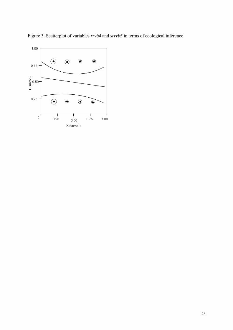
(population or sample) level. Type 3 variable data were put in the artificial population according to their observed distribution. Type 2 variables will also be considered in the aggregate level, because this may give both significant false positive, negative and zero correlations resulting from the aggregation. The results of independent simulations, four in each category, with different random number seeds can be seen in Table 6. Table 6. It can be seen from Table 6 that artificially generated random variables in the population level produce in a 2 percent random sample of the population in about 9-10 percent of the cases a false significant association by chance. Since several tests were made, this phenomenon is related to the multiple testing problem (Westfall and Young, 1993). Demographic variables from a general social survey (Type 3 variables) are correlated in a 2 percent sample of the population as expected in about 76-81 percent of the cases. While Type 1 and Type 2 variables are independent by construction in the individual (population) level, they produce an artificial significant association in the aggregate level in about 25-100 percent of the cases with the sum aggregation function, and in about 2-19 percent with the mean aggregate function, depending on the spatial distribution of the population. Type 3 variables are dependent in the individual (population) level in about 76-81 percent of the cases and they produce significant association in the aggregate level in about 71-100 percent of the cases with the sum aggregation function, and in about 5-24 percent with the mean aggregate function, depending on the spatial distribution of the population. The significance of associations among nominal variables were measured with the Pearson’s chi-squared statistic, among nominal and scale variables with the F-test, and among two scale variables the significance of the Pearson’s correlation coefficient was used, respectively. An example will show how the various methods work in practice. Two structured random variables rrvb4 and srrvb5 (Table 5) with binomial probability 0.2, 0.2, 0.4, 0.6, 0.8, 0.8, 0.6, 0.4, 0.2, 0.2, and 0.8, 0.8, 0.2, 0.2, 0.8, 0.8, 0.2, 0.2, 0.8, 0.8 by precinct, respectively, were analyzed, assuming a uniform(1,100) random distribution of the population by precinct. These variables are independent by construction in the population level. In a 2 percent sample the analysis of a 2x2 table with variables srrvb4 and srrvb5 the hypothesis of independence is not rejected (exact 2-sided P=0.112). The parameters of the saturated hierarchical loglinear model are λ11

AAB = 0.000373, standard error =0.02408, λiA = 0.21659, standard error = 0.02408 and

λjB . =0.245203, standard error = 0.02408. The model of independence ln mij=μ+λi

A + λjB fits

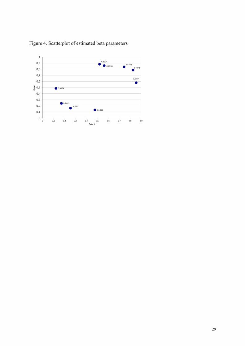
well, where A denotes variable srvbn4a and B denotes srvbn4b, and the population level by construction independence between variables rrvb4 and srrvb5 remained in the 2 percent sample level. On the basis of the marginal distributions, however, the data pattern is different. With the program EzI v2.20 1/12/1999 (King, 1999) it can be seen that the data in terms of ecological inference are located in two different areas of the data graph (Figure 3), where the variables rrvb4 and srrvb5 are denoted by X and T in the program output, respectively. The estimated beta parameters are (0.5627, 0.8593), (0.2560, 0.1627), (0.8258, 0.7873), (0.1241, 0.4854),

11

(0.8557, 0.5774), (0.1725, 0.2413), (0.7450, 0.8382), (0.4787, 0.1303), (0.5206, 0.8824), by precincts, respectively, (Figure 4.), where betas are estimated proportion of rrvb4 and srrvb5. Figure 3. Figure 4. With this approach it seems that both the observed data and the estimated parameters of the two variables rrvb4 and srrvb5 are separated, i.e. they are not closely related, which is in relation to the conclusion derived from the 2 percent sample and that from the population. On the basis of the marginal distributions, however, the data pattern is different. With the program EzI v2.20 1/12/1999 (King, 1999) it can be seen that the data in terms of ecological inference are located in two different areas of the data graph (Figure 3), where the aggregate variables rrvb4 and srrvb5 with the mean function are denoted by X and T in the program output, respectively. The estimated beta parameters are (0.5627, 0.8593), (0.2560, 0.1627), (0.8258, 0.7873), (0.1241, 0.4854), (0.8557, 0.5774), (0.1725, 0.2413), (0.7450, 0.8382), (0.4787, 0.1303), (0.5206, 0.8824), by precincts, respectively, (Figure 4), where betas are estimated proportion of rrvb4 and srrvb5. With this approach it seems that both the observed data and the estimated parameters of the two variables rrvb4 and srrvb5 independent by construction are separated, i.e. they are not closely related, which is in line with the conclusion derived from a 2 percent sample. Another example is the analysis of the relationship between two variables age group and family status coming from Hungarian population and survey data. Age group (agegrp1) and family status (famistat) are closely related. In a 2 percent sample the hypothesis of independence is rejected (asymptotic 2-sided P=0.000). The interaction parameters of the fitted hierarchical loglinear model are between –1.10543 and 1.95867 with stardard errors between 0.11150 and 0.29861. This result is in accordance with the fitted saturated model ln mijk=μ+λi

A + λjB + λij

AAB, where A denotes variable agegrp1 and B denotes famistat. On the basis of the marginal distributions, assuming a uniform(1,100) random distribution of the population by precinct, the data pattern is again different. With the program EzI v2.20 1/12/1999 (King, 1999) it can be seen that the data in terms of ecological inference are located virtually in one area of the data graph (Figure 5), where the aggregate variables agegrp1 (age group) and famistat (family status) with the percentage above 0 function are denoted by X and T in the program output, respectively. The estimated beta parameters are (0.2992, 0.1047), (0.3007, 0.0993), (0.2992, 0.1008), (0.3074, 0.1045), (0.3015, 0.0985), (0.3058, 0.1103), (0.3029, 0.0971), (0.3062, 0.1099), (0.3077, 0.1082) , (0.3014, 0.0945), by precincts, respectively, (Figure 6), where betas are estimated proportion of agegrp1 and famistat. Figure 5. Figure 6. It can be concluded that from individual level (2 percent sample) and aggregate level data similar conclusions may be drawn with traditional statistical methods and King’s method. The combination of both aggregate and individual data has also extensively been investigated by Gelman. He has proposed a hierarchical model in R and Bugs for the solution of the problem at hand (Gelman, 1995, 2003; Gelman, 2006). The Markov Cahin Monte Carlo

12

method was invertigated in spatial data analysis practice by Gilks et al. (1998). The combination of both aggregate and individual data has also extensively been investigated by Carlin and Louis (Carlin, 2000). The use of hierarchical modelling in spatial data analysis was extensively investigated by Banerjee (2004). Jackson has developed a software in R called ecoreg (Jackson, 2006a) that is suitable for amendment of the inference with traditional methods from aggregate data. Jackson states that individual-level inference from aggregate data alone can be subject to bias due to confounding and other possible errors such as model mis-specification or lack of information, but incorporating individual-level data can reduce these biases (Jackson et al., 2006b). Jackson showed how this can be done by supplementing the aggregate data with small samples of data from individuals within the areas, which directly link exposures and outcomes (Jackson, 2005). Results Adult education is of growing importance and the determinants of participation is crucial in economic development. The effect of income, educational level, urbanization and unemployment rate was analyzed on Hungarian adult education at the aggregate level. The model examined is Logit(pij)=μi+Σrαrxir+Σrβrzijr+γsij Where xir are group-level covariates, and zijr are individual-level covariates. The group-level covariates include income, educational level, urbanization and unemployment. The individual-level covariates include the same variables, i.e. income, educational level, urbanization and unemployment. The baseline risk μi is considered as a random effect across areas. This accounts for the remaining overdispersion and heterogeneity between areas, after adjusting for observed area-level variables. The random effect also allows the borrowing of information across areas and can stabilize estimation from areas with small populations (Jackson, 2006a; Richardson and Best, 2003). Logistic regression analysis based on this model provided the corresponding odds-ratios (OR) showing very large value (14,29) for the educational level at the aggregate level. Individual level logistic regression analysis revealed also large but relatively much smaller (1,27) OR for the educational level. A combined analysis of both aggregate and individual level data with the ecoreg programme in R provided a relatively high OR but much smaller than that of the aggregate level for educational attainment (Table 7.) Table 7 The conclusion is that participation in adult education is largely influenced by existing educational level. In adult education mostly qualified people take part. This is a very unfavorable feature of the existing educational system (Molnár, 2006). This result is confirmed with several other traditional statistical methods at the individual level too. Discussion

13

Ecological fallacy is a common problem when correlation analysis is made. Similarly, Simpson’s paradox frequently occurs in the analysis of multiway contingency tables in social sciences, clinical trials, epidemiological and marketing research. The similarity between ecological fallacy and Simpson’s paradox is in the controversy between the results of analyzing individual level and aggregated data. King proposed a solution to the ecological problem. He emphasized the importance of certain characteristic features that a solution should be met. He used an amended Goodman’s regression method, which is based on a straightforward and unrestricted linear regression with some assumptions. As Wakefield stated it is not true that nothing can be gained from ecological data with respect to the estimation of the individual level odds ratio, because some information is contained within the ecological level data. Although in real life individual level data in some cases is difficult to collect, Wakefield proposed a combination of both aggregate and individual level data for finding a more accurate solution to the ecological problem. He investigated, for instance, the beneficial effect of taking a 5 percent sample of observations from within precinct level tables on ecological inference. He used the MCMC method in R and WinBugs and he sampled of blacks and whites of fixed sizes, and then sampled from the rows (one for blacks, one for whites) using a hypergeometric distribution for each (Wakefield, 2004). A simulation study may help to find a way to reduce the cost of sample survey in relation to ecological fallacy. Although theoretically several data patterns may result ecological fallacy, in practice it may be useful to examine how various simulated data patterns “behave” in this respect in order to arrive at a conclusion. The analysis of artificial, randomly generated population (individual level) data results in a conjecture supported by examples that both false negative and false positive results may easily occur, both for individual and aggregated level data. when both individual and area aggregated data are examined. The significant positive or negative results may be related to any town, village or precinct. Therefore great caution is needed when analyzing area aggregated data An artificial populations of 100,000 have been created in such a way that people were randomly allocated to 100 towns and villages according to the lognormal distribution (Population 1) with parameters (2,1.1). The resulting population is mostly in small villages, some live in larger towns and a few in large towns. Rounding of fractional numbers helped to eliminate fractional people when the corresponding number was not an integer. Another artificial population of 100,000 have also been created in such a way that people were randomly allocated to 100 precincts according to the normal distribution (Population 2) with parameters (50,18). The correlation among randomly generated variables at the individual level can be spuriously significant, but less frequently than after aggregation. Artificially created random data patterns may result in false positive of false negative relationships between variables both in the individual and the aggregated level. The significant positive or negative results may be related to any town, village or precinct. Although great caution is needed when analyzing area aggregated data Wakefield’s proposal may be an important step towards valid ecological inference. Despite of the difficulties it is possible in many situation to conduct some sort of

14

survey to assess the situation. Although taking a 5 percent sample of observations from within precinct level tables on ecological inference is frequently too expensive, there are alternative ways to receive information about the real processes. Various proposals can be made about amending the ecological inference and, therefore receiving valid information about ecological data mostly with the application of certain quality assurance measures and at the expense of a slight or moderate increase in costs. 1. Since the significant positive or negative results at the aggregate level, even when using the same, but numerically different, random variables at the individual level, may appear in any area (town, village or precinct) due to random variations, the most straightforward and cheap proposal is to take a conventional multistage stratified sample and conduct a survey on the variables in question, and then use the information in the sample for the assessment of ecological relationships. 2. It is possible to make a more detailed analysis of data with collecting sample data through a spatial sampling plan. The conventional multistage stratified sampling plan frequently starts with selecting the layer of the city and then a separate layer of large towns, and only after the layer of smaller towns and villages in various spatial settings. This sampling plan should be reversed in such a way that the first step be a spatial (area) sampling, and within that framework the conventional multistage stratified sampling plan be made. The advantage of such a sampling plan is that it makes survey data applicable to deeper spatial analysis concerning ecological inference. For example regional or county level survey data may help finding a more accurate relationship between variables both in the individual and the aggregate level. Or any other area blocks can be created according to the needs. This way a larger sample is needed than it is customary in a sample survey but still with moderate expenses. 3. It is also possible to concentrate to certain geographic areas where the survey should be conducted. The reason of the selection of certain areas may be, for example, a special interest about these areas or a need for the validation of data outliers. This way relatively cheap information can be collected about certain areas which are of crucial importance. 4. Another way of amending ecological inference is to aggregate precincts or towns and villages into larger areas, making comparison of individual and aggregate data more feasible. This way some information is lost about the very detailed geographic data, but far more accuracy can be achieved in ecological inference. 5. A further possibility is to use a spatial smoothing algorithm and to create new spatial blocks on the basis of smoothed data or that of finding spatial barriers by Monmonier’s algorithm (Solymosi et al, 2005). The sample survey can then be designed according to these relevant areas, and the ecological inference can be made accordingly. 6. The combination of likelihoods as proposed by Wakefield or weighted regression, where the variance is reduced by increased amount of information from a sample survey as proposed by King and Wakefield can be used. Also as information gathered increase, the application of Bayesian methods may be also very fruitful. More research and software development is needed to provide a user friendly combination of ecological and survey data. Wakefield used the R package MCMCpack, available from CRAN implementing ecological inference for 2x2 tables using a Bayesian hierarchical model (Wakefield, 2004).

15

7. Gelman used extensively the Markov Chain Monte Carlo method and WinBugs for the solution of hierarchical regression problems with multilevel modelling (Gelman, 1995, 2003; Gelman, 2006). 8. The Markov Chain Monte Carlo method was extensively investigated and used in spatial data analysis practice by Gilks et al. (1998). 9. The combination of both aggregate and individual data was also extensively investigated and used with the help of hierarchical regression with multilevel modelling by Carlin and Louis (Carlin, 2000). 10. The use of hierarchical modelling in spatial data analysis was also extensively investigated with the help of hierarchical regression with multilevel modelling by Banerjee (2004). 11. Jackson’s user friendly ecoreg programme in R will certainly pave the way of the wider application of the combination of aggregate and individual level data. Recent developments in Bayesian data analysis seem to make it possible to solve or at least relatively easily manage the problem of ecolgocial fallacy. 12. With easier management of the ecological fallacy problem one may think of further development of data collection and data analysis methods. In addition to the analysis of aggregate data, special sampling designs may help the analyst to have a deeper insight into the phenomena investigated. One may have a traditional general social survey with a sample of size N. Or one may concentrate with a sample survey to certain spatial areas in which the variance of the most interesting variables are large. Or one may concentrate with a sample survey to certain spatial areas where the information is scarce. The sophisticated statistical methods developed within the last ten years may then be used with an eye on these special sampling designs, and the new methods, to get out the most information from the data. This has also been investigated and discussed by Glynn al. (2006).

16

References Adolph, C. and G. King, G. With Herron, M.C. and K.W. Shotts (2003). A consensus on Agresti, A. (1990). Categorical data analysis. Wiley Banerjee, S., B. P. Carlin and A. E. Gelfand (2004). Hierarchical modeling and analysis of spatial data. Chapman and Hall/CRC Birch, M.W. (1963). Maximum likelihood in three-way contingency tables. J. Roy. Statist. Soc. B25:220-233. Bishop, Y.V.V, S.F. Fienberg, and P.W. Holland (1975). Discrete Multivariate Analysis. Cambridge, MA: MIT Press Carlin, B. P. and T. A. Louis (2000). Bayes and empirical Bayes methods for data analysis. Chapman and Hall/CRC Clogg, C.C. and S.R. Eliason (1987). Some common problems in loglinear analysis. Sociol. Methods Res., 15:4-44. Corder, J.K. and C. Wolbrecht (2004). Using prior information 5to aid ecological inference: a Bayesian approach. In Ecological Inference: New Methodological Strategies (eds. G. King, O. Rosen and M. Tanner). Cambridge: Cambridge University Press Durkheim, E. (1973). Az öngyilkosság. KJK, Budapest Edwards, D. (1995). Introduction to graphical modelling. Springer-Verlag, New York Fienberg, S.E. (1970). An iterative procedure for estimation in contingency tables. Ann. Math. Statist. 41:907-917. Gelman, A., J. B. Carlin, H. S. Stern and D. B. Rubin (1995; 2003). Bayesian Data Analysis. Chapman and Hall. Gelman, A., J., J. Hill (2006). Applied regression and multilevel models. In Press Gilks, W. R., S. Richardson and D. J. Spiegelhalter (1998). Markov Chain Monte Carlo in Practice. Chapman and Hall/CRC Glynn, A., J. Wakefield, M. S. Hadcock, and T. S. Richardson. (2006). Alleviating linear ecological bias and optimal design with subsample data. Manuscript. Haberman, S.J. (1972). Algorithm AS 51. Log-linear fit for contingency tables. Applied Statistics 21:218-224. Haneuse, S. and J. Wakefield (2004). Ecological inference incorporating spatial dependence. In Ecological Inference: New Methodological Strategies (eds. G. King, O. Rosen and M. Tanner). Cambridge: Cambridge University Press Jackson, C. (2005). Improving ecological inference using individual-level data. Statistics in Medicine. In Press. Jackson, C. (2006a). Ecological inference with R: the ecoreg package. Version 0.1.1. Jackson, C., N. Best, and S. Richardson. (2006b). Hierarchical related regression for combining aggregate and survey data in studies of socio-economic disease risk factors. To be published. King, G. (1997). A solution to the ecological inference problem. Princeton University Press second-stage analyses in ecological inference models. Political Analysis, 86-94. King, G. (1999). EzI v2.20 computer software Knorr-Held, L. and N.G. Best (2001). A shared component model for detecting joint and selective clustering of two diseases. J. Roy. Statist. Soc. A164:73-85. Mészáros, J. (1990). Simpson Paradoxon (Intés a kereszttáblák aggregálásától), Budapest, Hungarian Academy of Sciences, National Institute of Sociology, 32 pages. Mészáros J. and I. Szakadát (2005a). Magyarország Politikai Atlasza. Gondolat K., Budapest Mészáros, J., D.L. Molnár, J. Reiczigel, and N. Solymosi (2005b). Introduction to spatial statistics. (In Hungarian; Book in preparation)

17

Molnár, L.D. (1991) Loglinear Discriminant Analysis. The American Statistician. November, Vol. 45. No. 4.:339. Molnár, L.D., J. Reiczigel, T. Rudas and É. Gárdos (1992). Monte-Carlo and Bootstrap Methods for the Analysis of Multidimensional Contingency Tables. TÁRKI Preprint 1992/4. Molnár, D.L. (2004). General Social Survey, Budapest. Sample size 1000. Manuscript Molnár, D.L. (2006). Adult education in Hungary. Sample size 1000. Manuscript Plackett, R.L. (1977). The marginal totals of a 2x2 table. Biometrika, 64:37-42. Radelet, M. (1981). Racial characteristics and impositions of the death penalty. Amer. Sociol. Rev. 46: 918-927. Richardson, S. and N. Best (2003). Bayesian hierarchical models in ecological studies: of health-environment effects. Environmetrics, 14:45-59. Rudas, T. (1982) The Analysis of Contingency Tables. Lecture Notes, Eotvos University, Budapest, second printing: 1993 (Hung.) Rudas, T. (1990) DISTAN for discrete statistical analysis. in: Faulbaum, Haux, Jockel (eds.) SoftStat'89, Fortschritte der Statistik-Software 2, 144-154, Gustav Fischer Verlag, Suttgart, New York. Rudas, T. (ed.) (1992) DISTAN 2.0 Manual. Social Science Informatics Center, Budapest. Rudas, T. (1998). Odds Ratios in the Analysis of Contingency Tables. Sage Publ., Thousand Oaks, CA Rudas, T. (2002) Canonical representation of log-linear models. Communications in Statistics (Theory and Methods), 31, 2311-2323. Rudas, T. (2005) Odds and odds ratios, in: Everitt, B, Howell, D. (eds). Encyclopedia of Statistics in Behavioral Science, 1462-1467,Wiley. Simpson, E.H. (1951). The interpretation of interaction in contingency tables. J. Roy. Statist. Soc. B13:238-241. Skene, A.M. and J.C. Wakefield (1990). Hierarchical models for multi-centre binary response studies. Statist Med, 9:919-929. Solymosi, N., J. Reiczigel, A. Harnos, J. Mészáros, L.D. Molnár and F. Rubel (2005). Fidning spatial barriers by Monmonier’s algorithm. Presented at ISCB Conference, Szeged, Hungary Wakefield, J. (2004). Ecological inference for 2 x 2 tables. J. Roy. Statist. Soc. A167: 385-445. Westfall, P.H. and S.S. Young (1993). Resampling-based multiple testing. Wiley

18

Table 1. The ecological inference problem

Voting decision Race of voting person Democrat Republican No vote Total Black ? ? ? 55054 White ? ? ? 25706 Total 19896 10936 49928 80760

19

Table 2. The ecological inference problem in general form

X Y=0 Y=1 Total 0 Y0i N0i 1 Y1i N1i Total Ni-Yi Yi Ni

20

Table 3. Notation for the situation having both individual survey data and aggregate marginal data in area i

x Survey data Aggregate data Y=0 Y=1 Total Y=0 Y=1 Total 0 z0i m0i N0i-m0i 1 z1i m1i N1i-m1i mi-zi zi mi Ni-mi-(yi-zi) yi-zi Ni-mi

21

Table 4. The death penalty example (frequencies)

Penalty Defendant white Death Other Total Victim white 19 132 151 Victim black 0 9 9 Total 19 141 160 Defendant black Death Other Total Victim white 11 52 63 Victim black 6 97 103 Total 17 149 166

22

Table 5. Probability parameters of simulated binomial type 2 structured variables by town, settlement or precinct

Town, settlement or precinct Variable 1-10 11-20 21-30 31-40 41-50 51-60 61-70 71-80 81-90 91-100 srrvb1 0.2 0.2 0.2 0.2 0.2 0.8 0.8 0.8 0.8 0.8 srrvb2 0.8 0.8 0.8 0.8 0.8 0.2 0.2 0.2 0.2 0.2 srrvb3 0.2 0.4 0.6 0.8 0.8 0.8 0.8 0.6 0.4 0.2 srrvb4 0.2 0.2 0.4 0.6 0.8 0.8 0.6 0.4 0.2 0.2 srrvb5 0.2 0.8 0.2 0.8 0.2 0.8 0.2 0.8 0.2 0.8 srrvb6 0.8 0.8 0.2 0.2 0.8 0.8 0.2 0.2 0.8 0.8

23

Table 6. Significance of measures of associations in four independent simulations in individual (population), aggregate and sample survey level with Type 1 simple random variables, Type 2 structured random variables, and two independent simulations with Type 3 observed variables % of significant association measures (p<0.05) Simul-ation

Variable type Spatial distribution of population

Aggregate by sum function

Aggregate by mean function

Individual (sample survey)

1-4 Type 1 and 2 Normal(50,17) 78-100 % 10-19 % 9-10 % 1-4 Type 1 and 2 Lognormal(2,1.1) 100 % 11-18 % 1-4 Type 1 and 2 Uniform(1,100) 25-99 % 2-9 % 1-4 Type 3 Normal(50,17) 100 % 5-14 % 76-81 % 1-4 Type 3 Lognormal(2,1.1) 100 % 24 % 1-4 Type 3 Uniform(1,100) 71-76 % 5-14 %

24

Table 7. Results of analysis with the ecoreg programme in R Aggregate data Model: adulte ~ incomea + educa, + binary = ~ urbana + unempa Aggregate-level odds ratios: OR l95 u95 (Intercept) 1.11 2.59e-02 4.75e+01 Incomea 0.94 8.74e-01 1.02e+00 Educa 14.29 7.17e-18 2.84e+19

Individual-level odds ratios: OR l95 u95 Urbana 0.32 0.14 0.70 Unempa 0.04 0.0001 14.60

-2 x log-likelihood: 152.41 Individual data Model: adulte ~ incomei + educi + urbani + unempi Aggregate-level odds ratios: OR l95 u95 (Intercept) 0.03 0.01 0.08

Individual-level odds ratios: OR l95 u95 Incomei 1.00 0.87 1.16 Educi 1.27 1.19 1.35 Urbani 0.62 0.46 0.85 Unempi 1.04 0.64 1.70

-2 x log-likelihood: 1235.073 Combined aggregate and individual data Model: adulte ~ incomea + educa, binary = ~ urbana + unempa, iformula = adulte ~ incomei + educi + urbani + unempi, groups=region code, igroups=region code Aggregate-level odds ratios: OR l95 u95 (Intercept) 0.71 0.59 0.85 incomea 1.0 0.97 1.04 educa 1.01 0.99 1.02

Individual-level odds ratios: OR l95 u95 Urbani 0.70 0.54 0.92 Unempi 0.90 0.57 1.43

-2 x log-likelihood: 1459.586

25

Fig 1. Schematic representation of the ecological problem

26

Figure 2.a. Schematic representation of Simpson’s paradox

27

Figure 2.b. Another schematic representation of Simpson’s paradox

28

Figure 3. Scatterplot of variables rrvb4 and srrvb5 in terms of ecological inference

29

Figure 4. Scatterplot of estimated beta parameters

0,4854

0,2413

0,1303

0,5774

0,83820,8824

0,7873

0,1627

0,8593

0

0,1

0,2

0,3

0,4

0,5

0,6

0,7

0,8

0,9

1

0 0,1 0,2 0,3 0,4 0,5 0,6 0,7 0,8 0,9

Beta 1

Bet

a 2

30

Figure 5. Scatterplot of variables age group and family status in terms of ecological inference

31

Figure 6. Scatterplot of estimated beta parameters

0,0971

0,0945

0,1045

0,10820,1103

0,1099

0,0985

0,1008

0,0993

0,1047

0,092

0,094

0,096

0,098

0,1

0,102

0,104

0,106

0,108

0,11

0,112

0,298 0,299 0,3 0,301 0,302 0,303 0,304 0,305 0,306 0,307 0,308 0,309

Beta 1

Bet

a 2