improving climate model representations of snow hydrology

Environmental Modelling & Software 14 (1999) 327–334

Improving climate model representations of snow hydrology

Susan Marshalla,*, Robert J. Oglesbyb, Kirk A. Maaschc, Gary T. Batesd

a Department of Geography and Earth Sciences, University of North Carolina, Charlotte, NC 28223, USAb Department of Earth and Atmospheric Sciences, Purdue University, West Lafayette, IN 47907, USA

c Institute of Quaternary Studies and Department of Geological Sciences, University of Maine, Orono, ME 04469, USAd Climate Diagnostic Center, NOAA, Boulder, CO 80307, USA

Received 26 April 1998; received in revised form 15 July 1998; accepted 15 July 1998

Abstract

In this study previous work that led to an improved representation of snow albedo in global climate models is expanded toinclude regional simulations of snow cover over three distinctly different regions of the United States. We also discuss broadeningour work in snow cover parametrization to include representation of the following processes: (i) the ‘dirtiness’ of snow (due todust and other particulate loading); (ii) partitioning of energy between melt, evaporation of meltwater, and refreezing within thesnow pack; (iii) heat added to a snowpack by rain; and (iv) the vertical temperature profile within a snowpack. In addition, a newparameter, called ‘WFLUX’, is introduced as a useful glaciological parameter that is based on the net energy available for snowmelt.The snow hydrology formulation of Marshall and Oglesby is implemented into two widely used climate models: a global GCM,the NCAR CCM3/LSM, and a regional climate model, the RegCM2 version of MM4. A suite of new simulations has been madewith RegCM2 for three regions of the United States for the 1992–1993 snow season. The regions of interest include the westernUS/Rocky Mountain region, the region surrounding the Great Lakes and the northeastern United States. Calibration and validationof the new snow hydrology is accomplished by comparison to available ground and satellite based datasets of snowcover, includingboth mean conditions and year-to-year variability. The goal is not just to improve the simulation of the present-day seasonal cycle(which is reasonably well simulated by many current climate models) but also to improve the predictive capability of models whenused to address questions of past climate (especially those involving glaciation) and possible future climatic change. 1999 ElsevierScience Ltd. All rights reserved.

Keywords:Snow hydrology; Climatology; Climate modeling

Software availability

Program title: NCAR CommunityClimate Model, version 3

Developers: National Center forAtmospheric Research,Climate and GlobalDynamics Division(NCAR/CGD)

Contact address: NCAR/CGD, Box 3000,Boulder, CO 80307

First available: CCM3 available May1996

Hardware: CRAY running UNICOSor advanced workstations(IBM, SUN, SGI, DEC)

* Corresponding author. E-mail: [email protected]

1364-8152/99/$ - see front matter 1999 Elsevier Science Ltd. All rights reserved.PII: S1364-8152 (98)00084-X

Software required: C preprocessor,FORTRAN compiler,IMSL numerical libraries(or equivalent)

Program language: FORTRANProgram size: 3 MbAvailability: Access via anonymous ftp:

ftp.ucar.edu insubdirectory /ccm or viaWorld Wide Web underthe URL:http://www.cgd.ucar.edu/cms

Program title: Regional Climate Model,version 2 (RegCM2)

Developers: Giorgi et al. (1993a, b)Contact address: CDC/NOAA, Boulder, CO

80309, USAFirst available: RegCM2 available May

328 S. Marshall et al. /Environmental Modelling & Software 14 (1999) 327–334

1993Hardware: CRAY running UNICOS

or advanced workstations(IBM, SUN, SGI, DEC)

Software required: C preprocessor,FORTRAN compiler,IMSL numerical libraries(or equivalent)

Program language: FORTRANProgram size: 1.2 MbAvailability: Available upon request—

contact G.T. Bates([email protected])

1. Introduction

The extent and duration of seasonal snow cover playsan important role in determining local, regional, and glo-bal climates. In addition, snowfall and snow cover are acrucial element in determining the presence and extentof ice sheets and glaciers. For example, a positive netannual snow accumulation (more snow falls during theyear than melts) is a requirement for a glacier or icesheet to form and grow. The magnitude of the net snowaccumulation determines the rate at which a glacier orice sheet can grow (or conversely, if the ice has advectedhorizontally into a region with new snow ablation, howquickly it will melt). Successful simulation of the netsnow accumulation is therefore of paramount importancein any climate modeling study (a requirement for inputto ice sheet models). Unfortunately, representation of thephysical processes that determine snow accumulationand snow melt (ablation) are crudely handled in manycurrent climate models (and are consequently a potentialweakness of ice sheet model simulations).

An accurate account of the annual net balance of snowinvolves computation of both the amount of snow thatfalls, and the amount of snow that melts. Computationof snowfall requires accurate treatment of the large-scaleflux of water, as well as detailed cloud microphysics,and is not explicitly considered further in our work.Computation of snow melt requires accurate treatmentof snow albedo, and the thermodynamics of a snow pack.In this paper we describe two steps we have taken toimprove the simulation of snow hydrology in global andregional climate models. The first was an improvementof the representation of snow albedo in climate models(Marshall, 1989; Marshall and Oglesby, 1994). Thesecond was improving the thermodynamical represen-tation of heating and phase changes within a snowpack.Model runs using these new snow hydrology compo-nents were validated using an observed dataset that is ablend of surface and satellite measurements. In addition,we introduced a new climate model parameter, WFLUX,

that is useful for glaciological studies. WFLUX is a mea-sure of the amount of energy available for snow melt ata given time.

The focus of this paper is to describe regional studiesof the modeled snow hydrology and to discuss on-goingefforts in the parametrization of key snow melt pro-cesses. For the former, we will focus on three areas: (a)western United States covering the Rocky Mountainsand high plains, (b) upper Mississippi River basin andthe Great Lakes, and (c) northeastern United States andeastern Canada. Each region represents a unique set ofsurface characteristics and forcings on the snowpack. Wemodeled the three regions for the same winter/springseason (December 1992 through May 1993), forcing thelateral boundaries of the regional model with ECMWFreanalyses. All regions were run both with the standardland surface package of the regional climate model(BATS, see below, Dickinson et al., 1993) and with thesnow albedo routine of Marshall and Oglesby (1994).Calibration and validation were accomplished by com-parison with available observations, including surfaceand satellite-generated fields.

Our primary objectives are to (1) investigate theeffects of the snow hydrology changes of Marshall andOglesby (1994) on the simulation of a seasonal snow-pack over several regions of the United States and (2)use the results of these regional studies to drive theSNTHERM point mass and energy balance model of Jor-dan (1996) in order done to examine in more detail therole of melt energy partitioning, meltwater evaporation,rain-on-snow events and vertical temperature structureof the snowpack on the snow surface energy budget andsnow-atmosphere feedbacks. The hope is to eventuallyincorporate these critical snowmelt processes andeffects, in a sufficiently simplified manner, into theregional (and global) climate models.

2. The climate models

2.1. NCAR global GCMs

Our primary modeling tool to date has been theNational Center for Atmospheric Research (NCAR) ser-ies of global general circulation models (GCMs) calledthe Community Climate Model (CCM). This researchhas spanned versions of this model from CCM0(Marshall et al., 1994), CCM1 (Marshall and Oglesby,1994), and CCM2 to the most recent version, CCM3(Kiehl et al., 1996). CCM3 forms the core componentof the new NCAR Climate System Model (CSM) whichalso includes a land surface model (LSM) and a varietyof ocean and sea ice options. The LSM (Bonan, 1996)uses a slightly modified version of the snow albedo for-mulation of Marshall and Oglesby (1994).

CCM0 and CCM1 have a spectral horizontal resol-

329S. Marshall et al. /Environmental Modelling & Software 14 (1999) 327–334

ution of R15 (4.5° latitude by 7.5° longitude), with 12levels in the vertical, while CCM2 and CCM3 have aspectral horizontal T42 resolution (2.8° latitude by 2.8°longitude). CCM2 and CCM3 also have considerablyimproved physical parametrizations including modifi-cations to the treatment of radiative transfer, especiallythe inclusion of trace gases and background aerosol,improvements to the parametrization of cloud opticalproperties and modifications to the hydrologic cycle,especially the estimation of the atmospheric boundarylayer height and the treatment of deep moist convection(see Kiehl et al., 1996 for details).

2.2. RegCM2/BATS regional climate model

We will also present simulations using a regional cli-mate model, RegCM2, developed by Giorgi et al.(1993a,b). This regional climate model is based on theNCAR–Penn State Mesoscale Model version 4 (MM4)but with surface and near-surface parametrizations ofradiative and heat fluxes designed for use specifically inclimate studies. The surface fluxes of sensible heat andwater are determined using the Bio-Atmosphere TransferScheme (BATS) of Dickinson et al. (1993), to which hasbeen added the snow albedo formulation of Marshall andOglesby (1994). This model can be run at a horizontalresolution of about 20 km up to about 100 km, andrequires lateral forcing provided either from observationsor a GCM.

3. Observational datasets

Observational datasets of snow cover and snow depththat are both spatially and temporally continuous con-tinue to be limited in number. The primary productyielding an estimate of snowcover that is used for vali-dation of the model snow hydrology results is the seriesof NOAA/NESDIS weekly northern hemisphere snowcharts. These composite snow charts are based on datafrom the visible channel of the Advanced Very HighResolution Radiometer (AVHRR) (Robinson, 1993).AVHRR data are limited by cloud cover, thus use is alsomade of data from the NIMBUS-7 Scanning Multichan-nel Microwave Radiometer (SMMR) and DMSP SpecialSensor Microwave/Imager (SSMI) datasets (Goodisonand Walker, 1993). These microwave channels candetect snow cover even when clouds are present. Theadvantage of this dataset is that multi-year data are nowavailable such that both mean snow cover and interan-nual variability can be assessed. The disadvantage is thatthese charts provide information on snow extent onlyand not snow depth.

To obtain estimates of snow depth we look to: (a) theNIMBUS-7 SMMR dataset of snow depth (Chang et al.,1992), which provide a global coverage of monthly aver-

age snow depths from November 1979 through August1987, (b) first-order snow recording stations (such as theUSHCN/D stations distributed by CDIAC), which pro-vide spatially discontinuous, but temporally continuousmeasures of snow depth, snowfall, precipitation and tem-perature, and (c) the Foster and Davy (1988) US AirForce monthly snow depth climatology.

4. Developing a new snow hydrology

4.1. Step 1: snow albedo and snowcover fraction

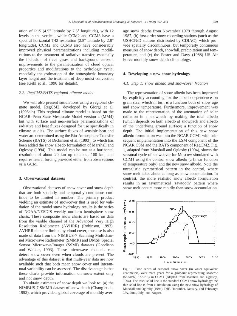
The representation of snow albedo has been improvedby explicitly accounting for the albedo dependence ongrain size, which in turn is a function both of snow ageand snow temperature. Furthermore, improvement wasmade to the representation of the attenuation of solarradiation in a snowpack by making the total albedo(which depends on both albedo of snowpack and albedoof the underlying ground surface) a function of snowdepth. The initial implementation of this new snowalbedo formulation was into the NCAR CCM1 with sub-sequent implementation into the LSM component of theNCAR CSM and the BATS component of RegCM2. Fig.1, adapted from Marshall and Oglesby (1994), shows theseasonal cycle of snowcover for Moscow simulated withCCM1 using the control snow albedo (a linear functionof temperature only) and the new snow albedo. Note theunrealistic symmetrical pattern in the control, wheresnow melt takes about as long as snow accumulation. Incontrast, the more realistic snow albedo formulationresults in an asymmetrical ‘sawtooth’ pattern wheresnow melt occurs more rapidly than snow accumulation.

Fig. 1. Time series of seasonal snow cover (in water equivalentcentimeters) over three years for a gridpoint representing Moscow(55.50°N; 37.50°E) in CCM1 (adapted from Marshall and Oglesby,1994). The thick solid line is the standard CCM1 snow hydrology; thethin solid line is from a simulation using the new snow hydrology ofMarshall and Oglesby (1994). DJF, December, January, and February;JJA, June, July, and August.


Subsequent simulations of this formulation into theregional climate model show similar results. Since theBATS surface package already contains a suitablesnowcover fraction computation, the differencesbetween the control and albedo simulations are attributedsolely to the snow albedo formulation. Fig. 2 shows theresults from the regional simulation over the westernUnited States. The snow albedo parametrization showshigher surface snow albedos during the melt season andtherefore, less energy absorbed at the surface and henceless snowmelt. The timing of complete melt is extendedby a few days to a couple of weeks. There is little changeevident in the accumulation season. The results are simi-lar for the other regions.

4.2. Step 2: melt season processes

We have focused on several other features of the snowhydrology that are important to the accurate parametriz-ation of snow melt. These include: (i) the ‘dirtiness’ ofsnow (due to dust and other particulate loading); (ii) par-titioning of energy between melt, evaporation ofmeltwater, and refreezing within the snow pack (currentparametrizations usually assume all available energygoes into melt only); (iii) the vertical temperature profilewithin a snowpack; and (iv) heat added to a snowpackby rain. The first two of these processes are discussedbelow.

One feature of the snow albedo parametrization ofMarshall (1989) is the ability to specify the presence oflight-absorbing impurities in the snowpack and include

Fig. 2. Seasonal cycle of water equivalent snow depth over the West-ern United States region. Comparison is made between the controlsimulation of RegCM2 (‘CONTROL’, thick solid line), a simulationof RegCM2 using the snow albedo parametrization of Marshall andOglesby (1994) and assuming pure snow (‘ALBEDO’, thin solid line),and a simulation using the new albedo parametrization but using aconcentration of 33 106 ppmv soot in the snow pack (thin dashedline).

the effects of such on the snow albedo. In the currentregional simulations, the snow cover is assumed to be‘pure’ snow (free of any light-absorbing impurities).Most all mid-latitude locations show some degree ofimpurities in the snow (Chy’lek, 1983), even the snowin Antarctica reveals measurable levels of particulates inthe snow (Warren and Clarke, 1990). Therefore, wewould expect that our computed ‘pure’ snow albedosmay be higher than observed. This may be a reason forthe higher albedos than that seen in the CONTROLsimulation, since the BATS parametrization of snowalbedo arbitrarily sets a level of impurities in the snow-pack to 33 10−6 ppmv of soot (soot here used as asurrogate for all light-absorbing impurities).

Fig. 2 also shows the results from the western USregion for three simulations: original model run(‘CONTROL’), modified model with new snow albedo(‘ALBEDO’) assuming pure snow, and modified modelwith new snow albedo and assuming a soot concen-tration in the snow of 33 10−6 ppmv (‘SOOT’), similarto the CONTROL simulation. As expected, the SOOTsimulation shows a lower surface albedo than in the caseof pure snow, but the albedos are still higher than theCONTROL run. The differences in the simulations,therefore, cannot be fully explained by thepresence/absence of impurities in the snow.

Improvement of the thermodynamical representationof temperature and phase changes of water at the surfaceand within a snowpack initially involved incorporatinga thermodynamic column model, which simultaneouslycomputed the vertically-integrated temperature of soiland snow for a gridpoint, into the Los Alamos versionof CCM0 (Marshall et al., 1994). This replaced the diag-nostic “heat balance” algorithm, used by most GCMs,with prognostic equations that describe the heat storageand thermal diffusion throughout the column (soil–snow–atmosphere). With the addition of snow to the col-umn, this allowed the surface and sub-soil temperaturesto respond more realistically to heat flow across theboundary and to more accurately account for the thermalde-coupling of the atmosphere and soil when snowcovered the surface. This kept the wintertime soil tem-peratures higher than had previously been simulated bythe model and dampened large fluctuations in the GCMcontinental skin temperature during Northern Hemi-sphere winter.

More recently, we have adopted the ideas of Kuz’min(1972) recognizing that conventional climate modelssuch as the NCAR CCM1 and RegCM2 estimate snowmelt through use of an ‘excess energy’. In this standardmodeling technique, the surface energy balance is com-puted iteratively in the normal fashion over snowcovered grid points. An estimate of sensible and latentheat fluxes is made, with the latter being equivalent toeither evaporation (or as is frequently the case,condensation). If the resultant surface temperature is


above freezing, the temperature is instead held at freez-ing, which leads to an energy surplus. This surplus, orexcess, energy is then assumed to be available to meltsnow (and can be used as the WFLUX parameter, seeSection 6 below). A small amount of snow is assumedto evaporate through sublimation at any temperature.

This approach is likely to underestimate the true evap-oration in the presence of melting snow because, inaddition to the (minimal) latent heat flux from a baresnow surface as computed via the standard approach, asdescribed by Kuz’min (1972), the melting snow releasesliquid water which is also subject to evaporation, andwhich can considerably enhance the total latent heat flux.The energy used to evaporate this additional water mustcome from the ‘excess energy’ and hence is not availableto contribute to snow melt. In addition, the melt watercan infiltrate the snow pack and refreeze thus addinglatent heat which warms the snow pack. The melt waterthat refreezes is not directly a part of net snow melt. Ingeneral, these effects are true even if a more sophisti-cated soil–vegetation–atmosphere scheme (SVAT) isused.

These processes can be accounted for conceptually bydefining a parameter called ‘a’ which describes that frac-tion of available energy which contributes to net snowmelt (i.e., does not evaporate water or lead to warmingof the snow pack). Empirical studies of snow cover sug-gest a value fora in the range 0.5–0.75 (e.g., Leavesleyand Stannard, 1989). Virtually all current climate modelsimplicitly use a 5 1.0, that is, all available energy asdefined above is applied to net snow melt (this includesthe work of Marshall and Oglesby, 1994). Because thelatent heat of vaporization is much larger than the latentheat of fusion,a 5 0.5, for example, means that onlyabout 10% of water from melting snow is evaporated.Fig. 3 shows snow cover averaged over the entire north-ern hemisphere as a function of season for simulationsusing NCAR’s CCM1 witha 5 1.0, 0.75, 0.50., and0.25. Note that the primary period of new snow accumu-lation (September through February) shows relativelylittle difference between the four cases, but as the latewinter and spring snow melt season proceeds, there isconsiderable variation, with highera values correspond-ing with greater rates of snow melt, and more overallsnow melt.

In order to provide a more predictive assessment ofa, we plan to use the latest version of the one-dimen-sional model of snowpack energy and mass balance,SNTHERM (Jordan, 1991, 1996). This model is basedon the one-dimensional energy and mass balance modelof Anderson (1976) (similar to many other current massbalance models of snow). The model solves the govern-ing equations for energy and mass within the snowpackand is forced at the upper boundary by basic meteoro-logical input (see Rowe et al., 1995) or in our work withoutput from the GCM. The main changes to the latest

Fig. 3. Seasonal cycle of the fractional Northern Hemisphere areaoccupied by snow (over land and sea ice) for three values of theaparameter (1.0, 0.75, and 0.50 as indicated on the figure).

revision (SNTHERM89.rev4, Jordan, 1996) includeimprovements to the computation of turbulent transfer,new snow density and snow compaction, snow graingrowth and snow albedo.

5. Model case studies

Satellite-derived and surface point snow cover esti-mates have been used to evaluate model simulations ofsnow cover; our goal so far has been to demonstrate thatthis is a reasonable approach. The following sectionbriefly describes two case study examples: the first com-paring model output to station snow depths over thenortheastern Unites States for the blizzard of March1993, the second example describes a comparisonbetween SMMR satellite products and model output ofsnow over the western US domain for a selectedmodel simulation.

Fig. 4 shows observed snow cover depths (shown asblack numbers) obtained from surface station data forthe March blizzard of 1993 (here showing the output forMarch 12 and 13, 1993) and simulated snow coverdepths (shown as contours) from RegCM2 for thosesame days. (Simulation data were taken from a North-eastern region simulation begun on November 1, 1992and run through June 1, 1993. RegCM2 was forced byECMWF reanalyses at the boundaries of the domain.)Both numbers represent water equivalent snow depths inmillimeters. Station data are generally reported in unitsof geometric snow depths. For comparison, we havearbitrarily, but reasonably, assumed a snow density of450 kg m−3 as a conversion. Note that the density vari-ations in melting snow can be large, therefore theobserved ‘water-equivalent’ snow depths represent a


Fig. 4. Snow depth over the Northeastern US domain for (a) March12, 1993 and (b) March 13, 1993, showing USHCN/D snow courseobservations (numbers, black) and the RegCM2 model (contours,gray). Depths are given in centimeters of water equivalent snow anda constant density of 450 kg m−3 is assumed for the station data.

scaled value. The results show that over the northeasternUS region the model compares favorably with observedsnow cover. Note the extension of the snowline south-ward as the storm progressed up the Atlantic coast. Themaximum snow depths from the model compare well tothe observations.

Fig. 5 shows the time progression of snow depth forMarch 12–15, 1993, comparing the observed snowdepths for a station near Binghampton, NY(approximately 42°N, 76°W) to a grid-averaged snowdepth for a region extending from 41°N to 43°N andfrom 74°W to 78°W. The figure shows snow depth in

millimeters of water equivalent. The two dashed linesrepresent the Binghampton snow depths assuming asnow density of 175 kg m−3 (dashed line) and snowdepths assuming a snow density of 400 kg m−3 (dash–dot line). The figure shows (1) the model snow depthsdo not follow the abrupt increase in snow depth follow-ing the storm (March 13), but have a more gradualincrease (which could be due, in part, to the area-averaging) and, (2) the value of the snow density chosenmakes a large difference in the depths.

Satellite-derived snow depths over the western UnitedStates for the 1991–92 winter season compare favorablyto the simulations over that region (not shown). Mostdiscrepancies seem to appear along the southern(equatorward) margin of the snow line. However,SMMR (and other microwave imaging databases) haveless confidence in regions of melting or partially-meltingsnowcover. More work is required to ground truth thesatellite data and obtain data for as long a period of timeas possible to ensure model–observation comparisonswith as high a degree of fidelity as possible. Convertingfrom geometric snow depths to water-equivalent snowdepths also introduces a degree of error in the compari-son. This could be aided by improved observations orby parametrizations of snow density.

6. Implications for glaciological studies: theWFLUX parameter

The presence or absence of glaciers is dependent onthe local net annual snow balance. The key questionsthat can be addressed with climate models are: does allthe snow that accumulates during the winter melt duringsummer, and if not, what is the implied annual rate ofsnow (ice) growth? The motion of ice, also a crucialdeterminant of the extent and depth of actual ice sheets,requires dynamical ice sheet models and is not explicitlyconsidered in this type of GCM study. Rather, the inter-est is in determining whether or not a given set of bound-ary conditions and forcings allows for any geographicregions to have a positive net snow budget.

The standard way that snow melt is calculated inCCM and in RegCM2 is to solve the surface energy bal-ance for surface temperature in the same way as is donefor snow-free points:

N 5 Rn 2 H 2 Lv,sE 2 G (1)

where N is the excess energy from the surface energybalance (Rn is the net radiation,H the sensible heat flux,Lv,sE the latent heat flux (evaporation or sublimation),and G the ground heat flux).

The net energy available for melt is calculated eachtime step by the energy balance equation (Eq. (1)). Ifthis balance is positive (N $ 0) and the surface tempera-


Fig. 5. Time series of snow depths (in mm of water equivalent) from March 12–15, 1993, comparing station observations at approximatelyBinghampton, NY (dashed line) to a grid-averaged model snow depth for approximately the same region (solid line). ‘Observed’ snow water-equivalent depths are shown for densities of 175 kg m−3 (dashed line) and 400 kg m−3 (dash–dot line).

ture is below the melting point (Ts # 0°C), the excessenergy (N) is first used to raise the temperature of thesurface. Once the temperature of the surface reaches itsmelting temperature (0°C), any additional excess energyis then used to melt the snow (and the temperature ofthe surface is held at 0°C until all the snow has melted).The parameter ‘a’ described above determines whatfraction of this energy actually goes towards net snowmelt:

Sm 5 L−1f (aN) (2)

where Sm is the total mass of snowmelt andLf is thelatent heat of fusion.

In most models, all excess energy goes towards netmelt (i.e.,a 5 1). The actual amount of excess energyavailable for net snow melt (aN) can be an importantparameter called WFLUX, especially for glaciologicalstudies using climate models. Formally, WFLUX can bedefined for all model gridpoints whenever surface tem-peratures are above freezing but it is only meaningful inthe presence of snow cover (the reduction in albedo oncea gridpoint becomes snow free renders WFLUX uselessas a snow and ice parameter). WFLUX can easily becompared between various runs and enables determi-nation of whether glaciers and ice sheets are more orless likely to occur.

Fig. 6 shows WFLUX over North American snow-covered regions for a March, April, and May average(spring melt season) cases witha 5 1.0 and 0.25. Inboth cases, the total energy available is shown (that is,for a 5 0.25, the values shown would be multiplied by0.25 before being applied to snow melt). Note that alongthe southernmost edges of the snow cover, WFLUXvalues can be as great as 50–60 Wm−2 (indicating intensesnowmelt) with values dropping rapidly to the north andeast. Note also that WFLUX values in thea 5 0.25 caseare significantly lower in many places than witha 5

Fig. 6. WFLUX parameter (W m−2) over all snow-covered regionsof North America and Greenland for a March, April, and May average.Maps are drawn for two values of thea parameter, 1.0 (top) and 0.25(bottom). Values are shown only over snow and contours are drawnfor 1, 10, 50 and 100 W m−2. For gridpoints that become snowfreeduring this three-month period, the average is based only on timeswhen snow cover occurred.

1.0, demonstrating that glacial conditions could be morelikely to arise in the former case.

7. Conclusions and future work

The important results we have obtained to dateinclude:

1. Improving the representation of snow albedo andshort wave attenuation increases the realism of themodel simulated seasonal cycle of snow, especially


by providing a melt season that starts later but thenproceeds more rapidly compared to the originalapproach. The presence of light-absorbing impuritiesin the snowpack, common in many regions of theworld, plays a role in determining the overall shortwave attenuation.

2. Determining the fraction of total available energy thatgoes into net snow melt (the ‘a’ parameter) plays amajor role in determining the rate of snow melt, andcan be extremely important in determining if netannual snow accumulation or ablation occurs andtherefore for climate model studies of glaciation andice sheets.

3. The amount of available energy for snow melt(‘WFLUX’) is an important parameter in its ownright that is especially valuable for comparing differ-ent model simulations.

4. Accurate and precise validation of model-simulatedsnow cover is difficult given the current state ofobservations although preliminary results suggest thatsatellite estimates of snow cover may be able to over-come this once data over a sufficient number of yearswith appropriate ground-truthing is available.

Ongoing and future work is aimed primarily at a moreaccurate determination of thea parameter throughdetailed representation of the thermodynamics of andtransport within a snowpack, as well as further modelvalidation using improved satellite-derived observations.

Acknowledgements

This work has been supported by NOAA under fund-ing to UNCC (NA66GP0268) and funding to Purdue(NA66GPO268), by the Department of Energy (DE-FG02-98ER62609) under funding to Purdue University,by NASA under funding to Purdue (NA68-1515) and bythe NSF (ATM-9632255) under funding to the Univer-sity of Maine. NCAR is sponsored by the NSF. Comput-ing resources for global climate model simulations wereprovided by NCAR Scientific Computing Division andfor regional model simulations by a grant from the NorthCarolina Supercomputing Center.

References

Anderson, E.A., 1976. A point energy and mass balance model of asnow cover. NOAA Technical Report NWS 19, Office ofHydrology, National Weather Service, Silver Springs, MD.

Bonan, G.B., 1996. A land surface model (LSM version 1.0) for eco-logical, hydrological, and atmospheric studies: Technical descrip-

tion and user’s guide. NCAR Technical Note, NCAR/TN-4171STR, Boulder CO, 132 pp.

Chang, A.T.C., Foster, J.L., Hall, D.K., Powell, H.W,. Chien, Y.L.,1992. Nimbus-7 SMMR Derived Global Snow Cover and SnowDepth Data Set. The Pilot Land Data System. NASA/GoddardSpace Flight Center, Greenbelt, MD.

Chy’lek, P., Ramaswamy, V., Srivastava, V., 1983. Albedo of soot-contaminated snow. J. Geophys. Res. 88, 10837–10843.

Dickinson, R.E., Henderson-Sellers, A., Kennedy, P.J., 1993. Bios-phere–Atmosphere Transfer Scheme (BATS) version 1e as coupledto the NCAR Community Climate Model. NCAR Technical Note,NCAR/TN-3871 STR, Boulder CO.

Foster, D.J., Davy, R.D., 1988. Global snow depth climatology,USAFETAC/TN-88/006. Scott Air Force Base, Illinois, 48 pp.

Giorgi, F., Marinucci, M.R., Bates, G.T., 1993a. Development of asecond generation regional climate model (RegCM2) I: Boundarylayer and radiative transfer processes. Mon. Weather Rev. 121 (10),2794–2813.

Giorgi, F., Marinucci, M.R., Bates, G.T., DeCanio, G., 1993b. Devel-opment of a second generation regional climate model (RegCM2)II: Convective processes and assimilation of lateral boundary con-ditions. Mon. Weather Rev. 121 (10), 2814–2832.

Goodison, B.E., Walker, A.E., 1993. Use of snow cover derived fromsatellite passive microwave data as an indicator of climate change.Ann. Glaciol. 17, 137–142.

Jordan, R., 1991. A one-dimensional temperature model for a snowcover. Technical documentation for SNTHERM.89. Special Report91-16. US Army Cold Regions Research and Engineering Labora-tory, Hanover, NH.

Jordan, R., 1996. A one-dimensional temperature model for a snowcover. Special report 657. US Army Cold Regions Research andEngineering Laboratory, Hanover, NH.

Kiehl, J.T., Hack, J.J., Bonan, G.B., Boville, B.A., Briegleb, B.P., Wil-liamson, D.L., Rasch, P.J., 1996. Description of the NCAR Com-munity Climate Model (CCM3). NCAR Technical Note,NCAR/TN-4201 STR, Boulder, CO, 152 pp.

Kuz’min, P.P., 1972. Melting of snow cover. Proctess Tayoniya Shezh-nogo Pokrova (translated from Russian). Israel Program for Scien-tific Translations, Jerusalem.

Leavesley, G.H., Stannard, C.G., 1989. A distributed-parameter,energy-budget, snowmelt and runoff model for basin-wide appli-cations. EOS Trans., American Geophysical Union 70 (43), 1109.

Marshall, S.E., 1989. A physical parameterization of snow albedo foruse in climate models (Ph.D. thesis). NCAR Cooperative ThesisNo. 123, National Center for Atmospheric Research, Boulder, CO.161 pp.

Marshall, S., Oglesby, R.J., 1994. An improved snow hydrology forGCMs. Part 1: Snowcover fraction, albedo, grain size, and age.Climate Dynamics 10 (1,2), 21–37.

Marshall, S., Roads, J.O., Glatzmaier, G., 1994. Snow hydrology in ageneral circulation model. J. Climate 7 (8), 1252–1269.

Robinson, D.A., 1993. Monitoring northern hemisphere snow cover.In: Barry, R.G., Goodison, B.E., LeDrew, E.F. (Eds.), Snow Watch’92: Detection Strategies for Snow and Ice. Available from EarthObservations Laboratory of the Institute for Space and TerrestrialScience, Boulder, CO, and the World Data Center A for Glaci-ology, pp. 1–25.

Rowe, C.M., Kuivinen, K.C., Jordan, R., 1995. Simulation of summersnowmelt on the Greenland ice sheet using a one-dimensionalmodel. J. Geophys. Res. 100 (D8), 16265–16273.

Warren, S.G., Clarke, A.D., 1990. Soot in the atmosphere and snowsurface of Antarctica. J. Geophys. Res. 95, 1811–1816.

improving climate model representations of snow hydrology

Documents