improvement of flat-plate film cooling performance by

1 Copyright © 2014 by ASME

Proceedings of ASME Turbo Expo 2014: Turbine Technical Conference and Exposition

GT2014

June 16 – 20, 2014, Düsseldorf, Germany

GT2014-26070

IMPROVEMENT OF FLAT-PLATE FILM COOLING PERFORMANCE BY DOUBLE

FLOW CONTROL DEVICES: PART II – OPTIMIZATION OF DEVICE SHAPE AND

ARRANGEMENT BY EXPERIMENT- AND CFD-BASED TAGUCHI METHOD

Hirokazu KAWABATA, Ken-ichi FUNAZAKI, Ryota NAKATA

Department of Mechanical Engineering

Iwate University , Morioka, Japan

Hisato TAGAWA, Yasuhiro HORIUCHI

Hitachi Reserch Laboratory, Hitachi, Ltd.

Ibaraki, Japan

ABSTRACT This paper, as a second part of the study on the double flow

control device (DFCD) which has been proven in Part I [1] to

improve the flat plate film cooling considerably, describes an

approach to optimize the device shape and arrangement using

Taguchi method. The target cooling holes are conventional

cylindrical ones of 3.0d pitch with 35 deg angle to the flat plate

surface. The shape of the double flow control device to be

optimized is based on the hemi-spheroid used in Part I.

The optimization process in this study is categorized as

“static problem”, in which S/N ratios of “larger-the-better”

characteristics are calculated for control parameters against

their noise factor. The “larger-the-better” characteristics

adopted in this study is the area averaged film effectiveness

over the downstream region of the cooling hole. L18 orthogonal

array is used to accommodate the experiment. Blowing ratios of

the cooling air to the main flow used in this study are 0.5, 0.75

and 1.0, which are regarded as noise factor. Seven control

parameters such as fillet radius, installation angle of the device

are chosen and their effects on the film effectiveness are

evaluated by the measurement as well as by RANS simulation.

In this research, the optimization which used Taguchi method

was at the same time carried out by an experiment and

numerical simulation. From a comparison between the optimal

parameter combinations attained from the measurement-based

and CFD-based approaches, one can have an idea about the

dependency of the optimal parameter combination on the

characteristic evaluation approach. Additional investigation is

also made on the effects of turbulence model upon the optimal

parameter combination.

The flow fields in the downstream region of the optimal

DFCD are observed using 3D Laser Doppler Velocimeter in

order to understand how the device works on the ejected

cooling air. In addition, Large-Eddy-Simulation (LES) is also

executed in order to grasp unsteady flow structures created by

the device and their interaction with the cooling air. It is found

from the measurement as well as the LES analysis that the

optimal DFCD generates comparatively large-scale longitudinal

vortices, causing the drastic increase in film effectiveness.

1. INTRODUCTION In order to raise thermal efficiency of gas turbine, higher

turbine inlet temperature (TIT) is needed. Since higher TIT

increases thermal load to its hot-section components, reducing

their life span, very complicated cooling technology such as

film cooling and internal cooling is required especially for HP

turbine vanes and blades. Among several cooling methods, film

cooling is a very effective one because the cooling air injected

onto the blade surface form a protective layer between the

surface and hot mainstream gas. However, because of limited

amount of cooling air permitted in a gas turbine especially in an

aeroengine, the development of new technologies for turbine

cooling needs to be explored in order to minimize the cooling

air consumption.

One of the research trends in turbine cooling technology

is to change the surface geometry around the cooling holes.

Barigozzi et al. [2][3] observed that film effectiveness was

improved by use of a ramp combined with various cooling hole

shape. However, effects of the ramp shape were not investigated

in detail. As for a flow-control structure installed in the

surroundings of cooling hole, parametric study has been tried by


several researchers. For example, Lu et al. [4] changed several

kinds of shape of trench applied to cooling holes with

conventional round hole exit shape, and carried out cooling

performance comparisons between fan-shaped hole and the

cooling hole with trench. Since the shape of trench was simple

in Trench film cooling, there were few design parameters.

Therefore, the film effectiveness of trench film cooling was

improved by parametric study using few design parameters. Kawabata et al. [5] proposed a protrusion-type flow-control

device (FCD) installed onto the upstream surface of the cooling

holes to increase the film effectiveness. They examined the

aero-thermal effects of the device height as well as off-set

distance between the hole centreline and the device. It was

confirmed that the tall device provided higher film effectiveness

due to a strong vortex structure generated by the device.

However, when changing the structure of the surroundings of a

cooling hole in three dimensions, there are many design

parameters. For that reason, the optimal cooling structure

cannot be discovered in simple parametric study. Subsequently,

in Part I paper, the present authors have proposed a base-type

device so-called double flow-control devices, DFCDs, which

consists of two protrusions with hemi-spheroid shape. It has

been found that DFCDs can significantly enhance the film

effectiveness downstream of cooling holes with round hole or

fan-shaped hole exit shape through the downwash created by

the vortices behind DFCDs. Despite DFCDs’ great potential,

there still remain many things to be examined or modified

before their application to a real turbine. For example, an

optimization of the shape and arrangement of DFCDs should be

made so that the device could provide much better cooling

performance even under various flow conditions such as high

blowing ratio.

As for optimization related to film cooling, there are

several relevant studies as follows. Lee et al. [6][7] performed

multiple-purpose optimization of the cooling hole shape using

evolutionary algorithm using RANS simulation. In their

researches, the shaped hole exit was optimized in terms of film

effectiveness and the performance of the derived hole exit was

confirmed through RANS simulation only. Johnson et al. [8]

optimized high pressure turbine vane pressure side film cooling

array using genetic algorithm. RANS simulation was also

executed in sampling the data for the optimization process.

RANS simulation is less demanding for computer

resources and in this sense it is a very powerful tool for

optimization, especially in consideration of repeated

calculations to explore a wide range of parameters. However, it

is also frequently reported that RANS simulation is less

accurate in predicting injected air behaviors, resulting in less

predictability of film effectiveness. For instance, Sakai et al. [9]

carried out RANS simulation as well as DES and compared

them with the relevant experimental data. They indicated that

neither RANS simulation nor DES yielded a good agreement

with the experiment in terms of the film effectiveness. On the

other hand, Renz et al. [10] and Liu et al. [11] pointed out that

the film effectiveness of a flat plate film cooling obtained by

LES was in agreement with the experiment, although the usage

of LES is not practical in optimization process and RANS

simulation is accordingly an inevitable choice. This means that

the reliability of the optimization using RANS simulation

should be challenged in comparison with experiments or LES, if

possible.

In this Part II paper, the base-type double flow-control

devices or DFCDs, which have been proposed in Part I paper, is

optimized using Taguchi method. The reason for employing

Taguchi method is its fewer counts of trials in optimization

process and this is closely related to the other important

objective in this study, which is to check reliability of the

optimization using RANS simulation in comparison with the

experimental data. The reason RANS was chosen in this study

is more practical in optimization than unsteady calculation. For

that purpose in every test case selected in the optimization

process the target characteristics, i.e., area-averaged film

effectiveness are obtained not only by RANS simulation but

also by the experiment in parallel. Finally, the flow field of

optimal design were observed by an experiment and LES.

NOMENCLATURE

BR : Blowing ratio(=ρ2U2/ρ∞U∞)

DR : Density ratio

d : Diameter of film cooling hole, mm

m : Mass flow rate, kg/s

P : Pressure, Pa

Re : Reynolds number based on cooling hole diameter

T : Temperature, K

T : Averaged value of S/N ratio and

Tu : Turbulence intensity, %

U : Streamwise velocity, m/s

zyx ,, : Cartesian coordinates, mm

Y : Normalized area averaged film effectiveness

Y : Area averaged film effectiveness

: Film cooling effectiveness

: Boundary layer thickness (99% velocity thickness)

: Overall film effectiveness

: Density, kg/m3

: Non-dimensional temperature

: Energy loss coefficient

Abbreviation CRVP : Counter-Rotating Vortex Pair

DBV : Device-Based Vortex

DFCD : Double Flow-Control Device

FCD : Flow-Control Device

OA : Orthogonal array

Subscript

aw : Adiabatic wall

f : Fluid i : Experiment number (Case1 to Case18)

opt : Optimal design condition

ref : Reference value


s : Static quantity

t : Total quantity

: (Relative to) mainstream

1 : inlet

2 : exit

nd2 : (Relative to) secondary air

2. TAGUCHI METHOD

2.1 Procedure of Taguchi method Taguchi method is a technique for designing and

performing experiments to investigate processes where the

output depends on many factors without having uneconomically

run of the process using all possible combinations of values.

Thanks to systematically chosen certain combinations of

variables it is possible to separate their individual effects. In

Taguchi methodology, the desired design is finalized by

selecting the best performance under given conditions.

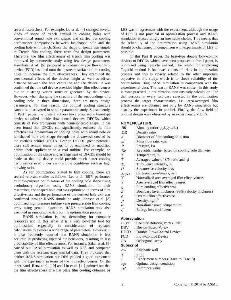
Figure 1 show the procedure of Taguchi method[12] [13].

Taguchi experiments are designed according to some strict rules.

Step (1) - (4) is carried out in order to design experiment. An

orthogonal array (OA) are used to design the experiment.

Commonly used OAs are available for 2, 3 and 4 level factors.

Therefore, Control factor of DFCD and noise factor of DFCD

were determined in step (1). Next, the level of each factor was

decided in step (2). In step (3) and (4), suitable OA is chosen

and each factor is assign to the OA. As for above-mentioned

step (1) - (4), details are shown in Section 2.3. In step (5), the

result of Taguchi experiment required for optimization (It is the

area averaged film effectiveness this time) is acquired based on

the designed experiment. The two result acquisition methods

(experimental and numerical method) were tried on this

research at the same time and under the same condition. Those

acquired result is shown in Section 5.1-5.3. The results of the

Taguchi experiments are analyzed in the step (6). In this step,

the factoral effects and optimal design are evaluated by

calculating the signal to noise (S/N) ratio. The optimum design

identified in the analysis should be tested to confirm that

performance indeed is the best and that it closely matches the

performance predicted by analysis (step (7)). Finally, these

experimentally- and numerically-optimal designs are compared

one-on-one. The detailed method of step(6) and (7) were shown

2.4.

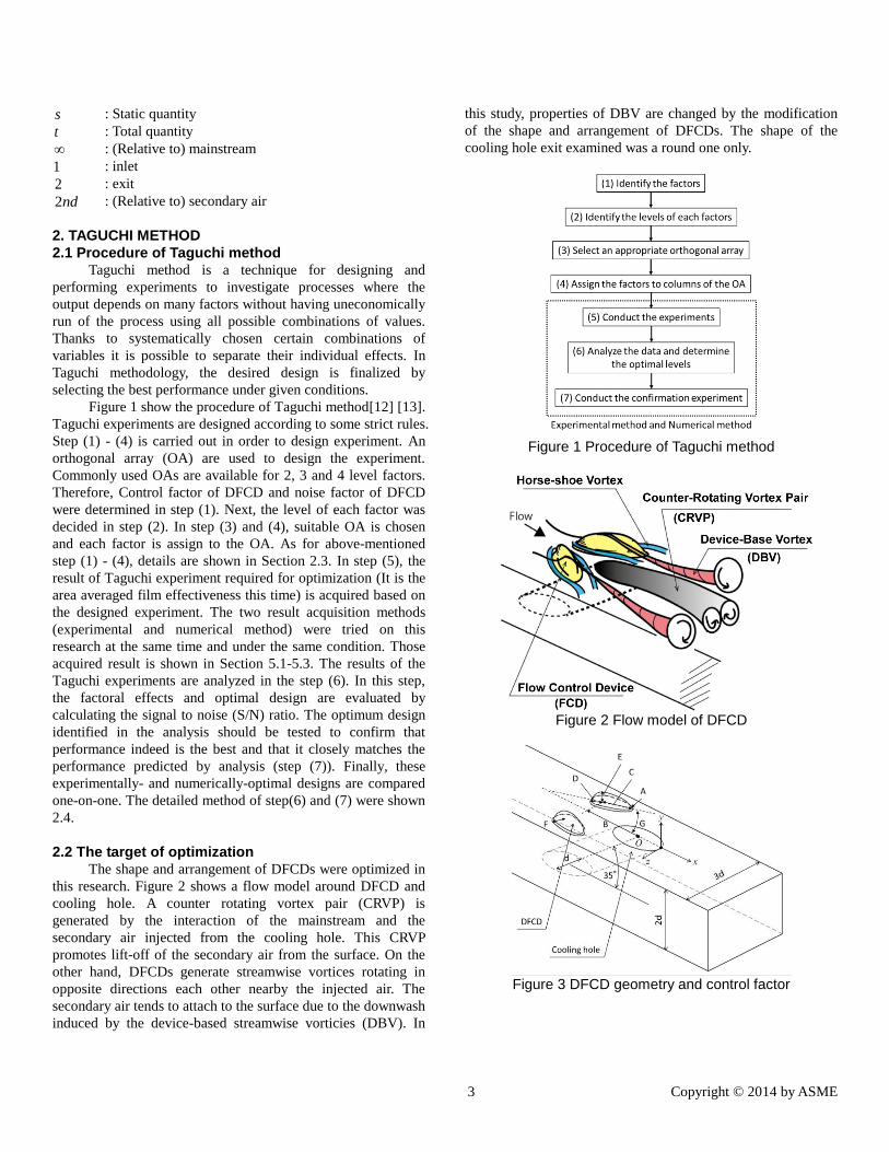
2.2 The target of optimization The shape and arrangement of DFCDs were optimized in

this research. Figure 2 shows a flow model around DFCD and

cooling hole. A counter rotating vortex pair (CRVP) is

generated by the interaction of the mainstream and the

secondary air injected from the cooling hole. This CRVP

promotes lift-off of the secondary air from the surface. On the

other hand, DFCDs generate streamwise vortices rotating in

opposite directions each other nearby the injected air. The

secondary air tends to attach to the surface due to the downwash

induced by the device-based streamwise vorticies (DBV). In

this study, properties of DBV are changed by the modification

of the shape and arrangement of DFCDs. The shape of the

cooling hole exit examined was a round one only.

Figure 1 Procedure of Taguchi method

Figure 2 Flow model of DFCD

Figure 3 DFCD geometry and control factor


2.3 Experiment design

2.3.1 Control factors

The outline view of cooling hole and DFCD geometry are

shown in Figure 3. The cooling hole used by this research was a

simple cylindrical cooling hole of 20mm diameter, d . The

inclination angle of the cooling hole was 35 degrees, the

thickness of the test model was 2 d and the hole pitch was 3d.

Two protrusive-type flow-control device (FCD) of hemi-

spheroid shape were attached to the surface with some

inclination angle to the main flow. The control factors

designated A to G, which were required for optimization, are

shown in the Figure 3. Descriptions on control factors appear in

Table 1. The allocated levels in each of the factors are indicated

in Table 2. Note that x , y and z axes are streamwise,

normal to the plate surface and lateral coordinates, respectively.

The origin of the coordinate system was on the trailing edge of

the hole exit. Two levels were allocated to the control factor A,

fillet radius of FCD. The lateral distance between two FCDs,

i.e., the length between the points on the base of FCD where its

peak appeared, was fixed at 1.5 d . This was for preventing two

FCDs from interfering each other or sticking out of one pitch

zone when the control factors changed. It was also based on the

same reason that the maximum of G was fixed at 15 degrees.

L18 was used as OA. Therefore, the 18 cases experiment was

conducted in this research. The factor level in each experiment

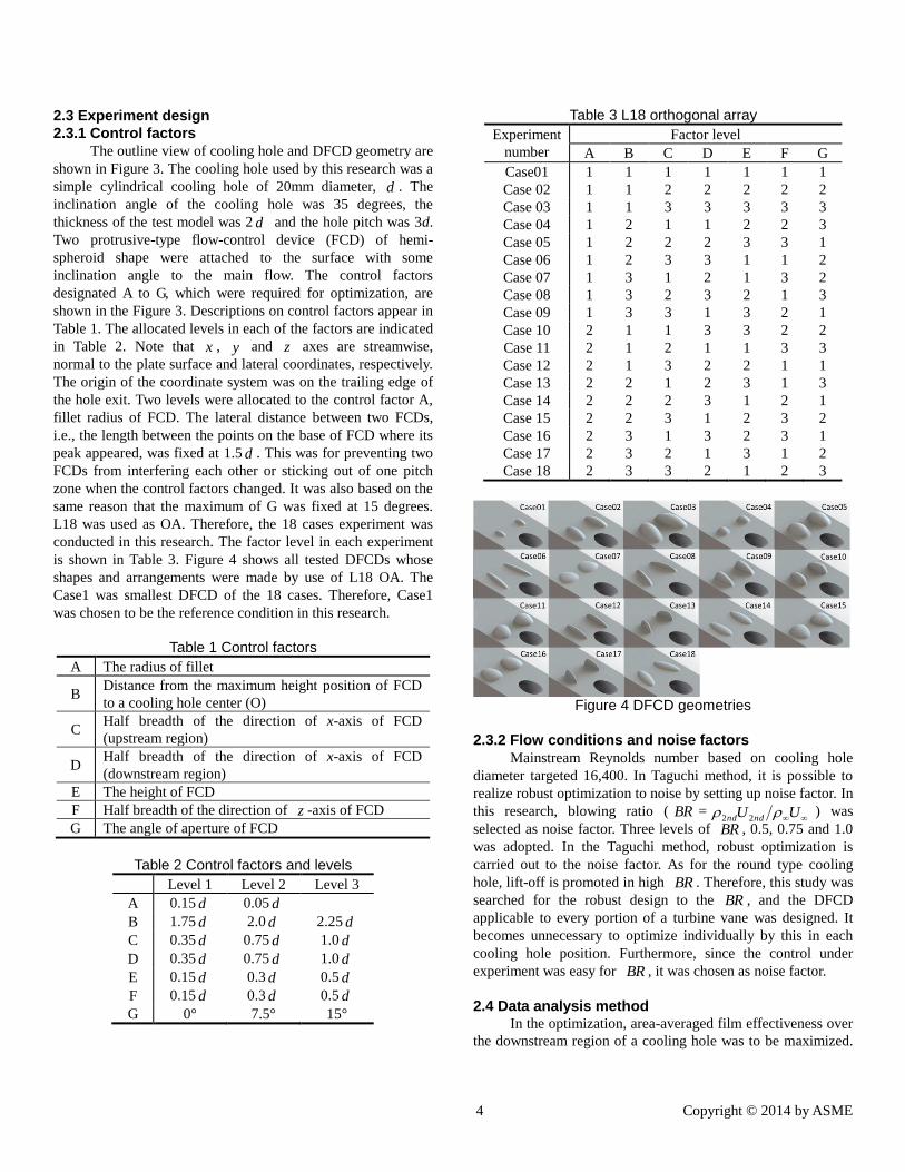
is shown in Table 3. Figure 4 shows all tested DFCDs whose

shapes and arrangements were made by use of L18 OA. The

Case1 was smallest DFCD of the 18 cases. Therefore, Case1

was chosen to be the reference condition in this research.

Table 1 Control factors

A The radius of fillet

B Distance from the maximum height position of FCD

to a cooling hole center (O)

C Half breadth of the direction of x-axis of FCD

(upstream region)

D Half breadth of the direction of x-axis of FCD

(downstream region)

E The height of FCD

F Half breadth of the direction of z -axis of FCD

G The angle of aperture of FCD

Table 2 Control factors and levels

Level 1 Level 2 Level 3

A 0.15 d 0.05 d

B 1.75 d 2.0 d 2.25 d

C 0.35 d 0.75 d 1.0 d

D 0.35 d 0.75 d 1.0 d

E 0.15 d 0.3 d 0.5 d

F 0.15 d 0.3 d 0.5 d

G 0° 7.5° 15°

Table 3 L18 orthogonal array

Experiment

number

Factor level

A B C D E F G

Case01 1 1 1 1 1 1 1

Case 02 1 1 2 2 2 2 2

Case 03 1 1 3 3 3 3 3

Case 04 1 2 1 1 2 2 3

Case 05 1 2 2 2 3 3 1

Case 06 1 2 3 3 1 1 2

Case 07 1 3 1 2 1 3 2

Case 08 1 3 2 3 2 1 3

Case 09 1 3 3 1 3 2 1

Case 10 2 1 1 3 3 2 2

Case 11 2 1 2 1 1 3 3

Case 12 2 1 3 2 2 1 1

Case 13 2 2 1 2 3 1 3

Case 14 2 2 2 3 1 2 1

Case 15 2 2 3 1 2 3 2

Case 16 2 3 1 3 2 3 1

Case 17 2 3 2 1 3 1 2

Case 18 2 3 3 2 1 2 3

Figure 4 DFCD geometries

2.3.2 Flow conditions and noise factors

Mainstream Reynolds number based on cooling hole

diameter targeted 16,400. In Taguchi method, it is possible to

realize robust optimization to noise by setting up noise factor. In

this research, blowing ratio ( BR =UU ndnd 22

) was

selected as noise factor. Three levels of BR , 0.5, 0.75 and 1.0

was adopted. In the Taguchi method, robust optimization is

carried out to the noise factor. As for the round type cooling

hole, lift-off is promoted in high BR . Therefore, this study was

searched for the robust design to the BR , and the DFCD

applicable to every portion of a turbine vane was designed. It

becomes unnecessary to optimize individually by this in each

cooling hole position. Furthermore, since the control under

experiment was easy for BR , it was chosen as noise factor.

2.4 Data analysis method In the optimization, area-averaged film effectiveness over

the downstream region of a cooling hole was to be maximized.


Therefore, “bigger is better” formulation (equation (1)) was

chosen in order to calculate a signal-to-noise (S/N) ratio, where

the signal means the film effectiveness and the noise was the

blowing ratio. The Y is the area averaged film effectiveness of

the region of 0 dx / 10 and -1.5 dz / 1.5. The i is

experiment number (Case1 to Case18). n is the number of noise

factor and n=3 in this study because BR was selected as noise

factor. Furthermore, Y of each case was normalized by Y of

the reference condition (Case1) of the same BR (equation(2)).

The overall film effectiveness in each case was defined by the

equation (3) using Y of each BR .

0.1,2

75.0,2

5.0,2

1111log10/

BRiBRiBRii

YYYnNS (1)

BRcase

BRi

BRiY

YY

,1

,

,

(2)

3

0.1,75.0,5.0,

BRiBRiBRi

i

YYY (3)

The area-averaged film effectiveness for calculating the

S/N ratio was acquired using the experimental and numerical

methods, from which two sets of optimal parameters were

determined. The detailed descriptions on the experimental and

numerical techniques are shown in the next chapter.

If we define the predicted S/N ratio and based on the

selected levels of the optimal design effects, the prediction

equation can be written as [12]:

)()()(

/,

TGTBTAT

NS

optoptopt

predictedpredicted

・・

(4)

T is the averaged value of S/N ratios or obtained in 18

trials based on the OA. As for each of the values of optA ,

optB , .. optG in equation (4), an averaged value of S/N ratios or

which are obtained in the trials including the optimal level is

used. For example, if A1 is the optimal level for factor A, A1 is

included in the trials from Case 1 to Case 9 according to the

OA, optA of

predicted is calculated by equation (5).

9

987654321 casecasecasecasecasecasecasecasecase

optA

(5)

3. EXPERIMENTAL RESULT ACQUISITION METHOD

3.1 Experimental Apparatus

The two different experimental setups of Iwate University

were employed, one for the aerothermal performance and the

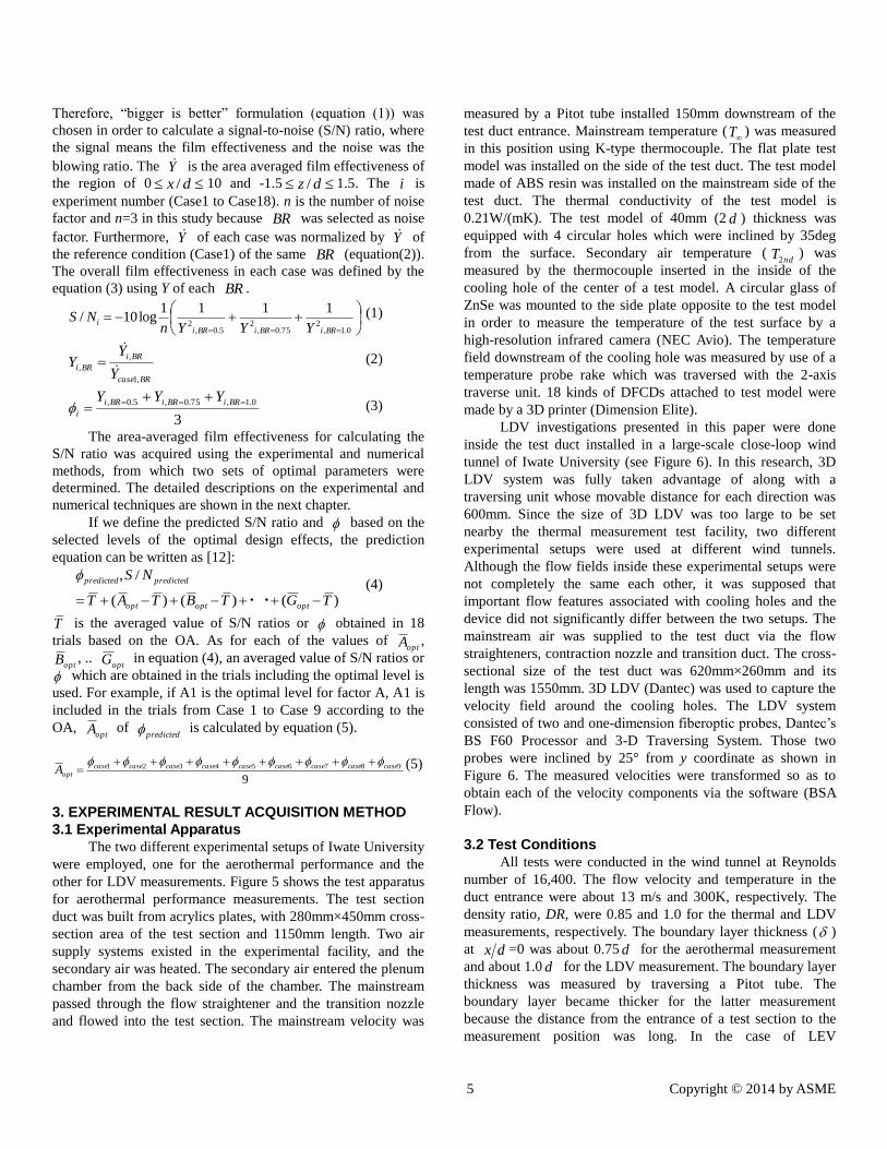
other for LDV measurements. Figure 5 shows the test apparatus

for aerothermal performance measurements. The test section

duct was built from acrylics plates, with 280mm×450mm cross-

section area of the test section and 1150mm length. Two air

supply systems existed in the experimental facility, and the

secondary air was heated. The secondary air entered the plenum

chamber from the back side of the chamber. The mainstream

passed through the flow straightener and the transition nozzle

and flowed into the test section. The mainstream velocity was

measured by a Pitot tube installed 150mm downstream of the

test duct entrance. Mainstream temperature (T ) was measured

in this position using K-type thermocouple. The flat plate test

model was installed on the side of the test duct. The test model

made of ABS resin was installed on the mainstream side of the

test duct. The thermal conductivity of the test model is

0.21W/(mK). The test model of 40mm (2 d ) thickness was

equipped with 4 circular holes which were inclined by 35deg

from the surface. Secondary air temperature (ndT2

) was

measured by the thermocouple inserted in the inside of the

cooling hole of the center of a test model. A circular glass of

ZnSe was mounted to the side plate opposite to the test model

in order to measure the temperature of the test surface by a

high-resolution infrared camera (NEC Avio). The temperature

field downstream of the cooling hole was measured by use of a

temperature probe rake which was traversed with the 2-axis

traverse unit. 18 kinds of DFCDs attached to test model were

made by a 3D printer (Dimension Elite).

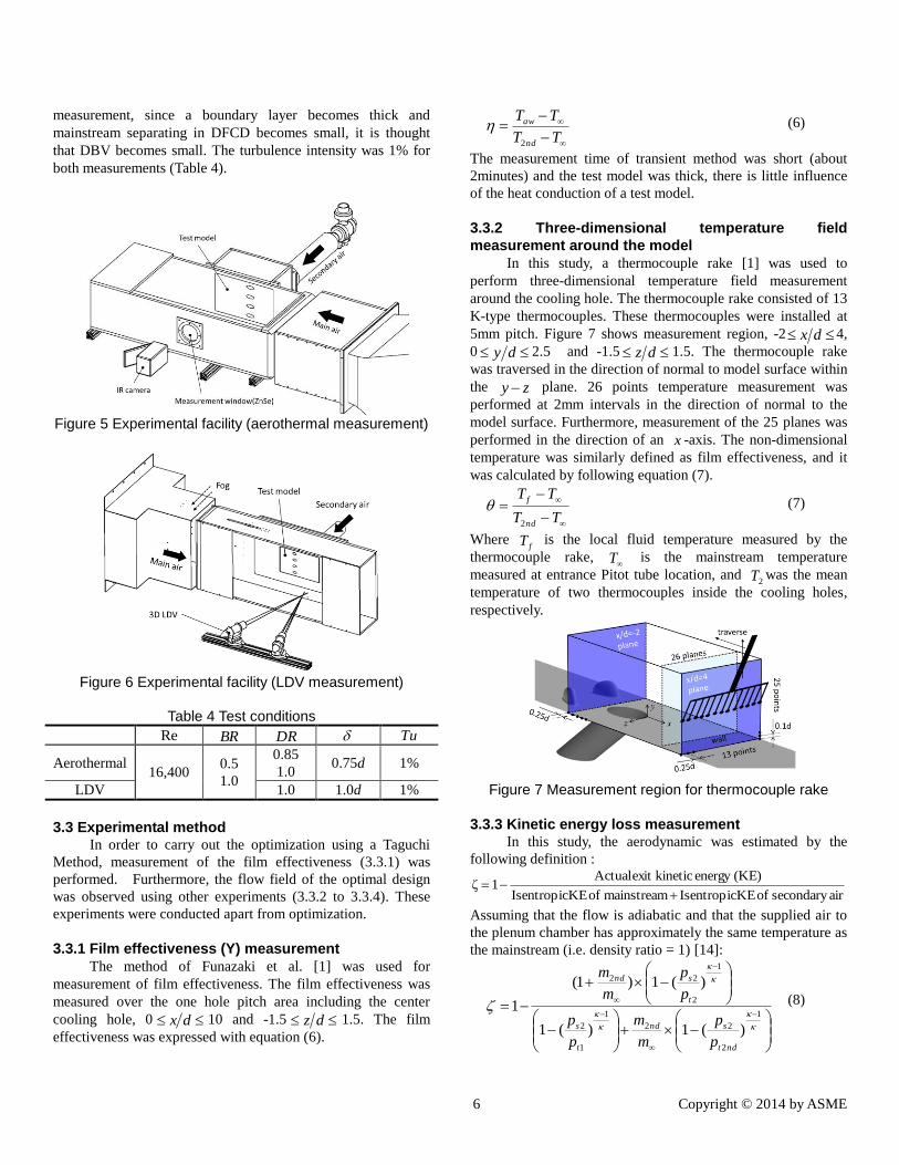
LDV investigations presented in this paper were done

inside the test duct installed in a large-scale close-loop wind

tunnel of Iwate University (see Figure 6). In this research, 3D

LDV system was fully taken advantage of along with a

traversing unit whose movable distance for each direction was

600mm. Since the size of 3D LDV was too large to be set

nearby the thermal measurement test facility, two different

experimental setups were used at different wind tunnels.

Although the flow fields inside these experimental setups were

not completely the same each other, it was supposed that

important flow features associated with cooling holes and the

device did not significantly differ between the two setups. The

mainstream air was supplied to the test duct via the flow

straighteners, contraction nozzle and transition duct. The cross-

sectional size of the test duct was 620mm×260mm and its

length was 1550mm. 3D LDV (Dantec) was used to capture the

velocity field around the cooling holes. The LDV system

consisted of two and one-dimension fiberoptic probes, Dantec’s

BS F60 Processor and 3-D Traversing System. Those two

probes were inclined by 25° from y coordinate as shown in

Figure 6. The measured velocities were transformed so as to

obtain each of the velocity components via the software (BSA

Flow).

3.2 Test Conditions

All tests were conducted in the wind tunnel at Reynolds

number of 16,400. The flow velocity and temperature in the

duct entrance were about 13 m/s and 300K, respectively. The

density ratio, DR, were 0.85 and 1.0 for the thermal and LDV

measurements, respectively. The boundary layer thickness ( )

at dx =0 was about 0.75 d for the aerothermal measurement

and about 1.0 d for the LDV measurement. The boundary layer

thickness was measured by traversing a Pitot tube. The

boundary layer became thicker for the latter measurement

because the distance from the entrance of a test section to the

measurement position was long. In the case of LEV


measurement, since a boundary layer becomes thick and

mainstream separating in DFCD becomes small, it is thought

that DBV becomes small. The turbulence intensity was 1% for

both measurements (Table 4).

Figure 5 Experimental facility (aerothermal measurement)

Figure 6 Experimental facility (LDV measurement)

Table 4 Test conditions

Re BR DR Tu

Aerothermal 16,400

0.5

1.0

0.85

1.0 0.75d 1%

LDV 1.0 1.0d 1%

3.3 Experimental method In order to carry out the optimization using a Taguchi

Method, measurement of the film effectiveness (3.3.1) was

performed. Furthermore, the flow field of the optimal design

was observed using other experiments (3.3.2 to 3.3.4). These

experiments were conducted apart from optimization.

3.3.1 Film effectiveness (Y) measurement

The method of Funazaki et al. [1] was used for

measurement of film effectiveness. The film effectiveness was

measured over the one hole pitch area including the center

cooling hole, 0 dx 10 and -1.5 dz 1.5. The film

effectiveness was expressed with equation (6).

TT

TT

nd

aw

2

(6)

The measurement time of transient method was short (about

2minutes) and the test model was thick, there is little influence

of the heat conduction of a test model.

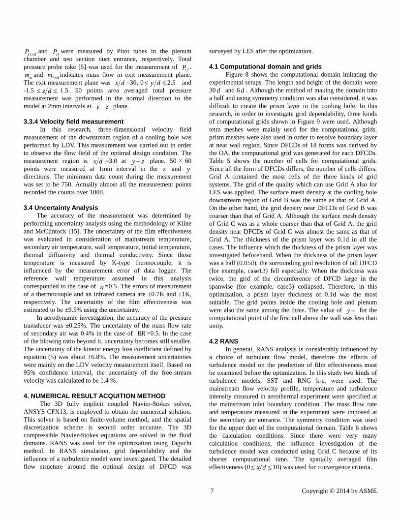
3.3.2 Three-dimensional temperature field

measurement around the model

In this study, a thermocouple rake [1] was used to

perform three-dimensional temperature field measurement

around the cooling hole. The thermocouple rake consisted of 13

K-type thermocouples. These thermocouples were installed at

5mm pitch. Figure 7 shows measurement region, -2 dx 4,

0 dy 2.5 and -1.5 dz 1.5. The thermocouple rake

was traversed in the direction of normal to model surface within

the zy plane. 26 points temperature measurement was

performed at 2mm intervals in the direction of normal to the

model surface. Furthermore, measurement of the 25 planes was

performed in the direction of an x -axis. The non-dimensional

temperature was similarly defined as film effectiveness, and it

was calculated by following equation (7).

TT

TT

nd

f

2

(7)

Where fT is the local fluid temperature measured by the

thermocouple rake, T is the mainstream temperature

measured at entrance Pitot tube location, and 2T was the mean

temperature of two thermocouples inside the cooling holes,

respectively.

Figure 7 Measurement region for thermocouple rake

3.3.3 Kinetic energy loss measurement In this study, the aerodynamic was estimated by the

following definition :

airsecondaryofKEIsentropicmainstreamofKEIsentropic

(KE)energykineticexitActual1ζ

Assuming that the flow is adiabatic and that the supplied air to

the plenum chamber has approximately the same temperature as

the mainstream (i.e. density ratio = 1) [14]:

1

2

22

1

1

2

1

2

22

)(1)(1

)(1)1(

1

ndt

snd

t

s

t

snd

p

p

m

m

p

p

p

p

m

m

(8)


ndtP2and

1tP were measured by Pitot tubes in the plenum

chamber and test section duct entrance, respectively. Total

pressure probe rake [5] was used for the measurement of 2tP .

m and ndm2

indicates mass flow in exit measurement plane.

The exit measurement plane was dx =30, 0 dy 2.5 and

-1.5 dz 1.5. 50 points area averaged total pressure

measurement was performed in the normal direction to the

model at 2mm intervals at zy plane.

3.3.4 Velocity field measurement

In this research, three-dimensional velocity field

measurement of the downstream region of a cooling hole was

performed by LDV. This measurement was carried out in order

to observe the flow field of the optimal design condition. The

measurement region is dx =3.0 at zy plane. 50× 60

points were measured at 1mm interval in the z and y

directions. The minimum data count during the measurement

was set to be 750. Actually almost all the measurement points

recorded the counts over 1000.

3.4 Uncertainty Analysis

The accuracy of the measurement was determined by

performing uncertainty analysis using the methodology of Kline

and McClintock [15]. The uncertainty of the film effectiveness

was evaluated in consideration of mainstream temperature,

secondary air temperature, wall temperature, initial temperature,

thermal diffusivity and thermal conductivity. Since those

temperature is measured by K-type thermocouple, it is

influenced by the measurement error of data logger. The

reference wall temperature assumed in this analysis

corresponded to the case of =0.5. The errors of measurement

of a thermocouple and an infrared camera are ±0.7K and ±1K,

respectively. The uncertainty of the film effectiveness was

estimated to be ±9.5% using the uncertainty.

In aerodynamic investigation, the accuracy of the pressure

transducer was ±0.25%. The uncertainty of the mass flow rate

of secondary air was 0.4% in the case of BR =0.5. In the case

of the blowing ratio beyond it, uncertainty becomes still smaller.

The uncertainty of the kinetic energy loss coefficient defined by

equation (5) was about ±6.8%. The measurement uncertainties

were mainly on the LDV velocity measurement itself. Based on

95% confidence interval, the uncertainty of the free-stream

velocity was calculated to be 1.4 %.

4. NUMERICAL RESULT ACQUITION METHOD

The 3D fully implicit coupled Navier-Stokes solver,

ANSYS CFX13, is employed to obtain the numerical solution.

This solver is based on finite-volume method, and the spatial

discretization scheme is second order accurate. The 3D

compressible Navier-Stokes equations are solved in the fluid

domains. RANS was used for the optimization using Taguchi

method. In RANS simulation, grid dependability and the

influence of a turbulence model were investigated. The detailed

flow structure around the optimal design of DFCD was

surveyed by LES after the optimization.

4.1 Computational domain and grids

Figure 8 shows the computational domain imitating the

experimental setups. The length and height of the domain were

30 d and 6 d . Although the method of making the domain into

a half and using symmetry condition was also considered, it was

difficult to create the prism layer in the cooling hole. In this

research, in order to investigate grid dependability, three kinds

of computational grids shown in Figure 9 were used. Although

tetra meshes were mainly used for the computational grids,

prism meshes were also used in order to resolve boundary layer

at near wall region. Since DFCDs of 18 forms was derived by

the OA, the computational grid was generated for each DFCDs.

Table 5 shows the number of cells for computational grids.

Since all the form of DFCDs differs, the number of cells differs.

Grid A contained the most cells of the three kinds of grid

systems. The grid of the quality which can use Grid A also for

LES was applied. The surface mesh density at the cooling hole

downstream region of Grid B was the same as that of Grid A.

On the other hand, the grid density near DFCDs of Grid B was

coarser than that of Grid A. Although the surface mesh density

of Grid C was as a whole coarser than that of Grid A, the grid

density near DFCDs of Grid C was almost the same as that of

Grid A. The thickness of the prism layer was 0.1d in all the

cases. The influence which the thickness of the prism layer was

investigated beforehand. When the thickness of the prism layer

was a half (0.05d), the surrounding grid resolution of tall DFCD

(for example, case13) fell especially. When the thickness was

twice, the grid of the circumference of DFCD large in the

spanwise (for example, case3) collapsed. Therefore, in this

optimization, a prism layer thickness of 0.1d was the most

suitable. The grid points inside the cooling hole and plenum

were also the same among the three. The value of y for the

computational point of the first cell above the wall was less than

unity.

4.2 RANS

In general, RANS analysis is considerably influenced by

a choice of turbulent flow model, therefore the effects of

turbulence model on the prediction of film effectiveness must

be examined before the optimization. In this study two kinds of

turbulence models, SST and RNG k-ε, were used. The

mainstream flow velocity profile, temperature and turbulence

intensity measured in aerothermal experiment were specified at

the mainstream inlet boundary condition. The mass flow rate

and temperature measured in the experiment were imposed at

the secondary air entrance. The symmetry condition was used

for the upper duct of the computational domain. Table 6 shows

the calculation conditions. Since there were very many

calculation conditions, the influence investigation of the

turbulence model was conducted using Grid C because of its

shorter computational time. The spatially averaged film

effectiveness (0 dx 10) was used for convergence criteria.


Figure 8 Computational domain

Figure 9 Computational grids

Table 5 Number of cells

Number of cells

Grid A About 8,000,000

Grid B About 6,800,000

Grid C About 5,000,000

Table 6 Calculation conditions

Turbulence model Computational grid

SST Grid A, Grid B and Grid C

RNG k-ε Grid C

4.3 LES

LES was used in order to investigate unsteady flow

structure inside the flow field with optimal DFCDs. Wall-

damping function was not used in this study. Dynamic

smagorinsky model was used for the SGS model. Central-

differencing scheme was used for advection scheme in LES. As

for the LES case, the non-dimensional time step was 3100.3

Ud . To obtain the time-averaged statistics the flow

field has been sampled over 3 time periods.

5. RESULT AND DISCUSSION

5.1 Analysis of experimental result

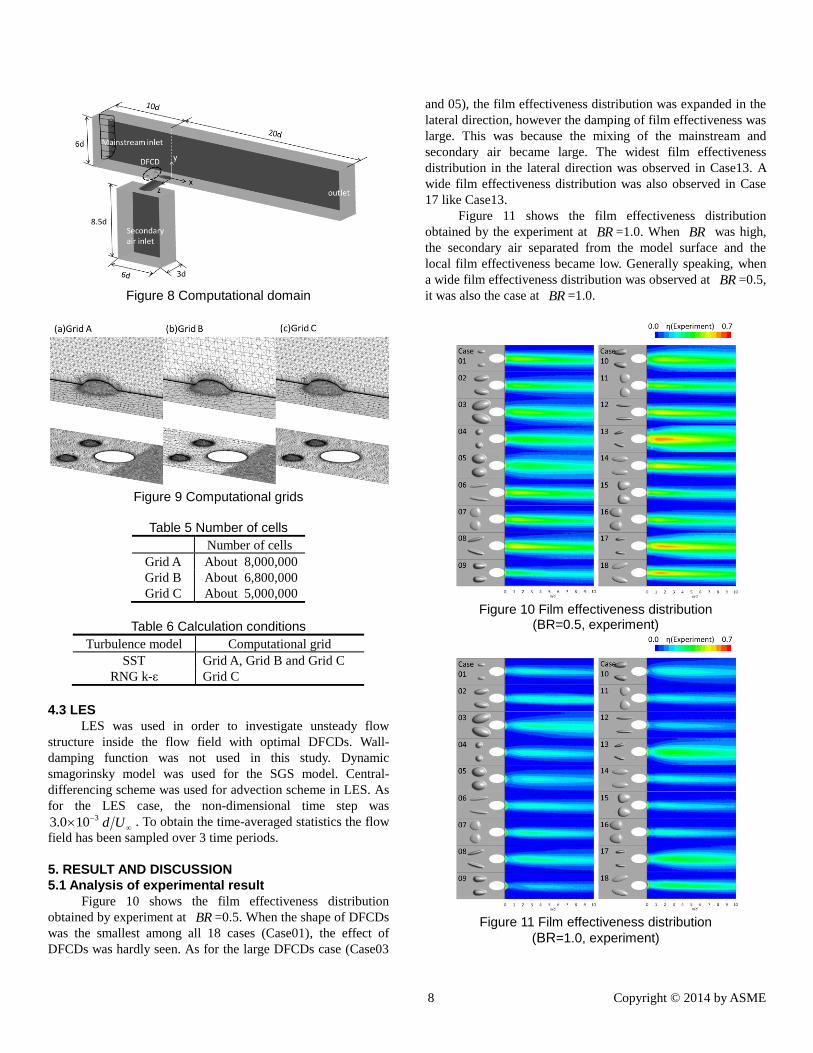
Figure 10 shows the film effectiveness distribution

obtained by experiment at BR =0.5. When the shape of DFCDs

was the smallest among all 18 cases (Case01), the effect of

DFCDs was hardly seen. As for the large DFCDs case (Case03

and 05), the film effectiveness distribution was expanded in the

lateral direction, however the damping of film effectiveness was

large. This was because the mixing of the mainstream and

secondary air became large. The widest film effectiveness

distribution in the lateral direction was observed in Case13. A

wide film effectiveness distribution was also observed in Case

17 like Case13.


obtained by the experiment at BR =1.0. When BR was high,

the secondary air separated from the model surface and the

local film effectiveness became low. Generally speaking, when

a wide film effectiveness distribution was observed at BR =0.5,

it was also the case at BR =1.0.

Figure 10 Film effectiveness distribution

(BR=0.5, experiment)


(BR=1.0, experiment)


Figure 12 shows the response graphs for major effects

obtained by the experimental result. The purpose of this

analysis was to find out factors that had strong effects on film

effectiveness. The error bar was described in consideration of

5.3% of the uncertainty of the area-averaged film effectiveness.

It was clear that factor E, F, and G had comparatively large

influences on the S/N ratio. Even if the uncertainties of E3 and

F1 were taken into consideration, the trend of their S/N ratio

levels to determine the maximum was unchanged. On the other

hand, factors A, B, C and D had comparatively little influence

on the S/N ratio. Since in Taguchi method optimal design set is

what makes each of the S/N ratios maximum, the selected

optimal design set was A2B2C1D2E3F1G3. As a result, the

predicted values of S/N ratio and were 8.86db and 2.57,

respectively.

In order to confirm the prediction, an experiment using

the optimal design was conducted. The S/N ratios and

which were obtained in the confirmation experiment were

7.87db and 2.52, respectively. The difference of the

confirmation value and the predicted value was less than ±3 db.

Therefore, sufficient repeatability was verified by this

experimental result.

Figure 12 Response graphs for major effects

(experiment)

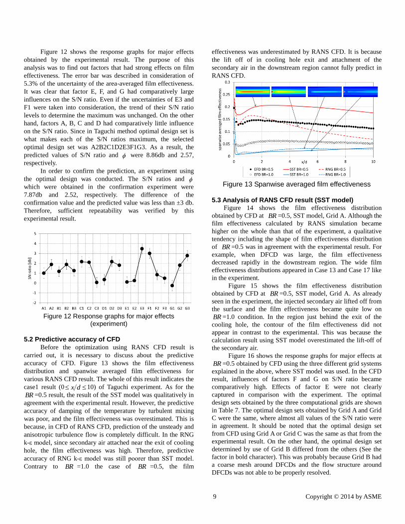
5.2 Predictive accuracy of CFD

Before the optimization using RANS CFD result is

carried out, it is necessary to discuss about the predictive

accuracy of CFD. Figure 13 shows the film effectiveness

distribution and spanwise averaged film effectiveness for

various RANS CFD result. The whole of this result indicates the

case1 result (0 dx 10) of Taguchi experiment. As for the

BR =0.5 result, the result of the SST model was qualitatively in

agreement with the experimental result. However, the predictive

accuracy of damping of the temperature by turbulent mixing

was poor, and the film effectiveness was overestimated. This is

because, in CFD of RANS CFD, prediction of the unsteady and

anisotropic turbulence flow is completely difficult. In the RNG

k-ε model, since secondary air attached near the exit of cooling

hole, the film effectiveness was high. Therefore, predictive

accuracy of RNG k-ε model was still poorer than SST model.

Contrary to BR =1.0 the case of BR =0.5, the film

effectiveness was underestimated by RANS CFD. It is because

the lift off of in cooling hole exit and attachment of the

secondary air in the downstream region cannot fully predict in

RANS CFD.

Figure 13 Spanwise averaged film effectiveness

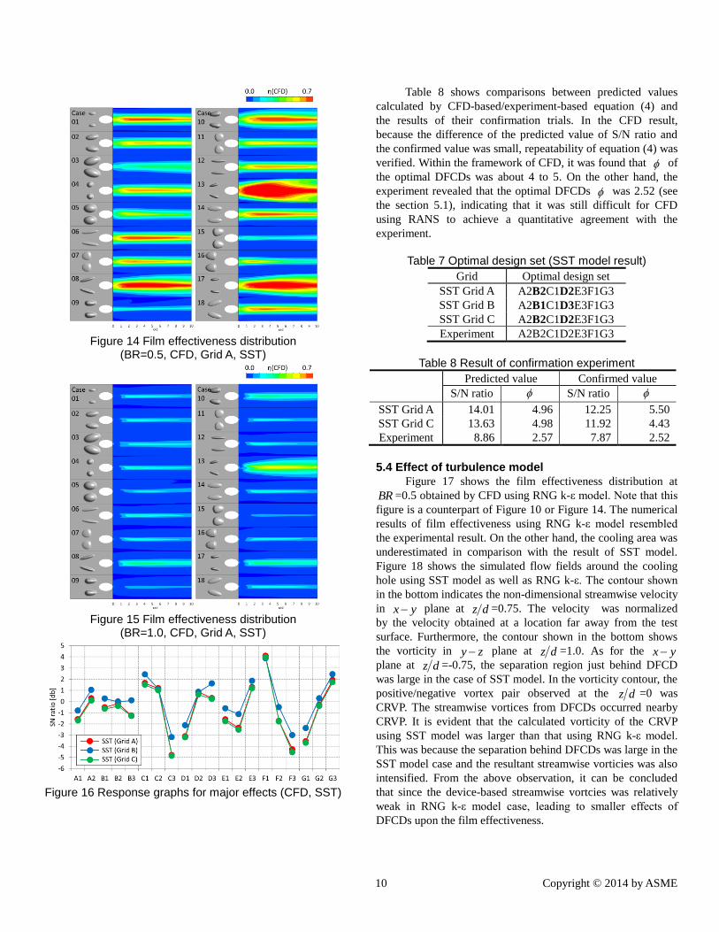
5.3 Analysis of RANS CFD result (SST model) Figure 14 shows the film effectiveness distribution

obtained by CFD at BR =0.5, SST model, Grid A. Although the

film effectiveness calculated by RANS simulation became

higher on the whole than that of the experiment, a qualitative

tendency including the shape of film effectiveness distribution

of BR =0.5 was in agreement with the experimental result. For

example, when DFCD was large, the film effectiveness

decreased rapidly in the downstream region. The wide film

effectiveness distributions appeared in Case 13 and Case 17 like

in the experiment.


obtained by CFD at BR =0.5, SST model, Grid A. As already

seen in the experiment, the injected secondary air lifted off from

the surface and the film effectiveness became quite low on

BR =1.0 condition. In the region just behind the exit of the

cooling hole, the contour of the film effectiveness did not

appear in contrast to the experimental. This was because the

calculation result using SST model overestimated the lift-off of

the secondary air.

Figure 16 shows the response graphs for major effects at

BR =0.5 obtained by CFD using the three different grid systems

explained in the above, where SST model was used. In the CFD

result, influences of factors F and G on S/N ratio became

comparatively high. Effects of factor E were not clearly

captured in comparison with the experiment. The optimal

design sets obtained by the three computational grids are shown

in Table 7. The optimal design sets obtained by Grid A and Grid

C were the same, where almost all values of the S/N ratio were

in agreement. It should be noted that the optimal design set

from CFD using Grid A or Grid C was the same as that from the

experimental result. On the other hand, the optimal design set

determined by use of Grid B differed from the others (See the

factor in bold character). This was probably because Grid B had

a coarse mesh around DFCDs and the flow structure around

DFCDs was not able to be properly resolved.



(BR=0.5, CFD, Grid A, SST)


(BR=1.0, CFD, Grid A, SST)

Figure 16 Response graphs for major effects (CFD, SST)

Table 8 shows comparisons between predicted values

calculated by CFD-based/experiment-based equation (4) and

the results of their confirmation trials. In the CFD result,

because the difference of the predicted value of S/N ratio and

the confirmed value was small, repeatability of equation (4) was

verified. Within the framework of CFD, it was found that of

the optimal DFCDs was about 4 to 5. On the other hand, the

experiment revealed that the optimal DFCDs was 2.52 (see

the section 5.1), indicating that it was still difficult for CFD

using RANS to achieve a quantitative agreement with the

experiment.

Table 7 Optimal design set (SST model result)

Grid Optimal design set

SST Grid A A2B2C1D2E3F1G3

SST Grid B A2B1C1D3E3F1G3

SST Grid C A2B2C1D2E3F1G3

Experiment A2B2C1D2E3F1G3

Table 8 Result of confirmation experiment

Predicted value Confirmed value

S/N ratio S/N ratio

SST Grid A 14.01 4.96 12.25 5.50

SST Grid C 13.63 4.98 11.92 4.43

Experiment 8.86 2.57 7.87 2.52

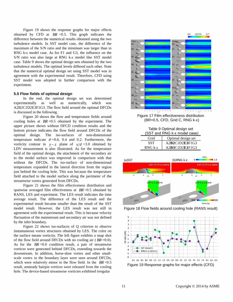
5.4 Effect of turbulence model

Figure 17 shows the film effectiveness distribution at

BR =0.5 obtained by CFD using RNG k-ε model. Note that this

figure is a counterpart of Figure 10 or Figure 14. The numerical

results of film effectiveness using RNG k-ε model resembled

the experimental result. On the other hand, the cooling area was

underestimated in comparison with the result of SST model.

Figure 18 shows the simulated flow fields around the cooling

hole using SST model as well as RNG k-ε. The contour shown

in the bottom indicates the non-dimensional streamwise velocity

in yx plane at dz =0.75. The velocity was normalized

by the velocity obtained at a location far away from the test

surface. Furthermore, the contour shown in the bottom shows

the vorticity in zy plane at dz =1.0. As for the yx

plane at dz =-0.75, the separation region just behind DFCD

was large in the case of SST model. In the vorticity contour, the

positive/negative vortex pair observed at the dz =0 was

CRVP. The streamwise vortices from DFCDs occurred nearby

CRVP. It is evident that the calculated vorticity of the CRVP

using SST model was larger than that using RNG k-ε model.

This was because the separation behind DFCDs was large in the

SST model case and the resultant streamwise vorticies was also

intensified. From the above observation, it can be concluded

that since the device-based streamwise vortcies was relatively

weak in RNG k-ε model case, leading to smaller effects of

DFCDs upon the film effectiveness.


Figure 19 shows the response graphs for major effects

obtained by CFD at BR =0.5. This graph indicates the

difference between the numerical results obtained using the two

turbulence models. In SST model case, the difference of the

maximum of the S/N ratio and the minimum was larger than in

RNG k-ε model case. As for F1 and G3, the influence on the

S/N ratio was also large at RNG k-ε model like SST model

case. Table 9 shows the optimal design sets obtained by the two

turbulence models. The optimal levels differed each other. Note

that the numerical optimal design set using SST model was in

agreement with the experimental result. Therefore, CFD using

SST model was adopted in further comparison with the

experiment.

5.5 Flow fields of optimal design

In the end, the optimal design set was determined

experimentally as well as numerically, which was

A2B2C1D2E3F1G3. The flow field around the optimal DFCDs

is discussed in the following.

Figure 20 shows the flow and temperature fields around

cooling holes at BR =0.5 obtained by the experiment. The

upper picture shows without DFCD condition results and the

bottom picture indicates the flow field around DFCDs of the

optimal design. The iso-surfaces of non-dimensional

temperature indicate =0.6, 0.4 and 0.2. Furthermore, the

vorticity contour in zy plane of dx =3.0 obtained by

LDV measurement is also illustrated. As for the temperature

field of the optimal design, the attachment of the secondary air

to the model surface was improved in comparison with that

without the DFCDs. The iso-surface of non-dimensional

temperature expanded in the lateral direction from the region

just behind the cooling hole. This was because the temperature

field attached to the model surface along the perimeter of the

streamwise vortex generated from DFCDs.

Figure 21 shows the film effectiveness distribution and

spanwise averaged film effectiveness at BR =0.5 obtained by

RANS, LES and experiment. The LES result indicates the time

average result. The difference of the LES result and the

experimental result became smaller than the result of the SST

model result. However, the LES result was not still in

agreement with the experimental result. This is because velocity

fluctuation of the mainstream and secondary air was not defined

by the inlet boundary.

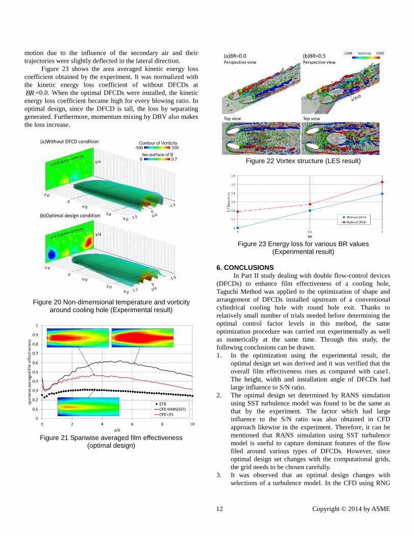
Figure 22 shows iso-surfaces of Q criterion to observe

instantaneous vortex structures obtained by LES. The color on

the surface means vorticity. The left figure exhibits a snap shot

of the flow field around DFCDs with no cooling air ( BR =0.0).

As for the BR =0.0 condition result, a pair of streamwise

vortices were generated behind DFCDs, extending towards the

downstream. In addition, horse-shoe vortex and other small-

scale vortex in the boundary layer were seen around DFCDs,

which were relatively minor in the flow field. In the BR =0.5

result, unsteady hairpin vortices were released from the cooling

hole. The device-based streamwise vorticies exhibited irregular


(BR=0.5, CFD, Grid C, RNG k-ε)

Table 9 Optimal design set (SST and RNG k-ε model case)

Grid Optimal design set

SST A2B2C1D2E3F1G3

RNG k-ε A2B3C1D2E1F1G3

Figure 18 Flow fields around cooling hole (RANS result)

Figure 19 Response graphs for major effects (CFD)


motion due to the influence of the secondary air and their

trajectories were slightly deflected in the lateral direction.

Figure 23 shows the area averaged kinetic energy loss

coefficient obtained by the experiment. It was normalized with

the kinetic energy loss coefficient of without DFCDs at

BR =0.0. When the optimal DFCDs were installed, the kinetic

energy loss coefficient became high for every blowing ratio. In

optimal design, since the DFCD is tall, the loss by separating

generated. Furthermore, momentum mixing by DBV also makes

the loss increase.

Figure 20 Non-dimensional temperature and vorticity

around cooling hole (Experimental result)

Figure 21 Spanwise averaged film effectiveness

(optimal design)

Figure 22 Vortex structure (LES result)

Figure 23 Energy loss for various BR values

(Experimental result)

6. CONCLUSIONS In Part II study dealing with double flow-control devices

(DFCDs) to enhance film effectiveness of a cooling hole,

Taguchi Method was applied to the optimization of shape and

arrangement of DFCDs installed upstream of a conventional

cylindrical cooling hole with round hole exit. Thanks to

relatively small number of trials needed before determining the

optimal control factor levels in this method, the same

optimization procedure was carried out experimentally as well

as numerically at the same time. Through this study, the

following conclusions can be drawn.

1. In the optimization using the experimental result, the

optimal design set was derived and it was verified that the

overall film effectiveness rises as compared with case1.

The height, width and installation angle of DFCDs had

large influence to S/N ratio.

2. The optimal design set determined by RANS simulation

using SST turbulence model was found to be the same as

that by the experiment. The factor which had large

influence to the S/N ratio was also obtained in CFD

approach likewise in the experiment. Therefore, it can be

mentioned that RANS simulation using SST turbulence

model is useful to capture dominant features of the flow

filed around various types of DFCDs. However, since

optimal design set changes with the computational grids,

the grid needs to be chosen carefully.

3. It was observed that an optimal design changes with

selections of a turbulence model. In the CFD using RNG


k-ε model, the optimal design set differed from that

determined by the experimental result. This was mainly

because the predictive accuracy of separation changed

with turbulence models.

4. In the optimal design obtained by the experimental result,

the device-based streamwise vorticies were observed in

the DFCD downstream region. These vortices appeared

nearby CRVP, sandwiching them. And the lift-off of

secondary air was suppressed. However, since the total

pressure loss measured in the downstream region

increased, optimization in consideration of aerodynamic

loss is required in the future.

ACKNOWLEDGMENTS This research and development has received funding for

advanced technology development for energy use

rationalization from the Electricity and Gas Industry

Department of the Agency for Natural Resources and Energy at

the Ministry of Economy, Trade and Industry. We would like to

express our thanks to the organizations.

REFERENCES [1] Funazaki, K., Nakata, R., Kawabata, H., Tagawa, H. and

Horiuchi, Y., 2014, “Improvement of Flat-Plate Film

Cooling Performance by Double Flow Control Devices:

Part I – Investigations on Capability of a Base-Type

Device”, ASME Turbo Expo 2014, GT2014- 25751.

[2] Barigozzi, G., Franchini, G., and Perdichizzi, A., 2007,

“The effect of an upstream ramp on cylindrical and fan-

shaped hole film cooling – part1: aerodynamic results”,

ASME Turbo Expo 2007, GT2007-27077.

[3] Barigozzi, G., Franchini, G., and Perdichizzi, A., 2007,

“The effect of an upstream ramp on cylindrical and fan-

shaped hole film cooling – part2: adiabatic effectiveness

results”, ASME Turbo Expo 2007, GT2007-27079.

[4] Lu, Y., Dhungel, A., Ekkad, S.V. and Bunker, R.S., 2008,

“Effect of trench width and depth on film cooling from

cylindrical holes embedded in trenches”, ASME Journal of

Turbomachinery., Vol.131, 011003.

[5] Kawabata, H., Funazaki, K., Nakata, R. and Takahashi, D.,

2013, “Experimental and Numerical Investigations of

Effect of Flow Control Devices upon Flat-Plate Film

Cooling Performance”, ASME Turbo Expo2013, GT2013-

95197.

[6] Lee, K.D. and Kim, K.Y., 2010, “Shape Optimization of a

Laidback Fan-Shaped Film-Cooling Hole to Enhance

Cooling Performance”, ASME Turbo Expo2010, GT2010-

22398.

[7] Lee, K.D., Kim, S.M. and Kim, K.Y., 2011, “Multi-

Objective Optimization of Film Cooling Holes

Considering Heat Transfer and Aerodynamic Loss”, ASME

Turbo Expo2011, GT2011-45402.

[8] Johnson, J.J., King, P.I., Clark, J.P. and Ooten, M.K.,

2013, “Genetic Algorithm Optimization of a High-

Pressure Turbine Vane Pressure Side Film Cooling Array”,

ASME Jornal of Turbomachinery., Vol.136, 011011.

[9] Sakai, E., Takahashi, T., Funazaki., K., Salleh, H.B. and

Watanabe, K., 2009, “Numerical Study on Flat Plate and

Leading Edge Film Cooling”, ASME Turbo Expo2009,

GT2009-59517.

[10] Renze, P. Schroder, M. and Meinke, M., 2008, “Large

eddy simulation of film cooling flows with variable

density jets”, Flow Turbulence Combust, 80, pp.119-132.

[11] Liu, K. and Pletcher, R.H., 2005, “Large Eddy Simulation

of Discrete-Hole Film Cooling in Flat Plate Turbulence

Bounday Layer”, 38th

AIAA Thermophysics Conference,

AIAA 2005-4944.

[12] Roy, R.K., 1990, “A Primer on the Taguchi Method”,

Society of Manufacturing Engineers Dearborn

[13] Chen, Y.H., Tam, S.C., Chen, W.L. and Zheng, H.Y., 1996,

“Application of Taguchi Method in The Optimization of

Laser Micro-Engraving of Photomasks”, International

Journal of Materials and Product Technology, Vol.11,

pp.333-344.

[14] Saha, R., Fridh, J., Fransson, T., Mamaev, B.I.,

Annerfeldt., 2013, “Suction and Pressure Side Film

Cooling Influence on Vane Aero Performance in a

Transonic Annular Cascade”, ASME Turbo Expo 2013,

GT2013-94319.

[15] Kline, S.J. and McClintock, F.A., 1953, “Describing

Uncertainties in Single Sample Experiments,” Mechanical

Engineering, Vol. 75, pp. 3-8.

improvement of flat-plate film cooling performance by

Documents