1

Improvement of Efficiency in a

Submersible Pump Motor

by

James Wall, BEng

This thesis is submitted as the fulfilment for the

requirement of the award of degree of

MASTER OF ENGINEERING (MEng)

by research from

DUBLIN CITY UNIVERSITY

Supervisor: Dr. Dermot Brabazon

2008

2

Dedication

I would like to dedicate this work to Mother and Father, My wife to be Ann and my

beloved son Taidgh - the source of all good in me.

3

Acknowledgments

I am to the highest degree thankful to my supervisor Dr. Dermot Brabazon, who has

always helped me in countless ways. He has always initiated challenging research ideas,

dedicated time, sourced out work opportunities that helped me financially and broadened

my aspects and expertise. On top of all, his humbleness and hands on personality have

always inspired me personally.

I very much thank Mr. Ben Breen, Technical Manager ABS, whose expertise in

various engineering fields facilitated the smooth running of this project and without his

backing would not have made this project possible. To Jean Noel Bajeet for his support and

expertise in CFD analysis.

4

Declaration

I hereby certify that this material, which I now submit for assessment on the programme of

study leading to the award of Master of Engineering is entirely my own work and has not

been taken from the work of others save and to the extent that such work has been cited

and acknowledged within the text of my own work.

Signed:_________________________ ID No.: 98036467

Date:____________

5

Abstract

The work covered in this project had the aim of improving the electrical efficiency of a

submersible pump. The requirement for the pump manufacturing industry to move in this

direction has increased recently with the introduction of new EU legislation making it a

requirement that new higher efficiency levels are met across the industry. In this work, the

use of the cooling jacket to keep the solenoid region of the pump cool was analysed and

improvements in design suggested. Specifically, the fluid flow and heat transfer in the

current pump cooling jacket was characterised. Improvement in the cooling jacket design

would give better heat transfer in the motor region of the pump and hence result in a higher

efficiency pump, with reduced induction resistance.

For this work, a dry pit installation pump testing system was added to the side of an already

existing 250 m3

test tank facility. This enabled high speed camera tracking of flow fields

and thermal imaging of the pump housing. The flow fields confirmed by CFD analysis

allowed alternate designs to be tried, tested and compared for maintaining as low an

operating temperature as possible. The original M60-4 pole pump design experienced a

maximum pump housing outside temperature of 45 C and a maximum stator temperature

of 90 C. A new cooling coil system investigated showed no improvement over the original

design. Increasing the number of impeller blades from four to eight reduced the running

temperature, measured on the housing, by seven degrees Celsius.

6

Table of Contents

Dedication

Acknowledgements

Declaration

Abstract

Chapter 1 Introduction

1.0 Historic Perspective 12

1.1 General Efficiency and Market Focus 12

1.2 Aims of the project 14

Chapter 2 Literature survey

2.1 Magnetism 15

2.2 Magnetic Propulsion within a Motor 15

2.3 AC Current 17

2.4 Basic AC Motor Operation 18

2.5 Power Factor 24

2.6 Motor Losses 24

2.6.1 Fixed Losses 26

2.6.2 Variable Losses 26

2.6.3 Eddy Currents 26

2.6.4 Stray Losses 27

2.7 Synchronous Speed 28

2.8 Life Cycle Cost Analysis 29

2.9 Stator Design 30

2.10 Rotor Design 31

2.11 Equivalent Circuit 31

2.12 Starting Characteristics 32

2.13 Running Characteristics 34

2.14 Motor Slip 36

2.15 Frame Classification 36

7

2.16 Temperature Classification 36

2.17 Cooling Systems 37

2.18 Numerical Simulation of the Cooling System 41

2.19 Review of Test Standards for Motor Efficiency 42

2.19.1International Electrotechnical Commission (IEC) 42

Chapter 3 Experimental/model set-up

3.1 Set-up for current closed cooling system analysis 43

3.1.1 Determination of temperatures generated by the induction motor 43

3.1.2 Determination of temperatures generated with cooling system 46

3.1.3 Determination of temperatures generated: coil cooling system 46

3.1.4 Examination of coolant flow around cooling jacket 48

3.1.5 Determination of flow rate from closed cooling impeller 49

3.1.6 Determination of power consumed by closed cooling system 49

3.2 Computational Fluid Dynamic (CFD) analysis 50

3.2.1 Set-up for CFD analysis 50

Chapter 4 Results

4.1 Introduction 53

4.1.1 Results of temperatures generated by the induction motor 53

4.1.2. Results of temperatures generated with cooling system 55

4.1.3 Results for temperatures generated with coil cooling system 57

4.1.4 Examination of coolant flow around the cooling jacket 59

4.1.5 Results for flow rate from closed cooling impeller 60

4.1.6 Results for power consumed by closed cooling system 60

4.2 Results from Computational Fluid Dynamic (CFD) analysis 61

4.3 Heat Transfer Calculations 65

4.3.1 No Cooling System 65

4.3.2 With Cooling System 66

4.3.3 With Coil Cooling System 68

4.3.4 Coil Cooling System with 4 Blade Impeller 69

8

Chapter 5 Conclusion and Recommendations

5.1 Conclusions 70

5.2 Recommendations for Future Work 71

References 73

Appendix A Performance of the closed cooling impeller 77

Appendix B Temperautres of the the bearing, water and phases 77

Appendix C Theraml image temperature profiles for coil cooling system 78

Appendix D Particle Speeds for Windows A1 to C3 79

Appendix E Fluid Velocity Through Inlet Pipe Using 8 Blade Impeller 84

Appendix F Fluid Velocity Through Inlet Pipe Using 4 Blade Impeller 84

Appendix G Schematics of Coil Cooling System 85

Appendix H Motor Performance curve 87

Appendix I Motor Test Standards 88

9

List of Figures

Figures of Chapter 1

Figure 1-1 Efficiency vs. load 13

Figures of Chapter 2

Figure 2-1 Magnetic fields in a simple electric motor 16

Figure 2-2 Example of a DC current time graph 17

Figure 2-3 Example of an AC current time graph 18

Figure 2-4 Basic elements of an electric motor 19

Figure 2-5 Rotating magnetic fields of the stator in a six pole motor 19

Figure 2-6 Three phase power supply current vs. time graph 21

Figure 2-7 Method of connecting three-phase power to a six-pole stator 21

Figure 2-8 Rotating magnetic field produced by a three-phase power supply 22

Figure 2-9 Construction of an AC induction motor’s rotor 23

Figure 2-10 Illustration of the current induced in the rotor 23

Figure 2-11 Picture of the location of losses typically found in an

AC submersible motor 28

Figure 2-12 Schematic of plan view of a pressed lamination 30

Figure 2-13 Typical torque – speed relationship for a synchronous motor 33

Figure 2-14 Cross section of closed cooling system 38

Figure 2-15 Schematic of heat flux driven by thermal conduction 40

Figures of Chapter 3

Figure 3-1 Picture of closed cooling experimental set-up with

submersible pump 43

Figure 3-2 Close up of heat exchange area 44

Figure 3-3 Position of thermocouple on motor housing 45

Figure 3-4 SolidWorks drawing of the coil cooling system 47

Figure 3-5 Top down view of housing location for windows A, B, C, and D 48

Figure 3-6 Pictures of Perspex windows A, B, C, and D, showing the

three zones examined for particle speeds 49

Figure 3-7 Flow chart indicting the steps used for model set-up 51

Figure 3-8 Screen shot of mated structures from ANSYS ICEM CFD 51

10

Figure 3-9 Meshed continuum of upper cooling jacket 52

Figures of Chapter 4

Figure 4-1 Housing temperature profiles recorded over a 3500 second

period at locations A, B, C, and D for operation without

a cooling system in place 54

Figure 4-2 Thermal image of the pump housing, taken after 1300 seconds,

without cooling system in place 54

Figure 4-3 Housing temperature profiles recorded over a 4000 second

period with a cooling system in place at locations A, B, C, D 55

Figure 4-4 Housing temperature profiles recorded over a 3720 second

period with a cooling system in place at locations on the

bearing, the three phase wirings, and the pumped water. 56

Figure 4-5 Thermal image of the pump housing, taken after 3500 seconds,

with the cooling system in operation. 56

Figure 4-6 Temperature rise in cooling system using standard 8 blade impeller 57

Figure 4-7 Thermal image of the pump housing, taken after 3000 seconds,

with the coil cooling system in operation 58

Figure 4-8 Temperature rise in cooling system using 4 blade impeller 58

Figure 4-9 Schematic of the flow field around cooling jacket 59

Figure 4-10 Graph of the power loss in the motor against the number

of motor poles 61

Figure 4-11 Screen shot of the CFD solution for the closed cooling system 62

Figure 4-12 Flow patterns around the cooling jacket as solved for in CFD 63

Figure 4-13 Screen shot showing pressure in Pa in the closed cooling system 64

Figure 4-14 Figure showing the radii and length of the stator region used

for the heat flow calculations. Note this is the cross sectional

side view plan view, the plan view of which is shown

in Figure 2-14 65

11

List of Tables

Table 2-1 Summary of losses in 2 and 4 pole motors 27

Table 2-2 Thermal Conductivity values of common materials 40

Table 4-1 Experimental settings and power consumed by open shaft

conditions with an without cooling impeller and seals.

(Voltage: 400V; Frequency: 50Hz). Note: the four pole motor

power here was higher than that used in this work; however the

trends of efficiency would be similar 60

12

Chapter 1 Introduction

1.0 Historic Perspective

In 1888 the induction motor was invented by Nikola Tesla, and by the mid 1890’s many

commercial designs were being manufactured. By the end of the first quarter of the 20th

century it was firmly established as the principle drive unit for plant and machinery

replacing water wheels and steam engines [1]. F.W. Pleuger invented the submersible

motor in 1929, which were then combined with slim centrifugal pumps during the

construction of the Berlin underground network to lower the water level during the

construction. An engineer by the name of Sixten Englesson invented the first submersible

drainage pump in 1947 and by 1956 had invented the first submersible sewage pump. After

this breakthrough, the submersible pumps were utilized in dewatering, water supply and

potable water distribution [2]. In the majority of industrial installations, electric motors

consume more than 60% of electricity produced with pump applications being more than

50% of this. The majority of motors are 3-phase induction motors and because of this large

usage today’s markets are increasingly concerned with efficiency.

1.1 General Efficiency and Market Focus

Due to environmental and economic pressures, today’s market is looking to conserve

energy. Potentially, increasing motor efficiency would cut the running cost of plants.

Motor design has, in general, been related to a market which was more concerned with the

initial cost of the motor, rather than the energy it consumed. High motor efficiency has

generally been only an incidental factor, with characteristics such as starting performance,

pull out torque and low noise level usually having higher priority as design criteria. The

motor size plays an important part, the larger the motor, generally the higher the efficiency.

Due to the size factor, efficiency improvement is more marked with the smaller size

motors. Generally within the range 1kW, higher motor efficiencies can be shown to

provide useful energy savings. Efficiency of a motor is calculated by dividing the

mechanically delivered shaft power Pmec by the total electrical input power Pel [3].

= Pmec /Pel

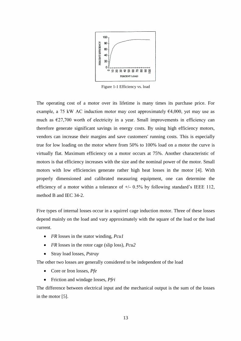
A typical curve of efficiency vs. load shows that efficiency increases according as the load

increases, see Figure 1.

13

Figure 1-1 Efficiency vs. load

The operating cost of a motor over its lifetime is many times its purchase price. For

example, a 75 kW AC induction motor may cost approximately €4,000, yet may use as

much as €27,700 worth of electricity in a year. Small improvements in efficiency can

therefore generate significant savings in energy costs. By using high efficiency motors,

vendors can increase their margins and save customers' running costs. This is especially

true for low loading on the motor where from 50% to 100% load on a motor the curve is

virtually flat. Maximum efficiency on a motor occurs at 75%. Another characteristic of

motors is that efficiency increases with the size and the nominal power of the motor. Small

motors with low efficiencies generate rather high heat losses in the motor [4]. With

properly dimensioned and calibrated measuring equipment, one can determine the

efficiency of a motor within a tolerance of +/- 0.5% by following standard’s IEEE 112,

method B and IEC 34-2.

Five types of internal losses occur in a squirrel cage induction motor. Three of these losses

depend mainly on the load and vary approximately with the square of the load or the load

current.

I²R losses in the stator winding, Pcu1

I²R losses in the rotor cage (slip loss), Pcu2

Stray load losses, Pstray

The other two losses are generally considered to be independent of the load

Core or Iron losses, Pfe

Friction and windage losses, Pfri

The difference between electrical input and the mechanical output is the sum of the losses

in the motor [5].

14

1.2 Aims of the project

The aims of this project are summarised in the following:

1- To understand the working principles of the pump and in particular the squirrel

cage induction motor, the sources of heat generation and the flow though the pump

cooling jacket for the submersible AFPKM60/4 pump.

2- To understand the efficiency standards, methods and procedure in determining the

efficiency of this asynchronous electric motor. To develop a finite volume model of

the current cooling system and examine its characteristics using CFD analysis.

3- To obtain experimental results to validate the results of the 3-D CFD model.

4- To develop a simple thermal model to examine the thermal field around the pump

housing.

5- To design and build a new cooling system and compare to current system.

6- Make suggestions for future design improvements.

15

Chapter 2 Literature survey

2.1 Magnetism

A permanent magnet will attract and hold metal objects when the object is near or in

contact with the magnet. The permanent magnet is able to do this because of its inherent

magnetic force, which is referred to as a "magnetic field".[7] Another but similar type of

magnetic field is produced around an electrical conductor when an electric current is

passed through a conductor. Lines of flux define the magnetic field and are in the form of

concentric circles around the wire. The "Left Hand Rule" rule states that if you point the

thumb of your left hand in the direction of the current, your fingers will point in the

direction of the magnetic field [8].

When a wire is shaped into a coil, all the individual flux lines produced by each section of

wire join together to form one large magnetic field around the coil. As with the permanent

magnet, these flux lines leave the north of the coil and re-enter the coil at its south pole.

The magnetic field of a wire coil is much greater and more localized than the magnetic

field around the plain conductor before being formed into a coil. Placing a core of iron or

similar metal in the center of the core can strengthen this magnetic field around the coil

even more. The metal core presents less resistance to the lines of flux than the air, thereby

causing the field strength to increase [9]. This is how a stator coil is made, a coil of wire

with a steel core. The advantage of a magnetic field that is produced by a current flowing

in a coil of wire is that when the current is reversed in direction the poles of the magnetic

field will switch positions since the lines of flux have changed direction. This phenomenon

is illustrated in Figure 2-1. Without this magnetic phenomenon existing, the AC motor as

we know it today would not exist.

2.2 Magnetic Propulsion within a Motor

The basic principle of all motors can easily be shown using two electromagnets and a

permanent magnet. Current is passed through a coil in such a direction that a north pole is

established and through a second coil in such a direction that a south pole is established. A

permanent magnet with a north and south pole, is the moving part of this simple motor

[10]. In Figure 2-1 step 1, the north pole of the permanent magnet is attracted towards the

16

south pole of the electromagnet. Similarly the south of the permanent magnet is attracted

towards the north pole of the electromagnet.

In Figure 2-1 step 2, the north and south poles are opposite each other. Like magnetic poles

repel each other, causing the movable permanent magnet to begin to turn. After it turns part

way around, the force of attraction between the unlike poles becomes strong enough to

keep the permanent magnet rotating. The rotating magnet continues to turn until the unlike

poles are lined up. At this point the rotor would normally stop because of the attraction

between the unlike poles.

Figure 2-1 Magnetic fields in a simple electric motor

If, however, the direction of currents in the electromagnetic coils were suddenly reversed,

thereby reversing the polarity of the two coils, then the poles would again be opposites and

repel each other. The movable permanent magnet would then continue to rotate. If the

current direction in the electromagnetic coils was changed every time the magnet turned

180 degrees or halfway around, then the magnet would continue to rotate. This simple

device is a motor in its simplest form. An actual motor is more complex than the simple

device shown above, but the principle is the same [11].

17

2.3 AC Current

The difference between DC and AC current is that with DC the current flows in only one

direction while with AC the direction of current flow changes periodically [12]. In the case

of 60Hz AC that is used throughout the US, the current flow changes direction 120 times

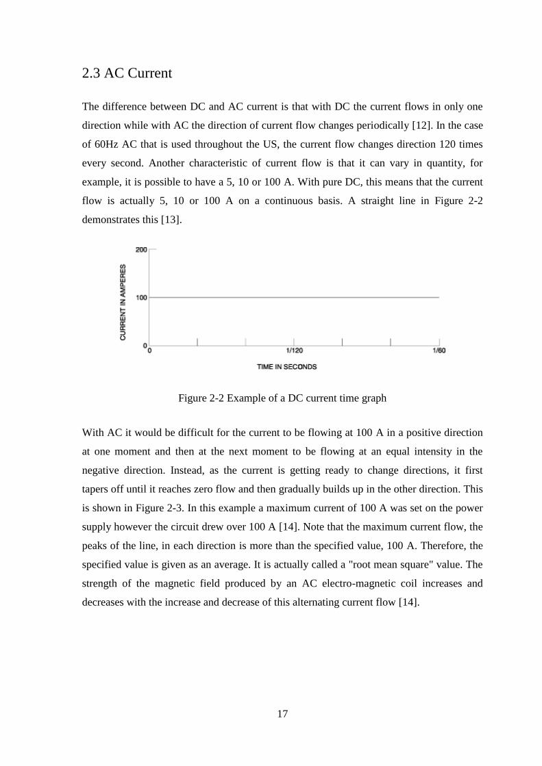
every second. Another characteristic of current flow is that it can vary in quantity, for

example, it is possible to have a 5, 10 or 100 A. With pure DC, this means that the current

flow is actually 5, 10 or 100 A on a continuous basis. A straight line in Figure 2-2

demonstrates this [13].

Figure 2-2 Example of a DC current time graph

With AC it would be difficult for the current to be flowing at 100 A in a positive direction

at one moment and then at the next moment to be flowing at an equal intensity in the

negative direction. Instead, as the current is getting ready to change directions, it first

tapers off until it reaches zero flow and then gradually builds up in the other direction. This

is shown in Figure 2-3. In this example a maximum current of 100 A was set on the power

supply however the circuit drew over 100 A [14]. Note that the maximum current flow, the

peaks of the line, in each direction is more than the specified value, 100 A. Therefore, the

specified value is given as an average. It is actually called a "root mean square" value. The

strength of the magnetic field produced by an AC electro-magnetic coil increases and

decreases with the increase and decrease of this alternating current flow [14].

18

Figure 2-3 Example of an AC current time graph

2.4 Basic AC Motor Operation

An AC motor has two basic electrical parts: a "stator" and a "rotor" as shown in Figure 2-4.

The stator is in the stationary electrical component. It consists of a group of individual

electro-magnets arranged in such a way that they form a hollow cylinder, with one pole of

each magnet facing toward the center of the group. The term, "stator" is derived from the

word stationary. The stator then is the stationary part of the motor [15]. The rotor is the

rotating electrical component. It also consists of a group of electro-magnets arranged

around a cylinder, with the poles facing toward the stator poles. The rotor, obviously, is

located inside the stator and is mounted on the motor's shaft. The term "rotor" is derived

from the word rotating. The rotor is the rotating part of the motor. The objective of these

motor components is to make the rotor rotate which in turn will rotate the motor shaft. This

rotation will occur because of the previously discussed magnetic phenomenon that unlike

magnetic poles attract each other and like poles repel. If we progressively change the

polarity of the stator poles in such a way that their combined magnetic field rotates, then

the rotor will follow and rotate with the magnetic field of the stator [16].

19

Figure 2-4 Basic elements of an electric motor

The rotating magnetic fields of a stator can be better understood by examining Figure 2-5.

As shown, the stator has six magnetic poles and the rotor has two poles. At time 1, stator

poles A-1 and C-2 are north poles and the opposite poles, A-2 and C-1, are south poles.

The S-pole of the rotor is attracted by the two N-poles of the stator and the two south poles

of the stator attract the N-pole of the rotor. At time 2, the polarity of the stator poles is

changed so that now C-2 and B-1 and N-poles and C-1 and B-2 are S-poles. The rotor then

is forced to rotate 60 degrees to line up with the stator poles as shown. At time 3, B-1 and

A-2 are N. At time 4, A-2 and C-1 are N. As each change is made, the poles of the rotor are

attracted by the opposite poles on the stator. As the magnetic field of the stator rotates, the

rotor is forced to rotate with it [17].

Figure 2-5 Rotating magnetic fields of the stator in a six pole motor

20

One way to produce a rotating magnetic field in the stator of an AC motor is to use a three-

phase power supply for the stator coils. Figure 2-6 depicts the current-time relation of

single-phase power [18]. The associated AC generator is producing just one flow of

electrical current whose direction and intensity varies as indicated by the single solid line

on the graph. From time 0 to time 3, current is flowing in the conductor in the positive

direction. From time 3 to time 6, current is flowing in the negative. At any one time, the

current is only flowing in one direction. Some generators produce three separate current

flows called phases all superimposed on the same circuit. This is referred to as three-phase

power. At any one instant, however, the direction and intensity of each separate current

flow are not the same as the other phases. This is illustrated in Figure 2-7. The three

separate phases are labeled A, B and C. At time 1, phase A is at zero amps, phase B is near

its maximum amperage and flowing in the positive direction, and phase C is near to its

maximum amperage but flowing in the negative direction. At time 2, the amperage of

phase A is increasing and flow is positive, the amperage of phase B is decreasing and its

flow is still negative, and phase C has dropped to zero amps. A complete cycle (from zero

to maximum in one direction, to zero and to maximum in the other direction, and back to

zero) takes one complete revolution of the generator. Therefore, a complete cycle, is said to

have 360 electrical degrees. From examining Figure2-10, we see that each phase is

displaced 120 degrees from the other two phases or 120 degrees out of phase [19].

To produce a rotating magnetic field in the stator of a three-phase AC motor the stator coils

need to be wound and the power supply leads connected [20]. The connection for a 6-pole

stator is shown in Figure 2-7. Each phase of the three-phase power supply is connected to

opposite poles and the associated coils are wound in the same direction. The polarity of the

poles of an electro-magnet are determined by the direction of the current flow through the

coil. Therefore, if two opposite stator electro-magnets are wound in the same direction, the

polarity of the facing poles must be opposite. Therefore, when pole A1 is N, pole A2 is S.

When pole B1 is N, B2 is S and so forth.

21

Figure 2-6 Three phase power supply current vs. time graph

Figure 2-7 Method of connecting three-phase power to a six-pole stator

Figure 2.8 shows how the rotating magnetic field is produced. At time 1, the current flow

in the phase "A" poles is positive and pole A-1 is N. The current flow in the phase "C"

poles is negative, making C-2 a N-pole and C-1 is S. There is no current flow in phase "B",

so these poles are not magnetized. At time 2, the phases have shifted 60 degrees, making

poles C-2 and B-1 both N and C-1 and B-2 both S. Thus, as the phases shift their current

22

flow, the resultant N and S poles move clockwise around the stator, producing a rotating

magnetic field. The rotor acts like a bar magnet, being pulled along by the rotating

magnetic field.

Figure 2-8 Rotating magnetic field produced by a three-phase power supply

Up to this point not much has been said about the rotor. In the previous examples, it has

been assumed the rotor poles were wound with coils, just as the stator poles, and supplied

with DC to create fixed polarity poles. This, by the way, is exactly how a synchronous AC

motor works. However, most AC motors being used today are not synchronous motors.

Instead, so-called "induction" motors are the workhorses of industry. So how is an

induction motor different? The big difference is the manner in which current is supplied to

the rotor. There is no external power supply. As you might imagine from the motor's name,

an induction technique is used instead [21]. Induction is another characteristic of

magnetism. It is a natural phenomena which occurs when a conductor, which are aluminum

bars in the case of a rotor, see Figure 2.9, is moved through an existing magnetic field or

when a magnetic field is moved past a conductor. In either case, the relative motion of the

two causes an electric current to flow in the conductor. This is referred to as "induced"

N S

23

current flow [22]. In other words, in an induction motor the current flow in the rotor is not

caused by any direct connection of the conductors to a voltage source, but rather by the

influence of the rotor conductors cutting across the lines of flux produced by the stator’s

magnetic fields. The induced current, which is produced in the rotor, results in a magnetic

field around the rotor conductors as shown in Figure 2.10. This magnetic field around each

rotor conductor will cause each rotor conductor to act like the permanent magnet in the

example shown. As the magnetic field of the stator rotates, due to the effect of the three-

phase AC power supply, the induced magnetic field of the rotor will be attracted and will

follow the rotation. The rotor is connected to the motor shaft, so the shaft will rotate and

drive the connection load [23].

Figure 2-9 Construction of an AC induction motor’s rotor

Figure 2-10 Illustration of the current induced in the rotor

24

2.5 Power Factor

Real power is defined as the ability of the circuit to perform work within a particular time.

Apparent power for a circuit is the product of the current and voltage measured in that

circuit. Power Factor is defined as the ratio of real power to apparent power. Power factor

is related to the phase angle between voltage and current when there is a clear linear

relationship. It can still be defined when there is no apparent phase relationship between

voltage and current, or when both voltage and current take on arbitrary values.

Power factor is a simple way to describe how much of the current contributes to real power

in the load. A power factor of one "unity power factor" is the goal of any electric utility

company and indicates that 100% of the current is contributing to power in the load. If the

power factor is less than one, they have to supply more current to the user for a given

amount of power use while a power factor of zero indicates that none of the current

contributes to power in the load. Purely resistive loads such as heater elements have a

power factor of unity. The current through them is directly proportional to the voltage

applied to them [40].

The current in an ac line can be thought of as consisting of two components: real and

imaginary. The real part results in power absorbed by the load while the imaginary part is

power being reflected back into the source, such as is the case when current and voltage are

of opposite polarity and their product, power, is negative. The reason it is important to have

a power factor as close as possible to unity is that once the power is delivered to the load,

we do not want any of it to be reflected back to the source. It took current to get the power

to the load and it will take current to carry it back to the source [41]. For more detail on

power factor correction in single phase motors and slip ring connections refer to Appendix

A.

2.6 Motor Losses

Induction motors have five major components of loss: iron loss, copper loss, frictional loss,

windage loss and sound loss. All these losses add up to the total loss of the induction

motor. Frictional loss, windage loss and sound losses are constant, independent of shaft

load, and are typically very small. The major losses are iron loss and copper loss. The iron

25

loss is essentially constant, independent of shaft load, while the copper loss is an I²R loss

which is shaft load dependent. The iron loss is voltage dependent and so will reduce with

reducing voltage. If we consider for example, an induction motor with a full load efficiency

of 90%, then we could expect that the iron loss is between 2.5% and 4% of the motor

rating. If by reducing the voltage, we are able to halve the iron loss, then this would equate

to an iron loss saving of 1-2% of the rated motor load. If the motor was operating under

open shaft condition, then the power consumed is primarily iron loss and we could expect

to achieve a saving of 30% - 60% of the energy consumed under normal working load shaft

conditions. It must be reiterated however, that this is a saving of only about 1-2% of the

rated motor load.

The current flowing into an induction motor comprises three major components,

magnetising current, loss current and load current. The magnetising current is essentially

constant, being dependent only on the applied voltage. The magnetising current is at phase

quadrate to the supply voltage and so does not contribute to any KW loading except for the

contribution to the copper loss of the motor. The magnetising current causes a reduction in

the power factor seen by the supply. The loss current is essentially a KW loading, as is the

load current. For a given shaft load, the output KW must remain constant [31]. As the

terminal voltage of the motor is reduced, the work current component must increase in

order to maintain the shaft output power (P = I x V). The increasing current resulting from

reducing voltage can in many instances result in an increasing I²R, which is in excess of

any iron loss reduction that may be achieved. For a large motor, the magnetising current

can be as low as 20% of the rated full load current of the motor. Three phase induction

motors have a high efficiency when operated at loads lower than 50% load. Experience

indicates that there is no large electrical cost saving by operating the motor well below

maximum rating.

Using silicon-controlled rectifiers (SCRs) to reduce the voltage applied to an induction

motor operating at reduced load and a high efficiency will reduce the iron loss, but there

will be an increase in current to provide the work output. This increase in current will

increase copper loss by the current squared, offsetting and often exceeding the reduction in

iron loss. This will often result in an increase in the total losses of the motor. The potential

to save energy with a solid state energy saving device, only becomes a reality when the

motor efficiency has fallen. This generally requires a considerable fall in power factor,

26

typically down to below 0.4 under full voltage operating conditions. Large motors have

lower iron loss (often 2 – 6% of the motor rating) and so the maximum achievable savings

are small relative to the motor rating. The losses found in any motor can be categorised

into fixed and variable losses.

2.6.1 Fixed Losses

The fixed losses as the name implies are virtually independent of the load on the motor or

when the motor is running on no load. They consist of friction losses in the bearings, also

air friction and turbulence around the rotor surface and core losses occurring in the core

steel, particularly in the stator. The core losses have two components, namely hysteresis

loss, representing the energy expended in reversing the direction of the flux, and the eddy

current losses caused by circulating currents within the core induced by the flux changes

[24].

2.6.2 Variable Losses

Variable losses or load losses are those arising from currents within the stator and rotor

conductors which are related to the load applied to the shaft, generally these losses can be

taken as varying as the square of the load I²R [25]. Variable losses can only be reduced

substantially by reducing the conductor resistances and this inevitably means larger

conductor cross-sectional areas. In turn this can result in a motor frame size increase,

which may also benefit the iron losses if flux densities are correspondingly reduced with

size [26].

2.6.3 Eddy Currents

An eddy current is a swirling current set up in a conductor in a response to a time-varying

magnetic field [27]. Since the motor housing material is resistive, ohmic power losses are

generated by the eddy current and appear as heat on the housing surface [28].

27

2.6.4 Stray Losses

All motors have stray losses due to a variety of causes and by careful design some of these

can be reduced for example the form and relative dimensions of the stator and rotor slots at

the air-gap surface. Using straight rotor slots as opposed to skewed rotor slots can also

reduce losses [29].

If all the above losses are reduced, then the heat to be removed from the motor is less, so

the coolant flow, which is often driven by an impeller in the close cooling system, can be

reduced with a further saving on fixed losses. AC motors typically feature rotors, which

consist of a laminated, cylindrical iron core with slots for receiving the conductors. The

most common type of rotor has cast-aluminum conductors and short-circuiting end rings.

This ac motor “squirrel cage” rotates when the moving magnetic field induces a current in

the shorted conductors. The speed at which the ac motor magnetic field rotates is the

synchronous speed of the ac motor and is determined by the number of poles in the stator

and the frequency of the power supply [30]:

ns = 120f / p,

where ns = synchronous speed, f = frequency, and p = the number of poles. Table 1 shows a

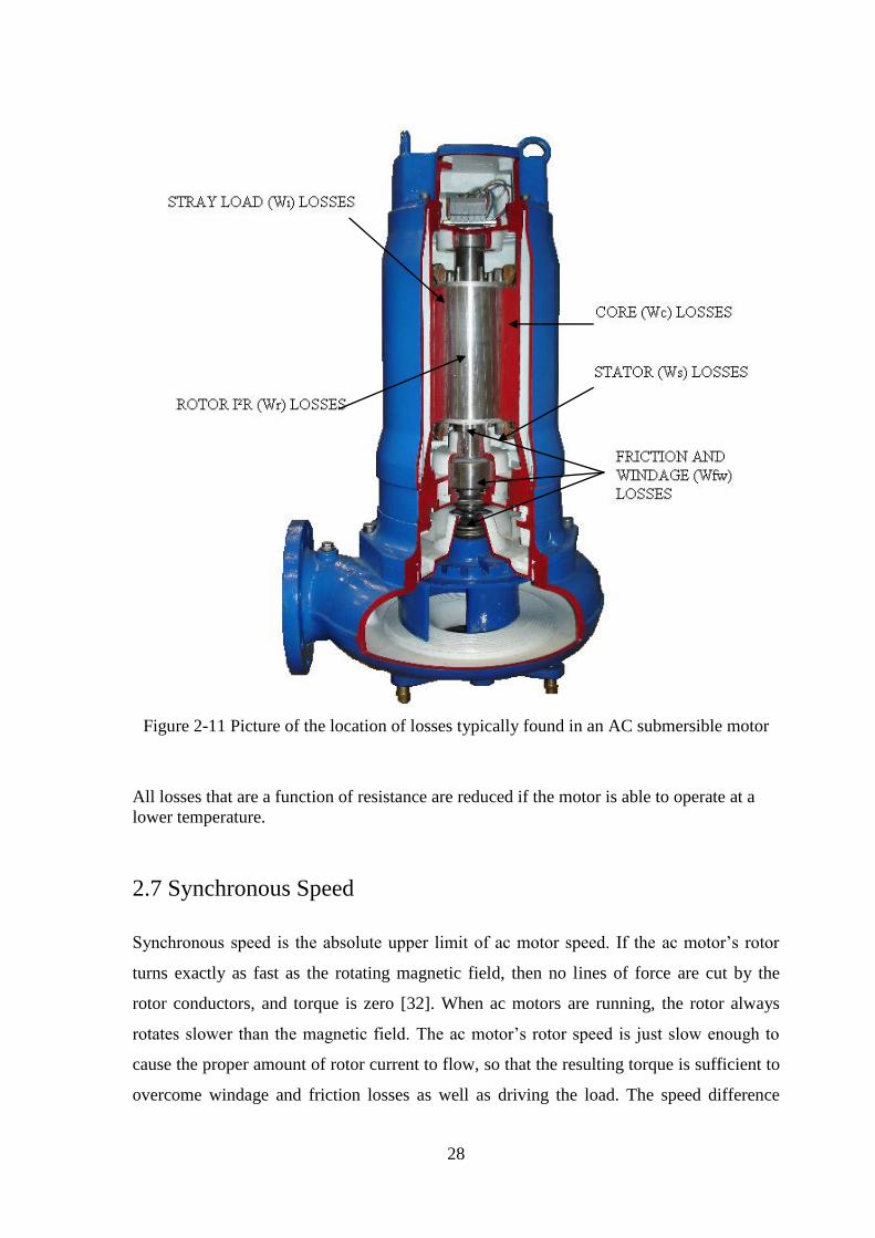
summary of the typical losses in a 2 and 4 pole motor. Figure 2.11 indicates the typical

location of losses.

Losses 2-Pole Average

4-Pole Average

Factors Affecting Losses

Core Losses Wc 19% 21% Electrical steel, saturation

Friction and Windage 25% 10% Closed cooling impeller,

Losses (Wfw) lubrication, bearings

Stator I²R Losses (Ws) 26% 34% Conductor area, mean length

of turn, heat dissipation

Rotor I²R Losses (Wr) 19% 21% Bar and end ring area and material

Stray I²R Losses (Wi) 11% 14% Manufacturing processes, slot

design, air gap

Table 2-1 Summary of losses in 2 and 4 pole motors

28

Figure 2-11 Picture of the location of losses typically found in an AC submersible motor

All losses that are a function of resistance are reduced if the motor is able to operate at a

lower temperature.

2.7 Synchronous Speed

Synchronous speed is the absolute upper limit of ac motor speed. If the ac motor’s rotor

turns exactly as fast as the rotating magnetic field, then no lines of force are cut by the

rotor conductors, and torque is zero [32]. When ac motors are running, the rotor always

rotates slower than the magnetic field. The ac motor’s rotor speed is just slow enough to

cause the proper amount of rotor current to flow, so that the resulting torque is sufficient to

overcome windage and friction losses as well as driving the load. The speed difference

29

between the ac motor’s rotor and magnetic field, called slip, is normally referred to as a

percentage of synchronous speed [33]:

s = 100 (ns – na)/ns,

where s = slip, ns = synchronous speed, and na = actual speed.

2.8 Life Cycle Cost Analysis

As stated in Chapter 1, 30 percent of electricity consumed in the world today is by pumps.

As a result of this high usage many municipal and industrial users are now focusing on the

life cycle Cost (LCC) analysis. As defined in the handbook by Europump and the

Hydraulic Institute, this is given by:

LCC = Cic + Cin +Ce + Co + Cm + Cs +Cenv + Cd

where: Cic is the initial cost of the equipment; Cin is the installation cost, commissioning

and training; Ce is the energy costs (including efficiency losses); Co is the operational

costs (normal operational/supervisory labour); Cm is the maintenance and repair cost; Cs is

the downtime cost (loss of production); Cenv is the environmental cost (contamination

from pumped liquid and auxiliary equipment); and Cd is the decommissioning cost.

When evaluating the total costs of a pumping system, it is important to consider all of the

above LCC analysis components before making a final decision. Other pump equipment

may offer low initial cost but offer very poor efficiency and thus making energy costs more

expensive than would be with the case of a higher efficiency piece of equipment [34]. It is

important, therefore, to consider both purchase price and operational costs when

purchasing equipment to properly account for the true overall cost of the equipment. A

deeper analysis of the operational efficiency details provides a more in depth view of the

“real life” issues that exist in today’s water and wastewater applications [35].

30

2.9 Stator Design

The stator is the outer body of the motor which houses the driven windings on an iron core.

In a single speed three phase motor design, the standard stator has three windings, while a

single phase motor typically has two windings. The stator core is made up of a stack of

round pre-punched laminations pressed into a frame which may be made of aluminium or

cast iron, see Figure 2-14. The laminations are basically round with a round hole inside

through which the rotor is positioned. The inner surface of the stator is made up of a

number of deep slots or grooves right around the stator. It is into these slots that the

windings are positioned. The arrangement of the windings or coils within the stator

determines the number of poles that the motor has [36]. A standard bar magnet has two

poles, generally known as North and South. Likewise, an electromagnet also has a North

and a South pole. As the induction motor stator is essentially like one or more

electromagnets depending on the stator windings, it also has poles in multiples of two e.g.

2 pole, 4 pole, 6 pole etc.

The winding configuration, slot configuration and lamination steel all have an effect on the

performance of the motor. The voltage rating of the motor is determined by the number of

turns on the stator and the power rating of the motor is determined by the losses which

comprise copper loss and iron loss, and the ability of the motor to dissipate the heat

generated by these losses. By introducing a larger wire gauge into the stator, this can

reduce the stator winding losses due to reduced resistance to current flow [37]. The stator

design determines the rated speed of the motor and largely other full load and full speed

characteristics such as power rating, current consumption and efficiency.

Figure 2-12 Schematic of plan view of a pressed lamination.

31

2.10 Rotor Design

The rotor comprises of a cylinder made up of round laminations pressed onto the motor

shaft, and a number of short-circuited windings. The rotor windings are made up of rotor

bars passed through the rotor, from one end to the other, around the surface of the rotor.

The bars protrude beyond the rotor and are connected together by a shorting ring at each

end. The bars are usually made of aluminium or copper, but sometimes made of brass. The

position of the bars relative to the surface of the rotor, as well as their shape, cross

sectional area and material determine the rotor characteristics. Essentially, the rotor bars

exhibit inductance and resistance, and these characteristics can effectively be dependant on

the frequency of the current flowing in the rotor. A bar with a large cross sectional area

will exhibit a low resistance, while a bar of a small cross sectional area will exhibit a high

resistance. Likewise a copper bar will have a low resistance compared to a brass or

aluminium bar of equal proportions.

Positioning the bar deeper into the rotor, increases the amount of iron around the bar, and

consequently increases the inductance exhibited by the rotor. The impedance of the bar is

made up of both resistance and inductance, and so two bars of equal dimensions will

exhibit different ac impedance depending on their position relative to the surface of the

rotor. A thin bar which is inserted radially into the rotor, with one edge near the surface of

the rotor and the other edge towards the shaft, will effectively change in resistance as the

frequency of the current changes. This is because the ac impedance of the outer portion of

the bar is lower than the inner impedance at high frequencies lifting the effective

impedance of the bar relative to the impedance of the bar at low frequencies where the

impedance of both edges of the bar will be lower and almost equal. The rotor design

determines the starting characteristics [38].

2.11 Equivalent Circuit

The induction motor can be treated essentially as a transformer for analysis. The induction

motor has stator leakage reactance, stator copper loss elements as series components, and

iron loss and magnetising inductance as shunt elements. The rotor circuit likewise has rotor

leakage reactance, rotor copper (aluminium) loss and shaft power as series elements. The

32

transformer in the centre of the equivalent circuit can be eliminated by adjusting the values

of the rotor components in accordance with the effective turn’s ratio of the transformer.

From the equivalent circuit and a basic knowledge of the operation of the induction motor,

it can be seen that the magnetising current component and the iron loss of the motor are

voltage dependant, and not load dependant. Additionally, the full voltage starting current of

a particular motor is voltage and speed dependant, but not load dependant. The

magnetising current varies depending on the design of the motor. For small motors, the

magnetising current may be as high as 60%, but for large two pole motors, the magnetising

current is more typically 20 – 25%. At the design voltage, the iron is typically near

saturation, so the iron loss and magnetising currents do not vary linearly with voltage as

saturation is approached. Within this operation region, small increases in voltage result in a

high increase in magnetising current and iron loss [39].

2.12 Starting Characteristics

In order to perform useful work, the induction motor must be started from rest and both the

motor and load accelerated up to full speed. Typically, this is done by relying on the high

slip characteristics of the motor and enabling it to provide the acceleration torque [42].

Induction motors at rest, appear just like a short circuited transformer, and if connected to

the full supply voltage, draw a very high current known as the “Locked Rotor Current”.

They also produce torque which is known as the “Locked Rotor Torque” LRT. The LRT

and the LRC are a function of the terminal voltage to the motor, and the motor design. As

the motor accelerates, both the torque and the current will tend to alter with rotor speed if

the voltage is maintained constant, see Figure 2-13.

The starting current of a motor, with a fixed voltage, will drop very slowly as the motor

accelerates and will only begin to fall significantly when the motor has reached at least

80% full speed. The actual curves for induction motors can vary considerably between

designs, but the general trend is for a high current until the motor has almost reached full

speed. The LRC of a motor can range from 500% Full Load Current (FLC) to as high as

1400% FLC. Typically, good motors fall in the range of 550% to 750% FLC [43]. The

starting torque of an induction motor starting with a fixed voltage, will drop a little to the

minimum torque known as the pull up torque as the motor accelerates, and then rise to a

33

maximum torque known as the breakdown or pull out torque at almost full speed and then

drop to zero at synchronous speed. The curve of start torque against rotor speed is

dependant on the terminal voltage and the motor/rotor design.

Figure 2-13 Typical torque – speed relationship for a synchronous motor

The LRT of an induction motor can vary from as low as 60% Full Load Torque (FLT) to as

high as 350% FLT. The pull-up torque can be as low as 40% FLT and the breakdown

torque can be as high as 350% FLT. Typical LRT’s for medium to large motors are in the

order of 120% FLT to 280% FLT [44]. The power factor of the motor at start is typically

0.1 – 0.25, rising to a maximum as the motor accelerates, and then falling again as the

motor approaches full speed. A motor which exhibits a high starting current, for example

850% of normal full load current, will generally produce a low starting torque, whereas a

motor which exhibits a low starting current will usually produce a high starting torque.

This is the reverse of what is generally expected.

The induction motor operates due to the torque developed by the interaction of the stator

field and the rotor field. Both of these fields are due to currents which have resistive or in

phase components and reactive or out of phase components. The torque developed is

dependant on the interaction of the in phase components and consequently is related to the

power consumed, I2R, within the rotor. A low rotor resistance will result in the current

being controlled by the inductive component of the circuit, yielding a high out of phase

current and a low torque [45].

34

Figures for the LRC and LRT are almost always quoted in motor data, and certainly are

readily available for induction motors. Some manufactures have been known to include

this information on the motor name plate. One additional parameter which would be of

tremendous use in data sheets for those who are developing motors for starting

applications, is the starting efficiency of the motor. The starting efficiency of the motor

refers to the ability of the motor to convert Amps into Newton-meters. This is a concept

not generally recognised within the trade, but one which is extremely useful when

comparing induction motors. The easiest means of developing a meaningful figure of merit

is to take the LRT of the motor (as a percentage of the full load torque) and divide it by the

LRC of the motor (as a percentage of the full load current) [46].

If the terminal voltage to the motor is reduced while it is starting, the current drawn by the

motor will be reduced proportionally. The torque developed by the motor is proportional to

the current squared, and so a reduction in starting voltage will result in a reduction in

starting current and a greater reduction in starting torque. If the start voltage applied to a

motor is halved, the start torque will be reduced by a quarter, likewise a start voltage of one

third nominal value will result in a start torque reduced by one ninth.

2.13 Running Characteristics

Once the motor is up to speed, it operates at low slip, at a speed determined by the number

of stator poles. The frequency of the current flowing in the rotor is very low. Typically, the

full load slip for a standard cage induction motor is less than 5%. The actual full load slip

of a particular motor is dependant on the motor design with typical full load speeds of four

pole induction motor varying between 1420 and 1480 RPM at 50 Hz. The synchronous

speed of a four pole machine at 50 Hz is 1500 RPM and at 60 Hz a four pole machine has a

synchronous speed of 1800 RPM [47].

The induction motor draws a magnetising current while it is operating. The magnetising

current is independent of the load on the machine, but is dependant on the design of the

stator and the stator voltage. The actual magnetising current of an induction motor can vary

from as low as 20% FLC for large two pole motors to as high as 60% for small eight pole

motors. The tendency is for large motors and high-speed motors to exhibit a low

35

magnetising current, while low speed motors and small motors exhibit a high magnetising

current. A typical medium sized four pole motor has a magnetising current of about 33%

FLC [48].

A low magnetising current indicates a low iron loss, while a high magnetising current

indicates an increase in iron loss and a resultant reduction in operating efficiency.

The resistive component of the current drawn by the motor while operating, changes with

load, being primarily load current with a small current for losses. If the motor is operated at

minimum load, i.e. open shaft, the current drawn by the motor is primarily magnetising

current and is almost purely inductive. Being an inductive current, the power factor is very

low, typically as low as 0.1. As the shaft load on the motor is increased, the resistive

component of the current begins to rise. The average current will noticeably begin to rise

when the load current approaches the magnetising current in magnitude. As the load

current increases, the magnetising current remains the same and so the power factor of the

motor will improve. The full load power factor of an induction motor can vary from 0.5 for

a small low speed motor up to 0.9 for a large high speed machine [49].

The losses of an induction motor comprise: iron loss, copper loss, windage loss and

frictional loss. The iron loss, windage loss and frictional losses are all essentially load

independent, but the copper loss is proportional to the square of the stator current.

Typically the efficiency of an induction motor is highest at 3/4 load and varies from less

than 60% for small low speed motors to greater than 92% for large high speed motors.

Operating power factor and efficiencies are generally quoted on the motor data sheets [50].

2.14 Motor Slip

There must be a relative difference in speed between the rotor and the rotating magnetic

field. If the rotor and the rotating magnetic field were turning at the same speed no relative

motion would exist between the two, therefore no lines of flux would be cut, and no

voltage would be induced in the rotor. The difference in speed is called slip. Slip is

necessary to produce torque. Slip is dependent on load. An increase in load will cause the

rotor to slow down or increase slip. A decrease in load will cause the rotor to speed up or

decrease slip. Slip is expressed as a percentage and can be determined with the following

formula [51].

36

% Slip = (Ns – Nr) x 100/Ns

where Ns is synchronous speed and Nr is rotor speed.

2.15 Frame Classification

Induction motors come in two major frame types, these being Totally Enclosed Forced air

Cooled (TEFC), and Drip proof. The TEFC motor is totally enclosed in either an

aluminium or cast iron frame with cooling fins running longitudinally on the frame. A fan

is fitted externally with a cover to blow air along the fins and provide the cooling. These

motors are often installed outside in the elements with no additional protection and so are

typically designed to IP55 or better. Drip proof motors use internal cooling with the

cooling air drawn through the windings. They are normally vented at both ends with an

internal fan. This can lead to more efficient cooling, but requires that the environment is

clean and dry to prevent insulation degradation from dust, dirt and moisture. Drip proof

motors are typically IP22 or IP23.

2.16 Temperature Classification

There are two main temperature classifications applied to induction motors. These being

Class B and Class F. The temperature class refers to the maximum allowable temperature

rise of the motor windings at a specified maximum coolant temperature. Class B motors

are rated to operate with a maximum coolant temperature of 40 degrees C and a maximum

winding temperature rise of 80 degrees C. This leads to a maximum winding temperature

of 120 degrees C. Class F motors are typically rated to operate with a maximum coolant

temperature of 40 degrees C and a maximum temperature rise of 100 degrees C resulting in

a potential maximum winding temperature of 140 degrees C. Operating at rated load, but

reduced cooling temperatures give an improved safety margin and increased tolerance for

operation under an overload condition. If the coolant temperature is elevated above 40

degrees C then the motor must be de-rated to avoid premature failure. Note: Some Class F

motors are designed for a maximum coolant temperature of 60 degrees C, and so there is

no de-rating necessary up to this temperature.

Operating a motor beyond its maximum, will not cause an immediate failure, rather a

decrease in the life expectancy of that motor. A common rule of thumb applied to

insulation degradation, is that for every ten degree C rise in temperature, the expected life

37

span is halved. The power dissipated in the windings is the copper loss which is

proportional to the square of the current, so an increase of 10% in the current drawn, will

give an increase of 21% in the copper loss, and therefore an increase of 21% in the

temperature rise which is 16.8 degrees C for a Class B motor, and 21 degrees C for a Class

F motor. This approximates to the life being reduced to a quarter of that expected if the

coolant is at 40 degrees C. Likewise operating the motor in an environment of 50 degrees

C at rated load will elevate the insulation temperature by 10 degrees C and halve the life

expectancy of the motor.

2.17 Cooling Systems

Majority of motors today are fan cooled motors, attached externally to the rotor, on the

opposite end to the drive is a cooling fan. This acts as a heat exchanger through forced

convection, where cool air passing over the motor housing keeps the motor temperature

within its rated condition. In general depending on the IP ratings these motors can be used

externally but are not rated to operate fully submersed in a liquid i.e. IP 68.

The majority of pump manufacturers use what is called an open cooling system on there

submersible motors. What this involves is an outer chamber over the motor housing which

is connected to the pumped medium via the pumps volute. This circulates the pumped

medium over the motor housing and eliminates problems caused by thermal overloading.

But the open cooling system is very effective in clean water applications where there are

very little particles in the water. Sewage or other ambient liquids which may contain

particles or debris, can cause the chamber to fill with grit and other debris making the heat

exchange in the system less effective.

The distinctive ABS closed cooling system, Figure 2-14, uses a clean sealed self contains

glycol/water mixture is circulated around the motor, this eliminates problems caused by

debris entrapment and frequent maintenance often associated with clogging of particles

when using pumped liquid cooled pumps, as has been a common occurrence in the

industry. In addition to eliminate those problems, the closed cooling system balances

motor, bearing and shaft seal temperatures and reduces vibration and noise, providing

efficient and maintenance free cooling regardless of the liquid being pumped.

38

Figure 2-14 Cross section of closed cooling system

In ABS dry pit submersible pumps,. They thereby avoid the problems associated with

sewage cooled motors, such as clogging and ineffective cooling channels, sludge build up

in the jacket and the inability to pump corrosive liquids. In addition the closed cooling

system presents the maintenance staff with a more sanitary system that no longer requires

steam cleaning or pressure washing when maintenance is performed, since personnel no

longer come into direct contact with contaminated liquids from within the motor or

cooling-jacket area. The cooling system maximises performance uptime by reducing or

eliminating critical, expensive, labour intensive field maintenance [25].

Heat transfer

Heat is transferred as long as there is a temperature difference. Heat always flows from the

high temperature region to the low temperature one. The three ways by which heat can

flows are: conduction, convection and radiation. Generally, heat flow (Q) can be expressed

as

Q = f(dT)

Where, dT is the temperature difference.

Motor

Housing

Cooling

Jacket

39

Convection

Convection refers to the movement of molecules within fluids whereby heat and mass are

transfer from one location to another. This can occur due to large scale molecular diffusion

and by large scale fluid motion. Fluid motion can occur naturally due to thermal difference

for example or can be forced due to impeller motion. Forced flow or transport in a fluid is

termed advection. Advection is an important mechanism of heat transfer and particularly

relevant in the current study. The pumps examined in this work were cooled with a closed

cooling system in which the cooling fluid flowed, enabled the heat to be extracted and

allowed a stabilised temperature to be maintained.

Radiation

Radiation heat transfer is energy transport due to emission of electromagnetic waves or

photons from a surface or volume. Radiation does not require a heat transfer medium, and

can occur in a vacuum. Heat transfer by radiation is proportional to the fourth power of the

absolute material temperature. The proportionality Stefan-Boltzman constant, , is equal to

5.67 x 10-8

W/m2K

4. The radiation heat transfer also depends on the material properties

represented by the emissivity of the material, .

Conduction

The term conduction is used to describe the transfer of heat through material from a region

of higher temperature to a region of lower temperature. This transfer enables a stabilisation

or equalisation of temperatures within the system. The thermal energy is transferred

through direct contact of the material regions within the system. This heat transfer is due to

the continuous motion of the atomic and molecular elements within the materials. Figure

2.15 shows a slab of material with a hotter region at T1 and a colder region at T2.

40

Figure 2-15 Schematic of heat flux driven by thermal conduction.

The degree to which this energy transport between two areas occurs is defined by the

temperature difference between the locations (T1-T2), the distance between them (d) and

the thermal conductivity of the material (k). These are related in an empirical relation

called Fourier's Law for calculation of heat flux, Q:

Q = k (T1-T2)/d

The thermal conductivity k depends on the material. Table 3.1 shows the various materials

used in pumps have the following thermal conductivities.

Material W/mK

Copper 400

Stainless steel 21.4

Cast Iron 80

water 0.61

air 0.026

Table 2-2 Thermal conductivity values of common materials.

2.18 Numerical Simulation of the cooling system

Computational fluid dynamics (CFD) is used to numerically simulate the behaviour of the

cooling fluid in motion. The volume filled by the fluid is called the continuum and it is

broken down into finite volumes for analysis. CFD solves the 3D Navier-Stokes equations

within the continuum for the transport of mass and momentum. These fundamental

principles can be expressed in terms of mathematical equations, which in their most

general form are usually differential equations

41

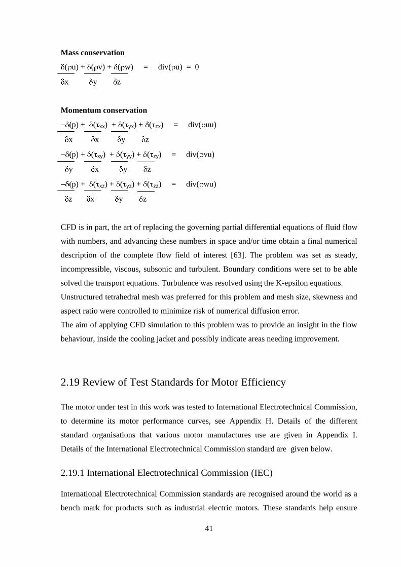
Mass conservation

( u) + ( v) + ( w) = div( u) = 0

x y z

Momentum conservation

p) + ( xx) + ( yx) + ( zx) = div( uu)

x x y z

p) + ( xy) + ( yy) + ( zy) = div( vu)

y x y z

p) + ( xz) + ( yz) + ( zz) = div( wu)

z x y z

CFD is in part, the art of replacing the governing partial differential equations of fluid flow

with numbers, and advancing these numbers in space and/or time obtain a final numerical

description of the complete flow field of interest [63]. The problem was set as steady,

incompressible, viscous, subsonic and turbulent. Boundary conditions were set to be able

solved the transport equations. Turbulence was resolved using the K-epsilon equations.

Unstructured tetrahedral mesh was preferred for this problem and mesh size, skewness and

aspect ratio were controlled to minimize risk of numerical diffusion error.

The aim of applying CFD simulation to this problem was to provide an insight in the flow

behaviour, inside the cooling jacket and possibly indicate areas needing improvement.

2.19 Review of Test Standards for Motor Efficiency

The motor under test in this work was tested to International Electrotechnical Commission,

to determine its motor performance curves, see Appendix H. Details of the different

standard organisations that various motor manufactures use are given in Appendix I.

Details of the International Electrotechnical Commission standard are given below.

2.19.1 International Electrotechnical Commission (IEC)

International Electrotechnical Commission standards are recognised around the world as a

bench mark for products such as industrial electric motors. These standards help ensure

42

that customers will receive consistent product performance and mounting dimensions no

matter where products are applied around the world. The IEC was founded in 1906 as the

result of a resolution passed at the International Electrical Congress held in St. Louis,

Missouri USA in 1904. The purpose of this organisation is to set up consistent standards

for product performance. Examples of relevant standards from this organisation include the

following.

IEC 60034-30 is the latest International Standard, released in November 2008, which

defines the efficiency classes of single speed, three phase, cage induction motors. Within

this standard the Nominal efficiency limits are defined for

Standard Efficiency (IE1)

High Efficiency (IE2)

Premium Efficiency (IE3)

IEC 34-2 is an Electrical Standard, which defines methods for determining losses and

efficiency of Rotating Electrical Machinery from tests.

IEC 72 defines Mechanical Design Properties such as dimensions for rotating electrical

machines.

IEC 61972 is an Electrical Standard, which defines methods for determining losses and

efficiency of three-phase cage induction motors.

IEC specifies five classes of insulation with corresponding temperature rises by resistance.

Class A: 105°C

Class B: 130°C

Class F: 155°C

Class H: 180°C

43

Chapter 3 Experimental/model set-up

3.1 Set-up for current closed cooling system analysis

The system analysed in this work was an ABS closed cooling pump system. This was a

new cooling system introduced by ABS on its M1, M2 and ME3 type pumps in October

2005. A sub-category of the M2 motor type is called a M60/4 motor. This was 6kW four

pole motor that was examined in this work. A schematic of the experimental set-up

designed by ABS Production Wexford is shown in Figure 3.1. A 30% glycol to 70% water

mix coolant was circulated around the motor housing using an impeller attached to the

rotor shaft. Figure 3.2 shows that the returned coolant from the motor housing was

circulated over the heat exchange area at the bottom of the cooling system the opposite side

of which is in contact with the pumped medium. This area was in contact with the pumped

medium which has a maximum allowable temperature of 35 ºC. Tests described below

were implemented to characterise the evolution of the temperature profiles in the pump

environment and in order to examine the effectiveness of the coolant fluid flow through the

pump housing. Unless otherwise indicated, these tests were repeated at least once in order

to ensure confidence in the measured results.

Figure 3-1 Picture of closed cooling experimental set-up with submersible pump

M60/4 submersible pump

Pumped medium return

pipe to water tank

Feeder pipe for 250 m3 water tank

44

Figure 3-2 Close up of heat exchange area

3.1.1 Determination of temperatures generated by the induction motor

For the first experiment the motor was run at full load without cooling jacket. The heat

generation was monitored at four different points around a housing, see Figure 3-3. Point

A, B, C and D indicate the points at which the probes were positioned in the motor

housing. The first probe (point A) was positioned at the top of the motor housing, the

second (point B) was positioned 30mm below this and at 90 degrees clockwise

circumferentially displaced. Points C and D were similarly place beneath this as shown in

Figure 3-4 (b). This gives temperature readings at different heights and different positions

around the housing. One thermocouple was also placed internally located at the upper

bearing, this was used to ensure that the correct temperature rated grease was used on the

bearings. Results were recorded using J-type thermocouples and Anville Instruments

software. The results from this gave exact values of temperature generated by the motor

but most importantly how much heat had to be removed from the system. The pumping

system was also monitored using a FLIR thermal imaging camera. Unlike temperature

probes that give temperature at a particular point, the thermal imaging camera can give an

overall picture as to where most of the heat is generated. The results from this indicated

45

how long the motor can run for without cooling and showed how the heat would propagate

around the housing if no cooling system were in place. This showed the need for a cooling

system.

Figure 3-3 Pictures showing positions of thermocouples on motor housing

(a) positions A and B; (b) positions C and D

Experimental Procedure

Equipment: PC, Anville Instruments data acquisition unit, Roll of J-Type thermocouple,

PTFE tape. M60/4 pump.

1. Prepared thermocouples by stripping the wires at one end and crossing them. Insulated

the thermocouple with PTFE tape. Verified temperature readings across the

temperature range with an infrared non-contact laser Thermometer order code 814-020.

2. Drilled four 5mm holes 5mm deep into the four pre-defined locations around the motor

housing. See Figure 3-3 (a) and (b).

3. Placed thermocouple into each of these holes and secured into place using silicone.

4. Plugged each thermocouple into the data acquisition unit connected to the PC.

5. Started the temperature recording software and then started the motor under full load.

6. Recorded the temperature until it rose above 80 ºC. The test was stopped at this stage to

ensure the protection of the motor winding insulation. This temperature was determined

(a) (b)

46

from a previous experiment where the motor burned out when a temperature of 100 ºC

was reached.

3.1.2Determination of temperatures generated with closed cooling system

This experiment was run at full load according to a similar procedure as described in

section 3.1.1 but with the closed cooling system in place. The temperature rise of the motor

was recorded. The purpose of this experiment was to investigate the effect of the cooling

system to keep the temperature the system stabile and at as low a level as practicable.

Experimental Procedure

1. Prepared thermocouples by stripping the wires at one end and crossing them. Insulated

the thermocouple with PTFE tape.

2. Used the same motor from the previous experiment; disassembled motor housing and

placed one thermocouple on each of the 3 phases.

3. Drilled one 8mm hole at the power cable inlet to allow placement of thermocouples

wires through housing.

4. Re-assembled motor with closed cooling system attached and filled with glycol/water.

5. Plugged each thermocouple into the data acquisition unit connected to the PC.

6. Started the temperature recording software and then started the motor under full load.

7. Recorded the temperature until it the temperature of the system stabilised for a period

of at least 5 minutes.

3.1.3 Determination of temperatures generated with coil cooling system

In the conventional cooling system design, coolant was circulated around the motor

housing. The coolant was forced around using the impeller. The heat was then transferred

out through the heat transfer plate to the medium being pumped through the volute. After

the test described above, it was found that the cooling system did not efficiently extract the

heat or maintain a low temperature within the induction unit. A new design of cooling

system supplied for testing from the casting foundry, LOVINK, Poland, consisted of a

helical mild steel coil integrated into the cast iron motor housing. CAD drawings and

pictures of this design are shown in Figures 3-4 and Appendix G. The diameter of the coil

that could be used was 10 mm. Smaller diameter coils could not be incorporated into the

cast iron with the casting technique as the coil tubing melted in these cases. Given the 15

47

mm housing thickness and potential casting porosity, a 10 mm outer coil diameter was the

largest that could safely be used in order to ensure the housing integrity. This experiment

was run at full load according to a similar procedure as described in section 3.1.1 to

examine the effects of this integrated cooling coil in the motor housing of the M60/4

submersible pump and investigate what effects this would have on the temperature

evolution.

Figure 3-4 SolidWorks model of the coil cooling system.

48

3.1.4 Examination of coolant flow around cooling jacket

For this experiment the motor was run under the same conditions as the previous two

experiments. Unlike the previous two where temperature was examined this experimental

work focused on examining the flow field around the jacket and the flow rate. In order to

determine this, four through slots each 32mm by 92mm were machined into the cooling

jacket and closed off with four corresponding Perspex windows, see figures 3-5 and 3-6.

Two windows were located in the general area above the inlet and the other two were

located at 180º to these in the general area above the outlet of the cooling jacket. These

windows were labelled A, B, C, and D. The glycol in the cooling system was replaced with

3 litres of water seeded with 10% of polypropylene particles (equivalent to 300g) with an

average diameter of 1000 micrometers and a density of 0.96g/cc which is close to that of

water. The motor housing was painted white for clearer visibility of the seeded fluid in the

cooling system. The pump was set to run at the normal operating speed (1490 rpm) and the

flow of the particles was recorded through the windows with a Citius C10 high speed

camera set to record at 330 frames per second. Motor performance curves are shown in

Appendix H. Direction and speed of the fluid flow was determined by analysing the

particle frame to frame movements. The speed of flow was recorded by measuring the

distance of particle displacement between frames and dividing by the time period between

frames (= 1/330 = 3.03 ms). The speed in each of the zones shown in figure 3-6 was

recorded by taking ten separate particle speed measurements and averaging these.

Figure 3-5 top down view of housing locations for windows A, B, C, and D.

49

Figure 3-6 Pictures of Perspex windows A, B, C, and D, showing the

three zones examined for particle speeds.

3.1.5 Determination of flow rate from closed cooling impeller

This experiment determined the flow rate in and out of the cooling jacket. Typically,

stainless steel pipes connect the cooling jacket to the heat exchange area and the closed

cooling impeller. To examine the flow rate within this area, these pipes were replace with

transparent Perspex pipes, the high speed camera was focused on the particles in these

pipes and the images examined as mentioned in section 3.1.3 to calculate the flow rates.

This gives the exact flow rate in the system as the cooling system remains closed and static

head remains the same.

3.1.6 Determination of power consumed by closed cooling system

This experiment was performed to determine power consumed by the cooling system. In

this experiment the pump was run under open shaft (i.e. no pumping load on motor)

conditions and again under open shaft conditions without the cooling impeller and

mechanical seals in place. For both of these tests, the power consumption was monitored

with a Norma D5255 power analyser. This test was designed to determine the power

consumed by the cooling impeller and seals under different speeds and motor types. It was

assumed that the power consumed would the same with impellers in the pump.

50

3.2 Computational Fluid Dynamic (CFD) analysis

3.2.1 Set-up for CFD analysis

CFX (Ver 10.0) was used to model the fluid flow within the examined system. The goal of

this work was to generate a model which would verify the results gained from the

experimental work and then also allow new cooling system designs to be investigated for

potential improved cooling efficiencies. A steady flow set up was sought to provide an

average flow pattern inside the cooling jacket. Faster and more turbulent flows would be

expected to generate better cooling efficiencies. A trial investigation was conducted during

this work to investigate the effect on average coolant speed in the inlet and outlet pipes

with twelve, eight and four blades on the impeller. This showed that the speed of the

coolant flow was greatest for the twelve blade impeller compared to the eight blade

impeller (standard set-up) and was greater for the eight bladed impeller compared to the

four bladed impeller. The steady state housing temperatures measured for the four bladed

and eight bladed systems were 13 °C and 4 °C lower than for the twelve bladed systems

respectively.

A flowchart for the fluid modelling work is shown in Figure 3-8. 3D models of the four

main components of the coolant system were first generated in SolidWorks 2006. These

were exported as IGES files and then imported into ANSYS ICEM CFD where they were

mated, see figure 3-9. In ANSYS CFD, the software allows the user to create two types of

mesh structures, hexahedral meshes and tetrahedral meshes. Tetrahedral (unstructured

mesh) was used due to the complexity of the continuum. Figure 3-10 shows the meshed

upper cooling jacket. The initial modelling was conducted using the default mesh size set

up by ANSYS but this was then refined in order to have more complete mesh coverage of

the volume to be modelled. This was achieved by having a mesh size of 452,387 cells, a

maximum cell aspect ratio of 1:10, and a maximum skewness of cells of 20°. All walls

were set as stationary boundaries except for the impeller which was set as the input

boundary. The input boundary axial velocity, Va, was set to 0 m/s; the radial velocity, VR,

to 0.1 m/s; and the Vθ, was set to the product of the rotational speed (ω) and the radius (r).

A diagram of this boundary is shown in Figure 3-9.

51

Figure 3-7 Flow chart indicting the steps used for model set-up

Figure 3-8 Screen shot of mated structures from ANSYS ICEM CFD

52

Figure 3-9 Meshed continuum of upper cooling jacket

53

Chapter 4 Results

4.1 Introduction

This chapter focuses on the experiments that were carried out on the system to analyse the

strengths and weaknesses of the current closed cooling system. The chapter can be divided

into 3 different sections. The first section presented the current system, the heat build up in

the stator coils and how efficiently the closed cooling system stabilises the temperature

within the system. It is important to remember that for every 10 degrees centigrade rise in

the operating temperature of an induction motor its lifetime is halved. The second section

analyses the flow around the system, to see if the flow was turbulent and uniform around

the motor housing. This was also modelled using CFD software and compared with the

experimental results. This CFD model would allow alternate designs of the cooling system

to be investigated. The CFD model also allowed close examination of the flow around the

heat exchange area. The third and final section examined how the cooling impeller effects

the overall efficiency of the system and how this varies with different motor powers and

poles.

4.1.1 Results of temperatures generated by the induction motor

In this experiment the heat generated when the dry installed motor was operated under full

load without the cooling system attached was investigated. From Figure 4-1 it can be seen

that after 45 minutes without any cooling system, the motor housing was locally at 85 °C

which if left uncooled would eventually lead to the motor burning out and failing. This

experiment was stopped when the motor had reached 108°C. From this result, it is clear

that this submersible pump would not be capable of operating dry installed for long periods

of time without a cooling system. Figure 4-2 shows a thermal image, taken after 1300

seconds, of the pump housing with the colour scale on the right hand side indicating the

level of heat represented by the various colours.

54

Figure 4-1 Housing temperature profiles recorded over a 3500 second period at locations

A, B, C, and D for operation without a cooling system in place

Figure 4-2 Thermal image of the pump housing, taken after 1300 seconds,

without cooling system in place

55

4.1.2. Results of temperatures generated with closed cooling system

This experiment examined the temperature evolution under full load conditions in the

motor with the cooling system in operation. From Figure 4.3 it is clear that this system was

effective as it had stabilised the motor housing at a temperature of 45 °C. This is

approximately 40 °C less compared to the pump set-up without cooling, shown in section

4.1.1. Figure 4-5 displays the thermal image and temperature, taken after 3500 seconds, in

the different areas of the 6kW submersible motor housing. These results showed that the

main areas of heat build up in the system were at either end of the stator where there was a

large area of copper which caused the heat build up. The corresponding temperatures for

the phases, bearing, and pumped water for this system are shown in Appendix B.

10

15

20

25

30

35

40

45

50

015

030

045

060

075

090

010

5012

0013

5015

0016

5018

0019

5021

0022

5024

0025

5027

0028

5030

0031

5033

0034

5036

0037

50

Time (s)

Tem

pera

ture

(deg C

) A

B

C

D

Figure 4-3 Housing temperature profiles recorded over a 4000 second period with a

cooling system in place at locations A, B, C, D

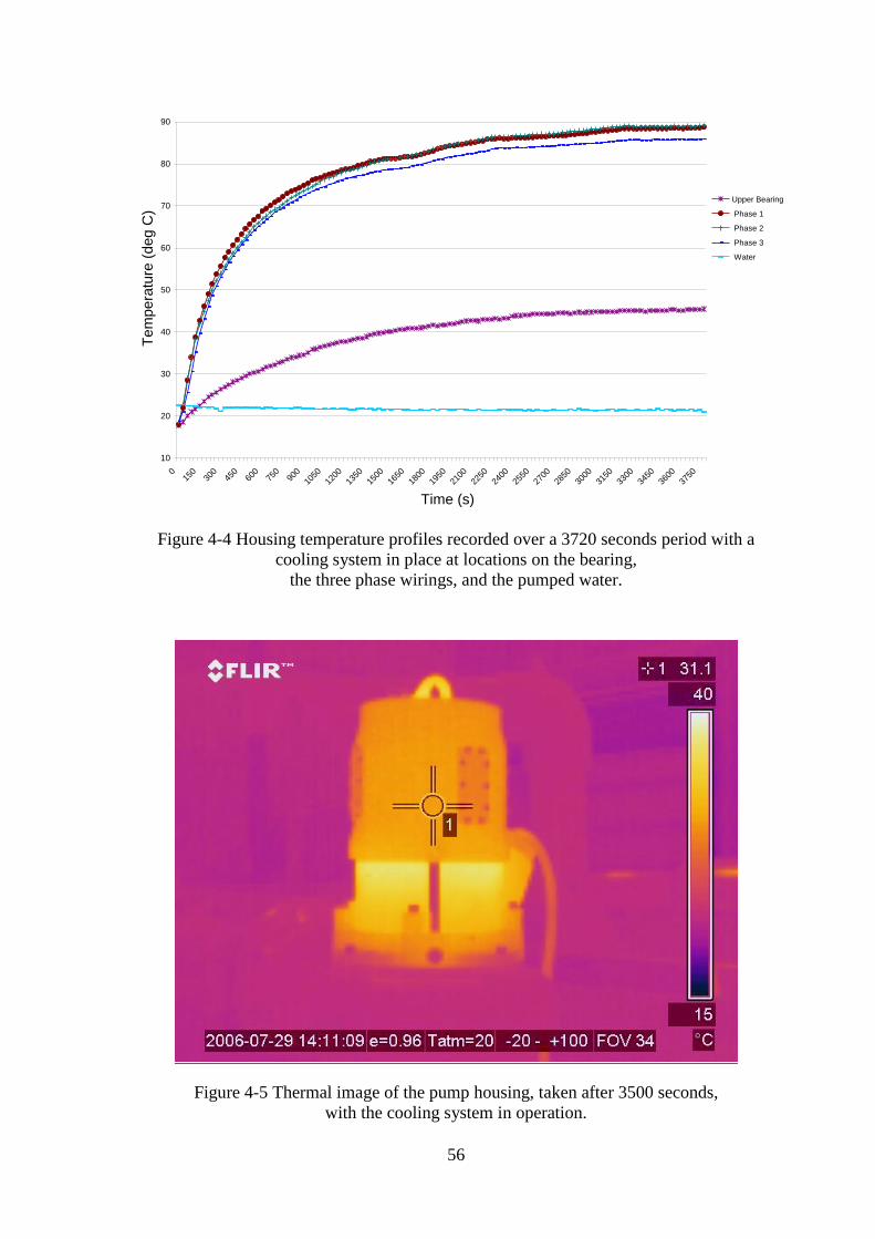
56

10

20

30

40

50

60

70

80

90

015

030

045

060

075

090

0

1050

1200

1350

1500

1650

1800

1950

2100

2250

2400

2550

2700

2850

3000

3150

3300

3450

3600

3750

Time (s)

Te

mp

era

ture

(d

eg

C)

Upper Bearing

Phase 1

Phase 2

Phase 3

Water

Figure 4-4 Housing temperature profiles recorded over a 3720 seconds period with a

cooling system in place at locations on the bearing,

the three phase wirings, and the pumped water.

Figure 4-5 Thermal image of the pump housing, taken after 3500 seconds,

with the cooling system in operation.

57

4.1.3 Results for temperatures generated with coil cooling system

This experiment examined the temperature evolution under full load conditions in the

motor with the coil cooling system in operation. From figure 4-6 it is clear that this system

was as effective as the cooling jacket system as it had stabilised the motor housing at a

temperature of 38 °C. This is approximately 7 °C less compared to the pump set-up with

the closed cooling, shown in section 4.1.2. Figure 4-7 displays the thermal image and

temperature, taken after 3000 seconds, in the different areas of the 6kW submersible motor

housing. The aim was to find any hot spots. These results showed that the main areas of

heat build up in the system were at either end of the stator where there was a large area of

copper which caused the heat build up. The corresponding temperatures for the phases,

bearing, and pumped water for this system are shown in Appendix A.

Following the examination of the coil cooling system using the standard 8 blade impeller, a

second experiment was carried out using a 4 blade impeller. This would give an indication

on what effect a slower flow rate through the system would make on the temperature

gradient. From Figure 4-8 it shows that the lower flow rate through the coils caused less

cooling to take place in the system as a result caused the housing to increase by 7 °C.

10

15

20

25

30

35

40

45

012

024

036

048

060

072

084

096

0

1080

1200

1320

1440

1560

1680

1800

1920

2040

2160

2280

2400

2520

2640

2760

2880

3000

3120

3240

3360

Time (s)

Tem

pera

ture

(deg C

)

A

B

C

Water

Figure 4-6 Temperature rise in cooling system using standard 8 blade impeller.

58

Figure 4-7 Thermal image of the pump housing, taken after 3000 seconds,

with the coil cooling system in operation.

10

15

20

25

30

35

40

45

50

024

048

072

096

0

1200

1440

1680

1920

2160

2400

2640

2880

3120

3360

3600

3840

4080

4320

4560

4800

5040

5280

5520

5760

6000

6240

6480

Time (s)

Te

mp

era

ture

(d

eg

C)

Point A

Point B

Point C

Water

Figure 4-8 Temperature rise in cooling system using a 4 blade impeller

59

4.1.4 Examination of coolant flow around the cooling jacket

After examining the thermal behaviour of the motor the next stage is to understanding the

flow of glycol within the cooling system and to examine whether or not it is functioning to

the optimum level. This is achieved using a high speed camera monitoring four machined

perspex holes machined at either side of the inlet and outlet and the closed cooling system

filled with water saturated with 10% polypropylene with a density of 0.96g/cc. The high

speed camera was used to monitor the flow of these particles within the fluid through each

window and in turn determine the flow at each section within the cooling jacket. The flow

velocity was calculated as the distance travelled by the particle to cross the window (32

mm) divided by the time taken. Appendix D shows the averages and ranges recorded for

flow velocities from analysis ten particles flowing in each window section. The flow field

found form this work is shown in Figure 4-8. The flow path was verified using CFD

analysis.

Figure 4-9 Schematic of the flow field around cooling jacket

60

4.1.5 Results for flow rate from closed cooling impeller

After examining the behaviour of flow around the motor housing the next stage was to

examine the flow into the jacket for both the standard 8 blade impeller and 4 blade

impeller. This was achieved using the high speed camera focused on 50 mm section of

Perspex pipes and capturing a small introduced air bubble passing through the system. This

experiment was carried out on the cooling coils system. The flow velocity was calculated

as the distance travelled by the air bubble to pass through a specified length of pipe

window (50 mm) divided by the time taken. Appendix E and F show the averages and

ranges recorded for flow velocities from the analysis over ten readings. The average fluid

flow speed for the four blade impeller was 176 mm/s and was 217 for the eight blade

impeller.

4.1.6 Results for power consumed by closed cooling system

After examining the behaviour of the cooling system and how the glycol is circulated it is

important to remember that this function comes at a cost, and in this instance its extra

power consumed by the motor. With this extra consumption of power this can affect the

overall efficiency of the electric motor. Table 4-10 shows the experimental pump

configurations and associated power losses. P1 is the input power; P2 is the shaft output

power; PA is the input power with no seals, cooling impeller or collant; PB is the input

power with seals and cooling impeller but with no glycol coolant; PC is same as PB but with

glycol coolant include; Pseal is the power consumed by the seals; Pcoolant is the power

consumed by the coolant; PS+C is the power consumed by seals and impeller; and %Ps+c is

the % power consumed by the seals and impeller.

Motor PA PB PC Pseal Pimpeller Ps+c %Ps+c

Power

P1

(kW)

Power

P2

(kW)

No. of

poles

No

Cartridge

Seal

(W)

With

Cartridge

No

Coolant

(W)

With

Cartridge

With

Coolant

(W )

(W)

(W)

(W)

11.8 10 8 965 1030 1075 65 45 110 0.93%

12.7 11 6 915 1155 1220 240 65 305 2.40%

12.7 11 4 580 870 945 290 75 365 2.87%

22.3 20 2 840 1200 1680 360 480 840 3.77%

28.4 25 2 1050 1700 2086 650 386 1036 3.65%

Table 4-1 Experimental settings and power consumed by open shaft conditions with an

without cooling impeller and seals. (Voltage: 400V; Frequency: 50Hz). Note: the four pole

motor power here was higher than that used in this work; however the trends of efficiency

would be similar

61

0

100

200

300

400

500

600

700

800

900

2 4 6 8

No. Poles

Lo

ss

es

(W

)

Figure 4-10 Graph of the power loss in the motor against the number of motor poles

4.2 Results from Computational Fluid Dynamic (CFD) analysis

CFD results were in agreement with the experimental results. The result shown in Figure 4-

11, that the majority of the flow is in one direction (anticlockwise looking from the top)

around the jacket. This was also proved in section 4.1.4, but what CFD shows us in more

detail is how the liquid behaves before entering the cooling jacket. It shows in detail that

there is a swirling effect in the water as it passes through the feeding pipe. This swirling

effect of the water as it enters the jacket can force the direction of flow in the cooling

jacket in one direction.

Another interesting point from these results is the flow around the heat exchange plate i.e.

flow at the bottom of the screen. It shows that most of the flow occurs around one half of

this plate. From these two findings, optimisation of the flow in the cooling jacket could

lead to a more evenly cooled motor housing with the possibility of hot spots developing

being eliminated. Optimisation around the closed cooling impeller and the heat exchange

plate could certainly result in lower operation temperature of the motor.

62

Figure 4-11 Screen shot of the CFD solution for the closed cooling system

Figure 4-11 Screen shot of the CFD solution for the closed cooling system

The results from the flow chart in Figure 4-12 show in detail how the fluid is behaving in

the system. The screen shot in the middle shows that there is a turbulent flow around the

cooling jacket. Also on the inlet pipe it shows that entrance to inlet pipe going to the jacket,

because of the sudden right angle bend that there is a turbulent flow in this region and in

turn putting unnecessary losses into the cooling system. The return pipe is less critical as

this is a suction line from the jacket. Figure 4-13 displays pressure build up in the system in

Pascal’s. One area for concern from this result is the entrance to the inlet pipe. Because of

the sharp right angle bend this is the area of maximum pressure in the system.

63

Figure 4-12 Flow patterns around the cooling jacket as solved for in CFD

64

Figure 4-13 Screen shot showing pressure in Pa in the closed cooling system

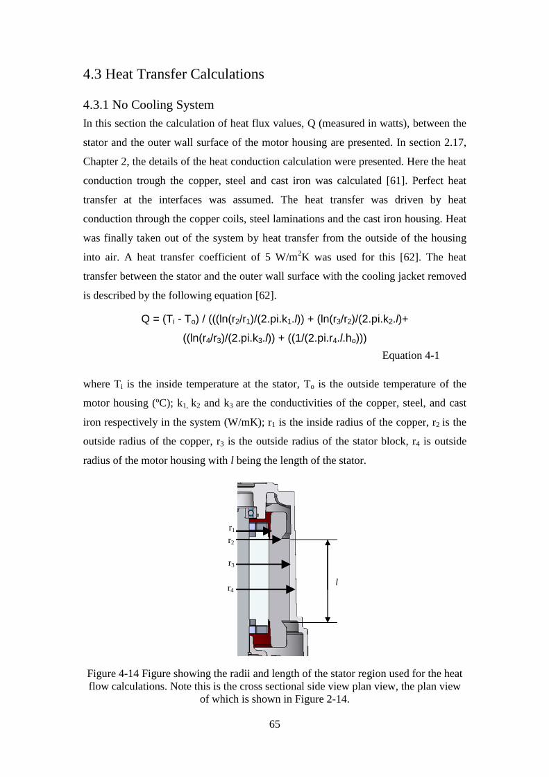
65

4.3 Heat Transfer Calculations

4.3.1 No Cooling System

In this section the calculation of heat flux values, Q (measured in watts), between the

stator and the outer wall surface of the motor housing are presented. In section 2.17,

Chapter 2, the details of the heat conduction calculation were presented. Here the heat

conduction trough the copper, steel and cast iron was calculated [61]. Perfect heat

transfer at the interfaces was assumed. The heat transfer was driven by heat

conduction through the copper coils, steel laminations and the cast iron housing. Heat

was finally taken out of the system by heat transfer from the outside of the housing

into air. A heat transfer coefficient of 5 W/m2K was used for this [62]. The heat

transfer between the stator and the outer wall surface with the cooling jacket removed

is described by the following equation [62].

Q = (Ti - To) / (((ln(r2/r1)/(2.pi.k1.l)) + (ln(r3/r2)/(2.pi.k2.l)+

((ln(r4/r3)/(2.pi.k3.l)) + ((1/(2.pi.r4.l.ho)))

Equation 4-1

where Ti is the inside temperature at the stator, To is the outside temperature of the

motor housing (ºC); k1, k2 and k3 are the conductivities of the copper, steel, and cast

iron respectively in the system (W/mK); r1 is the inside radius of the copper, r2 is the

outside radius of the copper, r3 is the outside radius of the stator block, r4 is outside

radius of the motor housing with l being the length of the stator.

Figure 4-14 Figure showing the radii and length of the stator region used for the heat

flow calculations. Note this is the cross sectional side view plan view, the plan view

of which is shown in Figure 2-14.

r1

r2

r3

r4 l

66

Using the calculation above, the heat transfer Q for the system was calculated. For

this calculation the temperature at the stator coils and the outside of the housing were

taken from the experimental results, see section 4.1.1. From these results, the stator

temperature reached 108°C and an average housing temperature of 85°C was found.

All model parameters are as follows.

Ti = 108 degC r1 = 0.055m

To = 85 degC r2 = 0.07m

k1 = 400 W/mK r3 = 0.08m

k2 = 200 W/mK r4 = 0.09m

k3 = 80 W/mK l = 0.14m

ho = 5 W/m2k

Substituting these values into equation 4-1 gives the following result.

Q = 23/(((0.2412)/(351.68)) + ((0.1335)/(175.84)) + ((0.1178)/(70.336)) + ((1/(0.396)))

Q = 23/((0.00068)+(0.00076)+(0.00167)+(2.528))

Q = 23/2.53

Q = 9.089 W

4.3.2 With Cooling System

In this section the calculation of heat flux values for heat transfer between the stator

and the outer wall surface of the cooling jacket are presented, assuming that there is

cooling fluid in place.

In this model it is assumed as before that conduction of heat occurs through the

copper coils, steel laminations and the cast iron motor housing. Heat transfer between

the motor housing and cooling water; conduction through the cooling liquid; and heat

transfer between the cooling fluid and the cast iron cooling jacket are also taken into

account. Finally conduction through the cooling jacket and heat transfer from the

outside of the housing into air are also incorporated in the model. This model is

represented as follows.

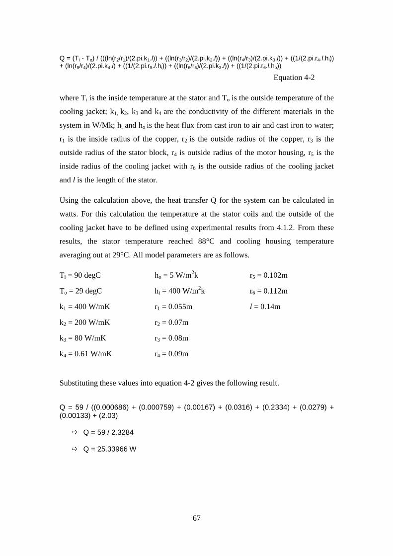
67

Q = (Ti - To) / (((ln(r2/r1)/(2.pi.k1.l)) + ((ln(r3/r2)/(2.pi.k2.l)) + ((ln(r4/r3)/(2.pi.k3.l)) + ((1/(2.pi.r4.l.hi)) + (ln(r5/r4)/(2.pi.k4.l) + ((1/(2.pi.r5.l.hi)) + ((ln(r6/r5)/(2.pi.k3.l)) + ((1/(2.pi.r6.l.ho))

Equation 4-2

where Ti is the inside temperature at the stator and To is the outside temperature of the

cooling jacket; k1, k2, k3 and k4 are the conductivity of the different materials in the

system in W/Mk; hi and ho is the heat flux from cast iron to air and cast iron to water;

r1 is the inside radius of the copper, r2 is the outside radius of the copper, r3 is the

outside radius of the stator block, r4 is outside radius of the motor housing, r5 is the

inside radius of the cooling jacket with r6 is the outside radius of the cooling jacket

and l is the length of the stator.

Using the calculation above, the heat transfer Q for the system can be calculated in

watts. For this calculation the temperature at the stator coils and the outside of the

cooling jacket have to be defined using experimental results from 4.1.2. From these

results, the stator temperature reached 88°C and cooling housing temperature

averaging out at 29°C. All model parameters are as follows.

Ti = 90 degC ho = 5 W/m2k r5 = 0.102m

To = 29 degC hi = 400 W/m2k r6 = 0.112m

k1 = 400 W/mK r1 = 0.055m l = 0.14m

k2 = 200 W/mK r2 = 0.07m

k3 = 80 W/mK r3 = 0.08m

k4 = 0.61 W/mK r4 = 0.09m

Substituting these values into equation 4-2 gives the following result.

Q = 59 / ((0.000686) + (0.000759) + (0.00167) + (0.0316) + (0.2334) + (0.0279) + (0.00133) + (2.03) Q = 59 / 2.3284

Q = 25.33966 W

68

4.3.3 With Coil Cooling System

This section calculates the Q value for heat transfer between the stator and the outer

wall surface of the motor housing/ cooling jacket. It solves for Q given that the system

is conducting heat through the copper coils, steel laminations and the cast iron motor

housing, convection between the motor housing and the coil cooling system,

conduction through the cooling liquid, convection between the coil cooling system

and the motor housing, conduction through the motor housing and finally convecting

the heat away from the outside of the housing into air. This model is represented as

follows.

Q = (Ti - To) / (((ln(r2/r1)/(2.pi.k1.l)) + ((ln(r3/r2)/(2.pi.k2.l)) + ((ln(r6/r3)/(2.pi.k3.l)) + ((1/(2.pi.r4.l.hi)) + (ln(r5/r4)/(2.pi.k4.l) + ((1/(2.pi.r5.l.hi)) + ((ln(r6/r3)/(2.pi.k3.l)) + ((1/(2.pi.r6.l.ho))

Equation 4-3

Where Ti is the inside temperature at the stator and To is the outside temperature of

the cooling jacket. k1, k2, k3 and k4 are the conductivity of the different materials in the

system in W/mK. hi and ho is the heat flux from cast iron to air and cast iron to water.

The dimension, r1 is the inside radius of the copper, r2 is the outside radius of the

copper, r3 is the outside radius of the stator block, r4 is outside radius of the motor

housing, r5 is the inside of the cooling coils, r6 is the outside radius of the cooling

coils and l is the length of the stator.

Using the calculation above, the heat transfer Q for the system can be calculated in

watts. For this calculation the temperature at the stator coils and the outside of the

cooling jacket have to be defined using experimental results from 4.1.3. From these

results, the stator temperature reached 105°C and cooling housing temperature

averaging out at 37°C. All model parameters are as follows.

Ti = 105 degC ho = 5 W/m2k r5 = 0.095m

To = 37 degC hi = 400 W/m2k r6 = 0.1m

k1 = 400 W/mK r1 = 0.055m l = 0.14m

k2 = 200 W/mK r2 = 0.07m

k3 = 80 W/mK r3 = 0.08m

k4 = 0.6 W/mK r4 = 0.085m

69

Substituting these values into equation 4-3 gives the following result.

Q = 68 / (0.000686) + (0.00076) + (0.00317) + (0.00335) + (0.2108) + (0.002993) + (0.00317) + (2.27) Q = 68 / 2.5

Q = 27.2 W

4.3.4 Coil Cooling System with 4 Blade Impeller

This section calculates the Q value for the same cooling coil system as in 3.3.3 but

standard closed cooling 8 blade impeller was replaced with a 4 blade impeller in order

to slow down the flow rate around the jacket. The equation remains the same as the

physical components of the system remain the same.

Using the same calculation from 3.3.3 and the experimental results from 4.1.3 where

the stator temperature reached 114°C and cooling housing temperature averaging out

at 46°C. All model parameters are as follows.

Ti = 114 degC ho = 5 W/m2k r5 = 0.095m

To = 46 degC hi = 400 W/m2k r6 = 0.1m

k1 = 400 W/mK r1 = 0.055m l = 0.14m

k2 = 200 W/mK r2 = 0.07m

k3 = 80 W/mK r3 = 0.08m

k4 = 0.6 W/mK r4 = 0.085m

The same equation as Equation 4-3 is used here with the above parameters used

instead.

Q = 68 / (0.000686) + (0.00076) + (0.00317) + (0.00335) + (0.2108) + (0.002993) + (0.00317) + (2.27) Q = 68 / 2.5

Q = 27.2 W

These two results for the coil cooling system show that the heat transfer from the

stator to the outer wall remained the same and that the key area from a cooling point

of view is the heat transfer plate which separates the pumped medium from the

cooling liquid.

70

Chapter 5 Conclusion and Recommendations

5.1 Conclusions

In the present study, the analysis of the current closed cooling system showed that it is

capable of maintaining the system steady state operating temperature within the IEC

temperatures ranges as specified in section 2.21.1. It was found that all the closed

loop cooling systems in this work met the Class H insulation. However, examination

into the cooling systems showed that variations in efficiencies between different

systems. The results from section 4.1.1 and 4.2.1 show that the use of the cooling

jacket markedly reduced the external motor housing temperature, see Figure 4-1 and

Figure 4-3. On examination of fluid flow around the outer jacket, see section 4.1.4, it

was found that the flow occurred in one direction and that the closed cooling

effectively only occurred from three quarters of the motor housing. Results from

section 4.1.3, showed that elimination of this dormant area and creating a fluid flow

around the motor housing reduced the operational temperature of the motor by 7 °C ,

see Figure 4-3 and Figure 4-6.

The CFD results in Figure 4-11, show that the area around the heat exchange plate has

potential for optimization as the fluid flow is not uniformly distributed over the heat

exchange plate (housing body) and hence heat transfer is not maximised. The

introduction of a spiral or a baffle like shape into the casting could create a directional

flow over the entire area and prolong the cooling fluid contact with the heat exchange

plate. This could have an additional beneficial effect in the overall performance of the

cooling system by reducing the motor operational temperature.

Analysis of the power measurements taken in section 4.1.6, showed that for a 4 pole

motor the power consumed by the cooling impeller was 75 watts, which represents

1.25% of power consumed from a 6kW motor. Future work could investigate different

impeller designs in order to improve the flow around the heat exchange plate as well

as increasing impeller efficiency. From Table 4.1, it can be seen that the same

impeller which is used on a two pole and four pole motor consumes over six times

more power on the four pole motor even though the power rating is only twice that of

the two pole motor. This indicates that optimised impeller designs could be produced

71

for different speed motors. Improvement in this area can lead to improved cooling

characteristics and reduction in the power consumed by the system.

This work has shown the potential for optimizing the cooling system. A more efficient

cooling system would yield a cooler motor, which in turn would give a better motor

efficiency and longer motor life also.

5.2 Recommendations for Future Work

The results in the present study are significant; however the future work in relation to

the present study can be listed as follows:

Baffles

The heat transfer plate situated between the pumped medium and cooling fluid

could be looked at further by optimising the design to include spiral ribs or baffles

on the cooling fluid side. This could optimise flow around this plate and also

increase the surface area to transfer heat away.

Inlet/Outlet pipes

Sharp right angle bends from the inlet pipe could be removed to improve coolant

speed and promote flow direction. Sharp bends add losses to the system and

reducing the flow rate into the cooling jacket. Results from section 4.1.3 show that

as the flow rate in the system reduces the temperature of the stator housing

increases.

Motor Speed

Further investigation of the effect of motor speeds on the efficiencies and capacity

of the cooling system could be investigated.

Deflector plate

The closed cooling deflector plate could be optimised to direct the flow into the

closed cooling impeller and to direct flow around the heat exchange plate. in

order to reduce power consumed by the motor, reduce the running temperature

motor and increase the overall running efficiency of the motor.

72

References

[1] R. Lomas, The man who invented the twentieth century - forgotten genius,

Headline Book Publishing, 1999, ISBN: 978-0747275886.

[2] www.flowserve.com, accessed 9/10/2005

[3] J. Mokander, How Efficiency of A-C induction motor is determined, Publisher in

Scientific Impeller, 2002.

[4] P.B.Greenwood, Energy efficiency report, Brook Crompton Parkinson Motors,

1996.

[5] http://www.lmphotonics.com/energy.htm, accessed 13/2/2006

[6] http://www.sapiensman.com/topics/topics_7.htm, accessed 10/10/2005.

[7] http://www.ndt-

ed.org/EducationResources/HighSchool/Magnetism/electricmotor.htm, accessed

2/11/2005

[8] http://electronics.howstuffworks.com/motor1.htm, accessed 21/1/2007.

[9] A.O. Smith Electical Compontents Bulletin #3100, The AC’s and DC’s of Electric

Motors, 2002.

[10] http://hyperphysics.phy-astr.gsu.edu/hbase/magnetic/mothow.html, accessed

11/10/2005

[11] http://www.phys.unsw.edu.au, accessed 10/10/2005

[12] K, Rajashekara, Sensorless Control of AC Motors, Published by IEEE Press,

October 1996.

[13] http://www.play-hookey.com/ac_theory/ accessed 12/2/2006

[14] S. Gibilisco, Teach yourself electricity and electronics, McGraw-Hill, 2006,

ISBN: 978-0071459334.

[15] http://www.oddparts.com/acsi/motortut.htm, accessed 10/10/2005

[16] http://www.tpub.com/neets/book5/18a.htm, accessed 22/8/2006

[17] http://www.reliance.com/mtr/mtrthrmn.htm, accessed 1/9/2006

[18] T.C. Martin and N. Tesla, The Tesla Rotating Magnetic Field, Kessinger

Publishing, 2005.

[19] http://www.tpub.com/neets/book5/18a.htm, accessed 6/04/2006

73

[20] I. Gottlieb, Practical Electric Motor Handbook, Newnes, 1997, ISBN: 978-

0750636384.

[21] F. Alonge and F. D’Ippolito, Design and sensitivity analysis of a reduced-order

rotor flux optimal observer for induction motor control, Control Engineering Practice,

Vol. 15 Issue 12, Dec 2007

[22] C.-S. Chiu, K.-Y. Lian, C.-Y. Hung, and P. Liu, , International Journal of

Control, Feb2008, Vol. 81 Issue 2

[23] http://www.kilowattclassroom.com/Archive/SyncMotors.pdf, accessed 21/5/2006

[24] P.D. Malliband, Design of a double-jacketed, closed type calorimeter for direct

measurement of motor losses, IEE Conference Publication, 1998.

[25] V. Viktor, Induction motor field-oriented controller, respecting iron losses,

International Symposium on Industrial Electronics, IEEE, 1995.

[26] I. Gottlieb, Electric Motors and Control Techniques, McGraw-Hill Professional,

1994.

[27] I.A. Metwally and A. Gastli, Correlation between eddy currents and corrosion in

electric submersible pump systems, International Journal of Thermal Sciences,

Elsevier, Volume 47, Issue 6, 2008, pp. 800-810.

[28] H.W. Beaty and J.L. Kirtley, Electric Motor Handbook, McGraw Hill, 1998,

ISBN: 978-0070359710.

[29] A.J. Pansini, Basics of Electric Motors, PennWell Books, 1996

[30] http://en.wikipedia.org/wiki/Electric_motor, accessed 9/10/2005.

[30] R.R. Lawrence, Principles of Alternating Current Machinery, McGraw-Hill,

1920.

[31] M. Gussow, Schaum's Outline of Theory and Problems of Basic Electricity,

McGraw-Hill, 2004.

[32] http://science.jrank.org/pages/2314/Electric-Motor-Principles-three-phase-motor-

operation.html, accessed 10/10/2006

[34] S. Whatley and A. Berry, Overall energy efficiency practices, World Pumps,

Volume 2008, Issue 500, May 2008, pp. 56-58.

[35] R. Montenegro and N. Hökby, Pump Life Cycle Costs, a guide to LCC analysis

for pumping systems, World Pumps, Volume 2004, Issue 451, April 2004, pp. 35-36.

[36] http://www.oddparts.com/acsi/defines/poles.htm, accessed 10/03/2006.

74

[37] S.L. Herman, Industrial Motor Control, Thomson Delmar Learning – Publisher,

1998, ISBN: 978-0827386402.

[38] M.A. El-Sharkawi, Electric Energy: An Introduction, CRC Press, 2004, ISBN

0849330785.

[39] H.W. Beaty and J.L. Kirtley, Electric Motor Handbook, McGraw-Hill

Handbooks, 1998, ISBN: 978-0070359710.

[40] http://hyperphysics.phy-astr.gsu.edu/hbase/electric/powfac.html, accessed

17/11/2005

[41] F. Alonge and F. D’Ippolito, Design and sensitivity analysis of a reduced-order

rotor flux optimal observer for induction motor control, Control Engineering

Practice, Volume 15, Issue 12, 2007, pp. 1508-1519.

[42] P. Laplante, Comprehensive Dictionary of Electrical Engineering, CRC Press,

1998, ISBN: 978-0849331282.

[43] C.P. Steinmetz, Theory and Calculations of Electrical Apparatus, McGraw-Hill,

1917.

[45] H.B. Metwally, New method for speed control of single phase induction motor

with improved motor performance, Energy Conversion and Management,

Volume 42, Issue 8, May 2001, pp. 941-950

[46] A.R. Muñoz, Using an autoregressive model in the detection of abnormal

characteristics of squirrel cage induction motors, Electric Power Systems Research,

Volume 55, Issue 2, 2000, pp. 73-77.

[47] I. J. Cameron, W.T. Thomson and A.B. Dow, Vibration and current monitoring

for detecting airgap eccentricity in large induction motors. IEE Proc. Part B 133 3

(1986), pp. 155–163. View Record in Scopus | Cited By in Scopus (78)

[48] R.R. Schoen and T.G. Habetler, Effects of time-varying loads on rotor fault

detection in induction machines. IEEE Trans. Ind. Applic. 31 4 (1995), pp. 900–906.

Full Text via CrossRef | View Record in Scopus | Cited By in Scopus (44)

[49] J.F. Watson, S. Elder, Transient analysis of the line current as a fault detection

technique for three phase induction motors, in: Proceedings of International

Conference on Electrical Machines, Manchester, UK, vol. 3, 15–17 September, 1992,

pp. 1241–1245.

[50] H.A. Toliyat and T.A. Lipo, Transient analysis of cage induction machines under

stator, rotor bar and end ring faults. IEEE Trans. Energy Conv. 10 2 (1995), pp. 241–

247.

[51] http://www.lmphotonics.com/m_control.htm accessed 10/3/2006

75

[52] L. L. Grigsby, The Electric Power Engineering Handbook, CRC Press, 2000,

ISBN: 978-0849385780.

[53] http://www.lmphotonics.com/m_control.htm accessed 10/10/2005

[54] http://www.powertecmotors.com/ferrite.html accessed 3/11/2005

[55] A.L. Sheldrake, Handbook of Electrical Engineering: For Practitioners in the Oil,

Gas and Petrochemical Industry, Wiley, 2003, ISBN: 978-0-471-49631-1.

[56] R.H. Knight, G.R. Webster, T.A. Flyen,.A novel induction motor suitable for use

in a potentially explosive atmosphere, Electrical Machines and Drives, 1993. Sixth

International Conference.

[57] R. T. Hudson, J. Rockwell, A. Parker, Application of Temperature Ratings for

Industrial Electric Induction Motors, CO; This paper appears in: 53rd Annual

Petroleum and Chemical Industry Conference, 2006. Industry Applications Society.

[58] http://en.wikipedia.org/wiki/Power_factor_correction; accessed 08/08/2007

[59] http://www.lmphotonics.com/m_control.htm; accessed 08/08/2007

[60] http://www.energy-in-motion.com/PFC.html; accessed 08/08/2007

[61] F.P. Incropera, D.P. DeWitt, T.L. Bergman, A.S. Lavine, Fundamentals of Heat

and Mass Transfer, Wiley; 6 Ed., 2006, ISBN-10: 0471457280.

[62] W.M. Rohsenow, J.P. Hartnett, Y.I. Cho, Handbook of Heat Transfer, McGraw-

Hill Professional; 3 Ed., 1998, ISBN-10: 0070535558.

[63] J.F. Wendt, Computational Fluid Dynamics An Introduction, Springer-Verlag,

1991, ISBN-10: 3540850554

76

Appendix – A

Performance of the closed cooling impeller

Head (m) Flow (l/s)

Average Flow speed

(m/s)

0 0.09 0.114

0.2 0.075 0.095

0.4 0.06 0.076

0.6 0.045 0.057

0.8 0.023 0.029

1 0 0

Appendix - B

Temperautres of the the bearing, water and phases

0

10

20

30

40

50

60

70

80

90

100

012

024

036

048

060

072

084

096

0

1080

1200

1320

1440

1560

1680

1800

1920

2040

2160

2280

2400

2520

2640

2760

2880

3000

3120

3240

3360

3480

3600

3720

Time

Te

mp

Bearing

Phase 1

Phase 2

Phase 3

Water

.

77

Appendix - C

Theraml image temperature profiles for coil cooling system

Temperature at outlet to motor is 28 C

Temperature at inlet to motor is 27 C

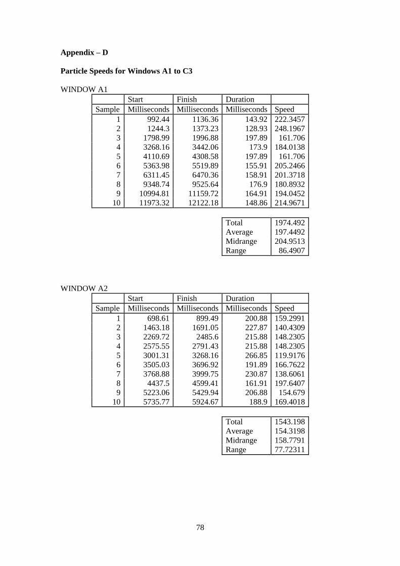
78

Appendix – D

Particle Speeds for Windows A1 to C3

WINDOW A1

Start Finish Duration

Sample Milliseconds Milliseconds Milliseconds Speed

1 992.44 1136.36 143.92 222.3457

2 1244.3 1373.23 128.93 248.1967

3 1798.99 1996.88 197.89 161.706

4 3268.16 3442.06 173.9 184.0138

5 4110.69 4308.58 197.89 161.706

6 5363.98 5519.89 155.91 205.2466

7 6311.45 6470.36 158.91 201.3718

8 9348.74 9525.64 176.9 180.8932

9 10994.81 11159.72 164.91 194.0452

10 11973.32 12122.18 148.86 214.9671

Total 1974.492

Average 197.4492

Midrange 204.9513

Range 86.4907

WINDOW A2

Start Finish Duration

Sample Milliseconds Milliseconds Milliseconds Speed

1 698.61 899.49 200.88 159.2991

2 1463.18 1691.05 227.87 140.4309

3 2269.72 2485.6 215.88 148.2305

4 2575.55 2791.43 215.88 148.2305

5 3001.31 3268.16 266.85 119.9176

6 3505.03 3696.92 191.89 166.7622

7 3768.88 3999.75 230.87 138.6061

8 4437.5 4599.41 161.91 197.6407

9 5223.06 5429.94 206.88 154.679

10 5735.77 5924.67 188.9 169.4018

Total 1543.198

Average 154.3198

Midrange 158.7791

Range 77.72311

79

WINDOW A3

Start Finish Duration

Sample Milliseconds Milliseconds Milliseconds Speed

1 1529.14 1819.98 290.84 110.0261

2 2254.73 2470.61 215.88 148.2305

3 2398.65 2695.48 296.83 107.8058

4 2860.39 3223.19 362.8 88.20287

5 3244.17 3564.99 320.82 99.7444

6 3636.95 3837.84 200.89 159.2912

7 3936.78 4293.58 356.8 89.6861

8 4218.63 4569.43 350.8 91.22007

9 4863.26 5247.05 383.79 83.37893

10 5181.08 5504.9 323.82 98.82033

Total 1076.406

Average 107.6406

Midrange 121.335

Range 75.91222

WINDOW B1

Start Finish Duration

Sample Milliseconds Milliseconds Milliseconds Speed

1 140.92 326.82 185.9 172.1356

2 575.68 779.56 203.88 156.9551

3 1229.31 1412.21 182.9 174.959

4 1891.94 1984.88 92.94 344.3082

5 2194.76 2395.65 200.89 159.2912

6 6599.29 6773.19 173.9 184.0138

7 6785.18 6974.07 188.89 169.4108

8 6938.1 7141.98 203.88 156.9551

9 7204.94 7381.85 176.91 180.8829

10 7468.84 7600.72 131.88 242.6448

Total 1941.556

Average 194.1556

Midrange 250.6316

Range 85.68976

80

WINDOW B2

Start Finish Duration

Sample Milliseconds Milliseconds Milliseconds Speed

1 860.52 1142.36 281.84 113.5396

2 2035.85 2284.71 248.86 128.5864

3 3729.9 3942.78 212.88 150.3194

4 4650.38 5001.59 351.21 91.11358

5 5765.75 5969.64 203.89 156.9474

6 6200 6365.42 165.42 193.447

7 8242.36 8392.28 149.92 213.4472

8 8431.25 8584.17 152.92 209.2597

9 8728.09 8869.01 140.92 227.0792

10 11024.8 11141.73 116.93 273.668

Total 1757.407

Average 175.7407

Midrange 182.3908

Range 182.5544

WINDOW B3

Start Finish Duration

Sample Milliseconds Milliseconds Milliseconds Speed

1 2107.81 2494.6 386.79 82.73223

2 3022.3 3343.12 320.82 99.7444

3 5711.79 5960.65 248.86 128.5864

4 6845.15 7273.91 428.76 74.63383

5 7627.71 7846.58 218.87 146.2055

6 9240.8 9498.65 257.85 124.1032

7 9822.47 10242.24 419.77 76.23222

8 10338.18 10662 323.82 98.82033

9 13219.56 13450.43 230.87 138.6061

10 13684.3 13945.15 260.85 122.6759

Total 1092.34

Average 109.234

Midrange 106.62

Range 69.97329

81

WINDOW

C1 Start Finish Duration

Sample Milliseconds Milliseconds Milliseconds Speed

1 491.72 680.62 188.9 169.4018

2 1166.34 1352.24 185.9 172.1356

3 1247.3 1445.19 197.89 161.706

4 1789.99 2023.86 233.87 136.8282

5 2266.72 2449.62 182.9 174.959

6 2416.64 2590.54 173.9 184.0138

7 2620.53 2791.43 170.9 187.244

8 2926.35 3103.25 176.9 180.8932

9 3993.75 4149.66 155.91 205.2466

10 4710.35 4947.22 236.87 135.0952

Total 1707.523

Average 170.7523

Midrange 170.1709

Range 70.15142

WINDOW C2

Start Finish Duration

Sample Milliseconds Milliseconds Milliseconds Speed

1 167.91 344.81 176.9 180.8932

2 1163.35 1337.25 173.9 184.0138

3 2041.85 2209.76 167.91 190.5783

4 2494.6 2773.44 278.84 114.7612

5 4380.53 4575.42 194.89 164.1952

6 4710.35 4917.23 206.88 154.679

7 5097.13 5345.99 248.86 128.5864

8 6044.6 6275.47 230.87 138.6061

9 7480.79 7669.68 188.89 169.4108

10 7801.61 8029.48 227.87 140.4309

Total 1566.155

Average 156.6155

Midrange 159.5823

Range 61.99193

82

WINDOW C3

Start Finish Duration

Sample Milliseconds Milliseconds Milliseconds Speed

1 422.76 638.64 215.88 148.2305

2 1873.95 2170.78 296.83 107.8058

3 2569.55 2836.4 266.85 119.9176

4 2809.42 3067.27 257.85 124.1032

5 3169.22 3514.02 344.8 92.80742

6 3585.98 3933.79 347.81 92.00426

7 4071.71 4374.54 302.83 105.6698

8 4434.5 4716.35 281.85 113.5356

9 5133.11 5507.9 374.79 85.38115

10 6254.48 6546.37 291.89 109.6303

Total 1099.086

Average 109.9086

Midrange 116.8058

Range 62.84935

83

Appendix – E

Fluid Velocity Through Inlet Pipe Using 8 Blade Impeller

Start Finish Duration

Sample Milliseconds Milliseconds Milliseconds Speed

1 612.66 844.28 231.62 215.8708

2 260.73 485.32 224.59 222.6279

3 235.74 466.68 230.94 216.5065

4 1058.35 1291.43 233.08 214.5186

5 604.46 831.85 227.39 219.8865

6 160.92 390.89 229.97 217.4197

7 311.54 542.32 230.78 216.6566

8 843.47 1071.46 227.99 219.3079

9 499.18 729.27 230.09 217.3063

10 379.23 608.08 228.85 218.4837

Total 2178.584

Average 217.8584

Midrange 218.5733

Range 8.10928

Appendix – F

Fluid Velocity Through Inlet Pipe Using 4 Blade Impeller

Start Finish Duration

Sample Milliseconds Milliseconds Milliseconds Speed

1 163.53 444.23 280.7 178.1261

2 401.85 685.88 284.03 176.0377

3 494.79 776.72 281.93 177.349

4 970.31 1254.26 283.95 176.0873

5 411.52 691.37 279.85 178.6671

6 107.61 390.68 283.07 176.6348

7 240.47 525.83 285.36 175.2173

8 434.61 718.53 283.92 176.1059

9 254.84 535.31 280.47 178.2722

10 576.13 858.35 282.22 177.1667

Total 1769.664

Average 176.9664

Midrange 176.9422

Range 3.449874

84

Appendix – G

Schematics of Coil Cooling System

85

Appendix – G

Schematics of Coil Cooling System

86

Appendix – H

Motor Performance curve

Appendix – I

87

Appendix – I Motor Test Standards

British Standard BS EN 60034-1:1998

Rotating electrical machines – Part 1: Rating and performance

Section 2. Definitions

Rated Value:

A value assigned usually by the manufacturer for a specified operating condition of a

machine

Rating:

The set of rated values and operating conditions

Rated Output:

The value of the output included in the rating

Load:

All the values of the electrical and mechanical quantities that signify the demand

made on a rotating machine by an electrical circuit or a mechanism at a given instant

No-Load:

The state of a machine rotating with zero output power

Full Load:

The load which causes a machine to operate at its rating

Full Load Value:

A quantity value for a machine operating at full load

Rest and de-energise:

The complete absence of all movement and of all electrical supply or mechanical

drive

88

Duty:

The statement of the load to which the machine is subjected

Duty Type:

One or more loads remaining constant for the duration specified within the

permissible operating range

Cyclic duration factor:

Ratio between period of loading and the duration of the duty cycle

Locked Rotor Torque:

The smallest measured torque the motor develops at its shaft with the rotor locked

Locked Rotor Current:

The greatest steady-state r.m.s. current taken from the line with the motor held at rest

Pull up torque:

The smallest value of torque which the motor develops between zero speed and the

speed which corresponds to the breakdown torque when the motor is supplied at the

rated voltage and frequency

Breakdown torque:

The maximum value of the steady state torque which the motor develops without an

abrupt drop in speed

Pull out torque:

The maximum torque which the motor develops at operating temperature and at

synchronous speed

Cooling:

A procedure by means of which heat resulting from losses occuring in a machine is

given up to a primary coolant

Primary coolant:

A medium being at a lower temperature than a part of a machine and in contact with

it, removes heat from the part

89

Secondary coolant:

Removes the heat given up by the primary coolant by means of a heat exchanger or

through the external surface of the machine

Direct cooled winding:

A winding mainly cooled by the coolant flowing in direct contact with the cooled part

through hollow conductors, form an integral part of the winding inside the main

insulator

Indirect cooled winding:

Any winding other than the direct cooled winding

Supplementary insulator:

An independent insulation applied in addition to the main insulation in order to insure

protection against electric shock in the event of failure of the main insulation

Moment of inertia:

The sum of the products of the mass elements of a body and the squares of their

distances from a given axis

Thermal equilibrium:

The state reached when the temperature rises of the several parts of the machine do

not vary by more than a gradient of 2 K per hour.

Thermal equivalent time constant:

The time constant which determines approximately the temperature course in a

winding after a step wise current change

Encapsulated winding:

A winding, which is completely enclosed or sealed by moulded insulation.

Section 4. Rating

Assignment of Rating:

The manufacturer shall assign the rating, the designation of the class of rating shall be

written after the rated output.

90

International Standard IEC 34-2

Rotating electrical machines – Methods for determining losses and efficiency of

rotating electrical machinery from tests (excluding machines for traction

vehicles)

Determination of Efficiency:

Total loss measurement:

Electrical back to back tests:

When identical machines are run at essentially the same rated conditions, the losses

supplied from the electrical system are assumed to be equally distributed and the

efficiency is calculated from half the total losses and the electrical input. This test is

carried out as near as possible at the temperature attained in operation. This is so no

winding temperature correction shall be made.

Direct measurement of efficiency:

Braking Test:

When the machine is run at rated conditions of speed, voltage and current, the

efficiency is then taken as the ratio of output to input. The test shall be made as nearly

as possible at the temperature attained in operation at the end of the time specified in

the rating. No winding temperature correction shall be made.

Calibrated Machine Test:

When the machine is run at rated conditions of speed, voltage and current, the

efficiency is taken as the ratio of output to input

Mechanical back to back test:

When identical machines are run at essentially the same rated conditions, the losses

are assumed to be equally distributed and the efficiency is calculated from half the

total losses and electrical input.

Zero Power Factor Test

When the machine is run at rated conditions of speed, voltage and current, the total

losses are equivalent to the absorbed power during the test, corrected for the

difference between actual and the full-load exciting current losses.

91

Retardation Method:

This method can be used for determining the separate losses of rotating electrical

machines.

Sum of the friction loss and windage loss in machines of all types.

Sum of losses in active iron and additional open-circuit losses in D.C. and

synchronous machines.

Sum of I²R losses in an operating winding and additional load loss in synchronous

machines.

Losses:

Losses can be measured using all of the test methods mentioned previously.

Load Losses:

These consist of I²R losses in primary windings. The I²R losses in the primary

winding are normally measured during the short-circuit test. The losses are calculated

from the rated current and the resistance of the windings corrected to the reference

temperature.

Additional Load Losses:

Unless otherwise specified, it is assumed that the additional load losses vary as the

square of the armature current.

92

IEEE 112 Standard Test Procedure for Polyphase Induction Motors and

Generators

This standard provides the basic test procedure for evaluating the performance of a

polyphase induction motor or generator of any size

Tests with Load:

Tests with load are made for the determination of efficiency, power factor, speed,

current and temperature rise. Some of the miscellaneous tests outlined in clause 9 are

also made with load. For all tests with load, the machine shall be properly aligned and

securely fastened.

Tests with Rotor Locked:

Testing of induction motors under locked-rotor conditions involves high mechanical

stresses and high rates of heating. Locked rotor gives you the starting voltage and

current of a motor. The direction of rotation should be established before the test and

readings should be taken as quickly as possible to avoid motor burn out.

Mechanical Power Test:

Power is calculated using the following formula

Power (in W) = T = (T*n)/k

T is torque

n is the rotational speed in r/min

k is 9.549, if T is in N * m

k is 7.043, if T is in 1bf * ft

A dynamometer is used to determine torque and speed of the test machine shaft.

Bearing Loss Stabilisation:

Some motors may experience a change in friction loss until the bearings reach a

stabilized operating condition. Stabilisation will not occur until there is no excess

grease present in the path of the moving parts.

93

Types of Losses:

Stator Loss:

Stator I²R loss in watts is equal to 1.5 I²R for three phase motors.

I is the measured or calculated rms current per line terminal at the specified load

R is the dc resistance between any two line terminals corrected to the specified

temperature

Rotor Loss:

Rotor I²R loss should be determined from the per unit slip, whenever the slip is

accurately determinable using the following equation.

Motor rotor I²R loss = (measured stator input power – stator I²R loss – core loss) * s

Core, Friction and Windage Loss:

These values are calculated by the no load test as outlined in section 5.3

Determination of Efficiency:

Efficiency is the ratio of output power to total input power. Output power is equal to

input power minus the losses. If two of the three variables are known, the efficiency

can be determined by one of the following equations

Efficiency = output power / input power

Efficiency = (input power – losses) / input power

Efficiency = output power / (output power + losses)

Test Method for Efficiency:

Test Method B – Input – output with loss segregation:

This method is made up of several tests. The apparent total loss is segregated into its

various components with stray –load loss defined as the difference between the

apparent total loss and the sum of the conventional losses, i.e. the stator and rotor loss,

core loss, friction and windage loss. The value of stray-load loss is plotted vs. torque

squared and a linear regression is used to reduce the effect of random errors in the test

measurement. The smoothed stray-load loss data is used to calculate the final value of

total loss and the efficiency.

Refer to test procedure 6.4

94

International Standard IEC 61972

Method for determining losses and efficiency of three-phase cage induction motors.

This standard applies to three-phase cage induction motors and establishes two

methods for determination of efficiency.

Method 1: For motors tested by using a torque measurement device, with

additional load losses derived from measurements.

Method 2: For motors tested without torque measurement, with assigned

additional load losses

Refer to section 5 for test procedure, which consists of a Rated load thermal test, load

test and No load test at variable voltage.

Determination of Efficiency:

Constant Losses:

Input power is the total of the losses in the no load test. Subtracting the no load stator

winding losses from the no load input power gives the constant losses Pk which are

the sum of the friction, windage and core losses. For each value of voltage recorded,

subtract the no-load stator winding loss (I²R)o from the input power Po to obtain the

constant losses Pk.

Pk = Po - (I²R)o = PF + PFE

Windage and Friction Losses:

For each of the values of voltage recorded with 50% or less of rated voltage during

the no-load test, plot the constant losses Pk against the voltage squared. Plotting a

straight line to zero voltage, the intercept with zero voltage axis is the windage and

friction losses PF.

Core Losses:

For each of the voltage values between 60% and 125%, determine the constant losses

Pk and plot the values in a curve against voltage Uo. To compensate for the influence

of the voltage drop in the resistance of the primary windings, the core losses at each

95

load point shall be based on the reduced voltage Ur, which is obtained by the

following approximation:

Ur = ((U - 3/2 IR cos )² + ( 3/2 IR sin )²)

Stator Winding Losses:

The stator winding losses (I²R)s at each point measured is calculated using the

following equation.

(I²R)s = 1.5I²R

Rotor Winding Losses:

The rotor winding losses (I²R)r at each point measured is calculated using the

following equation

(I²R)r = (P1 – (I²R)s - PFE)