improved system idenification - oklahoma state … · improved system identification for...
TRANSCRIPT
IMPROVED SYSTEM IDENTIFICATION
FOR AEROSERVOELASTIC
PREDICTIONS
By
CHARLES ROBERT O’NEILL
Bachelor of Science
Oklahoma State University
Stillwater, Oklahoma
2001
Submitted to the Faculty of the Graduate College of Oklahoma State University
in partial fulfillment of the requirements for
the Degree of MASTER OF SCIENCE
August, 2003

ii
IMPROVED SYSTEM IDENTIFICATION
FOR AEROSERVOELASTIC
PREDICTIONS
Thesis Approved:
________________________________________________
Thesis Advisor
________________________________________________
________________________________________________
________________________________________________ Dean of the Graduate College

iii
ACKNOWLEDGEMENTS
For your patience, understanding, encouragement, support, lessons and love, I offer my
deepest gratitude. Thank you.

iv
TABLE OF CONTENTS
Chapter Page
1 INTRODUCTION ........................................................................................................... 1
1.1 Background......................................................................................................... 1 1.2 Current Status ..................................................................................................... 3 1.3 Simulation Overview .......................................................................................... 4
1.3.1 Structure.......................................................................................................... 4 1.3.2 Aerodynamics ................................................................................................. 6 1.3.3 System Identification ...................................................................................... 8
1.4 Objectives ........................................................................................................... 9
2 LITERATURE REVIEW .............................................................................................. 10
2.1 Unsteady Aerodynamics ................................................................................... 10 2.2 Aerodynamic System Models........................................................................... 14
2.2.1 Indicial Methods ........................................................................................... 14 2.2.2 ARMA........................................................................................................... 15 2.2.3 Nonlinear....................................................................................................... 17
2.3 System Identification Methodologies ............................................................... 19 2.4 Input Training Signals ...................................................................................... 23 2.5 Model Quality ................................................................................................... 25 2.6 Aerodynamic and Structural System Representations...................................... 26
2.6.1 Structural Model ........................................................................................... 26 2.6.2 Aerodynamic Model ..................................................................................... 27 2.6.3 Aeroelastic Model......................................................................................... 28 2.6.4 Aeroservoelasticity Model ............................................................................ 30
3 METHODOLOGY ........................................................................................................ 33
3.1 Aerodynamics System Model........................................................................... 33 3.1.1 CFD Solver ................................................................................................... 33 3.1.2 Aerodynamic Specific Requirements ........................................................... 34 3.1.3 Objective Function........................................................................................ 35 3.1.4 Description Function Selection..................................................................... 37 3.1.5 ARMA Realizations and Canonical Forms................................................... 38 3.1.6 ARMA Model Transfer Function ................................................................. 42 3.1.7 ARMA Pathology ......................................................................................... 42
3.2 Training Method ............................................................................................... 44 3.2.1 System Identification Data Flow .................................................................. 44

v
3.2.2 SVD Data Flow............................................................................................. 45 3.2.3 Time Scales and Aero-Structural Integration ............................................... 46 3.2.4 Training Data Redundancy ........................................................................... 48 3.2.5 Serial Training .............................................................................................. 49 3.2.6 Parallel Training............................................................................................ 49 3.2.7 Model Splicing.............................................................................................. 50
3.3 Excitation Signals ............................................................................................. 53 3.3.1 Criteria .......................................................................................................... 54 3.3.2 3211 Multistep .............................................................................................. 55 3.3.3 Variable Amplitude Multistep ...................................................................... 58 3.3.4 Chirp ............................................................................................................. 59 3.3.5 DC-Chirp....................................................................................................... 62 3.3.6 Fresnel Chirp................................................................................................. 65 3.3.7 Schroeder Sweep........................................................................................... 68 3.3.8 Noise Training Signal ................................................................................... 72 3.3.9 Envelopes...................................................................................................... 74 3.3.10 Superposition of Multiple Signals ............................................................ 75 3.3.11 Purposefully Added Noise ........................................................................ 76 3.3.12 Motion Specification................................................................................. 80
3.4 Model Performance Evaluation Criteria ........................................................... 82 3.4.1 Chi Squared................................................................................................... 83 3.4.2 Force Prediction Root Mean Square ............................................................. 84 3.4.3 Partial Autocorrelation.................................................................................. 85 3.4.4 Coupled Aero-Structural Properties.............................................................. 86
3.5 Preliminary Testcases ....................................................................................... 90 3.5.1 Zero Order Force Function ........................................................................... 90 3.5.2 Second Order Force Function ....................................................................... 95
4 RESULTS .................................................................................................................... 102
4.1 Aerodynamic System Identification Training Method ................................... 102 4.2 Single Degree of Freedom Divergence........................................................... 103
4.2.1 Mach 2.0 ..................................................................................................... 106 4.2.2 Mach 0.6 ..................................................................................................... 111
4.3 AGARD 445.6 ................................................................................................ 118 4.3.1 Flutter Boundary ......................................................................................... 119 4.3.2 Sensitivity Studies....................................................................................... 127
4.4 Panel Flutter .................................................................................................... 130 4.4.1 Serial Chirp Training .................................................................................. 132 4.4.2 Parallel Chirp Training ............................................................................... 134 4.4.3 Free Response Aeroelastic Boundary Validation ....................................... 135
4.5 Wing/Flap Control .......................................................................................... 136 4.5.1 Aerodynamic and Structural Representations............................................. 137 4.5.2 Training....................................................................................................... 138 4.5.3 Controls....................................................................................................... 139
5 CONCLUSIONS AND RECOMMENDATIONS ...................................................... 143

vi
5.1 Conclusions..................................................................................................... 143 5.2 System Identification Recommendations ....................................................... 144 5.3 Recommendations for Further Study.............................................................. 145
5.3.1 Linear System Theory................................................................................. 145 5.3.2 Training Methodology ................................................................................ 147 5.3.3 Implementation ........................................................................................... 148
BIBLIOGRAPHY........................................................................................................... 150
APPENDIX A: ARMA MODEL .MDL STRUCTURE ................................................ 155
APPENDIX B: STARS IMPLEMENTATION.............................................................. 156
APPENDIX C: FREQUENCY SWEEP PARAMETER SELECTION......................... 160
APPENDIX D: 1D DIVERGENCE DERIVATIONS ................................................... 162
Mach 2.0 ..................................................................................................................... 162 Mach 0.6 ..................................................................................................................... 163
APPENDIX E: STRUCTURAL MODE CONVERSION ............................................. 164
APPENDIX F: SINGLE DEGREE OF FREEDOM DIVERGENCE............................ 165
Configuration Files ..................................................................................................... 165 Modeshape Vector File ............................................................................................... 166
APPENDIX G: PANEL FLUTTER ............................................................................... 167
Plate Parallel Chirp Training Responses at Mach 2.0 ................................................ 167

vii
LIST OF TABLES
Table 3.1 1st Derivative Comparison for Taylor series and ARMA coefficients ......... 92 Table 3.2 0th Order Forcing Function Structural Parameters ........................................ 93 Table 4.1 Single Degree of Freedom Structural Parameters....................................... 105 Table 4.2 Single Degree of Freedom Modal Parameters ............................................ 105 Table 4.3 AGARD 445.6: Experimental Flutter Boundary ........................................ 119

viii
LIST OF FIGURES
Figure 1.1 Aerodynamic Fluid-Structure Interactions Flow Diagram ......................... 2 Figure 1.2 Modeshapes................................................................................................. 5 Figure 1.3 Modeshape Dynamics................................................................................. 5 Figure 1.4 Generalized Forces and Modeshapes.......................................................... 6 Figure 1.5 CFD Flow Chart [Cowan, 2003]................................................................. 7 Figure 1.6 CFD Boundary Conditions: Actual and Transpiration ............................... 7 Figure 1.7 System Identification .................................................................................. 8 Figure 2.1 Wagner Response: Theory and Compressible Results ............................. 11 Figure 2.2 Theodorsen Function ................................................................................ 13 Figure 2.3 Coupled Aeroelastic System..................................................................... 28 Figure 2.4 Aeroservoelastic System Diagram............................................................ 30 Figure 3.1 Classical ARMA Form [Boziac, 1979]..................................................... 39 Figure 3.2 Canonic ARMA Form [Boziac, 1979]...................................................... 39 Figure 3.3 System Identification Flow....................................................................... 45 Figure 3.4 SVD Data Flow......................................................................................... 45 Figure 3.5 CFD, Model and Physical Timescale Relationships................................. 46 Figure 3.6 Discrete Time Root Locus ........................................................................ 48 Figure 3.7 Splice System Identification Flow............................................................ 51 Figure 3.8 Multistep: Motion ..................................................................................... 56 Figure 3.9 Multistep: PSD.......................................................................................... 57 Figure 3.10 Variable Amplitude Multistep: Motion .................................................... 58 Figure 3.11 Chirp: Motion............................................................................................ 60 Figure 3.12 Chirp: Power Spectral Density.................................................................. 61 Figure 3.13 DC-Chirp: Motion..................................................................................... 63 Figure 3.14 DC-Chirp: PSD ......................................................................................... 64 Figure 3.15 DC-Chirp: Motion Determination Example ............................................. 65 Figure 3.16 Fresnel Chirp: Motion............................................................................... 66 Figure 3.17 Fresnel Chirp: PSD ................................................................................... 67 Figure 3.18 Schroeder Sweep: Motion......................................................................... 69 Figure 3.19 Schroeder Sweep: PSD ............................................................................. 70 Figure 3.20 Schroeder Sweep: Peak Factor Comparison ............................................. 71 Figure 3.21 Noise: Displacement ................................................................................. 72 Figure 3.22 Noise: PSD 500 Samples .......................................................................... 72 Figure 3.23 Noise: PSD 5000 Samples ........................................................................ 73 Figure 3.24 Envelope Form.......................................................................................... 75 Figure 3.25 Superposition of Multiple Signals: PSD Holes......................................... 76 Figure 3.26 Noise Experiment: Noisy and Clean Input Signal .................................... 78 Figure 3.27 Noise Experiment: Transfer Function with a Clean Input Signal............. 79 Figure 3.28 Noise Experiment: Transfer Function with a Noisy Input Signal............. 79

ix
Figure 3.29 Noise Experiment: Eigenvalues with Clean Input Signal......................... 80 Figure 3.30 Noise Experiment: Eigenvalues with Noisy Input Signal......................... 80 Figure 3.31 Chi Square: Typical Two Mode Plot ........................................................ 84 Figure 3.32 Force RMS: Two Mode Testcase ............................................................. 85 Figure 3.33 PACF: Aerodynamic System with Chirp Training Signal........................ 86 Figure 3.34 Eigenvalue Explanations........................................................................... 87 Figure 3.35 Model Order Sensitivity Explanation ....................................................... 88 Figure 3.36 Model Order Sensitivity Convergence...................................................... 89 Figure 3.37 Eigenvalue Sensitivity Study Explaination............................................... 89 Figure 3.38 Zero Order Force Training Signal and Output.......................................... 91 Figure 3.39 Output Fit Parameters ............................................................................... 92 Figure 3.40 Zero Order Forces: Eigenvalues ............................................................... 94 Figure 3.41 Zero Order Forces: Zoomed Eigenvalue Crossing ................................... 94 Figure 3.42 Zero Order Forces: System Identification Eigenvalues. ........................... 95 Figure 3.43 2nd Order Force: Continuous-Time Root Locus........................................ 96 Figure 3.44 2nd Order Force: Discrete-Time Root Locus............................................. 97 Figure 3.45 2nd Order Force: Dynamic Input and Output ............................................ 98 Figure 3.46 2nd Order Force: RMS Error Study ........................................................... 99 Figure 3.47 2nd Order Force: Divergence Boundary Study.......................................... 99 Figure 3.48 2nd Order Force: Root Locus Study ........................................................ 100 Figure 3.49 2nd Order Force: Root Locus Study with a Large Model........................ 101 Figure 4.1 SDOF Divergence Geometry.................................................................. 104 Figure 4.2 SDOF Divergence CFD Surface Tetrahedral Grid ................................. 104 Figure 4.3 SDOF: Correct Displacements................................................................ 106 Figure 4.4 SDOF: Incorrect Displacements ............................................................. 106 Figure 4.5 SDOF: Multistep Training Signal Mach 2.0........................................... 107 Figure 4.6 SDOF: Chirp Training Signal Mach 2.0 ................................................. 107 Figure 4.7 SDOF: DC-Chirp Training Signal Mach 2.0 .......................................... 107 Figure 4.8 SDOF: Multistep Eigenvalues ................................................................ 109 Figure 4.9 SDOF: Chirp Eigenvalues....................................................................... 109 Figure 4.10 SDOF: DC-Chirp Eigenvalues................................................................ 109 Figure 4.11 SDOF: Multistep Zoomed Eigenvalues .................................................. 109 Figure 4.12 SDOF: Chirp Zoomed Eigenvalues ........................................................ 109 Figure 4.13 SDOF: DC-Chirp Zoomed Eigenvalues ................................................. 109 Figure 4.14 SDOF: Free Response at 411 psf ............................................................ 110 Figure 4.15 SDOF: Multistep Training Signal Mach 0.6........................................... 112 Figure 4.16 SDOF: Chirp Training Signal Mach 0.6 ................................................. 112 Figure 4.17 SDOF: DC-Chirp Training Signal Mach 0.6 .......................................... 112 Figure 4.18 SDOF: Schroeder Training Signal Mach 0.6.......................................... 112 Figure 4.19 SDOF: Strict Fresnel Mach 0.6............................................................... 112 Figure 4.20 SDOF: State Space Fresnel Mach 0.6..................................................... 112 Figure 4.21 SDOF: Multistep Model Order Sensitivity ............................................. 114 Figure 4.22 SDOF: Chirp Model Order Sensitivity ................................................... 114 Figure 4.23 SDOF: DC-Chirp Model Order Sensitivity ............................................ 114 Figure 4.24 SDOF: Schroeder Model Order Sensitivity ............................................ 114 Figure 4.25 SDOF: Strict Fresnel Model Order Sensitivity....................................... 114

x
Figure 4.26 SDOF: State-Space Fresnel Model Order Sensitivity............................. 114 Figure 4.27 SDOF: Multistep Eigenvalues Mach 0.6 ................................................ 117 Figure 4.28 SDOF: Chirp Eigenvalues Mach 0.6 ...................................................... 117 Figure 4.29 SDOF: DC-Chirp Eigenvalues Mach 0.6................................................ 117 Figure 4.30 SDOF: Schroeder Eigenvalues Mach 0.6 ............................................... 117 Figure 4.31 SDOF: Strict Fresnel Eigenvalues Mach 0.6 .......................................... 117 Figure 4.32 SDOF: State Space Fresnel Eigenvalues Mach 0.6 ................................ 117 Figure 4.33 AGARD: Planform ................................................................................. 119 Figure 4.34 AGARD: Modeshapes ............................................................................ 119 Figure 4.35 AGARD: Multistep Sensitivity............................................................... 121 Figure 4.36 AGARD: Chirp Sensitivity ..................................................................... 121 Figure 4.37 AGARD: DC-Chirp Sensitivity .............................................................. 122 Figure 4.38 AGARD: DC-Chirp Large Amplitude Sensitivity.................................. 123 Figure 4.39 AGARD: DC-Chirp State Space Methodology Sensitivity.................... 124 Figure 4.40 AGARD: Schroeder Sweep Sensitivity .................................................. 124 Figure 4.41 AGARD: Fresnel Sensitivity .................................................................. 125 Figure 4.42 AGARD: Flutter Boundary..................................................................... 126 Figure 4.43 AGARD: Model and Eigenvalue Sensitivity Study Mach 0.499 ........... 127 Figure 4.44 AGARD: Mach Number and Eigenvalue Sensitivity Study................... 128 Figure 4.45 AGARD: Damping Sensitivity at Mach 0.499 and 1.072 ...................... 129 Figure 4.46 AGARD: Damping Sensitivity ............................................................... 129 Figure 4.47 AGARD: Structural Frequency Sensitivity ............................................ 130 Figure 4.48 Panel: Modeshapes and Frequencies ...................................................... 131 Figure 4.49 Panel: CFD Grid ..................................................................................... 131 Figure 4.50 Panel: Serial Training Signal .................................................................. 132 Figure 4.51 Panel: 2-7 Model ARMA Predictions..................................................... 133 Figure 4.52 Panel: Eigenvalues .................................................................................. 133 Figure 4.53 Panel: Parallel Training Signal ............................................................... 134 Figure 4.54 Panel: Free Response at ρ=0.0160 slug·ft-3............................................. 135 Figure 4.55 Panel: Free Response at ρ=0.0163 slug·ft-3............................................. 136 Figure 4.56 Panel: Free Response at ρ=0.0166 slug·ft-3............................................. 136 Figure 4.57 Wing-Flap: Geometry ............................................................................. 137 Figure 4.58 Wing-Flap: CFD Grid ............................................................................. 137 Figure 4.59 Wing-Flap: Mode 1 Training .................................................................. 138 Figure 4.60 Wing-Flap: Mode 2 Training .................................................................. 138 Figure 4.61 Wing-Flap: Ricatti Gains ........................................................................ 140 Figure 4.62 Wing-Flap: Open Loop ........................................................................... 141 Figure 4.63 Wing-Flap: Closed Loop......................................................................... 141 Figure 4.64 Wing-Flap: Closed Loop Chatter Time History ..................................... 142 Figure 4.65 Wing-Flap: Closed Loop Chatter Eigenvalues ....................................... 142

xi
NOMENCLATURE
ACF Autocorrelation Function
AE AeroElastic
AGARD Advisory Group for Aerospace Research and Development
ARMA AutoRegressive Moving Average
ASE AeroServoElastic
b Airfoil Semi Chord
c Airfoil Chord
CASELab Computational ServoElasticity Laboratory
CFD Computational Fluid Dynamics
Cl Lift Coefficient
Cp Coefficient of Pressure
DC Zero Frequency—Direct Current
Kα Torsional Spring Stiffness
M Mach Number
MIMO Multi-input multi-output
NACA National Advisory Committee for Aeronautics
NASA National Aeronautics and Space Administration
na Number of system identification force terms
nb Number of system identification motion terms
nr Number of Structural Modes

xii
PACF Partial Auto Correlation Function
PSD Power Spectral Density
psf Pounds per square foot
psi Pounds per square inch
q Structural States
q∞ Dynamic Pressure
RMS Root Mean Square
ROM Reduced Order Modeling
SDOF Single Degree of Freedom
SISO Single Input Single Output
STARS STructural Analysis RoutineS
SVD Singular Value Decomposition
U Free Stream Velocity
VAMS Variable Amplitude Multistep
α Angle of Attack
ρ Density
ω Angular Frequency

1
CHAPTER 1
1INTRODUCTION
1.1 Background
Nature creates interesting situations resulting from its complexity. Among these
situations, fluid structure interactions are among the most intriguing and dangerous. From
nature’s complexity, a single dangerous and unstable system is created from two well-
behaved systems. Fluid-structure interactions are extraordinarily common: wind in the
trees, waving hair, singing birds, etc. These are interesting but certainly not dangerous.
Human technology has changed these interactions into mysterious, dangerous and feared
occurrences. Howling wind might be intimidating, but losing an aircraft structural
member is disastrous.
The specific type of fluid structure interactions investigated in this thesis is
aeroservoelasticity. Aeroservoelasticity involves the coupling of three areas:
aerodynamics, structural elasticity and servo controls. Aerodynamics concerns the fluid
flow and resulting forces generated from a shape used in aircraft. Structural elasticity
concerns the relationship between the loading and motion of a solid body. Servo-control
concerns changing system characteristics with system information. All three of these
areas interact with each other to cause fluid-structure interactions. The interactions and
influence flows are summarized in Figure 1.1. Each area influences every other area.

2
Structure
Aerodynamics
Controls
Aeroelasticity
Aeroservoelasticity
Input Output
+++
+
Figure 1.1 Aerodynamic Fluid-Structure Interactions Flow Diagram
Within the field of stability and control, there are the two significant questions.
The questions are: Will the structure break? , and How can I make the structure do what I
want?. These questions reduce to single fundamental question: How can I predict the
system’s response?. The answer contains multiple alternatives: test the actual system,
make a heuristic guess or develop a system model. Developing a system model is often
the most robust and insightful approach.
Developing a system model for aeroservoelastic prediction requires models for
the aerodynamic, structural and servo-controls sub-systems. The structural response
comes from a free-vibration solution with an added forcing function. While the
aerodynamic system model could come from any number of methods, this thesis will use
a computational fluid dynamics (CFD) solver. From the input boundary conditions,
output pressures are determined. The servo-controls sub-system is determined from a
typical controls analysis.
The digital computer established computational fluid dynamics (CFD) as a
powerful engineering tool. However, CFD has disadvantages in determining fluid-
structure interactions. First, CFD only solves one particular set of boundary conditions.
3
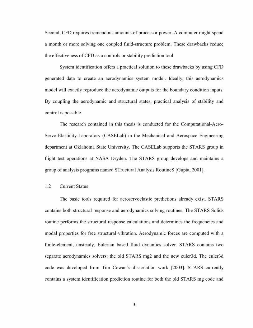
Second, CFD requires tremendous amounts of processor power. A computer might spend
a month or more solving one coupled fluid-structure problem. These drawbacks reduce
the effectiveness of CFD as a controls or stability prediction tool.
System identification offers a practical solution to these drawbacks by using CFD
generated data to create an aerodynamics system model. Ideally, this aerodynamics
model will exactly reproduce the aerodynamic outputs for the boundary condition inputs.
By coupling the aerodynamic and structural states, practical analysis of stability and
control is possible.
The research contained in this thesis is conducted for the Computational-Aero-
Servo-Elasticity-Laboratory (CASELab) in the Mechanical and Aerospace Engineering
department at Oklahoma State University. The CASELab supports the STARS group in
flight test operations at NASA Dryden. The STARS group develops and maintains a
group of analysis programs named STructural Analysis RoutineS [Gupta, 2001].
1.2 Current Status
The basic tools required for aeroservoelastic predictions already exist. STARS
contains both structural response and aerodynamics solving routines. The STARS Solids
routine performs the structural response calculations and determines the frequencies and
modal properties for free structural vibration. Aerodynamic forces are computed with a
finite-element, unsteady, Eulerian based fluid dynamics solver. STARS contains two
separate aerodynamics solvers: the old STARS mg2 and the new euler3d. The euler3d
code was developed from Tim Cowan’s dissertation work [2003]. STARS currently
contains a system identification prediction routine for both the old STARS mg code and

4
the euler3d code. The euler3d system identification routine was ported from the old
STARS code and was not validated.
1.3 Simulation Overview
This section describes the fundamentals of the aeroservoelastic prediction
methodology used in this thesis. The underlying process combines structural and
aerodynamic simulations. These two processes are combined for aeroservoelastic
predictions. The final fundamental process is the system identification or training
methodology.
1.3.1 Structure
The structural simulation determines the time response of the elastic structure. For
typical aeroservoelastic behavior, the structure remains in the linearly elastic region. This
allows for decomposing arbitrary motions into a sum of orthogonal modeshapes, Φ, with
individual modal motions, q. Practically, this means that each structural mode has an
associated shape, mass, stiffness and damping. The second order differential equation for
structural motion in the modeshape reference frame is:
[ ] [ ] [ ] )(tFqKqCqM =++ ΦΦΦ &&&
This allows arbitrary structural motions of complex aerospace vehicles to be simulated by
simple second order ordinary differential equations. The structural response is described
by an array of generalized modeshape displacements rather than describing each
individual point on the structure. For example, the first 4 bending modes of a cantilever
beam are plotted in Figure 1.2. Likewise, the dynamic displacement response of a mode

5
is described by a single number, generalize motion. This is shown for first mode bending
in Figure 1.3.
ModeshapeFrequency
3.516
22.03
61.70
120.9
Figure 1.2 Modeshapes
Phase [deg]
180
90
0
150
120
60
30
GeneralizedMotion
1.00
-1.00
0
0.33
0.66
-0.33
-0.66
Structural Displacement
Figure 1.3 Modeshape Dynamics
A complication arises when external forcing is applied. The overall external
forcing must be reduced to a single generalized force. When an arbitrary pressure
distribution is applied, the effective generalized force on each mode is determined by:
),()()( txPxtF TΦ=
This is essentially the dot produce of the local external force and the modeshape. The
concept is illustrated in Figure 1.4 for a spatially constant force. Thus, the effective force
on a mode is reduced to a single number, generalized force.

6
Modeshape and Applied Force
Generalized Force
2.16
0.53
)()( xPxF ⋅Φ=
0.61
0.84
Figure 1.4 Generalized Forces and Modeshapes
The overall governing equation for the structural motion is the following second order,
constant coefficient differential equation:
[ ] [ ] [ ] ),()( txPxqKqCqM TΦ=++ ΦΦΦ &&&
1.3.2 Aerodynamics
The aerodynamic simulation determines the temporal and spatial characteristics of
a fluid flow. The objective is to determine the local pressures within a specified flow field
subjected to specified boundary conditions. For the CFD analysis presented in this thesis,
the governing fluid dynamics equation is the compressible Euler equation. Unsteady flow
solutions are obtained by a time-marched approach. This requires local iterations to
converge the flow solution at each timestep. Global steps advance the solution in time. A
flow diagram of the CFD solver reproduced from the euler3d development dissertation
[Cowan, 2003] is shown in Figure 1.5.

7
read solver control parameters
read geometry data: COOR, IELM, ISEG, IBEL
compute additional geometry data: G2D/G3D, DM, RBE, WSG, ANOR
read any elastic/dynamic data
set/read initial conditions for UN for t = 0
compute initial aerodynamic loads for t = 0
compute initial structural dynamics state for t = 0
output initial conditions for t = 0
UNO = UN
UN1 = UN
do istp = 1,nstp
advance structural dynamics from t = n to t = n + 1
update ANOR and compute BVEL (transpiration) for t = n + 1
compute local time step, DELT, for each node
do icyc = 1, ncyc
initialize RHS
enforce flow tangency on UN1
add element integrals to RHS
add boundary integrals to RHS
add dissipation to RHS
enforce flow tangency on RHS
UN1 = UN1 – DELT·DM·RHS
enddo
output solution residuals
UN0 = UN
UN = UN1
compute new aerodynamic loads for t = n + 1
output forces and dynamics for t = n + 1
if MOD(istp, nout) = 0, output solution unknowns
enddo
Figure 1.5 CFD Flow Chart [Cowan, 2003]
Unsteady structural boundary conditions are specified from the structural modeshapes, Φ,
using transpiration. Transpiration simulates an actual structural motion with a change in
the boundary normal. The actual CFD grid does not move. Transpiration is illustrated for
a displacement boundary condition in Figure 1.6.
SteadyBoundaryCondition
n̂
n̂
UnsteadyBoundaryCondition
n̂
Actual Boundary Conditions Simulated Boundary Conditionswith Transpiration
Figure 1.6 CFD Boundary Conditions: Actual and Transpiration

8
Integration of the local pressure over the structure allows for calculating the generalized
forces. Aeroservoelastic responses are determined though a loop. The CFD solver
determines generalized forces given generalized motions. The structural solver
determines new generalized motions given the generalized forces. The entire process is
then repeated. This process is stylized in Figure 1.1.
1.3.3 System Identification
The objective of system identification is to determine a system model that predicts
the system dynamics. For this thesis, system identification involves determining
generalized forces from generalized motions. The process is conceptually shown in
Figure 1.7.
Input Known Motion
Excite UnsteadyAerodynamics
Create SystemModel
GeneralizedMotion
GeneralizedForce
System ModelCoefficients
[ ]=ia
System Flow Diagram
Typical Output
Output Data Type
Figure 1.7 System Identification
The basic process is to input a known motion into the aerodynamic system. The CFD
solver uses this input generalized motion to calculate generalized forces. The relationship
between the generalized motions and forces is used to create a system model. Once the
system model is determined, the generalized forces resulting from arbitrary generalized
motion inputs can be found.

9
1.4 Objectives
The objective of this thesis is to improve the current state of linear system
identification techniques for aeroservoelastic predictions. The system under consideration
is multi-input multi-output aerodynamics for use in stability and control analysis.
Limitations and sensitivities with the present prediction method will be identified.
These critical areas will be found by evaluating the current prediction method with
known physics and computational limitations.
Development of improved prediction techniques will follow from the experience
gained. Prediction selection criteria will be developed to evaluate model performance.
These improvements will be implemented and tested.
Finally, the improved prediction methodology will be used for stability and
control analysis of typical aeroservoelastic systems. Results will be compared with the
old methodology. Questions and further research suggestions will be presented.

10
CHAPTER 2
2LITERATURE REVIEW
This chapter examines the literature for unsteady aerodynamics and description
techniques. Some fundamental unsteady aerodynamic theories are reviewed. Then, a
review of relevant system identification literature is given. Next, excitation signal
literature is reviewed. Finally, previous work concerning the development of the
structural, aerodynamic and aeroservoelastic system models is reviewed.
2.1 Unsteady Aerodynamics
A fundamental requirement of aeroservoelastic modeling is determining the
forces caused by unsteady aerodynamics. The boundary condition history specifies the
flow geometry; however, a complication arises because the fluid flow has memory. This
makes determining the forces resulting from unsteady fluid flow significantly more
complex.
The general problem for unsteady aerodynamics is to find a solution that is
consistent with fluid continuity, fluid momentum conservation and the unsteady
boundary conditions. In general, a closed-form solution to arbitrary unsteady flows is not
available.
Closed form simplified solutions to supersonic unsteady flows are available.
Supersonic flows are tremendously simplified because flow influences cannot travel
upstream [Dowell, 1995]. For small perturbations, piston theory provides a simple and
11
reasonably accurate flow prediction methodology [Hunter, 1997]. This solution
methodology is already implemented in STARS.
Closed form subsonic unsteady solutions based on simplified physics are
available when assuming certain conditions. The typical assumptions are inviscid,
irrotational and incompressible flow with a thin airfoil. These assumptions reduce the
solution to an analytic solution, which can be solved for certain restrictive boundary
conditions. The classic Wagner and Theodorsen unsteady solutions result from these
assumptions.
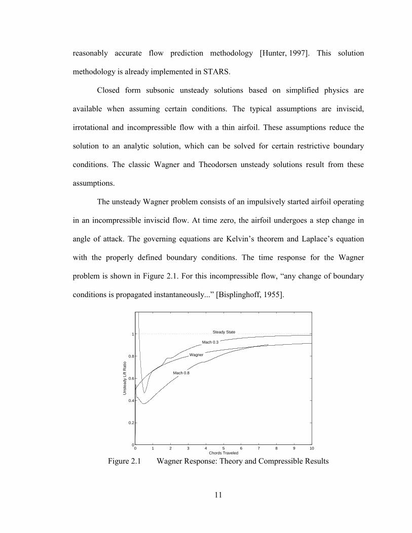
The unsteady Wagner problem consists of an impulsively started airfoil operating
in an incompressible inviscid flow. At time zero, the airfoil undergoes a step change in
angle of attack. The governing equations are Kelvin’s theorem and Laplace’s equation
with the properly defined boundary conditions. The time response for the Wagner
problem is shown in Figure 2.1. For this incompressible flow, “any change of boundary
conditions is propagated instantaneously...” [Bisplinghoff, 1955].
0 1 2 3 4 5 6 7 8 9 100
0.2
0.4
0.6
0.8
1
Chords Traveled
Uns
tead
y Li
ft R
atio
Mach 0.3
Mach 0.8
Steady State
Wagner
Figure 2.1 Wagner Response: Theory and Compressible Results

12
The Wagner problem is not a physically realizable compressible aerodynamic
operation due to the step change in the boundary conditions. A CFD solver can solve the
flow field for this step input; however, the flow solution is not actually the desired step
input response. Parameswaren [1997] describes this situation:
For example, if the airfoil is suddenly exposed to the flow at a different
angle of attack, then the airfoil will also experience an infinite pitch rate.
Then, the response will certainly be a reflection of a step change in
angle of attack as well as an impulsive change in the pitch rate.
Experimentation with the STARS flow solver shows that a “step” angle of attack input
also excites pitch rate and acceleration terms. Figure 2.1 shows the corresponding Mach
0.3 and Mach 0.8 compressible Wagner responses as computed by euler3d. These results
qualitatively agree with the compressible indicial lift response calculated by Bisplinghoff
[1955]. Infinite lift is predicted for the 0+ timestep. This indicates that the Wagner step
input will not properly excite the desired aerodynamic response.
The Theodorsen problem describes the unsteady aerodynamics resulting from an
airfoil undergoing harmonic pitching and plunging motion. The classical derivation is
made in an incompressible inviscid flow [Bisplinghoff, 1955].
The expression for the magnitude of the harmonic lift is:
( ) ( ) )(22 kCbaUhUbbaUhbL ααρπααπρ &&&&&&& −++−+=
The C(k) term is a frequency dependent wake influence term. The parameter k is defined
as a reduced frequency in the following form:
Uck
2ω=

13
The Theodorsen function, C(k), is complex valued and is defined as the following ratio of
Hankel functions:
)()()(
)( )2(0
)2(1
)2(1
kiHkHkHkC
+=
A plot of the Theodorsen function is given in Figure 2.2. For low frequencies, this
form approaches the steady state lift. At high frequencies, the unsteady lift magnitude
approaches one half the steady state lift.
0 0.1 0.2 0.3 0.4 0.5 0.6 0.7 0.8 0.9 1
0.2
0.1
0
0.1
0.10.20.3
0.5
1
2
4
∞ 0
Theodorsen Function, C(k)
Reduced Frequency
U
ck
2
ω=
Real C(k)
Imaginary C(k)
Figure 2.2 Theodorsen Function
It is important to notice that the maximum unsteady phase difference occurs near
a reduced frequency of 0.2. At high and low reduced frequencies, the unsteady
aerodynamic loading is in phase with the motion. This implies that for an airfoil-based
aerodynamic system, the largest phase differences occur at moderately low reduced
frequencies. Destructive aero-structural coupling typically occurs in the moderate to low
reduced frequency range.
The unsteady aerodynamics resulting from arbitrary motion can be described by
combining Fourier theory and the Theodorsen result. The relationship between the time
domain and frequency domain representations of a signal is based on Fourier theory.
Given a generalized motion function f, the lift in the time domain is [Zwillinger, 1996]:

14
∫∞
∞−
⋅−= ωρπρ ω dekfkCUbtfbL ti)()()(2
This implies that a general aerodynamics function will have force components resulting
from both instantaneous motion and lagged wake convection.
2.2 Aerodynamic System Models
This section compares description functions for aerodynamic modeling. There are
many possibilities to choose from. A good overview of the possibilities is given by Ljung
[1987]. Several system models are compared: ARMA, indicial, reduced order modeling
and nonlinear. The basic comparison will be between the ARMA and indicial methods.
Nonlinear methods are only discussed as a comparison to linear methods.
2.2.1 Indicial Methods
Indicial models describe outputs by the convolution of responses and inputs.
These models have output expressions derived from the following continuous time
convolution integral [Chen 1999]:
∫ −=t
dtutgty0
)()()( ττ
The indicial response function is g(t) and the input is u(t). For systems with a single input
parameter, the indicial response is simply the step response. For coupled input systems,
the indicial response becomes significantly more complicated. For a proper indicial
response, the effects of displacement, velocity and the higher order terms must be
decoupled. This can be difficult in aerodynamic training. Additionally, this requires an
indicial response for every proposed input term. For example, Bisplinghoff [1955] shows
that the compressible indicial lift response starts from infinity, which is in contrast to the

15
incompressible Wagner response. The difference is the presence of coupled boundary
conditions. Indicial response functions must be specifically decoupled and trained for
each motion boundary condition. This is a major disadvantage for generic aerodynamic
predictions.
Aerodynamic representation by indicial methods is popular. Cai [2000] used
indicial aerodynamic responses on displacements and velocities for bridge aeroelastic
response calculations. The indicial responses were calculated by fitting to Theodorsen-
based frequency-domain expressions. Cai admits that the indicial response is “very
difficult to measure directly.” Reisenthel [1997] extended the basic indicial response to
account for nonlinear effects in aircraft flight dynamics.
2.2.2 ARMA
The ARMA form consists of a discrete time input-output linear relationship
[Brockwell, 1991]. The basic premise is that the output depends on that previous outputs
and inputs. At the kth timestep, the mathematical representation of the output is the
following:
[ ] [ ]∑∑−
==
−+−=1
01)()()(
nb
ii
na
ii ikxBikyAky
The system’s input response is described by:
[ ]∑−
=
−1
0)(
nb
ii ikxB
The system’s internal response is described by:
[ ]∑=
−na
ii ikyA
1)(

16
The ARMA form directly corresponds to a discrete form of an ODE. The general
form for an ARMA model can be written as a p-order output and a q-order input.
∑∑ −=− )()( qtxbptya qp
A general ODE is written as an m-order output and an n-order input.
( ) ( )∑∑ = nn
mm xdyc
Expanding the ODE expression for a 4 by 3 order yields the following result.
( ) ( ) ( ) ( ) ( ) ( ) ( )22
11
00
33
22
11
00 ycycycycycycyc ++=+++
Using a Taylor’s series approximation to derivatives yields the following finite difference
expressions.
( )
( )
( )t
kyy
tkykyy
kyy
∆+≈
∆−−≈
=
L)(
)1()()(
2
1
0
( )
( )
( )t
kxx
tkxkxx
kxx
∆+≈
∆−−≈
=
L)(
)1()()(
2
1
0
Substituting in these finite difference approximations yields the following expression.
LLLLLL +−
+
∆−
+
+
∆+=+−
+
∆−
+
+
∆+ )1()()1()( 11
011
0 kxtdkx
tddky
tcky
tcc
This is exactly the ARMA form.
The ARMA form assumes a linear relationship between the current output and the
previous states. This form allows for simplified system identification. The following
expression shows the overall linear expression:
}OutputCurrent InputsCurrent andPast
11
Outputs Previous
)()1()1()()()()1(M
44444444444 844444444444 76
MLM
LLL4444 84444 76
M
L tyBAnbtxnbtxtxtxnatyty
i
inrnr =
⋅
−−−−−−
In the general case, this expression reduces to the following linear algebra form:

17
[ ] bxArr =
This form can be solved through any of a number of linear algebra methodologies.
The advantages of ARMA are tremendous. First, ARMA allows for an intuitive
system identification implementation. The model coefficients can directly be determined
from linear system theory. Second, the ARMA form is easily transformed to a state space
form consistent with aerodynamic prediction requirements. Third, ARMA can properly
model MIMO systems without additional complications.
A particular disadvantage of ARMA is determining a sufficient model order. This
model order problem causes particular difficulties for long lag systems. Multiple papers
give model order estimation guidelines; however, most are based on difficult to
implement stochastic frameworks. Gevers [1986] derives the McMillan degree, order, of
an ARMA system. Gevers states:
These [monic ARMA] models can only represent systems whose
McMillan degree is a multiple of the number of outputs. In all other
cases they will tend to produce estimated models of higher order than
the true system.
This result has not been discussed in the literature with respect to aerodynamic modeling.
2.2.3 Nonlinear
Nonlinear description models allow for advanced predictions for complex
systems. The number of methods, which are available for nonlinear descriptions, is
immense. These methods allow for advanced predictions by capturing more of the
underlying physics. For aerodynamics, nonlinear analysis is needed for limit cycle
predictions as well as high angle of attack and other common flow regimes. Hamel

18
[1996] gives examples of nonlinear unsteady flow models and their performance results.
Theoretically, a nonlinear description should have no small-perturbation limitations. In
practice, assuming a nonlinear description complicates the system identification process.
Nonlinear analysis is already computationally expensive. Additionally, the nonlinear
identification process requires data throughout the desired system prediction operational
area [Reisenthel, 1997]. If the training does not excite the dominant nonlinearities, then
the identification will not determine an accurate system model. This may require a
training length an order of magnitude longer. A useful excitation will need information at
all expected motion magnitudes. Depending on the system complexity, the excitation
may need exotic motion specifications to properly account for the nonlinear system
dynamics. Some of these motion combinations are difficult to reach in a consistent
manner. Another disadvantage is the loss of traditional linear system theory. This implies
that the entire identification and evaluation process becomes time response dominated.
All response evaluations will be based on how the system reacts in time. This forces
system identification into more of a black-box experiment rather than a system property
evaluation. Prematurely switching to nonlinear models appears to inhibit the
understanding and physical insights allowed by linear system identification. For many
aerostructural problems, the fundamentals can be captured by a linear system. As Dowell
[1996] points out:
One of the pleasant ironies for the aeroelastician has been that such
calculations have revealed that a linear dynamic model perturbed from a
nonlinear static or steady flow model which includes shock waves is
sufficiently accurate for describing many flutter phenomena.

19
A related nonlinear description technique is reduced-order-modeling. This
technique seeks to reconstruct the unsteady flow properties through an eigenvalue
analysis of the entire flow field. Not surprisingly, ROM is tremendously computationally
expensive. Also, ROM does not result in a direct state space form for aerodynamic
forces; the resulting pressure must be integrated over the modeshape. ROM does not
appear to be a general method for aerodynamic predictions due to jump changes in
aerodynamic flow solutions [Raveh, 2001] [Reisenthel, 1997]. Florea [2000] found that
ROM gave excellent flow predictions even at transonic Mach numbers. Florea found that
a 2D NACA 0012 airfoil at Mach 0.1 required 10 eigenvalues while the Mach 0.85 case
required approximately 310 eigenvalues, which presented further computational
difficulties.
2.3 System Identification Methodologies
The objective of system identification is to fit a system model to measured data.
Better system models result from more data; however, this effectively creates an
overdetermined system, which has more data than equations. Björck [1996] states, “... the
solution which minimizes a weighted sum of the squares of the residual is optimal in a
certain sense.” The system model as presented in the previous section can be reduced to a
general linear equation form as shown below:
[ ] bxArr =
Direct solutions by the traditional linear algebra techniques will not be successful
for multiple reasons. First, [ ]A is not square; a traditional inverse does not exist. Second,
the condition of [ ]A is typically such that the numerical routine will create significant
errors. A better solution technique is to switch to a methodology capable of handling
20
these difficulties. Iteration and Singular Value Decomposition appear to be the most
commonly used numerical routines for linear system identification. The current STARS
system identification method uses SVD.
Iteration consists of solving a particular equation with successive approximations.
The routine consists of iteration until the solution is “good” enough. Björck shows that
iteration is “attractive” for sparse matrices due to storage requirements, convergence rate
and solution speed. Improved solution speed typically results from a compressed matrix
form [Björck, 1996]. Multiple iterative solution methods exist; picking one method
involves selecting among many schemes, pre-conditioners and factorizations. Iteration
also allows for advanced solutions based on external constraints and other non-typical
least squares formulations. The primary disadvantage of iteration schemes is their
consistency. Björck [1996] notes:
The main weakness of iterative methods is their poor robustness and
often narrow range of applicability. Often, a particular iterative solver
may be found to be very efficient for a specific class of problems, but if
used for other cases it may be excessively slow or break down.
This is a significant disadvantage for system identification.
Singular value decomposition is a linear algebra technique for reducing any
matrix to two basis matrices and one diagonal matrix. The SVD expression form for an
arbitrary matrix A is given as [Press, 1992]:
SVUA T=
The U and V matrices are the basis matrices; the diagonal S matrix contains the singular
values. The pseudoinverse of A is [Press, 1992]:

21
TVWUA =+
W is the inverse of each diagonal term in the S matrix. Solution simplifications are
possible by dropping small singular values. Press [1992] proposed using this
simplification to determine the dominant solution structure.
The advantages of SVD are significant. SVD always finds a least-square solution.
Press says, “SVD can be significantly slower than solving the normal equations;
however, its great advantage, that it cannot fail, more than makes up for the speed
disadvantage”. Another advantage is that the SVD data structure shows solution
information based on the singular values. Björck [1996] shows that “perturbations of the
elements of a matrix produce perturbations of the same, or smaller, magnitude in the
singular values.” The primary disadvantage of SVD is the computational expense,
especially for large problems. Also, small singular values are often corrupted by machine
precision errors.
Variants of the SVD routine exist for specialized applications. Traditional SVD
provides a “most” least-square solution [Press, 1992] based on the Frobenius norm, L2.
The Frobenius norm is defined as:
∑= 2
2 iaA
Others have demonstrated that the traditional least-squares formulation does not
always yield the best solution. A simple modification to the traditional SVD routine is the
Total Least Squares. Deprettere [1988] shows that the method “is appropriate when there
are errors in both the observation vector b and the data matrix a...” Björck [1996] states
that Van Huffel [1991] found 10 to 15 percent improvements in solution quality with
Total Least Squares over Least Squares. The solution quality criteria were not reported.

22
Björck [1996] also show a methodology for converting Total Least Squares problems to
Least Squares problems.
Subspace identification techniques are popular. Moonen [1990] proposed a
“quotient SVD” for system identification with non-white noise. The solution
methodology reduced to performing SVD twice. The additional SVD calculation
determines an input-output data subset with the greatest signal to noise ratio. The results
show that QSVD gave improved predictions for small signal to noise ratios. Overschee
[1993] uses a similar method to compute a system model based on a Kalman filter, which
was based on the raw input-output data. The approach is significantly more complicated
than the traditional SVD approach. Additionally, the approach appeared to give more
precise solution but with a significantly wider error distribution when compared to a
traditional approach.
For computer vision applications, Irani [2002] found that including uncertainty
into the SVD formulation significantly improved shape and motion predictions.
Directional uncertainty estimates were included through a covariance weighted scheme,
which minimized the Mahalanobis distance rather than the Frobenius norm. Mahalanobis
distance effectively assigns variable penalty weighting factors to each orthogonal solution
directions. This means that errors in the x direction, for example, are penalized more than
errors in the y direction. The disadvantage of this formulation is that useful penalty
weighting factors are needed. Determining the weighting factors can become complicated
for multi-dimensional problems. For Irani, a useful covariance data structure resulted
from the physical restriction of four dimensions: space and time.

23
2.4 Input Training Signals
Successful system identification requires selecting a sufficiently good input
training signal. Selection techniques are typically based on estimated system
characteristics. Typically, these criteria are only mathematical in form and are not tested
for practicality and sensitivity. This section will review basic input signal forms and
examine their performance for aerodynamic system identification in the time domain.
The literature provides abundant information on signal design and system
identification techniques. However, most input signals are designed and evaluated for
frequency domain identification. While the fundamental requirements for the time
domain are similar, identification in the time domain has some subtle differences. Any
input signal can be used for time domain identification [Miller, 1986]; however, the
quality of the resulting model will reflect the input signal quality. While basic system
predictions may be possible with simple system models and arbitrary input signals,
system models that are used for controls need good resolution and accuracy in describing
the system. The input signal needs to take into account the overall system processes to
avoid over-driving or forcing non-linearity [Braun, 2002]. Historically, the binary signal,
the frequency sweep and the multisine are the most commonly used signals for system
identification. For flight-testing, the multisine and the binary signals are typically the
most common [McCormack, 1995]. The binary signal, the frequency sweep and the
multisine will be investigated.
Binary signals consist of a series of pulses arranged for a specified frequency
spectrum. Unfortunately, the binary signal frequency spectrum contains unexcited areas
that can only be removed by adding significant length to the signal [Schoukens, 1988]. In

24
this regard, binary signals are similar to noise or stochastic signals [Schoukens, 1988].
Random noise signals could be considered as binary signals with variable pulse heights.
Schoukens [1988] shows that random noise does not automatically average out system
nonlinearities. A binary signal, the 3211 multistep, is one of the most commonly used
flight-test signals [Miller, 1986]. This may be in part because the multistep is easy to
implement and contains a relatively simple functional form.
Frequency sweeps are generated from sinusoidal functions with a smoothly
varying frequency. This has the advantage of exciting all frequencies within a specified
bandwidth. Linear frequency sweeps are commonly referred to as chirps. Frequency
sweep are common in the flight test community [Miller, 1986]. However, one
disadvantage of a sweep is poor low-frequency performance [Young, 1990][Brenner,
1997]. Investigations into improving chirp frequency response are not common; most
investigators switch to multisines to improve low frequency response. Numerical
difficulties [Zwillinger, 1996] associated with advanced frequency sweep forms are,
possibly, responsible for limited development. Another disadvantage is that the frequency
sweep can overexcite the structure and cause ``critical flight incidences’’ [Miller, 1986].
Sweeping through a structural or aeroelastic resonance frequency allows for the
possibility of unintentionally overexciting the structure. Because the sweep advances in
frequency, the structure may already have dangerous motion amplitudes even before the
actual resonance frequency.
The classic multisine signal is the Schroeder sweep [Schroeder, 1970]. Variable-
phase discrete frequencies are added to yield an arbitrary PSD across a specified
bandwidth. The Schroeder sweep visually resembles a frequency sweep during part of the

25
overall harmonic signal [Van Der Ouderaa, 1988]. Algorithms for minimizing the
multisine peak factor are common [Braun, 2002] [Van Der Ouderaa, 1988] [Mehra, Dec.
1974] [Mehra, June 1974]. For overall performance, Young and Patton [1990] found that
for a specific helicopter identification problem, a multisine gave slightly better results
than the corresponding frequency sweep. This improvement appeared to be due to
improved low frequency excitation with the multisine. Simon [2000] found that the
Schroeder sweep is sensitive to the signal excitation length.
2.5 Model Quality
Model quality evaluations are necessary to ensure the system identification
process correctly modeled the relevant physics. An excellent criterion exists for
statistically based models [Akaike, 1974]; however, it is not quite as intuitive for ARMA
based models. Ninness [1995] surveys model quality estimation methodologies for both
frequency domain and time domain identification. The underlying emphasis is model
selection and identification for robust control. Ninness indicates that deterministic
identification is preferred over stochastic identification for robust control. Mäkilä [2003]
provides a methodology for determining the size of unmodeled dynamics between a
linear system and the actual system. The paper proposes using the Fréchet derivative to
evaluate mildly nonlinear systems. Model quality is affected by the discrete time
timestep. “It is well known” [Worden, 1995] that over-sampling leads to system
identification difficulties. Åström [1969] shows that an optimal sampling rate occurs for
simple system identification. As expected, Åström found that the model quality
degradation is worse for undersampling than for oversampling.

26
2.6 Aerodynamic and Structural System Representations
The aeroelastic predictions are based on aerodynamic and structural models. This
section will discuss the formulation of these models. These derivations were created by
Cowan [2001].
2.6.1 Structural Model
Structural motion is decomposed into orthogonal modes. The overall structural
response becomes a second order ordinary differential equation with constant structural
coefficients M, C and K and an arbitrary modal forcing function F:
[ ] [ ] [ ] FqKqCqM =++ &&&
Two structural states are required to represent this system. Each state contains the
displacement and velocity of each mode. Mathematically, the structural state vector is
given as the following:
[ ]Ts qqx &r =
Decomposing the second order differential equation into two first order equations yields
the following state space form:
[ ] [ ][ ] [ ] )()()(
)()()(tFDtxCtqtFBtxAtx
sss
ssss
+=+=&
The state space parameters As, Bs, Cs and Ds are determined from the structural
parameters by the following matrix form:
[ ] [ ] [ ][ ] [ ] [ ] [ ]
−−
= −− CMKMI
As 11
0 [ ] [ ]
[ ]
= −1
0M
Bs
[ ] [ ] [ ][ ]0ICs = [ ] [ ]0=sD

27
The above continuous state space form is transformed to a discrete state space
form with the matrix exponential. This form is based on an evenly spaced discrete
timestep. The state space form becomes the following at the kth time step:
[ ] [ ][ ] [ ] )()()(
)()()1(kFDkxCkq
kFHkxGkx
sss
ssss
+=+=+
The state space parameters Gs, Hs, Cs and Ds result from the appropriate discrete
transformations:
[ ][ ] [ ] [ ]( )[ ] [ ]ssss
dtAs
BAIGH
eG1−
⋅
−=
=
The structural response is now represented in a discrete state space form appropriate for
connecting as an input-output system.
2.6.2 Aerodynamic Model
The aerodynamics are represented as a linear ARMA state space model.
Constructing the aerodynamic system model requires storing previous aerodynamic
forces f and inputs q . The system model state vector is the following:
+−
−−
−
=
)1(
)1()(
)1(
)(
nbkq
kqnakf
kf
kxa
M
M
In a discrete state space form, the aerodynamic state space form is the following. This
aerodynamic model was composed in discrete time, so a continuous-discrete conversion
is not necessary as it was in the structural case:

28
[ ] [ ][ ] [ ] 0)()()(
)()()1(fkqDkxCkf
kqHkxGkx
aaaT
aaa
++=+=+
The following state space parameters Ga, Ha, Ca and Da result from expanding the ARMA
state space model in terms of the state space vector )(kxa :
[ ]
[ ] [ ] [ ] [ ] [ ] [ ] [ ] [ ][ ] [ ] [ ] [ ] [ ] [ ] [ ] [ ][ ] [ ] [ ] [ ] [ ] [ ] [ ] [ ]
[ ] [ ] [ ] [ ] [ ] [ ] [ ] [ ][ ] [ ] [ ] [ ] [ ] [ ] [ ] [ ][ ] [ ] [ ] [ ] [ ] [ ] [ ] [ ][ ] [ ] [ ] [ ] [ ] [ ] [ ] [ ]
[ ] [ ] [ ] [ ] [ ] [ ] [ ] [ ]
=
−−−
0000000
00000000000000000000000000000
00000000000000
1221121
I
II
I
II
BBBBAAAA
G
nbnbnana
a
LL
MMOMMMMOMM
LL
LL
LL
LL
MMOMMMMOMM
LL
LL
LL
[ ]
[ ][ ][ ]
[ ][ ][ ][ ]
[ ]
=
0
00
0
00
0
M
M
I
B
H a
[ ] [ ] [ ] [ ] [ ] [ ] [ ] [ ] [ ][ ]1221121 −−−= nbnbnanaa BBBBAAAAC LL [ ] [ ]0BDa =
2.6.3 Aeroelastic Model
The above development of discrete time structural and aerodynamic system
models is continued by joining the models. The coupled system diagram is given in
Figure 2.3.
Structure
Aerof̂
q
∞q
f
TfIf+
+
Figure 2.3 Coupled Aeroelastic System
The resulting state space model describes the system’s coupled aeroelastic response. The
overall structural response vector is given by )(kq . The aerodynamic forces are scaled by

29
the dynamic pressure ∞q . The system model contains an impulsive forcing function via
the If input.
Substitution yields the following system model:
[ ][ ][ ]
=
+
+
+=
++
∞∞∞
)()(
0)(
0
ˆ
0)()(
)1()1( 0
kxkx
Ckq
fHqfH
kxkx
GCHCHqCDHqG
kxkx
a
ss
sI
s
a
s
asa
assass
a
s
This coupled form of the combined aerodynamic and structural models is
sufficient for determining aeroelastic free response characteristics. A free response
simulation consists of matrix multiplication and state vector storage. Matrix operations
are orders of magnitude faster than an unsteady CFD solution. The system stability
boundary can be found in the time domain by successive bounding of stable-unstable
dynamic pressures.
The intrinsic system stability is determined from the plant matrix. The plant
matrix is a function of the structure with the submatrices Gs, Hs and Cs and a function of
the aerodynamics with the submatrices Da, Ca, Ha and q∞. The plant matrix shown below
has dimensions ( )( ) ( )( )11 ++⋅×++⋅ nanbnrnanbnr :
+ ∞∞
asa
assass
GCHCHqCDHqG
Locations of eigenvalues in the z plane with respect to the unit circle indicate the overall
stability of the system. There are ( )1++⋅ nanbnr eigenvalues for a na-nb model with nr
modes.
30
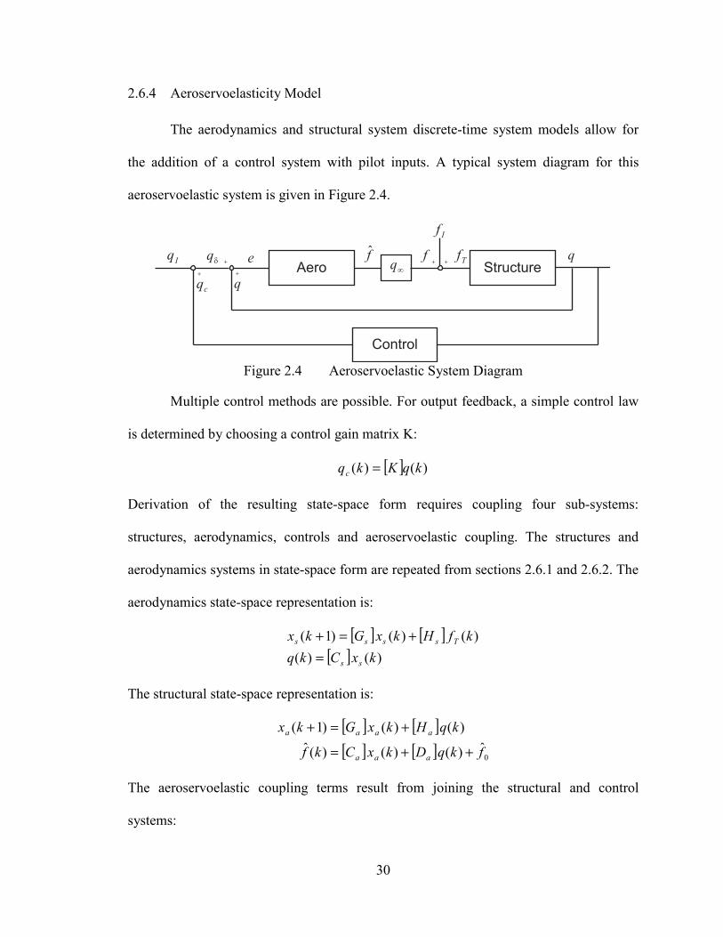
2.6.4 Aeroservoelasticity Model
The aerodynamics and structural system discrete-time system models allow for
the addition of a control system with pilot inputs. A typical system diagram for this
aeroservoelastic system is given in Figure 2.4.
StructureAerof̂ q
∞qf Tf
If
++
q
eδq +
+
Control
cq+
Iq
Figure 2.4 Aeroservoelastic System Diagram
Multiple control methods are possible. For output feedback, a simple control law
is determined by choosing a control gain matrix K:
[ ] )()( kqKkqc =
Derivation of the resulting state-space form requires coupling four sub-systems:
structures, aerodynamics, controls and aeroservoelastic coupling. The structures and
aerodynamics systems in state-space form are repeated from sections 2.6.1 and 2.6.2. The
aerodynamics state-space representation is:
[ ] [ ][ ] )()(
)()()1(kxCkq
kfHkxGkx
ss
Tssss
=+=+
The structural state-space representation is:
[ ] [ ][ ] [ ] 0
ˆ)()()(ˆ)()()1(
fkqDkxCkf
kqHkxGkx
aaa
aaaa
++=
+=+
The aeroservoelastic coupling terms result from joining the structural and control
systems:

31
qqeqqq
fqf
fff
cI
IT
+=+=
=
+=
∞
δ
δ
ˆ
The derivation of the aeroservoelastic state-space form is as follows. The aeroservoelastic
coupling terms are added into the aerodynamics:
0ˆ)()()(ˆ
)()()1(
fkeDkxCkf
keHkxGkx
aaa
aaaa
++=
+=+
Next, the structural outputs are added to the resultant aerodynamics:
( )( ) 0
ˆ)()()()()(ˆ)()()()()1(
fkxCkqkqDkxCkf
kxCkqkqHkxGkx
sscIaaa
sscIaaaa
++++=
+++=+
The control algorithm is added to the aerodynamics:
( )( ) 0
ˆ)()()()()(ˆ)()()()()1(
fkxCkxKCkqDkxCkf
kxCkxKCkqHkxGkx
ssssIaaa
ssssIaaaa
++++=
+++=+
Next, like terms are collected:
[ ][ ] 0
ˆ)()(I)()(ˆ)()(I)()1(
fkqDkxCKDkxCkf
kqHkxCKHkxGkx
Iassaaa
Iassaaaa
++++=
+++=+
Now, the coupling terms are added to the structural state-space form:
( ))()(ˆ)()1( kfkfqHkxGkx Issss ++=+ ∞
The aerodynamic system is combined with the structural system, and like terms are
collected:
[ ]( )Iss
Iasaasssasss
fHfHq
kqDHqkxCHqkxCKDHqGkx
++
++++=+
∞
∞∞∞
0̂
)()()(I)1(
Finally, the resultant aerodynamics and structural forms are combined into a single state-
space form:

32
[ ][ ]
[ ][ ][ ]
=
+
+
+
+
++=
++ ∞∞∞∞
)()(
0)(
ˆ00)(
)(I
I)1()1(
0
kxkx
Ckq
fHq
qH
DHqf
Hkxkx
GCKHCHqCKDHqG
kxkx
a
ss
sI
a
asI
s
a
s
asa
assass
a
s
This form is sufficient for aeroservoelastic predictions in the time domain. Again, the
plant matrix can be evaluated for eigenvalue placement.

33
CHAPTER 3:
3METHODOLOGY
In this chapter, techniques for improved aeroservoelastic predictions are
developed and tested. This chapter focuses on system models, training methods,
excitation signals, performance evaluation criteria and STARS implementation.
3.1 Aerodynamics System Model
The fundamental concepts of unsteady aerodynamics were used to develop a
generalized and sufficiently complex aerodynamic representation form. This required
determining the fundamental requirements needed for aerodynamic predictions of
aeroservoelastic systems.
3.1.1 CFD Solver
The objective of creating the aerodynamic system model is to replace the slow
CFD solver with a faster aerodynamics representation. The goal is to represent an
arbitrary CFD input-output relationship with an aerodynamic system model. In a general
sense, the source of the input and output is irrelevant, only the system representation
matters. CFD verification and validation remains with the CFD developer. The primary
function of the CFD solver for this thesis is to provide input-output vector pairs. The
CFD solution does not need to represent reality. However, because the CFD solver does
represent an actual physical system, the overwhelming problem of designing a general

34
system model is reduced. Regardless, the system model structure needs to be consistent
with the CFD solver. A review of the euler3d CFD solver’s solution structure is required.
Aerodynamic solutions are determined through time marching of a flow solver
with structural boundary conditions. Boundary conditions are specified through each
element’s displacement and velocity.
Structural response is determined through a discrete time representation of state
and input responses. In continuous time state-space form, the structural state matrices are
formed from the mass, damping and stiffness. When converted to a discrete time
representation, the state transition expression becomes the following:
[ ] [ ][ ] [ ] )()()(
)()()(tFDtxCtqtFBtxAtx
sss
ssss
+=+=&
It is important to note that the representation updates the state vector simultaneously.
3.1.2 Aerodynamic Specific Requirements
Aerodynamic systems have unique requirements when compared to other
systems. Together, these requirements force the reevaluation of common system
modeling techniques.
Aerodynamic systems have input and output dynamics. Fluids have memory of
both motion and flow geometries. This creates a situation where both motion and flow
must be adequately excited to capture the governing physics. Not exciting both
geometries will bias the ARMA model towards unrealistic coefficients for the motion and
force terms. These fluid geometries often have vastly different time-scales. Wake
convection off a body occurs at the free stream velocity, and wave propagation occurs at
sonic velocity. Worse still, wave propagation at transonic Mach numbers has vastly

35
different upstream and downstream clearing times. The aerodynamic modeling technique
must excite these dominant terms.
Aerodynamic systems have practical limitations on motion forms and magnitudes.
Exceeding these limitations places the input-output physics outside the linear regime. For
motion magnitudes, flow separation often effectively determines the linear limitations.
Additional limitations are placed on motion forms due to restrictions on starting and
ending input conditions. Any motion should begin from a steady state aerodynamic
solution to prevent generating unwanted impulsive transients. Steady state implies that
the entire flow field is constant. Steady forces are necessary but not sufficient for a steady
state condition.
Another requirement is that the aerodynamic solution and the boundary conditions
are consistent in a discrete time sense. This requirement becomes more critical with the
current displacement-based ARMA formulation. The training signal needs the same
motion characteristics that the coupled CFD solver uses.
Performance requirements for aeroelastic systems are significantly stricter than
the typical system identification requirements. The aeroelastic geometries under
consideration often operate over wide ranges of dynamic pressure. More seriously, the
prediction point of interest is often the system stability point. As Cowan [2003] found,
stability predictions are sensitive to solution technique.
3.1.3 Objective Function
This section describes unsteady aerodynamics as a generalized objective function.
It seeks to compare the unsteady forms and to select a viable representation, which will
be usable for later description-function selection.

36
Unsteady aerodynamics are complicated. Selecting an objective function based on
a linear representation is not trivial. Determining an objective function directly from a
fluid flow governing equation is just not possible.
The first step in selecting an objective function is to select the physics of the
unsteady flow that should be modeled. An initial selection criterion is to discard any
physics that are not included in the CFD solution. Since the CFD solver is an inviscid
Eulerian solver, this removes non-linear effects due to viscosity and fluid particle
tracking. Another selection criterion results from the use of structural modes for
aerodynamic boundary conditions. This allows only tracking the modal forces and
motions in lieu of tracking the entire flow solution. Now, the aerodynamic modeling
requirements are reduced to a MIMO system for predicting time marched modal forces.
Next, additional assumptions are placed on the system via the expected
magnitudes and forms of the inputs and outputs. The aerodynamic system may have a
static offset; this is easily removed. For most analytic solutions, including aerodynamics,
the residuals remaining, after assuming a strictly linear relationship between current
inputs and outputs, become sufficiently small for small enough inputs. However, this is
an unusually restrictive assumption. Further assumptions need to be based on unsteady
aerodynamic theory.
A review of unsteady aerodynamic theory with respect to input-output
relationships assists in determining a representative objective function. Reviewing the
Theodorsen solution to a harmonically moving airfoil shows that a frequency dependent
phase shift occurs for the non-circulatory portion of the lift. The Theodorsen solution also
indicates that motion displacement, velocity, and acceleration are included in

37
incompressible unsteady aerodynamics. From the wave equation for compressible flow,
additional unsteady effects will occur due to wave propagation resulting from changes in
boundary conditions and vorticity-boundary interactions. Complicating these effects is
that the waves themselves are affected by compressibility. For small amplitude motions
around a mean operating condition, the wave magnitudes are small. A final unsteady
effect occurs due to time lagged responses between two separated bodies. Time lags
occur at wave, potential and convective time scales. From system theory, pure time lags
result in distributed systems. That is, the continuous time transfer function is irrational
[Chen, 1999]. Further investigations yield even further complexities; however, it is fair to
say that the objective function needs to capture magnitude and phase changes with
frequency and also needs to capture pure time lags.
The function should model the dominant flow physics with a linear relationship in
the differential equation sense. Selecting a function based on an m by n order differential
equation provides an initial starting point. The following form is proposed:
)()( )()( delaysxxxxxcdelaysfffff nm ++++++=+++++ L&&&&&&L
This form captures the frequency dependent magnitudes and phases as well as any delay
terms. Additionally, the input dynamics and the output dynamics are observable within
the function.
3.1.4 Description Function Selection
The ARMA formulation is retained as the description function. The ARMA
formulation is already implemented in STARS.
The ARMA form allows for arbitrary high order descriptions through discrete
derivative approximations. The literature review indicated that the indicial forms were

38
not capable of properly modeling the boundary conditions. It was shown that the ARMA
formulation is capable of directly relating a continuous time ODE to a discrete form.
The ARMA form allows for both input and output dynamics. Correctly modeling
both the input and output dynamics is important as shown with the Theodorsen arbitrary
motion derivation. It appears that sensitivities in the current ARMA form are coming
primarily from excitation signal sensitivities.
In summary, the ARMA form allows for aerodynamic prediction. The ARMA
form is retained as the system model description function.
3.1.5 ARMA Realizations and Canonical Forms
There are an infinite number of realizations to describe an ARMA model. Each
form can be expressed as another through a specific transformation. The flow diagram for
the classical ARMA description is shown in Figure 3.1. The ai and bi terms are switched
when compared to the traditional ARMA naming convention. This form corresponds with
the formulation given in section 2.6.2. The past inputs and outputs are stored as separate
states.
One possible canonical ARMA form is shown in Figure 3.2. This formulation has
the past input/output information stored as one state, w(k). This form gives the advantage
of fewer states with the disadvantage of non-intuitive states. The reduction in the state
vector size is the minimum value of either na or nb.

39
Figure 3.1 Classical ARMA Form [Boziac, 1979]
Figure 3.2 Canonic ARMA Form [Boziac, 1979]
The state space representation for the canonical form is derived below. From
Figure 3.2, a logical state vector would be:
−
−−
=
)(
)2()1(
)(
nakw
kwkw
kxaM
A state update expression can be realized from Figure 3.2. However, it should be noticed
that Figure 3.2 swaps the ai and bi coefficients when compared to the traditional ARMA
convention used in this thesis. After substitution, the following state update and output
expressions are determined as the following:
)()()1( kxHkxGkx aaaa +=+
)()()(ˆ kxDkxCkf aaa +=
The canonical state matrices are:
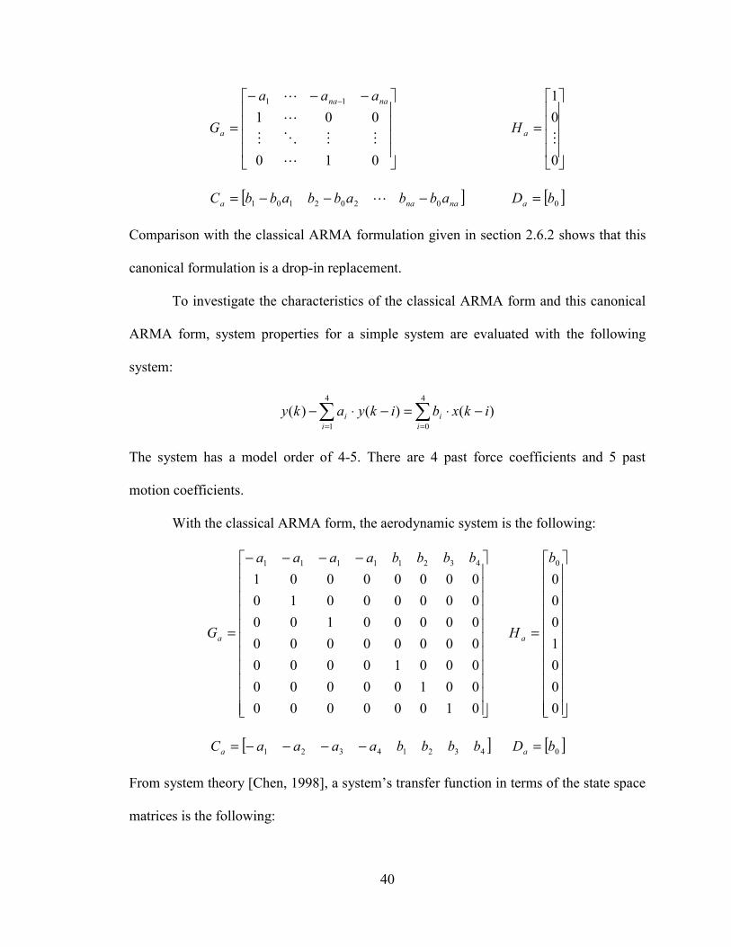
40
−−−
=
−
010
00111
L
MMOM
L
L nana
a
aaa
G
=
0
01
MaH
[ ]nanaa abbabbabbC 0202101 −−−= L [ ]0bDa =
Comparison with the classical ARMA formulation given in section 2.6.2 shows that this
canonical formulation is a drop-in replacement.
To investigate the characteristics of the classical ARMA form and this canonical
ARMA form, system properties for a simple system are evaluated with the following
system:
∑∑==
−⋅=−⋅−4
0
4
1)()()(
ii
ii ikxbikyaky
The system has a model order of 4-5. There are 4 past force coefficients and 5 past
motion coefficients.
With the classical ARMA form, the aerodynamic system is the following:
−−−−
=
0100000000100000000100000000000000000100000000100000000143211111 bbbbaaaa
Ga
=
00010000b
H a
[ ]43214321 bbbbaaaaCa −−−−= [ ]0bDa =
From system theory [Chen, 1998], a system’s transfer function in terms of the state space
matrices is the following:

41
( ) DBAsICsG +−= −1)(
Thus, the investigated system has the following transfer function, which is identical to the
ARMA transfer function given in the previous section:
41
32
23
14
41
32
23
14
0)(azazazazbzbzbzbzbsG
++++++++
=
The canonical ARMA form is investigated next. The following state space
matrices are determined:
−−−−
=
010000100001
4321 aaaa
Ga
=
0001
aH
[ ]404303202101 abbabbabbabbCa −−−−= 0bDa =
Again, the transfer function exactly matches ARMA theory:
41
32
23
14
41
32
23
14
0)(azazazazbzbzbzbzbsG
++++++++
=
A slightly subtle result occurs when the eigenvalues of the classical aerodynamic
plant matrix are determined. The nb terms only contribute to the zero valued eigenvalues.
As a result, the classical and canonical forms contain the same eigenvalues.
The transfer functions for the classical, canonical and theoretical ARMA forms
are identical. For memory usage, the canonical form is preferred because the number of
system states is reduced to the maximum number of states of either the output AR terms
or the input MA terms. For eigenvalue analysis, the canonical form is preferred because
the plant matrix contains fewer terms. However, a major advantage that the classical form
offers is an intuitive state vector. The canonical state vector contains non-intuitive

42
transformed states. The output matrix Ca for the canonical form displays the decreasing
influence of past states in a more intuitive manner than the classical ARMA form.
3.1.6 ARMA Model Transfer Function
Describing the ARMA model as a discrete time filter provides another viewpoint
of the ARMA performance characteristics. From Boziac [1979], the z transfer function
for an ARMA model with model order na-nb is the following:
∑
∑
=
−
−
=
−
+= na
m
mm
nb
n
nn
za
zbzH
1
1
0
1)(
The ARMA model coefficients directly specify the transfer function coefficients.
3.1.7 ARMA Pathology
The ARMA system form is complex enough to allow strange, tricky and
inconsistent behavior for certain conditions. This section describes a few of these non-
intuitive situations, which might be useful.
3.1.7.1 Non-Consistent Training
An ARMA model is capable of describing a wide range of systems; however, the
model quality and coefficient form depend on the input training conditions. With the
current form, only input displacements are correlated with outputs. Training with a
velocity and no resulting displacement will associate the dynamics solely with the past
forces. The only terms that should be non-zero are the past force coefficients, nb terms.
This situation is more common than typically thought. If the motion update expression

43
does not update both displacement and velocity states simultaneously, an off-by-one-
timestep problem can excite this non-consistent training error.
There is a specific case where non-consistent training could be advantageous.
Combining inconsistent boundary conditions with an ARMA model that captures both
boundary conditions would allow training for each boundary condition for each mode.
This further decoupling of aerodynamics might yield better models; however, significant
challenges would result from combining all of the boundary condition models together
for each mode. Additionally, the ARMA form would require extra states to accommodate
the two boundary conditions. Combining the states together in a physically consistent
manner is not trivial. To examine this training method, an initial test was conducted by
adding a single “current” velocity state to the ARMA formulation. Velocity information
is determined from displacement data, so a possible half-timestep error is possible with
the displacement only ARMA form. However, the resulting models for the single velocity
addition were not significantly better.
3.1.7.2 Second Order Accurate Forces
Through a simple modification of the output matrix for the ARMA system, the
output forces can be described by a second order accurate description. The general
second order description for current force is:
)2()1()(2 21
23
2 −+−−= nfnfnff nd
Understanding that the ARMA model structure contains previous forces allows for the
introduction of the second order correction terms directly into the ARMA output matrix
structure. The general non-dimensional force is:
0)()(ˆ fkqDkxCf aaaa ++= .

44
Adding the 2nd order corrections terms gives the following force equation:
0221
123 )()()()(2ˆ fkqDkxSkxSkxCf aaaaaa +++−=
The S correction terms are:
[ ] [ ] [ ][ ][ ] [ ] [ ][ ]00
00
1
1
L
L
ISIS
==
Thus, the overall system output matrix is:
[ ] [ ] [ ] [ ] [ ] [ ] [ ] [ ] [ ][ ]1221141
243
22 −−−+−= nbnbnanaa BBBBAAIAIAC LL
Unfortunately, this derivation is not applicable for na < 2. This could be remedied by
adding two special “past force” states to the state vector.
3.2 Training Method
The training method concerns how a system identification routine generates a
system model from raw input-output data. For aerodynamic system identification, this
involves reducing aerodynamics force histories to usable aerodynamics system models.
The ultimate objective is to arrive at a useful system model with desirable characteristics.
This section will examine the data reduction, data flow and training methodologies used
to generate system models.
3.2.1 System Identification Data Flow
System identification data flow concerns how the raw aerodynamic training data
is transformed into an aerodynamic system model. Figure 3.3 plots the data flow from the
training signal xn.dat file to the system model file, .mdl.

45
Readxn.dat Detrend
SVD oneach mode
Packageinto .mdlFA
XN
FA
OFFSETS
A, B
Figure 3.3 System Identification Flow
The raw aerodynamic training data comes from an xn.dat file in the euler3d file format.
Raw aerodynamic forces are the generalized forces that are calculated inside the CFD
solver. Refer to section 1.3 for technical details of generalized forces. These raw
aerodynamic forces, FA, are de-trended based on the steady state values before an input
signal is applied. The XN and FA terms are combined into a matrix for each mode. SVD
determines the system coefficients for each mode. These system coefficients are then
packaged into the model file, .mdl.
3.2.2 SVD Data Flow
This subsection describes specifics of the data flow fed into the SVD routine. The
objective is to perform system identification on each mode and return the appropriate
ARMA model coefficients. The general data flow is shown in Figure 3.4.
Delayednb terms
Delayedna terms
CurrentForces
SVD Back SubstitutionSVD
FA
XNC
C
D
Repeated for each mode
Bi
Ai
Figure 3.4 SVD Data Flow
The XN data comes directly from the motion history. The FA data has been detrended as
discussed in the previous section. The delayed nb terms, which are calculated from the

46
motion terms, remain constant throughout the entire identification process. Data flow into
the SVD routine requires an ordered input and output relationship based on the ARMA
model form. For each mode, the delayed force terms and the delayed motion terms are
input into the SVD solver. Back substitution with the current forces yields the model’s
delay coefficients.
3.2.3 Time Scales and Aero-Structural Integration
Compatibility is needed between the discrete time model, the governing physics
and the flow solver. The flow solver is responsible for ensuring an accurate simulation of
physics; however, the flow solution quality is typically determined by the solution time
scale. A smaller solver timescale results in higher resolution at the expense of solution
time. A similar situation occurs with the discrete time model and the CFD solver.
Because the model is based on a discrete time representation, and the model only
contains a finite number of terms, the compatibility between the model and physics is
governed by the model’s input/output window. Figure 3.5 shows the relationships
between CFD, model and physical time scales.
CFD Model Physical
Requires a small time scale for solution convergence
Needs a large ‘window’to see relevant physics
Requires a small time scale to capture physics
Figure 3.5 CFD, Model and Physical Timescale Relationships
The figure shows the timescale relationships for aeroservoelastic analysis. The upper path
indicates that the basic CFD solution needs a small enough timestep to converge the

47
numerical solution. Failure to converge the solution in time will result in a non-physical
CFD solution. For example, if a dominant aerodynamic response occurs at 10 Hertz, then
sampling at 1 Hertz is assured to misrepresent the actual system. The lower path indicates
the system model timescale requirements. Between the CFD solver and the model, a
small enough time scale is needed for the model to capture the dominant physics. This is
the system model analog of the upper path. Between the model and physical systems, a
large enough window is needed to see the relevant physics. This means that the system
model must store and use sufficient information to accurately represent the physical
system. Together, these timescale criteria establish that converging the system model will
will require small timesteps and many states.
A further complication arises during the discrete time integration of aerodynamic
forces and the structure. Aerodynamic forces are applied with a zero order hold during
the structural response calculations. The assumption of a constant force becomes less
valid as the discrete timestep increases. For aeroelasticity, this assumption causes a
numerical error that manifests itself as structural damping. This result can be qualitatively
verified by noticing that the error in force is proportional to the change in displacement.
This is also equivalent to the correct force being applied at the incorrect time. A simple
solution to this problem is to use a smaller timestep.
For the discrete time representation, the eigenvalues are plotted in the z plane.
The root locus plot for a discrete time system hinges on the Nyquist frequency. The
Nyquist frequency is defined as half the sampling frequency. The relationship between
the damped natural frequency, undamped natural frequency, Nyquist frequency and

48
damping ratio are visually shown for the z plane root locus in Figure 3.6. The root locus
is symmetric about the imaginary axis.
−1 −0.8 −0.6 −0.4 −0.2 0 0.2 0.4 0.6 0.8 1
0
0.2
0.4
0.6
0.8
1
Re(z)
Im(z
) 0.2
0.4
0.6
0.8
1 0
0.1
0.2
0.3
0.40.5
0.6
0.7
0.8
0.9
damping ratio ζ
0.0
Natural FrequencyRatio to Nyquist
Damped FrequencyRatio to Nyquist
Nyquist
Figure 3.6 Discrete Time Root Locus
Eigenvalues for aeroelastic predictions are concentrated below 20 percent of the
Nyquist frequency. Eigenvalues corresponding to the structural free vibration frequencies
are typically below 10 percent of the Nyquist frequency.
3.2.4 Training Data Redundancy
System identification requires associating the inputs and outputs. An important
consideration in developing a training method is determining the training signal duration.
The amount of information the system identification routine has available determines the
system model’s quality. From the ARMA model theory, the number of coefficients, N,
required for a model of order na-nb with nr modes is:
2),( nrnbnrnanbnaN ⋅+⋅=
The number of coefficients essentially scales with the number of modes squared.
Multiple mode and coupled systems require significantly more parameters because each
mode’s force depends on the inputs of all other modes.

49
Returning to the fundamentals of algebra, a unique solution for P unknowns
requires an equal number of equations. Therefore, training an ARMA model requires at
least N(na,nb) data points. It is important to understand that fewer data points will still
provide a model; however, the underdetermined model coefficients will be selected based
on the data reduction routine and not the training signal information. The resulting model
will predict the output based on the training signal, but it might not properly predict the
output for any other signal.
In practice, over-specification is required to maximize model performance. So,
the number of points needed for a model of order na-nb with an over specification factor
of F percent is:
( )100
),,( 2 FnrnbnrnaFnbnaN ⋅+⋅=
Over-specifying gives higher quality models at the expense of longer training signals.
3.2.5 Serial Training
Series training excites all modes sequentially during one simulation. This is the
traditional approach to system identification. Excitation of each mode is staggered so that
the system identification routine can distinguish between the individual input responses.
Series training offers the advantage of training all modes during one data capture.
Unfortunately, this data capture method allows for no errors. If the training fails during
the last mode, the entire signal is wasted.
3.2.6 Parallel Training
Parallel training excites each mode separately during separate simulations. This
has the advantage of requiring multiple short data captures. Thus, multiple simulations

50
can be performed at the same time. Testcase completion time is now proportional to the
number of modes and the number of computers.
Multiple small jobs are easier than one long job. Parallel training has a better fault
tolerance. Additionally, the parallel training creates better models because the modes are
separated. Because only one mode is being excited, all effects seen in the time history are
caused by only that mode. There is no long-term contamination or force dispersion as
seen in the serial training method. Parallel training allows for better modal specifications.
If a problem exists for one mode, only that mode must be redone. Additionally, training
properties can be tailored for each particular mode without significant computational
bookkeeping.
A logical extension of parallel training is to use multiple clustered computers.
Boeckman [2003] provides a parallel processing investigation. Aeroelastic prediction
solution time decreases with the number of modes and the number of computers for the
parallel training methodology.
3.2.7 Model Splicing
Using parallel training means that the training signals need to be combined. The
possible methodologies used for signal combination vary in complexity. However, the
fundamental objective remains consistent. The input signals should be joined in a manner
that reflects the problem physics and model structure. The following methodologies are
all possible; however, the later methods are more elegant and precise.

51
3.2.7.1 Simple Splice
A simple method of joining nr training signals together is to simply paste the
signals back to back to form an equivalent serial training signal. This requires the training
signal forces to start and finish at steady state values of force and motion. Otherwise, a
unit step is imposed, and the system identification will associate the resulting unit step in
forces with some non-physical excitation. One workaround is to perturb the de-trended
forces to steady state values of zero. This partially violates linearity, but for small
magnitudes, the method is appropriate. Figure 3.7 shows the system identification data
flow for this simple splice method.
Readxn.dat Detrend
SVD oneach mode
Packageinto .mdlFA
XN
FA
OFFSETS
A, B
Splice
Figure 3.7 Splice System Identification Flow
The SVD routine eventually breaks the training signal apart anyways, so this
method is not a strictly logical solution. Another disadvantage is that this method requires
the output to achieve steady state. Depending on the problem and the convection speed,
the solution might take longer to achieve steady state than to train the entire set of modes.
The simple splice generates useful models, but the method has significant disadvantages.
3.2.7.2 Model Superposition
Another possibility is to generate a system identification model for each mode and
then superimpose the models. This would allow decoupled system model identification
possibilities. For multi-mode system, training each mode as a SISO system and then

52
combining the results would determine the diagonal influence coefficients. Computing
the off diagonal terms will require correlating one mode’s output with another’s input.
System identification applies to this case and gives accurate SISO system models. The
problem occurs when the models are combined. Redundant system coefficients occur for
the na past force terms because the ARMA system identification associates forces with
both the motion and the past forces. In theory, the past force coefficients should be
identical. Adding the motion coefficients together should generate a useful model. In
practice, the past force coefficients are not identical. Small changes occur in the system
identification when trained as SISO system, so a methodology must be devised to select
past force coefficients. At this point, the superposition technique falls apart.
Of the many possible selection methodologies available, two appear promising.
The first and most logical solution is to use the na terms from only the diagonal influence
coefficients. As expected, this distorts the off-diagonal predictions. The second solution
is to average the nb terms for a particular mode. This distorts all of the predictions.
In practice, superposition of model coefficients does not effectively preserve the
system dynamics. Significant computational and selection energy is required to determine
less accurate models. Worse still, this system identification technique ignores the innate
MIMO abilities allowed by SVD in the interest of a simple decoupled identification
routine. This method does not produce viable system identification models.
3.2.7.3 True Splice
A more logical method of splicing multiple time histories is to use a true splice
using system identification flow information. This method is possible by taking

53
advantage of the discrete representation in the SVD data structure. The data structure is
reproduced below. Each row corresponds to a single timestep.
}
−−−−−−
ForceOutput Current ntsDisplaceme
11
Forces Previous
)()1()1()()()()1(M
44444444444 844444444444 76
MLM
LLL4444 84444 76
M
L tfnbtqnbtqtqtqnatftfnr nrnr
The logical jump required is to realize that the data structure appears to be a time
history, but it is in actuality only an unusually formatted matrix. The rules of linear
algebra apply. Individual columns cannot be eliminated or rearranged because they
represent the form of the system model. However, individual rows may be eliminated or
rearranged. Thus, the true splice solution to the parallel splice problem is to simply
catenate the training data together row by row in the SVD data structure. The only caveat
is to ensure that previous forces and previous displacement occurring before time zero are
set to zero. Only one offset force vector is assured because the signals are starting from
the same initial conditions. This method assures that there are no modal contamination or
long-term dispersion effects. Additionally, the routine has no extra computations inside
the SVD routine.
3.3 Excitation Signals
This section concerns input signal design. For the aerodynamic identification
routine to capture a useful model, the dominant aerodynamics must be excited. The
excitation is directly related to the input signal. This section is divided into two major
parts: input signal criteria and input signal investigation. The input signal portion is
developed in parallel and can be reviewed piecemeal.

54
3.3.1 Criteria
Evaluating the input signal performance requires criteria based on signal
properties and overall system performance. The criteria developed in this section will be
used to evaluate the input signals presented later in this section. The criteria are based on
physics, performance, and system model characteristics. The criteria are listed below:
• Excitation Consistent with the Aerodynamic Objective Function
• Excite Dominate Aerodynamics while still being in Linear Range
• Input-Output Dynamics must be Excited
• Starting and Ending Conditions for Input
• Excitation and Identification Based on Displacement
• Consistent Discrete Time Boundary Conditions
• Sufficient Spectral Power
The first criterion is that the input signal must excite the system in a way that is
consistent with the aerodynamic objective function. The signal must allow the static
offset forces to be determined. Additionally, the signal magnitudes must be large enough
to excite the dominant unsteady aerodynamics while still being kept in the “linear”
aerodynamics range. The objective function also shows that both input and output
dynamics must be excited. In comparison with the Theodorsen unsteady aerodynamic
theory, excitation must excite both the non-circulatory and circulatory lift in a way that
allows the system model to distinguish between the two.
A starting condition restriction is imparted on the excitation signal based on
physics. The input signal must start from rest and have a steady state flow solution to
ensure the unsteady solution accuracy. This condition significantly restricts the choice of

55
input signals presented in the literature. Specifically, this restricts input signals to motions
with either step changes, zero frequency starting conditions, or envelopes.
An additional criterion is placed on the excitation signal because the ARMA
representation form only uses modal displacements for input correlation. This means that
the excitation must train all input motion parameters based on displacement. Consistent
boundary conditions in the discrete time sense are extremely important. Since the goal of
the aerodynamic system model is to match the CFD solution, this boundary condition
criterion implies that the training signal should use the same motion update
characteristics as the coupled aero-structural system. This topic is discussed in more
detail in section 3.3.12.
Spectral power requirements set another input signal criterion. The input signal
must excite the aerodynamic system with sufficient power over a useful frequency range.
The power spectral density of the signal should be smooth across a specifiable frequency
band. At this point, a significant annoyance occurs. From system theory, integration
transforms a hypothetical “flat” PSD signal to a decreasing PSD with a slope of -20 dB
per decade. This causes difficulties. Specifying a “flat” PSD for displacement yields an
input signal with poor low frequency velocity information and even worse low frequency
acceleration information. It is necessary, but not sufficient, to base input signal PSD
criteria on only one motion specification. Based on physics, it appears that the “lower
derivative” terms become less important as frequency increases.
3.3.2 3211 Multistep
The 3211 multistep is the current training signal based on Cowan’s thesis work
[1998]. The signal consists of a unit step of lengths 3, 2, 1 and 1 unit implemented on

56
velocity. Figure 3.8 shows the displacement and velocity for the multistep. Displacement
is determined through numerical integration of the velocity. A dc offset occurs in the
displacement because the velocity signal is not symmetrical. The multistep’s nominal
length is 7 units long. The relationship between the unit length and a true time length is
specified by isize.
−2 0 2 4 6 8 10
−1
−0.5
0
0.5
1
Velocity
−2 0 2 4 6 8 10
−1
−0.5
0
0.5
1
Displacement
Figure 3.8 Multistep: Motion
A PSD for the multistep is given in Figure 3.9 for displacement and velocity.
Changing the isize unit length factor does not affect the PSD form, but does change the
overall power magnitudes. The displacement PSD displays the characteristic -20 dB per
decade decrease in power when compared to the velocity PSD.

57
0 10 20 30 40 50 60 70 80 90 10010
−4
10−2
100
102
104
Displacement
PS
D
0 10 20 30 40 50 60 70 80 90 10010
−2
100
102
104
Frequency (%Nyquist)
Velocity
PS
D
Figure 3.9 Multistep: PSD
The multistep has the following advantages. The 3211 multistep is easily
implemented due to the simple step changes in boundary conditions. The starting-from-
rest condition is automatically satisfied. Additionally, the maximum motion magnitudes
are describable in a closed form solution. The excitation frequency spectrum covers a
wide range with good low frequency content.
There are several disadvantages to the multistep signal. First, the multistep does
not excite the higher order terms in a useful manner consistent with the objective
function. This occurs because the multistep has step inputs in velocity. Acceleration
training data is limited to one timestep after each change in velocity. Any unsteady forces
due to acceleration terms will be captured in a non-physical manner. The second problem
with the multistep is that the PSD contains holes. This has the effect of not exciting those
particular frequencies and creating system models with poor transfer function properties.
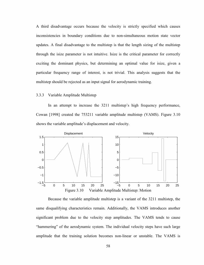
58
A third disadvantage occurs because the velocity is strictly specified which causes
inconsistencies in boundary conditions due to non-simultaneous motion state vector
updates. A final disadvantage to the multistep is that the length sizing of the multistep
through the isize parameter is not intuitive. Isize is the critical parameter for correctly
exciting the dominant physics, but determining an optimal value for isize, given a
particular frequency range of interest, is not trivial. This analysis suggests that the
multistep should be rejected as an input signal for aerodynamic training.
3.3.3 Variable Amplitude Multistep
In an attempt to increase the 3211 multistep’s high frequency performance,
Cowan [1998] created the 753211 variable amplitude multistep (VAMS). Figure 3.10
shows the variable amplitude’s displacement and velocity.
−5 0 5 10 15 20 25−15
−10
−5
0
5
10
15Velocity
−5 0 5 10 15 20 25−1.5
−1
−0.5
0
0.5
1
1.5Displacement
Figure 3.10 Variable Amplitude Multistep: Motion
Because the variable amplitude multistep is a variant of the 3211 multistep, the
same disqualifying characteristics remain. Additionally, the VAMS introduces another
significant problem due to the velocity step amplitudes. The VAMS tends to cause
“hammering” of the aerodynamic system. The individual velocity steps have such large
amplitude that the training solution becomes non-linear or unstable. The VAMS is

59
particularly susceptible to this problem because the velocity ratio of the “7 unit” step to
the “1 unit” steps is 14 to 1. The VAMS is rejected as an aerodynamic training signal.
3.3.4 Chirp
The chirp input signal belongs to the analytic class of input signals. After determining
that the multistep signals have poor motion and frequency excitation properties, a new
class of signals based on frequency sweeps was developed. These signals allow for
smooth transitions in a specific frequency range. Sweep rate and length pairs will be
constrained by Nyquist frequency and data generation requirements. Frequency sweep
parameter selection is discussed further in Appendix C.
The chirp form is based on a linear frequency sweep. Expressions for
displacement, velocity and acceleration are given below. The chirp is analytic
everywhere. The chirp form is:
( )( )
( ) ( )22
2
2
tωttωtatωttv
tωtd
sin4cos2)(cos2)(
sin)(
22ωωω
−==
=
A time history plot of the chirp’s motion for displacement, velocity and acceleration is
given in Figure 3.11. Velocity is scaled by ω-1 and acceleration by ω-2. Velocity envelope
magnitudes increase linearly with time; acceleration magnitudes increase with the square
of time.

60
0 0.1 0.2 0.3 0.4 0.5 0.6 0.7 0.8 0.9 1−1
−0.5
0
0.5
1
0 0.1 0.2 0.3 0.4 0.5 0.6 0.7 0.8 0.9 1−2
−1
0
1
2
0 0.1 0.2 0.3 0.4 0.5 0.6 0.7 0.8 0.9 1−4
−2
0
2
4
Displacement
Velocity/ω
Acceleration/ω2
d(t)=sin(ω t2)
v(t)=2 ω t cos(ω t2)
a(t)=2 ω cos(ω t2) −4ω2 t2 sin(ω t2)
Figure 3.11 Chirp: Motion
A PSD for the chirp is given in Figure 3.12. The chirp sweep length determines
the maximum excitation frequency. This particular signal in Figure 3.12 excites up to
20% of the Nyquist frequency. Because the displacement has constant magnitude, the
PSD is relatively flat for displacement and is sloped at 20 dB per decade for velocity.

61
0 10 20 30 40 50 60 70 80 90 10010
−4
10−2
100
102
Displacement
PS
D
0 10 20 30 40 50 60 70 80 90 10010
−2
100
102
104
Frequency (%Nyquist)
Velocity
PS
D
Figure 3.12 Chirp: Power Spectral Density
The chirp has the following advantages. First, the chirp is an analytic function.
This means that the chirp is consistent with the objective function and is capable of
exciting all aerodynamic motion terms. The chirp starts from zero motion due to zero
frequency at time zero. The chirp’s displacement PSD is approximately flat up to the
excitation sweep length. A final and significant advantage is that the chirp has an
intuitive frequency excitation description. The excitation occurs up to the excitation
sweep length, which is easily determined and specified.
The disadvantages of the chirp are concentrated into two areas. First, the low
frequency performance of the chirp is poor for displacement and even worse for velocity.
The worst PSD for the chirp’s velocity occurs at low frequencies. However, this area is
important for aerodynamic predictions. From the Theodorsen function, the largest phase
difference for unsteady aerodynamics occurs at low reduced frequencies. The second

62
disadvantage results from the analytic nature of the chirp. Since the chirp is analytic, the
system model only contains analytic motion information. Non-analytic motions may not
be accurately represented. The analytic motion differs slightly from the actual system. In
actuality, this difference is significantly smaller than with the pure numerical technique
used for the multistep. This topic will be discussed further in section 3.3.12.
3.3.5 DC-Chirp
To alleviate the low frequency problems inherent in the chirp, a new dc offset
chirp was developed. The result is a non-symmetrical signal with a similar form but with
improved performance when compared to the chirp excitation signal.
The dc-chirp’s form is based on the original chirp. The signal is a linear frequency
sweep from zero frequency. Careful inspection shows that the dc-chirp is a peculiarly
integrated original chirp. Like the original chirp, the signal is analytic everywhere. The
functional form is:
( )( )
( ) ( )22
2
2
tωttωtatωttv
tωtd
cos4sin)(sin)(
cos)(
22
21
21
ωωω
−==
+−=
Figure 3.13 shows the motion history for displacement, velocity and acceleration. The
displacement envelope is held constant. This results in a linear envelope increase for
velocity and a squared increase for acceleration.

63
0 0.1 0.2 0.3 0.4 0.5 0.6 0.7 0.8 0.9 10
0.5
1
0 0.1 0.2 0.3 0.4 0.5 0.6 0.7 0.8 0.9 1−1
−0.5
0
0.5
1
0 0.1 0.2 0.3 0.4 0.5 0.6 0.7 0.8 0.9 1−2
−1
0
1
2
Displacement
Velocity/ω
Acceleration/ω2
d(t)= −2−1⋅ cos(ω t2)+2−1
v(t)= ω t sin(ω t2)
a(t)= ω sin(ω t2) + 2ω2 t2 cos(ω t2)
Figure 3.13 DC-Chirp: Motion
A PSD for the dc-chirp is given in Figure 3.14. Again, the frequency is swept to
20% of the Nyquist frequency. Careful inspection shows that the low frequency power
for the dc-chirp is increased over the original chirp’s power. The velocity PSD has the
same undesirable form as the original chirp at low frequencies.

64
0 10 20 30 40 50 60 70 80 90 10010
−10
10−5
100
105
Displacement
0 10 20 30 40 50 60 70 80 90 10010
−2
100
102
104
106
Frequency (%Nyquist)
Velocity
Figure 3.14 DC-Chirp: PSD
The dc-chirp has the same advantages as the original chirp plus additional low
frequency displacement power due to the dc offset. The dc-chirp allows for a visual
determination of rate and displacement effects because the displacement motion is offset
and the velocity is symmetrical. The different motion forms allow for improved
distinction between the effects of displacement and velocity. Figure 3.15 shows a classic
example of this motion distinction.

65
0 50 100 150 200 250 300 3500
0.2
0.4
0.6
0.8Displacement
0 50 100 150 200 250 300 350−0.05
0
0.05Velocity
0 50 100 150 200 250 300 350−40
−20
0
20Forces
Zero
Figure 3.15 DC-Chirp: Motion Determination Example
The dc-chirp has many of the same disadvantages as the original chirp. Adding
the dc offset removed the PSD problem at low frequencies for the displacement;
however, little power is being applied to the velocity at low frequencies. A subtle second
disadvantage concerns the peak factor of the dc-chirp compared to the original chirp.
Because the new dc-chirp is non-symmetrical, the absolute forced magnitude of
displacement is only half that of the original chirp with a maximum displacement of
unity. Doubling the dc-chirp’s magnitude to achieve a similar power level pushes the dc-
chirp closer to the non-linear aerodynamics regime.
3.3.6 Fresnel Chirp
The Fresnel chirp is a linear frequency sweep with a displacement as the true
integral of the original chirp. The Fresnel chirp is expected to increase the low frequency
velocity power. The result is an excitation signal with no closed form expression but with
potential for better training performance.

66
The Fresnel chirp is an integrated form of the original chirp. The Fresnel chirp
still contains a linear frequency sweep and is analytic everywhere. As a practical
implementation issue, there are two forms of the Fresnel chirp. The two forms result from
the integration of either the sine or cosine function. The signal needs to start from rest, so
the Fresnel sine function, S(t), is chosen. The functional form is:
( )( )
( )2
2
2
tωttatωtv
tωtStd
cos2)(sin)(
sin)()(
ω==
== ∫
A motion history for the Fresnel chirp is given in Figure 3.16. An envelope
magnitude occurs for the Fresnel chirp’s velocity. As expected by integration theory, the
displacement tapers down in magnitude as frequency increases. A PSD for the Fresnel
chirp is given in Figure 3.17.
0 0.1 0.2 0.3 0.4 0.5 0.6 0.7 0.8 0.9 1
−1
−0.5
0
0.5
1
0 0.1 0.2 0.3 0.4 0.5 0.6 0.7 0.8 0.9 10
0.2
0.4
0.6
0.8
Displacement
Velocity
d(t)=S(t)= ∫ sin(ω t2)
v(t)=sin(ω t2)
Figure 3.16 Fresnel Chirp: Motion

67
0 10 20 30 40 50 60 70 80 90 10010
−4
10−2
100
102
104
Displacement
PS
D
0 10 20 30 40 50 60 70 80 90 10010
−4
10−2
100
102
Frequency (%Nyquist)
Velocity
PS
D
Figure 3.17 Fresnel Chirp: PSD
The Fresnel chirp has significant advantages over those of the previous chirps.
The largest improvement consists of the “flat” velocity PSD. Velocity power is still weak
for low frequencies, but an integrated dc-chirp cannot be implemented because
integrating an offset signal yields a diverging signal. Integrating a non-symmetrical
velocity signal will cause displacement peak factor problems. A minor disadvantage of
the Fresnel chirp is that the resulting function has no simple, closed form solution and
requires numerical integration for practical implementation [Zwillinger, 1996]. The noisy
displacement PSD appears to be a result of the integration scheme introducing noise into
the displacement signal. Noisy integration may become a sensitivity issue later.

68
3.3.7 Schroeder Sweep
The Schroeder excitation signal is based on the multisine class of signals. This
class of signals allows for the specific excitation of a specified bandwidth through the
summation of discrete frequencies. A phase-shift presented by Schroeder [1977] allows
for minimizing the signal’s peak factor.
The Schroeder form is based on a sum of cosine terms with a specified phasing.
Expressions for displacement and velocity are given below. The form is analytic in time
but not smooth in frequency.
∑
∑
=
=
−−=
−=
N
k
N
k
Nk
Ttk
NTktv
Nk
Ttk
Ntd
1
2
1
2
2sin212)(
2cos21)(
πππ
ππ
Figure 3.18 plots the displacement and velocity for a 50-term Schroeder sweep.
The signal is harmonic and can continue indefinitely. The signal resembles a frequency
sweep during a significant portion of the time history. The Schroeder sweep appears to be
the discrete time counterpart to the continuous-time frequency-swept chirps. The
displacement is bounded by a unit magnitude envelope.

69
0 5 10 15−1
−0.5
0
0.5
1Displacement
0 5 10 15−30
−20
−10
0
10
20
30Velocity
Figure 3.18 Schroeder Sweep: Motion
A PSD for the Schroeder sweep is given in Figure 3.19. The number of terms in
the summation determines the sweep bandwidth. The PSD is flat along the excitation
bandwidth. This particular signal excites up to 20% of the Nyquist frequency. Careful
inspection shows that a pure dc component exists. The sweep is implemented on
displacement, so the velocity PSD exhibits the expected sloped response. However, the
Schroeder sweep could be implemented on velocity with only minor changes.
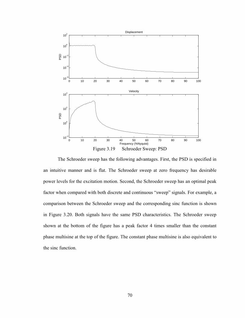
70
0 10 20 30 40 50 60 70 80 90 10010
−6
10−4
10−2
100
102
Displacement
PS
D
0 10 20 30 40 50 60 70 80 90 10010
−2
100
102
104
Frequency (%Nyquist)
Velocity
PS
D
Figure 3.19 Schroeder Sweep: PSD
The Schroeder sweep has the following advantages. First, the PSD is specified in
an intuitive manner and is flat. The Schroeder sweep at zero frequency has desirable
power levels for the excitation motion. Second, the Schroeder sweep has an optimal peak
factor when compared with both discrete and continuous “sweep” signals. For example, a
comparison between the Schroeder sweep and the corresponding sinc function is shown
in Figure 3.20. Both signals have the same PSD characteristics. The Schroeder sweep
shown at the bottom of the figure has a peak factor 4 times smaller than the constant
phase multisine at the top of the figure. The constant phase multisine is also equivalent to
the sinc function.

71
-1
0
1
0
1
2
3
4
N
kk
2
1
πθθ −=
∑=
+=
N
k
kk
T
tkptr
1
2cos
2)( θ
π
2
πθ =k
Phasing:
Basis Function with N=30
Npk /1= (equal power at all frequencies)
Figure 3.20 Schroeder Sweep: Peak Factor Comparison
The disadvantages are concentrated in three areas. First, the Schroeder sweep
does not intrinsically contain a from-rest starting condition. Any attempt at using the
Schroeder sweep requires a modification to establish both the steady state system
behavior and the from-rest starting response. Bounding the sweep with an envelope will
cause undesirable and non-intuitive distortions of the signal’s characteristics. Simon
[2000] shows the undesirable results of harmonic signal truncation. Testing with the
Schroeder sweep verified this sensitivity. Second, the Schroeder sweep requires a
numerical sum of terms at each timestep. This summation is expensive for large
excitation bandwidths. The third disadvantage is that the Schroeder sweep, being a
harmonic signal, appears to be excessively sensitive to excitation length. Testing shows
that small errors in signal specification can cause regular holes in the Schroeder’s PSD.
These types of sensitivities are not desired for robust training.

72
3.3.8 Noise Training Signal
A final class of signals is based on stochastic system theory. White noise is
defined as a signal with equal power at all frequencies. A white noise input signal would
allow for equal excitation up to the Nyquist frequency. A white noise signal with 500
data points is given in Figure 3.21.
0 0.1 0.2 0.3 0.4 0.5 0.6 0.7 0.8 0.9 1−1
−0.5
0
0.5
1
Figure 3.21 Noise: Displacement
A PSD for white noise is given in Figure 3.22. This plot uses 500 samples. A
second PSD for white noise with 5000 samples is given in Figure 3.23. Excitation length
strongly determines the PSD distribution characteristics. A constant PSD over the entire
frequency range requires an infinite excitation length.
0 10 20 30 40 50 60 70 80 90 10010
−3
10−2
10−1
100
101
PS
D
Figure 3.22 Noise: PSD 500 Samples

73
10−6
10−4
10−2
100
102
PS
D
Figure 3.23 Noise: PSD 5000 Samples
The white noise input signal has advantages. First, the PSD is defined to be “flat”.
The signal can start from rest and has no restrictions on excitation length. Unlike the
analytic signals, the white noise input will excite the non-harmonic components in the
aerodynamic system.
There are numerous disadvantages to the white noise signal. First, the “flat”
power level is only achievable as the excitation length becomes infinite. Therefore, the
excitation length is non-intuitive. The implementation question becomes: How long is
long enough? A related disadvantage is that the training signal is not deterministic. The
signal is unknown random noise. Traditional statistical data allows for comparisons
between the noise properties but does not allow for input-output comparisons. The noise
input signal is not guaranteed to excite the same system dynamics between two otherwise
identical simulations. Comparison of non-deterministic training signals is likely to
encounter difficulties. Second, the noise input signal creates problems with boundary
conditions in two ways. The first is that the input excitation is not consistent with the
discrete-time solution method. Equal power at the frequencies near Nyquist implies that
“sharp” changes occur in the input signal. These changes will overdrive the flow solution
solver. The motion time history in Figure 3.21 shows this characteristic of the signal. An
example of this problem would be an excitation that moves an airfoil so quickly that the

74
flow solution becomes dominated by shock acoustics, which violate the linearity
assumption. The second boundary condition problem is that simultaneous updating of
motion states is not possible. Because the signal is not deterministic, generating
displacement from velocity, or vice versa, requires numerical integration. Numerical
integration introduces time lags and is not consistent with the ARMA motion
specification. These disadvantages require that the noise signal be rejected as an input
signal.
3.3.9 Envelopes
A complication arises with some signals because their harmonic form does not
allow initial starting conditions without impulsive transients. A general method of either
beginning or ending the excitation when the excitation does not begin at zero is needed.
One solution is to develop an envelope term that starts or stops the input signal from a
zero motion condition.
Combining two exponential functions allows for a generic envelope function. An
envelope function based on this concept is given below. The power constant of 11 is
empirically determined based on function roll-off requirements. Higher power constants
yield sharper roll-offs. The envelope form is:
110
110 )exp()exp()( tttttenv −⋅−−=
While the above form appears only useful for ending conditions, the following
transformation allows for specifying a zero motion starting condition:
)(1)( tenvtenvstart −=
The above forms are poorly suited for numerical evaluation. A better numerical
expression is found by expanding into the following form:

75
( )100
830
650
470
290
110 223309246601102exp)( ttttttttttttenv ⋅−⋅−⋅−⋅−⋅−⋅−=
The effective time of roll-off is determined through the t0 term. Practically, this term
must be determined empirically; a general solution is not intuitive. However, a more
powerful technique is to non-dimensionalize the envelope time terms and then re-
dimensionalize the envelope for the particular timescale. Setting t0 equal to 1.0-10
specifies an envelope with a magnitude of approximately 0.1% of the initial value at a
non-dimensional time of unity. Figure 3.24 shows the time form of the envelope.
0 0.1 0.2 0.3 0.4 0.5 0.6 0.7 0.8 0.9 10
0.2
0.4
0.6
0.8
1
Non−Dimensional Time
Envelope Magnitude
Figure 3.24 Envelope Form
3.3.10 Superposition of Multiple Signals
The objective is to supplement the regular training signal by adding extra signals
through superposition. Adding signals together allows for the possibility of exciting
multiple frequency ranges without using a single long sweep. However, this type of
superposition assures phase and frequency interference because the training signals have
restrictions on the starting conditions. As a result, the power spectral density has sharp
holes at the interference frequencies. Figure 3.25 shows the PSD of a superposition of a
chirp signal, a low frequency chirp signal and the resulting summed signal. The peak
factor is held constant.

76
102
10 1
100
10 1
100
101
102
Chirp Signal
Low FrequencyChirp
Sum
PSD
Frequency Figure 3.25 Superposition of Multiple Signals: PSD Holes
Sharper holes are created in the summed signal. This example shows the importance of
both magnitude and phase in signal superposition. These PSD characteristics of summed
signals show the difficulties of signal design with respect to peak factors. Choosing a
globally optimal signal appears to be better than choosing and combining several locally
optimal signals.
3.3.11 Purposefully Added Noise
Contrary to intuition, adding noise to an existing signal is often desired for system
identification. This occurs because many signals, like the chirp, only excite a specific and
limited frequency spectrum due to simulation time and aerodynamic convergence
concerns. This causes problems when the system identification correlates small
perturbations in the input signal with numerical artifacts in the output signal. The
resulting relationship between input and output becomes dominated by numerical
artifacts rather than the underlying physical system. Viewing the problem from a transfer
function approach yields the same conclusion. A ratio of output to input is not specified

77
by the absolute magnitudes of input and output. This situation occurs regardless of the
identification method used; it is the result of the training method. Specifically, the
numerical convergence of a frequency power level must be consistent between the input
and output. For strictly defined functions, the input noise is on the order of the storage
numerical accuracy. This problem typically occurs at high frequencies where the training
signals have little or no power. The problem surfaces as spurious and non-physical
eigenvalues in the complex z plane.
One solution is to add artificial noise to cover the high frequency spectrum. White
noise offers a wide frequency excitation when given sufficient excitation length. The
noise only needs to increase the input signal power levels; a corresponding increase in the
output is not necessary. To visually display this concept, a noise comparison experiment
was developed. The experiment used a subsonic two-dimensional airfoil with a single
pitch mode to generate the output signal. The input signal to the CFD solver was the
clean signal shown the lower plot of Figure 3.26. A noisy input signal was generated by
superimposing the clean signal with low amplitude white noise. The upper plot of Figure
3.26 shows this noisy signal. The same clean output signal was used for both the noisy
and clean systems. Thus, both systems use the same output with different inputs. The
noise was added to the input signal after the CFD solver but before the system
identification. This is only a conceptual experiment; an actual identification would not
use this ad-hoc noise augmentation method. The objective is to show the effect of signal
spectral content without introducing CFD related uncertainties and complications.

78
0 0.5 1 1.5 2 2.5 3 3.5
0
5
10
Noisy
1
0 0.5 1 1.5 2 2.5 3 3.5
0
5
10
1
Clean
Figure 3.26 Noise Experiment: Noisy and Clean Input Signal
A transfer function comparison is made from the raw input and output signals. To
achieve a fair comparison of the clean and noisy systems without generating intermediate
system models, the transfer functions were generated as the ratio of power-spectral-
densities of the output over the input. Figure 3.27 plots the frequency dependent transfer
function for the clean signal. Figure 3.28 plots the transfer function for the noisy signal.
For the clean signal, the transfer function form appears smooth; however, the
form does not agree with either intuition or physics. Regardless of what the system
transfer function indicates, forcing the system at the Nyquist frequency should not result
in a factor of 1020 more output than the steady state response. Output power converges to
a PSD level of approximately 10-13 at high frequencies due to the CFD solution
limitations. Yet, the input signal continues to decrease in power level as frequency
increases because the input signal is strictly defined as a mathematical function. Forcing
more noise in the input signal will assist finding a better system transfer function.
For the noisy signal, the transfer function does not appear smooth because the
white noise excitation is limited in length. However, the ratios of input and output powers
appear more consistent. The transfer function captures the dominant low frequency
structure of the aerodynamics without an overwhelming response at high frequencies.

79
0 10 20 30 40 50 60 70 80 90 10010
30
10 25
10 20
10 15
10 10
10 5
100
105
1010
1015
Transfer Function
Output
Input
Frequency (% Nyquist)
Power Spectral Density
Figure 3.27 Noise Experiment: Transfer Function with a Clean Input Signal
0 10 20 30 40 50 60 70 80 90 10010
14
10 12
10 10
10 8
10 6
10 4
10 2
100
Power Spectral Density
Transfer Function
Output
Input
Frequency (% Nyquist)
Figure 3.28 Noise Experiment: Transfer Function with a Noisy Input Signal
A second comparison is made with the coupled aerostructural system’s
eigenvalues. For this comparison, the low frequency eigenvalues inside the input training
signal’s main excitation sweep are ignored. The eigenvalues under consideration are
those higher than approximately 10 percent of the Nyquist frequency. Figure 3.29 plots
the eigenvalues in the z plane for the clean input signal. Undesirable eigenvalues at high
frequencies emanate from the origin as dynamic pressure is increased. These correspond
to the large magnitudes of the transfer function at high frequencies. Eigenvalues for the
noisy input signal are plotted in Figure 3.30. In contrast to the clean signal, the high
frequency eigenvalues for the noisy signal remain near the origin.

80
−1 −0.5 0 0.5 1−1
−0.8
−0.6
−0.4
−0.2
0
0.2
0.4
0.6
0.8
1
Real(z)
Imag
(z)
Figure 3.29 Noise Experiment: Eigenvalues with Clean Input Signal
−1 −0.5 0 0.5 1−1
−0.8
−0.6
−0.4
−0.2
0
0.2
0.4
0.6
0.8
1
Real(z)
Imag
(z)
Figure 3.30 Noise Experiment: Eigenvalues with Noisy Input Signal
Conceptually, the addition of high frequency power to the input training signal
improved the system identification model’s accuracy and performance. For high fidelity
simulations such as controls, the clean signal would cause significant simulation
problems, while the noisy signal would allow simulations that are more precise,
especially at high frequencies. It appears that storing and changing the input and output
vectors should be numerically consistent.
3.3.12 Motion Specification
This section investigates input signal motion specification. Two choices exist for
specifying the input training motion: strict motion specification and state-space motion
specification.
It is important to understand why motion specification is important. The ARMA
model associates forces with past and previous displacements and past forces. Only
through consistent boundary conditions is the ARMA form able to “see” velocities and
higher derivatives. The result is that the system identification routine requires a training

81
method consistent with the boundary conditions and the motion state update
methodology.
3.3.12.1 Strict Motion Specification
Strict motion specification is the current methodology. For strict motion
specification, the motion state vector at each timestep is determined from either an
analytical or a numerical expression without reference to the previous motion state
variable. For analytical input signals, this method results in “perfect” signals with
perfectly correct integrals and derivatives. For example, the dc-chirp and its derivative
could be used to directly determine the boundary conditions at any timestep.
The advantage of strict motion specification is that the implementation is simple.
The method only requires directly setting the boundary conditions inside the CFD solver.
The CFD flow solver does not care if the boundary conditions make no sense; the flow
solver will still output a solution.
The disadvantage of strict motion specification is important. Strictly specifying
the boundary conditions requires consistence in the discrete time sense. The method
requires either a continuous time derivation or a discrete time numerical operation.
Neither is correct.
3.3.12.2 State Space Motion Specification
An alternative method for motion specification is through a state space update
methodology. The boundary conditions are updated through a state space form with the
excitation signal not directly specifying the state vector. This is a methodology identical
with structural excitation with an external force function. Implementing this methodology

82
involves the derivation given in section 2.6.3. This methodology resembles the excitation
of a mechanical system without stiffness or damping.
The advantages of this methodology are significant. The boundary conditions are
updated simultaneously in a true discrete time sense. The excitation signal and response
is consistent with the coupled aero-structural response. Additionally, non-analytic input
signals are no longer a problem because the input is filtered through the “structure”. A
convenient advantage of this methodology is that the state space update routines already
exist in the CFD solver; there is no code development required.
The disadvantages of this motion specification methodology are slight. The
methodology requires selecting a force versus “structural mass” ratio that excites the
system within the linear limitations. Maximum magnitudes are not directly specifiable as
in the strict motion methodology. The biggest disadvantage is the stopping condition.
Because the excitation signal is input on acceleration, ending the excitation does not
result in the motion returning to zero. Instead, the mode will continue to move with
constant velocity after the excitation is removed. This can result in motions that exceed
linearity limitations. This requires an ending condition specification that requires the
velocity and displacement to remain within certain bounds. Practically, this can be
handled with a crude force feedback loop on displacement.
3.4 Model Performance Evaluation Criteria
This section seeks effective methods of comparing and selecting ARMA models
based on model performance. The fundamental difficulty is that all reasonable models fit
the training signal, so comparison and selection by visual inspection of time histories is
doomed to failure. However, any model not fitting the training signal is automatically

83
rejected. The preferred selection technique is to use a numerical measurement. Also, any
information on actual system model order is desired.
3.4.1 Chi Squared
Chi-squared error, 2χ , gives an indication of how well the SVD model fits the
training data. This is an indication of solution quality, not model performance quality.
The characteristics of the chi-squared error resemble the model fit least square error. Chi-
squared error is calculated with the following expression:
nstpbxA 2
2 −=
r
χ
The overall fit-error is divided by the number of time steps in the training signal, which
ensures a fair comparison between variable length signals. Otherwise, 2χ always
increases with an increase in data points for the same model.
Chi-squared error converges to zero as the number of model coefficients
approaches infinity. This is expected because more coefficients allow a closer fit
regardless of the resulting model quality. A typical plot of 2χ error and model order is
shown in Figure 3.31.

84
0 20 40 60 80 100 120 140 160 180 20010
−6
10−4
10−2
100
102
Number of Model Coefficients
χ2
Figure 3.31 Chi Square: Typical Two Mode Plot
The advantage of using chi-squared error as a selection criterion is that chi-
squared error directly relates to the solution quality. Large chi-squared errors indicate
poor model performance, which is caused by the model not accurately fitting the training
data. Global chi-squared magnitudes indicate the amount of noise contained in the
training signal. Another advantage is that determining chi-squared error is
computationally cheap; only one matrix multiplication is required.
The primary disadvantage of chi-squared error is that it is not useful for model
performance characterization. Since the chi-squared error always decreases for increasing
model order, it does not allow for model order estimation. Low chi-squared error is a
necessary, but not sufficient, condition for good quality aerodynamic models.
3.4.2 Force Prediction Root Mean Square
The force prediction RMS gives a measure of forced response prediction with a
known signal. Typically, the force RMS is applied to the training signal; however, any
signal is applicable. The force RMS calculation is made with the following expression
where )(ky refers to the predicted force vector and )(ˆ ky refers to the actual force vector:

85
( )∑=
−=N
kkyky
NRMS
0
2)(ˆ)(1
The force RMS provides significantly better model performance information than chi-
squared error because the force RMS system model contains aerodynamics indexed to the
starting conditions which are not reset to the known signal at each timestep. Unlike chi-
squared error, force RMS evaluates the true system performance for a connected time
history.
An example force RMS plot versus model coefficients for a two mode testcase is
given in Figure 3.32. For this testcase, the force RMS converges to near a minimum value
and then varies around a mean point. With further increases in model order, the RMS
slowly increases.
0 20 40 60 80 100 12010
−3
10−2
10−1
Number of Model Coefficients
Force RMS
Figure 3.32 Force RMS: Two Mode Testcase
While the force RMS does not appear to be an effective model order determination
criterion, it does give an indication of model quality.
3.4.3 Partial Autocorrelation
The partial autocorrelation correlates the response dependencies at each time with
all other times. Conceptually, PACF information could determine a limiting model order

86
that captures the dominant dynamics. The model order could be sized based on where the
PACF becomes effectively zero. This could potentially eliminate the current brute force
model selection methods. However, Brockwell [1991] points out a significant limitation
of the PACF:
In contrast with the partial autocorrelation function of an AR(p) process,
that of an MA(q) process does not vanish for large lags. It is however
bounded in absolute value by a geometrically decreasing function.
This indicates that the PACF would not provide accurate model order data for ARMA
models. For comparison, Figure 3.33 plots the PACF for an actual subsonic aerodynamic
system generated with CFD and a chirp training signal.
Figure 3.33 PACF: Aerodynamic System with Chirp Training Signal
The response curve of Figure 3.33 appears to agree with Brockwell’s prediction. No clear
minimum-model-order lag time stands out.
3.4.4 Coupled Aero-Structural Properties
A powerful model performance criterion is based on the coupled aero-structural
properties exhibited by the model. Using the model for coupled aero-structural
predictions exercises the model’s prediction characteristics in a realistic and intuitive

87
manner. This criterion allows for both individual and multiple model performance
evaluations.
This criterion is based on eigenvalue predictions. The eigenvalues are calculated
from a coupled aero-structural state transition matrix. Calculating eigenvalues
corresponding to the aerodynamic state-space model will only show the internal system
response and not the input-output response. This would be a major limitation for model
performance evaluation. The simple solution is to include structural dynamics. Using the
coupled aero-structural derivations given in section 2.6.3, a discrete time plant matrix is
determined. The expression is reproduced below:
+ ∞∞
asa
assass
GCHCHqCDHqG
Dynamic pressure, q∞, is an independent variable. Plotting the eigenvalues in the discrete-
time z plane over a range of dynamic pressures yields both stability boundary and model
sensitivity information. A typical root locus plot for a density sweep from 0 to 20 units of
dynamic pressure is given in Figure 3.34.
Figure 3.34 Eigenvalue Explanations

88
Because the plant matrix contains both the structural and aerodynamic systems,
eigenvalues corresponding to both systems appear. Structural motion eigenvalues begin
at the free vibration frequency for zero dynamic pressure. Eigenvalues corresponding to
the ARMA model are seen as the set of curves emanating from the z plane’s origin. The
model’s sensitivity to dynamic pressure and suitability to controls applications can be
determined from the eigenvalue locations and motion.
Evaluating multiple models allows for model order sensitivity studies. A typical
model order sensitivity plot is given in Figure 3.35.
0 10 20 30 40 50 60100
110
120
130
140
150
160
0
1
2
nb Order
Dyn
amic
Pre
ssur
e na Order
Figure 3.35 Model Order Sensitivity Explanation
For this plot, dynamic pressure for neutral stability is plotted for a range of na and
nb model orders. It is desired that the dynamic pressure for neutral stability converge
with both na and nb terms. Figure 3.35 is an example of poor convergence. Figure 3.36
shows excellent convergence.

89
0 5 10 15 20 25 300.4
0.45
0.5
0.55
0.6
0.65
0.7
0.75
0.8
1 23456789101112131415161718192
nb Order
Dyn
amic
Pre
ssur
e
na Order
Figure 3.36 Model Order Sensitivity Convergence
A second type of eigenvalue sensitivity study is to plot the coupled aero-structural
eigenvalues for a range of dynamic pressures over a range of model orders. This study
indicates the degree of model prediction consistency. Typically, the eigenvalues of
concern for this type of study are those corresponding to the structural motion. Figure
3.37 shows a typical model sensitivity study with the coupled eigenvalues in the z plane.
The figure is zoomed to show only the structural eigenvalues. This particular testcase has
six modes.
Figure 3.37 Eigenvalue Sensitivity Study Explaination

90
For this example, the eigenvalues converged as the model order was increased
from 2-8 to 6-16. An order of 10-20 yields a slightly different eigenvalue structure. A
model order of 6-16 seems to be the best. This type of sensitivity study provides a
powerful method to evaluate the resulting aerodynamic system models.
The advantages of using coupled aero-structural performance evaluation criteria
are significant. First, coupling the two systems allows for evaluating a more complex
combined system. This combined system reveals problems more readily and tests the
system model in a realistic environment. This method allows for system property
evaluations that would be utterly invisible when comparing the responses in the time
domain.
There are disadvantages to using a coupled system performance criteria. The
method requires significant computational effort. Because the aerodynamic model order
changes, individual eigenvalue sweep comparisons for the aerodynamic terms are not
possible in the z plane.
3.5 Preliminary Testcases
These examples consist of simple testcases with known solutions. The objective is
to investigate system identification performance on simple testcases. This should assist
will interpretating and evaluating more complicated actual testcases.
3.5.1 Zero Order Force Function
This testcase consists of a forcing function that only depends on the current
motion. This results in a zero order differential equation: xqf &= . The resulting force is
coupled with a single degree of freedom structural system. The representation of the

91
overall structural system is fxkxcxm =++ &&& . From the simple force model, xqf &= , a
simple chirp training signal was used to generate an input motion versus output force
relationship.
Figure 3.38 Zero Order Force Training Signal and Output
From this training signal, three ARMA models were generated. Because the
current ARMA model structure stores only the displacements, the resulting ARMA
model should return the coefficients for a first order derivative. The model should contain
coefficients for a first derivative of equally spaced points with the derivative taken at the
endpoint. The following table shows the resulting non-dimensional ARMA model
coefficients and the exact coefficients from a Taylor series expansion. The ARMA
coefficients are non-dimensionalized by )!1(1 −ph , where p is the number of points and
h is the point spacing.

92
2 Pt 3 Pt 4 Pt
Step Taylor Series ARMA
Taylor Series ARMA
Taylor Series ARMA
n 1 1.007 3 2.9990 11 9.078 n-1 -1 -1.018 -4 -3.9981 -18 -12.235 n-2 1 0.9989 9 3.239 n-3 2 -0.082
χ2 0.39·10-2 0.29·10-5 0.28·10-5
Table 3.1 1st Derivative Comparison for Taylor series and ARMA coefficients
The coefficients from theory and ARMA agree for the 2 and 3 point derivative
expressions. The 4 point expression does not match other than qualitatively. However,
the 4 point derivative offers no better fit than the 3 point. This suggests that the model has
converged and extra data points are not likely to improve the data fit. The output fit
parameters χ2, RMS and autocorrelation (ACF) are plotted in Figure 3.39 for nb model
orders from 2 to 6. RMS and chi-squared errors level off at three terms. It appears that the
first bump of ACF corresponds to leveled RMS and chi-squared error.
Figure 3.39 Output Fit Parameters
Next, the entire system’s stability is investigated. The governing differential
equation is xqxkxcxm &&&& =++ . The system is expected to become unstable at cq >

93
when damping becomes zero. In state space form with the structural damping in terms of
the forcing function, the overall structural system becomes the following:
−−−=
xx
mqc
mk
xx
&&&
& 10
The system was discretized with the parameters given in Table 3.2:
Mass m 1.0Stiffness k 4.0Damping c 0.1Time Step ∆T 0.1
Table 3.2 0th Order Forcing Function Structural Parameters
The discrete time state space model becomes:
=
++
)()(
)1()1(
kxkx
Akxkx
d &&
The state transition matrix, Ad, is the following expression, which is in terms of structural
and aerodynamic parameters:
( )( )( )( )
−−⋅⋅−−
−⋅+⋅⋅=
xCqcSzzSzSqcSxCz
Ayyy
yyyd 2
2
The coefficients used above are factored using the following coefficients:
( )( )
)sin()cos(
)(exp
24
121
21
22
ySyC
qxtqcz
txyqcqckx
y
y
=
=⋅∆⋅−−=
∆⋅=−+−=
−
At zero dynamic pressure, q=0, the state transition matrix is the following:
−
=97.0395.0099.098.0
dA

94
Plotting the eigenvalues of this system over a range of dynamic pressures of 0 to 20
yields Figure 3.40 and the zoomed eigenvalue crossing Figure 3.41. The eigenvalues
cross the unit circle at a dynamic pressure of 0.1 as expected. At a dynamic pressure of
4.1, the eigenvalues meet at the real axis and the structure becomes statically divergent.
Figure 3.40 Zero Order Forces: Eigenvalues
Figure 3.41 Zero Order Forces: Zoomed Eigenvalue Crossing
Now, the coupled aero-structural eigenvalues are determined using system identification.
Figure 3.42 plots the eigenvalues for model orders from 0-2 to 0-7. The structural
eigenvalues qualitatively match the exact form shown above. All models determine a
stability boundary at a dynamic pressure of 0.1.

95
0-2 Model
0-3 Model
0-4 Model
0-5 Model
0-6 Model
0-7 Model
Figure 3.42 Zero Order Forces: System Identification Eigenvalues.
The extra aerodynamic states appear as eigenvalues moving away from the origin. The
frequency spacing of these extra terms are constant, which reveals the equally spaced
discrete-time form of the ARMA model.
3.5.2 Second Order Force Function
A more complicated example is created using the same structural system and a
more complicated forcing function. This testcase consists of a forcing function that
depends on a second order ODE. The differential equation for force is:
xxfff &&&& 1.082 +=++
f is an output and x is an input. Converting the system to a state space form with the
states [ ]Tfff &r
= yields the following:
[ ] [ ]xBfAxx
ff
ff rr
&&&&
&+=
+
−−
=
1.01
0028
10

96
For the continuous case, determining an analytical stability boundary is possible
by coupling the structural and forcing systems and evaluating the resulting system.. The
structural parameters are given in Table 3.2. These are the same structural parameters as
used in the previous section. Coupling the aerodynamic and structural systems yields the
following continuous time state space system:
−−
−−
=
∞
xxff
qxxff
&
&
&
&&
&
&&
010041.00
000111.082
Computing the eigenvalues over a range of dynamic pressures yields a divergence
stability boundary at a dynamic pressure of 32. The continuous time root locus plot is
given in Figure 3.43. The eigenvalue at zero frequency and at a positive real value shows
that the system becomes unstable through divergence. Aerodynamic eigenvalues are seen
near 38.0 ±−=s .
Figure 3.43 2nd Order Force: Continuous-Time Root Locus

97
Next, this coupled system was converted to a discrete time system. A step size of 0.1 was
used to generate the following discrete time root locus plot.
Figure 3.44 2nd Order Force: Discrete-Time Root Locus
The dynamic pressure for divergence remains at 32. The system identification routine
should show a similar root locus form.
The above continuous system was converted to a discrete time state space form
with use of the matrix exponential. With a discrete step size of 0.1, the discrete state
space form is:
[ ]( )
⋅−⋅−⋅
=−=
−
=≈=
−
−−−
=
⋅ ∑
3
431
0
10943.8089.010652.410652.4
784.0715.0089.0963.0
!1
BIAAB
Adtk
eA
dd
n
k
kkdtAd
The total discrete time state space form is:
)()()1( kxBkfAkf ddrrr
+=+

98
Next, this discrete system was implemented in a simple spreadsheet. A simple
chirp excitation signal was input as xr into the system and an output force fr
was
recorded. The input displacement and output force is shown in Figure 3.45. The output
increases in amplitude due to the contribution from x& as the input displacement
frequency increases.
Figure 3.45 2nd Order Force: Dynamic Input and Output
For comparison, a model sensitivity study was performed. The model order was
varied from a 0-2 to a 10-20. The forced RMS error is plotted in Figure 3.46.

99
2 4 6 8 10 12 14 16 18 2010
−8
10−6
10−4
10−2
100
102
0
1
2345
678910
nb Order
RM
S na Order
Figure 3.46 2nd Order Force: RMS Error Study
na orders of zero and one never converge. The first model with an RMS error less than
10-4 is the 3-2 model. Increasing the nb model order can allow for a good model even
with small na model orders. The RMS error converges for all nb orders with na greater
than 3. For this simple system, the RMS error allows for model order determination.
A coupled aero-structural sensitivity study was performed. Figure 3.47 plots the
divergence dynamic pressure versus na and nb model order. This testcase uses the chirp
training signal.
2 4 6 8 10 12 14 16 18 200
5
10
15
20
25
30
35
40
0
1
2 3 45678910
nb Order
Dyn
amic
Pre
ssur
e
na Order
Figure 3.47 2nd Order Force: Divergence Boundary Study

100
The boundary converges for model orders greater than na equal to 1. The converged
divergence boundary is located at a dynamic pressure of 32.0. This is exactly the
analytical boundary.
An eigenvalue sensitivity study was performed to evaluate the system
identification root locus with respect to the previous analytical result. Figure 3.48 shows
the discrete time eigenvalues for model order of 3-2, 3-5 and 5-10. The eigenvalues
follow the structure given in the analytical case. The system identification and aeroelastic
coupling procedures appears to be working correctly.
−1 −0.5 0 0.5 1−1
−0.8
−0.6
−0.4
−0.2
0
0.2
0.4
0.6
0.8
1
Real(z)
Imag
(z)
Figure 3.48 2nd Order Force: Root Locus Study
The aerodynamic eigenvalues calculated with system identification appear to “pull”
towards the origin more than the analytical results. The presence of additional
eigenvalues near the unit circle is probably responsible for the difference.
Next, a 20-100 model was evaluated to test the performance of vastly-too-large
models. An eigenvalue plot is shown in Figure 3.49. The important aerodynamic and

101
structural eigenvalues match those of the lower order models and the analytical result.
The spurious eigenvalues that approach the unit circle are discussed in 3.3.11 and 3.3.12.
Figure 3.49 2nd Order Force: Root Locus Study with a Large Model
System identification found the dominant aerodynamics and accurately predicted the
divergence boundary for this simple testcase.

102
CHAPTER 4
4RESULTS
This chapter presents results from aeroservoelastic testcases with the experience
gained from the methodology section.
4.1 Aerodynamic System Identification Training Method
This section briefly outlines the system identification training method.
• Steady State: Run steady euler3d to obtain a steady .unk solution file
• Modeshapes: Run Solids to obtain structural modes. Convert the solids
modeshapes to euler3d .vec file format.
• Convergence: An accurate unsteady solution requires convergence.
Ensure convergence of the unsteady solution with the proper selection of timestep
and iterative parameters in euler3d. Inputting a step response is a good way to test
for unsteady convergence. The following shows the convergence requirements to
ensure solution accuracy. For example, structural motion convergence is ensured
through a sufficient number of structural modes. Adding additional structural
modes is moderately difficult. The “easy” solution convergence requirement
should be checked at every timestep. The CFD grid is difficult to change.
Converged is performed by comparing the solutions to successively refined grids.
All four of these convergence criteria must be satisfied to ensure an accurate
aeroservoelastic solution.

103
Convergence: Difficulty Solution via residuals Easy Time via timestep ... Structure via number of modes ... CFD Grid via grid refinement Hard
• Training Signal Parameters: Select training signal parameters based on
physics and convergence criteria.
• traincreate3d: Create a training directory structure and copies the grid,
modeshape and control files for each mode.
• euler3d: Run unsteady chirp training signal for each mode
• trainassemble3d: Assemble all xn.dat outputs to a single assemble directory.
Rename each xn.dat to case.train#.
• xnmeld: Generate a combined xn.dat file from all case.train# files.
• cfdmdl3d: Generate aerodynamics models
• asemdl3d: Determine forced response and eigenvalues for the coupled model.
4.2 Single Degree of Freedom Divergence
This single DOF divergence testcase investigates the long term aerodynamic
response of an ARMA model. This geometry always exhibits static divergence since the
aerodynamic center of pressure, the point where concentrated lift force acts, is always
ahead of the elastic rotational center for both subsonic and supersonic flows. The steady
state response only involves the dynamic pressure, the spring’s stiffness and the center of
pressure location. An exact solution for this simple geometry is easily derived with
linearized aerodynamics and a steady state force balance. Derivations for subsonic and
supersonic flows are given in Appendix F.

104
Figure 4.1 shows the structural and flow geometry. The airfoil is elastically
constrained at the trailing edge with a spring of strength αK , which provides a restoring
moment proportional to the angle of attack,α . The fluid flows at velocity V with the
elastic rotational center downstream of the airfoil’s leading edge.
α KαV
Figure 4.1 SDOF Divergence Geometry
Implementing this testcase required selecting a sufficiently representative
aerodynamic geometry. Because the testcase needed analysis based on subsonic flows,
the ubiquitous NACA 0012 airfoil was selected with the intention of switching to a
supersonic wedge airfoil if the supersonic flow solution caused difficulties. The CFD
surface tetrahedral grid is illustrated in Figure 4.2.
Figure 4.2 SDOF Divergence CFD Surface Tetrahedral Grid
For unsteady analysis, the CFD grid appears unusually coarse. This coarse grid
should not be a problem in either Mach number regime. First, since the subsonic

105
aerodynamics model will only consider the steady state response, a fine grid is not
needed to capture the high resolution unsteady aerodynamics. Second, for the supersonic
solution, the linearized theoretical flow solution would only need airfoil surface normals.
The structural geometry was developed from simple structural free response
characteristics. This testcase allows for significant freedom in choosing structural
properties because any logical combination of parameters will exhibit static divergence.
Obviously, structural mass and damping only affect the transient structural response, not
the final steady state response. Table 4.1 shows the selected structural parameters. The
undamped natural frequency is 100 s-1 (16 Hertz).
Mass 1/100 slug ft2 Stiffness 100 lbf ft rad-1 Damping 1%
Table 4.1 Single Degree of Freedom Structural Parameters
A generalized displacement of 10 degrees angle of attack was used as one unit of
transpiration deflection. These parameters must be converted to the proper generalized
structural parameters by the transformation described in Appendix E. The resulting
generalized modal parameters are shown in Table 4.2:
Mass 0.0003046
Stiffness 3.046Damping 0.00003046
Table 4.2 Single Degree of Freedom Modal Parameters
Failure to convert between the traditional structural properties and the modal
properties will result in significant structural coupling errors. The following example
shows these errors. Two free vibration time histories, one correct and one incorrect, were
computed for a constant input disturbance. The correct time history uses the transformed

106
modal parameters given in Table 4.2. The incorrect time history uses the traditional
structural parameters given in Table 4.1.
0 20 40 60 80 100 120 140 160 180 20040
20
0
20
40
Time
Displacement
Figure 4.3 SDOF: Correct Displacements
0 20 40 60 80 100 120 140 160 180 2001
0.5
0
0.5
1
Time
Displacement
Figure 4.4 SDOF: Incorrect Displacements
The frequencies are correct, but the magnitudes are not. For multiple degrees of
freedom, the mass and stiffness cross couplings will be corrupted. Correctly identifying
and transforming the coordinate system is important.
The system is ready for aerodynamic analysis at the sub and supersonic Mach
numbers. A Mach number of 2.0 will be used for the supersonic example. The subsonic
example will use a Mach number of 0.6.
4.2.1 Mach 2.0
The supersonic single degree of freedom divergence problem is conducted at
Mach 2.0. The divergence boundary search will be found for two methods: system
identification and linearized supersonic aerodynamics.
The system identification aerodynamics training signal was based on a dc-chirp
training signal. The aerodynamics were calculated from a piston perturbation solution in
euler3d. The piston solution has the advantage of a known aerodynamic input/output

107
relationship. Surface pressure is only a function of the surface normal angle with respect
to the freestream velocity. This aerodynamic system is a zero order system proportional
to, at most, a first derivative of displacement.
Aerodynamics system identification was begun by creating unsteady training
history responses with the euler3d’s piston solver. For comparison, models will be
generated based on the 3211 multistep, the chirp and the dc-chirp training signals.
Training signal parameters and results are summarized in Appendix F. Visual displays of
the displacement, velocity and resulting force are given below for three training signals.
Because the simplified piston solver was used, these simple training signals gave almost
identical results. Using the piston solver as a training signal evaluation tool is not
particularly useful. This “piston” testcase is CFD analog of the zero order force function.
0 50 100 150 200 250 3000
0.05
0.1Displacement
0 50 100 150 200 250 300−1
−0.5
0
0.5
1x 10
−3 velocity
0 50 100 150 200 250 3000
0.5
1x 10
−3 Forces
Figure 4.5 SDOF: Multistep Training Signal
Mach 2.0
0 50 100 150 200 250 300−0.01
−0.005
0
0.005
0.01Displacement
0 50 100 150 200 250 300−2
−1
0
1
2x 10
−3 velocity
0 50 100 150 200 250 3000
1
2
3
4x 10
−4 Forces
Figure 4.6 SDOF: Chirp Training Signal Mach 2.0
0 50 100 150 200 250 3000
0.005
0.01Displacement
0 50 100 150 200 250 300−1
−0.5
0
0.5
1x 10
−3 velocity
0 50 100 150 200 250 3000
1
2
3
4x 10
−4 Forces
Figure 4.7 SDOF: DC-Chirp Training Signal
Mach 2.0
The first set of models is based on the 3211 multistep training signal. Because the
aerodynamics model was trained using a piston solution, the multistep is expected to have
little difficulty with determining an aerodynamics system model. Figure 4.5 clearly
shows the simplistic piston solution. The training signal was processed with
cfdmdl3dsplice for model orders of na-nb ranging from 0-1 to 10-30. Next, asemdl3d was
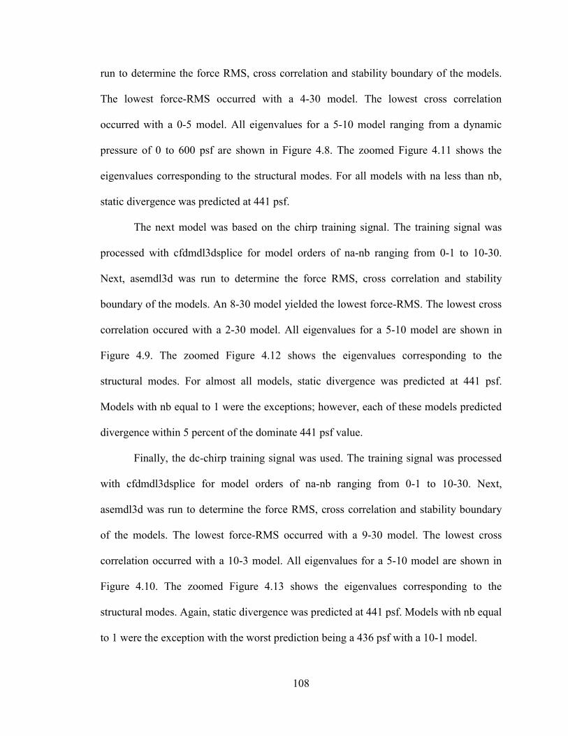
108
run to determine the force RMS, cross correlation and stability boundary of the models.
The lowest force-RMS occurred with a 4-30 model. The lowest cross correlation
occurred with a 0-5 model. All eigenvalues for a 5-10 model ranging from a dynamic
pressure of 0 to 600 psf are shown in Figure 4.8. The zoomed Figure 4.11 shows the
eigenvalues corresponding to the structural modes. For all models with na less than nb,
static divergence was predicted at 441 psf.
The next model was based on the chirp training signal. The training signal was
processed with cfdmdl3dsplice for model orders of na-nb ranging from 0-1 to 10-30.
Next, asemdl3d was run to determine the force RMS, cross correlation and stability
boundary of the models. An 8-30 model yielded the lowest force-RMS. The lowest cross
correlation occured with a 2-30 model. All eigenvalues for a 5-10 model are shown in
Figure 4.9. The zoomed Figure 4.12 shows the eigenvalues corresponding to the
structural modes. For almost all models, static divergence was predicted at 441 psf.
Models with nb equal to 1 were the exceptions; however, each of these models predicted
divergence within 5 percent of the dominate 441 psf value.
Finally, the dc-chirp training signal was used. The training signal was processed
with cfdmdl3dsplice for model orders of na-nb ranging from 0-1 to 10-30. Next,
asemdl3d was run to determine the force RMS, cross correlation and stability boundary
of the models. The lowest force-RMS occurred with a 9-30 model. The lowest cross
correlation occurred with a 10-3 model. All eigenvalues for a 5-10 model are shown in
Figure 4.10. The zoomed Figure 4.13 shows the eigenvalues corresponding to the
structural modes. Again, static divergence was predicted at 441 psf. Models with nb equal
to 1 were the exception with the worst prediction being a 436 psf with a 10-1 model.

109
Figure 4.8 SDOF: Multistep Eigenvalues
Figure 4.9 SDOF: Chirp Eigenvalues
Figure 4.10 SDOF: DC-Chirp Eigenvalues
Figure 4.11 SDOF: Multistep Zoomed
Eigenvalues
Figure 4.12 SDOF: Chirp Zoomed Eigenvalues
Figure 4.13 SDOF: DC-Chirp Zoomed Eigenvalues
In summary, system identification predicts a static divergence at 441 psf for this
single degree of freedom airfoil at Mach 2.0. It is interesting to note that the three training
signal forms predict nearly identical boundary points. The type of training signal has little
influence on the overall solution accuracy because the piston solution aerodynamics are
so simple. It is noticed that the eigenvalues corresponding to the aerodynamics terms are
somewhat different when plotted over a dynamic pressure range; however, the structural
eigenvalues are identical.
Free response simulations are also available to search for the static divergence
dynamic pressure. The actual dynamic pressure for zero torsional stiffness is not
obtainable because the time history will include an increasing larger static offset

110
displacement as dynamic pressure is increased. This is the classic characteristic obtained
for near-divergent time histories. The effective structural and aerodynamic springs are
balanced at ever increasing angles of attack as the aerodynamic spring becomes stiffer. A
time history plot of displacement is shown in Figure 4.14. Any small increment in
dynamic pressure quickly causes the euler3d implementation of the CFD piston solver to
switch to a non-linear base-pressure routine, which, in this case, effectively eliminates the
divergence phenomenon. The final generalized displacement at 411 psf is 0.5, which
corresponds to 5 degrees angle of attack in the physic model.
0 500 1000 1500 2000 2500 3000 3500 4000 4500 50000
0.5
1Displacement
Figure 4.14 SDOF: Free Response at 411 psf
Now, linearized supersonic airfoil theory is used to determine the theoretical static
divergence dynamic pressure. From linearized supersonic airfoil theory, the center of lift
acts at mid-chord with a lift coefficient 14 2 −= MCl α . As derived in Appendix D,
the dynamic pressure for divergence is:
4110
2
3
−= McK
q α
Applying the structural parameters yields a dynamic pressure for divergence of 433 psf.
Divergence boundaries for the theoretical and the system identification model are
within 3 percent of each other. This close result was not expected because the CFD
aerodynamics grid is a “subsonic” NACA 0012.

111
4.2.2 Mach 0.6
The subsonic divergence boundary prediction for the single degree of freedom
airfoil problem is made at Mach 0.6. The static divergence is predicted using both system
identification and linearized aerodynamics.
System training proceeded similarly to the Mach 2.0 case. Six training signals
were used: the 3211 multistep, the chirp, the dc-chirp, the Schroeder sweep, the strictly
specified Fresnel and the state-space Fresnel. The training signals are shown in the
following group of figures:

112
0 0.5 1 1.5 2 2.5 30
0.05
0.1Displacement
0 0.5 1 1.5 2 2.5 3−0.1
−0.05
0
0.05
0.1velocity
0 0.5 1 1.5 2 2.5 3−2
0
2
4x 10
−3 Forces
Figure 4.15 SDOF: Multistep Training
Signal Mach 0.6
0 0.5 1 1.5 2 2.5 3−0.01
−0.005
0
0.005
0.01Displacement
0 0.5 1 1.5 2 2.5 3−0.2
−0.1
0
0.1
0.2velocity
0 0.5 1 1.5 2 2.5 3−4
−2
0
2
4x 10
−3 Forces
Figure 4.16 SDOF: Chirp Training Signal
Mach 0.6
0 0.5 1 1.5 2 2.5 30
0.005
0.01Displacement
0 0.5 1 1.5 2 2.5 3−0.1
−0.05
0
0.05
0.1velocity
0 0.5 1 1.5 2 2.5 3−2
−1
0
1
2x 10
−3 Forces
Figure 4.17 SDOF: DC-Chirp Training
Signal Mach 0.6
0 0.5 1 1.5 2 2.5 3 3.5 4−0.01
−0.005
0
0.005
0.01Displacement
1
0 0.5 1 1.5 2 2.5 3 3.5 4−0.4
−0.2
0
0.2
0.4velocity
1
0 0.5 1 1.5 2 2.5 3 3.5 4−4
−2
0
2
4x 10
−3 Forces
1
Figure 4.18 SDOF: Schroeder Training Signal Mach 0.6
0 0.5 1 1.5 2 2.5 3 3.50
0.02
0.04
0.06
0.08Displacement
1
0 0.5 1 1.5 2 2.5 3 3.5−0.1
−0.05
0
0.05
0.1Velocity
1
0 0.5 1 1.5 2 2.5 3 3.5−1
0
1
2
3x 10
−3 Forces
1
Figure 4.19 SDOF: Strict Fresnel Mach 0.6
0 0.5 1 1.5 2 2.5 3 3.5 40
0.2
0.4Displacement
1
0 0.5 1 1.5 2 2.5 3 3.5 4−1
−0.5
0
0.5
1Velocity
1
0 0.5 1 1.5 2 2.5 3 3.5 4−5
0
5
10
15x 10
−3 Forces
1
Figure 4.20 SDOF: State Space Fresnel
Mach 0.6

113
The first training signal tested is the 3211 multistep. Figure 4.15 shows the
training signal time history for the multistep. The majority of the output force changes
occur near the step changes in velocity. The training signal was processed with
cfdmdl3dsplice for model orders of na-nb ranging from 0-1 to 10-30. The lowest force-
RMS occured with a 2-25 model. The lowest cross correlation occurred with a 6-9 model.
Model order sensitivity is plotted in Figure 4.21. Dynamic pressure is swept from 0 to
200 psi. Static divergence was predicted in a band from 110 psf to 125 psf. Coupled aero-
structural eigenvalues for the multistep input are plotted in Figure 4.27 in the z plane. The
far right points are the eigenvalues associated with the structural motion, while the others
are aerodynamics. An eigenvalue exists at the Nyquist frequency on the unit circle.
The chirp training signal time history is shown in Figure 4.16. The training signal
was processed with cfdmdl3dsplice for model orders of na-nb ranging from 0-1 to 15-60.
The lowest force-RMS occurred with a 1-33 model. The lowest cross correlation
occurred with a 0-13 model. Eigenvalues for a 5-10 model are shown in Figure 4.28. A
damped eigenvalue exists at the Nyquist frequency. Static divergence was predicted
between a band from 100 psf to 130 psf. Model order sensitivity is plotted in Figure 4.22.

114
0 10 20 30 40 50 600
50
100
150
0
1
2
3
4
5
6
789
1011
1213
1415
nb Order
Dyn
amic
Pre
ssur
e
na Order
Figure 4.21 SDOF: Multistep Model Order Sensitivity
0 10 20 30 40 50 600
20
40
60
80
100
120
140
160
180
200
0
1
2
3
456
789101112131415
nb Order
Dyn
amic
Pre
ssur
e
na Order
Figure 4.22 SDOF: Chirp Model Order Sensitivity
0 10 20 30 40 50 600
20
40
60
80
100
120
140
160
180
0
1
2
345678
9101112131415
nb Order
Dyn
amic
Pre
ssur
e
na Order
Figure 4.23 SDOF: DC-Chirp Model Order Sensitivity
0 10 20 30 40 50 600
20
40
60
80
100
120
140
160
180
0
1
nb Order
Dyn
amic
Pre
ssur
e
na Order
No Stability Boundary Found for na>1
Figure 4.24 SDOF: Schroeder Model Order Sensitivity
0 10 20 30 40 50 600
50
100
150
0
1
2
3
456789101112131415
nb Order
Dyn
amic
Pre
ssur
e
na Order
Figure 4.25 SDOF: Strict Fresnel Model Order Sensitivity
0 10 20 30 40 50 600
20
40
60
80
100
120
140
160
180
0
1
2
34
56
7891011121314151617181920
nb Order
Dyn
amic
Pre
ssur
e
na Order
Figure 4.26 SDOF: State-Space Fresnel Model Order Sensitivity
The dc-chirp training signal time history is shown in Figure 4.17. The training
signal was processed with cfdmdl3dsplice for model orders of na-nb ranging from 0-1 to

115
15-60. The lowest force-RMS occurred with a 13-19 model. The lowest cross correlation
occurred with a 1-15 model. Eigenvalues for a 5-10 model are shown in Figure 4.29. The
most striking difference between this dc-chirp and the regular chirp is the difference in
expansion rate for the eigenvalues centered on the origin. This non-physical expansion
causes problems with certain testcases at large dynamic pressures. These eigenvalues are
required to exist; however, it is preferred that they remain near the origin. Model order
sensitivity is plotted in Figure 4.22. Static divergence was predicted at 120 psf.
The Schroeder sweep time history is shown in Figure 4.18. For this testcase, the
Schroeder sweep does not provide an accurate representation of the aeroelastic boundary.
Figure 4.24 shows the model order sensitivity of the Schroeder sweep. No stability
boundary was found for nb greater than 1. Additionally, nb convergence does not occur.
A free response simulation indicates static divergence at all dynamic pressures. This
physically impossible result should not occur. The eigenvalues corresponding to the
Schroeder input signal are given in Figure 4.30. An eigenvalue exists on the real axis
outside the unit circle. This is neither desired nor physical. Otherwise, the Schroeder
input signal produces a preferable eigenvalue structure. The Schroeder sweep excitation
appears to be causing a misidentification of the aerodynamics. This problem seems to be
caused by the Schroeder sweep’s parameter sensitivity as discussed in Simon [2000] .
The PSD of the actual input signal used for this testcase revealed gaps in the frequency
spectrum. These frequency subband gaps are known to cause sensitivities [Simon, 2000].
It is also possible that these sensitivities are being introduced by the envelope term used
to start the input signal from zero initial conditions. Unfortunately, a better method for

116
starting the Schroeder sweep without generating non-physical solution transients is not
known.
A strict motion specified Fresnel chirp training time history is given in Figure
4.19. A model order sensitivity study using na from 0 to 15 and nb from 1 to 60 is plotted
in Figure 4.25. Interestingly, the stability boundary prediction appears to converge until
reaching nb of approximately 50. The higher order models are becoming numerically
unstable. The coupled aeroelastic eigenvalues for a 5-10 model are plotted in Figure 4.31
for a dynamic pressure range from 0 to 200 psi. The eigenvalue structure resembles the
dc-chirp’s.
A state-space motion specified Fresnel chirp time history is given in Figure 4.20.
The ending condition for this training signal is a constant velocity, which creates the
linear displacement response after the non-dimensional time of 3.5. A model order
sensitivity study is shown in Figure 4.24. Model order convergence resembles that of the
dc-chirp. Interestingly, the very low nb model orders have significantly more consistent
predictions for this state-space motion specification than for any of the strict motion
specification models. Eigenvalues for the coupled aeroelastic system with a 5-10 model
order are shown in Figure 4.32. An eigenvalue near the Nyquist frequency has appeared.
Also, the near-origin eigenvalue structure is rotated by 45 degrees when compared to the
strict motion specification forms.

117
−1 −0.5 0 0.5 1−1
−0.8
−0.6
−0.4
−0.2
0
0.2
0.4
0.6
0.8
1
Real(z)
Imag
(z)
Figure 4.27 SDOF: Multistep
Eigenvalues Mach 0.6
−1 −0.5 0 0.5 1−1
−0.8
−0.6
−0.4
−0.2
0
0.2
0.4
0.6
0.8
1
Real(z)
Imag
(z)
Figure 4.28 SDOF: Chirp Eigenvalues
Mach 0.6
−1 −0.5 0 0.5 1−1
−0.8
−0.6
−0.4
−0.2
0
0.2
0.4
0.6
0.8
1
Real(z)
Imag
(z)
Figure 4.29 SDOF: DC-Chirp
Eigenvalues Mach 0.6
−1 −0.5 0 0.5 1−1
−0.8
−0.6
−0.4
−0.2
0
0.2
0.4
0.6
0.8
1
Real(z)
Imag
(z)
Figure 4.30 SDOF: Schroeder
Eigenvalues Mach 0.6
−1 −0.5 0 0.5 1−1
−0.8
−0.6
−0.4
−0.2
0
0.2
0.4
0.6
0.8
1
Real(z)
Imag
(z)
Figure 4.31 SDOF: Strict Fresnel
Eigenvalues Mach 0.6
−1 −0.5 0 0.5 1−1
−0.8
−0.6
−0.4
−0.2
0
0.2
0.4
0.6
0.8
1
Real(z)
Imag
(z)
Figure 4.32 SDOF: State Space Fresnel
Eigenvalues Mach 0.6

118
Linearized airfoil theory is used to determine the theoretical static divergence
dynamic pressure. From linearized subsonic airfoil theory, the center of lift acts at
quarter-chord with a lift coefficient 212 MCl −= πα . The dynamic pressure for
divergence is:
πα
21
320 2
3
McK
q −=
This yields a dynamic pressure for static divergence of 92 psf.
4.3 AGARD 445.6
The AGARD 445.6 testcase presents an aeroelastic structure typical of high
performance aircraft. Aeroelastic characteristics were measured at subsonic and
supersonic Mach numbers. The experiments were conducted in the 1960’s at NASA
Langley [Yates, 1987].
The AGARD structure consists of a cantilevered wing constrained at the root. The
wing has an aspect ratio of 4.0, a quarter chord sweep of 45 degrees and a taper ratio of
0.6. The airfoil is a NACA 65A004. A planform view of the wing with the CFD
tetrahedral mesh is shown in Figure 4.33. The modeshapes and frequencies are shown in
Figure 4.34.

119
Root
Tip
V
Figure 4.33 AGARD: Planform
Mode 1 at 9.6 Hertz
Mode2 at 38.2 Hertz
Figure 4.34 AGARD: Modeshapes
4.3.1 Flutter Boundary
An experimental flutter boundary for the AGARD is reported in [Yates 1987] and
is reproduced in Table 4.3. The actual model description for the AGARD testcase under
consideration is the wall-mounted 2.5 foot span, weakened model #3 tested in air. The
boundary is reported as a flutter speed index instead of dynamic pressure. The
experimental data does not contain any sensitivity or experimental uncertainty
information.
Mach Number
Flutter Speed Index
Dynamic Pressure [psi]
0.499 0.446 0.924 0.678 0.417 0.807 0.900 0.370 0.636 0.960 0.308 0.441 1.072 0.320 0.476 1.141 0.403 0.754
Table 4.3 AGARD 445.6: Experimental Flutter Boundary
The system identification flutter boundary for the AGARD was computed over
the experimental Mach number range with multiple training signals and training

120
methodologies. Corresponding free response simulations evaluated the system
identification predictions for the coupled CFD-structural aeroelastic system.
It is important to remember that the overall objective is to replace the CFD flow
solver with a state space model. Thus, the relevant flutter boundary comparison is
between the CFD and ARMA boundaries not between the ARMA and experimental
boundaries. The objective is for the ARMA model to match the CFD boundary. Because
the structural and aerodynamic grids are not fully converged, it is expected that
differences will occur between the computational and experimental boundaries. Failure to
match experimental data does not indicate failure of the system identification routine.
4.3.1.1 Training Signal Investigation at Mach 0.90
A detailed training signal investigation was performed for the AGARD at Mach
0.90. The flow solution at Mach 0.90 has a shock on the aft outboard portion of the
AGARD wing. The signals investigated are the multistep, chirp, dc-chirp, Schroeder
sweep and the Fresnel chirp.
The multistep sensitivity plot is given in Figure 4.35. The maximum training
modal deflection was 0.5. The system converges with increases in both na and nb orders.
The ARMA predicted flutter boundary is 0.48 psi. The CFD boundary is 0.62 psi. This is
a 23 percent difference error.

121
0 5 10 15 20 25 300
0.1
0.2
0.3
0.4
0.5
0.6
0.7
0
1
23456
7891011121314151617181920
nb Order
na Order
0.636 Experiment
Dynamic Pressure [psi]
Figure 4.35 AGARD: Multistep Sensitivity
The chirp sensitivity plot is given in Figure 4.36. The maximum training
displacement was 0.2. The predictions converge for na>1 and nb>5. The converged
ARMA prediction is 0.59 psi. This is a 5 percent difference error. The stability boundary
prediction decreases after the initial convergence point. This appears to indicate that
better low frequency excitation would be advantageous.
0 5 10 15 20 25 300
0.1
0.2
0.3
0.4
0.5
0.6
0.7
0.8
0.9
1
0
1 234567891011121314151617181920
nb Order
Dynamic Pressure [psi]
na Order
0.636 Experiment
Figure 4.36 AGARD: Chirp Sensitivity

122
The dc-chirp sensitivity plot, Figure 4.37, shows improved results. The dc-chirp
was trained with displacements of 0.5. Convergence occurs for nb>5 and na>0 and is
consistent across the entire range of na and nb. Better still, the final dynamic pressure
prediction is 0.62 psi. There is effectively no error when compared to the CFD free
response. An increase in the input signal’s low frequency power seems to have
significantly improved the prediction performance.
0 5 10 15 20 25 300
0.1
0.2
0.3
0.4
0.5
0.6
0.7
0.8
0
1 234567891011121314151617181920
nb Order
na Order
0.636 Experiment
Dynamic Pressure [psi]
Figure 4.37 AGARD: DC-Chirp Sensitivity
Increasing the displacement to 4 and 3 units for mode 1 and 2, respectively, yields a
similar, but not quite as converged, flutter boundary. The flow conditions are becoming
nonlinear. The sensitivity plot is given in Figure 4.38. The best prediction appears to be
0.6 psi or approximately 3 percent difference error.
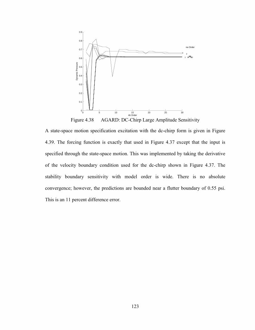
123
0 5 10 15 20 25 300
0.1
0.2
0.3
0.4
0.5
0.6
0.7
0.8
0.9
0
1
2
345678910
nb Order
Dyn
amic
Pre
ssur
e
na Order
Figure 4.38 AGARD: DC-Chirp Large Amplitude Sensitivity
A state-space motion specification excitation with the dc-chirp form is given in Figure
4.39. The forcing function is exactly that used in Figure 4.37 except that the input is
specified through the state-space motion. This was implemented by taking the derivative
of the velocity boundary condition used for the dc-chirp shown in Figure 4.37. The
stability boundary sensitivity with model order is wide. There is no absolute
convergence; however, the predictions are bounded near a flutter boundary of 0.55 psi.
This is an 11 percent difference error.

124
0 5 10 15 20 25 30 35 400
0.1
0.2
0.3
0.4
0.5
0.6
0.7
0.8
0.9
1
0
1
2
3
4567
8
910
1112
1314151617
181920
nb Order
Dyn
amic
Pre
ssur
e
na Order
Figure 4.39 AGARD: DC-Chirp State Space Methodology Sensitivity
The Schroeder sweep sensitivity plot is given in Figure 4.40. Convergence occurs
but at a slow rate. The best-converged prediction occurs at 0.50 psi or 20 percent
difference error. Overall, the Schroeder gave worse aeroelastic predictions than even the
multistep.
0 5 10 15 20 25 300
0.2
0.4
0.8
1
1.2
1.4
1.6
1.8
0 1
2
3
4
5
67
8
910
111213
14151617181920
nb Order
na Order
0.636 Experiment
Dynamic Pressure [psi]
Figure 4.40 AGARD: Schroeder Sweep Sensitivity

125
The Fresnel chirp sensitivity plot is shown in Figure 4.41. This training signal is
based on a state-space motion specification. The predictions appear to converge to
0.54 psi. This is 13 percent difference error.
0 10 20 30 40 50 600
0.1
0.2
0.3
0.4
0.5
0.6
0.7
0.8
0.9
0
1
2
3
4567891011121314151617181920
nb Order
Dyn
amic
Pre
ssur
e
na Order
Figure 4.41 AGARD: Fresnel Sensitivity
This training signal sensitivity study shows some interesting results. First, adding
low frequency information to the input signal significantly improves the stability
boundary prediction. This improvement, which is due to additional low frequency power,
was predicted. Second, it is interesting that the state-space motion specification
performed worse than the strict motion specification for the AGARD at Mach 0.90. This
result does not agree with the hypothesis and prediction given in section 3.3.12. The third
interesting result is the importance of smooth higher-order derivative excitation as shown
by comparing the multistep prediction with the other predictions.
4.3.1.2 Mach Number Flutter Boundary
The flutter boundary results across the experimental Mach range are shown in
Figure 4.42. The solid line plots the estimated experimental flutter boundary presented by

126
Yates. The free response boundary is shown as circles, ○. The system identification
boundary is given by stars, *. A free response boundary was not performed at Mach
1.072. For subsonic flow conditions, both the system identification and the free response
solutions are within 10% of the experimental results. Uncertainty analysis was not
presented in Yates, so this excellent prediction fit might be misleading. Still, it must be
stated that the computational predictions are presented without individual tweaking. The
same simulation process, input data files and CFD parameters were used across the entire
Mach range.
0.4 0.5 0.6 0.7 0.8 0.9 1 1.1 1.20
0.2
0.4
0.6
0.8
1
1.2
1.4
1.6
1.8
Mach Number
Dyn
amic
Pre
ssur
e [p
si]
Figure 4.42 AGARD: Flutter Boundary
The flutter boundary results contain two interesting points. First, the system
identification process accurately predicts the stability boundary when compared to the
CFD solver. Second, the two mode structural assumption appears to become invalid for
supersonic flows. Gordnier [2000] confirms this hypothesis with a mode shape sensitivity
study at Mach 1.141. The flutter boundary decreased as the number of structural modes
increased. Regardless of the comparisons between the computational and experimental
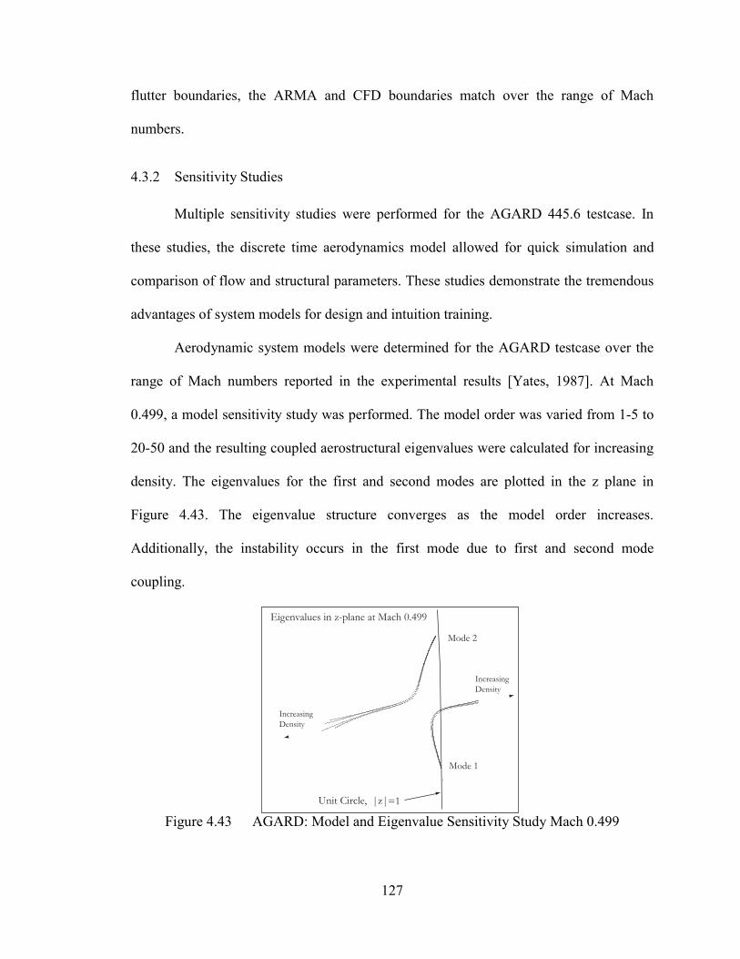
127
flutter boundaries, the ARMA and CFD boundaries match over the range of Mach
numbers.
4.3.2 Sensitivity Studies
Multiple sensitivity studies were performed for the AGARD 445.6 testcase. In
these studies, the discrete time aerodynamics model allowed for quick simulation and
comparison of flow and structural parameters. These studies demonstrate the tremendous
advantages of system models for design and intuition training.
Aerodynamic system models were determined for the AGARD testcase over the
range of Mach numbers reported in the experimental results [Yates, 1987]. At Mach
0.499, a model sensitivity study was performed. The model order was varied from 1-5 to
20-50 and the resulting coupled aerostructural eigenvalues were calculated for increasing
density. The eigenvalues for the first and second modes are plotted in the z plane in
Figure 4.43. The eigenvalue structure converges as the model order increases.
Additionally, the instability occurs in the first mode due to first and second mode
coupling.
Eigenvalues in z-plane at Mach 0.499
Unit Circle, |z|=1
Mode 2
Mode 1
Increasing
Density
Increasing
Density
Figure 4.43 AGARD: Model and Eigenvalue Sensitivity Study Mach 0.499
128
Next, a Mach number sensitivity study was performed. In this study, the effects of
Mach number are investigated for the first mode structural eigenvalues. Figure 4.44 plots
the eigenvalues corresponding to the first structural mode as dynamic pressure increases
at six Mach numbers. The transonic flutter boundary dip seen in the experimental
boundary is explained by a decrease in first mode aerodynamic damping. The
aerodynamic damping increases as Mach number increases beyond Mach 0.96. However,
the eigenvalues stay near the unit circle. For supersonic Mach numbers, structural
damping dominates the location of the stability boundary. From Figure 4.44, the effective
damping follows the unit circle closer as Mach number is increased. At the lower Mach
numbers, a pronounced damping dip occurs before the eigenvalues cross the unit circle
almost perpendicularly. At the higher Mach numbers, the damping dip is less and the
crossing is more acute. This indicates that regardless of the eventual crossing dynamic
pressure, the AGARD at supersonic Mach numbers will always be just marginally stable.
This has sensitivity implications for wind tunnel testing.
1.141 1.072
0.499
0.6780.900
0.960
|z|=1 Figure 4.44 AGARD: Mach Number and Eigenvalue Sensitivity Study
To investigate the sensitivity that structural damping imparts on the AGARD stability
boundary, a sensitivity study was performed at Mach 0.499 and 1.072 for variable

129
structural damping. The eigenvalues for a density sweep were evaluated at damping
ratios of { }%16%8%4%2%1%0=ζ . Figure 4.45 displays the eigenvalues for
the first mode. Figure 4.46 displays the dynamic pressure for the stability boundary
versus damping ratio for the two Mach numbers. The supersonic flow provides little
aerodynamic damping when compared to the subsonic case. Adding structural damping
to the supersonic case appears to have little effect on the frequency.
Mach 0.499 Mach 1.072
Figure 4.45 AGARD: Damping Sensitivity at Mach 0.499 and 1.072
0 2 4 6 8 10 12 14 160.7
0.75
0.8
0.85
0.9
0.95
1
1.05
1.1
Damping Ratio %
Stability Boundary [psi]
Mach 0.499
Mach 1.072
Figure 4.46 AGARD: Damping Sensitivity
A sensitivity study on structural frequency was performed. The free vibration frequency
was modified plus and minus 10% through the modal stiffness while the modal mass
remained constant. This simulates the error occurring due to material inconsistencies and
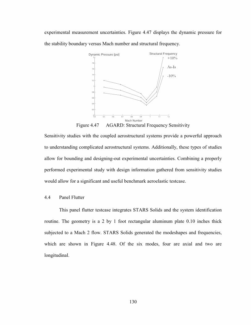
130
experimental measurement uncertainties. Figure 4.47 displays the dynamic pressure for
the stability boundary versus Mach number and structural frequency.
0.4 0.5 0.6 0.7 0.8 0.9 1 1.1 1.20
0.2
0.4
0.6
0.8
1
1.2
1.4
1.6
1.8
2
Mach Number
Dynamic Pressure [psi]+10%
-10%
As-Is
Structural Frequency
Figure 4.47 AGARD: Structural Frequency Sensitivity
Sensitivity studies with the coupled aerostructural systems provide a powerful approach
to understanding complicated aerostructural systems. Additionally, these types of studies
allow for bounding and designing-out experimental uncertainties. Combining a properly
performed experimental study with design information gathered from sensitivity studies
would allow for a significant and useful benchmark aeroelastic testcase.
4.4 Panel Flutter
This panel flutter testcase integrates STARS Solids and the system identification
routine. The geometry is a 2 by 1 foot rectangular aluminum plate 0.10 inches thick
subjected to a Mach 2 flow. STARS Solids generated the modeshapes and frequencies,
which are shown in Figure 4.48. Of the six modes, four are axial and two are
longitudinal.

131
Figure 4.48 Panel: Modeshapes and Frequencies
The euler3d CFD solver uses the finite element grid shown in Figure 4.49. The 2 by 1
plate resides in the finely resolved center of the CFD grid.
Figure 4.49 Panel: CFD Grid
The flow enters the grid on the left hand side of Figure 4.49. To capture the convection,
the downstream portion of the grid is refined.

132
4.4.1 Serial Chirp Training
The traditional system identification process evaluates the system response based
on a continuous series of input signals. All modes are trained during the same CFD run.
The training signal is a frequency-sweep modified chirp. The chirp is based on the
composition of a harmonic function and an envelope function. The sweep rate is specified
by the harmonic function. The highest sweep frequency is based on the envelope
function. Their combination specifies the signal duration.
The panel testcase required six chirps, one for each mode. The chirps are applied
one after the other, as shown in Figure 4.50. For each subplot of displacement, velocity
and force, there are 6 time-history traces, one for each mode.
Figure 4.50 Panel: Serial Training Signal
From the training signal, ARMA models are determined using cfdmdl3d. The
models are verified by forced response simulations, which ensure that the ARMA
predicted forces agree with the actual CFD forces for a 2-7 model. Figure 4.51 shows the

133
actual forces as lines and the ARMA predictions as dots. The predicted forces lie on the
actual forces for all six modes.
The aeroelastic boundaries predicted by asemdl3d are consistent at a density of
0.0163 slug·ft-3. Figure 4.52 shows the resulting coupled aero-structural eigenvalues.
Figure 4.51 Panel: 2-7 Model ARMA Predictions
Figure 4.52 Panel: Eigenvalues
The third mode exits the unit circle first. This result is surprising because traditional 2D
panel flutter theory predicts that dynamic instabilities first occur in modes 1 and 2.
Significant coupling occurs for modes 1 and 2 but the combination does not become
unstable.
For this serial method, the training signal required 290 time units for a solution.
Any disruptions in the training signal, such as a power outage, require the entire signal to
be regenerated from the beginning. For larger problems with more modes, the time
required for a single serial training signal may be weeks or months. This training method
appears to be suboptimal and overly sensitive to possible glitches.

134
4.4.2 Parallel Chirp Training
The parallel system identification process evaluates the system response based on
a separate series of input signals. Each mode is trained during separate CFD runs.
The training signal uses the chirp; however, only one mode is excited per CFD
run. For the plate testcase, six individual runs were made. The six training signals are
plotted in Appendix G.
The six separate training signals are spliced together to form one combined
training signal for the entire testcase. Figure 4.53 shows the six separately numbered
xn.dat files rejoined as one large xn.dat file. The vertical lines indicate the splice points
and the corresponding mode. This file exactly matches the serial training signal.
Figure 4.53 Panel: Parallel Training Signal
As before, ARMA models are fit to the training data. The models and boundary
predictions for this parallel method are identical to the serial method given in the
preceding section. An aeroelastic boundary is found at a density of 0.0163 slug·ft-3. The

135
flutter prediction for the parallel calculation method is exactly the same as the serial
method.
The parallel method allows for a speed increase equal to the number of structural
modes. In this plate test case, each parallel chirp required 47 time units for a total of 282
units of total computation time spread over 6 computers. The serial method requires a
calculation time of 290 units. The timesavings will be even larger for a greater number of
modes. In addition, the training for a given mode may be done at any time and added to
the overall time history as needed without the requirement for running the entire
simulation again.
4.4.3 Free Response Aeroelastic Boundary Validation
The aeroelastic boundary was validated with aero-structure coupled free response
runs. The starting dynamic pressure for this free response validation was determined from
the system identification aeroelastic boundary. Figure 4.54 plots the displacement time
history for a free response with a free stream density of ρ=0.0160 slug·ft-3. This response
is stable.
Figure 4.54 Panel: Free Response at ρ=0.0160 slug·ft-3.
Figure 4.55 plots the displacement time history for a free response with a free stream
density of ρ=0.0163 slug·ft-3. This response is neutrally stable.

136
Figure 4.55 Panel: Free Response at ρ=0.0163 slug·ft-3.
Figure 4.56 plots the displacement time history for a free response with a free stream
density of ρ=0.0166 slug·ft-3. This response is unstable.
Figure 4.56 Panel: Free Response at ρ=0.0166 slug·ft-3.
The free response boundary exactly corresponds to the system-identification
boundary of 0.0163 slug·ft-3. Each free response required approximately 150 units of
time. For the three free responses shown here, the total time was 450 units. Typically, a
search requires significantly more time because an estimated dynamic pressure for flutter
is not available. The traditional free response always will find the stability boundary;
however, the free response search might require significantly more time that a
corresponding system identification search.
4.5 Wing/Flap Control
The general testcase geometry is a two-dimensional wing with a trailing edge control
flap. The entire wing is elastically restrained about an upstream rotation point. The
generalized geometry is shown in Figure 4.57.

137
U
θδ
D eL
Figure 4.57 Wing-Flap: Geometry
4.5.1 Aerodynamic and Structural Representations
The first step with CFD was to create a representation of the flow geometry. A
NACA 0012 airfoil testcase was selected. The CFD grid is given in Figure 4.58.
Significant refinement occurs aft of the airfoil. This was done to capture the
aerodynamics resulting from the shed wake. The grid contains 235-thousand elements.
Figure 4.58 Wing-Flap: CFD Grid
Next, modeshapes corresponding to the wing rotation and the flap control mode
were created with transpiration. The modeshapes are not easily visualized with the CFD
grid. Refer to Figure 4.57 for a schematic view of the modeshapes. Both the wing rotation
and flap deflection modeshapes have a unit deflection of 1 degree.

138
4.5.2 Training
Aerodynamic training data was generated in parallel with the offset dc-chirp. The
chirp frequency swept from zero to 10 percent of Nyquist. Each of the two modes was
individually excited to generate the following two training time histories. Figure 4.59
shows the training time history for the first mode, rotation angle. The figure displays
displacement, velocity and two modal forces. Velocity effects dominate the first mode
force. Second mode forces are almost hidden by the order of magnitude larger first mode
forces; however, the training signal did excite forces in both modes.
0 5 10 15 20 25 30 350
0.5
1
1.5
2Displacement
12
0 5 10 15 20 25 30 35−20
−10
0
10
20Velocity
12
0 5 10 15 20 25 30 35−0.01
−0.005
0
0.005
0.01Forces
12
Figure 4.59 Wing-Flap: Mode 1 Training
0 5 10 15 20 25 30 350
0.5
1
1.5
2Displacement
12
0 5 10 15 20 25 30 35−20
−10
0
10
20Velocity
12
0 5 10 15 20 25 30 35−2
0
2
4x 10
−4 Forces
12
Figure 4.60 Wing-Flap: Mode 2 Training
Training for the second mode is shown in Figure 4.60. Again, the chirp was swept
to 10 percent of Nyquist. The resulting forces due to second mode excitation include
more complex aerodynamics than the first mode. The smaller magnitude symmetrical
output force is the second mode. The flap produces a symmetrical hinge moment
dominated by velocity. Wing moment produced by the flap is clearly dominated by flap
displacement; however, velocity effects are also apparent. A slight perturbation in the
output force occurs between time 5 and 15. This appears to be caused by excitation
pressure waves moving upstream. This bump in the force plot might represent an

139
unsteady pressure distribution effect similar to the Sears problem. Higher frequency
pressure waves appear to be less disruptive.
4.5.3 Controls
The Ricatti method for control gain selection was investigated for this testcase.
System identification and the Ricatti method chosen do not automatically mesh smoothly.
Ricatti assumes state feedback. In the ARMA model, the states contain aerodynamic
forces, which are not available in reality. Those tempted to use a state observer will also
encounter difficulties because the overall ARMA model is controllable, but not
observable. The difficulty lies in not being able to determine the generalized forces from
the output motion. This is analogous to not being able to deduce a unique flow field from
previous motions. The Ricatti method in this form does not appear to be a good choice
for determining control gains with an ARMA model.
In spite of these problems, the Ricatti method was used to find control gains for
the SDOF testcase. This assumes that all states are known so that a solution, regardless of
its applicability, can be found. The Q matrix from the analytical experiment was used;
however, the Ricatti solution requires a positive definite R matrix. This requirement
forced the R matrix to contain limitation data for all inputs, not just the desired flap
deflection angle. To alleviate this problem, the R matrix weighting for non-flap inputs
were set to large magnitudes. Thus, the final 22 by 6 gain matrix only applied inputs into
the flap deflection angle. Figure 4.61 shows the absolute value of the gains for the couple
aero-elastic state vector as determined with the Ricatti solution method. The motion gains
are:
k={2.029, 0.13197, 0.12102, 0.00783}

140
The flap deflection input is:
flapwingflapwinginput δθδθδ && ⋅+⋅+⋅+⋅= 008.0121.0132.003.2
The motion terms are well behaved. Flap angle inputs are dominated by the wing pitch
angle. The control gains for the actual flap angle is an order of magnitude smaller than
wing angle. This is expected and was seen before in the analytical Ricatti solution above.
However, the aerodynamic gains are problematic. First, it would be preferred if these
gains were zero. Second, the gains have large differences in magnitude with oscillating
phase. This indicates an unusually large sensitivity to the aerodynamics.
103
10 2
10 1
100
101
102
103
104
MotionTerms
AerodynamicTerms
--- + +
Gain Magnitudes
Model Coefficient Location Figure 4.61 Wing-Flap: Ricatti Gains
Overall, the Ricatti method for gain determination did not work well with this
ARMA system model. To even find a solution, several questionable modifications were
made to the standard Ricatti approach. Regardless of these modifications, the resulting
gains still contain fundamental errors when coupled with the ARMA system model.
The control gain selection method that did work was the guess-and-test method. The open
loop system was made to dynamically diverge by adjusting dynamic pressure. The open
loop time history response is given in Figure 4.62.
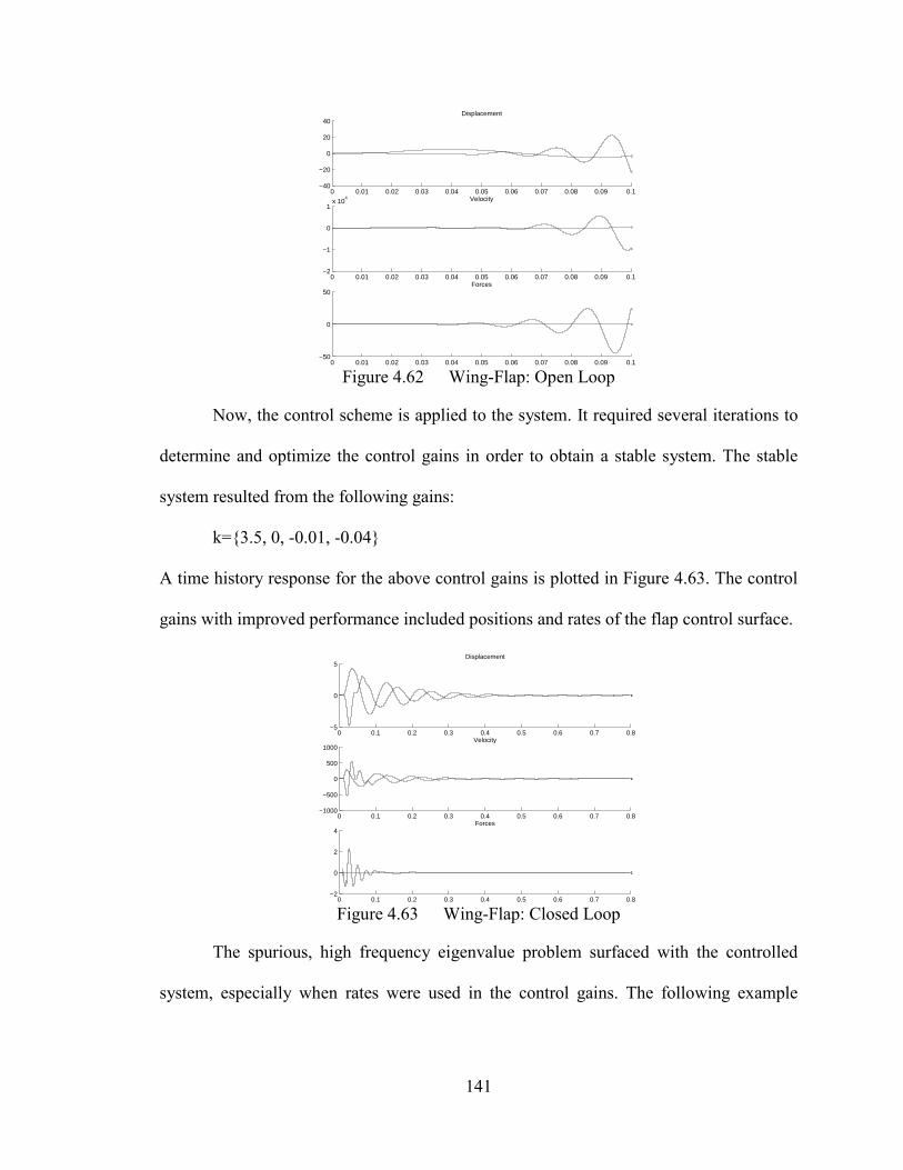
141
0 0.01 0.02 0.03 0.04 0.05 0.06 0.07 0.08 0.09 0.1−40
−20
0
20
40Displacement
1
2
0 0.01 0.02 0.03 0.04 0.05 0.06 0.07 0.08 0.09 0.1−2
−1
0
1x 10
4 Velocity
1
2
0 0.01 0.02 0.03 0.04 0.05 0.06 0.07 0.08 0.09 0.1−50
0
50Forces
1
2
Figure 4.62 Wing-Flap: Open Loop
Now, the control scheme is applied to the system. It required several iterations to
determine and optimize the control gains in order to obtain a stable system. The stable
system resulted from the following gains:
k={3.5, 0, -0.01, -0.04}
A time history response for the above control gains is plotted in Figure 4.63. The control
gains with improved performance included positions and rates of the flap control surface.
0 0.1 0.2 0.3 0.4 0.5 0.6 0.7 0.8−5
0
5Displacement
12
0 0.1 0.2 0.3 0.4 0.5 0.6 0.7 0.8−1000
−500
0
500
1000Velocity
12
0 0.1 0.2 0.3 0.4 0.5 0.6 0.7 0.8−2
0
2
4Forces
12
Figure 4.63 Wing-Flap: Closed Loop
The spurious, high frequency eigenvalue problem surfaced with the controlled
system, especially when rates were used in the control gains. The following example

142
shows the same system made stable with the similar control gains; however, the
unwanted eigenvalues eventually cause non-physical dynamic divergence. The gains are:
k={3.5, 0, -0.01, -0.05}.
This gain represents only a small increase in the flap velocity control gain when
compared to the previous control gain. The previous control gain was numerically stable;
this control gain is not stable. The time history and eigenvalues are given in Figure 4.64
and Figure 4.65. Zooming into Figure 4.64 shows that the diverging chatter occurs at the
Nyquist frequency. The control method is working, but the aerodynamic system model
fails to accurately represent reality. Figure 4.65 shows this and other unwanted spurious
eigenvalues distributed around the unit circle. This spurious eigenvalue topic is discussed
in sections 3.3.11 and 3.3.12.
0 0.02 0.04 0.06 0.08 0.1 0.12 0.14 0.16 0.18 0.2−1
−0.5
0
0.5
1Displacement
12
0 0.02 0.04 0.06 0.08 0.1 0.12 0.14 0.16 0.18 0.2−1
−0.5
0
0.5
1x 10
8 Velocity
1
2
0 0.02 0.04 0.06 0.08 0.1 0.12 0.14 0.16 0.18 0.2−2
−1
0
1
2x 10
8 Forces
1
2
Figure 4.64 Wing-Flap: Closed Loop Chatter Time History
−1 −0.5 0 0.5 1−1
−0.8
−0.6
−0.4
−0.2
0
0.2
0.4
0.6
0.8
1
Figure 4.65 Wing-Flap: Closed Loop Chatter Eigenvalues

143
CHAPTER 5
5CONCLUSIONS AND RECOMMENDATIONS
5.1 Conclusions
This thesis was concerned with improved system identification for CFD based
aeroservoelastic predictions. The system identification routine was decomposed into
major areas for further study. These areas are system theory, training method and
excitation signals. Improvements were made in all three areas. These improvements
allow less sensitive, faster and more precise predictions. Additionally, a figure of merit
investigation was performed to identify useful model selection routines. Various
aeroelastic configurations were tested to evaluate the improvements and identify further
improvements. The results show that the new system identification techniques give
improved aeroservoelastic predictions.
The system theory section investigated aerodynamic models in relation to linear
systems and the CFD solver. The first important result was the insight that the CFD
solver updates the boundary condition states simultaneously. This has important
implications for excitation signal selection. A set of aerodynamic specific requirements
gives a set of guidelines for system identification models. A canonical form for the
ARMA model was developed.
The training method section investigated the methodology used to generate
system models from raw input training data. The identification data flow is charted. A

144
data redundancy criterion is developed to correlate model size with training data size
requirements. The most important result from this section is the development of a true
parallel training scheme. Parallel training allows for decoupled distributed training of
multiple mode systems, which allows for significant increases in training performance.
The excitation signal section investigated signals for aerodynamic training.
Training signal criteria were formed to assist with selection and development of new
signals. The multistep signals were reviewed and found to have undesirable traits. A new
class of analytic signals based on frequency swept chirps was developed. The high and
low frequency power spectral density of input signal was found to be important. Low
frequency power improves coupled aerostructural prediction accuracy. High frequency
power ensures a physically consistent transfer function, which improves aeroservoelastic
predictions. State-space motion specification did not provide better aeroelastic
predictions when compared to strict motion specification.
Summarizing the results of this thesis shows that improvements were made in
aeroservoelastic prediction quality. This research suggests that further improvements in
linear system models will allow better aerodynamic predictions without resorting to
exotic and less-intuitive non-linear techniques.
5.2 System Identification Recommendations
The results of this thesis advocate the following system identification
methodologies. Use the classical ARMA realization (section 3.1.5). Use parallel training
with the true splice functionality given in cfdmdl3d (section 3.2.7.3). The best excitation
signal is the dc-chirp without an envelope (section 3.3.5). The excitation should remain
harmonic; end the CFD simulation without ending the excitation. Size the excitation

145
parameters based on the Nyquist frequency and the model over-determination factor
(sections 3.2.3 and 3.2.4). If needed, add white noise to the excitation signal after training
to improve the system’s transfer function (section 3.3.11). Evaluate the model fit with the
force prediction RMS (section 3.4.2). Evaluate the effective model quality with the
coupled aeroelastic stability boundary and eigenvalues (section 3.4.4). It is essential to
ensure total simulation convergence of the solution residuals, timestep, structural modes
and CFD grid (section 4.1).
5.3 Recommendations for Further Study
This thesis has investigated aeroservoelastic predictions. Multiple promising areas
of research were found, but not investigated. The following topics are recommended for
further study.
5.3.1 Linear System Theory
The underlying fundamental for aeroelastic predictions is learning more about
linear system theory and applying those theories to unsteady aerodynamics. Generally,
what do we know about unsteady aerodynamics, and how can this be incorporated into
the identification, training and prediction routine?
One guiding assumption has been that the aerodynamics can be considered linear
within certain bounds. This assumption has not been investigated with much vigor, yet it
potentially has significant implications for future developments. How linear are our
typical aerodynamics in the range that we consider? How do CFD unsteady results
compare with the classical and fundamental unsteady developments such as Wagner,
Theodorsen and Sears? Can these classical unsteady results be describabled by linear
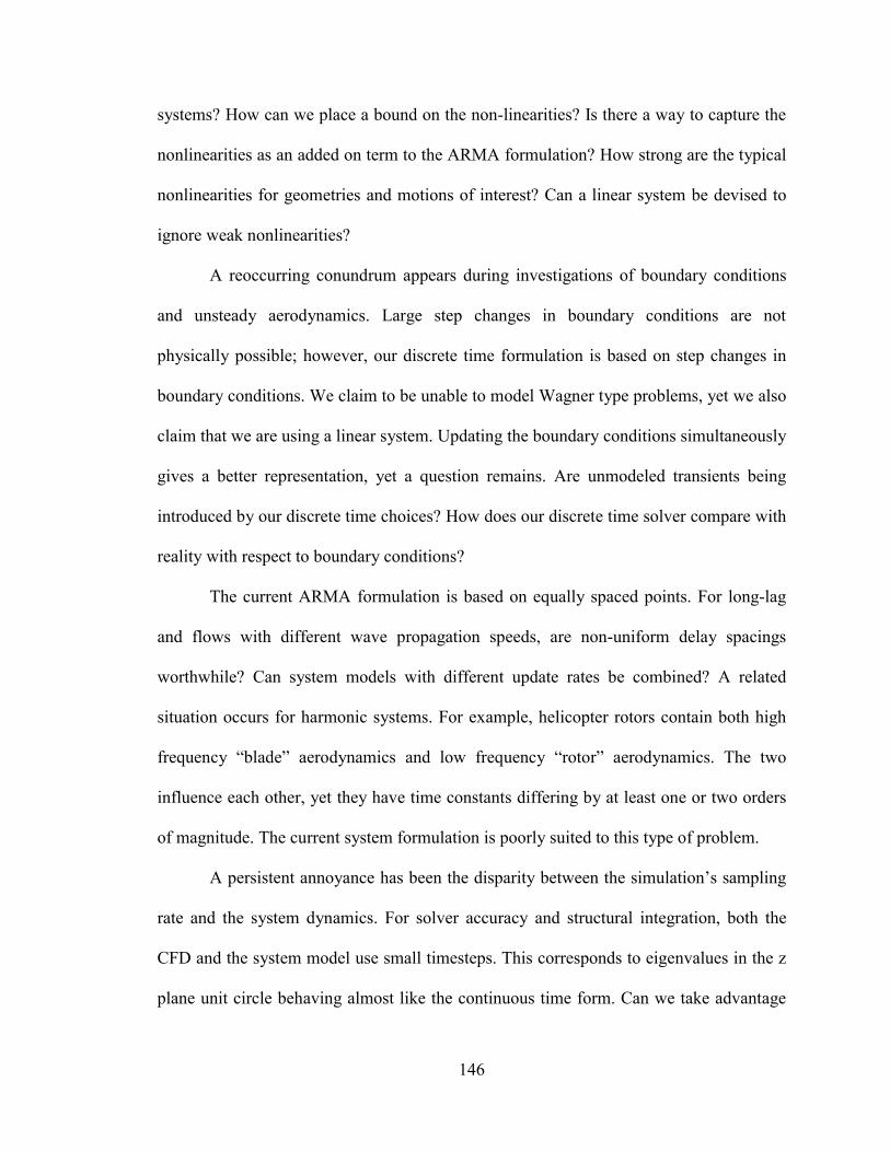
146
systems? How can we place a bound on the non-linearities? Is there a way to capture the
nonlinearities as an added on term to the ARMA formulation? How strong are the typical
nonlinearities for geometries and motions of interest? Can a linear system be devised to
ignore weak nonlinearities?
A reoccurring conundrum appears during investigations of boundary conditions
and unsteady aerodynamics. Large step changes in boundary conditions are not
physically possible; however, our discrete time formulation is based on step changes in
boundary conditions. We claim to be unable to model Wagner type problems, yet we also
claim that we are using a linear system. Updating the boundary conditions simultaneously
gives a better representation, yet a question remains. Are unmodeled transients being
introduced by our discrete time choices? How does our discrete time solver compare with
reality with respect to boundary conditions?
The current ARMA formulation is based on equally spaced points. For long-lag
and flows with different wave propagation speeds, are non-uniform delay spacings
worthwhile? Can system models with different update rates be combined? A related
situation occurs for harmonic systems. For example, helicopter rotors contain both high
frequency “blade” aerodynamics and low frequency “rotor” aerodynamics. The two
influence each other, yet they have time constants differing by at least one or two orders
of magnitude. The current system formulation is poorly suited to this type of problem.
A persistent annoyance has been the disparity between the simulation’s sampling
rate and the system dynamics. For solver accuracy and structural integration, both the
CFD and the system model use small timesteps. This corresponds to eigenvalues in the z
plane unit circle behaving almost like the continuous time form. Can we take advantage

147
of the fact that the interesting aeroelastic results occur at comparatively low frequencies?
Would converting to an actual continuous time form be advantageous?
5.3.2 Training Methodology
This thesis also investigated training methodologies including excitation signals.
The following topics appear to be worth further investigation.
The current SVD solver is a stock solution routine. Different methodologies based
on the SVD are claimed to result in better SVD solutions; however, most require
additional statistical information about the SVD data inputs. Is a weighted or correlated
SVD worth the extra effort? Can we use Mahalanobis-distance minimization techniques?
Would normalizing the SVD inputs reduce magnitude scale errors? Would a Total-Least-
Squares or a related methodology assist in more precise model selection?
The current methodology uses a direct approach to determine system coefficients.
It appears that the transfer function directly out of the CFD solution matches the
dominate physics better than the transfer function out of the corresponding ARMA
model. Would forcing the ARMA model to fit a specified transfer function improve the
overall model quality? Could fitting the training data to a transfer function, and then
transforming back, result in less sensitive models? Ljung [1987] and others advocate
frequency domain approaches. Any attempt at this method will encounter the difficulties
caused by frequency domain estimation problems with harmonic windowing.
Input signal sensitivities appear much larger than expected. Small changes in
input signal often cause dramatic changes in model quality. Does this indicate that the
training signals still do not fully excite all of the dynamics? Can the general harmonic
Schroeder problem be solved for arbitrary phasing? How does input signal selection

148
change with the presence of nonlinear physics? Why did state-space motion specification
give poor results? Theory predicted state-space specification would be an improvement
over strict motion specification. Does non-analytic motion specification practically
require more than displacement state information?
Input-output noise was shown to improve model prediction quality. It is suggested
that a study of noise generation with the CFD solver and the ARMA system be
conducted. How much noise do we really have? Can we quantify noise arising from CFD,
model coefficient truncation and machine accuracy? Which type of noise is the most
critical? Can we add noise to the high frequencies without distorting the low frequencies?
5.3.3 Implementation
The following implementation issues appear to be important. An understandably
unglamorous, but important, implementation process is to evaluate, refine and document
the methodologies for usability and ergonomics.
Second order accuracy forcing should be implemented into the aero-structural
integration with the ARMA model. One possibility was developed in the methodology
section, but it has some limitations. The difference in integration scheme is currently the
largest numerical method difference between the CFD and ARMA systems.
The addition of a rigorous controls methodology in euler3d is needed. A simple
example was presented in the results sections; however, real systems contain a multitude
of additional complications, such as control surface actuators and instrumentation
sampling rates. Further investigations into the combination of system identification and
controls are needed.

149
It is recommended that future filenames use a family-name-first approach. All
files for a particular testcase should read and write files using a <testcase>.<type>
structure.It is also recommended that codes and generated data files include a time stamp
and a version number. This will assist in version control and will allow for easier human
communication.
150
BIBLIOGRAPHY
Akaike, H., “A New Look at the Statistical Model Identification,” IEEE Transactions on
Automatic Control, Vol. 19, 1974, pp. 716-723.
Åström, K. J., “On the Choice of Sampling Rates in Parametric Identification of Time
Series,” Information Sciences, Vol. 1, 1969, pp. 273-278.
Bisplinghoff, R. L., Ashley, H., and Halfman, R. L., Aeroelasticity, Dover, 1955.
Björck, Å., Numerical Methods for Least Squares Problems, SIAM, Philadelphia, 1996.
Boeckman, A. A., “Accelerating CFD-Based Aeroelastic Analysis Using Distributed
Processing,” Master’s Thesis, Department of Mechanical and Aerospace
Engineering, Oklahoma State University, 2003.
Boziac, S. M., Digital and Kalman Filtering, Edward Arnold Ltd, London, 1979.
Braun, M. W., Ortiz-Mojica, R. and Rivera, D. E., “Application of Minimum Crest
Factor Multisinusoidal Signals for `Plant-Friendly’ Identification of Nonlinear
Process Systems,” Control Engineering Practice, Vol. 10, 2002, pp. 301-313.
Brenner, M. J., Lind, R. C., and Voracek, D. F., “Overview of Recent Flight Flutter
Testing Research at NASA Dryden,” NASA TM-4792, April 1997.
Brockwell, P. J., and Davis, R. A., Time Series: Theory and Methods, 2nd Edition,
Springer, New York, 1991.
Cai, C. S., and Albrecht, P., “Flutter Derivatives Based Random Parametric Excitation
Aerodynamic Analysis,” Computers and Structures, Vol. 75, 2000, pp. 463-477.
Chen, C. T., Linear System Theory and Design, 3rd Edition, Oxford, New York, 1998.

151
Cowan, T. J., “Efficient Aeroelastic CFD Predictions Using System Identification,”
Masters’s Thesis, Department of Mechanical and Aerospace Engineering,
Oklahoma State University, 1998.
Cowan, T. J., A.S. Arena and K.K. Gupta. “Accelerating Computational Fluid Dynamics
Based Aeroelastic Predictions Using System Identification,” Journal of Aircraft,
Vol. 38, No. 1, Jan-Feb 2001, pp. 81-87.
Cowan, T. J., “Finite Element CFD Analysis of Super-Maneuvering and Spinning
Structures,” Ph.D. Dissertation, Department of Mechanical and Aerospace
Engineering, Oklahoma State Univeristy, 2003.
Deprettere, F. (ed.), SVD and Signal Processing, Elsevier, New York, 1988.
Dowell, E. H. (ed.), et al., A Modern Course in Aeroelasticity, Kluwer Academic
Publishers, Dordrecht, 1995.
Florea, R., Hall, K. C., and Dowell, E. H., “Eigenmode Analysis and Reduced-Order
Modeling of Unsteady Transonic Potential Flow Around Airfoils,” Journal of
Aircraft, Vol. 37, No. 3, 2000, pp. 454-462.
Gevers, M. R., “ARMA models, their Kronecker indices and their McMillan degree,”
International Journal of Control, Vol. 43, No. 6, 1986, pp. 1745-1761.
Gordnier, R. E., Melville, R. B., “Transonic Flutter Simulations Using an Implicit
Aeroelastic Solver,” Journal of Aircraft, Vol. 37, No. 5, 2000, pp. 872-879.
Gupta, K. K., “STARS - An Integrated, Multidisciplinary, Finite-Element, Structural,
Fluids, Aeroelastic, and Aeroservoelastic Analysis Computer Program,” NASA
TM-4795, April 2001.

152
Irani, M., and Anandan, P. “Factorization with Uncertainty,” International Journal of
Computer Vision, Vol. 49, No. 2-3, 2002, pp. 101-116.
Hamel, P. G., and Jategaonkar, R. V., “Evolution of Flight Vehicle System
Identification,” Journal of Aircraft, Vol. 33, No. 1, 1996, pp. 9-28.
Hunter, J. P., “An Efficient Method for Time-Marching Supersonic Flutter Predictions
Using CFD,” Master’s Thesis, Department of Mechanical and Aerospace
Engineering, Oklahoma State University, 1997.
Ljung, L., System Identification: Theory for the User, Prentice Hall, Upper Saddle River,
1987.
McCormack, A. S., and Godfrey, K. R., and Flower, J. O., “Design of Multilevel
Multiharmonic Signals for System Identification,” IEEE Proceedings on Control
Theory and Applications, Vol. 142, No. 3, May 1995, pp. 247-252.
Mäkilä, P. M., “On Linear Models for Nonlinear Systems,” Automatica, Vol. 39, Issue. 1,
Jan. 2003, pp. 1-13.
Mehra, R. K., “Optimal Inputs for Parameter Estimation in Dynamic Systems - Survey
and New Results,” IEEE Transactions on Automatic Control, Vol. 19, No. 6, Dec.
1974, pp. 753-768.
Mehra, R. K., “Optimal Inputs for Linear System Identification,” IEEE Transactions on
Automatic Control, Vol. 19, No. 3, June 1974, pp. 192-200.
Miller, D. F., “A Time-Domain Approach to z-Domain Model Identification,”
International Journal of Control, Vol. 44, No. 5, Nov 1986, pp. 1285-1295.
Ninness, B., and Goodwin, G., “Estimation of Model Quality,” Automatica, Vol. 31,
Issue. 12, Dec. 1995, pp. 1771-1797.

153
Parameswaren, V., and Baeder, J. D., “Indicial Aerodynamics in Compressible Flow –
Direct Computational Fluid Dynamic Calculations,” Journal of Aircraft, Vol. 34,
No. 1, Jan-Feb 1997, pp. 131-133.
Press, W. H., Teukolsky, S. A., Vettering, W. T., and Flannery, B. P., Numerical recipes
in Fortran 77, 2nd edition, Vol. 1, Cambridge University Press, 1992.
Reisenthel, P. H., “Development Of A Nonlinear Indicial Model Using Response
Functions Generated By A Neural Network,” AIAA-97-0337, 1997.
Schoukens, J., Pintelon, R., Van Der Ouderaa, E., and Renneboog, J., “Survey of
Excitation Signals for FFT Based Signal Analyzers,” IEEE Transactions on
Instrumentation and Measurement, Vol. 37, No. 2, 1988, pp. 342-352.
Schroeder, M. R., “Synthesis of Low-Peak-Factor Signals and Binary Sequences with
Low Autocorrelation,” IEEE Transactions on Information Theory, Vol. 16, Jan
1970, pp. 85-89.
Simon, G., and Schoukens, J., “Robust Broadband Periodic Excitation Design,” IEEE
Transactions on Instrumentation and Measurement, Vol. 49, No. 2, April 2000,
pp. 270-274.
Van Der Ouderaa, E., Schoukens, J., and Renneboog, J., “Peak Factor Minimization of
Input and Output Signals of Linear Systems,” IEEE Transactions on
Instrumentation and Measurement, Vol. 37, No. 2, 1988, pp. 207-212.
Worden, K., “On the Over-Sampling of Data for System Identification,” Mechanical
Systems and Signal Processing, Vol. 9, No. 3, 1995, pp. 287-297.
Yates, E. C., “AGARD Standard Aeroelastic Configurations for Dynamic Response.
Candidate Configuration I.-Wing 445.6,” NASA TM-100492, August 1987.

154
Young, P., and Patton, R. J., ”Comparison of Test Signals for Aircraft Frequency Domain
Identification,” Journal of Guidance, Control, and Dynamics, Vol. 13, No. 3,
May-June 1990, pp. 430-438.
Zwillinger, D., CRC Standard Mathematical Tables and Formulae, CRC Press, Boca
Raton, 1996.

155
APPENDIX A:
ARMA MODEL .MDL STRUCTURE
This section describes the ARMA model structure as stored in the .mdl file.
$ Mach # tsamp rhoinf { }∞∆ ρ,, tM $ offsets { }nrFFF ,,, 21 L $ na nb nr { }nrnbna ,, $ Model parameters
−
−
−
−
)(
)(
)1(
)1(
1
1
natf
natf
tf
tf
nr
nr
M
M
M
Number of Coefficients: nrna ⋅
−
−
−
)(
)(
)1(
)(
1
11
natf
natf
tf
tq
nr
nr
M
M
M
Number of Coefficients: 2nrnb ⋅

156
APPENDIX B:
STARS IMPLEMENTATION
cfdmdl3d: cfdmdl3d is the system identification generation routine that converts
between the raw CFD training response and the ARMA model files. The basic code was
supplied from an euler3d port of the original STARS mg2 system identification code
from Tim Cowan’s Master’s thesis [1998]. The following changes were made.
The code was rewritten and re-commented to euler3d specifications where necessary. The
SVD routine was validated with matlab for simple and complex input files. The detrend
routine was changed to allow for state-space motion specification by adding a small
perturbation limitation rather than a strict non-zero starting condition. The entire
modelgen routine was rewritten for easier visualization of the ARMA model structure
data. Functionality for multiple parallel training signals was implemented. A true-splice
functionality was implemented. For debugging, visualization and performance, matrix
operations are now performed as subroutines rather than inline coding.
Input: <case>.train<#>
<case>.con
Output: <case>.mdl<#>

157
Strict Motion Specification Excitation Signals: New strict motion specification
exciation signals were added to euler3d. Subroutines were added to the asedrv.f code to
allow for motion specification through the vector file, <case>.vec. Additional sweep
parameters were added to the euler3d control file.
Excitation Signals:
Serial Chirp IBXN 5
Parallel Chirp IBXN 6
Parallel DC-Chirp IBXN 7
Schroeder Sweep IBXN 8
Fresnel Chirp IBXN 9
Sweep Parameters:
omega linear sweep rate
ratio sweep length
displ amplitude

158
asemdl3d: asemdl3d is the code that allows for aerodynamic and aeroelastic
computations based on the aerodynamic model. The routine accepts both single and
multiple aerodynamic models. The routine allows for: forced motion response to arbitrary
modal motion as read from an xn.dat file; aero-structural free response calculations that
mimic the euler3d CFD solver with the aerodynamic model. The routine also allows for
coupled aeroelastic eigenvalue sweeps over a dynamic pressure range.
Input Files:
<case>.mdl<#>
<case>.con
<case>.vec
<xn.dat>
Output:
<case>.eig aero-structural eigenvalues
<case>out.dat forced response output
<case>.RMS model performance output
<case>.amtx model aerodynamic state transition matrices
<case>.smtx structural state transition matrices
sensitivity.dat stability boundaries for multiple models

159
xnmeld3d: xnmeld3d combines multiple parallel training signals into one single
signal. One comparison file is desired for parallel identification performance evaluation.
Input Files:
<case>.train<#>
Output File:
<xn.dat>
trainassemble3d: trainassemble3d retrieves the excitation data from each parallel
training directory and assembles training data into a single directory. Individual xn.dat
files are renamed to the appropriate <case>.train<#> file.
Input Files:
.\mode<#>\xn.dat
Output Files:
.\assemble\<case>.train<#>

160
APPENDIX C:
FREQUENCY SWEEP PARAMETER SELECTION
Proper training with the frequency sweep training signals requires proper
parameter selections. The following shows a general guideline for selecting the frequency
parameters for a linear frequency sweep signal.
The total number of training datapoints determines the overdetermined system
factor. More data allows better statistical fits at the expense of training length. Typically,
500 to 1000% overdetermination yields converged system models. The number of
datapoints required is:
( )
⋅⋅+⋅=
100%inedOverdetermdatapoints 2 nanrnanr
For accurate aero-structural integration, each cycle of the highest frequency must
have a sufficient number of points per cycle. The selected timestep, dt, must be at least
smaller than the following:
( )cycleper pts11
min
⋅≤∗
freqdt
For physical flow solution convergenc, the frequency sweep should not exceed a certain
percentage of the Nyquist frequency based on the CFD timestep. Typically, one-tenth of
Nyquist is sufficient.
( )tioequency RaNyquist Frdt
⋅=
= ∗
NyquistSweep
Nyquist2
21
ωω
πω

161
From the above timestep and datapoint calculations, the non-dimensional time required
for the training signal is:
( ) ∗⋅= dtnr
sdata pointratio
This parameter is set into the euler3d control file.
The frequency sweep range parameter, omega, determines the increase rate in
frequency:
Sweep1
21 ω⋅⋅=
ratioomega
This parameter is set into the euler3d control file.
For parallel training, the training length for each mode is:
( )points settlingsolutionnrpoints datanstp +=
The nstp parameter is set into the euler3d control file. Solution settling time exists to
assist with capturing the aerodynamic terms without motion influences. Typically, the
solution should settle to “almost” steady state.
The training signal’s amplitude is selected based on expected linearity limitations.
The magnitude should be sufficient to excite the dominant linear aerodynamics without
creating strong nonlinear responses. Naturally, the unit modeshape “deflection”
determines the overall magnitude. There is no general guideline for amplitude.

162
APPENDIX D:
1D DIVERGENCE DERIVATIONS
Mach 2.0 Moment about trailing edge
ααKMce
eLM
==
⋅=
21
Lift at AC
qM
cL
qCcwL l
⋅−
⋅=
⋅⋅⋅=
14
2
251 α
Summation of Moments
( ) αααKcq
Mc =⋅
⋅
−⋅ 2
12
251
14
Solve for q
4110
2
3
−= McK
q α
Enter geometry
psfq 433=

163
Mach 0.6 Moment about trailing edge
ααKMce
eLM
==
⋅=
43
Lift at AC
qCcwL l ⋅⋅⋅=
( ) απααKcq
Mc =⋅
⋅
−⋅ 4
32
251
12
Solve for q
πα
21
320 2
3
McK
q −=

164
APPENDIX E:
STRUCTURAL MODE CONVERSION
This section explains how modal mass and stiffness values for Euler3d and
STARS are determined from actual structural values. The primary problem in calculating
these values consists of differences between the mode shape and reality. The fundamental
structural equation of motion for a two dimensional problem is:
=
+
αααα
α
αα ffh
K00Kh
ISSm hh
The conversion between the generalized displacement q and the actual motion is a
linear axis transformation. A similar transformation is made for generalized forces:
=
2
1
180 qq
00zhλα π
=
2
1180
z1
h
GG
00
ff
πλα
Substitute, rearrange and simplify to obtain the relevant modal parameters:
=
+
2
1180
z1
2
1
180
h
2
1
180 GG
00
00z
K00K
00z
ISSm
πλπ
απ
αα
α
λλ
( ) ( )
=
⋅⋅
+
⋅⋅⋅⋅⋅⋅
2
1
2
122
180
2h
2
122
180180
1802
GG
K00zK
IzSzSzm
λλλλ
πα
πα
πα
πα
The modal parameters are now compatible with STARS and Euler3d.

165
APPENDIX F:
SINGLE DEGREE OF FREEDOM DIVERGENCE
Configuration Files Mach 0.6 DC-Chirp Mach 2.0 DC-Chirp &control dt = 0.01, gamma = 1.40d0, diss = 1.00d0, cfl = 0.5d0, mach = 0.60d0, alpha = 0.0d0, beta = 0.0d0, refdim = 1.0d0, nstp = 350, nout = 10, ncyc = 60, isol = 2, idiss = 1, ipnt = 1, isize = 50, omega = 6.042, ratio = 3, displ = 0.01, istrt = .true., iaero = .true., idynm = .false., ielast = .true., ifree = .true., iforce = .false., nr = 1, ainf = 1100, rhoinf = 2.40E-3, =? /
&control dt = 1.0, gamma = 1.40d0, diss = 1.00d0, cfl = 0.5d0, mach = 2.00d0, alpha = 0.0d0, beta = 0.0d0, refdim = 1.0d0, nstp = 400, nout = 100, ncyc = 60, isol = 3, idiss = 1, ipnt = 1, isize = 50, omega = 6.042E-4, ratio = 260, displ = 0.01, istrt = .false., iaero = .true., idynm = .false., ielast = .true., ifree = .true., iforce = .false., nr = 1, ainf = 1100, rhoinf = 1.80E-7, =? /

166
Modeshape Vector File $ Number of elastic modes (nr) 1 $ Mass matrix for elastic modes (nr x nr) 3.046174E-4 $ Damping matrix for elastic modes (nr x nr) 3.0E-6 $ Stiffness matrix for elastic modes (nr x nr) 3.046174 $ ICs for elastic modes (x1....xn, vx1...vxn) 0.0d0 0.0d0 $ IBXN for elastic modes (nr) 7 $ Elastic modes vectors (nwl 2) x nr 0.1519224903E-01 0.0000000000E+00 0.1736482010E+00 0.1519224903E-01 0.0000000000E+00 0.1736482010E+00 0.5317286142E-01 0.0000000000E+00 0.6077685871E+00 -0.1291340994E+00 0.0000000000E+00 -0.1476009510E+01

167
APPENDIX G:
PANEL FLUTTER
Plate Parallel Chirp Training Responses at Mach 2.0
Mode 1
Mode 2
Mode 3
Mode 4
Mode 5
Mode 6