improved newton–raphson digital image correlation method for full-field displacement and strain...
TRANSCRIPT
Improved Newton–Raphson digital image correlationmethod for full-field displacement
and strain calculation
Corneliu Cofaru,1,2,* Wilfried Philips,1 and Wim Van Paepegem2
1Telin-IPI-IBBT, Ghent University St-Pietersnieuwstraat 41, B-9000 Ghent, Belgium2Department of Materials Science and Engineering, Ghent University St-Pietersnieuwstraat 41, B-9000 Ghent, Belgium
*Corresponding author: [email protected]
Received 1 July 2010; revised 1 September 2010; accepted 30 September 2010;posted 19 October 2010 (Doc. ID 130977); published 17 November 2010
The two-dimensional in-plane displacement and strain calculation problem through digital image pro-cessing methods has been studied extensively in the past three decades. Out of the various algorithmsdeveloped, the Newton–Raphson partial differential correction method performs the best quality wiseand is the most widely used in practical applications despite its higher computational cost. The workpresented in this paper improves the original algorithm by including adaptive spatial regularizationin the minimization process used to obtain the motion data. Results indicate improvements in the strainaccuracy for both small and large strains. The improvements become evenmore significant when employ-ing small displacement and strain window sizes, making the new method highly suitable for situationswhere the underlying strain data presents both slow and fast spatial variations or contains highly lo-calized discontinuities. © 2010 Optical Society of AmericaOCIS codes: 100.2000, 100.4999, 110.4153, 110.6150.
1. Introduction
Digital image correlation (DIC) methods gained wideacceptance in the field of experimental mechanics asa reliable tool for full-field measurement of displace-ments and strains. Since their introduction [1–4],various classes of algorithms were developed, themost prominent of these involving the Newton–Raphson method of partial differential correction[5–7]. When compared to the other methods [8,9],it shows higher subpixel accuracy and allows the re-liable use of the more complex linear and quadraticlocal motion models at the cost of increased compu-tational complexity and sensitivity to the interpola-tion method used in the minimization process. Theadoption of the method has grown due to its qualityadvantages, despite the higher computational re-quirements. The latter are becoming less proble-
matic because of the continuous evolution ofcomputing hardware performances and the fact thatDICmethods are usually employed offline. The use ofinterpolants, such as high-order splines [10], largelydiminishes the negative impact of interpolation inthe final motion and strain estimates.
A fundamental limitation common to all DICmethods is the difficulty to accurately capture bothhigh and low spatial frequency variations of the un-derlying displacement and strain fields. This isstrictly correlated with the basic operating principleof all DIC algorithms: two images of the analyzedmaterial specimen, taken before and after the defor-mation process, are each divided into blocks, and mo-tion is calculated by matching the correspondingblocks from the two images. Regardless of the corre-lation criteria that can be used [11] in the registra-tion process, accuracy is influenced by the size of theblocks into which the image is partitioned. If largeblocks are used, slow spatial variations in the motionfields are accurately captured; however, faster ones
0003-6935/10/336472-13$15.00/0© 2010 Optical Society of America
6472 APPLIED OPTICS / Vol. 49, No. 33 / 20 November 2010
are smoothed. Smaller blocks can capture fast spa-tial variations as long as the assumed motion modelinside the block locally fits the real displacements;however, the accuracy for low-frequency displace-ment variations is negatively affected because lessdata are used. This paper addresses these shortcom-ings by extending the original Newton–Raphsonmethod through adaptive regularization in the formof robust spatial estimators associated with each dis-placement component. Compared to the originalmethod, this allows neighboring motion informationto contribute to the motion estimates in an adaptiveway set by the robust estimator. As a consequence, insmooth areas of the motion field, most of the neigh-boring information is processed. Meanwhile, whenpresented with fast variations, the algorithm selectsonly relevant data, resulting in increased motion andstrain accuracy. The theoretical aspects of the newmethod are presented in Section 2 with the resultsand conclusions in Sections 3 and 4, respectively.
2. Newton–Raphson with Robust SpatialRegularization
Regularization methods have been extensively usedin motion estimation problems [12–19] as a way ofsolving ill-posed problems by including additionalspatially neighboring data into the minimizationprocess of a certain given energy functional. Thenew regularization energy functional measures thefit of a “reference” block f ðx; yÞ in the image that con-tains the analyzed material specimen before defor-mation to a “deformed” block gðx0; y0Þ in the imageshowing the specimen after deformation. Both blocksare of size M ×M pixels and x0 ¼ xþ uðx; yÞ,y0 ¼ yþ vðx; yÞ, with
uðx; yÞ ¼ P1 þ P3ðx − x0Þ þ P5ðy − y0Þ; ð1Þ
vðx; yÞ ¼ P2 þ P4ðx − x0Þ þ P6ðy − y0Þ; ð2Þ
where uðx; yÞ, vðx; yÞ are the horizontal and verticaldisplacements of the pixel located at ðx; yÞ insidethe reference block of center coordinates ðx0; y0Þ,and P ¼ ðPiÞi¼1���6 is the first-order displacement com-ponent vector. Using these notations, the new func-tional becomes
EðPÞ ¼ EDðPÞ þ λESðPÞ; ð3Þ
where λ is a parameter that adjusts the strength ofthe regularization, ED is the image data fit term im-plemented on the sum of square differences,
EDðPÞ ¼XMx¼1
XMy¼1
ðf ðx; yÞ − gðx; y;PÞÞ2; ð4Þ
and ES is the newly added regularization constraintterm,
ESðPÞ ¼X6i¼1
X8j∈N8
i
ρðrij; σiðrijÞÞ: ð5Þ
The regularization term from Eq. (5) is based on theGeman–McClure robust function ρðr; σÞ ¼ r2=ðr2 þ σÞand adaptively regulates how each displacementcomponent Pi is influenced by the values found inits eight-connected neighborhood N8
i through theoutlier rejection parameter σi. The six ~σi parametersassociated with the displacement components arecalculated as a multiple of the standard deviation~σi of the smoothness residuals rij ¼ fPi − Pjji ¼1…6; j ∈ N8
i g and updated at each iteration inthe minimization process. For each displacement
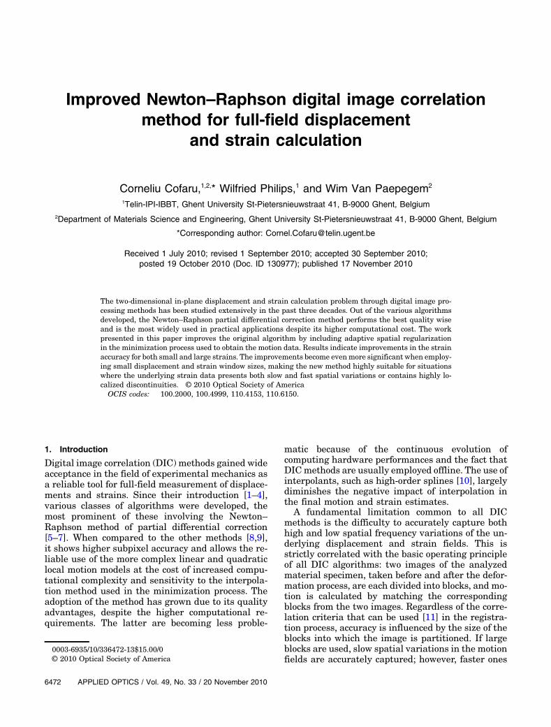
Fig. 1. Geman–McClure robust function (left) and its first derivative (right) for the shape parameter values σ ¼ 0:01, 0.1, 1.
20 November 2010 / Vol. 49, No. 33 / APPLIED OPTICS 6473

component, the influence of its neighbors is propor-tional to the first derivative ∂ρðr; σÞ=∂r of the robustfunction seen in Fig. 1, which decreases toward zerowhen jrijj > jσij. Furthermore, small σi values,equivalent to a large degree of smoothness in thearea around the displacement component currentlyestimated, lead to strong regularization using theclosest neighboring values. Alternatively, largervalues reflect strong changes in the displacementcomponent’s neighborhood—the influence that theneighbors exert on the component being limitedand more evenly distributed. In the currentimplementation,
σi ¼�7 ~σi; if i < 33 ~σi if i ≥ 3
ð6Þ
uses a higher multiplication factor of the local stan-dard deviation for the translational components P1and P2 because, in most cases, they represent the lar-gest component of the displacement vector and,hence, differences between neighbors are larger, ne-cessitating a more relaxed or flat robust influencefunction.
The minimization of Eq. (3) through the Newton–Raphson iterative method has the solution at the kthiteration of the following form:
PðkÞ − Pðk−1Þ ¼ −∇EðPðk−1ÞÞ∇∇EðPðk−1ÞÞ ; ð7Þ
where
∇EðPÞ ¼��
∂ED
∂P1þ λ ∂ES
∂P1
�� � �
�∂ED
∂P6þ λ ∂ES
∂P6
��; ð8Þ
∇∇EðPÞ ¼
26666664
�∂2ED
∂P21þ λ ∂2ES
∂P21
�� � �
�∂2ED∂P1∂P6
�
..
. . .. ..
.�∂2ED∂P6∂P1
�� � �
�∂2ED
∂P26þ λ ∂2ES
∂P26
�
37777775
ð9Þ
are the Jacobian and Hessian matrices, respectively,of the energy functional with the following regulari-zation term partial derivatives:
∂ES
∂Pi¼
Xj∈N8
i
2σiðPi − PjÞðσi þ ðPi − PjÞ2Þ2
; ð10Þ
∂2ES
∂P2i
¼Xj∈N8
i
2σ2i − 6σiðPi − PjÞ2ðσi þ ðPi − PjÞ2Þ3
; ð11Þ
respectively. Note that ∂2ES=∂P2i is only present on
the first diagonal of the Hessian because the second
partial derivatives of ES with respect to two differentdisplacement components are zero.
The method starts by dividing the reference imageinto blocks and finding the best match for each blockin the deformed image through cross-correlationcoefficient minimization. The resulting integer pixeldisplacements will represent the initial solution forthe Newton–Raphson minimization step of the meth-od. The latter updates at each iteration the entiremotion vector field, excluding the locations whereconvergence has already been reached. As conver-gence criterion, a difference smaller than 10−5 be-tween consecutive iterations for all displacementcomponents has been chosen. Once a motion vectorreached convergence, its six components will stopbeing updated; however, they will be used in subse-quent iterations in calculating the regularizationterms of their neighbors. If in three successive itera-tions the total number of motion vectors that reachedconvergence does not change, the algorithm stops. Toincrease the stability of the method, the first threeiterations are executed without taking into consid-eration the regularization terms.
3. Tests and Results
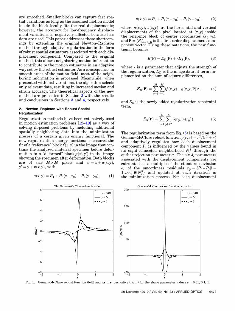
The evaluation of the new method consists of calcu-lating the displacements and strains in four experi-mental scenarios: two numerical simulations andtwo real mechanical experiments. Each scenario con-tains an image pair composed of a “reference” and a“deformed” image. The first two scenarios correspondto a “plate with hole under biaxial stress”model [20],with their deformed images numerically obtained bywarping a common reference speckle image usingknown displacements and radial basis function im-age interpolation [9]. In the third and fourth experi-mental scenarios, which represent real experiments,a plastic film specimen (25:3 mm in width, 250 mmin length, and 0:1 mm in thickness) with a lateral slitinto its right edge and an aluminum specimen(25:25 mm in width, 280 mm in length, and 2:95 mmin thickness) with two lateral slits on both edges un-dergo uniaxial load in a vertical upward direction. Allspeckle images were captured using a Pixelink PL-A782 camera at the maximum resolution of 2208 ×3000 pixels, out of which regions 1024 × 1024 pixelsin size were actively used in the tests. Through theexperimental setup, one pixel corresponds to 8:33 μmin the object plane for the first two experiments,11:92 μm in the third experiment, and 17 μm inthe fourth experiment. The camera was aligned per-pendicular to the specimen surface with a laser toeliminate out-of-plane displacement effects andcalibrated through the proprietary software to com-pensate for fixed-pattern noise, photo response non-uniformities, and lighting variations across thespecimen’s surface. The machine used to deformthe specimens in the last two experiments was a In-stron 8801 servo-hydraulic system. In Fig. 2, the tworeference images used in the first three scenariosare shown. The full camera frame as well as the
6474 APPLIED OPTICS / Vol. 49, No. 33 / 20 November 2010
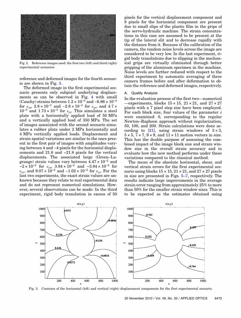
reference and deformed images for the fourth scenar-io are shown in Fig. 3.
The deformed image in the first experimental sce-nario presents only subpixel underlying displace-ments as can be observed in Fig. 4 with small(Cauchy) strains between 1:2 × 10⁻³ and −6:86 × 10−4
for εxx, 2:8 × 10⁻³ and −2:8 × 10⁻³ for εxy, and 4:7 ×10⁻³ and 1:73 × 10−5 for εyy. This simulates a steelplate with a horizontally applied load of 50 MPaand a vertically applied load of 350 MPa. The setof images associated with the second scenario simu-lates a rubber plate under 2 MPa horizontally and4 MPa vertically applied loads. Displacement andstrain spatial variations are similar to the ones pres-ent in the first pair of images with amplitudes vary-ing between 4 and −4 pixels for the horizontal displa-cements and 21.8 and −21:8 pixels for the verticaldisplacements. The associated large (Green–La-grange) strain values vary between 4:47 × 10−2 and−2 × 10⁻² for εxx, 3:84 × 10−2 and −3:84 × 10−2 forεxy, and 9:07 × 10−2 and −1:02 × 10−2 for εyy. For thelast two experiments, the exact strain values are un-known because they relate to real experimental dataand do not represent numerical simulations. How-ever, several observations can be made: In the thirdexperiment, rigid body translation in excess of 50
pixels for the vertical displacement component and8 pixels for the horizontal component are presentdue to small slips of the plastic film in the grips ofthe servo-hydraulic machine. The strain concentra-tions in this case are assumed to be present at thetip of the lateral slit and to decrease rapidly withthe distance from it. Because of the calibration of thecamera, the random noise levels across the image areconsidered to be very low. In the last experiment, ri-gid body translations due to slipping in the mechan-ical grips are virtually eliminated through bettergripping of the aluminum specimen in the machine.Noise levels are further reduced with respect to thethird experiment by automatic averaging of threecamera frames before and after deformation to ob-tain the reference and deformed images, respectively.
A. Quality Analysis
In the evaluation process of the first two—numerical—experiments, blocks 15 × 15, 21 × 21, and 27 × 27pixels with a 7 pixel step size have been employed.For each block size, four values of the parameter λwere examined: 0, corresponding to the regularNewton–Raphson approach without regularization,50, 100, and 200. Strain calculations were done ac-cording to [21], using strain windows of 3 × 3,5 × 5, 7 × 7, 9 × 9, and 11 × 11 motion vectors in size.This has the double purpose of assessing the com-bined impact of the image block size and strain win-dow size in the overall strain accuracy and toevaluate how the new method performs under thesevariations compared to the classical method.
The mean of the absolute horizontal, shear, andvertical strain errors for the first experimental sce-nario using blocks 15 × 15, 21 × 21, and 27 × 27 pixelsin size are presented in Figs. 5–7, respectively. Theresults indicate large improvements in the averagestrain error ranging from approximately 25% tomorethan 50% for the smaller strain window sizes. This isto be expected as the estimates obtained using
Fig. 2. Reference images used: the first two (left) and third (right)experimental scenarios.
Fig. 3. Contours of the horizontal (left) and vertical (right) displacement components for the first experimental scenario.
20 November 2010 / Vol. 49, No. 33 / APPLIED OPTICS 6475

regularization include neighboring spatial informa-tion and, thus, are more reliable than the nonregu-larized estimates. The proposed method producesthe minimum errors regardless of strain windowsand block sizes for the horizontal and verticalstrains. In the case of the shear strains, it performsbetter when using strain windows smaller than11 × 11. It is clearly noticeable that increases of thestrain window size, image block size, or both have alesser impact in the accuracy of the method whenusing regularization. This suggests increased practi-cal applicability of the proposed method in situationswhere these smaller sizes are required, such as low-resolution images or localized stress concentrations.The lower limit of the mean errors remains approxi-mately the same for all block sizes in the range of 150to 200 με.
The results from the second experiment, synthe-sized in Figs. 8–10, indicate that the introductionof spatial regularization improves the accuracy ofthe Newton–Raphson DIC method for larger strains,as well. The proposed method outperforms the clas-sical one at all strain window and image block sizes,providing also the absolute minimum errors. How-ever, it is interesting to notice that the minimum er-rors for all three strains were obtained using thesmallest image block size of 15 × 15 pixels and strainwindow sizes of either 7 × 7 or 9 × 9 motion vectors.The negative effect of larger strain windows isbecoming more evident as the image block size in-creases: for block sizes of 21 × 21 pixels and 27 ×
27 pixels, using a strain window of 7 × 7 motion vec-tors produces consistently better results than a 11 ×11 strain window. In the case of the vertical strains inFig. 10, strain windows sized at 5 × 5 produce smallererrors than the ones sized at 9 × 9 and 11 × 11. Be-sides the improvements brought by the proposedmethod, the results from the second experiment in-dicate that, unless the underlying strains that are tobe calculated present smooth variations, which inturn require solid prior knowledge about the experi-mental behavior of the analyzed mechanical speci-men, increasing the strain window sizes and imageblock sizes can lead to deterioration of the measuredstrain accuracy. It is, thus, preferable to use smallerblock sizes and strain window sizes to avoid over-smoothing the strain estimates with any addi-tional neighboring information pooled in an adaptivemanner.
The last two practical experiments are meant to bea only visual evaluation of the observations made forfirst two experimental scenarios because no numer-ical verification is possible. In the third experiment,two tests were done where the regularizationstrength parameter λ had the values of 0 and 1000.The value of λ is larger than in the previous tests sothat the stronger adaptive smoothing would compen-sate for any possible effects of camera noise presentin the images on the motion estimates. The block sizewas fixed at 27 × 27 pixels with a 7 pixel step. Largestrains are expected to be present at the tip of thecrack and its immediate vicinity with smaller and
Fig. 4. Mean absolute strain errors for the horizontal (left), shear (center), and vertical (right) small (Cauchy) strains as functions of thestrength regularization parameter λ and strain window size W using block sizes of 15 × 15 pixels.
6476 APPLIED OPTICS / Vol. 49, No. 33 / 20 November 2010
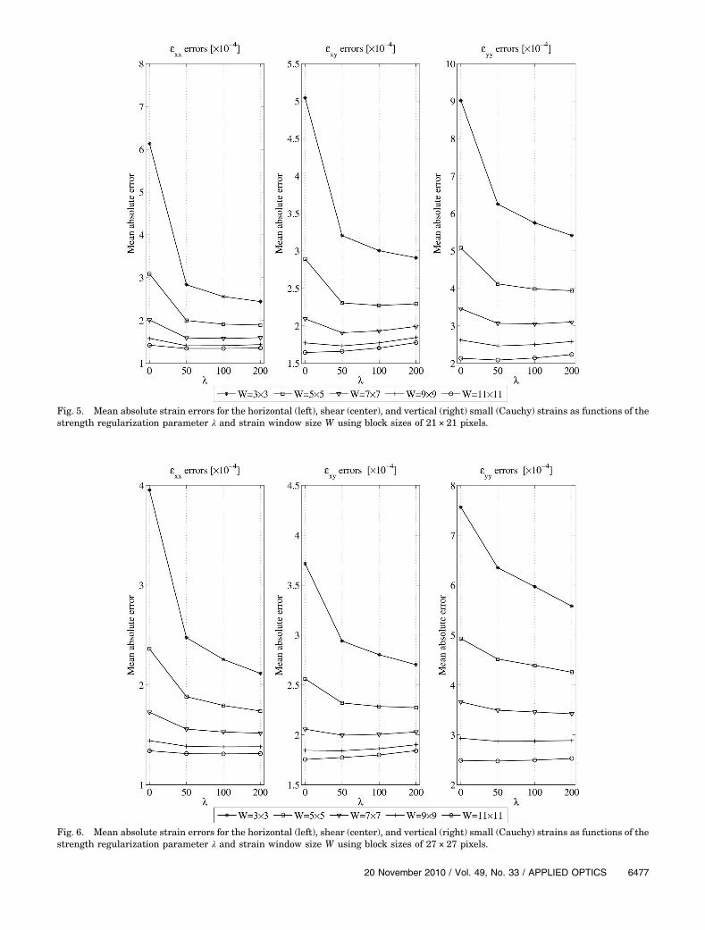
Fig. 5. Mean absolute strain errors for the horizontal (left), shear (center), and vertical (right) small (Cauchy) strains as functions of thestrength regularization parameter λ and strain window size W using block sizes of 21 × 21 pixels.
Fig. 6. Mean absolute strain errors for the horizontal (left), shear (center), and vertical (right) small (Cauchy) strains as functions of thestrength regularization parameter λ and strain window size W using block sizes of 27 × 27 pixels.
20 November 2010 / Vol. 49, No. 33 / APPLIED OPTICS 6477

Fig. 7. Mean absolute strain errors for the horizontal (left), shear (center), and vertical (right) large (Green–Lagrange) strains as func-tions of the strength regularization parameter λ and strain window size W using block sizes of 15 × 15 pixels.
Fig. 8. Mean absolute strain errors for the horizontal (left), shear (center), and vertical (right) large (Green–Lagrange) strains as func-tions of the strength regularization parameter λ and strain window size W using block sizes of 21 × 21 pixels.
6478 APPLIED OPTICS / Vol. 49, No. 33 / 20 November 2010
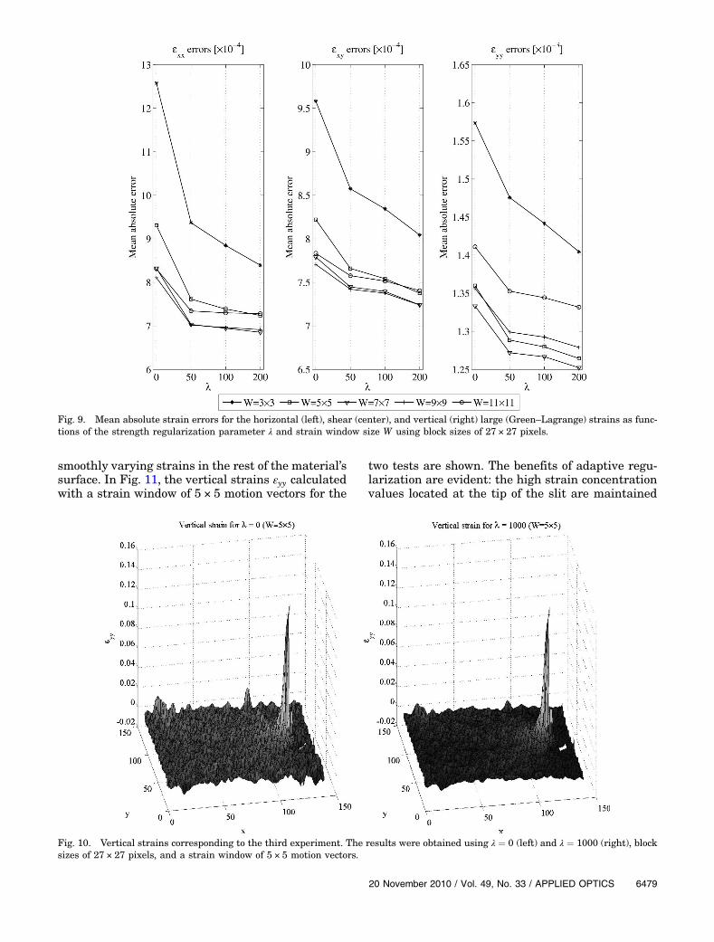
smoothly varying strains in the rest of the material’ssurface. In Fig. 11, the vertical strains εyy calculatedwith a strain window of 5 × 5 motion vectors for the
two tests are shown. The benefits of adaptive regu-larization are evident: the high strain concentrationvalues located at the tip of the slit are maintained
Fig. 9. Mean absolute strain errors for the horizontal (left), shear (center), and vertical (right) large (Green–Lagrange) strains as func-tions of the strength regularization parameter λ and strain window size W using block sizes of 27 × 27 pixels.
Fig. 10. Vertical strains corresponding to the third experiment. The results were obtained using λ ¼ 0 (left) and λ ¼ 1000 (right), blocksizes of 27 × 27 pixels, and a strain window of 5 × 5 motion vectors.
20 November 2010 / Vol. 49, No. 33 / APPLIED OPTICS 6479
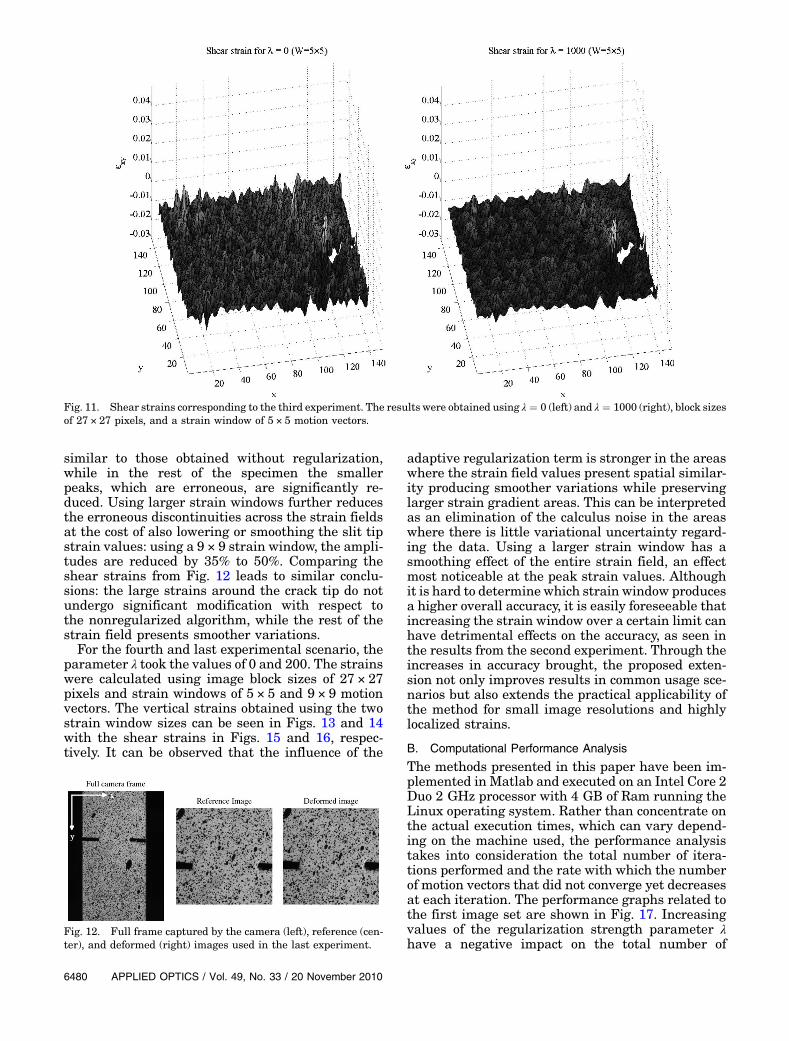
similar to those obtained without regularization,while in the rest of the specimen the smallerpeaks, which are erroneous, are significantly re-duced. Using larger strain windows further reducesthe erroneous discontinuities across the strain fieldsat the cost of also lowering or smoothing the slit tipstrain values: using a 9 × 9 strain window, the ampli-tudes are reduced by 35% to 50%. Comparing theshear strains from Fig. 12 leads to similar conclu-sions: the large strains around the crack tip do notundergo significant modification with respect tothe nonregularized algorithm, while the rest of thestrain field presents smoother variations.
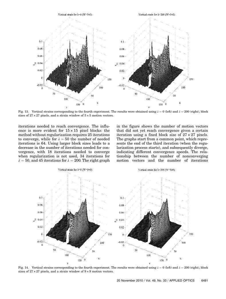
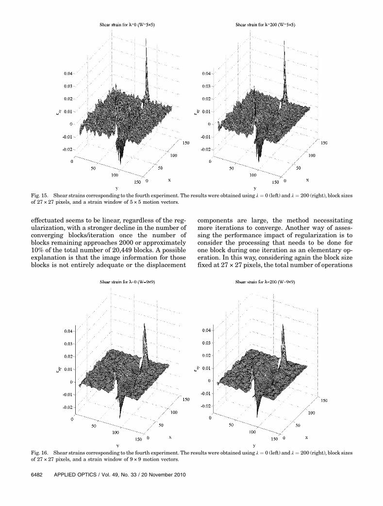
For the fourth and last experimental scenario, theparameter λ took the values of 0 and 200. The strainswere calculated using image block sizes of 27 × 27pixels and strain windows of 5 × 5 and 9 × 9 motionvectors. The vertical strains obtained using the twostrain window sizes can be seen in Figs. 13 and 14with the shear strains in Figs. 15 and 16, respec-tively. It can be observed that the influence of the
adaptive regularization term is stronger in the areaswhere the strain field values present spatial similar-ity producing smoother variations while preservinglarger strain gradient areas. This can be interpretedas an elimination of the calculus noise in the areaswhere there is little variational uncertainty regard-ing the data. Using a larger strain window has asmoothing effect of the entire strain field, an effectmost noticeable at the peak strain values. Althoughit is hard to determine which strain window producesa higher overall accuracy, it is easily foreseeable thatincreasing the strain window over a certain limit canhave detrimental effects on the accuracy, as seen inthe results from the second experiment. Through theincreases in accuracy brought, the proposed exten-sion not only improves results in common usage sce-narios but also extends the practical applicability ofthe method for small image resolutions and highlylocalized strains.
B. Computational Performance Analysis
The methods presented in this paper have been im-plemented in Matlab and executed on an Intel Core 2Duo 2 GHz processor with 4 GB of Ram running theLinux operating system. Rather than concentrate onthe actual execution times, which can vary depend-ing on the machine used, the performance analysistakes into consideration the total number of itera-tions performed and the rate with which the numberof motion vectors that did not converge yet decreasesat each iteration. The performance graphs related tothe first image set are shown in Fig. 17. Increasingvalues of the regularization strength parameter λhave a negative impact on the total number of
Fig. 11. Shear strains corresponding to the third experiment. The results were obtained using λ ¼ 0 (left) and λ ¼ 1000 (right), block sizesof 27 × 27 pixels, and a strain window of 5 × 5 motion vectors.
Fig. 12. Full frame captured by the camera (left), reference (cen-ter), and deformed (right) images used in the last experiment.
6480 APPLIED OPTICS / Vol. 49, No. 33 / 20 November 2010
iterations needed to reach convergence. The influ-ence is more evident for 15 × 15 pixel blocks: themethod without regularization requires 25 iterationsto converge, while for λ ¼ 50 the number of needediterations is 64. Using larger block sizes leads to adecrease in the number of iterations needed for con-vergence, with 18 iterations needed to convergewhen regularization is not used, 34 iterations forλ ¼ 50, and 45 iterations for λ ¼ 200. The right graph
in the figure shows the number of motion vectorsthat did not yet reach convergence given a certainiteration using a fixed block size of 27 × 27 pixels.The graphs start from a common point, which repre-sents the end of the third iteration (when the regu-larization process starts), and subsequently diverge,indicating different convergence speeds. The rela-tionship between the number of nonconvergingmotion vectors and the number of iterations
Fig. 13. Vertical strains corresponding to the fourth experiment. The results were obtained using λ ¼ 0 (left) and λ ¼ 200 (right), blocksizes of 27 × 27 pixels, and a strain window of 5 × 5 motion vectors.
Fig. 14. Vertical strains corresponding to the fourth experiment. The results were obtained using λ ¼ 0 (left) and λ ¼ 200 (right), blocksizes of 27 × 27 pixels, and a strain window of 9 × 9 motion vectors.
20 November 2010 / Vol. 49, No. 33 / APPLIED OPTICS 6481
effectuated seems to be linear, regardless of the reg-ularization, with a stronger decline in the number ofconverging blocks/iteration once the number ofblocks remaining approaches 2000 or approximately10% of the total number of 20,449 blocks. A possibleexplanation is that the image information for thoseblocks is not entirely adequate or the displacement
components are large, the method necessitatingmore iterations to converge. Another way of asses-sing the performance impact of regularization is toconsider the processing that needs to be done forone block during one iteration as an elementary op-eration. In this way, considering again the block sizefixed at 27 × 27 pixels, the total number of operations
Fig. 15. Shear strains corresponding to the fourth experiment. The results were obtained using λ ¼ 0 (left) and λ ¼ 200 (right), block sizesof 27 × 27 pixels, and a strain window of 5 × 5 motion vectors.
Fig. 16. Shear strains corresponding to the fourth experiment. The results were obtained using λ ¼ 0 (left) and λ ¼ 200 (right), block sizesof 27 × 27 pixels, and a strain window of 9 × 9 motion vectors.
6482 APPLIED OPTICS / Vol. 49, No. 33 / 20 November 2010

needed to reach convergence for λ ¼ 0 is 90,092, forλ ¼ 50 is 193,141, for λ ¼ 100 is 234,378, and for λ ¼200 is 281,746. A clear conclusion is that the speeddoes not decrease linearly with λ but rather tendsto saturate. The performance observations remainoverall unchanged for the second set of images,where larger strains are present; the only differenceis an increased overhead needed to calculate the lar-ger integer displacements.
4. Conclusion
In this paper, an extension of the Newton–Raphsonpartial differential correction DIC method throughthe addition of adaptive spatial regularization hasbeen presented and its accuracy and performance im-pact investigated. The regularization terms based onthe Geman–McClure robust function adaptivelyintegrate neighboring information motion into themotion estimates and are recalculated at each itera-tion to adjust the neighbor influence according to thelocal spatial smoothness in each displacement com-ponent field. Results indicate accuracy improve-ments consisting in mean errors up to 50% smallercompared to the nonregularized method for bothsmall and large strains. The quality advantages ofthe regularized method for smaller image blocksand strain windows are strongly desired becausetheir smaller sizes increase the locality of the avail-able deformation information. The inclusion of theregularization term increases the computational cost
of the method, which in turn is influenced by thestrength of the regularization and sizes of the imageblocks used in the motion estimation process. De-spite the computational costs, the quality advan-tages brought by the proposed method make it aviable alternative to existing DIC methods.
The authors acknowledge the Interuniversity At-traction Poles Program (IUAP-VI) of the Belgian Fed-eral Science Policy.
References1. W. H. Peters and W. F. Ranson, “Digital imaging techniques in
experimental stress-analysis,” Opt. Eng. 21, 427–431 (1982).2. M. A. Sutton, W. J. Wolters, W. H. Peters, W. F. Ranson, and S.
R. McNeill, “Determination of displacements using an im-proved digital correlation method,” Image Vis. Comput. 1,133–139 (1983).
3. C.-H. Teng, S.-H. Lai, Y.-S. Chen, and W.-H. Hsu, “Accurateoptical flow computation under non-uniform brightnessvariations,” Comput. Vis. Image Underst. 97, 315–346(2005).
4. W. H. Peters, W. F. Ranson, M. A. Sutton, T. C. Chu, and J.Anderson, “Applications of digital correlation methods to rigidbody mechanics,” Opt. Eng. 22, 738–742 (1983).
5. T. C. Chu, W. F. Ranson, M. A. Sutton, and W. H. Peters, “Ap-plications of digital-image-correlation techniques to experi-mental mechanics,” Exp. Mech. 25, 232–244 (1985).
6. H. A. Bruck, S. R. McNeill, M. A. Sutton, and W. H. Peters,“Digital image correlation using Newton-Raphson methodof partial differential correction,” Exp. Mech. 29, 261–267(1989).
Fig. 17. Number of iterations as a function of the strength regularization parameter λ for different block sizes (left) and the number ofmotion vectors that did not yet converge for a fixed block size of 27 × 27 pixels for different λ values (right).
20 November 2010 / Vol. 49, No. 33 / APPLIED OPTICS 6483
7. G. Vendroux and W. G. Knauss, “Submicron deformation fieldmeasurements: part 2. Improved digital image correlation,”Exp. Mech. 38, 86–92 (1998).
8. H. Lu and P. D. Cary, “Deformation measurements by digitalimage correlation: implementation of a second-order displace-ment gradient,” Exp. Mech. 40, 393–400 (2000).
9. B. Pan, H.-M. Xie, B.-Q. Xu, and F.-L. Dai, “Performance ofsub-pixel registration algorithms in digital image correlation,”Meas. Sci. Technol. 17, 1615–1621 (2006).
10. C. Cofaru, W. Philips, and W. Van Paepegem, “Evaluation ofdigital image correlation techniques using realistic groundtruth speckle images,” Meas. Sci. Technol. 21, 055102(2010).
11. M. A. Sutton, J.-J. Orteu, and H. W. Schreier, Image Correla-tion for Shape, Motion and Deformation Measurements(Springer, 2009).
12. B. Pan, K-M. Qian, H-M. Xie, and A. Asundi, “Two-dimensional digital image correlation for in-plane displace-ment and strain measurement: a review,” Meas. Sci. Technol.20, 062001 (2009).
13. M. Ye, R. M. Haralick, and L. G. Shapiro, “Estimating piece-wise-smooth optical flow with global matching and graduatedoptimization,” IEEE Trans. Pattern Anal. Mach. Intell. 25,1625–1630 (2003).
14. G. Le Besnerais and F. Champagnat, “B-spline image modelfor energy minimization-based optical flow estimation,” IEEETrans. Image Process. 15, 3201–3206 (2006).
15. J.-D. Kim and J. Kim, “Effective nonlinear approach for opticalflow estimation,” Signal Process. 81, 2249–2252 (2001).
16. M. J. Black and P. Anandan, “The robust estimation of multi-ple motions: parametric and piecewise-smooth flow fields,”Comput. Vis. Image Underst. 63, 75–104 (1996).
17. Y.-H. Kim, A. M. Martìnez, and A. C. Kak, “Robust motion es-timation under varying illumination,” Image Vis. Comput. 23,365–375 (2005).
18. J. Weickert and C. Schnorr, “Variational optic flow computa-tion with a spatio-temporal smoothness constraint,” J. Math.Imaging Vision 14, 245–255 (2001).
19. A. Bruhn, J. Weickert, and C. Schnorr, “Lucas/Kanade meetsHorn/Schunck: combining local and global optic flow meth-ods,” Int. J. Comput. Vis. 61, 1 (2005).
20. J. F. Cárdenas-García and J. J. E. Verhaegh, “Catalogue ofMoiré fringes for a bi-axially-loaded infinite plate with a hole,”Mech. Res. Commun. 26, 641–648 (1999).
21. B. Pan, A. Asundi, H.-M. Xie, and J. X. Gao, “Digital imagecorrelation using iterative least squares and pointwise leastsquares for displacement field and strain field measure-ments,” Opt. Lasers Eng. 47, 865–874 (2009).
6484 APPLIED OPTICS / Vol. 49, No. 33 / 20 November 2010