improved magnetic circuit analysis of a laminated
TRANSCRIPT

1
Improved magnetic circuit analysis of a laminated magnetorheological
elastomer devices featuring both permanent magnets and electromagnets
Shaoqi Li1, Peter A. Watterson2, Yancheng Li1,3*, Quan Wen4, Jianchun Li1
1. School of Civil and Environmental Engineering, Faculty of Engineering and Information Technology,
University of Technology Sydney, Ultimo, NSW 2007, Australia
2. School of Electrical and Data Engineering, Faculty of Engineering and Information Technology, University
of Technology Sydney, Ultimo, NSW 2007, Australia
3. School of Civil Engineering, Nanjing Tech University, Nanjing 211816, China
4. School of Mechanical Engineering, Nanjing University of Science and Technology, Nanjing 210094, China
Email: [email protected]; [email protected];
Abstract
As an essential and critical step, magnetic circuit modelling is usually implemented in the design
of efficient and compact magnetorheological (MR) devices, such as MR dampers and MR
elastomer isolators. Conventional magnetic circuit analysis simplifies the analysis by ignoring the
magnetic flux leakage and magnetic fringing effect. These assumptions are sufficiently accurate in
dealing with less complicated designs, featuring short magnetic path lengths such as in an MR
damper. However, when dealing with MR elastomer devices, such simplification in magnetic
circuit analysis results in inaccuracy of dimensioning and performance estimation of the devices
due to their sophisticated design and complex magnetic paths. Modelling permanent magnets also
imposes challenges in the magnetic circuit analysis. This work proposes an improved approach to
include magnetic flux fringing effect in magnetic circuit analysis for MR elastomer devices. An
MRE-based isolator containing multiple MRE layers and both a permanent magnet and an exciting
coil was designed and built as a case study. The results of the proposed method are compared to

2
those of conventional magnetic circuit modelling, finite element analysis and experimental
measurements to demonstrate the effectiveness of the proposed approach.
Keywords
Magnetorheological elastomer; magnetic circuit modelling; flux fringing effect; permanent magnet
1. Introduction
Dispersing ferromagnetic particles in elastomeric solids obtains a class of smart material normally
termed magnetorheological elastomer (MRE) [1]. It exhibits a unique and useful phenomenon
which is tunable material properties, i.e., stiffness and damping, upon the application of external
magnetic field. Benefiting from this phenomenon, successfully applications have been reported in
the fields of civil engineering [2,3] and mechanical engineering [4,5] for structural control and
vibration reduction purposes; and, recently, its potentials have been further extended to developing
sensors, robots and wearables [6-9].
One of the major branches of MRE-based application is isolators which can achieve adaptive
isolation performance against different types of seismic conditions due to its tunable stiffness and
damping [10]. Drawing on the design of commercial laminated rubber bearings, the multi-layer
configuration is normally adopted in MRE isolators due to its excellence in carrying vertical
loading with the minimal bulging effect in the elastomer layers. Li et al. developed the first
adaptive base isolator with 47 layers of MRE [11]. Based on this configuration, Li et al. further
improved the adaptive range of base isolators by developing a highly adjustable base isolator with
1630% increase of lateral stiffness [12]. Harnessing the benefits of this highly adjustable isolator,
Gu et al. constructed a real-time controlled smart seismic isolation system and conducted a series
of concept-proof experiments with sound outcomes [13]. Following these successful developments,
3
numerous researches on the multi-layer structured MRE isolators have been carried out. Xing et
al. developed a novel base isolator with 20 layers of MRE [14]. Although these applications all
achieve sound vibration mitigation performances, solely relying on electromagnet coils to provide
magnetic field for the devices brings significant thermal and energy consumption issues [15]. In
the applications for base isolators or bridge bearings where higher lateral stiffness is required to
resist small disturbances like wind load and building live load in the majority of the service life,
the coils in the device should be powered continuously [16]. Addressing these issues, the
innovation of utilizing both electromagnet coils and permanent magnets (PM) has been proposed.
The introduction of permanent magnets (PMs) provides MRE devices with a “bias” magnetic field
present when the electric current is zero, which can reduce energy consumption. A positive or
negative electric current can be applied to increase or decrease the magnetic field and tailor the
device properties. For example, hybrid magnets laminated MRE adaptive isolators designed by
Yang et al. [16] and Sun et al. [17] realized stiffness softening capability, maintaining stability
without power during normal service life, and achieving effective base isolation during seismic
events.
However, implementing the multi-layered structure and PM both adds difficulty and challenge to
the design of device configuration and analysis of electromagnetic performance. For multi-layered
structure, steel sheets with high relative permeability, which is normally around 5000, are chosen
to bond with MRE layers to give a higher conductivity for magnetic field. However, the relative
permeability of MRE is usually as low as 1 to 7 [18]. Laminating these two types of material may
result in magnetic fluxes leaking out from high permeability layers, forming unpredicted flux paths
and irregular flux density distributions in the multi-layer structure. As for using PM, the
complexities lie in the inhomogeneous magnetic field distribution on the PM surfaces and the

4
prevention of irreversible demagnetization. Considering the strong magnetic field dependence of
MR materials, revealing the magnetic field distribution inside of the laminated MRE devices
featuring hybrid magnets is critical and mandatory to achieve cost-effective and reliable designs.
However, this cannot be achieved by experimental methods, since current available magnetic field
sensors are not capable of detecting the field distribution inside of a cured laminated structure
without any structural modifications on the device. And opening slots on the laminated structure
to accommodate the sensor will cause the detour of magnetic flux path and unreliable
measurements.
Numerically, standard practice is to undertake the design using finite element software, such as
ANSYS Maxwell or COMSOL Multiphysics. However, the construction of FEA models requires
comprehensive details of the device which are commonly not available at the initial design stage.
To obtain an optimal design of an MR device often involves numerous rounds of trial-and-error.
Another analysis approach in developing magnetorheological (MR) devices, namely magnetic
circuit modelling (MCM), produces equational presentations of the relationships between the
device performance and variables such as the magnetic field strength, material properties and
dimensions of the components. MCM allows theoretical, quantitative analysis and optimization
focusing on predominant design parameters without involving much effort in modifying the
geometry of the design and physical properties of the used materials in the first place. MCM has
been successfully used in developing, analyzing and optimizing MR fluid dampers [19-25], MR
fluid actuators [26-28] and MR fluid valves [29-32].
However, MR fluid devices and MRE devices should be treated separately when considering
MCM as a design technique. For MR fluid devices, large damping force can be realized by
controlling the flow of fluid through narrow channels permeated by the controllable magnetic field.

5
Therefore, the magnetic path of MR fluid devices is normally simple and of small length-scale.
Simple device configurations result in homogeneous magnetic field distributions in the MR fluid.
In such configurations, the standard MCM assumptions of no branched magnetic flux paths and
no flux fringing are accurate, and thus the conventional MCM method is viable. However, making
these assumptions can dramatically degrade the accuracy and reliability in designing MRE devices
especially multilayer MRE devices which include larger length-scale and branched magnetic flux
paths. In addition, unlike the sealed structure of MR fluid devices, air gaps and free spaces are
usually allocated in MRE devices to avoid friction or collision of moveable parts during shear
movements. The existence of air gaps introduces considerable flux fringing effect and imposes
design challenges as a consequence. Furthermore, the multilayer structure of MRE devices results
in inhomogeneous field distribution in the device. Wang et al. [33] suggested a design methodology
incorporating finite element analysis (FEA) to design an MRE-based isolator featuring a ten-
layered laminated conical-shaped core. The magnetic field analysis showed that the average
magnetic flux density varied over a factor 2 between the top and middle layers of MRE. Xing et
al. [34] also pointed out substantial differences of magnetic flux density at different locations in
the laminated structure of an MRE bearing. The inhomogeneous distribution of magnetic flux
density among MRE layers triggers different MR effects and causes discrepancies of mechanical
performance of the devices. These phenomena suggest that the flux leakage and branched flux
paths should be included in MCM for multilayer MRE devices. Though structural complexities of
MRE devices imply challenges in implementing the MCM method, some pilot investigations have
been conducted. Zhou [35] and Zhou et al. [36] iterated equational relationships between magnetic
flux densities and device specifications of MRE shear testing rigs through MCM. Böse et al. [37]
adopted MCM for evaluating the performance of an MRE valve. Yang et al. [38] computed the

6
magnetic field distribution of a shear-compression mixed mode MRE isolator by MCM and
obtained close results to FEA. However, these existing MCM implementations for MRE devices
made the same no flux-fringing assumptions as adopted for MR fluid devices and no multilayer
MRE structures with a hybrid magnets configuration were investigated. Hence, practical guidance
on developing MCM for hybrid magnets multi-layer MRE devices is of urgent demand.
In this work, an improved MCM approach to accurately analyze hybrid magnetic circuits involving
laminated MRE materials is proposed. The new approach considers the magnetic flux fringing
effect and branched magnetic flux paths and is therefore able to produce effective and efficient
estimation of the magnetic field in the device with complicated structure. With revealing the
equations of the relationships between device design parameters and magnetic flux density values,
this approach also greatly avails the optimization process at the device design stage. A laminated
MRE device featuring hybrid magnets was designed and manufactured as a benchmark case study.
The accuracy of the proposed approach is validated via FEA results and experimental
measurements.
2. Description of the benchmark device
Figure 1 shows the schematic diagram and a half of the section view with the illustration of the
main flux paths of the proposed hybrid MRE isolator. The main body of the device adopts the
proven design by Li et al. [11, 12] which is able to produce a good level of magnetic field across
the MRE layers. That design is modified by the inclusion of a PM of thickness 5 mm and diameter
100 mm, sandwiched in the middle of the steel laminated MRE core. 9 layers of MRE and 9 layers
of steel are laminated alternatively and bonded on both sides of the PM. The first layer attached to
each of the two pole faces of the PM is steel. All steel and MRE layers are 1 mm thick. An air gap

7
of thickness 5 mm between the top plate and the yoke allows horizontal movement. Steel
cylindrical blocks of height 37 mm were positioned between the MRE core and the top and bottom
plates. Ten small coils, each having 350 turns, are stacked together and connected in parallel to a
power supply. Detailed specifications for each component of the isolator are listed in Table 1.
Two magnetic field sources are specified in the device, namely the PM and the coil. When no
current is applied to the coil, magnetic field is sourced from the PM. In this way, the MRE layers
will maintain a higher stiffness without requiring any external electric power supplied to the device.
The magnetic flux generated by the PM travels through the laminated MRE core, steel parts and
the air gap, forming the major magnetic flux travel path. The intended current direction in the coil
is such as to create magnetic flux opposing the magnetic flux generated by the PM hence reducing
the magnetic flux densities in the MRE layers. The stiffness of the MRE material therefore
decreases. Hence, softening and adaptability can be achieved by applying and varying the current
supplied to the coil.
Figure 1. Overview and schematic (not to scale) of the proposed isolator. The fluxes generated by
the coil and the PM are represented by the blue dashed line and the solid red line respectively.

8
Table 1. Specifications of the components of the isolator
Material Quantity Axial Height (mm) Diameter (mm)
Steel Block Steel 1008 2 37 100
Steel Plate Steel 1008 2 10 250
Yoke Steel 1008 1 110 180 (inner);
220 (outer)
Steel Sheet Steel 1008 18 1 100
MRE Sheet MRE 18 1 100
PM N40 NdFeB 1 5 100
3. Conventional MCM analysis
(a) Without current applied to coil (b) With current applied to coil
Figure 2. Magnetic circuit models without considering magnetic fringing
On the assumption that no fringing is considered, conventional MCM for the proposed isolator can
be depicted as Figure 2. By assuming all components of the isolator are in series connection, the
same flux travels through every part and is equivalent to the total flux Ø. The hybrid magnetic
circuit, Figure 2(b), features the superposition of a magnetomotive force (MMF) from the PM,
denoted FPM, and an MMF from the coil, denoted Fcoil, which operates in the opposite direction to
that of FPM. MMF values for PM and coil can be calculated by equation (1):
𝐹PM = 𝐻𝑐𝑙PM
𝐹coil = 𝑁𝑖 (1)

9
where Hc is the coercivity of the PM, 𝑙PM is the magnet thickness, N is the total number of turns
of the coil, and i is the current in each turn. Since all components are in series, the total circuit
reluctance is the sum of the reluctances for each type of material, RMRE, Rsteel, Rairgap, and RPM,
which are given by equation (2):
𝑅MRE = 𝑛𝑙MRE/(𝜇MRE𝐴MRE)
𝑅airgap = 𝑙airgap/ (𝜇air𝐴airgap)
𝑅PM = 𝑙PM/(𝜇PM𝐴PM)
𝑅steel = 𝑙yoke/(𝜇yoke𝐴yoke) + 2𝑙plate/(𝜇plate𝐴plate) +
2𝑙block/ (𝜇block𝐴block) + 𝑛𝑙steel sheet/(𝜇steel sheet𝐴steel sheet),
(2)
where n is the total number of MRE layers, also equal the total number of steel sheet layers, l is
the flux path length through each element, A is the flux cross-sectional area of each element, and
𝜇 =𝐵
𝐻 is the element permeability, for H the magnetic field and B the magnetic flux density. For
air, 𝜇 = 𝜇0. The N40 NdFeB magnet was assumed to have linear B-H curve in the second quadrant
with remanence 𝐵rem = 1.25 T and coercivity 𝐻c = 9.5 × 10⁵Am−1. The magnet is modelled as
a cylindrical surface current of density 𝐻c around the magnet perimeter with the interior of the
magnet treated as having permeability 𝜇PM =𝐵rem
𝐻c= 1.3158 × 10⁻⁶Hm−1 = 1.047𝜇0 . The
relationship between B and H for steel and MRE are presented in Figure 3 and symbolically
expressed in equation (3):
𝐻steel = 𝑓steel(𝐵steel)
𝐻MRE = 𝑓MRE(𝐵MRE) (3)

10
Figure 3. B-H curves for steel and MRE
B in each element is related to the flux and the element cross-sectional area by:
∅ = 𝐵𝐴. (4)
For the top and bottom plates of this circuit, A varies with radius. For the plate thickness chosen,
the largest cylindrical cross-sectional area was smaller than the planar areas where the flux entered
and exited the plate. The cylindrical cross-sectional area at the average of the inner yoke radius
and the block outer radius was used. As a check against saturation, the MCM was repeated using
the smallest area, at the block outer radius, and the results were found to change insignificantly.
The calculations of the A and l values are specified in Appendix A.
The mathematical expressions of the magnetic circuit models constructed in Figure 2(a)
and (b) can be expressed as equation (5) and (6), respectively:
𝐹pm = 𝐻𝑐𝑙PM = ∑ 𝑓steel (∅
𝐴𝑖) 𝑙𝑖
+ ∑ 𝑓MRE (∅
𝐴𝑖) 𝑙𝑖
+∅𝑙airgap
𝜇air𝐴airgap+
∅𝑙PM
𝜇PM𝐴PM (5)
0
0.5
1
1.5
2
0 200 400 600 800
B (
T)
H (kA/m)
MRE
0
0.5
1
1.5
2
0 6 12 18
B (
T)
H (kA/m)
Steel 1008

11
𝐹pm − 𝐹coil = 𝐻𝑐𝑙PM − 𝑁𝑖
= ∑ 𝑓steel (∅
𝐴𝑖) 𝑙𝑖
+ ∑ 𝑓MRE (∅
𝐴𝑖) 𝑙𝑖
+∅𝑙air
𝜇air𝐴airgap+
∅𝑙PM
𝜇PM𝐴PM
(6)
By substituting specifications and dimensions of each part of the isolator, the main flux Ø is
obtained and can be converted to magnetic flux densities distributed in each element through
equation (4). Summarising Appendix A, Table 2 lists the MCM parameters of the isolator elements.
Table 2 Conventional MCM parameters for the MRE isolator
n l (mm) A (mm2)
Steel Block 2 37 7853.98
Steel Plate 2 110 4398.23
Yoke 1 110 12566.37
Steel Sheet 18 1 7853.98
MRE Sheet 18 1 7853.98
Air Gap 1 5 12566.37
PM 1 5 7853.98
Results from the conventional MCM for current applied to each small coil ranging from 0 A to
1.357 A are presented in Figure 4. The magnetic flux densities in all MRE layers is seen to decrease
from 0.49 T to 0 T when the applied i increased from 0 A to 1.357 A. For the total number of turns
N = 3500, 1.357 A current gives 4750 Aturns MMF of the ten coils (where Aturns is the product
of the current times the number of turns) which is equal to the MMF of the PM, 𝐻c𝑙PM, therefore,
at this current, the magnetic field of the PM is cancelled out theoretically by the field generated by
the coil. Although this method provides rapid solutions for estimating electromagnetic properties,
the assumptions include ignoring the flux leakage and fringing effects; hence the amount of flux
travelling throughout the entire circuit model is constant and flux density values are identical for

12
components sharing the same A value. Hence, for the laminated core area, flux density values in
MRE sheets and steel sheets are the same, which is an inaccurate description of the magnetic flux
density distribution for devices featuring laminated cores.
Figure 4. Magnetic flux density in MRE from MCM without considering fringing effect
4. FEA results
An axisymmetric finite element model of the prototype hybrid magnetic isolator was constructed
and analysed through ANSYS Electronic Desktop. The software solved for the azimuthal
component of the magnetic vector potential. Isotropic permeability was assumed for all materials.
The N40 NdFeB magnet was assumed to have linear B-H curve in the second quadrant with
remanence 𝐵rem = 1.25 T and coercivity 𝐻𝑐 = 9.5 × 10⁵Am−1. Solutions for current applied to
each small coil, i, ranging from 0 A up to 1.357 A, at values corresponding to current MMF values
0 Aturns, 1000 Aturns, 2000 Aturns, 3000 Aturns, 4000 Aturns and 4750 Aturns, were computed
in Figure 5. Due to the axial symmetry of the device, ½-axisymmetric presentations of the magnetic

13
flux density (B) plots are shown. Figure 5 (a) shows the B plot for 0 A in the coil, i.e. with the PM
as the magnetic source. Magnetic flux fringing can be clearly observed at the air gap and around
the laminated core area. Figure 5 (b)-(f) show the results as the i increases up to 1.357 A.
(a) i = 0 A (b) i = 0.286 A
(c) i = 0.571 A (d) i = 0.857 A
14
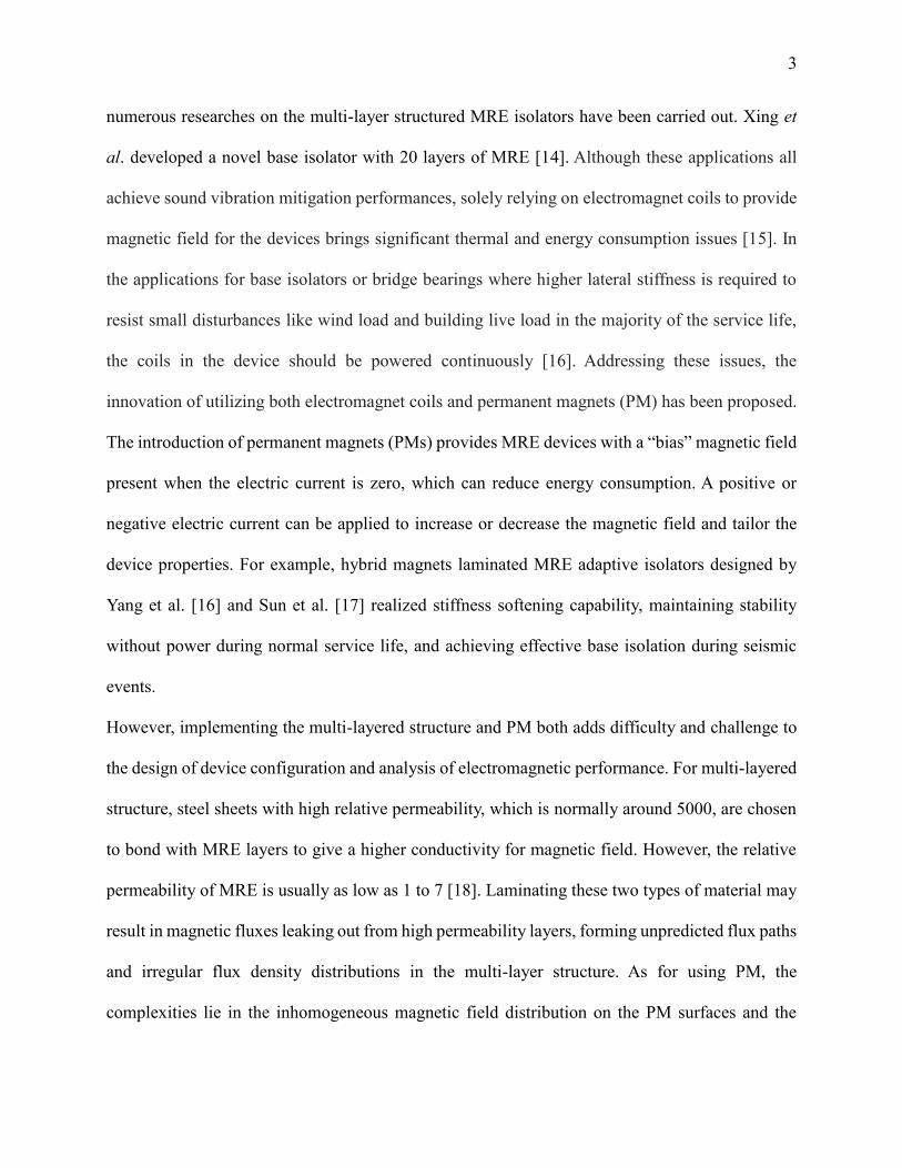
(e) i = 1.143 A (f) i = 1.357 A
Figure 5. Magnetic flux density plot from FEA
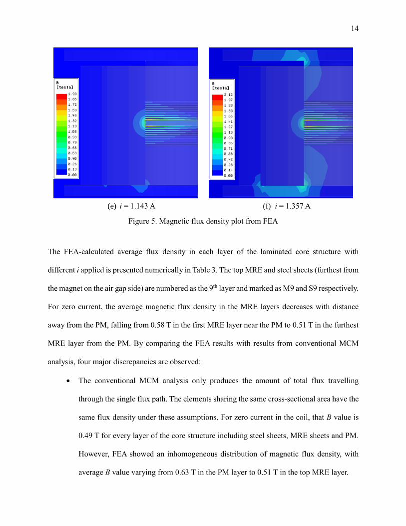
The FEA-calculated average flux density in each layer of the laminated core structure with
different i applied is presented numerically in Table 3. The top MRE and steel sheets (furthest from
the magnet on the air gap side) are numbered as the 9th layer and marked as M9 and S9 respectively.
For zero current, the average magnetic flux density in the MRE layers decreases with distance
away from the PM, falling from 0.58 T in the first MRE layer near the PM to 0.51 T in the furthest
MRE layer from the PM. By comparing the FEA results with results from conventional MCM
analysis, four major discrepancies are observed:
The conventional MCM analysis only produces the amount of total flux travelling
through the single flux path. The elements sharing the same cross-sectional area have the
same flux density under these assumptions. For zero current in the coil, that B value is
0.49 T for every layer of the core structure including steel sheets, MRE sheets and PM.
However, FEA showed an inhomogeneous distribution of magnetic flux density, with
average B value varying from 0.63 T in the PM layer to 0.51 T in the top MRE layer.

15
The conventional MCM analysis cannot capture the vector property of magnetic flux
density. For example, in FEA, high magnetic flux densities were observed in the 1st and
2nd steel layers, namely 1.04 T and 0.70 T respectively. These values are unusual
according to the conventional MCM since the flux density produced within the PM is
0.63 T. However, the explanation lies in the vector property of magnetic field: besides
the longitudinal magnetic flux density component, there are the fringing magnetic fluxes
leaking along the radial direction of the steel layers and the 1 mm thickness gives a
narrow magnetic flux path. As a result, the small amount of fringing flux produces a high
radial flux density component which contributes to produce high total magnetic flux
density values in the steel layers. Within each MRE sheet, the flux density is nearly all
longitudinal and is close to uniform in amplitude across the layer. However, in the steel
sheets, the high permeability allows the flux a low reluctance radial path to the outer
perimeter of the sheet and, especially for the 1st and 2nd steel sheets, a short leakage flux
path to the other side of the PM.
When the applied current in the coil increases to the equivalent amount of 𝐹PM, the coil
offsets the net magnetic flux density to 0 T everywhere in the conventional MCM.
However, the FEA shows that in fact a flux density of 0.11 T remains in the PM.
Associated with the magnetic fringing flux, the average flux density values in the 1st and
2nd steel layers still remained as high as for zero current in the coil.
Flux fringing can also be observed at the air gap between the top plate and the yoke. In
conventional MCM, the air gap is represented by a cylindrical annulus with the same
inner and outer diametric as the yoke. However, as shown in the FEA magnetic flux
density plot, instead of travelling straight across the modelled air gap, the flux fringes to
16
a larger area. Referring to equation (2), this will result in an error in estimating the
reluctance of the air gap and therefore output an unreliable MCM result.
Table 3 Average flux densities (T) in each layer of the core structure
0 A 0.286 A 0.571 A 0.857 A 1.143 A 1.357 A
M9 0.51 0.40 0.28 0.14 0.00 0.10
S9 0.51 0.40 0.29 0.17 0.10 0.15
M8 0.51 0.40 0.28 0.15 0.01 0.09
S8 0.52 0.41 0.30 0.19 0.12 0.17
M7 0.51 0.40 0.28 0.15 0.02 0.09
S7 0.52 0.42 0.31 0.21 0.15 0.18
M6 0.52 0.41 0.29 0.16 0.03 0.08
S6 0.53 0.43 0.33 0.23 0.18 0.20
M5 0.52 0.42 0.30 0.17 0.04 0.06
S5 0.55 0.45 0.35 0.27 0.22 0.24
M4 0.53 0.43 0.31 0.18 0.05 0.05
S4 0.57 0.48 0.39 0.31 0.28 0.30
M3 0.54 0.44 0.32 0.20 0.07 0.04
S3 0.60 0.53 0.45 0.41 0.40 0.42
M2 0.56 0.45 0.34 0.21 0.09 0.02
S2 0.70 0.66 0.62 0.67 0.71 0.75
M2 0.58 0.47 0.36 0.24 0.12 0.04
S1 1.04 1.02 0.99 1.03 1.02 1.04
PM 0.63 0.54 0.43 0.32 0.20 0.11
5. The proposed MCM analysis
The discrepancies above originate from the overly simplified assumptions adopted, such as single
magnetic path with no fringing, simple air gap path, etc. A modified approach should be
constructed in order to obtain more accurate magnetic field distributions. In the following, several
modifications are applied in the proposed MCM, including modelling flux fringing in the air gap
and around the magnet.
17
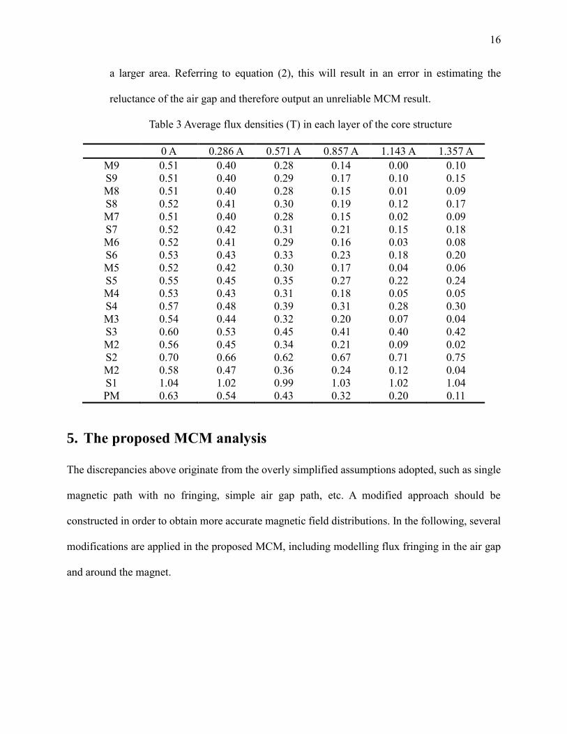
5.1 Modelling of the air gap
Referring to the equation (2) to (5), due to the low permeability of air, the estimation made of the
air gap cross-sectional area can dramatically affect the accuracy of the MCM. A smaller air gap
cross sectional area leads to a higher reluctance value of the air gap element and a lower total
amount of flux. In the conventional MCM, the magnetic flux is assumed to travel through the air
gap along the shortest path, i.e. on straight field lines. However, as shown in Figure 5(a), the flux
travels in an expanded area between the top plate and the yoke. The flux travel path at the air gap
is observed to be about 10 mm wider than the thickness of the yoke. This matches closely with the
air gap model proposed by Roters [39] which is shown in Figure 6(a). In his model, the width of
air gap element between two steel poles of equal width is extended for two times the gap height g.
Although the greater lateral extent of the top plate would increase the actual air gap enlargement
somewhat, the same enlargement of the air gap width on each side by the gap height g is assumed
for the prototype isolator, as illustrated as Figure 6(b). Since the yoke is a tubular component, the
air gap should also be modelled as tubular and its cross-sectional area can be formulated as follows
in terms of the yoke inner and outer diameters:
𝐴airgap = 𝜋 × (∅yoke outer
2+ 𝑔)
2
− 𝜋 × (∅yoke inner
2− 𝑔)
2
(7)
(a) Air gap model proposed by
Roters [39]
(b) Air gap model for the
proposed isolator
Figure 6. Air gap models

18
5.2 MCM with consideration of flux fringing
In addition to the modified air gap model, the modelling of the laminated core structure is also
improved in the proposed MCM method. Considering the vector property of magnetic flux, the
fluxes dispersed in each cylindrical layer in the laminated core structure can be categorised into
two dimensions which are normal flux (Ø) and radial flux (Ø’) as shown in Figure 7. Normal flux
is taken as the flux passing across the disk top surface of each element while radial flux is the flux
leaked out through the side surface of the element in the radial direction. By the principle of
magnetic flux conservation, the difference of the fluxes crossing the top and bottom surfaces of a
layer must equal the flux leaked out the side of the layer. Because the permeability of MRE is
much lower than that of steel and the radial path across the sheets is quite long, the radial flux
leakage for the MRE sheets is ignored, i.e. approximated as 0. The difference in Ø between the
adjacent MRE layers equals the Ø’ of the steel layer in between them. Denoting the total amount
of flux generated by the PM, the normal flux in the ith MRE layer and the leakage flux in the ith
steel layer are denoted as ØPM, Øi and Ø’i respectively, their relationships are represented as
equation (8):
∅PM = ∅1 + ∅1′
(8) ∅𝑖 = ∅𝑖+1 + ∅𝑖+1
′
Figure 7. Normal flux and radial flux (distributed around the disc perimeter)
Accordingly, the proposed MCM is constructed and shown in Figure 8. Since fringing flux is
neglected in all MRE layers, there is only one category of flux component for MRE layers which

19
is Øi. In steel layers, the magnetic flux was separated into two components which are the normal
flux (Øi) and fringing flux (Ø’i). These fringing fluxes leak out at the ith steel layers then travels
through the air path which has the reluctance of Rairi and goes back to the laminated structure
forming the paralleled air reluctance elements in the circuit. The illustration for the flux leakage
paths, i.e., Rair1 and Rair2, are presented in Figure 9. The calculation of Rairi values follows equation
(2). In equation (2), l used is the length of path which crosses the centre of the cross section of Rairi
(presented as red dotted line in Figure 9); and, A is using the cylindrical surface area of the steel
sheet. Since the fringing fluxes leaked out from steel sheet layers in the radial direction, the radial
reluctance of steel sheet (Rsr) is also include in the paralleled fringing path. Rairi values are
summarised in Appendix B. Rsz is the reluctance of steel sheet in the normal direction. Assuming
the flux leakage only occurs at the middle point of the axial height of the steel sheet, for ØPM and
Ø9, they only travel for the half of the 1st and 9th steel sheets respectively on the normal direction.
Figure 8. MCM with considering Magnetic flux fringing effect

20
Figure 9. Flux leakage path
Additionally, to include the influence of fringing flux at air gap between the top plate and the yoke,
the air gap model presented in Figure 6(b) and equation (7) was adopted in this MCM to provide
a more accurate cross-sectional size for air gap. Following Kirchhoff’s law, the mathematical
expression of the proposed MCM can be expressed as equation (9):
By substituting equation (2), (3) and (8) into equation (9), the amount of flux in each layer can be
yielded. To simplify the solving procedure, permeability for steel and MRE is assumed as constant
with µsteel = 3.93 × 10⁻³ Hm-1 and µMRE = 4.73 × 10⁻⁶ Hm-1. This assumption is valid since the flux
densities in all steel components did not reach saturation; as for MRE, the total axial height of
MRE sheets is small, i.e., 18 mm, which has insignificant influence on the result accuracy.
FPM = ØPM
(RPM + RSZ
) + Ø1′ (2RSR
+ Rair1 )
(9)
Ø1′ (2RSR
+ Rair1 ) = Ø2
′ (2RSR + Rair2
) + 2Ø1 (RMRE
+ RSZ )
Ø𝑖′(2RSR
+ Rair𝑖 ) = Ø𝑖+1
′ (2RSR + Rair𝑖+1
) + 2Ø𝑖 (RMRE
+ RSZ )
Fcoil = - Ø9
(RS𝑍 + 2RMRE
+ R𝑎𝑖𝑟𝑔𝑎𝑝 + R𝑆𝑡𝑒𝑒𝑙
) + Ø9′ (2RSR
+ Rair9 )

21
However, the flux density cannot be obtained through Gauss’ Law directly, since the fluxes in the
normal and radial direction for each element should all be considered when calculating flux density.
Considering the vector property of magnetic field, equation (10) should be adopted to obtain the
flux density in steel sheet.
𝐵 = √(Ø𝑖/𝐴𝑛)2 + (Ø𝑖′/𝐴𝑟)22
(10)
Where An and Ar are the areas of the top surface and the side surface of the steel sheet.
6. Results and Discussion
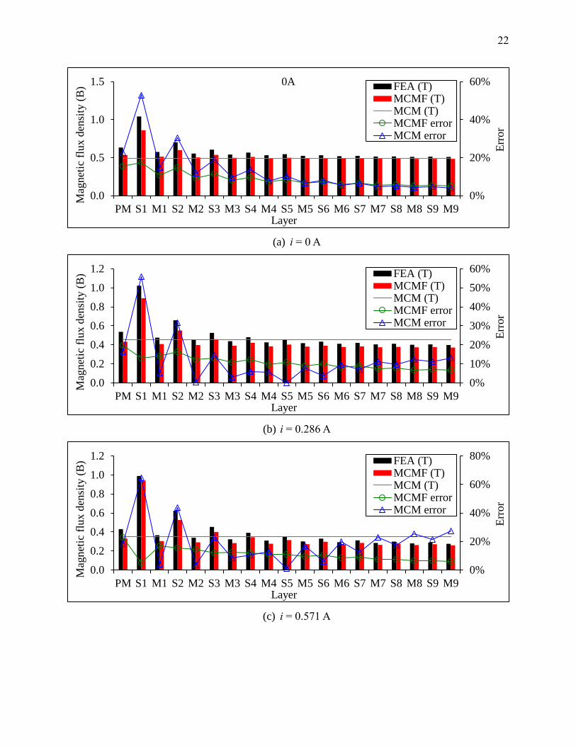
The computed flux density at each layer using FEA, MCM and MCM considering flux fringing
(MCMF) effect is illustrated in Figure 10. The horizontal axis represents the layers of the laminated
core. The results from conventional MCM are represented by the flat grey lines since this method
cannot capture the variances of magnetic field in laminated core structures. The red bar and black
bar represent the results from the improved MCM and FEA. The green line and blue line indicate
the errors of the MCM with considering flux fringing effect and the conventional MCM compared
with FEA in percentage which are calculated through equation (11). Detailed values of magnetic
flux densities and errors are summarised in Table 4.
𝐸𝑟𝑟𝑜𝑟 =𝐴𝐵𝑆(𝑚𝑜𝑑𝑒𝑙 𝑟𝑒𝑠𝑢𝑙𝑡 − 𝐹𝐸𝐴 𝑟𝑒𝑠𝑢𝑙𝑡)
𝐹𝐸𝐴 𝑟𝑒𝑠𝑢𝑙𝑡× 100%
(11)
22
(a) i = 0 A
(b) i = 0.286 A
(c) i = 0.571 A
0%
20%
40%
60%
0.0
0.5
1.0
1.5
PM S1 M1 S2 M2 S3 M3 S4 M4 S5 M5 S6 M6 S7 M7 S8 M8 S9 M9
Err
or
Mag
net
ic f
lux
den
sity
(B
)
Layer
0A FEA (T)MCMF (T)MCM (T)MCMF errorMCM error
0%
10%
20%
30%
40%
50%
60%
0.0
0.2
0.4
0.6
0.8
1.0
1.2
PM S1 M1 S2 M2 S3 M3 S4 M4 S5 M5 S6 M6 S7 M7 S8 M8 S9 M9
Err
or
Mag
net
ic f
lux
den
sity
(B
)
Layer
FEA (T)MCMF (T)MCM (T)MCMF errorMCM error
0%
20%
40%
60%
80%
0.0
0.2
0.4
0.6
0.8
1.0
1.2
PM S1 M1 S2 M2 S3 M3 S4 M4 S5 M5 S6 M6 S7 M7 S8 M8 S9 M9
Err
or
Mag
net
ic f
lux
den
sity
(B
)
Layer
FEA (T)MCMF (T)MCM (T)MCMF errorMCM error

23
(d) i = 0.857 A
(e) i = 1.143 A
(f) i = 1.357 A
Figure 10. Computed flux density for each layer of the laminated structure when different i
applied using FEA, MCM and MCMF (MCM considering fringing effect)
0%
20%
40%
60%
80%
100%
0.0
0.2
0.4
0.6
0.8
1.0
1.2
PM S1 M1 S2 M2 S3 M3 S4 M4 S5 M5 S6 M6 S7 M7 S8 M8 S9 M9
Err
or
Mag
net
ic f
lux
den
sity
(B
)
Layer
FEA (T) MCMF (T)MCM (T) MCMF errorMCM error
0%
500%
1000%
1500%
2000%
0.0
0.2
0.4
0.6
0.8
1.0
1.2
PM S1 M1 S2 M2 S3 M3 S4 M4 S5 M5 S6 M6 S7 M7 S8 M8 S9 M9
Err
or
Mag
net
ic f
lux
den
sity
(B
)
Layer
FEA (T)MCMF (T)MCM (T)MCMF errorMCM error
0%
20%
40%
60%
80%
100%
0.0
0.5
1.0
1.5
PM S1 M1 S2 M2 S3 M3 S4 M4 S5 M5 S6 M6 S7 M7 S8 M8 S9 M9
Err
or
Mag
net
ic f
lux
den
sity
(B
)
Layer
FEA (T)MCMF (T)MCMF error

24
Table 4 Results from FEA, MCM and MCMF (MCM considering fringing effect)
(a) i = 0 A
FEA (T) MCMF (T) MCM (T) MCMF error MCM error
PM 0.63 0.53 0.49 15.7% 22.7%
S1 1.04 0.86 0.49 17.4% 53.0%
M1 0.58 0.51 0.49 10.8% 14.8%
S2 0.70 0.60 0.49 14.8% 30.4%
M2 0.56 0.50 0.49 9.3% 11.7%
S3 0.60 0.54 0.49 11.3% 19.0%
M3 0.54 0.50 0.49 8.1% 9.5%
S4 0.57 0.51 0.49 9.7% 13.6%
M4 0.53 0.49 0.49 7.2% 7.8%
S5 0.55 0.50 0.49 8.4% 10.3%
M5 0.52 0.49 0.49 6.4% 6.5%
S6 0.53 0.49 0.49 7.2% 7.9%
M6 0.52 0.49 0.49 5.9% 5.5%
S7 0.52 0.49 0.49 6.5% 6.4%
M7 0.51 0.49 0.49 5.4% 4.7%
S8 0.52 0.49 0.49 5.7% 5.2%
M8 0.51 0.49 0.49 5.1% 4.2%
S9 0.51 0.49 0.49 5.5% 4.6%
M9 0.51 0.48 0.49 4.9% 3.9%
(b) i = 0.286 A
FEA (T) MCMF (T) MCM (T) MCMF error MCM error
PM 0.54 0.43 0.45 19.6% 16.2%
S1 1.02 0.89 0.45 13.0% 56.0%
M1 0.47 0.41 0.45 14.0% 5.2%
S2 0.66 0.55 0.45 16.3% 31.6%
M2 0.45 0.40 0.45 12.2% 0.5%
S3 0.53 0.46 0.45 12.9% 14.5%
M3 0.44 0.39 0.45 10.9% 2.9%
S4 0.48 0.42 0.45 12.1% 6.1%
M4 0.43 0.38 0.45 9.7% 5.6%
S5 0.45 0.40 0.45 10.8% 0.1%
M5 0.42 0.38 0.45 8.8% 7.8%
S6 0.43 0.39 0.45 9.9% 3.8%
M6 0.41 0.38 0.45 8.0% 9.6%
S7 0.42 0.38 0.45 8.7% 7.0%
M7 0.40 0.38 0.45 7.3% 11.1%
S8 0.41 0.38 0.45 7.8% 9.5%
M8 0.40 0.37 0.45 6.8% 12.3%
S9 0.40 0.38 0.45 7.1% 11.3%
M9 0.40 0.37 0.45 6.6% 13.1%
25
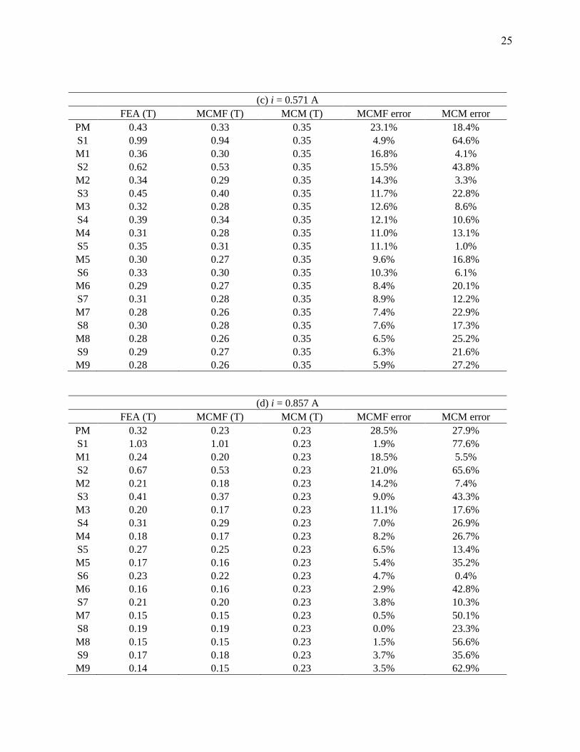
(c) i = 0.571 A
FEA (T) MCMF (T) MCM (T) MCMF error MCM error
PM 0.43 0.33 0.35 23.1% 18.4%
S1 0.99 0.94 0.35 4.9% 64.6%
M1 0.36 0.30 0.35 16.8% 4.1%
S2 0.62 0.53 0.35 15.5% 43.8%
M2 0.34 0.29 0.35 14.3% 3.3%
S3 0.45 0.40 0.35 11.7% 22.8%
M3 0.32 0.28 0.35 12.6% 8.6%
S4 0.39 0.34 0.35 12.1% 10.6%
M4 0.31 0.28 0.35 11.0% 13.1%
S5 0.35 0.31 0.35 11.1% 1.0%
M5 0.30 0.27 0.35 9.6% 16.8%
S6 0.33 0.30 0.35 10.3% 6.1%
M6 0.29 0.27 0.35 8.4% 20.1%
S7 0.31 0.28 0.35 8.9% 12.2%
M7 0.28 0.26 0.35 7.4% 22.9%
S8 0.30 0.28 0.35 7.6% 17.3%
M8 0.28 0.26 0.35 6.5% 25.2%
S9 0.29 0.27 0.35 6.3% 21.6%
M9 0.28 0.26 0.35 5.9% 27.2%
(d) i = 0.857 A
FEA (T) MCMF (T) MCM (T) MCMF error MCM error
PM 0.32 0.23 0.23 28.5% 27.9%
S1 1.03 1.01 0.23 1.9% 77.6%
M1 0.24 0.20 0.23 18.5% 5.5%
S2 0.67 0.53 0.23 21.0% 65.6%
M2 0.21 0.18 0.23 14.2% 7.4%
S3 0.41 0.37 0.23 9.0% 43.3%
M3 0.20 0.17 0.23 11.1% 17.6%
S4 0.31 0.29 0.23 7.0% 26.9%
M4 0.18 0.17 0.23 8.2% 26.7%
S5 0.27 0.25 0.23 6.5% 13.4%
M5 0.17 0.16 0.23 5.4% 35.2%
S6 0.23 0.22 0.23 4.7% 0.4%
M6 0.16 0.16 0.23 2.9% 42.8%
S7 0.21 0.20 0.23 3.8% 10.3%
M7 0.15 0.15 0.23 0.5% 50.1%
S8 0.19 0.19 0.23 0.0% 23.3%
M8 0.15 0.15 0.23 1.5% 56.6%
S9 0.17 0.18 0.23 3.7% 35.6%
M9 0.14 0.15 0.23 3.5% 62.9%

26
(e) i = 1.143 A
FEA (T) MCMF (T) MCM (T) MCMF error MCM error
PM 0.20 0.13 0.09 37.0% 55.1%
S1 1.02 1.09 0.09 7.2% 91.1%
M1 0.12 0.09 0.09 24.4% 27.3%
S2 0.71 0.56 0.09 21.1% 87.2%
M2 0.09 0.08 0.09 12.3% 2.5%
S3 0.40 0.37 0.09 6.2% 77.4%
M3 0.07 0.07 0.09 0.9% 35.1%
S4 0.28 0.28 0.09 0.5% 67.8%
M4 0.05 0.06 0.09 13.7% 77.2%
S5 0.22 0.23 0.09 3.1% 58.8%
M5 0.04 0.05 0.09 34.1% 135.9%
S6 0.18 0.19 0.09 4.5% 49.9%
M6 0.03 0.05 0.09 65.1% 224.9%
S7 0.15 0.16 0.09 6.6% 40.3%
M7 0.02 0.04 0.09 119.2% 380.4%
S8 0.12 0.14 0.09 13.0% 27.6%
M8 0.01 0.04 0.09 227.2% 695.9%
S9 0.10 0.12 0.09 28.2% 7.4%
M9 0.00 0.03 0.09 572.5% 1712.5%
(f) i = 1.357 A
FEA (T) MCMF (T) MCM (T) MCMF error MCM error
PM 0.11 0.05 0.00 55.7%
Not applicable
S1 1.04 1.16 0.00 11.4%
M1 0.04 0.01 0.00 65.4%
S2 0.75 0.59 0.00 21.2%
M2 0.02 0.00 0.00 81.3%
S3 0.42 0.40 0.00 5.4%
M3 0.04 0.01 0.00 58.5%
S4 0.30 0.30 0.00 1.4%
M4 0.05 0.02 0.00 53.8%
S5 0.24 0.24 0.00 2.3%
M5 0.06 0.03 0.00 51.9%
S6 0.20 0.21 0.00 1.1%
M6 0.08 0.04 0.00 50.9%
S7 0.18 0.18 0.00 2.4%
M7 0.09 0.04 0.00 50.3%
S8 0.17 0.16 0.00 3.3%
M8 0.09 0.05 0.00 49.9%
S9 0.15 0.15 0.00 1.5%
M9 0.10 0.05 0.00 49.6%

27
As shown in Figure 10(a), for the scenario with no current applied, the overall error for all layers
of the laminated core obtained from the proposed MCM and the conventional MCM are 8.71%
and 12.73%. The proposed MCM can well portray the variance of magnetic field in different layers
and the excessively high flux density values in the first 3 steel layers which are 1.02 T, 0.78 T and
0.64 T respectively, with error within 12%. For MRE layers, the average error of the proposed
MCM is 7.02%. The maximum and minimum flux density values in MRE are 0.51 T and 0.48 T
for the 1st and the 9th MRE layers well matched with FEA results. The maximum error of flux
densities value between the proposed MCM and FEA is only 0.18 T, however, that of the
conventional MCM is 0.55 T.
By increasing the applied i to 1.143 A, as illustrated in Figure 10(e), the overall error of the
proposed MCM increased to 63.00%. Nevertheless, the overall error of conventional MCM soared
to 202.86%. The magnetic flux density in the PM was effectively reduced from 0.53 T to 0.13 T
when the applied i increased from 0 to 1.143 A, according to the improved MCM. At this scenario,
although the percentage error increased due to the decrease of base number, the maximum error of
flux density value between the improved MCM and FEA is only of 0.15 T (0.93 T for the
conventional method). It can be concluded that the improved MCM can effectively capture the
electromagnetic performance of the device when different i is applied.
With the increase of the applied current to the coil, the flux density in MRE layers decreases,
however, flux fringing effect at the laminated core still exhibits eminent flux density values in the
steel layers. Additionally, the difference between flux densities of steel and MRE layers became
more noticeable when larger current was applied, especially for the layer adjacent to the PM. The
computed improved MCM can well reproduce this behaviour. For example, for the first steel layer,
28
it yields 0.86 T, 0.89 T, 0.93 T, 1.01 T and 1.09 T for applied i increased from 0 A to 1.143 A with
the overall error less than 9%. On the contrary, conventional MCM reached almost 70% error for
these five scenarios. With further increase of the applied current to 1.357 A, which is the scenario
that the conventional MCM failed to compute, the proposed MCM still achieves a high accuracy
with overall percentage error of 32% and maximum error of flux density value of 0.16 T.
Compared with available results from FEA and the conventional MCM, the effectiveness and
superiority of the proposed MCM in depicting the magnetic flux density for the hybrid magnets
laminated core and flux fringing effect have been revealed.
7. Further discussion
7.1 Experimental validation of magnetic field
In the real design of laminated MRE-based adaptive devices, currently, the magnetic field in the
laminated structure can only be estimated by FEA and MCM; and, there is no sensor available to
directly measure the field distribution inside of a laminated structure without damaging the
structure and changing the flux path. Therefore, developing a rapid and accurate MCM is of great
significance addressing the structural complexity of laminated MRE-based devices.
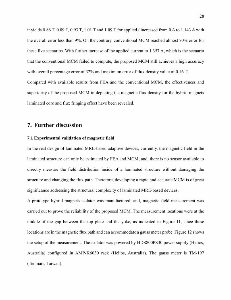
A prototype hybrid magnets isolator was manufactured; and, magnetic field measurement was
carried out to prove the reliability of the proposed MCM. The measurement locations were at the
middle of the gap between the top plate and the yoke, as indicated in Figure 11, since these
locations are in the magnetic flux path and can accommodate a gauss meter probe. Figure 12 shows
the setup of the measurement. The isolator was powered by HDS800PS30 power supply (Helios,
Australia) configured in AMP-K6030 rack (Helios, Australia). The gauss meter is TM-197
(Tenmars, Taiwan).

29
Figure 11. Measurement positions
Figure 12. Measurement setup and gaussmeter
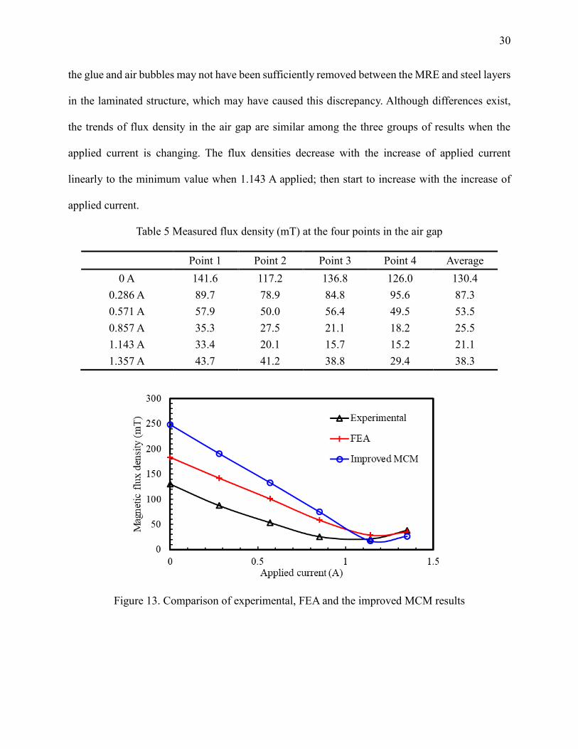
The measured magnetic flux density values are summarised in Table 5. The average measured flux
density of the four locations and the results of flux density in the air gap from the improved MCM
and FEA results are plotted in Figure 13. The FEA results were taken at the middle point of the top
plate and the yoke. The measured value is lower than both the FEA result and the improved MCM.
A similar phenomenon has been reported by Li et al [11]. The major reason of having lower
experimental values is that the bonding surfaces of the laminated structure were not considered in
theoretical methods. The bonding of the MRE and steel layers in the real device is not as perfect
as that in theoretical methods. In the 37-layer structure, there are 38 layers of adhesive applied and
30
the glue and air bubbles may not have been sufficiently removed between the MRE and steel layers
in the laminated structure, which may have caused this discrepancy. Although differences exist,
the trends of flux density in the air gap are similar among the three groups of results when the
applied current is changing. The flux densities decrease with the increase of applied current
linearly to the minimum value when 1.143 A applied; then start to increase with the increase of
applied current.
Table 5 Measured flux density (mT) at the four points in the air gap
Point 1 Point 2 Point 3 Point 4 Average
0 A 141.6 117.2 136.8 126.0 130.4
0.286 A 89.7 78.9 84.8 95.6 87.3
0.571 A 57.9 50.0 56.4 49.5 53.5
0.857 A 35.3 27.5 21.1 18.2 25.5
1.143 A 33.4 20.1 15.7 15.2 21.1
1.357 A 43.7 41.2 38.8 29.4 38.3
Figure 13. Comparison of experimental, FEA and the improved MCM results

31
7.2 Recommendations on the design of isolator with hybrid magnetic
As for optimization of hybrid magnet systems in the adaptive isolators with laminated MRE core
structure, the selection and positioning of the PM and the configuration of coil are critical. For PM,
according to suggestions from [40], realising the maximum magnetic energy product is preferred
in order to make the volume of PM smallest and to give the highest efficacy of electromagnetic
performance of the device. For a neodymium magnet, since its demagnetization curve is a straight
line in the second quadrant, the max magnetic energy product can be reached when the magnetic
flux density in the magnet is half of its remanence. According to the improved MCM, in the
prototype device, the magnetic flux density in the PM is 0.61 T when no current applied to the coil.
Since this value is around half of the remanence of an N40 neodymium magnet, e.g. 1.25 T, this
device accomplished a most effective and compact configuration. Regarding the positioning of the
PM, the design proposed used one layer in the middle of the laminated core structure rather than
separating the PM into several thinner layers. This is to protect the PM from irrecoverable
demagnetization when the coil is energised and also to avoid cracking of PM due to its brittle
nature. The design of the coil should provide sufficient MMF to offset the magnetic field from the
PM.
8. Summary
In this work, a novel MRE-based adaptive isolator featuring stiffness softening effect and an
improved MCM has been proposed. Also, suggestions addressing the application of the hybrid
magnet system were provided. Considering the magnetic field dependence of this device,
theoretical analysis including conventional MCM and FEA have been conducted. FEA results
revealed that the proposed device provides a wide range of controllability of magnetic field, which

32
can be offset to almost 0 T from 0.57 T in MRE layers when 1.357 A is applied to each small coil,
therefore offering outstanding adjustability in the mechanical properties. By addressing the flux
fringing effects the proposed MCM achieves excellence in capturing the magnetic field distribution
localized to each layer in the laminated structure for both non-current applied and large current
applied scenarios. The proposed MCM also mitigated the failure of computing the maximum
current applied scenario for the conventional MCM.
Reference
[1] Ginder, J. M., Clark, S. M., Schlotter, W. F., & Nichols, M. E. (2002). Magnetostrictive
phenomena in magnetorheological elastomers. International Journal of Modern Physics
B, 16(17n18), 2412-2418.
[2] Behrooz, M., Wang, X., & Gordaninejad, F. (2014). Performance of a new
magnetorheological elastomer isolation system. Smart Materials and Structures, 23(4),
045014.
[3] Jung, H. J., Eem, S. H., Jang, D. D., & Koo, J. H. (2011). Seismic performance analysis of
a smart base-isolation system considering dynamics of MR elastomers. Journal of
Intelligent Material Systems and Structures, 22(13), 1439-1450.
[4] Ginder, J. M., Schlotter, W. F., & Nichols, M. E. (2001, July). Magnetorheological
elastomers in tunable vibration absorbers. In Smart Structures and Materials 2001:
Damping and Isolation (Vol. 4331, pp. 103-110). International Society for Optics and
Photonics.
33
[5] Xu, Z., Gong, X., Liao, G., & Chen, X. (2010). An active-damping-compensated
magnetorheological elastomer adaptive tuned vibration absorber. Journal of Intelligent
Material Systems and Structures, 21(10), 1039-1047.
[6] Yun, G., Tang, S. Y., Sun, S., Yuan, D., Zhao, Q., Deng, L., ... & Li, W. (2019). Liquid
metal-filled magnetorheological elastomer with positive piezoconductivity. Nature
Communications, 10(1), 1300.
[7] Qi, S., Guo, H., Chen, J., Fu, J., Hu, C., Yu, M., & Wang, Z. L. (2018). Magnetorheological
elastomers enabled high-sensitive self-powered tribo-sensor for magnetic field
detection. Nanoscale, 10(10), 4745-4752.
[8] Thorsteinsson, F., Gudmundsson, I., & Lecomte, C. (2015). U.S. Patent No. 9,078,734.
Washington, DC: U.S. Patent and Trademark Office.
[9] Yang, T., Xie, D., Li, Z., & Zhu, H. (2017). Recent advances in wearable tactile sensors:
Materials, sensing mechanisms, and device performance. Materials Science and
Engineering: R: Reports, 115, 1-37.
[10] Li, Y., & Li, J. (2019). Overview of the development of smart base isolation system
featuring magnetorheological elastomer. Smart Structures and Systems, 24(1), 37-52.
[11] Li, Y., Li, J., Li, W., & Samali, B. (2013). Development and characterization of a
magnetorheological elastomer based adaptive seismic isolator. Smart Materials and
Structures, 22(3), 035005.
[12] Li, Y., Li, J., Tian, T., & Li, W. (2013). A highly adjustable magnetorheological
elastomer base isolator for applications of real-time adaptive control. Smart Materials and
Structures, 22(9), 095020.
34
[13] Gu, X., Li, J., & Li, Y. (2020). Experimental realisation of the real‐time controlled
smart magnetorheological elastomer seismic isolation system with shake table. Structural
Control and Health Monitoring, 27(1), e2476.
[14] Xing, Z. W., Yu, M., Fu, J., Wang, Y., & Zhao, L. J. (2015). A laminated
magnetorheological elastomer bearing prototype for seismic mitigation of bridge
superstructures. Journal of Intelligent Material Systems and Structures, 26(14), 1818-1825.
[15] Yu, M., Zhao, L., Fu, J., & Zhu, M. (2016). Thermal effects on the laminated
magnetorheological elastomer isolator. Smart Materials and Structures, 25(11), 115039.
[16] Yang, J., Sun, S. S., Du, H., Li, W. H., Alici, G., & Deng, H. X. (2014). A novel
magnetorheological elastomer isolator with negative changing stiffness for vibration
reduction. Smart Materials and Structures, 23(10), 105023.
[17] Sun, S., Deng, H., Yang, J., Li, W., Du, H., Alici, G., & Nakano, M. (2015). An
adaptive tuned vibration absorber based on multilayered MR elastomers. Smart Materials
and Structures, 24(4), 045045.
[18] Kashima, S., Miyasaka, F., & Hirata, K. (2012). Novel soft actuator using
magnetorheological elastomer. IEEE Transactions on Magnetics, 48(4), 1649-1652.
[19] Yang, G., Spencer Jr, B. F., Carlson, J. D., & Sain, M. K. (2002). Large-scale MR
fluid dampers: modeling and dynamic performance considerations. Engineering
Structures, 24(3), 309-323.
[20] Chen, C., & Liao, W. H. (2012). A self-sensing magnetorheological damper with
power generation. Smart Materials and Structures, 21(2), 025014.
[21] Milecki, A. (2001). Investigation and control of magneto–rheological fluid
dampers. International Journal of Machine Tools and Manufacture, 41(3), 379-391.

35
[22] Zheng, J., Li, Z., Koo, J., & Wang, J. (2014). Magnetic circuit design and
multiphysics analysis of a novel MR damper for applications under high velocity. Advances
in Mechanical Engineering, 6, 402501.
[23] Zhu, X., Jing, X., & Cheng, L. (2012). Magnetorheological fluid dampers: a review
on structure design and analysis. Journal of Intelligent Material Systems and
Structures, 23(8), 839-873.
[24] Yang, B., Luo, J., & Dong, L. (2010). Magnetic circuit FEM analysis and optimum
design for MR damper. International Journal of Applied Electromagnetics and
Mechanics, 33(1-2), 207-216.
[25] Gavin, H., Hoagg, J., & Dobossy, M. (2001, August). Optimal design of MR
dampers. In Proceedings of the US-Japan Workshop on Smart Structures for Improved
Seismic Performance in Urban Regions (Vol. 14, pp. 225-236).
[26] Takesue, N., Furusho, J., & Kiyota, Y. (2004). Fast response MR-fluid
actuator. JSME International Journal Series C Mechanical Systems, Machine Elements
and Manufacturing, 47(3), 783-791.
[27] An, J., & Kwon, D. S. (2003). Modeling of a magnetorheological actuator including
magnetic hysteresis. Journal of Intelligent Material Systems and Structures, 14(9), 541-
550.
[28] Boelter, R., & Janocha, H. (1997, May). Design rules for MR fluid actuators in
different working modes. In Smart Structures and Materials 1997: Passive Damping and
Isolation (Vol. 3045, pp. 148-160). International Society for Optics and Photonics.
36
[29] Yoo, J. H., & Wereley, N. M. (2002). Design of a high-efficiency
magnetorheological valve. Journal of Intelligent Material Systems and Structures, 13(10),
679-685.
[30] Grunwald, A., & Olabi, A. G. (2008). Design of magneto-rheological (MR)
valve. Sensors and Actuators A: Physical, 148(1), 211-223.
[31] Guo, N. Q., Du, H., & Li, W. H. (2003). Finite element analysis and simulation
evaluation of a magnetorheological valve. The International Journal of Advanced
Manufacturing Technology, 21(6), 438-445.
[32] Nguyen, Q. H., Han, Y. M., Choi, S. B., & Wereley, N. M. (2007). Geometry
optimization of MR valves constrained in a specific volume using the finite element
method. Smart Materials and Structures, 16(6), 2242.
[33] Wang, Q., Dong, X., Li, L., & Ou, J. (2018). Mechanical modeling for
magnetorheological elastomer isolators based on constitutive equations and
electromagnetic analysis. Smart Materials and Structures, 27(6), 065017.
[34] Xing, Z. W., Yu, M., Fu, J., Wang, Y., & Zhao, L. J. (2015). A laminated
magnetorheological elastomer bearing prototype for seismic mitigation of bridge
superstructures. Journal of Intelligent Material Systems and Structures, 26(14), 1818-1825.
[35] Zhou, G. Y. (2003). Shear properties of a magnetorheological elastomer. Smart
Materials and Structures, 12(1), 139.
[36] Zhou, G. Y., & Li, J. R. (2003). Dynamic behavior of a magnetorheological
elastomer under uniaxial deformation: I. Experiment. Smart Materials and
Structures, 12(6), 859.

37
[37] Böse, H., Rabindranath, R., & Ehrlich, J. (2012). Soft magnetorheological
elastomers as new actuators for valves. Journal of Intelligent Material Systems and
Structures, 23(9), 989-994.
[38] Yang, C. Y., Fu, J., Yu, M., Zheng, X., & Ju, B. X. (2015). A new
magnetorheological elastomer isolator in shear–compression mixed mode. Journal of
Intelligent Material Systems and Structures, 26(10), 1290-1300.
[39] Roters, H. C. (1941). Electromagnetic devices. Wiley.
[40] Wright, W., & McCaig, M. (1977). Permanent Magnets. Oxford University Press
for the Design Council, the British Standards Institution, and the Council of Engineering
Institutions.

38
Appendix A
𝑙air = ℎ𝑒𝑖𝑔ℎ𝑡 𝑜𝑓 𝑎𝑖𝑟𝑔𝑎𝑝 = 5 mm
𝑙MRE = 𝑡ℎ𝑖𝑐𝑘𝑛𝑒𝑠𝑠 𝑜𝑓 𝑀𝑅𝐸 = 1 mm
𝑙Steel sheet = 𝑡ℎ𝑖𝑐𝑘𝑛𝑒𝑠𝑠 𝑜𝑓 𝑠𝑡𝑒𝑒𝑙 𝑠ℎ𝑒𝑒𝑡 = 1 mm
𝑙Steel block = ℎ𝑒𝑖𝑔ℎ𝑡 𝑜𝑓 𝑠𝑡𝑒𝑒𝑙 𝑏𝑙𝑜𝑐𝑘 = 37 mm
𝑙Yoke = ℎ𝑒𝑖𝑔ℎ𝑡 𝑜𝑓 𝑦𝑜𝑘𝑒 = 110 mm
𝑙PM = 𝑡ℎ𝑖𝑐𝑘𝑛𝑒𝑠𝑠 𝑜𝑓 𝑃𝑀 = 5 mm
𝑙Steel plate = ℎ𝑎𝑙𝑓 𝑜𝑓 𝑡ℎ𝑒 𝑝𝑙𝑎𝑡𝑒 𝑡ℎ𝑖𝑐𝑘𝑛𝑒𝑠𝑠 × 2
+ 𝐴𝑣𝑒𝑟𝑎𝑔𝑒 𝑜𝑓𝑖𝑛𝑛𝑒𝑟 𝑎𝑛𝑑 𝑜𝑢𝑡𝑒𝑟 𝑟𝑎𝑑𝑖𝑢𝑠 𝑜𝑓 𝑦𝑜𝑘𝑒 = 110 mm
𝐴air = 𝜋(𝑜𝑢𝑡𝑒𝑟 𝑟𝑎𝑑𝑖𝑢𝑠 𝑜𝑓 𝑦𝑜𝑘𝑒)2 − 𝜋(𝑖𝑛𝑛𝑒𝑟 𝑟𝑎𝑑𝑖𝑢𝑠 𝑜𝑓 𝑦𝑜𝑘𝑒)2 = 12566.37 mm2
𝐴MRE = 𝜋(𝑟𝑎𝑑𝑖𝑢𝑠 𝑜𝑓 𝑀𝑅𝐸)2 = 7853.98 mm2
𝐴Steel sheet = 𝜋(𝑟𝑎𝑑𝑖𝑢𝑠 𝑜𝑓 𝑠𝑡𝑒𝑒𝑙 𝑠ℎ𝑒𝑒𝑡)2 = 7853.98 mm2
𝐴Steel block = 𝜋(𝑟𝑎𝑑𝑖𝑢𝑠 𝑜𝑓 𝑠𝑡𝑒𝑒𝑙 𝑏𝑙𝑜𝑐𝑘)2 = 7853.98 mm2
𝐴Yoke = 𝜋(𝑜𝑢𝑡𝑒𝑟 𝑟𝑎𝑑𝑖𝑢𝑠 𝑜𝑓 𝑦𝑜𝑘𝑒)2 − 𝜋(𝑖𝑛𝑛𝑒𝑟 𝑟𝑎𝑑𝑖𝑢𝑠 𝑜𝑓 𝑦𝑜𝑘𝑒)2 = 12566.37 mm2
𝐴PM = 𝜋(𝑟𝑎𝑑𝑖𝑢𝑠 𝑜𝑓 𝑃𝑀)2 = 7853.98 mm2
𝐴Steel plate = (𝑝𝑙𝑎𝑡𝑒 𝑡ℎ𝑖𝑐𝑘𝑛𝑒𝑠𝑠) × 𝜋(𝑑𝑖𝑎𝑚𝑒𝑡𝑒𝑟 𝑜𝑓 𝑠𝑡𝑒𝑒𝑙 𝑏𝑙𝑜𝑐𝑘
+ 𝑖𝑛𝑛𝑒𝑟 𝑑𝑖𝑎𝑚𝑒𝑡𝑒𝑟 𝑜𝑓 𝑦𝑜𝑘𝑒)/2 = 4398.23 mm2

39
Appendix B
Reluctance of fringing path
l (m) A (m2) R (Aturns/Wb)
Rair1 6.57E-03 3.14E-04 1.66E+07
Rair2 1.29E-02 3.14E-04 3.25E+07
Rair3 1.91E-02 3.14E-04 4.84E+07
Rair4 2.54E-02 3.14E-04 6.43E+07
Rair5 3.17E-02 3.14E-04 8.02E+07
Rair6 3.80E-02 3.14E-04 9.62E+07
Rair7 4.43E-02 3.14E-04 1.12E+08
Rair8 5.06E-02 3.14E-04 1.28E+08
Rair9 5.68E-02 3.14E-04 1.44E+08