improved dynamic emulation modelling by time series ... · posto si basa sull’utilizzo di un...
TRANSCRIPT

Politecnico di Milano
Facolta di Ingegneria Civile, Ambientale e Territoriale
Polo Territoriale di Como
Master of Science in
Environmental and Land Planning Engineering
Improved dynamic emulation modelling bytime series clustering: the case study of
Marina Reservoir, Singapore
Supervisor:
Prof. Andrea Castelletti
Assistant supervisor:
Dr. Stefano Galelli
Master graduation thesis by:
Stefania Caietti Marin
Student Id. number: 745854
Academic Year: 2011-2012


Politecnico di Milano
Facolta di Ingegneria Civile, Ambientale e Territoriale
Polo Territoriale di Como
Corso di Laurea Specialistica in
Ingegneria per l’Ambiente e il Territorio
Dynamic Emulation Modelling e TimeSeries Clustering: il caso di studio di
Marina Reservoir, Singapore
Relatore:
Prof. Andrea Castelletti
Correlatore:
Dr. Stefano Galelli
Tesi di Laurea di:
Stefania Caietti Marin
Matricola: 745854
Anno Accademico: 2011-2012


”Fanciullino, tu sei savio: non vuoi ripetere il gia detto, ne trovare l’indicibile.
Sai che nelle cose e il nuovo, per chi sa vederlo; e non t’indurrai a trovarlo,
affatturando e sofisticando. Il nuovo non s’inventa: si scopre.”
— Giovanni Pascoli
I


Acknowledgements
This master thesis was carried out under the supervision of Andrea Castelletti and
the co-supervision of Stefano Galelli. I wish to thank them for the opportunity
they gave me, and for being great advisors. Their ideas and support had a major
influence on this work.
The case study described in this thesis was developed in collaboration with the
Singapore-Delft Water Alliance (SDWA) at the National University of Singapore
(Singapore), as part of the Multi-objective Multiple-Reservoir Management research
program. I want to express gratitude to all SDWA staff, in particular to Vladan
Babovic, who gave me the possibility of visiting SDWA and working there on the
project activities.
I wish to thank Albert Goedbloed for his special advices and for his active help with
the use of Matlab and I am grateful to Abhay, Ali, Samuel, Phil, Jingjie, and Javier
for having been cooperative fellows and dear friends.
The first loving thanks goes to my family for having been close to me throughout my
studies. A special thanks is for Donata because day by day she encourages me not
to turn away from the truth, and to Serena for her unreserved support, especially
during the most difficult moments.
Thanks also to Paola, Monia, Anna, Annina, Renee, and Maria, as with them I
receive only affection and comprehension, even when I show the worst side of me.
I wish to thank Federica, who came into my life only by accident; she is a really
precious person and I cannot forget what we shared in Singapore.
Thanks also to Trisha, Bokyung, Katja, Anna, Manhang, Hoi Yin, Przemyslaw, An-
drew, David, Tae-Kyu, Karol, Baris, Maggie, Yevgeniy, Tommy, Stephanie, Pawel,
and Konstantin as they made my staying in Asia delightful and amusing: with them
I went through lots of new experiences and I saw magnificent and enchanting places
that I will keep in mind for the rest of my life.
III

I also wish to thank Roberto for having been a constant presence during the prepa-
ration of the exams and the redaction of this thesis, and I am particularly grateful
to all the students that passed me by during these years, as they made me reflect
upon how I was in the past and they made me realize what I want to be in the
future.
My final thanks is for Paolo, who is by my side in this special moment. Maybe I
don’t know what love means; but if it has to do with the encouragement helping the
other to reach a goal, if it implies respect and freedom to express one’s own nature
every single day, then I can say I do love you.
IV


Abstract
Dynamic Emulation Modelling (DEMo) is emerging as a viable solution to combine
computationally intensive simulation models and dynamic optimization algorithms.
A dynamic emulator is a low order surrogate of the simulation model identified over
a sample data set generated by the original simulation model itself. When applied
to large 3D models, any DEMo exercise does require a preprocessing of the exoge-
nous drivers and state variables in order to reduce, by spatial aggregation, the high
number of candidate variables to appear in the final emulator. This work describes
a hybrid clustering-variable selection approach to automatically discover compact
and relevant representations of high-dimensional data sets. Time series clustering
(Liao, 2005) is adopted to identify spatial structures by objectively organizing data
into homogenous groups, where the within-group-object similarity is minimized. In
particular, the proposed approach relies on a hierachical agglomerative clustering
method (Magni et al., 2008), which starts by placing each time-series in its own
cluster, and then merges clusters into larger clusters, until a compact, yet informa-
tive, representation of the original variables can be processed with the Recursive
Variable Selection - Iterative Input Selection algorithm (Castelletti et al., 2011), in
order to single out the most relevant clusters. The approach is demonstrated on a
real-world case study concerning the reduction of DELFT3D, a spatially distributed
hydrodynamic model used to simulate salt intrusion dynamics in a tropical lake
(Marina Reservoir, Singapore).
VII
Sommario
Il Dynamic Emulation Modelling (DEMo) sta emergendo come possibile soluzione
per un utilizzo combinato di algoritmi di ottimizzazione dinamica e di modelli di
simulazione onerosi dal punto di vista computazionale. Un dinamic emulator e
un modello semplificato e computazionalmente efficiente, di un modello di simu-
lazione e puo essere generato tramite simulazione a partire da un campione di dati
prodotto dal modello originale. Se applicato a grandi modelli 3D, l’implementazione
della procedura DEMo richiede un una preliminare trasformazione dei vettori degli
ingressi esogeni e delle variabili di stato per ridurre, attraverso un’aggregazione
spaziale, l’elevato numero di variabili candidate ad apparire nell’emulation model
finale. Questo lavoro di tesi descrive un approccio combinato di techiche di cluster-
izzazione e di variable selection per scoprire in maniera automatica rappresentazioni
compatte e rilevanti in data-set di grandi dimensioni. La clusterizzazione di serie
temporali e qui adottata per identificare in modo oggettivo strutture spaziali nei
dati e per organizzarli in gruppi omogenei, in cui il grado di similarita tra oggetti
appartenenti ad uno stesso gruppo sia massimizzato. In particolare, l’approccio pro-
posto si basa sull’utilizzo di un metodo di clusterizzazione gerarchico agglomerativo,
che inizialmente pone ogni serie temporale in cluster differenti e successivamente li
unisce in cluster di dimensioni sempre maggiori, fino a che una rappresentazione com-
patta, ma informativa, delle variabili originali puo essere processata con l’algoritmo
di Recursive Variable Selection - Iterative Input Selection, al fine di individuare i
cluster piu rilevanti. L’approccio e dimostrato su un caso studio reale riguardante
la riduzione di Delft3D, un modello idrodinamico spazialmente distribuito utiliz-
zato per simulare la dinamica dell’intrusione salina in un lago tropicale (Marina
Reservoir, Singapore).
VIII
Introduction
Advances in scientific computation and data collection techniques have increased the
level of fundamental understanding that can be built into physically-based models,
which are widely adopted to describe the dynamics of large environmental systems.
These models, which are more and more realistic and complex, are often used also to
support planning and management interventions. However, the practical application
of a decision-making scheme in environmental problems can be particularly difficult
as the physically-based models used to describe environmental systems are computa-
tionally intensive and thus ill-suited to support optimization-based decision-making,
which normally requires hundreds or thousands of model evaluations.
A potentially effective approach to overcome these limitations is to perform a top-
down reduction of the physically-based model by a simplified, computationally-
efficient emulation model (Castelletti et al. (2012b) and references therein) con-
structed from and then used in place of the original physically-based model in highly
resource-demanding tasks. The underlying idea is that not all the process details
in the original model are equally important and relevant to the dynamic behaviours
that result into an actual change in the values of the planning/management objec-
tives of the decision-making problem, and thus affect the final decision.
Literature shows a variety of alternate emulation modelling approaches that explored
different knowledge areas and engineering applications, including aeronautics, chem-
ical engineering, robotics, electronics, and micro-engineering. Most of these methods
tend to derive an emulator trying to exploit some peculiar features of the system
under study, or are model-specific, in the sense that the type of emulator depends
upon the type of physically-based model. Moreover, for decision-making problems
(i.e. optimal control) the emulator must be dynamic, that is it must reproduce the
trajectories over any specified horizon of the relevant variables. A shared theoreti-
cal vision is still missing and different techniques were independently developed in
IX

different domain of interest.
Castelletti et al. (2012a) re-organized the techniques adopted in environmental prob-
lems into a general framework to Dynamic Emulation Modelling (DEMo) and dis-
tinguished two categories of dynamic emulators: structure-driven and data-driven.
The former are based on the idea of projecting the high-dimension equations of the
physically-based models onto a lower-dimension space, where the model equations
are solved for the substituted projected states. The latter are generally based on
the identification of the emulator as an I/O relationship over a data set of input-
output samples generated from the original physically-based model. The choice for
one approach or the other depends on the level of complexity and non-linearities
embedded into the original model.
Structure-driven dynamic emulators are well developed for linear, quadratic, and
weakly non-linear models, while theory is still under development for non-linear
models. This category of emulators is also naturally in the state-space form, which
makes it directly and more effectively usable in any management problem. On the
contrary, data-driven emulators can be easily applied to both linear and non-linear
models, as they do not require any analytical assumption about the physically-based
model structure. The resulting emulator, however, is in external form and, generally,
must be converted into state-space form by solving a minimal realization problem,
which can turn out particularly difficult in the non-linear case. Moreover, while lit-
erature shows some operational examples of emulators in external form interpretable
in physical terms (see, for example, GAINS model (Amann, 2009) in the part related
to climate change and air quality emulators), in the water resources sector both the
original external form and the associated minimal realization typically lack of cred-
ibility by stakeholders and domain experts, apart from few particular cases (Young
(1998); See et al. (2008); Babovic (2009)). Data-driven DEMo has been more ex-
tensively explored than its structure-driven twin in environmental modelling, where
systems are typically complex and highly non-linear.
Lately, Castelletti et al. (2012) proposed a new data driven approach that preserves
the internal representation of the original model and allows to get insight on the
physical functioning of the emulator.
The purpose of my thesis is to enhance the status of these techniques, focusing
on data-driven DEMo, and trying to combine the advantages of traditional data-
X

driven methods (i.e. fully automated, independent of domain experts and system
knowledge, and suitable for non-linear processes), while preserving the state-space
representation and the associated physical interpretability of structure-driven emu-
lators.
Indeed, when applied to large 3D models, any DEMo exercise does require a pre-
processing of the exogenous drivers, controls, and state variables in order to reduce,
by spatial aggregation, the high number of variables candidate to appear in the final
emulator. This operation can be performed by adopting different techniques: this
work explores the potential of one of these, i.e. clustering, to automatically discover
compact and relevant representations of high-dimensional data sets. Time series
clustering is adopted to identify spatial structures by objectively organizing data
into homogeneous groups, where the within-group-object similarity is maximized.
In particular, the proposed approach relies on a hierarchical agglomerative cluster-
ing method, which starts by placing each time-series in its own cluster, and then
merges clusters into larger clusters, until a compact, yet informative, representation
of the original variables can be processed with a variable selection algorithm, in
order to single out the most relevant clusters. The approach is demonstrated on a
real-world case study concerning the reduction of Delft3D, a spatially distributed
hydrodynamic model used to simulate hydrodynamic processes in a tropical reser-
voir (Marina Reservoir, Singapore).
The present work is organized as follows. Chapter 1 describes the families of
physically-based models and the corresponding decision-making problems on which
they are employed, it introduces the different emulation modelling strategies and
approaches, and it discusses the methods that have been used in the last years. As
the selection of the most relevant variables appearing in the final emulator is com-
monly difficult, clustering techniques are introduced and described in Chapter 2. In
particular, this chapter provides an overview of the clustering algorithms present in
literature, it introduces the reader to time-series clustering, and it presents a critical
analysis of the time-series clustering algorithms being developed so far, giving partic-
ular emphasis to the hierarchical agglomerative clustering method. Chapter 2 also
presents some different similarity/distance measures and linkage methods, whose
choice is the key point of any clustering study, and it distinguishes two categories of
clustering evaluation criteria. The purpose of Chapter 3 is then to introduce the case
study to which the hybrid approach that couples DEMo procedure to clustering is
XI

applied. Water management issues in Singapore and Marina reservoir water system
are here described in details, with particular emphasis on the management problem
and to the modelling tools that constitute the basis for the emulator identification.
Chapter 4 describes the reduction of a 3D, physically-based model (Delft3D) de-
scribing the hydrodynamic conditions of Marina reservoir (Singapore). The scope
of this application is to reduce the dimensionality of Delft3D, so that the resulting
emulation model can be used to simulate salt intrusion dynamics in Marina Reser-
voir, and subsequently coupled with a real-time control of the system to account for
both water quality and quantity targets. Concluding remarks are finally given in
Chapter 5.
XII

Contents
Acknowledgements III
Abstract VII
Sommario VIII
Introduction IX
1 Complexity reduction strategies for physically-based models 1
1.1 Introduction . . . . . . . . . . . . . . . . . . . . . . . . . . . . . . . . 1
1.2 Framing the problem . . . . . . . . . . . . . . . . . . . . . . . . . . . 2
1.2.1 The system E . . . . . . . . . . . . . . . . . . . . . . . . . . . 2
1.2.2 The model M . . . . . . . . . . . . . . . . . . . . . . . . . . . 3
1.2.3 The problem P . . . . . . . . . . . . . . . . . . . . . . . . . . 4
1.3 Complexity reduction . . . . . . . . . . . . . . . . . . . . . . . . . . . 7
1.3.1 Dynamic Emulation modelling (DEMo) . . . . . . . . . . . . . 7
1.3.2 Non-dynamic emulation modelling . . . . . . . . . . . . . . . . 8
1.4 A general procedure for DEMo . . . . . . . . . . . . . . . . . . . . . 9
1.4.1 Step 1 - Design of Experiments and simulation runs . . . . . . 10
1.4.2 Step 2 - Variable aggregation . . . . . . . . . . . . . . . . . . 12
1.4.3 Step 3 - Variable selection . . . . . . . . . . . . . . . . . . . . 13
1.4.4 Step 4 - Structure identification . . . . . . . . . . . . . . . . . 16
1.4.5 Step 5 - Evaluation and physical interpretation . . . . . . . . 16
1.4.6 Step 6 - Model usage . . . . . . . . . . . . . . . . . . . . . . . 17
1.5 Purpose of this work . . . . . . . . . . . . . . . . . . . . . . . . . . . 17
2 Clustering of data time series 19
2.1 Basics of clustering . . . . . . . . . . . . . . . . . . . . . . . . . . . . 20
XIII

2.1.1 Clustering algorithms . . . . . . . . . . . . . . . . . . . . . . . 20
2.2 Time series clustering . . . . . . . . . . . . . . . . . . . . . . . . . . . 22
2.3 Similarity/Distance measures . . . . . . . . . . . . . . . . . . . . . . 28
2.3.1 Euclidean distance, root mean square distance and Mikowski
distance . . . . . . . . . . . . . . . . . . . . . . . . . . . . . . 30
2.3.2 Dynamic time warping distance . . . . . . . . . . . . . . . . . 31
2.3.3 Spatial Assembling distance (SpADe) . . . . . . . . . . . . . . 32
2.4 Linkage methods . . . . . . . . . . . . . . . . . . . . . . . . . . . . . 33
2.4.1 Single . . . . . . . . . . . . . . . . . . . . . . . . . . . . . . . 33
2.4.2 Complete . . . . . . . . . . . . . . . . . . . . . . . . . . . . . 34
2.4.3 Average . . . . . . . . . . . . . . . . . . . . . . . . . . . . . . 34
2.4.4 Centroid . . . . . . . . . . . . . . . . . . . . . . . . . . . . . . 34
2.4.5 Ward’s method . . . . . . . . . . . . . . . . . . . . . . . . . . 35
2.5 Clustering results evaluation criteria . . . . . . . . . . . . . . . . . . 36
2.5.1 External validity indices . . . . . . . . . . . . . . . . . . . . . 37
2.5.2 Internal validity indices . . . . . . . . . . . . . . . . . . . . . . 39
3 The Marina Reservoir case study 41
3.1 Water management issues in Singapore . . . . . . . . . . . . . . . . . 41
3.2 Marina Reservoir water system . . . . . . . . . . . . . . . . . . . . . 43
3.3 Motivation . . . . . . . . . . . . . . . . . . . . . . . . . . . . . . . . . 45
3.4 Description of the models available . . . . . . . . . . . . . . . . . . . 46
3.4.1 Rainfall-runoff and 1D flow module . . . . . . . . . . . . . . . 48
3.4.2 3D flow module . . . . . . . . . . . . . . . . . . . . . . . . . . 49
3.4.3 Operating rules of barrage . . . . . . . . . . . . . . . . . . . . 50
3.5 DEMo problem conceptualization . . . . . . . . . . . . . . . . . . . . 51
4 DEMo by hierarchical clustering 53
4.1 DOE and simulation runs . . . . . . . . . . . . . . . . . . . . . . . . 53
4.2 Variable aggregation by time-series clustering . . . . . . . . . . . . . 56
4.2.1 Clustering results . . . . . . . . . . . . . . . . . . . . . . . . . 59
4.3 Variable selection . . . . . . . . . . . . . . . . . . . . . . . . . . . . . 68
4.3.1 Salinity in a point close to the barrage salbarrt . . . . . . . . . 69
4.3.2 Dynamics of salC1t+1 . . . . . . . . . . . . . . . . . . . . . . . . 71
4.3.3 Dynamics of salC4t+1 . . . . . . . . . . . . . . . . . . . . . . . . 71
4.4 Identification of the emulation model . . . . . . . . . . . . . . . . . . 73
XIV

4.5 Choice of a different aggregation method . . . . . . . . . . . . . . . . 76
4.5.1 DOE, simulation runs and variable aggregation . . . . . . . . 76
4.5.2 Variable selection . . . . . . . . . . . . . . . . . . . . . . . . . 78
Concluding remarks 87
A Taxonomy and algorithms of DEMo procedure 91
A.1 Summary of the variables involved in the DEMo general procedure . . 91
A.2 Summary of the variables involved in the RVS-IIS methodology . . . 92
A.3 Recursive Variable Selection algorithm . . . . . . . . . . . . . . . . . 93
A.4 Iterative Input Selection algorithm . . . . . . . . . . . . . . . . . . . 94
B Clustering results 95
B.1 Plots of DBI and DI indexes . . . . . . . . . . . . . . . . . . . . . . . 96
B.2 Number of points per layer per cluster . . . . . . . . . . . . . . . . . 104
C Variable selection results 109
C.1 Aggregation by hierarchical clustering . . . . . . . . . . . . . . . . . . 109
C.1.1 Salinity near the barrage salbarrt . . . . . . . . . . . . . . . . . 109
C.1.2 Dynamics of salinity in cluster 1 salC1t+1 . . . . . . . . . . . . . 110
C.1.3 Dynamics of salinity in cluster 4 salC4t+1 . . . . . . . . . . . . . 111
C.2 Aggregation in vertical layers . . . . . . . . . . . . . . . . . . . . . . 112
C.2.1 Salinity near the barrage salbarrt . . . . . . . . . . . . . . . . . 112
C.2.2 Dynamics of salinity in layer 1 salL1t+1 . . . . . . . . . . . . . . 113
C.2.3 Dynamics of salinity in layer 2 salL2t+1 . . . . . . . . . . . . . . 114
C.2.4 Dynamics of salinity in layer 3 salL3t+1 . . . . . . . . . . . . . . 115
C.2.5 Dynamics of temperature in layer 2 tempL2t+1 . . . . . . . . . . 116
Bibliography 119
XV


List of Figures
1.1 The DEMo procedure steps (see Castelletti et al., 2012b). Step 2,
which is the one mainly explored in this work, is denoted in bold. . . 11
2.1 The intuition behind the Euclidean distance metric (from Ratanama-
hatana et al. (2010)). . . . . . . . . . . . . . . . . . . . . . . . . . . . 30
2.2 Two time series requiring a warping measure. Note that while the
sequences have an overall similar shape, they are not aligned in the
time axis (from Ratanamahatana et al. (2010)). . . . . . . . . . . . . 31
2.3 Illustration of shifting and scaling in temporal and amplitude dimen-
sions of two time series, handled by pattern-based similarity measures
(from Chen et al. (2007)). . . . . . . . . . . . . . . . . . . . . . . . . 32
3.1 The Marina Reservoir water system. . . . . . . . . . . . . . . . . . . 44
3.2 Flow diagram of simulation model. . . . . . . . . . . . . . . . . . . . 47
3.3 Delft3D bathymetry. . . . . . . . . . . . . . . . . . . . . . . . . . . . 50
4.1 Localization of the point used in the elaborations. . . . . . . . . . . . 56
4.2 Time Clust input screen example. . . . . . . . . . . . . . . . . . . . . 58
4.3 Average value (over the 10 simulation runs) of the DBI and DI indexes
for the temperature transport TT . . . . . . . . . . . . . . . . . . . . 60
4.4 The 6 clusters identified for the salinity concentration. . . . . . . . . 62
4.5 The 4 clusters identified for the salinity transport. . . . . . . . . . . . 63
4.6 The 6 clusters identified for the temperature. . . . . . . . . . . . . . . 64
4.7 The 3 clusters identified for the temperature transport. . . . . . . . . 64
4.8 The 4 clusters identified for the u-velocity. . . . . . . . . . . . . . . . 65
4.9 The 6 clusters identified for the v-velocity. . . . . . . . . . . . . . . . 66
4.10 The 8 clusters identified for the w-velocity. . . . . . . . . . . . . . . . 67
4.11 Te 10 clusters identified for the water level. . . . . . . . . . . . . . . . 68
XVII

4.12 Graph representation of the variables interactions involved in the em-
ulator output transformation function (a) and state transition equa-
tion (b), for data aggregated with hierarchical clustering. . . . . . . . 73
4.13 Trajectory of the average salinity concentration in the point close to
the barrage chosen as output simulated by Delft3D (dotted line) and
predicted by the emulation model (solid line), for data aggregated
with hierarchical clustering. . . . . . . . . . . . . . . . . . . . . . . . 74
4.14 Scatterplot between the trajectory of the average salinity concentra-
tion in the point close to the barrage simulated by Delft3D (y-axis)
and predicted by the emulation model (x-axis), for data aggregated
with hierarchical clustering. . . . . . . . . . . . . . . . . . . . . . . . 75
4.15 Graph representation of the variables interactions involved in the em-
ulator output transformation function (a) and state transition equa-
tion (b), for data aggregated in vertical layers. . . . . . . . . . . . . . 82
4.16 Trajectory of the average salinity concentration in the point close to
the barrage chosen as output simulated by Delft3D (dotted line) and
predicted by the emulation model (solid line), for data aggregated in
vertical layers. . . . . . . . . . . . . . . . . . . . . . . . . . . . . . . . 84
4.17 Scatterplot between the trajectory of the average salinity concentra-
tion in the point close to the barrage simulated by Delft3D (y-axis)
and predicted by the emulation model (x-axis), for data aggregated
in vertical layers. . . . . . . . . . . . . . . . . . . . . . . . . . . . . . 84
B.1 Average value (over the 10 simulation runs) of the DBI and DI indexes
for salinity (sal). . . . . . . . . . . . . . . . . . . . . . . . . . . . . . 96
B.2 Average value (over the 10 simulation runs) of the DBI and DI indexes
for the salinity transport (ST ). . . . . . . . . . . . . . . . . . . . . . 97
B.3 Average value (over the 10 simulation runs) of the DBI and DI indexes
for temperature (temp). . . . . . . . . . . . . . . . . . . . . . . . . . 98
B.4 Average value (over the 10 simulation runs) of the DBI and DI indexes
for the temperature transport (TT ). . . . . . . . . . . . . . . . . . . . 99
B.5 Average value (over the 10 simulation runs) of the DBI and DI indexes
for u-velocity (UV ). . . . . . . . . . . . . . . . . . . . . . . . . . . . . 100
B.6 Average value (over the 10 simulation runs) of the DBI and DI indexes
for v-velocity (V V ). . . . . . . . . . . . . . . . . . . . . . . . . . . . . 101
XVIII

B.7 Average value (over the 10 simulation runs) of the DBI and DI indexes
for w-velocity (WV ). . . . . . . . . . . . . . . . . . . . . . . . . . . . 102
B.8 Average value (over the 10 simulation runs) of the DBI and DI indexes
for the water level (h). . . . . . . . . . . . . . . . . . . . . . . . . . . 103
XIX


List of Tables
4.1 Components of exogenous driver vector Wt. . . . . . . . . . . . . . . 54
4.2 Components of control vector ut. . . . . . . . . . . . . . . . . . . . . 54
4.3 Summary of Delft3D state variables Xt notation (computed for each
i cell of the spatial domain). . . . . . . . . . . . . . . . . . . . . . . 55
4.4 Selected number of clusters for the different sub-sets composing the
vector Xt. The symbols are explained in Table 4.3. . . . . . . . . . . 61
4.5 Number of points per layer per cluster for salinity (sal). . . . . . . . . 62
4.6 Results obtained using RVS-IIS algorithm to select the most rele-
vant variables to explain salbarrt for data aggregated with hierarchical
clustering. . . . . . . . . . . . . . . . . . . . . . . . . . . . . . . . . 70
4.7 Selected features and corresponding performance of the MISO models
obtained for the case of salbarrt , for data aggregated with hierarchical
clustering. State variables are denoted in bold. . . . . . . . . . . . . . 70
4.8 Selected features and corresponding performance of the MISO models
obtained for the case of salC1t+1. State variables are denoted in bold. . 71
4.9 Selected features and corresponding performance of the MISO models
obtained for the case of salC4t+1. State variables are denoted in bold. . 72
4.10 Structure and performances (R2 and RMSE in k-fold cross validation)
of the MISO models composing salbarrt (salinity concentration in the
point close to the barrage) emulation model, for data aggregated with
hierarchical clustering. . . . . . . . . . . . . . . . . . . . . . . . . . . 73
4.11 Depth of each vertical layer in Delft3D stratification. . . . . . . . . . 77
4.12 Results obtained using RVS-IIS algorithm to select the most relevant
variables to explain salbarrt , for data aggregated in vertical layers. . . 78
4.13 Selected features and corresponding performance of the MISO models
obtained for the case of salbarrt , for data aggregated in vertical layers.
State variables are denoted in bold. . . . . . . . . . . . . . . . . . . 79
XXI
4.14 Selected features and corresponding performance of the MISO models
obtained for the case of salL1t+1. State variables are denoted in bold. . 80
4.15 Selected features and corresponding performance of the MISO models
obtained for the case of salL2t+1. State variables are denoted in bold. . 81
4.16 Selected features and corresponding performance of the MISO models
obtained for the case of salL3t+1. State variables are denoted in bold. . 81
4.17 Selected features and corresponding performance of the MISO models
obtained for the case of tempL2t+1. State variables are denoted in bold. 81
4.18 Structure and performances (R2 and RMSE in k-fold crossvalidation)
of the MISO models composing salbarrt (salinity concentration in the
point close to the barrage) emulation model, for data aggregated in
vertical layers. . . . . . . . . . . . . . . . . . . . . . . . . . . . . . . . 83
B.1 Number of points per layer per cluster for salinity (sal). . . . . . . . . 104
B.2 Number of points per layer per cluster for salinity transport (ST ). . . 104
B.3 Number of points per layer per cluster for temperature (temp). . . . . 105
B.4 Number of points per layer per cluster for temperature transport (TT ).105
B.5 Number of points per layer per cluster for u-velocity (UV ). . . . . . . 106
B.6 Number of points per layer per cluster for v-velocity (V V ). . . . . . . 106
B.7 Number of points per layer per cluster for w-velocity (WV ). . . . . . 107
B.8 Number of points per layer per cluster for water level (h). . . . . . . . 107
C.1 Results obtained using IIS-RVS algorithm to select the most relevant
variables to explain salbarrt . . . . . . . . . . . . . . . . . . . . . . . . 109
C.2 Results obtained using IIS-RVS algorithm to select the most relevant
variables to explain salC1t+1. . . . . . . . . . . . . . . . . . . . . . . . 110
C.3 Results obtained using IIS-RVS algorithm to select the most relevant
variables to explain salC4t+1. . . . . . . . . . . . . . . . . . . . . . . . 111
C.4 Results obtained using IIS-RVS algorithm to select the most relevant
variables to explain salbarrt . . . . . . . . . . . . . . . . . . . . . . . . 112
C.5 Results obtained using IIS-RVS algorithm to select the most relevant
variables to explain salL1t+1. . . . . . . . . . . . . . . . . . . . . . . . 113
C.6 Results obtained using IIS-RVS algorithm to select the most relevant
variables to explain salL2t+1. . . . . . . . . . . . . . . . . . . . . . . . 114
C.7 Results obtained using IIS-RVS algorithm to select the most relevant
variables to explain salL3t+1. . . . . . . . . . . . . . . . . . . . . . . . 115
XXII

C.8 Results obtained using IIS-RVS algorithm to select the most relevant
variables to explain tempL2t+1. . . . . . . . . . . . . . . . . . . . . . . 116
XXIII


Chapter 1
Complexity reduction strategies
for physically-based models1
1.1 Introduction
Advances in scientific knowledge and computational power have considerably en-
hanced the level of fundamental understanding that is built into the kind of physically-
based models which are widely used in the modelling of large environmental systems.
Nonetheless, the resulting increased complexity of the model structures poses strong
limitations in terms of practical implementation and computational requirements,
especially for those typical problems that require hundreds or thousands of model
evaluations, as, for example, sensitivity analysis, scenario analysis and optimal con-
trol.
As a result, increasing attention is now being devoted to emulation modelling as a
way of overcoming these limitations. An emulation model, or emulator, is a low-
order approximation of the physically-based model that can be substituted for it in
order to solve a high resource-demanding problem (for further details see Castelletti
et al. (2012b)). Such a model can be derived by simplifying the physically-based
model structure, or identified on the basis of the response data produced by simulat-
ing this large model with carefully selected input perturbations. Dynamic Emulation
Modelling (DEMo) are a special type of model complexity reduction, in which the
dynamic nature of the original physically-based model is preserved, with consequent
advantages in a wide range of problems, such as optimal control. As the number
1This chapter is mostly taken from Castelletti et al. (2012b).
1

and forms of the problem that benefit from the identification and subsequent use
of an emulator is very large and there are a variety of techniques available for this
purpose, the analysis and classification of all these problems and the description of
a unified design framework for the different strategies of complexity reduction and
emulation is briefly described in the next sections.
In particular, this chapter is organized as follows: first, in Section 1.2, a review of
all the elements required by any emulation modelling exercise is given: the system Ebeing considered for emulation, the types of phisically-based model M available to
describe it, and the variety of problems P that can take advantage of an emulator
for their solution. In Section 1.3 the emulation modelling exercise is formulated and
the difference between dynamic (DEMo) and non-dynamic emulators is discussed.
In Section 1.4 a general procedure for DEMo is presented. Finally, Section 1.5
highlights the purpose of this work.
1.2 Framing the problem
1.2.1 The system E
Let’s consider a large environmental system E , whose state X (t, s) varies in a time-
space domain T ×S. The system is affected by a time-varying, often distributed in
space, exogenous driver W(t, s).
The output Y(t) is generally, but not necessarily, lumped and is constituted by the
variables that are relevant to the analyst: it usually comprises few variables but it
can sometimes be distributed in space and coincide with the whole state.
Engineering applications are often related to the problem of controlling or manag-
ing the dynamics of X (t, s) and Y(t) through a sequence of decisions, periodically
repeated over the whole system’s life. In this case a control vector ut is applied2
to E at discrete time instants, according to a decision time-step. The system E can
also be affected by a vector v of planning decisions that are normally not changed
over the whole life of the system.
2We assume that system E is controllable. Operationally, the controllability of E must be
verified before entering into the emulation modelling exercise.
2

1.2.2 The model M
The scientific approach to environmental systems modelling normally exploits phys-
ical knowledge about the dynamic behaviour of the system E to build more or less
sophisticated process-based models that reproduce the perceived reality as well as
possible. These models can be separated into two, broad families: physically-based
and conceptual models (Wheater et al., 1993).
Physically-Based models. The system E is described by a large, generally non-
linear, dynamic model, normally defined in T ×S by a set of partial differential
equations (PDE). These equations describe the evolution of the system state
X (t, s) and output Y(t) in response to external forcing W(t, s) (either deter-
ministic or stochastic) and control ut.
Conceptual models.
a) Continuous-time. Although a PDE model could be used, the system Eis normally described by a continuous-time, non-linear model, formulated as
a system of ordinary differential equations, based on a conceptualization and
simplification of the physical laws describing the system dynamics
X(t) = F(t,X(t),W(t),u(t),v|Θ) (1.1a)
Y(t) = H(t,X(t),W(t),u(t),v|Θ) (1.1b)
where the information content of X (t, s) andW(t, s) is lumped into the vectors
X(t) and W(t), and Y(t) = Y(t), while F(·) is a generally non-linear, time-
variant, vector function that models the dynamics of X(t); H(·) is a generally
non-linear, possibly time-variant, output transformation function; and Θ is
the vector of the model parameters.
b) Discrete-time. The system E is described by a discrete-time, non-linear
model, formulated as a system of finite-difference equations:
Xt+1 = Ft(Xt,Wt,ut,v|Θ) (1.2a)
Yt = Ht(Xt,Wt,ut,v|Θ) (1.2b)
where the information content of X (t, s), W(t, s) and Y(t) is now sampled,
typically at a uniform sampling interval ∆t, and transformed into the sampled
3

data vectors Xt, Wt and Yt.
The spatial aspects are normally defined by the state and exogenous driver
vectors Xt and Wt, which are defined at different spatial locations. In the
presence of ut, the sampling time step is generally assumed equal to the deci-
sion time step, otherwise only the former exists and is related to the frequency
of observations available or, when this is not limiting, based by the problem
at hand.
The function Ft(·) is a generally non-linear, time-variant, vector function that
models the dynamics of Xt; Ht(·) is a generally non-linear, possibly time-
variant, output transformation function, and Θ is a vector of the model pa-
rameters.
When a physically-based (or a conceptual continuous-time) model is adopted, an
explicit scheme is commonly used for its numerical solution. In practice, this requires
the discretization of the time-space domain T × S (or simply the time domain T )
with an appropriate grid. In this way, the original continuous-time model is, de
facto, transformed into a discrete-time model of the form (1.2). When the original
model is physically-based, all the variables, apart from ut and v, which are not
spatially distributed, have a dimensionality equal to their original dimensionality
times the cardinality of the space discretization grid. When the original model is
conceptual, the dimensionality of all the variables is unchanged.
In conclusion, whatever the process-based model adopted, a distinctive feature of the
model M is the large dimensionality of the state, exogenous driver, and parameter
vectors which, on one hand, is required for a detailed description of the processes in
E but, on the other hand, makes it computationally too intensive for those problems
that require hundreds or thousands of model runs.
1.2.3 The problem P
Assume that we have a model M together with a certain defined problem P . For
this model, according to its complexity, a full and proper statistical estimation or
‘calibration’ of its parameters may not be feasible, so that this has been performed as
well as possible. Depending on P , our interest might be either in the trajectory of Yt,
or in a functional J(·) of this trajectory. A review of the literature shows a variety
of problems P , whose names and tasks vary across different scientific disciplines.
These problems are generally known and classified in the following categories.
4

Model diagnostics The selection and use of diagnostic measures are important
elements in the modelling exercise, both within the model building itself (i.e.
as a fundamental preliminary step prior to the practical application of the
model) and in analysing the model-based results used to solve a problem P .
In the first case, diagnostic tools are used to test or validate hypotheses and
parametrizations against available observations; or with respect to some desir-
able or plausible behaviour of model outputs of interest. In the second case,
diagnostic tools can be used to assess the robustness of results (e.g. in control,
planning problems) and make them more transparent to users, stakeholders
and policy-makers. Diagnostic problems arising when evaluating the model
M are summarized below.
- Model structure identification. The large physically-based model structure is usu-
ally specified by the modeller’s choice of a specific model form and order that
best represent the system under analysis. After the model structure is defined,
however, the model should undergo a thorough identification, estimation (cali-
bration) and validation analysis, before using it for practical applications. The
relation between data and parameters Θ must be considered: an increase in
model complexity is indeed reflected on an increase in the number of parameter
Θ to be defined and calibrated. This can easily lead to over-parametrization
and non-uniqueness (i.e. the presence of multiple models or parameter sets
that have equally acceptable fits to observational data). To avoid this prob-
lem, statistical techniques can be used to assess the discrepancy between the
data information content and the number of parameters to be calibrated.
- Sensitivity analysis. Uncertainty analysis aims at quantifying the uncertainty as-
sociated with the model output or a functional J(·) thereof, given some ‘prior’
uncertainty, usually based on expert judgement, or after parameter estima-
tion (calibration) has been completed. Uncertainty quantification should be
always accompanied by a sensitivity analysis (Saltelli et al., 2000, 2004, 2008).
Performing an uncertainty and sensitivity analysis involves the use of Monte
Carlo sampling and performing a large number of model evaluations by varying
model parameters Θ. In the presence of large, complex models, this is sim-
ply not affordable and the use of emulators often represents the only possible
solution to this kind of problem.
- Data assimilation. If some or all of the outputs Yt of the system are being mon-
5

itored on a regular basis, it is often possible to combine these measurements
with the model Xt predictions to produce real-time estimates and forecasts
of the state variables. Data assimilation, also known as state estimation,
is largely adopted in weather forecasting, hydrology and oceanography (see
Kalnay, 2002 and Bennett, 2002).
Optimal planning and management The vector v that maximizes J(·) has to
be determined. Depending on the dimensionality of v, the size of the as-
sociated feasibility domain, and the complexity of the functional and con-
straint shape, the algorithms available to solve optimal planning problems
(basically, simulation-based optimization algorithms) are hardly usable with
large process-based models. The topic has been widely explored in the envi-
ronmental modelling literature; recent examples include air quality planning,
water quality planning, water distribution networks, water supply system, etc.
Instead, in optimal management problems, the purpose is to design the feed-
back control policy3 p that maximizes the functional J(·).
Simulation The model M is the tool for analyzing the behaviour of the system
E under different trajectories of the exogenous driver Wt, the control variable
ut and alternatives of up. Simulation analysis, often referred to as scenario
analysis, what-if analysis or policy simulation, can be seen as an elementary
and necessary step in almost all the above mentioned categories.
Real-world studies and applications often deal with more complicated problems that
can be seen as a combination of the above mentioned problems. In all these cases the
solution of (any) problem P is practically unfeasible due to the large computational
requests. As the core of the difficulty stands in the dimensionality of model M,
the natural solution is to identify a reduced model that accurately emulates the
output Yt, or the functional J(·), of model M, but with a dimensionality such
that problem P can be solved. The reduced model is named emulation model and
it substitutes model M in problem P : this replacement is possible because some
processes described by the process-based model are more significant than others
with respect to Yt or J(·).3A periodic sequence of control laws, which, given the current state Xt of the system E at each
time instant t, suggests the optimal control to be adopted.
6
1.3 Complexity reduction
As said in the previous section, the emulator m, once identified, can be used in
place of M in solving the problem P . Depending on whether the purpose of the
emulation modelling is to reproduce Yt or J(·), the techniques available in the
literature can be re-framed into two methodological approaches: Dynamic Emulation
modelling (DEMo) and non-dynamic emulation modelling. The emulator neither
modifies nor improves the conceptual features of the model M; it simply makes it
computationally more efficient in solving the problem P . Hence, the consistency of
an emulator is simply inherited from M, which has to provide a meaningful and
reliable representation of the system E for the range of inputs (exogenous drivers,
control and planning variables) and parameters specified by the user.
This said, our purpose is to solve a technical problem: namely we cannot solve
the problem P on M because of computational limitations and so we resort to
m because we need to make it tractable. However, in the environmental context,
where the stakeholder involvement often plays an important role (e.g. Castelletti
and Soncini-Sessa, 2006, 2007; Voinov and Bousquet, 2010, and reference therein),
these technical requirements have to be complemented by the fact that the emulator
must also be credible from the user/analyst’s point of view: : according to Aumann
(2011), credibility will be taken to refer to a concept of adequacy when comparing a
model, or simulation to a source system, with an intended use in mind. This concept
needs to be distinguished from ‘trust’, which is taken to be a psychological state
comprising the intention to accept vulnerability based upon positive expectations of
the intentions or behaviour of another.
1.3.1 Dynamic Emulation modelling (DEMo)
According to Castelletti et al. (2012b), the purpose of any DEMo exercise is to pro-
vide a simplified description of the model M that preserves its dynamical nature.
For this reason, the target of DEMo is to construct an approximation yt of the
modelM’s output Yt (such that yt ∼ Yt) by adopting a considerably smaller num-
ber of variables (states xt and/or exogenous drivers wt) and, possibly, parameters
Θ. The rationale behind this dimensionality reduction is that some of the processes
described by the model M are more significant than others in affecting Yt, so that
any simpler model that describes, as well as possible, only these processes and ig-
nores the others can be considered as operationally equivalent to the modelM with
7

respect to the problem P . Naturally, there is no attempt to reduce the dimensions
of ut and v. Indeed, the controllability of the system E is assumed a priori . The
identified dynamic emulator m is such that it’s less computationally intensive than
the model M, its input-output behaviour approximates as well as possible the be-
haviour of M, and it’s credible to users in the sense discussed previously in this
section; i.e. it reflects in a transparent and interpretable way the conceptual fea-
tures of M.
The emulator m can be either in an input-output or a state-space representation and
one form may be more suitable than the other, depending upon the circumstances
and the nature of the problem P . One advantage of the input-output representa-
tion is that, in general, it requires less parameters than an equivalent state-space
representation. On the other hand, in some problems, such as data assimilation and
optimal management, the state-space representation can be more effective (Sadegh,
2001).
When an input-output representation is adopted, the emulator m is described en-
tirely in the input-output space by a time-variant, generally non-linear transfer-
function
yt = gt(yt−1, . . . ,yt−p,wt, . . . ,wt−r,ut, . . . ,ut−s,v|θ) (1.3)
where θ is a parameter vector and p, r and s are suitable time-lags. On the other
hand, when a state-space representation is considered, the emulator m is described
by the following, more complex, state transition and output transformation func-
tions4
xt+1 = ft(xt,wt,ut,v|θ) (1.4a)
yt = ht(xt,wt,ut,v|θ) (1.4b)
where ft(·) is a time-variant, generally non-linear vector function modelling the dy-
namics of xt, ht(·) is a a time-variant, generally non-linear, output transformation
function, and θ is a vector of parameters.
1.3.2 Non-dynamic emulation modelling
When the problem P concerns the optimal planning of the functional J(·) with re-
spect to the vector v, or the uncertainty and sensitivity analysis of J(·) with respect
4For convenience, it is assumed here that m is in a discrete-time form. However, often the
emulator may well be better identified in continuous-time and then converted in discrete-time if
required (Young and Ratto, 2009, 2011).
8

to the parameter Θ, the emulation modelling effort can be based on the identifica-
tion of a static map between the planning variable v (and/or the parameters Θ)
and the functional J(·).Such non-dynamic emulation, first introduced as ‘meta-modelling’ by Blanning (1975),
is based on the idea of identifying an emulator m that approximates the varia-
tion of the functional J(·) as well as possible. The terms meta-model (Blanning,
1975) or response surface (Box and Wilson, 1951; Kleijnen, 2008) are often used
in place of emulator. When dealing with optimal planning P (see Section 1.2.3),
non-dynamic emulation modelling is also known as surrogate-based analysis and op-
timization (Queipo et al., 2005).
The general theory of non-dynamic emulation modelling has been developed in the
last two decades, especially in the fields of statistics and computer science (e.g. Sacks
et al., 1989; Barton, 1998; Simpson et al., 2001; Chen et al., 2006, and references
therein). In particular, research efforts have been concentrated on designing the
simulation experiments to be conducted with the modelM (the so-called Design Of
Experiments (DOE)) and the development and testing of several emulator classes,
e.g. polynomial regression models, kriging, radial basis functions, neural networks,
Gaussian processes, adaptive regression splines, smoothing splines, ANOVA models
and polynomial chaos expansion.
Non-dynamic emulation modelling has been used extensively in a wide variety of
mechanical and aerospace engineering studies, but it has not been considered in the
environmental field until more recently, with applications in the planning of agro-
ecosystems, water distribution networks, groundwater resources, and surface water
resources. In any case, non-dynamic emulation modelling can be considered as a
simplified version of DEMo and, therefore, it is easily integrated within this wider
concept and the subsequent discussion.
1.4 A general procedure for DEMo
The identification of a dynamic emulation model is made particularly difficult by
the typically non-linear nature and large dimensionality of the model M.
A number of different approaches, and corresponding techniques, have been devel-
oped as the basis for finding ad-hoc solutions to specific problems. However, all of
these approaches can be re-conducted to the following general categories:
i) In the structure-based approach, the mathematical structure of the model M is
9

‘manipulated’, with the aim of deriving a simpler structure m. This approach
is often adopted when the output Yt ofM is not defined, which is equivalent to
saying that the output coincides with the state vector Xt. Emulators identified
using this approach are usually represented in a state-space form 1.4.
ii) the data-based approach identifies the emulator structure on the basis of a data-
set F of state and output trajectories, obtained via simulation of the model
M on a given horizon H under suitable input scenarios. The emulator struc-
ture can be either a black-box representation of some form; or a low order,
conceptual, mechanistic model.
Whatever approach is adopted, the identification of an emulator can be structured as
a six-step procedure (see Figure 1.1). The first step (Step 1 - Design of experiments
and simulation runs) concerns the generation of the data-set F . This is obviously
required for the data-based approach, but it is also necessary in the structure-based
one for the evaluation of the emulator in Step 6. The variables (exogenous drivers
and states) that will be operated by the emulator are obtained by aggregating, in
some appropriate way, the variables in the modelM and/or selecting, among them,
the most relevant ones. These two, not necessarily mutually exclusive operations, are
the core of the complexity reduction process performed by DEMo and are considered
in two separate steps (Step 2 - Variable aggregation and Step 3 - Variable selection).
Variable selection generally follows the aggregation because it can be more effectively
performed on a reduced number of variables. Once these steps are complete, the
emulator is eventually identified in Step 4 (Structure identification). Finally, in Step
5 - Evaluation and physical interpretation, the emulator is validated and a physical
interpretation is provided. Note that, in any real application, many recursions
through this procedure may be required. The details in each step of the emulation
modelling procedure are described in the next section.
1.4.1 Step 1 - Design of Experiments and simulation runs
The Design Of computer Experiments (DOE), also known as Design and Analysis
of Computer Experiments (DACE), is used to design a sequence of simulation runs
for the modelM with the purpose of constructing the data-set F for the subsequent
DEMo steps. This requires the specification of the input trajectories to the model
M (i.e. the exogenous driver Wt and the control ut), as well as the values of the
10

2. Variableaggregation
Figure 1.1: The DEMo procedure steps (see Castelletti et al., 2012b). Step 2, which is the one
mainly explored in this work, is denoted in bold.
11

planning vector v, that will drive the simulation runs, the parameters being set to
their nominal value Θ.
In principle, the data-set F should be sufficiently informative, reproducing all the
possible system behaviours and features, excited and forced by the spectrum of ex-
ternal forces, controls and planning variables that may occur given the problem P .
This can be ensured by relying on the procedures used in the design of dynamic
experiments, such as those discussed in Goodwin and Payne (1977). In other words
the experiments have to be designed in such a way that all the dynamical modes of
M’s response that are of interest for P are activated.
However, according to the computational requirements for simulating M (i.e. the
limit on the feasible number of simulation runs), a somewhat less formal experiment
design may need be adopted (e.g. the historical observations available for the ex-
ogenous drivers and a well chosen periodic square wave input for the control, that
allows the system to reach a steady state at each step). The accuracy requirements
in the DOE also depends on the different approaches to the DEMo problem.
1.4.2 Step 2 - Variable aggregation
The purpose of this step is to aggregate the components of the state vector Xt (and
of the exogenous driver vector Wt) into lower dimensionality vectors. As common
practice in environmental modelling, the model M is spatially-distributed: so the
space discretization can lead to a strong increase in the dimensionality of the state
and exogenous driver vectors.
The data generated via simulation in Step 1 (sometimes referred as snapshots) are
used in an aggregation scheme to identify a mapping of the state Xt into a lower di-
mensional state Xt, so that the majority of the variation in the Xt data is captured.
The same is done with respect to Wt, thus obtaining a reduced exogenous driver
vector Wt. The most simple and ’natural’ aggregation scheme is based on the expert
knowledge of the system (see Galelli et al., 2010; Castelletti et al., 2010b). This is
particularly the case when M is spatially-distributed.
Alternatively, formal and analytical aggregation techniques can be employed. Such
techniques are commonly referred to as feature extraction techniques (Guyon et al.,
2006). The technique that has been adopted most often, up to now, is Principal
Component Analysis (Jollife, 1986) (also known as proper orthogonal decomposition
(Willcox and Peraire, 2002) or Karhunen Loeve Transform (Zhang and Michaelis,
2003)), which performs a linear mapping of the data produced by the modelM to a
12

lower dimensional space in such a way that the variance of the data in the lower di-
mensional representation is maximized, local linear embedding (Lee and Verleysen,
2007) and clustering (Jain et al., 1999a). The literature also presents a variety of
non-linear feature extraction techniques (for a review, see Lee and Verleysen, 2007).
Eventually, the data-set F is transformed into a lower-dimension data-set F of tu-
ples Xt, Wt, ut, Xt+1 and Yt. The step is useful when the dimensionality of the
state vector Xt and of exogenous drivers vector Wt is considerable (thousands of
components), as in spatially distributed models. On the other hand, when they are
not too large (say a few dozens of components), this step can be avoided.
Variable aggregation is the step on which this thesis is focused on. The pre-
processing of the exogenous drivers, controls and, state variables (to reduce the
high number of variables appearing in the final emulator) can in fact be performed
by adopting all the different above-mentioned techniques: the purpose of this work
is to explore the potential of one of these methods, i.e. clustering, to automatically
discover compact and relevant representations of high-dimensional data sets.
1.4.3 Step 3 - Variable selection
Based on the information content of F, model M is further simplified by selecting
the components of Xt and Wt that will constitute the emulator’s state xt and
exogenous driver wt vectors. Generally, this operation relies on some automated
technique, since Xt and Wt are often too large to be handled by a human operator.
Next subsection describes one of these automated techniques, i.e. Recursive Variable
Selection (RVS) algorithm.
Recursive Variable Selection (RVS)
Recursive Variable Selection (RVS) algorithm (Castelletti et al., 2012b) is a selection
algorithm that is able to automatically identify the most relevant variables among
the components of Xt and Wt for building an emulator able to accurately reproduce
the output values of the phisically-based model M, but with a reduced dimension-
ality so that the original problem P is practically solvable.
In principle, the goal is a lossless complexity reduction (Givan et al., 2003): this is
achieved through an automatic, data-driven method that recursively defines a se-
quence of variable selection problems, in which the accuracy of the results is tuned
to the desired emulator parsimoniousness.
13

The RVS algorithm Castelletti et al. (2011) propose proceeds iteratively in three
steps over each component of Yt. i) Given the information content of the data-
set F , the most relevant variables in explaining the given component are selected,
with some appropriate Input Selection (IS) algorithm, among the components of
the vectors Xt, Wt and ut. This gives the arguments of the output transformation
function (eq. (1.4b)) associated to the considered output. ii) For each state variable
selected in the previous step, a new run of the IS algorithm is performed to select
the variables relevant to describe its dynamics. This gives the arguments of the
corresponding component of the vector state transition function (eq. (1.4a)) associ-
ated to the considered state variable. iii) If the second step leads to the selection of
further variables from the vector Xt (i.e. state variables not yet included in xt), it
is recursively repeated, until all the selected state variables are given a dynamic de-
scription. Once the RVS algorithm is over, the arguments of eqs. (1.4a) and (1.4b)
are known. A detailed description of the RVS algorithm is reported in Castelletti
et al. (2012a) and the meta-code is available in Appendix A (see Algorithm 1).
Each invocation of the RVS algorithm requires to run an IS algorithm that selects
the most relevant input variables to explain a specified output variable. Algorithms
suitable for this task must account for both significance and redundancy: in other
words, they must be able to select only the most relevant input variables, while
trying to avoid the inclusion of redundant ones, which would unnecessarily add to
the emulator complexity. Literature reports a variety of input variable selection
methods (for an overview see Peng et al. (2005); Bowden et al. (2005); Hejazi and
Cai (2009) and May et al. (2008a,b)); the following subsection presents the one used
in this thesis, the Iterative Input Selection algorithm (Castelletti et al., 2012a).
Iterative Input Selection (IIS)
As previously said, the ideal selection algorithm should account for non-linear de-
pendencies and redundancy between variables, as real-world optimal management
problems are usually characterized by non-linear dynamic models with multiple cou-
pled variables. Moreover, it must be computationally efficient, since the number of
candidate variables is generally large, particularly when the original process-based
model is spatially distributed. To fulfil these requirements, Castelletti et al. devel-
oped the Iterative Input Selection (IIS) algorithm (see Algorithm 2 in Appendix A),
a model-free, forward-selection algorithm, which has been firstly experimented in a
traditional hydrological input selection problem (Castelletti et al., 2010a).
14

Given the output variable to be explained and the set of candidate variables, the
IIS algorithm first exploits an Input Ranking (IR) algorithm that provides the best
performing input according to a global ranking based on a statistical measure of
significance (preferably accounting for non-linear dependencies, as proposed byWe-
henkel (1998)). To account for variable redundancy, only the most significant vari-
able is then added to the set of selected variables. The reason behind this choice
is that, once an input variable is selected, all the inputs that are highly correlated
with it may become useless and the ranking needs to be re-evaluated. So, the algo-
rithm proceeds first as follows: first it estimates, with an appropriate model building
(MB) algorithm5, an underlying model m(·) to explain the output; then it repeats
the ranking process using the residuals of model m(·) as new output variable.
The algorithm iterates these operations until the best variable returned by the rank-
ing algorithm is not in the already selected ones or the accuracy of m(·) does not
significantly improve. The accuracy can be computed with a suitable distance metric
between the output and the model m(·) prediction, or more sophisticated metrics
accounting for both accuracy and parsimoniousness (e.g. the Akaike information
criterion, Bayesian information criterion or Young identification criterion). In this
thesis the accuracy of the model is expressed through the parameter R2: in partic-
ular the algorithm stops when the value of R2 increases less than a small constant
ε).
The choice of a suitable model building algorithm (MB) and ranking procedure
(IR) is thus fundamental to let the IIS algorithm be capable of dealing with non-
linearities, redundancy and high-dimension data-sets. Among the many alternative
model classes, in this thesis Extremely randomized trees (or Extra-Trees, a tree-based
method proposed by Geurts and Ernst (2006) that can provide all these desirable
features) are used. As a consequence, also the choice of which ranking algorithm
(Jong et al., 2004) to use has fallen on a method based on Extra-Trees, since their
particular structure can be exploited too to infer the relative importance of the input
variables.
5Depending on whether a parametric or a non-parametric model structure is adopted for the un-
derlying model, the model building (MB) algorithm can be either a traditional parameter estimate
algorithm or the building algorithm of the regressor.
15

1.4.4 Step 4 - Structure identification
The outcome of the variable selection (Step 3) are the variables characterizing the
emulator, as well as the nature of the relationship between these variables and the
output yt. This information can be exploited in this step of the DEMo procedure:in
particular, this step is generally performed in two stages. The first stage is ‘structure
identification’, and the second is ‘parameter estimation’: first the structure of the
function gt(·) (or ft(·) and ht(·)) is identified (e.g. using model structure identifi-
cation criteria. Some insight on candidate model structures might come from the
variable selection process (see Castelletti et al., 2010b)), then the value of θ that
characterizes the best model structure is estimated (optimally in some sense, if this
is possible, but otherwise to yield statistically consistent estimates). In general, the
emulator structure is only obtained tentatively in the first step, which serves as a
‘screening’ step for the variables to be finally included in the emulator. The class of
functional relationships underlying the variable selection process (Step 3) is usually
the first option for the structure identification (e.g. when correlation analysis is
employed, a linear model is the most coherent choice) but, usually, the exploration
of a wider class of models is more effective (Guyon and Elisseeff, 2003).
In any case, whatever approach is used, this step is concluded with a parameter
estimation performed over the data-set F that provides the actual values for the θ
parameters. If the performance measures are satisfactory, one can proceed with the
following step; otherwise, one of the previous step must be re-considered.
1.4.5 Step 5 - Evaluation and physical interpretation
As introduced in Section 1.3, the emulator must be evaluated from two different
points of view (see, e.g., Castelletti et al., 2010f): i) it must reproduce as well
as possible the input-output behaviour of the model M; ii) it must be credible.
With respect to point i), the emulator is validated against that part of the data-
set F that has not been used for the model identification (the validation data-set).
As for point ii), the credibility of the emulator is directly related to its physical
interpretability. This latter property is inherent when the emulator structure is
obtained with the techniques proposed for the structure-based approach in Section
1.4.3; or with the data-based approach, when it can be satisfactorily interpreted in a
physically meaningful manner. Generally, the identification of an emulator in state-
space representation makes it easier to maintain a physically meaningful relationship
16

between the emulator and the original model variables.
1.4.6 Step 6 - Model usage
Once the emulator has been successfully validated against the data, it is ready to
be employed by the user in the resolution of the problem P . However, during the
identification of the emulation model more than one run of the entire procedure
can arise. In fact, if the performance of the model is not considered sufficient for
the future use of the model itself, it’s possible to design different simulation runs in
order to evaluate other reduction approaches.
1.5 Purpose of this work
In this thesis the attention is focused on Step 2 of emulation modelling procedure
(i.e. Variable Aggregation). As said, when applied to large 3D models, any DEMo
technique does require a pre-processing of the exogenous drivers, controls and state
variables to reduce the high number of variables appearing in the final emulator: at
the moment this operation is hard to perform, and it is usually based on the expert
knowledge of the system. Moreover, at the moment emulation modelling techniques
are available only for linear and weakly non-linear models, while theory is still un-
der development for non-linear models, and, apart from particular cases, the final
emulator lacks of credibility by stakeholders and domain experts, as it is often hard
to preserve the physical interpretability of the system.
The purpose of the research here presented is thus to propose a formal procedu-
ral approach to improve Variable Aggregation so that the final emulator embodies
the following important properties: i) be fully automated, independent of domain
experts and system knowledge, and suitable for non-linear processes; ii) have high
potential in terms of complexity reduction, thus allowing for the management of
large-scale environmental systems; iii) provide a physical interpretation of the re-
duced model structure, thus enhancing the credibility of the model to stakeholders
and decision-makers. Among the different existing techniques, this work explores the
potential of clustering as lumping method, to automatically discover compact and
relevant representations of high-dimensional data sets. In particular, agglomerative
hierarchical clustering is the selected technique.
17

Chapter 2
Clustering of data time series
In Chapter 1 Dynamic Emulation Modelling techniques are introduced as effective
solution to overcome the limitations that arise when dealing with complex physically-
based models in high-resources demanding problems. As anticipated, the purpose
of this thesis is to enhance the status of these techniques, focusing on data-driven
DEMo, in such a way that the derived emulator is fully automated, independent of
domain experts and system knowledge, and suitable for non-linear processes. More-
over, the state-space representation and the associated physical interpretability of
the system should be preserved.
Chapter 2 is focused on Step 2 of the DEMo procedure, variable aggregation: cluster
analysis is introduced as aggregation technique to reduce the number of variables
appearing in the final emulation model, while preserving the above-mentioned im-
portant properties. The novel aspect is that the aggregation procedures is here
applied to data time series.
The chapter is organized as follows: Section 2.1 describes the basics of clustering
methods and introduces the reader to time series clustering. Section 2.2 shows the
main time series clustering algorithms. The key points of any clustering algorithm
are the similarity/distance measures between objects when forming the clusters, and
the linkages methods, to determine when two clusters are sufficiently similar to be
linked together: the former are described in Section 2.3, the latter in Section 2.4.
Finally, clustering results evaluation criteria are in Section 2.5.
19

2.1 Basics of clustering
The term cluster analysis (first used by Tryon, 1939) encompasses a number of
different algorithms and methods for grouping objects of similar kind into respective
categories: it is an exploratory data analysis tool that aims at identifying structures
in an unlabelled data set by objectively organizing data into homogeneous groups
where the within-group-object similarity is minimized and the between-group-object
dissimilarity is maximized (see Nayak and Dash, 2012).
Clustering is necessary when no labelled data are available regardless of whether
the data are binary, categorical, numerical, interval, ordinal, relational, textual,
spatial, temporal, spatio-temporal, image, multimedia, or mixtures of the above data
types. Clustering main task is explorative data mining, and a common technique
for statistical data analysis used in many fields, including machine learning, pattern
recognition, image analysis, information retrieval, and bioinformatics. Basic texts for
cluster analysis include those by Anderberg (1973), Hartigan (1975), Everitt (1980),
Aldenderfer and Blachfield (1984), Romesburg (1984), Jain and Dubes (1988) and
Kaufman and Rousseeuw (1990).
Cluster analysis itself is not one specific algorithm, but the general task to be solved.
It can be achieved by various algorithms that differ significantly in their notion
of what constitutes a cluster and how to efficiently identify it. The appropriate
clustering algorithm and parameter settings (including values such as the distance
function to use, a density threshold or the number of expected clusters) depend on
the individual data set and intended use of the results (Jain et al., 1999b). Cluster
analysis as such is not an automatic task, but an iterative process of knowledge
discovery that involves trial and error. Anderberg (Anderberg, 1973) states that
there should be at least the following elements in a cluster analysis study before
the final results can be attained: i) choice of a clustering approach; ii) choice of
a similarity/dissimilarity measure; iii) choice of a linkage method; iv) choice of
an evaluation criteria. These are the most significant steps of a general clustering
process, and a detailed description of each element is given in the following sections.
The reader is referred to Liao (2005) for further details.
2.1.1 Clustering algorithms
To date, most, if not all, clustering programs developed as an independent pro-
gram or as part of a large suite of data analysis or data mining software work only
20

with static data set. Han and Kamber (2001) classify clustering methods for static
data into five major categories: partitioning methods, hierarchical methods, density-
based methods, grid-based methods, and model-based methods. A brief description
of each category of methods follows.
Partitioning methods Given a set of n unlabelled data tuples, a partitioning
method constructs k partitions of the set, where each partition represents a
cluster containing at least one object and k ≤ n. The partition is crisp if each
object belongs to exactly one cluster, or fuzzy if one object is allowed to be in
more than one cluster to a different degree. Two renowned heuristic methods
for crisp partitions are the k-means algorithm (MacQueen, 1967), where each
cluster is represented by the mean value of the objects in the cluster and the
k-medoids algorithm (Kaufman and Rousseeuw, 1990), where each cluster is
represented by the most centrally located object in the cluster. The fuzzy
duals are the fuzzy c-means algorithm (Bezdek, 1987) and the fuzzy c-medoids
algorithm (Krishnapuram et al., 2001).
Hierarchical methods A hierarchical clustering method works by grouping data
objects into a tree of clusters. There are generally two types of hierarchical
clustering methods: agglomerative and divisive. Agglomerative methods start
by placing each object in its own cluster and then merge clusters into larger
and larger clusters, until all objects are in a single cluster or until certain
termination conditions, such as the desired number of clusters, are satisfied.
Divisive methods do just the opposite. A pure hierarchical clustering method
suffers from its inability to perform adjustment once a merge or split decision
has been executed. For improving the clustering quality of hierarchical meth-
ods, there is a trend to integrate hierarchical clustering with other clustering
techniques (e.g., BIRCH (Zhang et al., 1996), CURE (Guha et al., 1998), and
Chameleon (Karypis et al., 1999)).
Density-based methods The general idea of density-based methods such as DB-
SCAN (Ester et al., 1996) is to continue growing a cluster as long as the
density (number of objects or data points) in the neighbourhood exceeds some
threshold. Rather than producing a clustering explicitly, OPTICS (Ankerst
et al., 1999) computes an augmented cluster ordering for automatic and inter-
active cluster analysis. The ordering contains information that is equivalent
21

to density-based clustering obtained from a wide range of parameter settings,
thus overcoming the difficulty of selecting parameter values.
Grid-based methods Grid-based methods quantize the object space into a finite
number of cells that form a grid structure on which all of the operations for
clustering are performed. A typical example of the grid-based approach is
STING (Wang et al., 1997), which uses several levels of rectangular cells cor-
responding to different levels of resolution. Statistical information regarding
the attributes in each cell are pre-computed and stored. A query process usu-
ally starts at a relatively high level of the hierarchical structure. For each cell
in the current layer, the confidence interval is computed reflecting the cell’s
relevance to the given query. Irrelevant cells are removed from further consid-
eration. The query process continues to the next lower level for the relevant
cells until the bottom layer is reached.
Model-based methods Model-based methods assume a model for each of the clus-
ters and attempt to best fit the data to the assumed model. There are two
major approaches of model-based methods: statistical approach, e.g. Auto-
Class (Cheeseman and Stutz, 1996), which uses Bayesian statistical analysis
to estimate the number of clusters, and neural network approach, e.g. ART
(Carpenter and Grossberg, 1987) and self-organizing maps (Kohonen, 1990).
2.2 Time series clustering
Unlike static data, the time series of a variable comprise values changing with time.
Time series data are of interest because of their pervasiveness in various areas ranging
from science, engineering, business, finance, economic, health care, to government.
Formally, a time series data is defined as a sequence of pairs
T = [(p1, t1), (p2, t2), . . . , (pi, ti), . . . , (pn, tn)] (2.1)
where t1 < t2 < . . . < ti < . . . < tn, each pi is a data point in a d-dimensional
data space, and each ti is the time stamp at which pi occurs. If the sampling rates
of two time series are the same, one can omit the time stamps and consider them
as sequences of d-dimensional data points. In reality, however, sampling rates of
time series may be different. Furthermore, some data points of time series may be
affected by noise or even completely missing, which poses additional challenges to
22

the processing of such data.
Given a set of unlabelled time series, it is often desirable to determine groups of
similar time series. These unlabelled time series could be monitoring data collected
during different periods from a particular process or from more than one process.
Works devoting to the cluster analysis of time series are relatively scant compared
with those focusing on static data. However, there seems to be a trend of in-
creased activity (Kosmelj and Batagelj (1990); Shaw and King (1992); Van Wijk
and Van Selow (1999); Beran and Mazzola (1999); Xiong and Yeung (2002)).
Just like static data clustering, time series clustering requires a clustering algorithm
or procedure to form clusters given a set of unlabelled data objects, and the choice
of the clustering algorithm depends both on the type of data available and on the
particular purpose and application. As far as time series data are concerned, dis-
tinctions can be made as to whether the data are discrete-valued or real-valued,
uniformly or non-uniformly sampled, univariate or multivariate, and whether data
series are of equal or unequal length. Non-uniformly sampled data must be con-
verted into uniformed data before clustering operations can be performed. This can
be achieved by a wide range of methods, from simple down sampling based on the
roughest sampling interval to a sophisticated modelling and estimation approach.
Various algorithms have been developed to cluster different types of time series data.
Putting their differences aside, it is far to say that in spirit they all try to modify
the existing algorithms for clustering static data in such a way that time series data
can be handled or to convert time series data into the form of static data so that
the existing algorithms for clustering static data can be directly used. The former
approach usually works directly with raw time series data, thus called raw-data-
based approach, and the major modification lies in replacing the distance/similarity
measure for static data with an appropriate one for time series. The latter approach
first converts a raw time series data either into a feature vector of lower dimension
or a number of model parameters, and then applies a conventional clustering al-
gorithm to the extracted feature vectors or model parameters, thus called feature-
and model-based approach, respectively. Generally speaking, three of the five major
categories of clustering methods for static data, specifically partitioning methods,
hierarchical methods, and model-based methods, have been utilized directly or modi-
fied for time series clustering. A brief review of the some general-purpose algorithms
commonly employed in most clustering studies on time series is presented below.
23

Relocation clustering belongs to partitioning methods, which seek to divide a data set
into some number of disjoint clusters such that related compounds will all be in the
same cluster, with compounds unrelated to that cluster being distributed among the
other clusters in the set. Relocation involves the movement of compounds between
clusters in such a way as to increase the homogeneity of the individual clusters, the
degree of inter-cluster similarity as measured by some similarity or distance function.
The relocation clustering procedure has the following four steps:
Step 1 The initial set of clusters is obtained by randomly assigning integers in
the range 1 to c, where c is the desired number of clusters, to each of the
compounds in a data set. Denote by C the initial clustering, having the
prescribed c number of clusters.
Step 2 For each time point compute the dissimilarity matrix and store all resul-
tant matrices computed for all time points for the calculation of trajectory
similarity.
Step 3 Each of the structures is matched against the mean vector of each of the
clusters and assigned to that cluster which results in the smallest (or largest)
value for the chosen dissimilarity (or similarity) measure, and then the mean
vectors of the new clusters are computed.
The relocation is repeated for some fixed number of iterations, or until no
further relocation of compounds takes place: this will correspond to a local,
but not necessarily global, minimum in the clustering criterion.
Step 4 Find a clustering C, such that C is better than C in terms of one similarity
measure (see Section 2.3). If no such clustering exists, then stop; else replace
C by C and repeat step 3.
This procedure works only with time series with equal length because the distance
between two time series at some cross sections (time points where one series does
not have value) is ill defined.
To partitioning methods belongs also the k-means method (interchangeably called
c-means in this study), which was first developed more than three decades ago. The
main idea behind it is the minimization of an objective function, which is normally
chosen to be the total distance between all patterns (i.e. the time series) from their
24

respective cluster centers. Its solution relies on an iterative scheme, which starts
with arbitrarily chosen initial cluster memberships or centers. The distribution of
objects among clusters and the updating of cluster centers are the two main steps
of the c-means algorithm.
The algorithm alternates between these two steps until the value of the objective
function cannot be reduced anymore. Given n time series {xk|k = 1, · · · , n}, c-means determine c cluster centers {vi|i = 1, · · · , c}), by minimizing the objective
function given as
min J1(U, V ) =c∑
i=1
n∑k=1
µik ‖ xk − vi ‖2 (2.2)
s.t. (1) µikε{0, 1}∀i, k is the membership matrix; (2)∑c
i=1 µik = 1, ∀k ‖·‖ in the
above equation is normally the Euclidean distance measure (other distance measures
could also be used); (3) U and V are respectively the membership matrix and the
vector of the cluster centers at a fixed iteration.
The iterative solution procedure generally has the following steps:
(1) Choose c (2 ≤ c ≤ n) and ε (a small number for stopping the iterative proce-
dure). Set the counter l = 0 and the initial cluster centers, V (0), arbitrarily.
(2) Distribute xk,∀k to determine U (l) such that J1 is minimized. This is achieved
normally by reassigning xk to a new cluster that is closest to it.
(3) Revise the cluster centers V (l).
(4) Stop if the change in V is smaller than ε; otherwise, increment l and repeat
Step 2 and Step 3.
Dunn (1973) first extended the c-means algorithm to allow for fuzzy partition, rather
than hard partition, by using the objective function given in the equation below:
min J2(U, V ) =c∑
i=1
n∑k=1
(µik)2 ‖ xk − vi ‖2 (2.3)
Note that U = [µik] in this and the following equations denotes the matrix of a fuzzy
c-partition. The fuzzy c-partition constraints are (1) µikε[0, 1]∀i, k, (2)∑c
i=1 µik =
1, ∀k, and (3) 0 <∑n
k=1 µik < n,∀i.In other words, each xk could belong to more than one cluster with each membership
taking a fractional value between 0 and 1. Bezdek (1987) generalized J2(U, V ) to an
25

infinite number of objective functions, i.e., Jm(U, V ), where 1 ≤ m ≤ ∞.
The new objective function subject to the same fuzzy c-partition constraints is
min Jm(U, V ) =c∑
i=1
n∑k=1
(µik)m ‖ xk − vi ‖2 (2.4)
By differentiating the objective function with respect to vi (for fixed U) and to µik
(for fixed V ) subject to the 3 conditions as in (2.3), one obtains the following two
equations:
vi =
∑nk=1(µik)mxk∑nk=1(µik)m
, i = 1, . . . , c (2.5)
µik =(1/ ‖ xk − vi ‖2)1/(m−1)∑cj=1(1/ ‖ xk − vj ‖2)1/(m−1)
, i = 1, . . . , c; k = 1, . . . , n; (2.6)
To solve the fuzzy c-means model, an iterative alternative optimization procedure is
required. To run the procedure the number c of clusters, and the weighting coefficient
m must be specified. The fuzzy c-means algorithm has the following steps:
(1) Choose c (2 ≤ c ≤ n), m (1 ≤ m ≤ ∞) and ε (a small number for stopping
the iterative procedure). Set the counter l = 0 and initialize the membership
matrix U (l).
(2) Calculate the cluster center v(l)i , by using Equation (2.5).
(3) Update the membership matrix U (l+1) by using Equation (2.6). if xk 6= v(l)i .
Otherwise, set µik = 1(0) if j = (6=)i.
(4) Compute ∆ = ‖U (l+1)−U (l)‖. If ∆ > ε, increment l and go to step 2. If ∆ ≤ ε,
stop.
This group of algorithms works better with time series of equal length because the
concept of cluster centers becomes unclear when the same cluster contains time se-
ries of unequal length.
The most widely used hierarchical method is agglomerative hierarchical clustering,
which works by grouping time series data into a tree of clusters. It starts by placing
each object in its own cluster and then it calculates the proximity matrix1. After-
wards, it merges these atomic clusters into larger and larger clusters according to
1i.e. the square matrix in which the entry in cell (j, k) is some measure of the similarity (or
distance) between the items to which row j and column k correspond.
26

the distances between the clusters themselves, until all the objects are in a single
cluster or until certain termination conditions are satisfied. At each clustering step,
all possible mergers of two clusters are tried. The closest clusters are merged to-
gether, according to the selected linkage method (see Section 2.4). This approach is
expressed more formally as follows.
Algorithm Basic agglomerative hierarchical clustering algorithm
1. Compute the proximity matrix.
2. Repeat
3. Merge the closest two clusters.
4. Update the proximity matrix to reflect the proximity
between the new cluster and the original clusters.
5. until: only one cluster remains.
A part from its intrinsic simplicity, the hierarchical agglomerative cluster algorithm
provides a number of advantages:
i) the algorithm works directly on raw time series data, and does not require any
conversion of the data into lower-dimension vectors, thus preserving the initial
data integrity;
ii) time series are grouped into a tree of clusters that shows the relative distance
between clusters;
iii) unlike other algorithms (e.g. k-means, Hartigan and Wong (1979)), the num-
ber of clusters has not to be specified a-priori and this leaves a certain degree
of freedom for the final choice.
Self-organizing maps (SOM) belong to the category of model-based methods, and
they were developed by Kohonen (1990) as a class of neural networks with neurons
arranged in a low dimensional structure and trained by an iterative, unsupervised,
or self-organizing procedure.
This particular type of neural network is trained to produce a low-dimensional (typ-
ically two-dimensional), discretized representation of the input space of the training
samples, called a map. Self-organizing maps are different from other artificial neu-
ral networks in the sense that they use a neighbourhood function to preserve the
27

topological properties of the input space. The training process is initialized by as-
signing small random values to the weight vectors w of the neurons in the network.
Each training-iteration consists of three steps: i) the presentation of a randomly
chosen input vector x(t) from the input space; ii) the evaluation of the network;
iii) the update of the weight vector w(t). After the presentation of a pattern, the
Euclidean distance between the input pattern and the weight vector is computed
for all neurons in the network. The neuron with the smallest distance is marked
as t. Depending upon whether a neuron is within a certain spatial neighbourhood
around t, its weight is updated according to the following updating rule:
w(t+ 1) = w(t) + α(t)[x(t)− w(t)] (2.7)
Since the neighbouring neurons are updated at each step, there is a tendency that
neighbouring neurons in the network represent neighbouring locations in the feature
space. In other words, the topology of the data in the input space is preserved during
the mapping. Like the group of k-means and fuzzy c-means algorithms, SOM does
not work well with time series of unequal length due to the difficulty involved in
defining the dimension of weight vectors.
2.3 Similarity/Distance measures
Almost without exception each of the clustering algorithms/procedures reviewed
in the previous section requires a measure to compute the distance or similarity
between two time series being compared. Depending upon whether the data are
discrete-valued or real-valued and whether time series are of equal or unequal length,
a particular measure might be more appropriate than another.
One possible classification of the different similarity measures present in literature
is according to the method the distance between two time series being compared
is calculated with (see Ding et al. (2008)). There are, in fact, some distance mea-
sures that compare the ith point of one time series to the ith point of another time
series: these are the lock-step measures (e.g., euclidean distance, root mean square
distance, Mikowski distance, Manhattan distance (Yi and Faloutsos, 2000), DISSIM
(Frentzos et al., 2007), and so on). Besides being relatively straightforward and in-
tuitive, lock-step distance measures have several other advantages. The complexity
of evaluating these measures is linear, and they are easy to implement and indexable
28

with any access method and, in addition, are parameter-free. Moreover, they are
surprisingly competitive compared to other more complex approaches, especially if
the size of the training set/database is relatively large. However, since the map-
ping between the points of two time series is fixed, these distance measures are very
sensitive to noise and misalignments in time, and are unable to handle local time
shifting, i.e., similar segments that are out of phase. This negative aspect, however,
do not always invalidate the results, thus making this category of distance measures
really competitive.
Elastic measures, on the contrary, are distance measures that allow comparison of
one-to-many or one-to-none points (e.g., Dynamic time warping distance, Longest
Common SubSequence distance (Vlachos et al., 2002), Edit Sequence on Real Se-
quence distance (Chen and Ozsu, 2005), and so on). This category of distance
measures comes from the need to handle time warping in similarity computation,
in order to allow a time series to be stretched or compressed to provide a better
match with another time series. It has been shown that the cost for computing
this kind of distance measures on large data sets is almost linear (see Keogh and
Ratanamahatana (2005)). The main disadvantage is that some parameters have
to be introduced, such as threshold parameters or a constant reference point, for
computing the distance between the time series.
Finally, a further approach regards pattern-based measures (Chen et al., 2007), which
find out matching segments within the time series, thus allowing comparison of
many-to-many points. The algorithm identifies the different patterns by permitting
shifting and scaling in both the temporal and amplitude dimensions. The problem
of computing similarity value between time series is then transformed to the one of
finding the most similar set of matching patterns. One disadvantage of this approach
is that, as for elastic distance measures, it requires tuning a number of parameters,
such as the temporal scale factor, amplitude scale factor, pattern length, and sliding
step size.
In the following subsections, a brief review of the most common above-mentioned
similarity measures for each category is presented. Particular emphasis is given to
Euclidean distance as it is the selected distance measure implemented in this thesis.
29

Figure 2.1: The intuition behind the Euclidean distance metric (from Ratanamahatana et al.
(2010)).
2.3.1 Euclidean distance, root mean square distance and
Mikowski distance
One of the simplest similarity measures for time series is the Euclidean distance
measure (see Figure 2.1). Let xi and vj each be a n-dimensional vector. The
Euclidean distance is computed as
dE =
√√√√ n∑k=1
(xik − vjk)2. (2.8)
The root mean square distance (or average geometric distance) is simply
drms = dE/n (2.9)
where n is the number of elements of the vectors xi and vj. Mikowski distance is a
generalisation of Euclidean distance, and it is defined as
dM =
√√√√ P∑k=1
(xik − vjk)q. (2.10)
In the above equation, q is a positive integer. A normalized version can be defined
if the measured values are normalized via division by the maximum value in the
sequence. It is interesting to notice that Euclidean (and squared Euclidean) dis-
tances are usually computed from raw data, and not from standardized data. Such
a measure is simple to understand and easy to compute, which has ensured that the
Euclidean distance is the most widely used distance measure for similarity search
(Agrawal et al. (1993), Chan and Fu (1999), Faloutsos et al. (1994)). However,
30

Figure 2.2: Two time series requiring a warping measure. Note that while the sequences have an
overall similar shape, they are not aligned in the time axis (from Ratanamahatana et al. (2010)).
one major disadvantage is that it is very brittle; it does not allow for a situation
where two sequences are alike, but one has been ’stretched’ or ’compressed’ along
one direction in the space. This problem can be dealt easily with offset translation
and amplitude scaling, which requires normalizing the sequences before applying the
distance operator.
2.3.2 Dynamic time warping distance
In some time series domains, a very simple distance measure such as the Euclidean
distance will suffice. However, it is often the case that the two sequences have
approximately the same overall component shapes, but these shapes do not line up
in X-axis. Figure 2.2 shows this with a simple example. In order to find the similarity
between such sequences or as a preprocessing step before averaging them, the time
axis of one (or both) sequences must be warped to achieve a better alignment.
Dynamic Time Warping (DTW) is a technique for effectively achieving this warping.
Euclidean distance, which assumes the ith point on one sequence is aligned with ith
point on the other (A), will produce a pessimistic dissimilarity measure. A non
linear alignment (B) allows a more sophisticated distance measure to be calculated.
In Berndt and Clifford (1996), the authors introduce the technique of dynamic time
warping to the Data Mining community. Dynamic time warping is an extensively
used technique in speech recognition, and allows acceleration-deceleration of signals
along the time dimension. The basic idea is described below. Consider two time
series of possibly different lengths, C = {c1, . . . , cm} and Q = {q1, . . . , qn}. When
computing the similarity of the two time series using Dynamic Time Warping, it is
permitted to extend each sequence by repeating elements.
A straightforward algorithm for computing the Dynamic Time Warping distance
between two sequences uses a bottom-up dynamic programming approach: although
this technique is impressive in its ability to discover the optimal of an exponential
31

��������������
��������
��������
��������
������������������
����
����
��������
����
���� ����
����
��������������������������������������
����
��������
��������������������
��������
��
��
��������
��������
������������������������
��������
����
������
����
��������
����
����������������
��
dc
b
a
Qe
hump ascending
Da’
b’
c’d’
e’
Figure 2.3: Illustration of shifting and scaling in temporal and amplitude dimensions of two time
series, handled by pattern-based similarity measures (from Chen et al. (2007)).
number alignments, a basic implementation runs for a long time, proportional to the
length of the time series. If a warping window w is specified, then the running time
reduces considerably: anyway the computational requirements of this algorithm are
still high for most large scale application. In Ratanamahatana and Keogh (2004), the
authors introduce a novel framework based on a learned warping window constraint
to further improve the classification accuracy, as well as to speed up the DTW
calculation.
2.3.3 Spatial Assembling distance (SpADe)
As anticipated, Euclidean distance has been shown to be ineffective in measuring dis-
tances of time series in which shifting and scaling usually exist. Consequently, warp-
ing distances (such as the above-mentioned Dynamic Time Warping and Longest
Common Subsequence distance), have been proposed to handle warps in tempo-
ral dimension. However, they are inadequate in handling shifting and scaling in
amplitude dimension. Moreover, they have been designed mainly for full sequence
matching, whereas in on-line monitoring applications, there is typically no knowl-
edge on the positions and lengths of possible matching subsequences.
Pattern-based similarity measures, such as Spatial Assembling Distance (SpADe),
have thus been introduced to handle shifting and scaling in both temporal and am-
plitude dimensions of time series. Figure 2.3 shows cases of warps (shifting and
scaling) existing between query pattern Q and data sequence D. Note that D is
similar to Q at semantic level, as there is a hump followed by an ascending trend
in both of them. The first warp is time shifting, i.e., the lag of ascending trend to
32

the hump in Q (measured as d − c) is different from that (measured as d′ − c′) in
D. The second is amplitude shifting, e.g., the values of data items between d and e
in Q are larger than those of the corresponding items between d′ and e′ in D. The
third is scaling, the extensions of humps in Q and D are different in both temporal
dimension (from c− a and c′− a′) and amplitude dimension (from Q(b)−Q(a) and
D(b′) −D(a′)). The main disadvantage of such an approach is that it is computa-
tional intensive, and incurs redundant computational overhead. As a subsequence
matching problem, pattern detection on streaming time series is naturally expensive.
The reader is referred to Chen et al. (2007) for further details.
2.4 Linkage methods
Once the distance between the time series is performed, the following operation of
each clustering algorithm is the computation of the proximity between two clusters,
in order to build bigger and bigger clusters until only one cluster remains or a
termination condition is satisfied (or, viceversa, to divide one big clusters in smaller
clusters). Some definition of cluster proximity will be described in the following
sections.
2.4.1 Single
For the single linkage method (Hartigan, 1981), the proximity of two clusters is
defined as the minimum of the distance between any two points in the two different
clusters. Using graph terminology, starting with all points as singleton clusters and
adding links between points one at a time, shortest links first, then these single links
combine into clusters. Mathematically:
d(Ci, Cj) = minx∈Ci,y∈Cj
d(x, y). (2.11)
where x and y are two generic points belonging respectively to cluster Ci and Cj, and
d is the mathematical operator that computes the distance between these points.
The single linkage technique is good at handling non-elliptical shapes, but it is
sensitive to noise and outliers. By imposing no constraints on the shape of clusters,
it sacrifices performance in the recovery of compact clusters in return for the ability
to detect elongated and irregular clusters. Also, single linkage tends to chop off the
tails of distributions before separating the main clusters (Jardine and Sibson, 1971).
33

2.4.2 Complete
For the complete linkage method (first introduced in Sorensen, 1948), the proximity
of two clusters is defined as the maximum (minimum of the similarity) between any
two points in the two different clusters. Using graph terminology, starting with all
points as singleton clusters and adding links between points one at a time, shortest
links first, then a group of points is not a cluster until all the points in it are
completely linked, i.e., form a clique. Mathematically:
d(Ci, Cj) = maxx∈Ci,y∈Cj
d(x, y). (2.12)
where x and y are two generic points belonging respectively to cluster Ci and Cj, and
d is the mathematical operator that computes the distance between these points.
Complete link is less susceptible to noise and outliers, but it can break large clusters
and it favours globular shapes. Unfortunately, it is strongly biased toward producing
compact clusters with roughly equal diameters, and it can be severely distorted by
moderate outliers.
2.4.3 Average
For the average linkage method (first introduced in Sokal and Michener, 1958), the
proximity of two clusters is defined as the average pairwise proximity among all pairs
of points in the different clusters. This is an intermediate approach between the
single and complete link approaches. Thus, for group average, the cluster proximity
d(Ci, Cj) of clusters Ci and Cj, which are of size mi and mj, respectively, is expressed
by the following equation:
d(Ci, Cj) =
∑x∈Ci,y∈Cj
d(x, y)
mi ·mj
. (2.13)
Average linkage tends to join clusters with small variances, and it is slightly biased
toward producing clusters with the same variance. Because it considers all members
in the cluster rather than lust a single point, however, average linkage tends to be
less influenced by extreme values than other methods.
2.4.4 Centroid
Centroid methods (first introduced in Sokal and Michener, 1958) calculate the prox-
imity between two clusters by calculating the distance between the centroids of
34

clusters. If x and y are the centroids of clusters Ci and Cj, the proximity between
two clusters can be calculated as follows:
d(Ci, Cj) = ‖x− y‖2. (2.14)
These techniques have a peculiar characteristic, i.e. the possibility of inversions.
Specifically, two clusters that are merged may be more similar (less distant) than
the pair of clusters that were merged in a previous step, while for other methods
the distance between merged clusters monotonically increases (or is, at worst, non-
increasing) proceeding from singleton clusters to one all-inclusive cluster. Further-
more, as the centroid method compares cluster means, outliers affect it less than
other methods, even if it may not perform as well as Ward’s method or average
linkage method (Milligan, 1980): in fact, the larger of two unequally sized groups
merged using centroid linkage tends to dominate the merged cluster.
2.4.5 Ward’s method
For Ward’s method, the proximity between two clusters is defined as the increase
in the squared error that results when two clusters are merged. Thus, this method
uses the same objective function as k-means clustering. While it may seem that
this feature makes Ward’s method somewhat distinct from other techniques, it can
be shown mathematically that Ward’s method is very similar to the group average
method when the proximity between two points is taken to be the square of the
distance between them. If ni and nj are the numbers of data belonging to clusters
Ci and Cj, Ward’s proximity between the clusters can be expressed as follows:
d(Ci, Cj) =‖x− y‖2(1
ni
+1
nj
) . (2.15)
Ward’s method considers the union of every possible pair of clusters and combines
the two clusters whose combination results in the smallest increase in ESS (Total
Error Sum of Squared deviations from the cluster centroid). It joins clusters to
maximize the likelihood at each level of the hierarchy under some assumptions:
multivariate normal mixture, equal spherical covariance matrices and equal sampling
probabilities (Lorr, 1983).
35

2.5 Clustering results evaluation criteria
The last step of any clustering exercise is the evaluation of the resulting partition
of the original data set. Because of its very nature, cluster evaluation is not a
well-developed or commonly used part of cluster analysis. Nonetheless, cluster eval-
uation, or cluster validation as it is more traditionally called, is important, and this
section will review some of the most common and easily applied approaches. A key
motivation is that almost every clustering algorithm will find clusters in a data set,
even if that data has no natural cluster structure. Being able to distinguish whether
there is no-random structure in the data is just one important aspect of cluster
validation. The following is a list of several important issues for cluster validation:
1. Determining the clustering tendency of a data set, i.e. distinguishing whether
non-random structure actually exists in the data;
2. Determining the correct number of clusters;
3. Evaluating how well the results of a cluster analysis fit the data;
4. Comparing the results of a cluster analysis to externally known results, such
as externally provided class labels;
5. Comparing different sets of clusters to determine which is better.
Item 1, 2, and 3 do not make use of any external information (they are unsupervised
techniques), while item 4 requires external information. Item 5 can be performed in
either a supervised or an unsupervised manner.
The evaluation measures, or indices, that are applied to judge various aspects of
cluster validity are traditionally classified into the following two types. The first is
based on external criteria: this implies that the results of a clustering algorithm
are evaluated based on a pre-specified structure, which is imposed on a dataset,
i.e. external information that is not contained in the dataset. The second approach
is based on internal criteria: the results of a clustering algorithm are in this case
evaluated using information that involves the vectors of the datasets themselves.
This class of measures is often divided into two groups: measures of cluster cohe-
sion (compactness, tightness), which determine how closely related the objects in
a cluster are, and measures of cluster separation (isolation), which determine how
distinct or well-separated a cluster is from other clusters. Sometimes also a third
36

approach of clustering validity is introduced: this particular approach is based on
relative criteria, which consists of evaluating the results (clustering structure) by
comparing them with other clustering schemes. Thus, relative measures are not
actually a separate type of cluster evaluation measure, but are instead a specific use
of such measures.
Considering only the first two types of cluster validation to determine the correct
number of groups from a data-set, one option is to use external validation indices
for which a priori knowledge of dataset information is required, but they can hardly
be adopted for real problems (usually, real problems do not have prior information
of the dataset in question). The other option is to use internal validity indices which
do not require a priori information from data-set. For further details, the reader is
referred to Rendon et al. (2011) and references therein.
In recent times, many indices have been proposed in the literature to measure the
fitness of the partitions produced by clustering algorithm: next sections provide an
overview of some of these indices, with particular emphasis on Davies-Bouldin and
Dunn indices, because they are the most widely used in lots of clustering studies,
and the ones used in this thesis.
2.5.1 External validity indices
In the case of external evaluation, clustering results are judged based on data that
was not used for clustering, such as known class labels and external benchmarks.
Such benchmarks consist of a set of pre-classified items, and these sets are often cre-
ated by human (experts). These types of evaluation methods measure how close the
clustering is to the predetermined benchmark classes. However, it has recently been
discussed whether this is adequate for real data, or only on synthetic data sets with
a factual ground truth, since classes can contain internal structure, the attributes
present may not allow separation of clusters or the classes may contain anomalies.
Additionally, from a knowledge discovery point of view, the reproduction of known
knowledge may not necessarily be the intended result.
The two most used external validity indices are below described in details.
The Rand Index (Rand, 1971) computes how similar the clusters returned by one
clustering algorithm are to a benchmark classification. This index can be view as
a measure of the percentage of correct decisions made by the algorithm. It can be
computed in the following way.
37

Given a set S of n elements and two partition of S to compare, X = {X1, . . . , Xr},a partition of S into r subsets, and Y = {Y1, . . . , Ys}, a partition of S into s subsets.
X is the benchmark classification to which the partition Y has be compared. The
Rand index is defined as follows:
R =a+ b
a+ b+ c+ d(2.16)
where a is the number of pairs of elements in S that are in the same set in X and in
the same set in Y , b is the number of pairs of elements in S that are in different sets
in X and in different sets in Y , c is the number of pairs of elements in S that are in
the same set in X and in different sets in Y , d is the number of pairs of elements in
S that are in different sets in X and in the same set in Y .
Intuitively, a + b can be considered as the number of agreements between X and
Y , and c + d as the number of disagreements between X and Y . The Rand index
has a value between 0 and 1, with 0 indicating that the two data clusters do not
agree on any pair of points and 1 indicating that the data clusters are exactly the
same. It is very easy to implement, so it is often used to have a first impression
of how good a partition is, compared to other partitions of the same pairs of elements.
Also Jaccard index (Jaccard, 1908) is a statistic index that can compute how similar
the clusters returned by one clustering algorithm are to a benchmark classification.
The mathematical definition is similar to the one of Rand Index.
Given a set S of n elements and two partition of S to compare, X = {X1, . . . , Xr},a partition of S into r subsets, and Y = {Y1, . . . , Ys}, a partition of S into s subsets,
X is the benchmark classification to which the partition Y has be compared. The
Jaccard index is defined as follows:
R =a
a+ c+ d(2.17)
where a is the number of pairs of elements in S that are in the same set in X and
in the same set in Y , c is the number of pairs of elements in S that are in the same
set in X and in different sets in Y , d is the number of pairs of elements in S that
are in different sets in X and in the same set in Y . The Jaccard index has a value
between 0 and 1, with 0 indicating that the two data clusters do not agree on any
pair of points and 1 indicating that the data clusters are exactly the same. In its
computation this index does not consider the elements that are in different sets in
X and in different sets in Y .
38
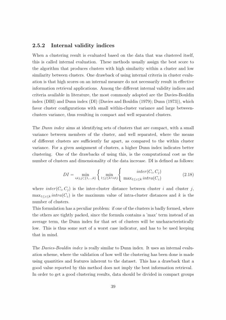
2.5.2 Internal validity indices
When a clustering result is evaluated based on the data that was clustered itself,
this is called internal evaluation. These methods usually assign the best score to
the algorithm that produces clusters with high similarity within a cluster and low
similarity between clusters. One drawback of using internal criteria in cluster evalu-
ation is that high scores on an internal measure do not necessarily result in effective
information retrieval applications. Among the different internal validity indices and
criteria available in literature, the most commonly adopted are the Davies-Bouldin
index (DBI) and Dunn index (DI) (Davies and Bouldin (1979); Dunn (1973)), which
favor cluster configurations with small within-cluster variance and large between-
clusters variance, thus resulting in compact and well separated clusters.
The Dunn index aims at identifying sets of clusters that are compact, with a small
variance between members of the cluster, and well separated, where the means
of different clusters are sufficiently far apart, as compared to the within cluster
variance. For a given assignment of clusters, a higher Dunn index indicates better
clustering. One of the drawbacks of using this, is the computational cost as the
number of clusters and dimensionality of the data increase. DI is defined as follows:
DI = mini 6=j,j⊂{1,...,k}
{min
1≤j≤k∧i 6=j
{inter(Ci, Cj)
max1≤z≤k intra(Cz)(2.18)
where inter(Ci, Cj) is the inter-cluster distance between cluster i and cluster j,
max1≤z≤k intra(Cz) is the maximum value of intra-cluster distances and k is the
number of clusters.
This formulation has a peculiar problem: if one of the clusters is badly formed, where
the others are tightly packed, since the formula contains a ’max’ term instead of an
average term, the Dunn index for that set of clusters will be uncharacteristically
low. This is thus some sort of a worst case indicator, and has to be used keeping
that in mind.
The Davies-Bouldin index is really similar to Dunn index. It uses an internal evalu-
ation scheme, where the validation of how well the clustering has been done is made
using quantities and features inherent to the dataset. This has a drawback that a
good value reported by this method does not imply the best information retrieval.
In order to get a good clustering results, data should be divided in compact groups
39

that show low degree of similarity (this condition can be mathematically expressed
by a high value of S(Ci, Cj), i.e. the distance between centroids of cluster i and the
centroid of cluster j). DBI is defined as follows:
DBI =1
n
n∑i=1
maxi 6=j
{Sn(Ci) + Sn(Cj)
S(Ci, Cj)
}(2.19)
where Sn(Cx) is the average distance of each element of a cluster with respect to
the centroid of cluster Cx (and 1 ≤ x ≤ k) to which they belong, S(Ci, Cj) is the
distance between centroids of cluster i and the centroid of cluster j and k is the
number of clusters. Hence the ratio is small if the clusters are compact and far from
each other. The index is symmetric and non-negative. Due to the way it is defined,
as a function of the ratio of the within cluster scatter, to the between cluster sepa-
ration, a lower value will mean that the clustering is better.
Davies-Bouldin index and Dunn index are the indices used in this work to evaluate
the performance of obtained clustering. This choice is mainly due to the fact that
the optimal configuration (i.e. the optimal number of clusters) for the system under
consideration is not known, so that only internal validity measures can be used. As
already stressed, these indices have the main drawback that good values reported
by these methods do not imply the best information retrieval: to overcome this
limitation the most reasonable solution is a multi-assessment, employing more than
one internal validity measure. Both Davies-Bouldin index and Dunn index are thus
employed in this work, and the choice of the optimal number of clusters is made
according to the values of both indices: in particular the optimal number of clusters
is the one that maximizes the Dunn index and minimizes the Davies-Bouldin index.
40

Chapter 3
The Marina Reservoir case study
The purpose of this chapter is to introduce the case study to which the hybrid
approach that couples DEMo procedure to clustering techniques is applied. In par-
ticular in Section 3.1 and 3.2 the reader is introduced to water management issues in
Singapore and to a general description of Marina Reservoir water system. Then, Sec-
tion 3.3 describes the management problem of the reservoir, while Sections 3.4 and
3.5 give an overview of Marina Reservoir developed modelling tools that constitutes
the basis for the identification of an emulator.
3.1 Water management issues in Singapore
Lying almost on the equator, the Republic of Singapore, the second-smallest country
in Asia, consists of Singapore Island and 63 smaller adjacent islets. It’s situated in
the Indian Ocean off the southern tip of the Malay Peninsula, and has an area of
693 km2. Singapore’s position at the eastern end of the Strait of Malacca, which
separates western Malaysia and the Indonesian island of Sumatra, has given it eco-
nomic and strategic importance out of proportion to its small size. The climate is
tropical, with heavy rainfall and high humidity. The range of temperature is slight:
the average annual maximum is 31 ℃, and the average minimum 24 ℃. The annual
rainfall of 2500 mm is distributed fairly evenly throughout the year, mainly from
December to February. Singapore is facing a serious shortage of water resources. Its
current water demand is about 1.4 million cubic meters daily. Water resource man-
agement becomes, therefore, a strategically important issue for national economic
development and public and social life.
From the 1980s to 1990s Singapore made tremendous efforts in a legal and manage-
41

ment system for the environment (including water), in conducting pollution control,
river cleaning and setting up industrial estates according to land planning, and in
building up a world class urban sanitation system including water and sewerage
networks and treatment plants covering the whole island. From the later 1990s un-
til the present the government has set sustainable water supply as the main target
of water strategy, and for this a series of initiatives and actions have been taken,
and the country has achieved remarkable progress in water resource management.
To achieve this, several ambitious programs are being undertaken. Among this,
the 4 national taps strategy (see Board, 2005 and Bank, 2006) is by far the most
important. The taps are organized as follows:
TAP 1. Catchment Management Watershed conservation is vitally important
to ensure water quality in the reservoirs, especially considering that most of the
catchments are located in urban areas. Because of close coordination between
land use planning and water catchment activities, water catchment accounted
for about 50% of the land area of Singapore. After the creation of Marina
barrage, the increase in the supply of water was about 10 % of current water
needs, and the effective catchment area in Singapore increased to two thirds
of the total land area.
TAP 2. Imported water Singapore imports its entitlement of water from the
neighbouring Johor state of Malaysia, under long-term agreements signed in
1961 and 1962, when Singapore was still a self-governing British colony. Under
these agreements, Singapore can transfer water from Johor for a price of less
than 1 cent per 1,000 gallons until the years 2011 and 2061 respectively. The
water from Johor is imported through three large pipelines across the 2-km
course way that separates the two countries. Singapore would like to ensure
its long-term water security by having a treaty which will provide it with
the stipulated quantity of water well beyond the year 2061. In contrast, the
main Malaysian demand has been for a much higher price of water, which
has varied from 15 to 20 times the present price. That’s why the target of
Singapore government is increasing the portions of the first, third and fourth
Taps.
TAP 3. NEWater program The PUB started to test the production of NEWater
(treated waste-water) in 1998. The treated waste-water becomes a new water
resource, which closes the water loop. The NEWater application in Singapore
42

is the largest in non-potable waste-water reuse in the world, and marks a
milestone in the development of water reuse. The target was to supply 250,000
m3/day of NEWater for direct non-potable use, or 15% of the Singapore water
supply, by the year 2011. To launch such a potentially controversial product
due to the nature of its source, and make it acceptable by Singaporeans in such
a short span of time requires a careful plan, and a well-timed and properly
coordinated public communications strategy.
TAP 4. Desalinated water The first desalination plant using reverse osmosis
(RO) technology and with a capacity 136,380 m3/day was commissioned in
September 2005. This seawater plant is one of the first and largest of such
facilities in the region.
3.2 Marina Reservoir water system
Among these taps, the maximization of water yields from local catchments is poten-
tially one of the most important sources, and with the inclusion of Marina Reservoir
the Singapore’s effective catchment area is now increased to about 50% of the total
available area. Marina Reservoir, which was created in late 2008 with the construc-
tion of a 350 m wide barrage across Marina Channel, represents one of the largest
fresh water bodies in Singapore. Besides this strategic water supply role, the reser-
voir has two further functions: floods control and lifestyle attraction. Indeed, the
Marina Bay area coincides with most of Singapore’s Central Region and it has been
the site around which an ambitious urban development project took place.
The reservoir has a surface area of 2.45 km2 and an active storage of about 3.2 hm3.
Five main tributaries (Singapore, Geylang and Kallang river and Bukit Timah and
Stamford Canal) discharge water into the reservoir draining a catchment of approx-
imately 100 km2, about 1/7 of Singapore total surface area, that produces a mean
annual inflow of about 150 hm3 with a typical tropical pattern.
The catchment mainly consists of urbanized land and it is characterized by the
presence of three further reservoirs, only managed for drinking water supply and
whose discharge to Marina Reservoir is rare and negligible. The weather conditions
are mainly driven by the monsoon seasons, but with no distinct wet or dry peri-
ods, as rainfall events can occur during every month of the year (Selvalingam et al.,
1987). The North-East monsoon occurring from November to February/March is
the wettest season with strong rainfalls coming from the South China Sea, while
43

MarinaReservoir
MALAYSIA
INDONESIA
SINGAPORE
SingaporeStrait
(a) Marina Reservoir and its catchment
(b) Overview of the Barrage and the visitor center where pumps
are located
Figure 3.1: The Marina Reservoir water system.
44

the South-West monsoon from June to September is less intense. During the inter-
monsoon seasons Sumatra squall lines, coming from the westward Indonesian Suma-
tra Island, usually shower Singapore on early mornings. Moreover, added to this
large scale pattern, convection enhanced by the warm water pool surrounding the
island, the high relative humidity of the atmosphere and the hot spots of heat espe-
cially spread in the urban areas, bring heavy rainfall events associated with strong
and relatively-fast thunderstorms of about 2-3 hours.
The drainage system consists of concrete lined canals, thus making the concentra-
tion time of the catchment extremely short (about two hours). Rainfall tends to
come in high intensity events and discharges occur in high peaks over short periods,
typically a few hours. Base flow is low and the upstream canals are mostly dry. In
the downstream parts of the drainage system the bottom level of the canals is often
lower than the reservoir level, with stagnant water being present during draught
periods (Liew et al., 2001). Its peculiar location makes water quality control a rel-
evant issue: the inflow is characterized by short bursts of high flow with sediment
and nutrient rich water followed by dry periods with almost no flow, and because
of its location in the tropics temperature and light intensity are high (as shown in
Antenucci et al., 2012 and Smits and J.V., 2007b). This typically leads to eutrophic
in-reservoir water conditions.
However, satisfying this operational target is not straightforward, mainly because
of the extremely short concentration time of the catchment that causes high peaks
of discharge over a period of few hours (Janssen and Ogink, 2007). Moreover, the
relatively recent formation of the impoundments from a former estuary and the
presence of salinity intrusion make salinity control another important objective.
3.3 Motivation
The efficient management of Marina Reservoir calls for the adoption of novel tools,
capable of accounting for the aforementioned water quantity and quality targets in a
fast-varying hydro-meteorological system. In particular, this management problem
requires a research activity in both a modelling and control domain: in fact the
physically-based models traditionally adopted to describe the ecological conditions
of water reservoirs cannot be employed for optimal decision-making purposes, since
their computational requirements does not allow for their integration with optimiza-
tion framework.
45
This problem can be addressed by resorting to emulation techniques (see Chapter 1),
which allow identifying a simple and computationally efficient copy of the original
model to be used for optimization purposes.
As far as the control domain is concerned, one possible solution is adopting a real-
time control approach that can exploit the availability of hydrological information
(e.g. precipitation and runoff forecasts) thus enhancing the efficiency of the man-
agement system. The proposed management system to be developed is thus a com-
bination of emulators with real-time control techniques.
In the context of Marina Reservoir it must be understood that an operational
management system is already in place (Twigt and Burger, 2010): the barrage
is equipped with 9 surface gates, 7 pumps (to discharge water when the sea level is
higher than the reservoir one, with an installed capacity of 280 m3/s ) and 2 bottom
pipes, which can release water at deeper levels, thus allowing for the mechanical
control of the temperature profile and the salinity concentration. This tools are not
sufficient because also water quality objectives have to be taken into account in the
real-time control of the water system.
Actually, there is a model available for the water system but this is computationally
too intensive to be used for real time control. An effective approach to overcome
this limitation is to perform a top-down reduction of the physically-based mode
describing the hydro-dynamics of Marina Reservoir by identifying a simplified, com-
putationally efficient emulator, constructed from, and then used in place of the
original process-based model in highly resource-demanding tasks, like the optimal
management of the reservoir.
Next section gives an overview of Marina Reservoir developed modelling tools that
constitute the basis for the identification of the above-mentioned emulator.
3.4 Description of the models available
For Marina Reservoir, an extensive modelling framework is available for simulation
and forecasting (Twigt and Burger, 2010). These models are also integrated into
the operational management system. Different components of the water system are
modelled by different modules that can either run independently or coupled from
each other. The modules are:
- rainfall-runoff and 1D flow module that calculates the runoff from the different
sub-catchments and the water flow through the drainage system;
46

1D FLOW
RR RTC
Delft3DFLOW
Figure 3.2: Flow diagram of simulation model.
- 3D flow that calculates the hydrodynamics of Marina reservoir;
- real-time control module that applies the control of structures in the model
depending on the simulation results.
All the different modules are integrated in a 1D-3D coupled model, whose architec-
ture is shown in Figure 3.2, where RR and RTC stand for rainfall-runoff module
and real-time control module. Its operation is as follows: the rainfall runoff module
runs independently first. This provides boundary conditions for the 1D and 3D flow
modules. These two modules run together with the RTC module. The 1D flow and
3D flow coordinates discharge and water level at their combined boundary. The
RTC module sets the states of controllable structures (gates and pumps of the ma-
rina barrage) depending on the state in the system. Currently there is a fixed set
of operating rules that is implemented by this module. There is also an emission
module that calculate the loads of constituents at the rainfall runoff boundary after
which the 1D and 3D water quality modules calculates the transport of and the
processes associated with the constituents. As these modules are not used in this
work, the reader is referred to Smits and J.V. (2007a) and Smits and J.V. (2007b)
for further details.
47

All the models are built using the commercial software packages Sobek (Deltares,
2010) and Delft3D (Deltares, 2010) that are developed by Deltares. In the follow-
ing paragraph a short overview of the modelling concepts is given for each module.
For a more detailed description the reader is referred to the available documentation
about the model development and the user guides of the Sobek and Delft3D software
packages.
3.4.1 Rainfall-runoff and 1D flow module
The hydrology is described in the rainfall-runoff module Sobek RR and the hy-
draulics is described in a combined application of the Channel Flow and Sewer Flow
modules Sobek CF/SF (see Zijl and Twigt, 2007 for further details). The input
for the model consisted of a MIKE11 model of the catchment as provided by PUB
(Public Utilities Board).
Since it is not possible to include all small drains in the schematization of the model,
the catchment has been divided into 196 sub-catchments for which a general schema-
tization is applied. In each of these sub-catchments the rainfall-runoff process and
the drainage to the main channels is described using the following two network el-
ements: manholes and pipes. The manhole stores the total runoff (or acts as a
collection point for the runoff) and the pipe conveys the stored runoff to the main
channel.
The Sobek schematization has been extended with artificial manholes used in the
rainfall-runoff module, and pipes connecting the manholes to the channel flow sys-
tem. Various adjustments to the schematization have been made. Rainfall stations
of PUB and NEA are assigned to rainfall-runoff manhole nodes to get the rainfall
data. The assignment is based on Thiessen polygons. For this hourly rainfall data
is used. Evaporation is set to a constant value of 3.23 mm/day (Singapore mean
daily evaporation).
The calculation was not done at every cross-section, but with a 1D discretization of
the Saint-Venant equations. Sobek uses a staggered grid discretization (with a res-
olution of 100 m) in which the water level is calculated in nodes and the discharge
between nodes. This choice makes the model much faster (reduces computation
times by a factor of four). The rainfall-runoff module and channel flow module are
run sequentially. The results of the Sobek model are used as input to the Delft3D
model.
48
3.4.2 3D flow module
The 3D hydrodynamic models (see Zijl and Twigt, 2007 for further details) used to
calculate the flow condition in Marina Reservoir have been developed as applications
of Delft3D. At the core of Delft3D is the FLOW module (Deltares, 2010) for the
simulation of water flow in three dimensions. The three-dimensional hydrodynamic
model equations that form the basis of FLOW are written in a generalised orthogonal
coordinate system. Depending on the size and complexity of the problem and model
domain, a choice between a rectangular model grid, a curvilinear or a curvilinear
spherical model grid in the horizontal can be made. The non-linear equations are
discretized using a finite difference discretization and are solved by an efficient, stable
and accurate ADI-type solution technique. For complex geometries such as Marina
Bay, a curvilinear grid allows for maximal boundary fitting, that is to say best grid
representation of the curved contours of shores.
The horizontal model grid of the 3D Marina Reservoir model covers the Marina
Bay basin, Kallang basin and Marina Channel. Furthermore it extends up to 2
km upstream into Kallang River, Rochor Channel, Geylang River, Singapore River
and Stamford Canal. This is done because stratification can be expected in those
areas. The areas of the Marina Bay basin, Kallang basin and Marina Channel have
a grid size of 25 m by 25 m. Further upstream larger grid cells have been used, with
grid sizes (in the direction along the river) of more than 100 m. By varying the
grid sizes, computational time is saved, while correctly representing relevant local
spatial scales. Figure 3.3 shows Delft3D bathymetry. By shutting off Marina Bay
from the tide coming from Singapore Straits, Marina Reservoir can be characterised
as weekly-dynamic system presumably with temporary stratified areas. Therefore,
the z-layer approach for the vertical schematization is used. This implies that strictly
horizontal computational layers are defined, with a user-defined thickness.
In the 3D Marina Reservoir model a maximum of 12 computational layers (in the
deepest parts) is used. The layer thickness varies over the vertical. The thinnest
layer can be found at the water surface, gradually increasing towards the bottom.
The vertical schematization has been decided after a number of sensitivity tests.
With Delft3D it is possible to make an on-line coupling with a Sobek model. This
can be useful when a model is required that covers extensive river branches as well as
basins or estuaries where 3D effects (e.g. stratification) play a significant role. There
are 33 boundaries at which the 3D model connects with the 1D network: 30 inflow
points (29 surface flow and one groundwater flow), weirs, pumps and pipes. Both
49

Figure 3.3: Delft3D bathymetry.
systems simulate time dependent processes for which a time stepping procedure is
applied. In the coupled 1D-3D hydrodynamic model quantities are exchanged at
each time step. As an explicit coupling is applied, every time step Sobek sends
discharge values to Delft3D and Delft3D sends water level data to Sobek.
Consequently, there is a time step restriction. The exchange of data is done every
time step of the 1D model, that corresponds with each half time step of the 3D
model because of the specific alternate direction implicit method that is used to
solve the 3D equations.
3.4.3 Operating rules of barrage
The barrage consists of 9 gates, 2 bottom pipes and seven pumps. The maximum
allowed reservoir water level is 1.1 m. However, the goal of the operation rules for
the weirs (gates), pipes and pumps at the barrier is to keep the water level in Marina
Reservoir between -0.2 (-0.3) and +0.3 m (i.e. levels between 99.8 m and 100.3 m
in Singapore Datum) as often as possible.
The pipes and weirs are used to discharge water during low tide periods, when the
sea water level is at least 20 cm below the reservoir water level.
All weirs are opened when the water level is greater than 1.0 m and outside water
level is at least 20 cm lower. All pumps are switched on during high tide periods
when the reservoir water level greater than 0.7 m. However, gates, pipes and pumps
50

are operated according to fixed operating rules, that are briefly described in (Smits
and J.V., 2007a).
3.5 DEMo problem conceptualization
As anticipated, the efficient management of Marina Reservoir should be capable of
accounting for water quantity and quality targets: this calls for the adoption of novel
tools in a fast-varying hydro-meteorological system. Delft3D cannot be employed
for optimal decision-making purposes, since its computational requirements does not
allow for its integration with optimization framework.
This problem can be solved by means of the emulation techniques, which allow iden-
tifying a simple and computationally efficient surrogate of Delft3D to be used for
the optimization purposes introduced in Section 3.3. Before applying any DEMo
technique to Delft3D, a pre-processing of the exogenous drivers, controls, and state
variables to reduce the high number of variables appearing in the final emulator is
required.
This operation can be either performed in different ways: with the purpose of pre-
serving the physical interpretation of the aggregated state variables, while develop-
ing an automatic and system-independent tool, Chapter 4 of this thesis explores the
potential of cluster techniques to discover compact and relevant representations of
high-dimensional data sets produced via simulation of Delft3D.
The identified clusters are then processed with a Recursive Variable Selection algo-
rithm, in order to single out the most relevant clusters of some specific state variable
that are relevant to the emulator’s output, which, in this case, is the salinity con-
centration in a point close to the barrage. The rationale behind this choice is that
in this point the salinity concentration trajectories assume the highest values with
respect to all the other areas within the reservoir. These high values are in fact
not consistent with the high daily demand of fresh water, coupled with the serious
shortage of water that Singapore is nowadays facing. The presence of the desali-
nation plant from 2005 is not sufficient to ensure the necessary water supply, and
an optimal management of the reservoir should take into account a reduction of the
salinity concentration of the water sent to the plant itself. Moreover a lower level
of salinity would guarantee better in-reservoir water quality conditions for aquatic
animals and plants.
51


Chapter 4
DEMo by hierarchical clustering
The scope of this emulation modelling exercise is to reduce the dimensionality of
Delft3D so that the emulation model can be used to design, via the resolution of
a management problem, the optimal control policy for the gates, pipes and pumps
being employed to reduce the water quantity and quality problems affecting the
reservoir. In particular, this work concerns the management of salinity concentration
in the reservoir itself. The chapter is organized as follows: Section 4.1 describes the
Design of computer experiments and simulation runs phases, while Section 4.2 is
mainly concerned with variable aggregation, which is the core of this work. In
Section 4.3 variable selection is performed and in Section 4.4 the emulation model
is identified. Section 4.5 finally shows a comparison of hierarchical clustering results
with the results of another simpler aggregation method applied to the same data-
set, in order to stress the potential of a completely automatic aggregation procedure
with respect to an expert-skills based one.
4.1 DOE and simulation runs
The final scope of DOE is to explore, via simulation of the physically-based model,
the largest possible area within the LYt×LWt×Lut and LXt×LWt×Lut spaces (where,
in particular, LWt is the space of drivers, Lut is the space of controls, LYt is the
space of the output to be explained, and LXt is the space of the states). To this pur-
pose, for each simulation run, it is necessary to specify a trajectory over the whole
simulation horizon H for all the physically-based model input variables, namely the
exogenous driver Wt and the control ut.
To calculate the flow conditions in Marina Reservoir the 3D model Delft3D was
53

Variable Description Units
It surface inflow m3/s
GIt groundwater inflow m3/s
CCt fraction of cloud coverage %
RHt relative humidity %
ATt air temperature °CWSt wind speed m/s
WDt wind direction deg
Table 4.1: Components of exogenous driver vector Wt.
Variable Description Units
u1t release from gates m3/s
u2t release from pipes m3/s
u3t release from pumps m3/s
Table 4.2: Components of control vector ut.
adopted. The Delft3D exogenous driver Wt includes 7 components accounting for
the main hydro-meteorological processes (i.e. surface inflow, groundwater inflow,
fraction of cloud coverage, relative humidity, air temperature, wind speed, and wind
direction), while the control vector ut has three components, i.e. the release from
gates, pipes and pumps (see Tables 4.1 and 4.2).
The model has 7 state variables (salinity concentration, temperature, salinity and
temperature transport1, u-direction velocity, v-direction velocity, and w-direction
velocity) for each computational cell, hence considering a total of 111 observation
points and 12 computational layers, the state vector Xt (see Table 4.3) has a total
of nearly 104 variables. Also water level in each observation point is examined. The
real-to-run time ratio associated to this set-up is of about 1:100. With the purpose
of generating the data-set of samples F , a set of trajectories for the model inputs
Wt and ut is designed.
1Dimensionless coefficients. Notice that the transport of matter (salinity in this case) and heat
is modelled by an advection-diffusion equation in the three coordinate directions.
54

Variable Description Units
salit salinity ppt
tempit temperature °CST i
t salinity transport %
TT it temperature transport %
UV it u-velocity m/s
V V it v-velocity m/s
WV it w-velocity m/s
Table 4.3: Summary of Delft3D state variables Xt notation (computed for each i cell of the spatial
domain).
As for the exogenous driver Wt, the time-series of observational data over the period
April 2009 - April 2010 is available, while, concerning ut, 10 different management
scenarios are generated, for a total of 10 simulation scenarios.
- Scenario 1 In this simulation pipes are always used when it’s possible;
- Scenario 2 In this simulation pipes are not used;
- Scenario 3 In this simulation pumps are not used;
- Scenario 4 In this simulation only gates are used;
- Scenario 5-10 The difference among the simulations stands in the way in
which the controls are managed or simply in the decision of employing all or
only some control devices.
The target of the emulation modelling exercise is to reduce as much as possible the
number of state variables involved in the physically-based model concerning salinity
concentration in the reservoir. Thus, the output Yt is the salinity concentration
[ppt] in the deepest point of the reservoir, located few hundred meters from the
barrage, where the effect of salinity is stronger (see Figure 4.1 for its localization in
the bathymetry); the output is therefore characterized by a dimensionality equal to
1, with an hourly time-step.
All the simulations are run with 30 sec simulation time-step, and an average vertical
resolution of about 0.5 m. The data are sampled with an hourly time-step, and
finally stored in a data-set F of ∼ 8 · 104 tuples.
55

Figure 4.1: Localization of the point used in the elaborations.
4.2 Variable aggregation by time-series clustering
The spatially-distributed nature of Delft3D model leads to a large dimensionality
of the state and exogenous driver vectors. By processing the data in F with a
suitable aggregation scheme, Xt and Wt are transformed in two lower-dimension
vectors Xt and Wt, so that the majority of the variation in the original vectors is
captured. The aggregation scheme can be done in different ways: with the purpose
of preserving the physical interpretation of the aggregated state variables, while
developing an automatic and system-independent tool, this section explores the po-
tential of clustering techniques to discover compact and relevant representations
of high-dimensional data sets. The rationale behind this choice is that clustering,
by organizing data into homogeneous groups with minimized within-group-object
similarity and maximized between-group-object dissimilarity (Liao, 2005), can be
effective in providing a compact, yet informative, representation of the data pro-
duced with the Delft3D, thus enhancing the final emulator accuracy and reducing
the computational and analytical effort of the DEMo process. Unlike static prob-
lems, the data here considered are a set of time-series with a spatial distribution.
This implies the adoption of time-series clustering techniques that aims at deter-
mining groups of similar time-series.
56

The hierarchical agglomerative cluster algorithm (Magni et al., 2008) is the selected
method: it works by organizing the data (the time-series) into a tree of clusters.
In the present configuration, the distance between each cluster is measured as Eu-
clidean distance, while clusters are merged according to the Ward’s minimum vari-
ance method (at each clustering step, the merge that minimizes the increase in the
sum-of-squares variance is chosen). The Ward’s method minimizes the total within-
cluster variance, and thus goes in the desired direction of creating compact and
informative clusters, which can then be processed with the RVS-IIS algorithm.
Eventually, the choice of the optimal number p of clusters for each state variable is
chosen according to the Davies-Bouldin (DBI) and Dunn (DI) index (Davies and
Bouldin, 1979; Dunn, 1973), which favour cluster configurations with small within-
cluster variance and large between-clusters variance, thus resulting in compact and
well separated clusters.
Next sections examine in detail the selected clustering algorithm and show the pri-
mary positive aspects of the chosen distance measure, linkage method, and clustering
evaluation criteria.
Hierarchical clustering
In this work, hierarchical clustering method is adopted. Hierarchical clustering tech-
niques (Magni et al., 2008) are the second important category of clustering methods.
As with K-means, these approaches are relatively old compared to many clustering
algorithms, but they still enjoy widespread use: in particular, agglomerative hier-
archical clustering techniques are by far the most common. Hierarchical clustering
algorithm applied on time-series data works by organizing the time-series into a tree
of clusters. At the first iteration the algorithm places each time-series in its own
cluster and then starts to merge these small clusters, until a single cluster is obtained
or an a-priori defined stopping condition is satisfied (e.g. the minimum number of
clusters). In order to perform hierarchical clustering, TimeClust software package
is used (see Figure 4.2).
Euclidean distance
Agglomerative clustering methods uses the dissimilarities (similarities) or distances
between objects when forming the clusters. Similarities are a set of rules that serve as
57

Figure 4.2: Time Clust input screen example.
criteria for grouping or separating items. These distances (similarities) can be based
on a single dimension or multiple dimensions, with each dimension representing a
rule or condition for grouping objects. In the present configuration, the distance
between each cluster is measured as Euclidean distance, that is computed as shown
in equation 2.8. One reason is that the centroid or the ward algorithms should
be used only with the euclidean distance; moreover, this distance measure is not
affected by the presence of outliers.
Ward linkage method
At the first step, when each object represents its own cluster, the distances be-
tween the objects are defined by the chosen distance measure. However a linkage
or amalgamation rule to determine when two clusters are sufficiently similar to be
linked together is needed. There are numerous linkage rules such as these that have
been proposed in Section 2.4: in this thesis, clusters are merged according to the
Ward’s method (at each clustering step, the merge that minimizes the increase in
the sum-of-squares variance is chosen). The Ward’s method considers the union
of every possible pair of clusters and combines the two clusters whose combination
results in the smallest increase in ESS (Total Error Sum of Squared deviations from
the cluster centroid), and thus goes in the desired direction of creating compact and
58
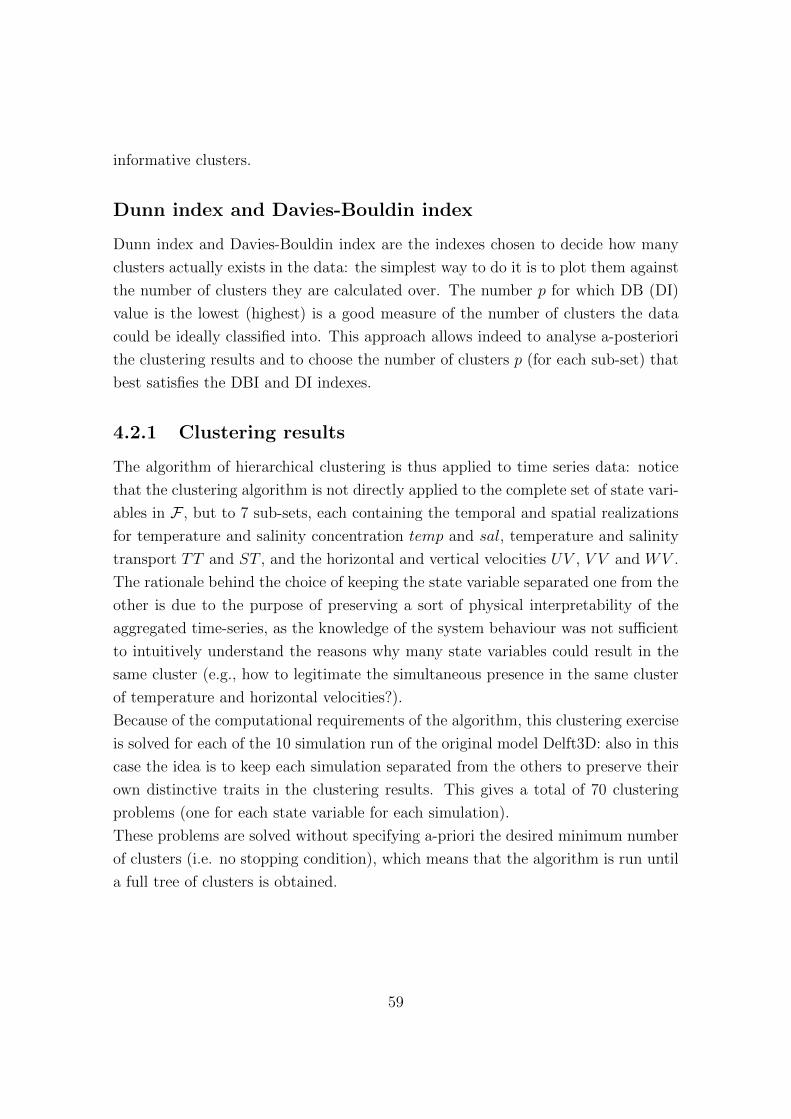
informative clusters.
Dunn index and Davies-Bouldin index
Dunn index and Davies-Bouldin index are the indexes chosen to decide how many
clusters actually exists in the data: the simplest way to do it is to plot them against
the number of clusters they are calculated over. The number p for which DB (DI)
value is the lowest (highest) is a good measure of the number of clusters the data
could be ideally classified into. This approach allows indeed to analyse a-posteriori
the clustering results and to choose the number of clusters p (for each sub-set) that
best satisfies the DBI and DI indexes.
4.2.1 Clustering results
The algorithm of hierarchical clustering is thus applied to time series data: notice
that the clustering algorithm is not directly applied to the complete set of state vari-
ables in F , but to 7 sub-sets, each containing the temporal and spatial realizations
for temperature and salinity concentration temp and sal, temperature and salinity
transport TT and ST , and the horizontal and vertical velocities UV , V V and WV .
The rationale behind the choice of keeping the state variable separated one from the
other is due to the purpose of preserving a sort of physical interpretability of the
aggregated time-series, as the knowledge of the system behaviour was not sufficient
to intuitively understand the reasons why many state variables could result in the
same cluster (e.g., how to legitimate the simultaneous presence in the same cluster
of temperature and horizontal velocities?).
Because of the computational requirements of the algorithm, this clustering exercise
is solved for each of the 10 simulation run of the original model Delft3D: also in this
case the idea is to keep each simulation separated from the others to preserve their
own distinctive traits in the clustering results. This gives a total of 70 clustering
problems (one for each state variable for each simulation).
These problems are solved without specifying a-priori the desired minimum number
of clusters (i.e. no stopping condition), which means that the algorithm is run until
a full tree of clusters is obtained.
59

0 2 4 6 8 10 120.2
0.3
0.4
0.5
0.6Temperature transport
# cluster
DB
I
0 2 4 6 8 10 120
0.2
0.4
0.6
0.8
# cluster
DI
Figure 4.3: Average value (over the 10 simulation runs) of the DBI and DI indexes for the tem-
perature transport TT .
Figure 4.3 reports the average value (over the 10 simulation runs) of the DBI and DI
indexes as a function of p for the temperature transport TT . Results show that the
best number p∗ of clusters that minimizes the DBI and maximizes the DI index is 3,
while the introduction of a larger number of clusters does not improve the clustering
results any further. The plots of the DBI and DI indexes as a function of p for the
other state variables are reported in Appendix A.
This analysis is performed for a maximum value of p equal to 11 corresponding to
the number of layers (a part from the surface layer) in the original model. This
value provides an empirical upper bound to p, since the data could be for example
aggregated by considering the spatial average of each sub-set in the original model
vertical layers (see Section 4.5.1).
The final results obtained for the remaining sub-sets are reported in Table 4.4, where
60

Table 4.4: Selected number of clusters for the different sub-sets composing the vector Xt. The
symbols are explained in Table 4.3.
State Variable sal temp ST TT UV V V WV h
Number of clusters 6 6 4 3 4 6 8 10
the results obtained for the water level h are also shown. The time series algorithm
found a total of 8 different clusterings, each one identifying a set of homogeneous
areas of a particular variable. These areas can vary from sub-set to sub-set, so, for
example, the salinity concentration sal can be grouped into 6 different areas, while
the vertical velocity WV into 8.
In the following sections a more detailed description of clustering results for each
state variable is given.
Salinity
The number of homogeneous areas identified for salinity is 6. As Figure 4.4 shows,
Cluster 1 and Cluster 2 contain the points closer to the barrage. Points in the
middle of Marina channel and in correspondence of the upper part of the reservoir
(i.e. near Kallang River and Geylang River) are in Cluster 4, Cluster 5 and Cluster
6. Table B.1 shows the number of points per layer belonging to each cluster. Cluster
1, Cluster 4, and Cluster 5 contain points in the deepest layers (i.e. from Layer 1
to Layer 5), while points in Layers 6 and 7 are in Cluster 3. Cluster 6 is the biggest
and contains all the points belonging to the upper layers. The number of points per
cluster is not homogeneous: Cluster 2 and Cluster 4, for example, are made up of
only 2 and 4 points, while Cluster 6 contain more than 300 points.
Salinity transport
The number of homogeneous areas identified for salinity transport is 4. As Figure
4.5 shows, Cluster 4 contain points belonging to all the areas of the reservoir, except
the upper part. Points in correspondence of the upper part of the reservoir (i.e. near
Kallang River and Geylang River) are in fact in Cluster 1, Cluster 2 and Cluster
3. Considering how clusters are composed from the point of view of the depth (see
Table B.2) it is possible to notice that Cluster 1 and Cluster 2 mainly contain points
of Layers 7-11, while Cluster 3 contains points belonging only to Layer 10 and 11.
61

Figure 4.4: The 6 clusters identified for the salinity concentration.
Salinity
Cluster 1 Cluster 2 Cluster 3 Cluster 4 Cluster 5 Cluster 6
Layer 1 8 0 0 0 0 0
Layer 2 14 0 0 4 4 0
Layer 3 0 0 0 0 48 0
Layer 4 0 0 0 0 59 0
Layer 5 0 0 5 0 66 0
Layer 6 0 0 79 0 0 1
Layer 7 0 0 81 0 0 4
Layer 8 0 2 0 0 0 96
Layer 9 0 0 0 0 0 108
Layer 10 0 0 0 0 0 111
Layer 11 0 0 0 0 0 111
Table 4.5: Number of points per layer per cluster for salinity (sal).
Cluster 4 is the biggest and contains all the points belonging to all the layers. The
number of points per cluster is not homogeneous: Cluster 3 is made up of only 2
points, while Cluster 4 contain more than 500 points.
62

Figure 4.5: The 4 clusters identified for the salinity transport.
Temperature
The number of homogeneous areas identified for temperature is 6. As Figure 4.6
shows, Cluster 1 contains points belonging to the area near the inlet of Bukit Timah
canal, while Cluster 2 is made up of points located near the inlet of Stamford Canal.
Cluster 6 contains points belonging to Marina Channel and the ones next to the
barrage, and Cluster 5 the points near Geylang River and the ones near the inlet of
Stanford Canal. Table B.3 shows that Cluster 1, Cluster 2, and Cluster 3 contain
points in the middle layers (i.e. from Layer 5 to Layer 7), while points in Layers 2,
3, and 4 are in Cluster 5. Cluster 6 is the biggest and contains points belonging to
all the layers, including the ones in Layer 1. Cluster 2 and Cluster 6 are the biggest
compared to all the others that contain less than 100 points.
Temperature transport
The number of homogeneous areas identified for temperature transport is 3. As
Figure 4.7 shows, Cluster 1 and Cluster 2 contain points belonging to the upper
part of the reservoir (i.e. Kallang River). All the other points are in Cluster 3.
Considering how clusters are composed from the point of view of the depth (see
Table B.4), Cluster 1 and Cluster 2 mainly contain points of the middle and upper
63

Figure 4.6: The 6 clusters identified for the temperature.
Layers (i.e. from 6 to 11), while Cluster 3 contains points belonging only to all the
layers. Cluster 1 and Cluster 2 are really small and contain respectively 1 and 5
points.
Figure 4.7: The 3 clusters identified for the temperature transport.
64
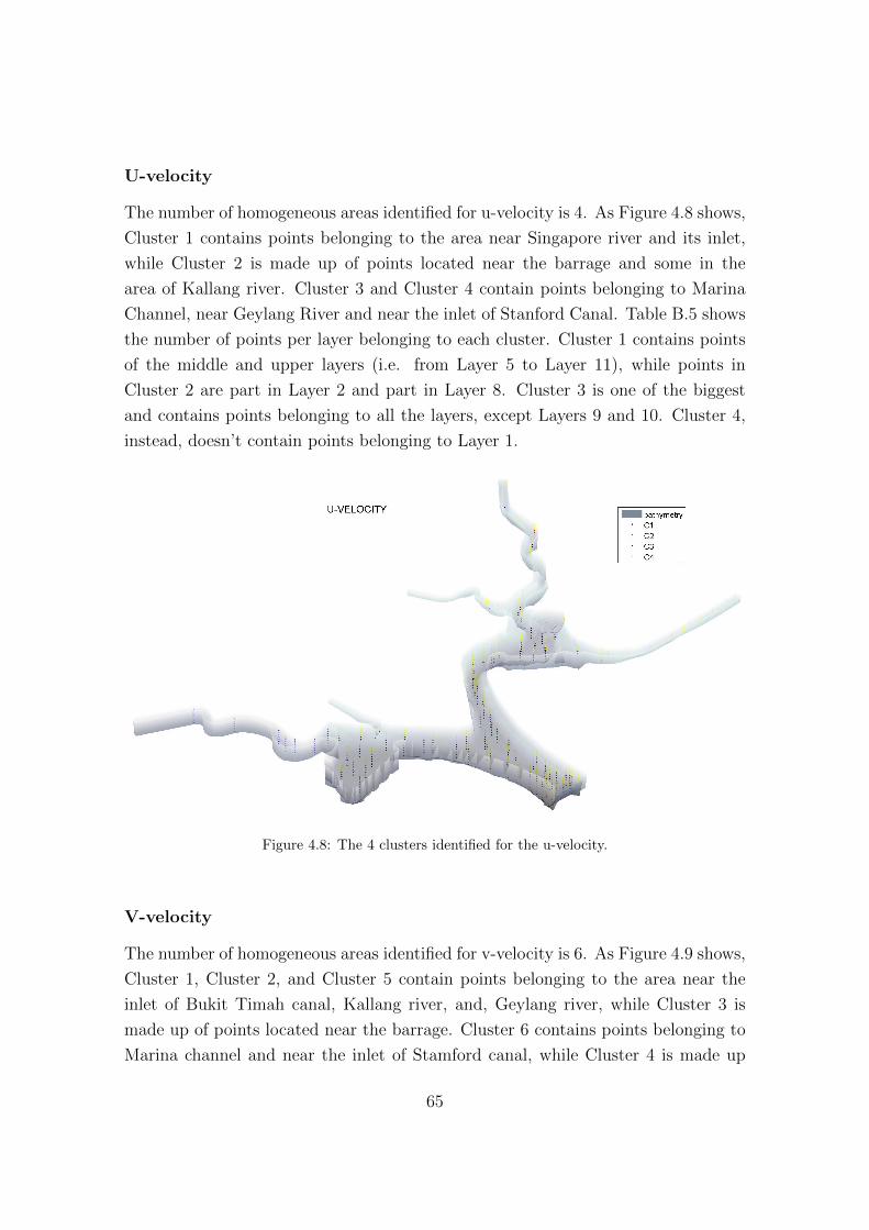
U-velocity
The number of homogeneous areas identified for u-velocity is 4. As Figure 4.8 shows,
Cluster 1 contains points belonging to the area near Singapore river and its inlet,
while Cluster 2 is made up of points located near the barrage and some in the
area of Kallang river. Cluster 3 and Cluster 4 contain points belonging to Marina
Channel, near Geylang River and near the inlet of Stanford Canal. Table B.5 shows
the number of points per layer belonging to each cluster. Cluster 1 contains points
of the middle and upper layers (i.e. from Layer 5 to Layer 11), while points in
Cluster 2 are part in Layer 2 and part in Layer 8. Cluster 3 is one of the biggest
and contains points belonging to all the layers, except Layers 9 and 10. Cluster 4,
instead, doesn’t contain points belonging to Layer 1.
Figure 4.8: The 4 clusters identified for the u-velocity.
V-velocity
The number of homogeneous areas identified for v-velocity is 6. As Figure 4.9 shows,
Cluster 1, Cluster 2, and Cluster 5 contain points belonging to the area near the
inlet of Bukit Timah canal, Kallang river, and, Geylang river, while Cluster 3 is
made up of points located near the barrage. Cluster 6 contains points belonging to
Marina channel and near the inlet of Stamford canal, while Cluster 4 is made up
65

of points located on Kallang river. Table B.6, instead, shows that Cluster 1 and
Cluster 5 contain points of Layer 10 and 11, while Cluster 2 and Cluster 4 contain
points of the middle and upper layers (i.e. from Layer 4 to Layer 9-10); points of the
lower layers are in Cluster 3. Cluster 6 is the biggest and contains points belonging
to all the layers.
Figure 4.9: The 6 clusters identified for the v-velocity.
W-velocity
The number of homogeneous areas identified for w-velocity is 8. As Figure 4.10
shows, Cluster 1, Cluster 2, Cluster 3, Cluster 4, Cluster 7 and Cluster 8 contain
the points closer to the barrage and in Marina channel. Points near the inlet of
Stamford canal and Singapore river are in Cluster 6. This latter contains also points
of other areas, like the ones near the inlet of Geylang river, Kallang river and Bukit
Timah canal. Some of these points are also in Cluster 5. Looking at Table B.7 it is
possible to notice that Cluster 3 and Cluster 4 contain points in the deepest layers
(i.e. Layer 1 and 2), while Cluster 5, Cluster 7 and Cluster 8 contain points of the
medium and upper layers (i.e. from Layer 5 to Layer 11). Cluster 2 is made up
of points belonging only to Layer 10 and 11. Cluster 6 is the biggest and contains
points of all the layers.
66

Figure 4.10: The 8 clusters identified for the w-velocity.
Water level
The number of homogeneous areas identified for water level is 10. As Figure 4.11
and Table B.4 show, Cluster 1 and Cluster 2 contain points close to Singapore river,
while Cluster 5 is made up of points belonging to Marina channel and the ones closer
to the barrage. Cluster 8 and Cluster 9 contain points near the inlet of Stamford
canal and Cluster 4, Cluster 6, and Cluster 7 the ones near the upper part of the
reservoir (i.e. the inlet of Kallang river, Bukit Timah canal and Geylang river). In
this case there is no difference along the depth, as the water level is calculated as
mean value in each observation point.
As a result of this pre-processing phase, the vectors to be considered in the next
variable selection are Xt, Wt, and ut, with dimensionality Mx, nw, and nu respec-
tively equal to 47 (for details see Table 4.4), 7 and 3.
To these vectors, two more variables were eventually added, i.e. the variable t, which
accounts for the system daily periodicity by taking value in the range [1, 365], and
the variable H, which accounts for the system hourly periodicity by taking value in
the range [1, 24]. This gives a total of 59 candidate variables.
67

Figure 4.11: Te 10 clusters identified for the water level.
4.3 Variable selection
The reduction problem requires to select the variables xt, wt and ut constituting the
arguments of the output transformation function ht(·, ·, ·) and the state transition
function ft(·, ·, ·). In particular, the Recursive Variable Selection-Iterative Input
selection algorithm (RVS-IIS, see Section 1.4.3) proposes to first select the features
relevant to the output variable yt, and to then recursively select all the features
relevant to the states xt+1.
In this application, the output is salbarrt , that represents the salinity concentration
in a point close to the barrage (see Section 3.5). As for the underlying model class
and ranking procedure, the IIS algorithm is here combined with Extra-Trees (see
Castelletti et al. (2012a)), whose parameters are set according to ? indications
and subsequent experiences: the number M of trees in an ensemble is 500 (a good
balance between Extra-Trees accuracy and computational requests), the minimum
cardinality nmin for splitting a node is 2 and the number of alternative cut-directions
K (i.e. the number of candidate variables) changes if considering data aggregated
with hierarchical clustering rather than data aggregated according to vertical layers.
The number p of variables singularly evaluated is 5. The IIS algorithm, whose
tolerance ε is posed equal to 0.02, is run only on a part of the whole data-set, in
68

order to overcome problems connected to loss of time due to the computational
requirements of the model structure.
The performance of the emulator being built is evaluated in terms of the coefficient
of determination R2 (in k-fold cross-validation, with k = 10) between the values of
Yt and yt predicted by the emulator. The coefficient of determination is defined as
follows:
R2 = 1− cov(Qi − Qi)
cov(Qi)(4.1)
where Qi are the observed data and Qi are the measured data.
In this case the number of alternative cut-directions K (i.e. the number of candidate
variables) is 59. The vectors to be considered in this phase are Xt, Wt and ut, with
dimensionality respectively equal to 47, 7 and 3. To these vectors, two more variables
were eventually added, i.e. the variable d, which accounts for the system daily
periodicity, and the variable H, which accounts for the system hourly periodicity.
4.3.1 Salinity in a point close to the barrage salbarrt
The first step of the RVS-IIS algorithm requires to identify which variables, among
Xt, Wt and ut, are relevant to describe the the physically-based model output Yt:
these are the arguments of the emulator output transformation function (see eq.
1.4b) that will be identified in the subsequent step.
The results obtained with Step 0 of RVS-IIS, which ranks the importance of all the
candidate features in explaining salbarrt behaviour and then singularly evaluates the
importance of the first ranked three, are reported in Table 4.6 - Step 0. The Table
shows that the output behaviour is almost totally explained by only one variable,
as confirmed by its score (92.60%, 10% more than in the aggregation by vertical
layers), variance reduction and SISO performance: as a matter of fact the average
salinity concentration in Cluster 1 salC1t provides information about the salinity
concentration at the bottom layer in a homogeneous area very close to the barrage.
The IIS algorithm seems to be robust with respect to information redundancy: only
salinity concentration in Cluster 1 salC1t is selected while salinity concentration in
Cluster 4 salC4t is discarded, mainly because Cluster 1 is closer to the barrage than
Cluster 4. The information content of both the two variables is redundant and it
is thus sufficient to employ just one of them in explaining the output salbarrt . In
69

Table 4.6: Results obtained using RVS-IIS algorithm to select the most relevant variables to explain
salbarrt for data aggregated with hierarchical clustering.
Step 0Output variable salbarrt
Initial variance 71807.4000
Candidate Feature Score % Variance Reduction Performance SISO (R2)
salC1t 92.6011 66466.7000 0.9894
salC4t 5.9314 4257.4100 0.9262
GIt 0.2811 201.7440 0.1461
Step 1Output variable salbarrt - v0tInitial variance 767.59
Candidate Feature Score % Variance reduction Performance SISO (R2)
GIt 37.2627 279.2710 0.3916
VVC3 9.6575 72.3798 0.1898
u2t 4.5759 34.2948 0.0436
WVC1 2.7336 20.4871 0.0757
salC5t 2.5936 19.4384 0.0731
this case groundwater inflow GIt is ranked in position three, with a score equal to
0.2811% and a reduction of variance of 201.7440. At the end of this step, the salC1t
term is selected, since it is characterized by the highest SISO model performance
(0.9894). Step 1 of RVS-IIS, whose results are reported in Table 4.6 - Step 1 shows
that the feature with highest score (37.2627%) is the groundwater inflow GIt, with a
variance reduction of 279.2710. The horizontal velocity V V C3 is ranked in position
two; score and variance reduction are definitely low, compared to GIt ones.
Table 4.7: Selected features and corresponding performance of the MISO models obtained for the
case of salbarrt , for data aggregated with hierarchical clustering. State variables are denoted in
bold.
Iteration Feature selected Performance MISO (R2) ∆R2
1 salC1t 0.9893 -
2 GIt 0.9941 0.0048
70

This means that also in this case only the groundwater inflow GIt is relevant in
explaining the residual r0t+1 and that the selection of this new feature let the MISO
model performance increase, with R2 passing from 0.9893 to 0.9941 (see Table 4.7).
However, the introduction of this new variable into the MISO model lead to an
increase of R2 equal to 0.0048, which is lower than the predefined tolerance (ε is set
to 0.02). At this stage the RVS-IIS is stopped and the only selected feature is the
salinity concentration in Cluster 1 salC1t .
4.3.2 Dynamics of salC1t+1
In the set V isalbarrt
of variables selected at the first call of RVS-IIS algorithm, the
salinity concentration in Cluster 1 salC1t is a state variable and, as such, its dynamic
behaviour must be described through suitable state transition equations. The set
V isalC1
tin the subsequent call of the IIS algorithm is still selected among the compo-
nents of the vectors Xt, Wt and ut.
Table 4.8: Selected features and corresponding performance of the MISO models obtained for the
case of salC1t+1. State variables are denoted in bold.
Iteration Feature selected Performance MISO (R2) ∆R2
1 salC4t 0.7787 -
2 u2t 0.9511 0.1724
3 GIt 0.9771 0.0260
4 u1t 0.9806 0.0035
A list of the selected variables is reported in Table 4.8. It can be noticed that salC4t ,
u2t , and GIt, the salinity concentration in Cluster 4, the release from the pipes
and the groundwater inflow, are features relevant to the dynamics of the salinity
concentration in Cluster 1 salC1t+1. In this case also the release from gates appears
(u1t ) in the selected features, but it is not selected as the MISO model performance
increases only of 0.0035.
4.3.3 Dynamics of salC4t+1
Among the variables selected, the salinity concentration in Cluster 4 salC4t is again
state variable, thus requiring a dynamic description too. The results of the RVS-IIS
71

Table 4.9: Selected features and corresponding performance of the MISO models obtained for the
case of salC4t+1. State variables are denoted in bold.
Iteration Feature selected Performance MISO (R2) ∆R2
1 salC4t 0.8628 -
2 u2t 0.9754 0.1126
3 GIt 0.9850 0.0096
algorithm application to salC4t+1 is reported in Table 4.9. At this stage the recursive
variable selection is over, since no further state variables are selected. The pro-
cess took three calls of the RVS algorithm, to single out the most suitable subset
V isalbarrt
of input variables to explain the system output. In particular, the emulator
is characterized by a state vector xt with 2 components (salinity concentration in
Cluster 1 salC1t+1, and salinity concentration in Cluster 4 salC4
t+1), one component of
the exogenous driver vector (i.e. groundwater inflow GIt), and one component of
the original control vector (i.e. pipe inflow u2t ).
The network of the causal relationships between the selected state variables is
sketched in Figure 4.12.
The reduction phase shows that the emulation model output variable salbarrt can
be explained as a function of one exogenous driver (the groundwater inflow GIt),
and one component of the control vector (the pipe inflow u2t ): even though, the
control u2t does not appear to be strongly relevant as its score, variance reduction
and Performance SISO have always low values compared to other variables. Also
the significance of exogenous drivers is rather limited. Furthermore, the state vari-
ables involved are two (the salinity concentration in Cluster 1 salC1t and the salinity
concentration in Cluster 4 salC4t ).
72

ab
Figure 4.12: Graph representation of the variables interactions involved in the emulator output
transformation function (a) and state transition equation (b), for data aggregated with hierarchical
clustering.
4.4 Identification of the emulation model
The outcome of the variable selection (Step 3) are the variables characterizing the
emulator, as well as the nature of the relationship between these variables and
the output yt. This information can be exploited in Step 4 of the DEMo general
procedure (see Figure 1.1), where the structure of the emulator state transition
equation ft(·) and output transformation function ht(·) is selected and the associated
parameters estimated.
This step simply requires to select an appropriate structure (class of functions) for
the emulator, which can then be calibrated and validated. Considering the good
performances provided by Extra-Trees as underlying model in the variable selection
process, they are adopted with the same setting also in this step.
Table 4.10: Structure and performances (R2 and RMSE in k-fold cross validation) of the MISO
models composing salbarrt (salinity concentration in the point close to the barrage) emulation
model, for data aggregated with hierarchical clustering.
Output variable Input variables R2 RMSE
salbarrt salC1t 0.9838 0.3203 (ppt)
salC1t salC4
t−6, PIt−6, GIt−6 0.9437 0.5862 (ppt)
salC4t salC4
t−6, PIt−6 0.9541 0.4501 (ppt)
73
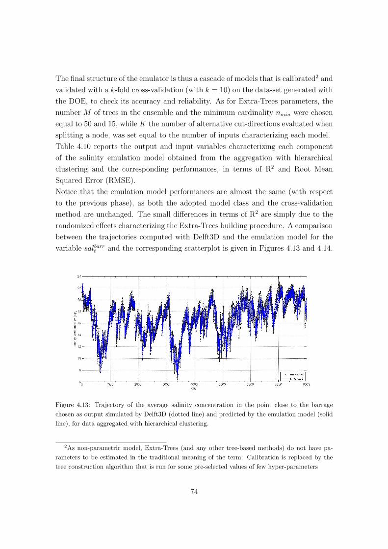
The final structure of the emulator is thus a cascade of models that is calibrated2 and
validated with a k-fold cross-validation (with k = 10) on the data-set generated with
the DOE, to check its accuracy and reliability. As for Extra-Trees parameters, the
number M of trees in the ensemble and the minimum cardinality nmin were chosen
equal to 50 and 15, while K the number of alternative cut-directions evaluated when
splitting a node, was set equal to the number of inputs characterizing each model.
Table 4.10 reports the output and input variables characterizing each component
of the salinity emulation model obtained from the aggregation with hierarchical
clustering and the corresponding performances, in terms of R2 and Root Mean
Squared Error (RMSE).
Notice that the emulation model performances are almost the same (with respect
to the previous phase), as both the adopted model class and the cross-validation
method are unchanged. The small differences in terms of R2 are simply due to the
randomized effects characterizing the Extra-Trees building procedure. A comparison
between the trajectories computed with Delft3D and the emulation model for the
variable salbarrt and the corresponding scatterplot is given in Figures 4.13 and 4.14.
Figure 4.13: Trajectory of the average salinity concentration in the point close to the barrage
chosen as output simulated by Delft3D (dotted line) and predicted by the emulation model (solid
line), for data aggregated with hierarchical clustering.
2As non-parametric model, Extra-Trees (and any other tree-based methods) do not have pa-
rameters to be estimated in the traditional meaning of the term. Calibration is replaced by the
tree construction algorithm that is run for some pre-selected values of few hyper-parameters
74

Figure 4.14: Scatterplot between the trajectory of the average salinity concentration in the point
close to the barrage simulated by Delft3D (y-axis) and predicted by the emulation model (x-axis),
for data aggregated with hierarchical clustering.
Comments
In the previous sections, the procedural, data-driven approach to dynamic emula-
tion modelling combined with hierarchical clustering was applied for the reduction
of Delft3D, a physically-based, hydrodynamic-ecological model describing the dy-
namics of Marina Reservoir (Singapore). The purpose is to achieve a simplified, but
effective, description of salinity concentration dynamics in the deepest layer of an
area very close to the barrage and to solve an optimal control problem concerning
both quantity and quality targets. The reduction part is made by means of hierar-
chical clustering: the clusters obtained turn out to be a compact and informative
representation of the initial larger amount of data available via simulation of the
model itself. The complexity reduction with respect to Delft3D is remarkable, i.e.
from nearly 104 to only 48 variables. The emulation model performances are quite
satisfactory as, despite its simple structure, the emulation model provides good per-
formances.
In particular, the potential of hierarchical clustering performed in this work is that,
despite being an automatic technique, all the selected variables can be given a phys-
ical interpretation: i) the state variables selected provide information about the
salinity concentration in a homogeneous area very close to the barrage; ii) the
groundwater flow represents the main source of the salinity intrusion, while iii) the
75

pipes, located at the bottom of the barrage, have an obvious key role in releasing
water with higher salinity concentrations.
4.5 Choice of a different aggregation method
This section describes the application of DEMo procedure to data grouped with a
different aggregation method: the rationale behind this choice is to show how the
results can vary according to the particular type of aggregation method chosen.
This aggregation method is different from clustering: with the purpose of simply
preserving the physical interpretation of the natural system, in this part of the
work time-series data (referred to each state variable in each simulation) are divided
into groups by assuming that each vertical layer (introduced to take into account the
stratification in Marina Reservoir) can be a sufficiently compact and relevant cluster
well representing a homogeneous area in the high-dimensional data sets produced
via Delft3D simulation runs.
4.5.1 DOE, simulation runs and variable aggregation
The final scope of DOE is to explore, via simulation of the physically-based model,
the largest possible area within the LYt ×LWt ×Lut and LXt ×LWt ×Lut spaces
(where, in particular, LWt is the space of drivers, Lut is the space of controls, LYt is
the space of the output to be explained, and LXt is the space of the states). For each
simulation run, it is thus necessary to specify a trajectory over the whole simulation
horizon H for all the physically-based model input variables, namely the exogenous
driver Wt and the control ut: these vector are unchanged with respect to the case
of data aggregated with hierarchical clustering (see Section 4.1).
As said, in this part of the work time-series data (referred to each state variable in
each simulation) are divided into 12 groups according to the number of vertical layer.
In Table 4.11 the depth of each layer is reported. In such a way 12 groups within the
data are created, in correspondence of the vertical layers. The assumption made is
that data contained in the same layer show a similar behaviour. For the upper layer
(layer 12) data are not always present for each location point at each time step (for
instance, during dry periods), so only the first eleven layers are taken into account
in the subsequent computations. Moreover, the number of points belonging to each
group is not the same because of the bathymetry of the reservoir: for instance, layer
1 contains only 8 points (the points with greater depth), layer 6 contains 80 points,
76

Table 4.11: Depth of each vertical layer in Delft3D stratification.
Layer Depth [m]
Layer 12 0.354 - 1.062
Layer 11 1.062 - 1.753
Layer 10 1.753 - 2.415
Layer 9 2.415 - 3.047
Layer 8 3.047 - 3.653
Layer 7 3.653 - 4.233
Layer 6 4.233 - 4.787
Layer 5 4.787 - 5.318
Layer 4 5.318 - 5.826
Layer 3 5.826 - 6.312
Layer 2 6.312 - 7.050
Layer 1 > 7.050
and layer 11 is made up of 111 points. This difference will affect the next steps
of the procedure, as the average trajectories of each state variable calculated for
layers with a lower number of points are more similar to the trajectories of each
singular point belonging to the layer itself (in this case the cluster well represents
the behaviour of the points that belong to the cluster itself).
Notice that this is only one of the possible aggregations for the time-series data con-
cerning Marina Reservoir. This approach can preserve physical interpretability, but
it requires a number of a-priori assumptions (i.e. the hypothesis that the values of
the state variable measured at the same depth show the same behaviour. In case of
non horizontal homogeneity, vertical stratification cannot be adopted as clustering
criterion) hardly formalizable in a procedural process.
Carry on through DEMo procedure with this approach, the vectors to be considered
in the next phase are Xt, Wt, and ut, with dimensionality Mx, nw and nu respec-
tively equal to 77 (7 state variables for each cluster), 7 and 3. To these vectors,
three more variables were eventually added, i.e. the reservoir level ht, the variable
d, which accounts for the system daily periodicity by taking value in the range [1,
365], and the variable H, which accounts for the system hourly periodicity by taking
value in the range [1, 24]. This gives a total of 90 candidate variables for the variable
selection problem.
77

4.5.2 Variable selection
The reduction problem requires to select the variables xt, wt and ut constituting
the arguments of the output transformation function ht(·, ·, ·) and the state transi-
tion function ft(·, ·, ·). The output is the same: salbarrt , that represents the salinity
concentration in a point close to the barrage. The only difference is that in the
case of data aggregated using vertical layers as aggregation principle, the number of
alternative cut-directions K (i.e. the number of candidate variables) is 90 instead
of 59.
Salinity in a point close to the barrage salbarrt
The first step of the RVS-IIS algorithm requires to identify which variables, among
Xt, Wt and ut, are relevant to describe the the physically-based model output Yt:
these are the arguments of the emulator output transformation function (see eq.
1.4b) that will be identified in the subsequent step.
The results obtained with Step 0 of RVS-IIS, which rank the importance of all the
candidate variables in explaining salbarrt behaviour and then singularly evaluates
the importance of the first ranked, are reported in Table 4.12 - Step 0. The Table
shows that the output behaviour is almost totally explained by only one variable,
as confirmed by its score (84.17%), variance reduction and SISO performance: as a
matter of fact the average salinity concentration in layer 1 salL1t provides information
about the salinity concentration at the bottom layer.
Table 4.12: Results obtained using RVS-IIS algorithm to select the most relevant variables to
explain salbarrt , for data aggregated in vertical layers.
Step 0Output variable salbarrt
Initial variance 71807.4
Candidate Feature Score % Variance Reduction Performance SISO (R2)
salL1t 84.1711 60431.1 0.9930
salL2t 14.2826 10254.3 0.9644
GIt 0.2397 172.067 0.1465
The IIS algorithm seems also to be robust with respect to information redundancy:
the selected variables should be characterized by different information contents, and
the selection of redundant arguments is avoided. An example is provided by the
78

Step 1Output variable salbarrt - v0tInitial variance 497.831
Candidate Feature Score % Variance reduction Performance SISO (R2)
GIt 37.6413 185.398 0.4289
UVL1 4.6626 22.9650 0.1630
UVL2 4.4916 22.1229 0.1673
ht 4.3730 21.5385 0.1285
VVL4 4.2241 20.8050 0.1500
discard of salinity concentration in layer 2 salL2t : as Layer 1 and Layer 2 differ only of
a small depth (0.70 m), they are characterized by very similar salinity concentrations.
The information content of the two variables is redundant and it is thus sufficient
to employ just one of them in explaining salbarrt . Groundwater inflow GIt is ranked
in position three, but with low score (0.2397%) and variance reduction (172.067):
probably this is not because its dynamic is not relevant with respect to salinity
concentration (as groundwater inflow is the main source of salinity intrusion in the
reservoir), but only because the increase in the model performance is really small.
At the end of this step, the salL1t term is selected, since it is characterized by
the highest SISO model performance (0.9930). Step 1 of RVS-IIS, whose results
are reported in Table 4.12 - Step 1 shows that the hypothesis was the right one,
as salinity concentration in Layer 2 salL2t is not part of the candidate variables,
and the groundwater inflow GIt is ranked in the first position with high score and
variance reduction with respect to the other variables. This means that also GIt is
relevant in explaining the residual r0t+1. The remaining part of Step 1 shows that
Table 4.13: Selected features and corresponding performance of the MISO models obtained for the
case of salbarrt , for data aggregated in vertical layers. State variables are denoted in bold.
Iteration Feature selected Performance MISO (R2) ∆R2
1 salL1t 0.9930 -
2 GIt 0.9964 0.0034
also some components of horizontal velocities in the lower layers seems to affect
the behaviour of salbarrt , but not enough to be chosen by the algorithm: the best
feature is definitely GIt and the selection of this new feature let the MISO model
79

performance increase, with R2 passing from 0.9930 to 0.9964 (see Table 4.13).
However, the introduction of this new variable into the MISO model lead to an
increase of R2 equal to 0.0034, which is lower than the predefined tolerance (ε is set
to 0.02). At this stage the RVS-IIS is stopped and the only selected feature is salL1t .
Dynamics of salL1t+1
In the set V isalbarrt
of variables selected at the first call of RVS-IIS algorithm, salinity
concentration in Layer 1 salL1t is a state variable and, as such, its dynamic behaviour
must be described through suitable state transition equations. The set V isalL1
tis
selected in the subsequent call of the IIS algorithm among the components of the
vectors Xt, Wt and ut.
Table 4.14: Selected features and corresponding performance of the MISO models obtained for the
case of salL1t+1. State variables are denoted in bold.
Iteration Feature selected Performance MISO (R2) ∆R2
1 salL2t 0.7615 -
2 u2t 0.9327 0.1712
3 GIt 0.9652 0.0325
4 UVL2 0.9805 0.0153
A list of the selected variables is reported in Table 4.14. It can be noticed that
salL2t , u2t , and GIt, the salinity concentration in Layer 2, the release from the pipes
and the groundwater inflow, are features relevant to the dynamics of the salinity
concentration in Layer 1 salL1t+1. In particular pipes are relevant because they are
located at the bottom of the barrage and have an obvious key role in releasing water
with higher salinity concentrations, while the groundwater inflow is the only source
of salinity intrusion in the reservoir.
Dynamics of salL2t+1
Among these features, salinity concentration in Layer 2 salL2t is again state variable,
thus requiring a dynamic description too. The results of the RVS-IIS algorithm
application to salL2t+1 is reported in Table 4.15.
80

Table 4.15: Selected features and corresponding performance of the MISO models obtained for the
case of salL2t+1. State variables are denoted in bold.
Iteration Feature selected Performance MISO (R2) ∆R2
1 salL3t 0.8276 -
2 u2t 0.9387 0.1111
3 tempL2t 0.9639 0.0252
4 GIt 0.9723 0.0084
Dynamics of salL3t+1 and tempL2t+1
Also at this iteration two among the selected variables are state variables (salinity
concentration in Layer 3 salL3t and temperature in Layer 2 tempL2t ), and require to
be given a dynamic description. Table 4.16 - 4.17 show the results. salL3t+1 reveals to
be strongly dependent on its auto-regressive term while tempL2t+1 seems to be linked
to daily periodicity dt. The effect of the release from the pipes is rather negligible.
Table 4.16: Selected features and corresponding performance of the MISO models obtained for the
case of salL3t+1. State variables are denoted in bold.
Iteration Feature selected Performance MISO (R2) ∆R2
1 salL3t 0.9818 -
2 u2t 0.9953 0.0135
Table 4.17: Selected features and corresponding performance of the MISO models obtained for the
case of tempL2t+1. State variables are denoted in bold.
Iteration Feature selected Performance MISO (R2) ∆R2
1 dt 0.9404 -
2 u2t 0.9724 0.0320
3 tempL2t 0.9804 0.0080
At this stage the recursive variable selection is over, since no further state variables
are selected. The process took five calls of the RVS algorithm, to single out the most
suitable subset V isalbarrt
of input variables to explain the system output. In particu-
lar, the emulator is characterized by a state vector xt with 4 components (salinity
81

concentration in Layer 1 salL1t , salinity concentration in Layer 2 salL2t , salinity con-
centration in Layer 3 salL3t , and temperature in Layer 2 tempL2t ) one exogenous
driver (i.e. groundwater inflow GIt), only one component of the original control
vector (i.e. pipe inflow u2t ) and the variable that accounts for daily periodicity of
the system (i.e. d).
The network of the causal relationships between the selected state variables is
sketched in Figure 4.15.
ab
Figure 4.15: Graph representation of the variables interactions involved in the emulator output
transformation function (a) and state transition equation (b), for data aggregated in vertical layers.
Identification of the emulation model
The outcome of the variable selection (Step 3) are the variables characterizing the
emulator, as well as the nature of the relationship between these variables and
the output yt. This step simply requires to select an appropriate structure (class of
functions) for the emulator, which can then be calibrated and validated. Considering
the good performances provided by Extra-Trees as underlying model in the variable
selection process, they are adopted with the same setting also in this step.
The final structure of the emulator is thus a cascade of models that is calibrated and
validated with a k-fold cross-validation (with k = 10) on the data-set generated with
the DOE, to check its accuracy and reliability. As for Extra-Trees parameters, the
number M of trees in the ensemble and the minimum cardinality nmin were chosen
equal to 50 and 15, while K the number of alternative cut-directions evaluated when
splitting a node, was set equal to the number of inputs characterizing each model.
Table 4.18 reports the output and input variables characterizing each component of
the salinity emulation model obtained from the aggregation in vertical layers and the
82

corresponding performances, in terms of R2 and Root Mean Squared Error (RMSE).
Table 4.18: Structure and performances (R2 and RMSE in k-fold crossvalidation) of the MISO
models composing salbarrt (salinity concentration in the point close to the barrage) emulation
model, for data aggregated in vertical layers.
Output variable Input variables R2 RMSE
salbarrt salL1t 0.9888 0.2563 (ppt)
salL1t salL2t−6, PIt−6, GIt−6 0.9210 0.6938 (ppt)
salL2t salL3t−6, PIt−6, tempL2t−6 0.8333 0.8540 (ppt)
tempL2t dt−6, PIt−6 0.1743 0.2493 °CsalL3t salL3t−6 0.9273 0.3762 (ppt)
Also in this case the emulation model performances are almost the same to the
ones obtained in the previous phase, as both the adopted model class and the cross-
validation method are unchanged. The small differences in terms of R2 are simply
due to the randomized effects characterizing the Extra-Trees building procedure.
A comparison between the trajectories computed with Delft3D and the emulation
model for the variable salbarrt and the corresponding scatterplot is given in Figures
4.16 and 4.17.
Comments
The procedural, data-driven approach to dynamic emulation modelling was applied
for the reduction of the same 3D model, i.e. Delft3D, to achieve a simplified, but
effective, description of salinity concentration dynamics in the deepest layer of an
area very close to the barrage and to solve an optimal control problem concerning
both quantity and quality targets. The difference stands in the aggregation method:
in this case data are aggregated in 11 vertical layers. The clusters obtained are more
than in the case of data aggregated with hierarchical clustering: 11 clusters for each
state variables (except water level, for which only one cluster is identified) gives a
total of 78 state variables (instead of only 47 in case of data aggregated through
hierarchical clustering). The complexity reduction with respect to Delft3D is from
nearly 104 to 90 variables. The emulation model performances are still quite satis-
factory, even if the number of the selected state variables (and thus the complexity
83

Figure 4.16: Trajectory of the average salinity concentration in the point close to the barrage
chosen as output simulated by Delft3D (dotted line) and predicted by the emulation model (solid
line), for data aggregated in vertical layers.
Figure 4.17: Scatterplot between the trajectory of the average salinity concentration in the point
close to the barrage simulated by Delft3D (y-axis) and predicted by the emulation model (x-axis),
for data aggregated in vertical layers.
of the resulting emulation model) increases from 2 to 4, exogenous drivers and con-
trols being equal. This is due to the fact that aggregation in vertical layers seems to
be less efficient in organizing data into homogeneous groups than a fully automatic
and system-independent tool (i.e. hierarchical clustering): the introduction of more
84

variables, in fact, does not increase so much the emulator performances.
85


Concluding remarks
This work describes a hybrid clustering-variable selection approach to automatically
discover compact and relevant representations of high-dimension data sets generated
by computationally-intensive physically-based models. The approach, which relies
on a time-series hierarchical agglomerative clustering method, is demonstrated on
the emulation of a large, 3D model (Delft3D) used to simulate the salt intrusion
dynamics in Marina Reservoir (Singapore).
As said, advances in scientific computation and data collection techniques have in
fact increased the level of fundamental understanding that can be built into the
kind of physically-based models which are widely used in the modelling of large
environmental systems. These models are definitely useful to enhance the scientific
knowledge of natural processes, but their structure becomes progressively more com-
plicated as the complexity of the systems being studied. As the resulting increased
complexity of the model structures poses strong limitations in terms of practical
implementation and computational requirements, the application of model emula-
tion techniques seems to be one viable solution for systems that must handle with
problems that require hundreds or thousands of model evaluations. As such, the
DEMo approach here proposed is particularly well-suited for optimal management
problems, as it combines two desirable features: it is fully data-driven and preserves
the state-space representation of the identified emulator. This is very effective as the
emulator identified is not only compact but also physically-meaningful. The origi-
nal data-set F was made of about ∼ 8 · 104 tuples: the application of hierarchical
procedure on the original data-set strongly enhanced the dimensionality reduction
process, as after clustering the number of variables decreased to less than 100. Fi-
nally, after variable selection less than 10 variables remained.
The comparison of the results obtained from data aggregated with hierarchical clus-
tering and the ones aggregated in vertical layers shows that the latter aggregation
technique is less efficient in automatically discovering homogeneous areas in large
87

data-sets; this is evident looking at the complexity of the final emulators with re-
spect to the improvement of the respective emulators performances: the increase
in the number of variables selected does not necessary correspond to the increase
of the emulation model performance. The importance of the selected variables is
demonstrated by the performance of the identified emulator, which can also be given
a physically meaningful interpretation.
Since the clustering algorithm is embedded in a computationally expensive emulation
modelling procedure, an unsupervised clustering approach has been here considered,
while a supervised approach, which aims at determining the clustering solution that
maximizes the emulator performance, is part of the on-going research activities.
The main advantage of this second approach would rely in a further increase of the
emulator accuracy and reliability.
Future research include the choice of further distance measures, linkage and indexes,
and the comparison of different unsupervised clustering methods: a different choice
of the clustering algorithm, as well of a different choice of the distance measure
and linkage method, may well not give identical classifications when applied to the
same data set. Cluster analysis as such is, indeed, not an automatic task, but an
iterative process of knowledge discovery or interactive multi-objective optimization
that involves trial and failure.
Finally, further improvement will focus on the identification of time-varying clusters
and not only space-varying clusters, in order to find compact and relevant represen-
tation of the system at each time step.
88


Appendix A
Taxonomy and algorithms of
DEMo procedure
A.1 Summary of the variables involved in the DEMo
general procedure
- M, original process-based model.
- Xt, Yt, Wt, physically-based model state, output and exogenous driver vector.
- ut, control vector.
- Nx, Ny, Nw, Nu, dimensionality of the vectors.
- xt, yt, wt, ut emulator state, output, exogenous driver vector, and control
vector.
- ft(·), ht(·), emulator state transition and output transformation function.
- Xt, Wt, physically-based model state and exogenous driver vector (after spa-
tial aggregation).
- F , data-set of tuples {Xt,Wt,ut,Yt,Xt+1} (with t = 1, . . . , H) for the DEMo
process.
- F , data-set of tuples {Xt,Wt,ut,Yt, Xt+1} (with t = 1, . . . , H) for the DEMo
process (after spatial aggregation).
- H, simulation horizon.
91

A.2 Summary of the variables involved in the RVS-
IIS methodology
- vit = {Xt,Wt,ut}, vo
t = {Xt+1,Yt} input and output data employed in the
variable selection process.
- vot , i-th component of the vector Yt.
- vi = {X,W,u}, vo = {X,Y}, set of the candidate input and output variables
for the variable selection process.
- votar, subset of the output variables that need to be explained (votar ⊆ vo).
- visel, set of the input variables selected during the i-th iteration of the variable
selection process.
- vivo , set of the input variables that will appear in the output transformation
function for explaining vo.
- vnewX
= vivo ∩ X, set of the output variables to be explained.
- viY, set of the input variables to explain the output Y.
- v∗, most significant variable added to the set vivo .
- m(·), underlying model to explain vo.
- vo, residuals of m(·).
- D(vo, m(vivo)), distance metric between the output vo and the model m(·)predictions.
92

A.3 Recursive Variable Selection algorithm
Algorithm 1 RVS(F , Votar, V i
sel): Recursive Variable Selection
Require: The dataset F , the set Votar of variables to be explained and the set V i
sel
of previously selected variables
Ensure: V iVotar
: the set of input variables to explain Votar
Initialize: V iVotar← ∅
//For each variable that has to be explained
for all vo ∈ Votar do
//Select, with a suitable IS algorithm, the most relevant variables to explain vo
V ivo ← IS(F , vo)//Consider the new state variables, i.e. not yet in V iselVnewX←(V ivo \ V isel
)∩ X
//Add variables obtained by recursively execute RVS
V ivo ← V ivo ∪ RVS(F ,VnewX
,V isel ∪ V ivo)
//Add the selected input variables V ivo to the set of input variables to be returned
V iVotar← V iVo
tar∪ V ivo
end for
return V iVotar
93

A.4 Iterative Input Selection algorithm
Algorithm 2 IIS(F , vo): Iterative Input Selection
Require: The dataset F and the variable vo to be explained
Ensure: V ivo : the set of variables selected to explain vo
Initialize: V ivo ← ∅, vo ← vo, Dold ← 0
repeat
//With an Input Ranking (IR) algorithm, select the most relevant input variable v∗
to explain vo
v∗ ← IR(F , vo)//If such variable has been previously selected, then the algorithm stops and returns
the set V ivo of the input variables selected up to that point
if v∗ ∈ V ivo then
return V ivoend if
//Add v∗ to the set V ivo of selected variables
V ivo ← V ivo ∪ v∗
//By using F estimate a model m(·) that explains the variable vo using V ivo as argu-
ment
m(·)← MB(F , vo,V ivo)
//Compute the residuals
vo ← vo − m(V ivo)
//Compute the variation of the coefficient of determination
∆D ← D(vo, m(V ivo))−Dold
//Backup D for the next iteration
Dold ← D(vo, m(V ivo))
//Stop iterating when the improvement is too low
until ∆D < ε
return V ivo
94

Appendix B
Clustering results
95

B.1 Plots of DBI and DI indexes
0 2 4 6 8 10 120.4
0.45
0.5
0.55
0.6
0.65Salinity
# cluster
DB
I
0 2 4 6 8 10 120
0.02
0.04
0.06
0.08
0.1
# cluster
DI
Figure B.1: Average value (over the 10 simulation runs) of the DBI and DI indexes for salinity
(sal).
96

0 2 4 6 8 10 120.55
0.6
0.65
0.7
0.75Salinity transport
# cluster
DB
I
0 2 4 6 8 10 120
0.05
0.1
0.15
0.2
# cluster
DI
Figure B.2: Average value (over the 10 simulation runs) of the DBI and DI indexes for the salinity
transport (ST ).
97

0 2 4 6 8 10 120.9
1
1.1
1.2
1.3
1.4Temperature
# cluster
DB
I
0 2 4 6 8 10 120.02
0.025
0.03
0.035
0.04
0.045
# cluster
DI
Figure B.3: Average value (over the 10 simulation runs) of the DBI and DI indexes for temperature
(temp).
98

0 2 4 6 8 10 120.2
0.3
0.4
0.5
0.6Temperature transport
# cluster
DB
I
0 2 4 6 8 10 120
0.2
0.4
0.6
0.8
# cluster
DI
Figure B.4: Average value (over the 10 simulation runs) of the DBI and DI indexes for the tem-
perature transport (TT ).
99

0 2 4 6 8 10 120.9
1
1.1
1.2
1.3
1.4
1.5U-velocity
# cluster
DB
I
0 2 4 6 8 10 120.045
0.05
0.055
0.06
0.065
0.07
# cluster
DI
Figure B.5: Average value (over the 10 simulation runs) of the DBI and DI indexes for u-velocity
(UV ).
100

0 2 4 6 8 10 120.4
0.6
0.8
1
1.2V-velocity
# cluster
DB
I
0 2 4 6 8 10 120.04
0.06
0.08
0.1
0.12
0.14
# cluster
DI
Figure B.6: Average value (over the 10 simulation runs) of the DBI and DI indexes for v-velocity
(V V ).
101

0 2 4 6 8 10 120.65
0.7
0.75
0.8
0.85
0.9W-velocity
# cluster
DB
I
0 2 4 6 8 10 120
0.05
0.1
0.15
0.2
0.25
# cluster
DI
Figure B.7: Average value (over the 10 simulation runs) of the DBI and DI indexes for w-velocity
(WV ).
102

0 2 4 6 8 10 120.45
0.5
0.55
0.6
0.65
0.7
0.75Water level
# cluster
DB
I
0 2 4 6 8 10 120
0.05
0.1
0.15
0.2
0.25
# cluster
DI
Figure B.8: Average value (over the 10 simulation runs) of the DBI and DI indexes for the water
level (h).
103

B.2 Number of points per layer per cluster
Salinity
Cluster 1 Cluster 2 Cluster 3 Cluster 4 Cluster 5 Cluster 6
Layer 1 8 0 0 0 0 0
Layer 2 14 0 0 4 4 0
Layer 3 0 0 0 0 48 0
Layer 4 0 0 0 0 59 0
Layer 5 0 0 5 0 66 0
Layer 6 0 0 79 0 0 1
Layer 7 0 0 81 0 0 4
Layer 8 0 2 0 0 0 96
Layer 9 0 0 0 0 0 108
Layer 10 0 0 0 0 0 111
Layer 11 0 0 0 0 0 111
Table B.1: Number of points per layer per cluster for salinity (sal).
Salinity transport
Cluster 1 Cluster 2 Cluster 3 Cluster 4
Layer 1 0 0 0 8
Layer 2 0 0 0 22
Layer 3 0 0 0 48
Layer 4 0 0 0 59
Layer 5 0 0 0 71
Layer 6 0 4 0 76
Layer 7 1 5 0 79
Layer 8 4 5 0 89
Layer 9 4 7 0 97
Layer 10 3 8 1 99
Layer 11 2 8 1 100
Table B.2: Number of points per layer per cluster for salinity transport (ST ).
104

Temperature
Cluster 1 Cluster 2 Cluster 3 Cluster 4 Cluster 5 Cluster 6
Layer 1 0 0 0 0 0 8
Layer 2 0 0 0 0 1 21
Layer 3 0 0 0 0 12 36
Layer 4 0 0 0 0 16 43
Layer 5 0 0 6 0 0 65
Layer 6 0 3 35 12 0 30
Layer 7 0 9 13 8 0 55
Layer 8 2 0 0 7 0 89
Layer 9 0 0 0 80 0 28
Layer 10 0 0 0 88 0 23
Layer 11 0 0 0 87 0 24
Table B.3: Number of points per layer per cluster for temperature (temp).
Temperature transport
Cluster 1 Cluster 2 Cluster 3
Layer 1 0 0 8
Layer 2 0 0 22
Layer 3 0 0 48
Layer 4 0 0 59
Layer 5 0 0 71
Layer 6 0 1 79
Layer 7 0 1 84
Layer 8 1 2 95
Layer 9 0 0 108
Layer 10 0 1 110
Layer 11 0 0 111
Table B.4: Number of points per layer per cluster for temperature transport (TT ).
105

U-velocity
Cluster 1 Cluster 2 Cluster 3 Cluster 4
Layer 1 0 0 8 0
Layer 2 0 5 12 5
Layer 3 0 0 30 18
Layer 4 0 0 41 18
Layer 5 6 0 48 17
Layer 6 6 0 70 4
Layer 7 6 0 68 11
Layer 8 7 3 44 44
Layer 9 7 0 0 101
Layer 10 7 0 0 104
Layer 11 3 0 4 104
Table B.5: Number of points per layer per cluster for u-velocity (UV ).
V-velocity
Cluster 1 Cluster 2 Cluster 3 Cluster 4 Cluster 5 Cluster 6
Layer 1 0 0 5 0 0 3
Layer 2 0 0 5 0 0 17
Layer 3 0 0 6 0 0 42
Layer 4 0 5 6 0 0 48
Layer 5 0 5 5 0 0 61
Layer 6 0 8 1 1 0 70
Layer 7 0 8 0 3 0 74
Layer 8 0 9 0 6 0 83
Layer 9 0 4 0 8 0 96
Layer 10 2 0 0 4 7 98
Layer 11 0 0 0 0 20 91
Table B.6: Number of points per layer per cluster for v-velocity (V V ).
106

W-velocity
Cluster 1 Cluster 2 Cluster 3 Cluster 4 Cluster 5 Cluster 6 Cluster 7 Cluster 8
Layer 1 0 0 1 7 0 0 0 0
Layer 2 0 0 0 9 0 13 0 0
Layer 3 0 0 0 0 0 48 0 0
Layer 4 0 0 0 0 0 59 0 0
Layer 5 0 0 0 0 0 69 1 1
Layer 6 0 0 0 0 0 78 1 1
Layer 7 1 0 0 0 2 81 0 1
Layer 8 0 0 0 0 2 94 1 1
Layer 9 0 0 0 0 3 103 1 1
Layer 10 0 1 0 0 3 106 0 1
Layer 11 0 1 0 9 5 96 0 0
Table B.7: Number of points per layer per cluster for w-velocity (WV ).
Water level
Cluster 1 Cluster 2 Cluster 3 Cluster 4 Cluster 5 Cluster 6 Cluster 7 Cluster 8 Cluster 9 Cluster 10
4 2 6 27 37 2 4 13 4 12
Table B.8: Number of points per layer per cluster for water level (h).
107


Appendix C
Variable selection results
C.1 Aggregation by hierarchical clustering
C.1.1 Salinity near the barrage salbarrt
Table C.1: Results obtained using IIS-RVS algorithm to select the most relevant variables to
explain salbarrt .
Step 0Output variable salbarrt
Initial variance 71807.4000
Candidate Feature Score % Variance Reduction Performance SISO (R2)
salC1t 92.6011 66466.7000 0.9894
salC4t 5.9314 4257.4100 0.9262
GIt 0.2811 201.7440 0.1461
Step 1Output variable salbarrt - v0tInitial variance 767.59
Candidate Feature Score % Variance reduction Performance SISO (R2)
GIt 37.2627 279.2710 0.3916
V V C3t 9.6575 72.3798 0.1898
u2t 4.5759 34.2948 0.0436
WV C1t 2.7336 20.4871 0.0757
salC5t 2.5936 19.4384 0.0731
109

C.1.2 Dynamics of salinity in cluster 1 salC1t+1
Table C.2: Results obtained using IIS-RVS algorithm to select the most relevant variables to
explain salC1t+1.
Step 0Output variable salC1
t+1
Initial variance 116.4780
Candidate Feature Score % Variance Reduction Performance SISO (R2)
salC4t 46.4205 53.9914 0.7787
salC1t 16.6586 19.3755 0.7380
u2t 10.4154 12.1141 0.2027
salC5t 9.5679 11.1284 0.7360
GIt 5.5935 6.5058 0.1015
Step 1Output variable salC1
t+1 - v0t+1
Initial variance 25.6537
Candidate Feature Score % Variance reduction Performance SISO (R2)
u2t 56.1475 14.3125 0.7387
GIt 24.2330 6.1772 0.6234
u3t 1.6724 0.4263 0.1906
UV C2t 0.8070 0.2057 0.1005
Step 1.1Output variable salC1
t+1 - v1t+1
Initial variance 5.6695
Candidate Feature Score % Variance reduction Performance SISO (R2)
GIt 33.6883 1.8630 0.3321
UV C2t 6.2316 0.3446 0.0285
WV C3t 2.8864 0.1596 0.0121
u1t 2.6062 0.1441 0.0372
tempC5t 2.4781 0.1370 0.1037
110

Step 1.2Output variable salC1
t+1 - v2t+1
Initial variance 2.6577
Candidate Feature Score % Variance reduction Performance SISO (R2)
u1t 9.0774 0.2321 0.1180
UV C2t 7.1100 0.1818 0.1177
WV C3t 2.9675 0.0759 0.0348
WV C4t 2.4358 0.0623 0.0379
tempC5t 2.2503 0.0576 0.0863
C.1.3 Dynamics of salinity in cluster 4 salC4t+1
Table C.3: Results obtained using IIS-RVS algorithm to select the most relevant variables to
explain salC4t+1.
Step 0Output variable salC4
t+1
Initial variance 98.6165
Candidate Feature Score % Variance Reduction Performance SISO (R2)
salC4t 53.8712 53.0850 0.8629
salC1t 15.4741 15.2483 0.8206
salC5t 12.1302 11.9532 0.8185
u2t 7.1364 7.0323 0.1297
salC3t 4.5926 4.5256 0.7364
Step 1Output variable salC4
t+1 - v0t+1
Initial variance 13.4640
Candidate Feature Score % Variance reduction Performance SISO (R2)
u2t 48.9985 6.5488 0.7484
GIt 15.7999 2.1117 0.5652
u1t 5.8067 0.7761 0.1819
UV C2t 2.8651 0.3829 0.1517
WV C3t 2.8269 0.3778 0.1425
111
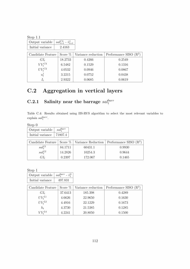
Step 1.1Output variable salC4
t+1 - v1t+1
Initial variance 2.4163
Candidate Feature Score % Variance reduction Performance SISO (R2)
GIt 18.2733 0.4266 0.2549
V V C3t 6.5482 0.1529 0.1316
UV C2t 4.0532 0.0946 0.0867
u1t 3.2215 0.0752 0.0438
It 2.9322 0.0685 0.0619
C.2 Aggregation in vertical layers
C.2.1 Salinity near the barrage salbarrt
Table C.4: Results obtained using IIS-RVS algorithm to select the most relevant variables to
explain salbarrt .
Step 0Output variable salbarrt
Initial variance 71807.4
Candidate Feature Score % Variance Reduction Performance SISO (R2)
salL1t 84.1711 60431.1 0.9930
salL2t 14.2826 10254.3 0.9644
GIt 0.2397 172.067 0.1465
Step 1Output variable salbarrt - v0tInitial variance 497.831
Candidate Feature Score % Variance reduction Performance SISO (R2)
GIt 37.6413 185.398 0.4289
UV L1t 4.6626 22.9650 0.1630
UV L2t 4.4916 22.1229 0.1673
ht 4.3730 21.5385 0.1285
V V L4t 4.2241 20.8050 0.1500
112

C.2.2 Dynamics of salinity in layer 1 salL1t+1
Table C.5: Results obtained using IIS-RVS algorithm to select the most relevant variables to
explain salL1t+1.
Step 0Output variable salL1t+1
Initial variance 120.106
Candidate Feature Score % Variance Reduction Performance SISO (R2)
salL2t 34.1195 40.9388 0.7613
salL1t 14.9457 17.9329 0.7282
salL3t 11.4312 13.7159 0.7428
u2t 8.98024 10.7751 0.1994
salL6t 6.48655 7.78298 0.7017
Step 1Output variable salL1t+1 - v0t+1
Initial variance 28.5366
Candidate Feature Score % Variance reduction Performance SISO (R2)
u2t 50.3218 14.3131 0.6855
GIt 27.187 7.7329 0.5918
u1t 1.9080 0.5427 0.2169
ht 1.5384 0.4376 0.1732
Step 1.1Output variable salL1t+1 - v1t+1
Initial variance 8.0409
Candidate Feature Score % Variance reduction Performance SISO (R2)
GIt 35.72 2.8419 0.300597
UV L2t 6.04684 0.481088 0.0928751
u1t 5.08762 0.404773 0.0615848
UV L3t 3.41868 0.271991 0.0680266
ht 2.85791 0.227377 0.0516562
113
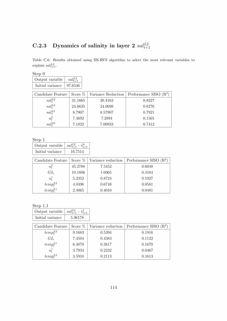
C.2.3 Dynamics of salinity in layer 2 salL2t+1
Table C.6: Results obtained using IIS-RVS algorithm to select the most relevant variables to
explain salL2t+1.
Step 0Output variable salL2t+1
Initial variance 97.6546
Candidate Feature Score % Variance Reduction Performance SISO (R2)
salL2t 31.1665 30.4163 0.8227
salL3t 24.6635 24.0698 0.8276
salL5t 8.7907 8.57907 0.7921
u2t 7.4692 7.2894 0.1565
salL6t 7.1822 7.00933 0.7412
Step 1Output variable salL2t+1 - v0t+1
Initial variance 16.7514
Candidate Feature Score % Variance reduction Performance SISO (R2)
u2t 45.2788 7.5452 0.6048
GIt 10.1806 1.6965 0.4164
u1t 5.2352 0.8724 0.1927
tempL2t 4.0496 0.6748 0.0581
tempL1t 2.4065 0.4010 0.0481
Step 1.1Output variable salL2t+1 - v1t+1
Initial variance 5.96178
Candidate Feature Score % Variance reduction Performance SISO (R2)
tempL2t 9.1683 0.5394 0.1916
GIt 7.4504 0.4383 0.1122
tempL1t 6.4878 0.3817 0.1670
u1t 3.7934 0.2232 0.0467
tempL3t 3.5910 0.2113 0.1613
114

Step 1.2Output variable salL2t+1 - v2t+1
Initial variance 3.50768
Candidate Feature Score % Variance reduction Performance SISO (R2)
GIt 10.8073 0.3712 0.1379
u1t 5.17201 0.1777 0.0640
tempL10t 3.7840 0.1300 0.1070
tempL11t 3.5369 0.1215 0.1029
tempL9t 3.1879 0.1095 0.1037
C.2.4 Dynamics of salinity in layer 3 salL3t+1
Table C.7: Results obtained using IIS-RVS algorithm to select the most relevant variables to
explain salL3t+1.
Step 0Output variable salL3t+1
Initial variance 63.5384
Candidate Feature Score % Variance Reduction Performance SISO (R2)
salL3t 37.1280 23.5887 0.9818
salL4t 23.8781 15.1706 0.9683
salL5t 13.3729 8.49625 0.9134
salL11t 4.7563 3.02186 0.5721
salL10t 4.3524 2.76522 0.5733
Step 1Output variable salL3t+1 - v0t+1
Initial variance 1.14446
Candidate Feature Score % Variance reduction Performance SISO (R2)
u2t 28.9517 0.3302 0.6725
u1t 15.1117 0.1724 0.3010
GIt 7.6087 0.0868 0.4714
ht 4.9324 0.0563 0.2123
It 4.7457 0.0541 0.4544
115

C.2.5 Dynamics of temperature in layer 2 tempL2t+1
Table C.8: Results obtained using IIS-RVS algorithm to select the most relevant variables to
explain tempL2t+1.
Step 0Output variable tempL2t+1
Initial variance 61.2627
Candidate Feature Score % Variance Reduction Performance SISO (R2)
tempL3t 26.2025 16.0475 0.9194
tempL4t 21.6484 13.2584 0.8683
tempL1t 21.0337 12.8819 0.8644
tempL2t 18.5094 11.3359 0.9253
dt 2.7818 1.7037 0.9396
Step 1Output variable tempL2t+1 - v0t+1
Initial variance 3.64568
Candidate Feature Score % Variance reduction Performance SISO (R2)
u2t 20.3046 0.7342 0.3787
GIt 8.5625 0.3096 0.3227
tempL2t 8.3002 0.3001 0.2019
u1t 5.8765 0.2125 0.1181
tempL1t 5.8327 0.2109 0.1563
Step 1.1Output variable tempL2t+1 - v1t+1
Initial variance 1.6907
Candidate Feature Score % Variance reduction Performance SISO (R2)
tempL1t 11.1909 0.1868 0.2674
tempL2t 10.5893 0.1767 0.2883
GIt 5.1110 0.0853 0.0812
tempL3t 2.3815 0.0398 0.1617
u1t 2.0444 0.0341 0.0268
116


Bibliography
M.S. Aldenderfer and R.K. Blachfield. Cluster Analysis. Sage, Beverly Hills, 1984.
M. Amann. Integrated assessment tools. the greenhouse and air pollution interac-
tions and synergies (gains) model. Pollution Atmospherique, pages 73–76, 2009.
M.R. Anderberg. Cluster analysis for applications. Academic Press, New York and
London, 1973.
M. Ankerst, M. Breunig, H.P. Kriegel, and J. Sander. Optics: ordering points
to identify the clustering structure. In Proceedings of the 1999 ACM-SIGMOD
International Conference on Management of Data, Philadelphia, PA, pages 49–60,
1999.
J.P. Antenucci, K.M. Tan, H.S. Eikaas, and Imberger J. The importance of transport
processes and spatial gradients on in-situ estimates of lake metabolism. Hydrobi-
ologia, pages 1–13, 2012.
C.A. Aumann. Constructing model credibility in the context of policy appraisal.
Environmental Modelling & Software, 26(3):258–265, 2011.
V. Babovic. Introducing knowledge into learning based on genetic programming.
Journal of Hydroinformatics, 11(3-4):181–193, 2009.
The World Bank. Dealing with water scarcity in singapore: Institutions, strategies
and enforcement. Technical report, The World Bank, 2006.
R.R. Barton. Simulation metamodels. In Proceedings of the Winter Simulation
Conference, pages 167–174, 1998.
A. Bennett. Inverse modeling of the ocean and atmosphere. Cambridge University
Press, Cambridge, U.K., 2002.
119

J. Beran and G. Mazzola. Visualizing the relationship between time series by hier-
archical smoothing models. Journal of Computational and Graphical Statistics, 8
(2):213–238, 1999.
J.C. Bezdek. Pattern Recognition with Fuzzy Objective Function Algorithms. Plenum
Press, New York and London, 1987.
R.W. Blanning. The construction and implementation of metamodels. Simulation,
24(6):177–184, 1975.
Public Utilities Board. Four taps provide water for all. Technical report, Public
Utilities Board, Singapore, 2005.
G.J. Bowden, G.C. Dandy, and H.R. Maier. Input determination for neural network
models in water resources applications. Journal of Hydrology, 301(1-4):75–92,
2005.
G.E.P. Box and K.B. Wilson. On the experimental attainment of optimum condi-
tions (with discussion). Journal of the Royal Statistical Society Series B, 13(1):
1–45, 1951.
G.A. Carpenter and S. Grossberg. A massively parallel architecture for a self-
organizing neural pattern recognition machine. Computer Vision, Graphics and
Image Process, 37:54–115, 1987.
A. Castelletti and R. Soncini-Sessa. A procedural approach to strengthening inte-
gration and participation in water resource planning. Environmental Modelling &
Software, 21(10):1455–1470, 2006.
A. Castelletti and R. Soncini-Sessa. Bayesian networks and participatory modelling
in water resource management. Environmental Modelling & Software, 22(8):1075–
1088, 2007.
A. Castelletti, S. Galelli, A. Salvetti, and A. Ventimiglia. Extremely Randomized
Trees and Feature Ranking for daily streamflow prediction. In Proceedings of the
9th International Conference on Hydroinformatics. Tianjin, RC., 2010a.
A. Castelletti, S. Galelli, and R. Soncini-Sessa. A tree-based feature ranking ap-
proach to enhance emulation modelling of 3D hydrodynamic-ecological models.
120

In Proceedings of the International Congress on Environmental Modelling and
Software. (eds) IEMSS2010, 2010b.
A. Castelletti, F. Pianosi, R. Soncini-Sessa, and J.P. Antenucci. A multi-
objective response surface approach for improved water quality planning in
lakes and reservoirs. Water Resources Research, 46(W06502), 2010f. doi:
10.1029/2009WR008389.
A. Castelletti, S. Galelli, M. Restelli, and R. Soncini-Sessa. Tree-based feature
selection for dimensionality reduction of large-scale control systems. In Proceedings
of the IEEE Symposium on Adaptive Dynamic Programming and Reinforcement
Learning. Paris, F., 2011.
A. Castelletti, S. Galelli, M. Restelli, and R Soncini-Sessa. Data-driven dynamic em-
ulation modelling for the optimal management of environmental systems. Environ-
mental Modelling & Software, pages –, 2012a. doi: 10.1016/j.envsoft.2011.09.003.
A. Castelletti, S. Galelli, M. Ratto, R Soncini-Sessa, and P. Young. A general frame-
work for dynamic emulation modelling in environmental problems. Environmental
Modelling & Software, pages –, 2012b. doi: 10.1016/j.envsoft.2012.01.002.
P. Cheeseman and J. Stutz. Advances in Knowledge Discovery and Data Mining.,
chapter Bayesian classification (AutoClass): theory and results, pages 153–180.
1996.
L. Chen and V. Ozsu, M.T.and Oria. Robust and fast similarity search for moving
object trajectories. In SIGMOD, 2005.
M.A. Chen, Y. andNascimento, B.C. Ooi, and A.K.H. Tung. Spade: On shape-based
pattern detection in streaming time series. In ICDE, 2007.
V.C.P. Chen, K.L. Tsui, R.R. Barton, and M. Meckesheimer. A review on design,
modeling and applications of computer experiments. Transactions, 38:273–291,
2006.
D.L. Davies and D.W. Bouldin. A cluster separation measure. IEEE Transactions
on Pattern Analysis and Machine Intelligence, 1(2):224–227, 1979.
Deltares. Delft3D-FLOW, Simulation of multi-dimensional hydrodynamic flows and
transport phenomena, including sediments., 2010.
121

H. Ding, G. Trajcevski, P. Scheuermann, X. Wang, and E. Keogh. Querying and
mining of time series data: experimental comparison of representations and dis-
tance measures. In Proceeding of VLDB, Endow., volume 1, pages 1542–1552.
VLDB Endowment, August 2008.
J.C. Dunn. A fuzzy relative of the isodata process and its use in detecting compact
well-separated clusters. Journal of Cybernetics, 3(3):32–57, 1973.
M. Ester, H.P. Kriegel, J. Sander, and X. Xu. A density-based algorithm for discov-
ering clusters in large spatial databases. In Proceedings of the 1996 International
Conference on Knowledge Discovery and Data Mining (KDD’96), Portland, OR,
1996.
B. Everitt. Cluster Analysis. Halsted, New York, 1980.
E. Frentzos, K. Gratsias, and Y. Theodoridis. Index-based most similar trajectory
sear. In ICDE, 2007.
S. Galelli, C. Gandolfi, R. Soncini-Sessa, and D. Agostani. Building a metamodel of
an irrigation district distributed-parameter model. Agricultural Water Manage-
ment, 97(2):187–200, 2010.
P. Geurts and D. Ernst. Extremely randomized trees. Machine Learning, 63(1):
3–42, 2006.
R. Givan, T. Dean, and M. Greig. Equivalence notions and model minimization in
Markov decision processes. Artificial Intelligence, 147(1-2):163–223, 2003.
G.C. Goodwin and R.L. Payne. Dynamic System Identification: Experiment Design
and Data Analysis. Academic Press, New York, N.Y., 1977.
S. Guha, R. Rastogi, and K. Shim. Cure: an efficient clustering algorithm for large
databases. In Proceedings of the 1998 ACMSIGMOD International Conference
on Management of Data, Seattle, WA, pages 73–84, 1998.
I. Guyon and A. Elisseeff. An introduction to variable and feature selection. Journal
of Machine Learning Research, 3:1157–1182, 2003.
I. Guyon, S. Gunn, M. Nikravesh, and L. Zadeh. Feature Extraction, Foundations
and Applications (Series Studies in Fuzziness and Soft Computing). Physica-
Verlag, Springer, Berlin, D., 2006.
122

J. Hartigan. Clustering Algorithms. Wiley, New York, 1975.
J.A. Hartigan. Consistency of single linkage for high-density clusters. Journal of the
American Statistical Association, 76(374):388–394, 1981.
J.A. Hartigan and M.A. Wong. Algorithm as 136: A k-means clustering algorithm.
Journal of the Royal Statistical Society. Series C (Applied Statistics), 28(1):100–
108, 1979.
M.I. Hejazi and X. Cai. Input variable selection for water resources systems us-
ing a modified minimum redundancy maximum relevance (mMRMR) algorithm.
Advances in Water Resources, 32(4):582–593, 2009.
A.K. Jain and R.C. Dubes. Algorithms for Clustering Data. Prentice Hall, Engle-
wood Cliffs, New Jersey, 1988.
A.K. Jain, M.N. Murty, and P.J. Flynn. Data clustering: a review. ACM Computing
Surveys, 31(3):264–323, 1999a.
Anil K. Jain, M. Narasimha Murty, and Patrick J. Flynn. Data clustering: a review.
ACM Computing Surveys - CSUR, 31(3):264–323, 1999b.
A. Janssen and H. Ogink. Singapore marina reservoir study.hydrological and hy-
draulic model report. Technical report, Delft, The Netherlands, Deltares, 2007.
N. Jardine and R. Sibson. Mathematical Taxonomy. Wiley, London, 1971.
I.T. Jollife. Principal Component Analysis. Springer, New York, NY., 1986.
K. Jong, J. Mary, A. Cornuejols, E. Marchiori, and M. Sebag. Ensemble feature
ranking. Springer, Verlag, 2004.
E. Kalnay. Atmospheric Modeling, Data Assimilation, and Predictability. Cambridge
University Press, Cambridge, U.K., 2002.
G. Karypis, E.H. Han, and V. Kumar. Chameleon: hierarchical clustering using
dynamic modeling. Computer, pages 68–75, 1999.
L. Kaufman and P.J. Rousseeuw. Finding Groups in Data: An Introduction to
Cluster Analysis. Wiley, New York, 1990.
123

E.J. Keogh and C.A. Ratanamahatana. Exact indexing of dynamic time warping.
Data Mining and Knowledge Discovery, 3(3):263–286, 2005.
J.P.C. Kleijnen. Response surface methodology for constrained simulation optimiza-
tion: An overview. Simulation Modelling Practice and Theory, 16(1):50–64, 2008.
T. Kohonen. The self-organizing map. In Proceedings of the IEEE, 1990.
K. Kosmelj and V. Batagelj. Cross-sectional approach for clustering time varying
data. Journal of Classification, pages 99–109, 1990.
R. Krishnapuram, A. Joshi, O. Nasraoui, and L. Yi. Low complexity fuzzy relational
clustering algorithms for web mining. IEEE Trans. Fuzzy Systems, 9(4):595–607,
2001.
J.A. Lee and M. Verleysen. Nonlinear Dimensionality Reduction. Springer, New
York, NY., 2007.
T.W. Liao. Clustering of time series data - a survey. Pattern Recognition, 38(11):
1857–1874, 2005.
S.C. Liew, S.Y. Liong, and M.T. Vu. A study of urban stormwater modeling ap-
proach in singapore catchment. Advances in Geosciences, Hydrological Science
(HS), 23:89–101, 2001.
M. Lorr. Cluster analysis for social scientists. Jossey-Bass (San Francisco), 1983.
J. MacQueen. Some methods for classification and analysis of multivariate observa-
tions. In L.M. LeCam and J. Neyman, editors, Proceedings of the Fifth Berkeley
Symposium on Mathematical Statistics and Probability, volume 1, pages 281–297,
1967.
P. Magni, F. Ferrazzi, L. Sacchi, and R. Bellazzi. Timeclust: a clustering tool
for gene expression time series. Bioinformatics Application Note, 24(3):430–432,
2008.
R.J. May, H.R. Maier, G.C. Dandy, and T. Fernando. Non-linear variable selection
for artificial neural networks using partial mutual information. Environmental
Modelling and Software, 23(10-11):1312–1326, 2008a.
124
R.J. May, G.C. Dandy, H.R. Maier, and J.B. Nixon. Application of partial mutual
information variable selection to ANN forecasting of water quality in water dis-
tribution systems. Environmental Modelling and Software, 23(10-11):1289–1299,
2008b.
M. Nayak and S. Dash. Gpac-apso clustering using modified s-transform for data
mining. International Journal of Engineering Science and Advanced Technology,
2(1):38–48, 2012.
H. Peng, F. Long, and C. Ding. Feature selection based on mutual information: cri-
teria of max-dependency, max-relevance, and minimum redundancy. IEEE Trans-
actions on Pattern Analysis and Machine Intelligence, 27(8):1226–1238, 2005.
N.V. Queipo, R.T. Haftka, W. Shyy, T. Goel, R. Vaidyanathan, and P.K. Tucker.
Surrogate-based analysis and optimization. Progress in Aerospace Sciences, 41
(1):1–28, 2005.
E. Rendon, I. Abundez, A. Arizmendi, and E.M. Quiroz. Internal versus external
cluster validation indexes. International Journal of Computers and Communica-
tion, 5(1):27–34, 2011.
H.C. Romesburg. Cluster Analysis for Researchers. Lifetime Learning, California,
1984.
J. Sacks, W.J. Welch, T.J. Mitchell, and H.P. Wynn. Design and analysis of com-
puter experiments. Statistical Science, 4(4):409–435, 1989.
N. Sadegh. Minimal realization of nonlinear systems described by input-output
difference equations. IEEE Transactions on Automatic Control, 46(5):698–710,
2001.
A. Saltelli, K. Chan, and M. Scott. Sensitivity Analysis. Wiley, New York, NY.,
2000.
A. Saltelli, S. Tarantola, F. Campolongo, and M. Ratto. Sensitivity analysis in
practice. A guide to assessing scientific models. John Wiley & Sons, Ltd, Hoboken,
NJ., 2004.
A. Saltelli, M. Ratto, T. Andres, F. Campolongo, J. Cariboni, D. Gatelli, M. Saisana,
and S. Tarantola. Global Sensitivity Analysis. The Primer. John Wiley & Sons,
Ltd, Hoboken, NJ., 2008.
125
L.M. See, A. Jain, C.W. Dawson, and R.J. Abrahart. Visualisation of hidden neuron
behaviour in a neural network rainfall-runoff model. In: Practical Hydroinformat-
ics. Water Science and Technology Library, 2008.
S. Selvalingam, S.Y. Liong, and P.C. Manoharan. Use of RORB and SWMM models
to an urban catchment in Singapore. Advances in Water Resources, 10(2):78–86,
1987.
C. Shaw and G.P. King. Using cluster analysis to classify time series. Physica D:
Nonlinear phenomena, 58:288–298, 1992.
T.W. Simpson, J.D. Peplinski, P.N. Koch, and J.K. Allen. Metamodels for com-
puter based engineering design: survey and recommendations. Engineering with
Computers, 17(2):129–150, 2001.
J. Smits and Beek J.V. Marina reservoir study: Water quality mitigation scenario
analysis. Technical report, Delft, The Netherlands, Deltares, 2007a.
J. Smits and Beek J.V. Marina reservoir study. water quality modelling. Technical
report, Delft, The Netherlands, Deltares, 2007b.
R.R. Sokal and C.D. Michener. A Statistical Method for Evaluating Systematic
Relationships., volume 28. University of Kansas Scientific Bulletin, 1958.
T. Sorensen. A Method of Establishing Groups of Equal Amplitude in Plant Sociology
Based on Similarity of Species Content and Its Application to Analyses of the
Vegetation on Danish Commons., volume 5. Biologiske Skrifter, 1948.
D. Twigt and D. Burger. Water quality operational management system (wq
oms), functional and technical design. Technical report, Delft, The Netherlands,
Deltares, 2010.
J.J. Van Wijk and E.R. Van Selow. Cluster and calendar based visualization of time
series data. In Proceedings of IEEE Symposium on Information Visualization,
San Francisco, CA, October 25-26 1999.
M. Vlachos, D. Gunopulos, and G. Kollios. Discovering similar multidimensional
trajectories. In ICDE, 2002.
A. Voinov and F. Bousquet. Modelling with stakeholders. Environmental Modelling
& Software, 25(11):1268–1281, 2010.
126

W. Wang, J. Yang, and R. Muntz. Sting: a statistical information grid approach to
spatial data mining. In Proceedings of the 1997 International Conference on Very
Large Data Base (VLDB’97), Athens, Greek, pages 186–195, 1997.
L. Wehenkel. Automatic Learning Techniques in Power Systems. Kluwer Academic,
Boston, MA., 1998.
H.S. Wheater, A.J. Jakeman, and K.J. Beven. Modelling Change in Environmental
Systems. IWA Publishing, Wiley, Chichester, U.K., 1993.
K. Willcox and J. Peraire. Balanced model reduction via the proper orthogonal
decomposition. AIAA Journal, 40(11):2323–2330, 2002.
Y. Xiong and D.Y. Yeung. Mixtures of arma models for model-based time series
clustering. In Proceedings of the IEEE International Conference on Data Mining,
Maebaghi City, Japan, December 9-12 2002.
B.-K. Yi and C. Faloutsos. Fast time sequence indexing for arbitrary lp norms. In
VLDB, 2000.
P. C. Young and M. Ratto. A unified approach to environmental systems modeling.
Stochastic Environmental Research and Risk Assessment, 23:1037–1057, 2009.
P. C. Young and M. Ratto. Statistical emulation of large linear dynamic models.
Technometrics, 53(1):29–43, 2011.
P.C. Young. Data-based mechanistic modeling of environmental, ecological, eco-
nomic and engineering systems. Environmental Modelling & Software, 13(2):105–
122, 1998.
T. Zhang, R. Ramakrishnan, and M. Livny. Birch: an efficient data clustering
method for very large databases. In Proceedings of the 1996 ACM-SIGMOD
International Conference on Management of Data, Montreal, Canada, pages 103–
114, 1996.
W. Zhang and B. Michaelis. Shape control with karhunen-love decomposition: The-
ory and experimental results. Journal of Intelligent Material Systems and Struc-
tures, 14(7):415–422, 2003.
F. Zijl and D. Twigt. Singapore marina reservoir study. hydrodynamic modelling.
Research Report Z.4265.10/20/30, Deltares, 2007.
127


