improved corrections process for constrained trajectory

Improved Corrections Process for Constrained Trajectory Designin the n-Body Problem

Belinda G. Marchand∗ and Kathleen C. Howell†

Purdue University, West Lafayette, Indiana 47907-1282

and

Roby S. Wilson‡

Jet Propulsion Laboratory, California Institute of Technology, Pasadena, California 91109

DOI: 10.2514/1.27205

The general objective is the development of efficient techniques for preliminary design of trajectory arcs in

nonlinear autonomous dynamic systems in which the desired solution is subject to algebraic interior and/or exterior

constraints. For application to then-body problem, trajectoriesmust satisfy specific requirements, e.g., periodicity in

terms of the states, interior or boundary constraints, and specified coverage. Thus, a strategy is formulated in a

sequence of increasingly complex steps: 1) a trajectory isfirstmodeled as a series of arcs (analytical or numerical) and

general trajectory characteristics and timing requirements are established; 2) the specific constraints and associated

partials are formulated; 3) a corrections process ensures position and velocity continuity while satisfying the

constraints; and finally, 4) the solution is transitioned to a full model employing ephemerides. Though the examples

pertain to spacecraft mission design, the methodology is generally applicable to autonomous systems subject to

algebraic constraints. For spacecraft mission design applications, an immediate advantage of this approach,

particularly for the identification of periodic orbits, is that the startup solution need not exhibit any symmetry to

achieve the objectives.

Nomenclature

Ak;k�1, Bk;k�1,Ck;k�1, Dk;k�1

= 3 � 3 submatrices of ��tk; tk�1�

A�t� = Jacobian matrixa�t� � � �x; �y; �z�T = column vector that denotes the

spacecraft acceleration, km=s2

f�X� = a nonlinear vector function that dependsexplicitly on the spacecraft state

N = number of patch states along a startupsolution

R�t� � �x; y; z�T = column vector that denotes spacecraftposition, km

t = time, sV�t� � � _x; _y; _z�T = column vector that denotes spacecraft

velocity, km=sX�t� � �R�t�;V�t��T = column vector that denotes the

spacecraft statex, y, z = spacecraft position elements associated

with current working reference frame,km

_x, _y, _z = spacecraft velocity elements associatedwith current working reference frame,km=s

�k = vector of constraints at the kth patchstate

�kj = the jth element of �k�Vk = velocity discontinuity at the kth patch

state, km=s� = prefix denotes a variation measured

relative to a reference arc��tk; tk�1� = 6 � 6 state transition matrix from an

initial time tk�1 to a terminal time tk

Subscripts

k = subscript indicates the quantity isassociated with the kth patch state

Superscripts

T = superscript denotes transpose operation� = superscript indicates the quantity is

evaluated along the reference solution

Introduction

F ROM a dynamic perspective, the libration points have been thefocus of many investigations since the initial work of Poincaré

[1]. In the last 20 years, periodic orbits in the three-body regime havesuccessfully served as the basis for trajectory design in variousmissions [2–8], from the International Sun-Earth Explorer 3 (ISEE-3) [2,3] to the more recent Genesis mission [8]. As the spacecraftapplications of multibody orbital analysis continue to expand, thegoals and requirements are also becoming evermore challenging.Thus, strategies to isolate preliminary trajectory arcs that satisfy a setof constraints in this regime must be available.

Most optimization schemes, or other analysis tools in the fullmodel, require a good initial guess or startup solution. Thus, the goalof this study is the development of a strategy to more efficientlyproduce preliminary designs for trajectories, in multibody regimes,when constraints are incorporated. Though the examples presentedare related to spacecraft mission design in the n-body problem, thegenerality of the method is preserved to accommodate otherapplications. Ultimately, this approach represents a feasiblenumerical scheme for the determination of trajectory arcs innonlinear autonomous dynamic systems where the desired solutionis subject to algebraic interior and/or exterior constraints.

Received 10 August 2006; accepted for publication 17 January 2007.Copyright©2007 byBelindaG.Marchand,KathleenC.Howell, andRobyS.Wilson. Published by the American Institute of Aeronautics andAstronautics, Inc., with permission. Copies of this paper may be made forpersonal or internal use, on condition that the copier pay the $10.00 per-copyfee to the Copyright Clearance Center, Inc., 222 Rosewood Drive, Danvers,MA 01923; include the code 0022-4650/07 $10.00 in correspondence withthe CCC.

∗Visiting Assistant Professor, School of Aeronautics and Astronautics,PurdueUniversity; currentlyAssistant Professor, Aerospace Engineering andEngineering Mechanics Department, University of Texas at Austin.

†Hsu Lo Professor of Aeronautical and Astronautical Engineering, Schoolof Aeronautics and Astronautics, Purdue University.

‡Senior Engineer, Guidance Navigation and Control Section, JetPropulsion Laboratory.

JOURNAL OF SPACECRAFT AND ROCKETS

Vol. 44, No. 4, July–August 2007

884

http://dx.doi.org/10.2514/1.27205

The approach proposed here involves a sequence of increasinglycomplex steps [9,10]. Initially, the trajectory ismodeled as a series ofarcs. The arcs may be determined from a three-body model, amultibody numerical solution, or a conic. An arc can also incorporatesome additional force, if appropriate, such as solar radiation pressure.This initial analysis is useful in establishing the general trajectorycharacteristics such as size, orientation, excursions in the in-planeand out-of-plane directions, proximity to specified regions of space(perhaps the libration points), and timing requirements. In the nextstep in the process, the specific constraints aremodeled, aswell as theassociated partials, if not already available. Then, a differentialcorrections process is employed to ensure position and velocitycontinuity along the path while satisfying the constraints. Theprocess can also be used to determine preliminary requirements formaneuvers that may be necessary to satisfy the constraints. In thefinal step, the trajectory solution is transitioned to a full model thatincorporates any desired gravitational bodies,with ephemerides usedfor the planetary locations. It may include other forces, such as solarradiation pressure, as modeled previously. The focus of this effort,then, is the further development of the mathematical relationshipsand partials that are necessary to successfully merge the arcs in thethree- or n-body environment such that the constraints are satisfied.

Background

In generating a preliminary solution, the capacity to develop atrajectory arc in the three- or four-body problem, one that satisfies aset of constraints, is considered critical for an expanded design tool.For instance, a halo orbit [11] is periodic and symmetric across afundamental plane in the rotating frame of the restricted problem.Symmetry and periodicity are both, in this case, constrained.However, an orbit can be periodic without being symmetric [12], asis often the case in relative spacecraft motions [13] (i.e., formationflight) near the libration points.

In the restricted three-body problem, where the equations ofmotion are traditionally formulated in a synodic coordinate system, atypical approach to determine a periodic path is to exploit thesymmetry of themathematical model. First, a startup arc, such as thatobtained from the Richardson approximation [14,15], is necessary.Once the startup solution is available, the symmetry properties of themodel and the solution of interest, are employed in the design of thedifferential corrector [11]. However, a differential correctorspecifically developed around some geometrical features willnaturally only be applicable to trajectories that share those features.Atraditional halo corrector, for example, is only useful when searchingfor trajectories that are simply symmetric about the x–z plane.

As detailed in this investigation, it is possible to specify periodicityas a constraint, without prior knowledge of the symmetry of thesolution. Using periodicity as a constraint is particularly useful inexploring periodic orbits near the triangular points, or establishingperiodic formations near the libration points. In general, trajectoryarcs of any kind can be subject to a wide variety of point constraintsduring the mission design process. The development is generalizedand applicable to any type of point constraint. It is assumed, ofcourse, that the initial guess is still in the vicinity of the desiredsolution.

Dynamic Model

The elements of the spacecraft state vectorX�t� � �x�t�; y�t�; z�t�;_x�t�; _y�t�; _z�t��T represent components of the spacecraft position andvelocity, associated with a generic reference frame. Based on thisdefinition, the nonlinear differential equations that govern theevolution of X�t�, in any gravitational regime, may be generallyrepresented as

_X�t� � f �X�t�� (1)

LetX��t� and _X��t� identify a reference state, and the associated time

derivative. Then, according to Eq. (1), _X��t� � f �X��t��. Thegeneral nonlinear state of the spacecraft can always be representedrelative to this reference state as follows:

X �t� �X��t� �X�t� (2)

From the definition in Eq. (2), the variational equation associatedwith Eq. (1) is of the form

� _X�t� � A�t��X�t� (3)

where

A�t� � @f@X

��X��t�

(4)

represents the Jacobian matrix evaluated along the referencesolution. The solution to this variational equation is well known anddepends on the state transition matrix (STM) ��t; t0�:

�X�t� ��t; t0��X�t0� (5)

The STM is determined by numerical integration of the matrixdifferential equation

_��t; t0� � A�t��t; t0� (6)

subject to the initial condition ��t0; t0� � I, where I denotes aproperly dimensioned identity matrix. The variation in Eq. (5) isgenerally said to be contemporaneous. That is, the variation �X�t� isthe difference between the actual nonlinear state X�t� and theneighboring nominal state X��t�, evaluated precisely at time t.However, the derivation of a differential corrections process benefitsfrom the introduction of a noncontemporaneous variation,

�X0 � � �X�t0� � �X�t� _X�t��t (7)

where �t� t0 � t and _X is evaluated along the current (i.e., thereference) solution. The relation between the contemporaneous andnoncontemporaneous variation is illustrated graphically in Fig. 1.

Substitution of Eq. (7) into Eq. (5) yields the following expression:

��X01 � _X�t1��t1� ��t1; t0��X00 � _X�t0��t0� (8)

If the initial time for the numerical propagation is held fixed, relativeto the nominal initial time, then �t0 � 0 and Eq. (8) can be furtherreduced, i.e.,

�X01 ��t1; t0��X00 _X1�t1 (9)

Equation (9) is the basis of a standard two-level differential corrector.

Startup Arcs and Patch States

A differential corrections process requires a startup solution. Sucha trajectory arc may be the result of a numerical integration process[16], perhaps one such that the path does not necessarily satisfy thespecified constraints. An initial guess can also be constructed from aseries expansion [14,15] that approximates the solution.

Fig. 1 Contemporaneous vs noncontemporaneous variations.

MARCHAND, HOWELL, AND WILSON 885

Other alternatives, even conics, can also serve as a startup arc inthe ephemeris model. Once available, the startup solution isdecomposed into segments and nodes, or patch points. The processof selecting patch points is somewhat open-ended. It is important,however, that the patch points that are selected adequately capturethe overall character and geometry of the solution to ensureconvergence. At the same time, too many patch points canunnecessarily constrain the search process and limit the solutionspace that the corrector is able to identify. For instance, a Lissajoustrajectory in the n-body problem is geometrically well behaved.However, due to the dynamically sensitive nature of the region nearthe libration points, it is best to select at least four patch points perrevolution. Although two patch points may be sufficient to convergeon a Lissajous trajectory, four will ensure that the overall dimensionsof the startup arc are preserved if at all possible. These four patchpointsmay be placed, for instance, at each of themaximumexcursionpoints along the y and z directions in the synodic rotating frame.

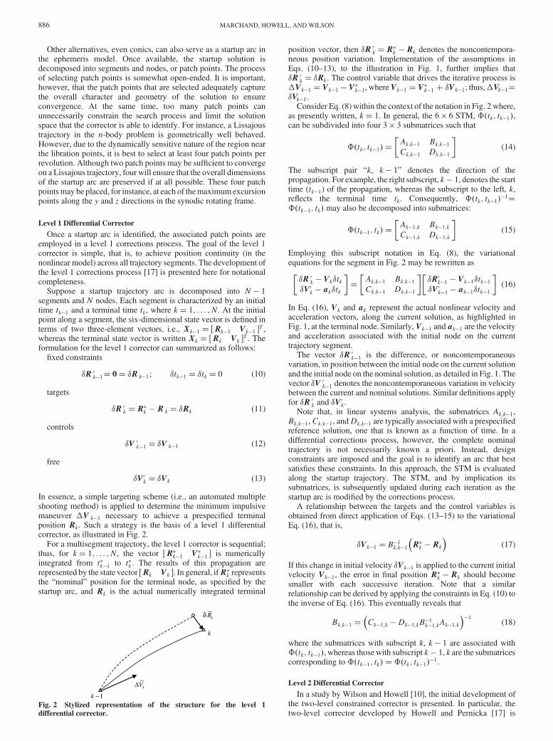
Level 1 Differential Corrector

Once a startup arc is identified, the associated patch points areemployed in a level 1 corrections process. The goal of the level 1corrector is simple, that is, to achieve position continuity (in thenonlinear model) across all trajectory segments. The development ofthe level 1 corrections process [17] is presented here for notationalcompleteness.

Suppose a startup trajectory arc is decomposed into N � 1segments and N nodes. Each segment is characterized by an initialtime tk�1 and a terminal time tk, where k� 1; . . . ; N. At the initialpoint along a segment, the six-dimensional state vector is defined interms of two three-element vectors, i.e., Xk�1 � �Rk�1 Vk�1 �T ,whereas the terminal state vector is written Xk � �Rk Vk �T . Theformulation for the level 1 corrector can summarized as follows:

fixed constraints

�R 0k�1� 0� �R k�1; �tk�1 � �tk � 0 (10)

targets

�R 0k �R�k � R k � �Rk (11)

controls

�V 0k�1 � �V k�1 (12)

free

�V0k � �Vk (13)

In essence, a simple targeting scheme (i.e., an automated multipleshooting method) is applied to determine the minimum impulsivemaneuver �V k�1 necessary to achieve a prespecified terminalposition Rk. Such a strategy is the basis of a level 1 differentialcorrector, as illustrated in Fig. 2.

For a multisegment trajectory, the level 1 corrector is sequential;thus, for k� 1; . . . ; N, the vector �R�k�1 V�k�1 � is numericallyintegrated from t�k�1 to t�k . The results of this propagation arerepresented by the state vector �Rk Vk �. In general, ifR�k representsthe “nominal” position for the terminal node, as specified by thestartup arc, and Rk is the actual numerically integrated terminal

position vector, then �R 0k �R�k � Rk denotes the noncontempora-neous position variation. Implementation of the assumptions inEqs. (10–13), to the illustration in Fig. 1, further implies that�R 0k � �Rk. The control variable that drives the iterative process is�Vk�1 � Vk�1 � V�k�1, whereVk�1 � V�k�1 �Vk�1; thus,�Vk�1��Vk�1.

Consider Eq. (8) within the context of the notation in Fig. 2 where,as presently written, k� 1. In general, the 6 � 6 STM, ��tk; tk�1�,can be subdivided into four 3 � 3 submatrices such that

��tk; tk�1� �Ak;k�1 Bk;k�1Ck;k�1 Dk;k�1

� �(14)

The subscript pair “k, k � 1” denotes the direction of thepropagation. For example, the right subscript, k � 1, denotes the starttime (tk�1) of the propagation, whereas the subscript to the left, k,reflects the terminal time tk. Consequently, ��tk; tk�1��1��tk�1; tk� may also be decomposed into submatrices:

��tk�1; tk� �Ak�1;k Bk�1;kCk�1;k Dk�1;k

� �(15)

Employing this subscript notation in Eq. (8), the variationalequations for the segment in Fig. 2 may be rewritten as

�R 0k � Vk�tk�V0k � ak�tk

� �� Ak;k�1 Bk;k�1

Ck;k�1 Dk;k�1

� ��R0k�1 � Vk�1�tk�1�V0k�1 � ak�1�tk�1

� �(16)

In Eq. (16), Vk and ak represent the actual nonlinear velocity andacceleration vectors, along the current solution, as highlighted inFig. 1, at the terminal node. Similarly,Vk�1 and ak�1 are the velocityand acceleration associated with the initial node on the currenttrajectory segment.

The vector �R 0k�1 is the difference, or noncontemporaneousvariation, in position between the initial node on the current solutionand the initial node on the nominal solution, as detailed in Fig. 1. Thevector �V 0k�1 denotes the noncontemporaneous variation in velocitybetween the current and nominal solutions. Similar definitions applyfor �R 0k and �V

0k.

Note that, in linear systems analysis, the submatrices Ak;k�1,Bk;k�1,Ck;k�1, andDk;k�1 are typically associated with a prespecifiedreference solution, one that is known as a function of time. In adifferential corrections process, however, the complete nominaltrajectory is not necessarily known a priori. Instead, designconstraints are imposed and the goal is to identify an arc that bestsatisfies these constraints. In this approach, the STM is evaluatedalong the startup trajectory. The STM, and by implication itssubmatrices, is subsequently updated during each iteration as thestartup arc is modified by the corrections process.

A relationship between the targets and the control variables isobtained from direct application of Eqs. (13–15) to the variationalEq. (16), that is,

�Vk�1 � B�1k;k�1�R�k � Rk

�(17)

If this change in initial velocity �Vk�1 is applied to the current initialvelocity Vk�1, the error in final position R�k � Rk should becomesmaller with each successive iteration. Note that a similarrelationship can be derived by applying the constraints in Eq. (10) tothe inverse of Eq. (16). This eventually reveals that

Bk;k�1 ��Ck�1;k �Dk�1;kB

�1k�1;kAk�1;k

��1(18)

where the submatrices with subscript k, k � 1 are associated with��tk; tk�1�, whereas those with subscript k � 1, k are the submatricescorresponding to ��tk�1; tk� ��tk; tk�1��1.

Level 2 Differential Corrector

In a study by Wilson and Howell [10], the initial development ofthe two-level constrained corrector is presented. In particular, thetwo-level corrector developed by Howell and Pernicka [17] is

kRδ

kV∆

1k −

k

Fig. 2 Stylized representation of the structure for the level 1

differential corrector.

886 MARCHAND, HOWELL, AND WILSON

augmented with terminal boundary constraints on radial distance,time, inclination, apse condition, and state.

The process is applied to the initial design of the Genesistrajectory. In the present investigation, a generalization of thismethodology is developed and implemented as an end-to-endmission design tool.

The level 2 differential corrector is a procedure based on three ormore patch points. The goal of the level 2 corrector is tosimultaneously determine a set of adjustments, or modifications, inthe state elements for all of the nodes (or patch points) to meet somegiven set of constraints. Of theN nodes available, the first and last aretermed the initial and final states. All the remaining nodes are termedinterior patch points.Hence, if there areN patch points, thenN � 2 ofthese nodes are interior patch points.

An example problem with three patch points is represented inFig. 3, where the subscript k � 1 denotes the initial state along onesegment, k 1 identifies the final state on the next segment, and k isassociated with the interior state that connects the two consecutivesegments. The state vector at the initiation of a numericalpropagation process is labeled with a superscript, whereas that atthe end of a propagation is labeledwith the� superscript. The goal ofthe level 1 corrections process is to achieve position continuity acrosssegments Rk �R�k . Once position continuity is achieved, the nextlevel of the corrections process enforces any given number ofconstraints on any of the N patch points available. For instance,Howell and Pernicka [17] employ a two-level corrector to enforcevelocity continuity at each of the interior points. In this case, threescalar constraints are imposed on each interior point, Vk � V�k fork� 2; . . . ; N � 1.

Velocity continuity across segments is formulated as a constraint[10,17], applied at the kth node, such that Vk � V�k ��V�k � 0,where�V�k represents the desired value of the impulsivemaneuver atthe kth node. Then, the goal of a level 2 corrections process is tominimize the constraint error.

The control variables available to enforce the constraints at thenodes are the positions and times associated with the nodesthemselves. Thus, the patch points in the level 2 corrector are allowedto “float” in a sense.

The next step in a generalized level 2 corrector is to establish arelationship between the control variables and the constraintequations. To that end, consider the following set of variationalequations associated with each of the segments in Fig. 3, i.e.,

��R 0k�� V�k �t�k��V0k�� a�k �t�k

� �

� Ak;k�1 Bk;k�1Ck;k�1 Dk;k�1

� ��R 0k�1� � Vk�1�tk�1��V 0k�1� � ak�1�tk�1

� �(19)

��R0k� � Vk �tk��V0k� � ak �tk

� �

� Ak;k1 Bk;k1Ck;k1 Dk;k1

� ��R0k1�� V�k1�t�k1��V0k1�� a�k1�t�k1

� �(20)

Note that, in Eq. (20), the flow of the second segment is reversed toevolve from tk1 to tk. In the present development, each trajectorysegment is treated independently with respect to the rest of thesegments along the solution. For example, the variations in the initialstate at tk�1 do not directly affect changes on the second segment,from tk to t�k1. This segment independence results directly from thesequential nature of the level 1 corrector. Using the sameterminology employed previously, the formulation for this particularlevel 2 differential corrector is as follows:

fixed constraints

�Rk � �R�k � �0; tk � t�k � 0 (21)

targets ��Vk � �V�k

�� V�k � � �Vk � � �V�k �� V�k (22)

controls

� �Rk�1; �tk�1; � �Rk; �tk; � �Rk1; �tk1 (23)

free

� �Vk�1; � �V�k1 (24)

Note that, if a deterministic maneuver is allowed at the kth node, then�V�k ≠ 0. Based on Eq. (22), there are �N � 2� � 3 targets, three foreach interior patch point. The control variables, as previously stated,are the position and times of allN patch points. Thus, in general, thereare N � 4 control parameters. Beyond the initial investigation byHowell and Pernicka [17], it is also possible to specify arbitraryconstraints at any of the N patch points [10]. These constraintsbecome additional targets in a level 2 corrections process. In thefollowing section, additional constraints are presented to supplementthose originally presented byWilson andHowell [10] and expand thegenerality of the method. Note that, unless too many constraints arespecified, this system will naturally be underdetermined.

To solve the subproblem in Fig. 3, it is necessary to relate the targetto the control variables, �R k�1, �tk�1, �Rk, �tk, �Rk1, and �tk1. Inthe case of the velocity continuity constraint, the followingapproximations are necessary:

�V�k ��@V�k@R k�1

��R k�1

�@V�k@tk�1

��tk�1

�@V�k@Rk

��Rk

�@V�k@tk

��tk (25)

�Vk ��@Vk@Rk

��Rk

�@Vk@tk

��tk

�@Vk@Rk1

��Rk1

�@Vk@tk1

��tk1 (26)

In the level 2 formulation, the partial derivatives are evaluated alongthe current trajectory. As a result, the variations are defined as�V�k � �V�k �� V�k and �Vk � �Vk �� Vk , and the velocitycontinuity constraint is

�Vk � �V�k ��Vk

�� V�k �� Vk � V�k ��V�k ��Vk

(27)

This function can be obtained by subtracting Eq. (26) from Eq. (25):

��Vk ��V�k ��Vk �� @V�k@R k�1

��Rk�1

�� @V

�k

@tk�1

��tk�1

�@Vk@Rk� @V

�k

@Rk

��Rk

�@Vk@tk� @V

�k

@tk

��tk

�@Vk@Rk1

��Rk1

�@Vk@tk1

��tk1 (28)

Fig. 3 Stylized representation of level 2 differential corrector.


Equation (28) is basically a Taylor series expansion of�Vk; hence,the definitions in Table 1 are immediately apparent.

The determination of each of the partial derivatives in Table 1 isaccomplished through a finite difference approach. For example, toisolate the variation ofV�k with respect toR k�1, all other independentcontrol variables are set to zero in the variational equations for therelevant segment

�Rk � �Rk1 � 0 (29)

�tk�1 � �tk � �tk1 � 0 (30)

As a result, the partial derivative can be approximated as@V�k =@Rk�1 �V�k =�Rk�1. The variations necessary to constructthese partials may be obtained through algebraic manipulation of thevariational Eqs. (19) or (20). The results of this finite differenceapproximation are presented in Table 2.

For the level 2 velocity continuity constraint, substitution of thepreceding partials into the expressions in Table 1 leads to the resultsin Table 3. The traditional statement [17] of the level 2 corrector is

��Vk ��V�k ��Vk

� @�Vk@Rk�1

@�Vk@tk�1

@�Vk@Rk

@�Vk@tk

@�Vk@Rk1

@�Vk@tk1

h i|��{z��}

M

�R k�1�tk�1�Rk�tk�Rk1�tk1

26666664

37777775

|��{z��}b

(31)

In Eq. (31), the matrixM, containing all of the partial derivatives inTable 3, is termed the state relationship matrix (SRM) and b denotesthe vector of variations in position and time. The linear system inEq. (31) can subsequently be summarized as ��Vk �Mb.

In a well-posed problem, the system is underdetermined; that is,there are more control variables than target quantities. Hence, aninfinite number of solutions exist. In a traditional corrections process,the minimum Euclidean norm solution is selected. The minimum-norm solution is well known and computed as

b �MT�MMT��1��Vk (32)

The results from Eq. (32) suggest possible changes in the positionsand times of each patch state that may minimize the constraintequations. These changes are applied in the nonlinear system and thelevel 1 iteration is repeated to achieve position continuity. Of course,the changes suggested by Eq. (32) only lead to a minimum-normsolution in the linear system. In reality, it is unlikely that themodifiednonlinear path will exactly satisfy the constraints after positioncontinuity is reestablished in the nonlinear system.

At best, the updated nonlinear path will more closely follow thegiven constraints. Ultimately, if a solution exists in the nonlinearsystem, the interior values of�Vk should decrease, or approach thenominal value, with every successive iteration.

Level 2 with Constraints

It is frequently necessary to specify additional constraints along aparticular trajectory. The level 2 differential corrector described inthe preceding section can be modified to allow general constraints atany of the patch points that describe the solution. Incorporatingconstraints at any patch point is possible as long as the constraint is ofthe form

�kj � �kj�Rk;V

k ;V

�k ; tk

�(33)

or

�kj � �kj�Rk;Vk; tk� (34)

Thus, the scalar constraint �kj must be expressed as a function of theposition, velocity, and time that correspond to the patch point. Thefirst subscript index, k, on the constraint denotes the patch point withwhich the constraint is associated. The second index j denotes theconstraint number at that patch point. This allows for multipleconstraints at multiple patch points. Let ��kj represent the desired

value of this algebraic constraint. Recall that the control variables in alevel 2 corrector are �R k�1, �tk�1, �Rk, �tk, �Rk1, and �tk1. Toincorporate these constraints into the corrections process, it isnecessary to establish a relationship between the targets,��kj � ��kj � �kj, and the control variables. By definition, �kj candepend explicitly on Rk and tk. However, there is no explicitdependence on the remaining control variables. Instead, theconstraint may also depend on either Vk or V�k , or both. Such afunctional form introduces an implicit dependence on the othercontrol variables because the velocity discontinuities at the kth patchpoint are related to the position and times of the nodes neighboringthe patch point of interest; in particular,

V k � Vk �Rk; tk;Rk1; tk1� (35)

V �k � V�k �Rk�1; tk�1;Rk; tk� (36)

Thus, the constraint equation can also be approximated, to the firstorder, through the following Taylor series expansion:

Table 1 Level 2 partial derivatives of velocity

discontinuity across patch states

Partials with respect to position Partials with respect to time

@�Vk@R k�1

�� @V�

k

@R k�1

�@�Vk@tk�1�� @V�

k

@tk�1

�@�Vk@Rk��@V

k

@Rk� @V�

k

@Rk

�@�Vk@tk��@V

k

@tk� @V�

k

@tk

�@�Vk@Rk1��@V

k

@Rk1

�@�Vk@tk1��@V

k

@tk1

�

Table 2 Partial derivatives of velocity relative to patch state

control variables


@V�k

@R k�1� B�1k�1;k

@V�k

@tk�1��B�1k�1;kVk�1

@V�k

@Rk��B�1k�1;kAk�1;k

@V�k

@tk��a�k �Dk;k�1B

�1k;k�1V

�k

�@V

k

@Rk��B�1k1;kAk1;k

@Vk

@tk��ak � Dk;k1B

�1k;k1V

k

�@V

k

@Rk1� B�1k1;k

@Vk

@tk1��B�1k1;kV�k1

Table 3 Summary of partial derivatives for level 2: velocity constraints at interior patch

points


@�Vk@R k�1

��B�1k�1;k @�Vk@tk�1� B�1k�1;kVk�1

@�Vk@Rk� B�1k�1;kAk�1;k � B�1k1;kAk1;k @�Vk

@tk� ak � a�k Dk;k�1B

�1k;k�1V

�k � Dk;k1B

�1k;k1V

k or

@�Vk@tk� ak � a�k � B�1k�1;kAk�1;kV�k B�1k1;kAk1;kVk

@�Vk@Rk1� B�1k1;k @�Vk

@tk1��B�1k1;kV�k1


��kj � �kj �@�kj�R k�1

@�kj

@ �Vk

@Vk@R k�1

@�kj@V�k

@V�k@R k�1

��R k�1

�@�kj�tk�1

@�kj@Vk

@Vk@tk�1

@�kj@V�k

@V�k@tk�1

��tk�1

�@�kj

@ �Rk@�kj

@ �Vk

@ �Vk@ �Rk@�kj

@ �V�k

@ �V�k@ �Rk

�� Rk

�@�kj�tk@�kj

@ �Vk

@ �Vk@tk@�kj

@ �V�k

@ �V�k@tk

��tk

�@�kj

� �Rk1@�kj

@ �Vk

@ �Vk@ �Rk1

@�kj

@ �V�k

@ �V�k@ �Rk1

�� Rk1

�@�kj�tk1

@�kj

@ �Vk

@ �Vk@tk1

@�kj

@ �V�k

@ �V�k@tk1

��tk1 (37)

The partial derivatives in Eq. (37) are evaluated along the currentsolution. This expression may be further simplified by applying thedefinitions in Eqs. (33), (35), and (36), that is,

@�kj@Rk�1

�@�kj@Rk1

� 0T (38)

@�kj@tk�1

�@�kj@tk1

� 0 (39)

@Vk@R k�1

� @V�k@Rk1

� 03�3 (40)

@Vk@tk�1

� @V�k@tk1

� 0 (41)

In Eqs. (38–41), 0T denotes a 1 � 3 row vector of zeros and 03�3represents the 3 � 3 zero matrix. Substitution of Eqs. (38–41) intoEq. (37) leads to the following variational constraint equation:

��kj ��@�kj@V�k

@V�k@R k�1

��R k�1

�@�kj@V�k

@V�k@tk�1

��tk�1

�@�kj@Rk@�kj@Vk

@Vk@Rk@�kj@V�k

@V�k@Rk

��Rk

�@�kj@tk@�kj@Vk

@Vk@tk@�kj@V�k

@V�k@tk

��tk

�@�kj@Vk

@Vk@Rk1

��Rk1

�@�kj@Vk

@Vk@tk1

��tk1 (42)

The partial derivatives of Vk and V�kwere previously identified andare summarized in Table 3. The only partials that remain to beevaluated are

@�kj@Rk

;@�kj@tk

;@�kj@Vk

;@�kj@V�k

(43)

These partials will depend on the formulation of the constraint.Several examples are presented in the following sections.Functionally, the constraints are additional targets in the terminologyused to describe the differential corrector. These are incorporatedinto the numerical process by augmenting the SRM matrix by onerow for each scalar constraint. For instance, let u� ��R k�1; �tk�1;�Rk; �tk; �Rk1; �tk1�T represent the control vector associated withthe kth patch point; then, �k is applied at this node such that�k � ��k1; �k2; . . . ; �kj�. The level 2 corrector can yield a minimum-norm solution to the following linear system

��Vk��k

� ��

@�Vk@u@�@u

� �|��{z��}

~M

u (44)

where u 2 R12�1 and ~M 2 R�j3��12 is the augmented SRM matrixassociated with the kth node. The following section summarizes thepartial derivatives that are formulated to enforce a sample set of themore common constraints.

Sample Constraints: Partial Derivatives

In the following sections, the development of several sampleconstraints is presented. The general process of developing aconstraint equation, and its associated partial derivatives, isindependent of the dynamic regime. As long as the nonlinear systempossesses a linear representation that can be expressed in terms of astate transition matrix, the two-level procedure is applicable.Basically, the fundamental algorithm seeks a solution that iscontinuous, smooth, and satisfies the nonlinear differential equationsin the absence of constraints.

The periodicity constraint will, naturally, only be applicable toregimeswhere periodicity is possible. However, in this development,“periodicity” is not specific to the gravitational n-body problem. Thepartials are applicable to any dynamic system that exhibits periodicmotion, even outside the field of astronautics. The two-levelcorrector, augmented by this constraint, simply seeks a solution tothe nonlinear equations that is continuous, smooth, and periodic.

The velocity magnitude constraint allows for a nonsmoothsolution. That is, the designer is able to specify a tolerance on thediscontinuity between segments. For space applications, this type ofdesign allowance is typically associated with nonzero impulsivemaneuvers.

The flight-path angle, right ascension, and declination constraints,in this study, are applied to trajectory design in the n-body problem,which encompasses the two- and three-body problems as well.Ultimately, these constraints are designed to allowmore control overthe final geometry of the converged arc.

The specific energy constraint is unique to the two-body problem.Even in n-body analysis, this formulation of energy is often aprespecified design parameter, particularly for launch and returnconstraints. However, in the immediate vicinity of the planet, thetwo-body specific energy is an acceptable design parameter.

The final constraint considered here pertains to constraints witharbitrary centers. This constraint is not specific to any dynamicregime. In fact, this formulation addresses the issue of constraintsthat may be mathematically formulated in a different referenceframe, with a different origin. No specific assumption concerning thedynamic regime is introduced.

Periodicity Constraint

In any corrections process, a startup solution is required.However,the startup arc does not necessarily have to satisfy all the constraintsimposed on the trajectory. For instance, in the circular restrictedthree-body problem (CR3BP), the Richardson [14] series expansionoffers an approximation to a three-dimensional periodic halo orbitthat exists in the vicinity of a collinear libration point. Of course, ifthe results from this approximation are numerically integrated in thenonlinear CR3BP, the resulting arc is not periodic because the startupsolution is only an initial guess.

Traditionally, a truly periodic halo orbit is identified by definingthe initial state on the x axis and employing a simple differentialcorrector that targets a state on the first return to the x axisrepresenting a half period (T=2) such that

_x T=2 � _yT=2 � yT=2 � 0 (45)

This type of corrections approach exploits the known symmetry ofthe solution across the x–z plane in the rotating frame, where thetrajectory achieves a perpendicular crossing at the point ofmaximumand minimum out-of-plane excursions. Of course, not all periodic


solutions in the CR3BP are symmetric across an easily identifiedplane. For example, the plane of symmetry is not necessarily obviousfor orbits near L4 and L5. Also, for spacecraft formations near thelibration points, periodic configurations are known to exist, but theyare not necessarily symmetric. A standardized process is also soughtto identify asymmetric periodic arcs, a goal achieved through thecurrent methodology.

In essence, an asymmetric corrector is a generalized algorithmbased on the standard two-level differential corrector originallydeveloped by Howell and Pernicka [17]. Aside from stateconstraints, an extended corrector, developed by Wilson et al.[9,10,18,19], also allows for the inclusion of some algebraicconstraints. The initial development of this process was successfullyapplied to the design of the Genesis trajectory [18,19]. The workpresented here further extends this approach into a more generalframework.

The search for asymmetric periodic arcs is initiated by imposingthe following vector boundary constraint:

� k �X�t1� � X�tN�� R1 � RNV1 � V�N

� �(46)

In this case, the startup solution is assumed to consist of N patchstates; thus,X�t1� is the initial state associatedwith thefirst segmentalong the trajectory, whereas X�tN�� represents the terminal statealong theN � 1 segment. Though the startup solution is not periodic,it is assumed that it is reasonably close to a periodic solution toprovide an initial guess to the corrections process that is sufficient forconvergence of the process. Note that �kj is explicitly dependent on

the position and velocity vectors associated with the initial andterminal points along the trajectory �k � �k�R1;V

1 ;RN;V

�N� and,

through the velocity vectors, implicitly dependent on the timeassociated with these nodes. However, the constraint vector is alsoimplicitly dependent on the positions and times associated with thenode immediately after the first and the node just before the last:

V 1 � V1 �R1; t1;R2; t2� (47)

V �N � V�N�RN�1; tN�1;RN; tN� (48)

Thus, a Taylor series approximation of�k, truncated to thefirst order,may be written

��k � �k �@�k@R1

@�k@V1

@V1@R1

�R1

@�k@t1 @�k@V1

@V1@t1

�t1

@�k@V1

@V1@R2

�R2

@�k@V1

@V1@t2

�t2

@�k@V�N

@V�N@RN�1

�RN�1

@�k@V�N

@V�N@tN�1

�tN�1

@�k@RN @�k@V�N

@V�N@RN

�RN

@�k@tN @�k@V�N

@V�N@tN

�tN (49)

where ��k represents the desired value of the constraint vector, in thiscase zero, to enforce periodicity. The partials with respect toR1,V

1 ,

RN , and V�N are straightforward and summarized as

@�k@R1

� I0

� �� @�k

@RN(50)

@�k@V1

� 0

I

� �� @�k

@V�N(51)

The partials ofV�N andV1 , with respect toR1, t1,R2, t2,RN�1, tN�1,RN , and tN may subsequently be deduced fromTable 1. The resultingapproximation reveals that

��k � �k �I

�B�121 A21

" #�R1

0

a1 �D12B�112 V

1

" #�t1

0

B�121

" #�R2

0

�B�121V�2

" #�t2

(0

�B�1N�1;N

" #)�RN�1

(

0

B�1N�1;NVN

" #)�tN�1

�IB�1N�1;NAN�1;N

" #�RN

(

0

��a�N �DN;N�1B�1N;N�1V

�N�

" #)�tN (52)

Thus, given a set of N patch states that represents a nearly periodicstartup solution, a standard two-level corrector, such as that inEq. (32), can be augmented by Eq. (52) to identify any asymmetricperiodic arc. In this study, this type of asymmetric correctionsprocess is applied to identify periodic orbits near the L4 and L5

libration points, as well as asymmetric periodic arcs that are relativeto a chief vehicle for formation flight.

Velocity Magnitude Constraint

If, instead of constraining the velocity vector directly, themagnitude of the velocity discontinuity is constrained, then the formof the constraint is

�kj ��Vk � V�k ��

��Vk � V�k

��Vk � V�k

�r(53)

The constraint is not an explicit function of position or time. Thus, theonly nonzero partials are with respect to velocity:

@�kj@Vk

�

�Vk � V�k

�T

��Vk � V�k �� (54)

@�kj@V�k

��

�Vk � V�k

�T

��Vk � V�k �� (55)

Note that these are essentially unit vectors in the direction of thecurrent velocity discontinuity; the sign is plus or minus ensuring thatit is parallel in either a positive or negative sense.

Flight-Path Angle Constraint

A constraint that is related to the apse condition is the constraintassociated with the flight-path angle. Let the flight path angle � bedefined by the expression

sin � � Rk � VkjRkjjVkj

(56)

where Vk � Vk . For simplicity, and to avoid quadrant ambiguities,the constraint equation is formulated as

�kj � sin � � sin �des (57)

Then, the only nonzero constraint partials for theflight-path angle are

@�kj@Rk� VTkjRkjjVkj

� Rk � VkjRkj2jVkj

RTkjRkj� VTkjRkjjVkj

� sin �RTkjRkj2

(58)

@�kj@Vk� RTkjRkjjVkj

� Rk � VkjRkjjVkj2

VTkjVkj� RTkjRkjjVkj

� sin �VTkjVkj2

(59)

Note that either the apse constraint or the flight-path angle constraintcan be used to indirectly target true anomaly because true anomaly isrelated to both of these conditions.


Declination and Right Ascension Constraints

At a specific patch point, the orientation of Rk can beexpressed in terms of right ascension � and declination � relativeto some frame of reference. Let the reference frame be defined byunit vectors x, y, and z such that the declination and rightascension are evaluated as

sin ��Rk � zjRkj(60)

tan��Rk � yRk � x

�(61)

The declination constraint may be stated as

�kj � sin � � sin �des (62)

In this case, the only nonzero constraint partial is

@�kj@Rk� 1

jRkj

�zT � R

Tk

jRkjsin �

�(63)

Similarly, the right ascension constraint may be represented as

�kj � � � �des (64)

Clearly, the partial relative to velocity is zero, whereas the partialrelative to the position vector is

@�kj@Rk��1

�Rk � yRk � x

�2��1 @

@Rk

�Rk � yRk � x

�

� �Rk � x�yT � �Rk � y�xT

�Rk � x�2 �Rk � y�2(65)

Right ascension is often evaluated relative to a frame that rotateswith respect to the inertial frame, for example, the frame fixed tothe rotating Earth. In this case, the constraint also possesses atime dependency. If the rotation rate of the frame ! relative to theinertial frame is assumed constant and ! is defined in the zdirection, then the time derivative of the x and y unit vectors canbe written in the form

@x

@tk� !y; @y

@tk��!x (66)

so that, ultimately, the constraint partial with respect to timereduces to

@�kj@tk� ! (67)

Specific Energy

Consider a constraint on the conic energy relative to an attractingbody. Such a constraint can be written

�kj �1

2Vk � Vk �

�pjRkj� 1

2Vk � Vk �

�p��Rk � Rkp (68)

where�p is the gravitational constant for the desired body. The onlynonzero constraint partials, in this case, are

@�kj@Rk��pR

Tk

jRkj3(69)

@�kj@Vk� VTk (70)

Constraints with Arbitrary Centers

Some constraints may be defined relative to a specific referencepoint. For example, the apse [10] constraint is relative to a desiredcentral body (the Earth, for instance). The patch points that define thetrajectory are also associated with a center. However, a constraintdefined at a particular patch point need not have the same center asthat patch point. A constraint �kj can be defined relative to a centerA,that is,

�kj � �kj�tk; ARk; AVk� (71)

where ARk is the position of the kth node with respect to centerA and

AVk is the velocity (i.e., time derivative) of ARk. If the state at the kthpatch point is defined relative to some other reference center B, thenthe required constraint partials are

@�kj@tk

;@�kj@BRk

;@�kj@BVk

(72)

where the relationship between the state at the kth node relative tocenters A and B is

BRk � BRA ARk (73)

BVk � BVA AVk (74)

Evaluation of the necessary partials is accomplished in either of twoways: 1) evaluate the constraint partials relative to A and thentranslate the results to B, or 2) translate the constraint definition to Band then evaluate the partials with respect to B. For example, if theapse constraint [10] is defined relative to center A as

�kj � ARk � AVk (75)

then the constraint partials with respect to center A are

@�kj@ARk

� AVTk (76)

@�kj@AVk

� ARTk (77)

Expressing these constraint partials relative to center B yields

@�kj@BRk

� �BVk � AVB�T (78)

@�kj@BVk

� �BRk � ARB�T (79)

If, however, �kj is first expressed relative to center B, then

�kj � �BRk � ARB� � �AVk � AVB� (80)

so that

@�kj@BRk

� �BVk � AVB�T (81)

@�kj@BVk

� �BRk � ARB�T (82)

which is the same result that appears in Eqs. (78) and (79).As an additional example, consider the nonlinear constraint

related to velocity magnitude, i.e.,

�kj � AVk � AVk (83)

The constraint partials relative to center A are


@�kj@ARk

� 0T (84)

@�kj@AVk

� 2AVTk (85)

Shifting the relationships in Eqs. (85) and (86) to center, B yields

@�kj@BRk

� 0T (86)

@�kj@BVk

� 2�AV

Tk � AV

TB

�(87)

Modifying the center of the constraint produces

�kj � �BVk � AVB� � �BVk � AVB� � BVk � BVk � 2AVB � BVk AVB � AVB (88)

The constraint partials relative to center B are once again

@�kj@BRk

� 0T (89)

@�kj@BVk

� 2�BVk � AVB�T (90)

the same result originally presented in Eq. (87).

Results

Example 1: Asymmetric Periodic Orbits Near L4 and L5

In the late 1970s, Markellos and Halioulias [20] briefly exploredthe identification of asymmetric periodic arcs in the general CR3BP.Later, Zagouras [21] and Papadakis [22] focus more specifically onthe identification of periodic orbits near the triangular points of theCR3BP. In the late 1990s, Zagouras et al. [23] also identified someasymmetric orbits near the triangular points. Although the existenceof symmetric and asymmetric periodic arcs in the CR3BP has beenextensively studied, a subset of arcs nearL4 andL5 is selected here toillustrate the success and robustness of the asymmetric correctionsprocess. The advantage of this methodology, as previously stated, isthat it requires no knowledge of the symmetry, or asymmetry, of theorbit. All that is necessary is an initial guess that is nearly periodic,regardless of the overall geometrical features.

Near the triangular points, in the CR3BP, one possible method foracquiring a startup periodic arc is the Floquet analysis presented byHowell and Marchand [13]. The analysis presented in [13] isoriginally intended to assist in the identification of bounded relativemotions for formation flight applications. However, this sameapproach is easily adapted here to the identification of periodic orbitsnear L4 and L5. In this example, bounded or periodic motions aresought nearL4. To that end, consider the linear stability properties ofthis triangular point.

In the sun–Earth/moon system, evaluation of the Jacobian matrix,in Eq. (4), reveals that the L4 libration point has six neutrally stableeigenvalues,

�1;2 ��j:99999; �3;4 ��j:0045353; �5;6 ��j (91)

and six linearly independent eigenvectors. These eigenvectors, ormodes, are indicative of the existence of three different types ofmotion near the L4 libration point. A sample set of solutions,obtained by excitingmodes 1–2, 3–4, or 5–6, are illustrated in Figs. 4and 5.

−60 −40 −20 0 20 40 60−60

−40

−20

0

20

40

60

L4

x, 106 km

y, 1

06 k

m

λ1,2

−60 −40 −20 0 20 40 60−60

−40

−20

0

20

40

60

L4

x, 106 km

z, 1

06 k

m

−60 −40 −20 0 20 40 60−60

−40

−20

0

20

40

60

x, 106 km

y, 1

06 k

m

λ5,6

−60 −40 −20 0 20 40 60−60

−40

−20

0

20

40

60

L4

x, 106 km

z, 1

06 k

m

a) b)

Fig. 4 Linearized short-period natural motions near L4.


The �3;4 eigenvalues are associated with the long-period mode,roughly 221 years, and correspond to the sample solution inFig. 5. The remaining eigenvalues are associated with short-period modes of about 1 year each, and the sample orbits arethose illustrated in Fig. 4. In the present investigation, only the

short-period modes are of interest. To illustrate the effectivenessof the asymmetric corrections process, consider the samplerectilinear vertical orbit in Fig. 4b. A sample set of patch statesalong this rectilinear path are selected as a startup solution to thecorrections process described earlier. Again, note that thiscorrector makes no assumptions about the shape or symmetryproperties of the orbit. Thus, the patch point selection issomewhat arbitrary, though selecting a set of states that isrepresentative of the orbit geometry can enhance the convergenceproperties of the algorithm. In the nonlinear system, thecorrections process is able to numerically establish a nearlyvertical orbit, though not rectilinear, that closely resembles that inFig. 4b. The results of this process, using the curve in Fig. 4b asa startup arc, appear in Fig. 6.

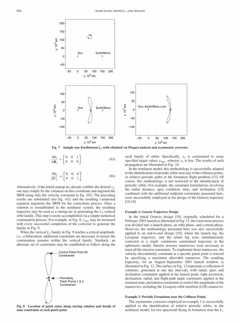
The two short-period modes may also be combined to generategenerally three-dimensional orbits. However, to ensure that thegeometry of the startup arc is preserved during the correctionsprocess, additional interior constraints may be necessary. Tobetter illustrate this, consider the sample startup solution inFig. 7.

From the solution in Fig. 7, five patch points are selected for thedifferential corrections process, as depicted in Fig. 8. The initial andterminal patch states are arbitrarily selected along the orbit and arelabeled as points one and five. To preserve the overall features of thisorbit during the corrections process, control points are strategicallyintroduced at the second and fourth patch states, where the orbitachieves extremal values in the z component. For instance, let zkdesrepresent the desired value of the z component at the kth patch state,for k� 2.

In addition to the periodicity constraint, implemented at patchstates one and five, the corrector matrix is also augmented toincorporate the following constraints [24]:

� 2 �z2 � z2des

_z2

� �(92)

The nonzero constraint partials, associated with Eq. (92), are definedas

−60 −40 −20 0 20 40 60−60

−40

−20

0

20

40

60

L4

x, 106 km

y, 1

06 k

m

λ3,4

−60 −40 −20 0 20 40 60−60

−40

−20

0

20

40

60

L4

x, 106 km

z, 1

06 k

m

Fig. 5 Linearized long-period natural motion near L4.

−50 0 50 100 150 200

−50

0

50

100

150

200

Earth/Moon

x, 106 km

Sun

y, 1

06 k

m

−50 0 50 100 150 200

−100

−50

0

50

100

Earth/Moon

x, 106 km

Sun

z, 1

06 k

m

−50 0 50 100 150 200

−100

−50

0

50

100

y, 106 km

Sun−Earth/Moon Line

z, 1

06 k

m

Fig. 6 Converged vertical orbit near L4, determined in the nonlinear CR3BP.


@�2

@R2

� 0 0 1

0 0 0

� �(93)

@�2

@V2� 0 0 0

0 0 1

� �(94)

Alternatively, if the initial startup arc already exhibits the desired z2,one may simply fix the variation on this coordinate and augment theSRM using only the velocity constraint in Eq. (92). The precedingresults are substituted into Eq. (42) and the resulting variationalequation augments the SRM for the corrections process. Once asolution is reestablished in the nonlinear system, the resultingtrajectory may be used as a startup arc in generating the L4 verticalorbit family. This step is easily accomplished via a simple numericalcontinuation process. For example, in Fig. 8, z2des may be increasedwith every successful completion of the corrector to generate thefamily in Fig. 9.

When the vertical L4 family in Fig. 9 reaches a critical amplitude,i.e., a bifurcation, additional constraints are necessary to ensure thecontinuation remains within the vertical family. Similarly, analternate set of constraints may be established to follow along the

axial family of orbits. Specifically, x2 is constrained to somespecified target values x2des, whereas z2 is free. The results of suchpropagation are illustrated in Fig. 10.

In the nonlinear model, this methodology is successfully adaptedto the identification of periodic orbits near any of the collinear points,or relative periodic paths in the formation flight problem [13]. Ofcourse, this methodology is not restricted to the identification ofperiodic orbits. For example, the constraint formulations involvingthe radial distance, apse condition, time, and inclination [10]combined with the additional endpoint constraints presented here,were successfully employed in the design of the Genesis trajectory[18,19].

Example 2: Genesis Trajectory Design

In the initial Genesis design [18], originally scheduled for aFebruary 2001 launch as illustrated in Fig. 11, the corrections processwas divided into a launch phase, an orbit phase, and a return phase.However, the methodology presented here was also successfullyapplied to an end-to-end design [19], where the launch leg, theLissajous trajectory, and the return leg were simultaneouslycorrected as a single continuous constrained trajectory in theephemeris model. Interior nonzero maneuvers were necessary tomeet all the mission constraints. To implement these maneuvers, thevelocity discontinuity constraint at a specific patch point is relaxedby specifying a maximum allowable maneuver. The resultingtrajectory, for an August–September 2001 launch window, isillustrated in Fig. 12. The surface in Fig. 12 represents a collection ofsolutions, generated at one day intervals, with radial, apse, andinclination constraints applied at the launch point, right ascension,declination, radial, and flight-path angle constraints applied at theterminal state, and interior constraints to restrict the magnitude of themaneuvers, including the Lissajous orbit insertion (LOI) maneuver.

Example 3: Periodic Formations near the Collinear Points

The asymmetric corrector employed in example 1 is successfullyapplied to the identification of relative periodic orbits, in thenonlinear model, for two spacecraft flying in formation near the L1

−50 0 50 100 150 200

−50

0

50

100

150

200

Earth/Moon

x, 106 km

Suny,

10

6 km

−50 0 50 100 150 200

−100

−50

0

50

100

Earth/Moon

x, 106 km

Sun

z, 1

06 k

m

−50 0 50 100 150 200

−100

−50

0

50

100

y, 106 km

Sun−Earth/Moon Line

z, 1

06 k

m

Fig. 7 Sample sun–Earth/moon L4 orbit obtained via Floquet analysis and asymmetric corrector.

Control Patch Point #2Constrained

PeriodicityPatch Points 1 & 5Constrained

Fig. 8 Location of patch states along startup solution and details of

state constraints at each patch point.


andL2 libration points. Howell andMarchand [13] identify a numberof periodic and slowly drifting relative orbits for two spacecraftflying in formation in the vicinity of an L1=L2 halo orbit. Theidentification of the startup arcs is, once again, facilitated by aFloquet approach [13]. The process of transitioning these periodic

arcs into the nonlinear model is accomplished through the use of theasymmetric corrector discussed here. Figure 13 illustrates anexample where the initial arc is closed through the addition ofnonzero impulsive maneuvers at two points along the trajectory.Within one or two iterations, the asymmetric corrector quickly

−50 0 50 100 150 200

−50

0

50

100

150

200

x, 106 km

y, 1

06 k

m

−50 0 50 100 150 200

−100

−50

0

50

100

x, 106 km

z, 1

06 k

m

−50 0 50 100 150 200

−100

−50

0

50

100

y, 106 km

z, 1

06 k

m

Earth/MoonSun

Earth/MoonSun Sun−Earth/Moon Line

Fig. 9 Neighboring L4 family of orbits obtained by varying the terminal z value in the asymmetric corrector.

−50 0 50 100 150 200

−50

0

50

100

150

200

x, 106 km

y, 1

06 k

m

−50 0 50 100 150 200

−100

−50

0

50

100

x, 106 km

z, 1

06 k

m

−50 0 50 100 150 200

−100

−50

0

50

100

y, 106 km

z, 1

06 k

m

Earth/MoonSun

Earth/MoonSunSun−Earth/Moon Line

Fig. 10 Results of arbitrary L4 family propagation along y axis.


identifies the neighboring periodic arc and drives the initialmaneuvers to zero.

Conclusions

In this investigation, an asymmetric constrained differentialcorrector is presented. An immediate advantage of this approach,particularly for the identification of periodic orbits, is that the startuparc need not exhibit any symmetry for the methodology to achievethe formulated objectives or satisfy the imposed interior and exteriorconstraints. The versatility and generality of the two-levelconstrained differential corrector is demonstrated through threedistinct examples: the identification of asymmetric periodic orbitsnear the triangular points, the end-to-end constrained design of theGenesis trajectory, and the identification of periodic relative arcs inthe formation flight problem.

For autonomous dynamic systems, the methodology is suc-cessfully applied to the identification of trajectory arcs subject toalgebraic constraints, periodic orbits, quasi-periodic trajectories,

or combinations thereof. It is important to note that the processis in no way exclusive to the gravitational n-body problem orspacecraft mission design. If the dynamic system is autonomous,the constraints can be specified algebraically, and the constraintderivatives exist, the methodology is easily adapted to a varietyof applications. For spacecraft mission design, however, theresults of this investigation demonstrate that the asymmetricconstrained differential corrector is able to minimize velocitydiscontinuities and enforce constraints in a cohesive manner, andproves to be an efficient end-to-end design tool.

Acknowledgments

The authors extend their appreciation to Daniel Grebow, fromPurdue University, for his contributions to the implementation ofexample 1. Portions of this work were completed at PurdueUniversity and the Jet Propulsion Laboratory, California Institute ofTechnology under contract with NASA.

Fig. 11 Initial Genesis trajectory design (courtesy NASA/JPL-Caltech).

Fig. 12 Genesis summer 2001 launch options.


References

[1] Poincaré, H., New Methods of Celestial Mechanics, Vol. 1, AmericanInst. of Physics, New York, 1993; also Periodic and AsymptoticSolutions, Translated from the French, Revised Reprint of the 1967English Translation, with Endnotes by V. I. Arnold, Edited and with anIntroduction by D. L. Goroff.

[2] Farquhar, R. W., Muhonen, D. P., Newman, C. R., and Heuberger, H.S., “Trajectories and Orbital Maneuvers for the First Libration-PointSatellite,” Journal of Guidance and Control, Vol. 3, No. 6, 1980,pp. 549–554.

[3] Farquhar, R. W., “Flight of ISEE-3/ICE: Origins, Mission History, anda Legacy,” Journal of the Astronautical Sciences, Vol. 49, No. 1, 2001,pp. 23–73.

[4] Dunham, D.W., Jen, S. J., Roberts, C. E., Seacord, A.W., II, Sharer, P.J., Folta, D. C., and Muhonen, D. P., “Double Lunar-SwingbyTrajectories for the Spacecraft of the International Solar-TerrestrialPhysics Program,” Orbital Mechanics and Mission Design: Advances

in the Astronautical Sciences, AAS/NASA International Symposium,Vol. 69, American Astronautical Society, 1989, pp. 285–301.

[5] Dunham, D.W., Jen, S. J., Roberts, C. E., Seacord, A.W., II, Sharer, P.J., Folta, D. C., andMuhonen,D. P., “Transfer TrajectoryDesign for theSOHO Libration-Point Mission,” 43rd International Astronautical

Congress, Washington, International Astronautical FederationPaper 92-0066, 1992.

[6] Stone, E. C., Frandsen, A. M., Mewaldt, R. A., Christian, E. R.,Margolies, D., Ormes, J. F., and Snow, F., “Advanced CompositionExplorer,” Space Science Reviews, Vol. 86, Nos. 1–4, 1998, pp. 1–22.

[7] Cuevas, O., Kraft-Newman, L., Mesearch, M., and Woodard, M.,“Overview of Trajectory Design Operations for the MicrowaveAnisotropy Probe Mission,” AIAA/AAS Astrodynamics Specialist

Conference and Exhibit, AIAA Paper 2002-4425, 2002.[8] Lo,M.,Williams, B., Bollman,W.,Han,D., Hahn,Y., Bell, J., Hirst, E.,

Corwin, R., Hong, P., Howell, K. C., Barden, B., and Wilson, R.,“GENESIS Mission Design,” Journal of the Astronautical Sciences,Vol. 49, No. 1, 2001, pp. 169–184.

[9] Wilson, R. S., “Trajectory Design in the Sun-Earth-Moon Four BodyProblem,” Ph.D. Dissertation, School of Aeronautics and Astronautics,Purdue Univ., West Lafayette, IN, 1998.

[10] Wilson, R. S., and Howell, K. C., “Trajectory Design in the Sun-Earth-Moon SystemUsing Lunar Gravity Assists,” Journal of Spacecraft andRockets, Vol. 35, No. 2, 1998, pp. 191–198.

[11] Howell, K. C., “Three-Dimensional Periodic Halo Orbits,” Celestial

Mechanics, Vol. 32, No. 1, 1984, pp. 53–71.[12] Markellos, V. V., “Three-Dimensional General Three-Body Problem:

Determination of Periodic Orbits,”CelestialMechanics, Vol. 21, No. 3,1980, pp. 291–309.

[13] Howell, K. C., and Marchand, B. G., “Natural and Non-Natural

Spacecraft Formations Near the L1 and L2 Libration Points in the Sun-Earth/Moon Ephemeris System,,” Dynamical Systems: an Interna-

tional Journal, Special Issue “Dynamical Systems in DynamicalAstronomy and Space Mission Design, Vol. 20, No. 1, 2005, pp. 149–173.

[14] Richardson, D. L., “Analytic Construction of Periodic Orbits About theCollinear Points,” Celestial Mechanics, Vol. 22, No. 3, 1980, pp. 241–253.

[15] Richardson, D. L., and Cary, N. D., “Uniformly Valid Solution forMotion about the Interior Libration Point of the Perturbed Elliptic-Restricted Problem,” AAS/AIAA Astrodynamics Specialists Confer-

ence, American Astronautical Society Paper 75-021, 1975.[16] Howell, K. C., Marchand, B. G., and Lo, M. W., “Temporary Satellite

Capture of Short-Period Jupiter Family Comets from the Perspective ofDynamical Systems,” Journal of the Astronautical Sciences, Vol. 49,No. 4, 2001, pp. 539–557.

[17] Howell, K. C., and Pernicka, H. J., “Numerical Determination ofLissajous Trajectories in the Restricted Three-Body Problem,”Celestial Mechanics, Vol. 41, Nos. 1–4, 1987, pp. 107–124.

[18] Howell, K. C., Barden, B. T.,Wilson, R. S., and Lo,M.W., “TrajectoryDesign Using a Dynamical Systems Approach with Application toGENESIS,” AAS/AIAA Astrodynamics Conference, Sun Valley, Idaho,American Astronautical Society Paper 97-7091997, pp. 1665–1684.

[19] Wilson, R. S., Barden, B. T., Howell, K. C., and Marchand, B. G.,“Summer Launch Options for the Genesis Mission,” Advances in the

Astronautical Sciences, Vol. 109, Part 1, 2002, pp. 77–94.[20] Markellos, V. V., and Halioulias, A. A., “Numerical Determination of

Asymmetric Periodic Solutions,” Astrophysics and Space Science,Vol. 46, No. 1, 1977, pp. 183–193.

[21] Zagouras, C. G., “Three Dimensional Periodic Orbits about theTriangular Equilibrium Points of the Restricted Problem of ThreeBodies,” Celestial Mechanics, Vol. 37, No. 1, 1985, pp. 27–46.

[22] Papadakis, K. E., and Zagouras, C. G., “Bifurcation Points andIntersections of Families of Periodic Orbits in the Three-DimensionalRestricted Three-Body Problem,” Astrophysics and Space Science,Vol. 199, No. 2, 1993, pp. 241–256.

[23] Zagouras, C. G., Perdois, E., and Ragos, O., “New Kinds ofAsymmetric Periodic Orbits in the Restricted Three-Body Problem,”Astrophysics and Space Science, Vol. 240, No. 2, 1996, pp. 273–293.

[24] Grebow, D. J., “Generating Periodic Orbits in the Circular RestrictedThree-bodyProblemwithApplications toLunar South PoleCoverage,”M.S. Thesis, School of Aeronautics and Astronautics, Purdue Univ.,West Lafayette, IN, 2006.

C. KlueverAssociate Editor

Fig. 13 Periodic relative path near a spacecraft evolving along an L2 halo orbit.


improved corrections process for constrained trajectory

Documents