improved approach to lidar airport obstruction …nowak.ece.wisc.edu/lidar08.pdf · improved...
TRANSCRIPT
1
Improved Approach to Lidar Airport Obstruction Surveying Using Full-
Waveform Data
Christopher E. Parrish1 and Robert D. Nowak
2
ABSTRACT
Over the past decade, the National Oceanic and Atmospheric Administration’s National Geodetic
Survey, in collaboration with multiple organizations, has conducted research into airport
obstruction surveying using airborne lidar. What was initially envisioned as a relatively
straightforward demonstration of the utility of this emerging remote sensing technology for
airport surveys was quickly shown to be a challenging undertaking fraught with both technical
and practical issues. We provide a brief history of previous work in lidar airport obstruction
surveying, including a discussion of both past achievements and previously-unsolved problems.
We then present a new processing workflow, specifically designed to overcome the remaining
problems. A key facet of our approach is the use of a new lidar waveform deconvolution and
georeferencing strategy that produces very dense, detailed point clouds in which the vertical
structures of objects are well characterized. Additional processing steps have been carefully
selected and ordered based on the objectives of meeting Federal Aviation Administration
requirements and maximizing efficiency. Tests conducted using lidar waveform data for two
project sites demonstrate the efficacy of the approach.
1 Physical Scientist, NOAA, National Geodetic Survey, 1315 East-West Highway, Silver Spring, MD 20910 2 McFarland-Bascom Professor in Engineering, University of Wisconsin-Madison, Department of Electrical and Computer Engineering, 2420 Engineering Hall, Madison, WI 53706

2
CE Database subject headings: Aerial surveys, Air transportation, Airports, Lasers, Mapping
Introduction
Airport obstruction surveys enhance the safety of the National Airspace System (NAS) by
providing accurate spatial coordinates for objects that could potentially pose hazards to aircraft
on takeoff and landing. By definition, an obstruction is any natural or manmade object, such as a
tree, tower, antenna, or building that penetrates an airport’s obstruction identification surfaces
(OIS) (FAA 1996; FAA 2008). The OIS are mathematically-defined, imaginary 3D surfaces that
typically encompass the airfield and approaches. The data are used by the Federal Aviation
Administration (FAA) in designing runway approach procedures and also serve a wide variety of
other applications, ranging from determining takeoff weights to certifying airports for certain
types of operations, to conducting airport planning studies (FAA 1996; FAA 2008).
Conventional methods of airport obstruction surveying comprise a combination of
photogrammetric and field survey techniques (Pates 1950; Smith 1981; Tuell 1987; FAA 1996),
and these methods have been proven over the past half century and thousands of surveys to yield
very accurate, reliable obstruction data. However, the desire to increase efficiency and reduce
costs in airport obstruction surveying has led to increasing interest in airborne light detection and
ranging (lidar) for this application. In one early study into the applicability of airborne lidar in
airport obstruction surveying (Uddin and Al-Turk 2002), several potential benefits of lidar were
identified, including cost and time savings.
One of the first studies to empirically assess the capability to meet FAA specifications for
obstruction surveying using lidar was conducted jointly by the National Geodetic Survey (NGS),
the FAA, University of Florida, and Optech, Inc. in 2001 (Anderson et al. 2002). Data were
3
acquired for approaches to Gainesville Regional Airport (GNV) using commercial airborne lidar
systems with standard topographic mapping configurations and compared against field-surveyed
reference data. Although several field-surveyed obstructions, such as poles and antennas, were
missed in the lidar surveys, the study yielded the following important conclusions (Anderson et
al. 2002; Parrish 2003):
(1) The limiting factor in the ability to meet FAA specifications for obstruction data with
lidar is not the accuracy with which laser returns can be geolocated. Rather, the primary
factors are the ability to achieve sufficient horizontal and vertical point density and
sufficient received signal strength to detect the tops of small-diameter, low-reflectance
objects, such as poles and antennas.
(2) The typical system configurations and data acquisition and processing parameters used
for topographic mapping (i.e., generation of bare-earth terrain data sets) are poorly suited
for airport obstruction surveying.
These conclusions motivated a second phase of research, in which the capability to improve
obstruction detection results through appropriate selection of the system settings and data
acquisition and processing parameters was investigated (Parrish et al. 2005). The data
acquisition included flights using fourteen different configurations, consisting of different
settings and combinations of forward tilt angle, beam divergence, and flying height. The two
best configurations resulted in 100% detection of the field-surveyed objects at GNV. A third
phase of NGS’ research into lidar airport obstruction surveying was then carried out in 2003 to
investigate the capability to conduct a complete end-to-end obstruction survey using lidar
(Parrish et al. 2004). Data were acquired using a dual lidar system (one sensor head at nadir and
the other configured with a 20o forward tilt angle) for Frederick Municipal Airport (FDK) and
4
Stafford Regional Airport (RMN). A noteworthy outcome of this work was the development by
the FAA of the first instrument approach procedure in the U.S. based on a lidar survey (Fred
Anderson, internal FAA report, 2004).
While the above-mentioned studies made great strides towards demonstrating the technical
feasibility of lidar obstruction surveys, the issue of practicality remained largely unaddressed. A
major challenge in performing lidar obstruction surveys efficiently and cost effectively stems
from the fact that, although the FAA is migrating towards acceptance of survey data in a variety
of Geographic Information System (GIS) compatible formats (FAA 2008), the current
operational workflow and software used by FAA approach procedure developers are not
designed to work with raw lidar point clouds. Rather, they require obstruction data in the form
of discrete obstacle lists containing coordinate information and feature names for individual
objects (e.g., trees, poles, buildings, etc.) in text-based Universal Data Delivery Format (UDDF)
files (FAA 2007; FAA 1996). Creating these final UDDF obstruction lists from the raw point
cloud is a non-trivial task. Using NGS surface modeling software, it is possible to analyze the
raw lidar point cloud against the OIS and extract penetrating lidar points (Parrish et al. 2004).
However, the removal of non-penetrating lidar points complicates all of the following tasks:
(1) distinguishing between returns from actual objects and those due to noise or clutter;
(2) determining which points correspond to returns from the same object; and
(3) attributing detected obstructions.
Hence, previous NGS lidar airport obstruction surveys required a great deal of manual analysis,
largely negating the intended cost and time savings. An independent study by Wang et al. (2004)
described a workflow for lidar airport surveying based on National Geospatial-Intelligence
Agency (NGA, formerly the National Imagery and Mapping Agency) requirements. As in the

5
NGS studies, the end process was fairly complicated, containing approximately 20 steps and
relying on aerial imagery and topographic maps.
In this paper we describe a new workflow for lidar airport obstruction surveying that
addresses the problems described above. Two important aspects of our approach are the
utilization of the additional information contained in full-waveform lidar data to enhance vertical
object (VO) detection and the sequencing of steps in the workflow to improve both the efficiency
and end results. Experiments conducted using lidar waveform data collected for two project sites
in Madison, Wisconsin, are described, followed by the results and conclusions.
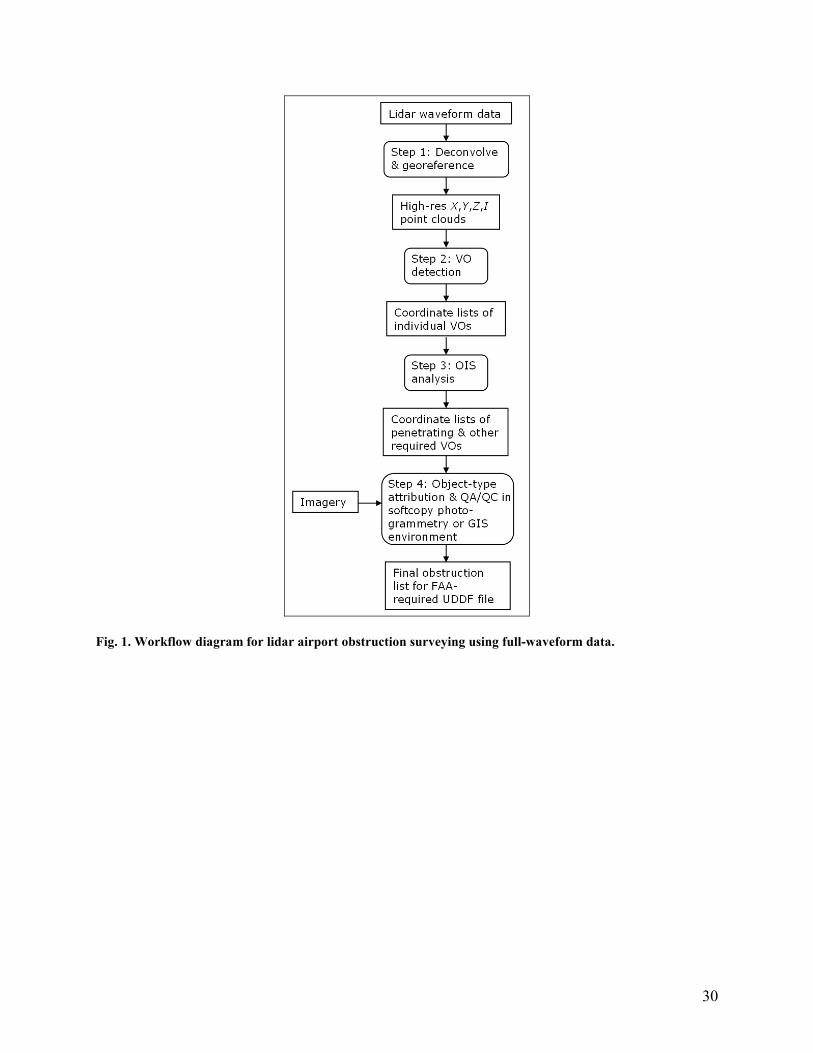
Proposed Workflow for Lidar Airport Obstruction Surveying
The lidar airport obstruction surveying workflow developed and tested in this research is
illustrated in Fig. 1. This workflow has been specifically designed and ordered to form an
efficient practical methodology for lidar obstruction surveying, while simultaneously improving
the capability to meet FAA obstruction surveying standards. As shown in the figure, it
comprises four steps, with the input consisting of full-waveform lidar data (which will be further
described below) and aerial imagery, preferably, but not necessarily, collected concurrently. The
output consists of final obstruction lists in the FAA-specified format. Advantages of this
workflow can be summarized as follows:
• Utilizes the additional information contained in full-waveform lidar to improve object
detection.
• Minimizes the probability of a missed obstruction, because the detection threshold in the
object extraction step can be set very conservatively, and false alarms can be easily
(usually automatically) eliminated in the subsequent processing steps.
6
• Facilitates creation of the final FAA-required obstruction lists by placing the object
extraction step as early in the process as possible and ensuring that all following steps
operate on objects, not points.
• Increases efficiency by combining all steps that require manual analysis.
• Requires only four steps for generation of the final deliverables to the FAA (i.e.,
obstruction information in UDDF format).
Two assumptions are made regarding the input data: first, the airborne data acquisition has
been performed using the recommended mission parameters and system settings contained in
NGS (2004) and Parrish et al. (2005); second, the lidar data include digitized waveforms.
Waveform digitization is a relatively new advancement in commercially-available airborne lidar
systems (e.g., Hug et al. 2004; Gutierrez et al. 2005). Unlike earlier discrete-return systems that
only recorded a small number of returns (e.g., one to four) per transmitted pulse, full-waveform
systems are capable of digitizing the entire received signal from each transmitted pulse at very
high sampling frequencies (e.g., 1 GHz), often producing a few hundred samples per return.
Full-waveform systems overcome the “minimum pulse separation limitation” of discrete-return
systems (i.e., the inability to resolve features separated by less than a few meters in the range
direction), which results from the inevitable limitations of the rangefinder electronics
(Nayegandhi et al. 2006; Optech 2006).
To clarify the above statements and more fully describe the workflow, the following is a
detailed, step-by-step description of the process:
7
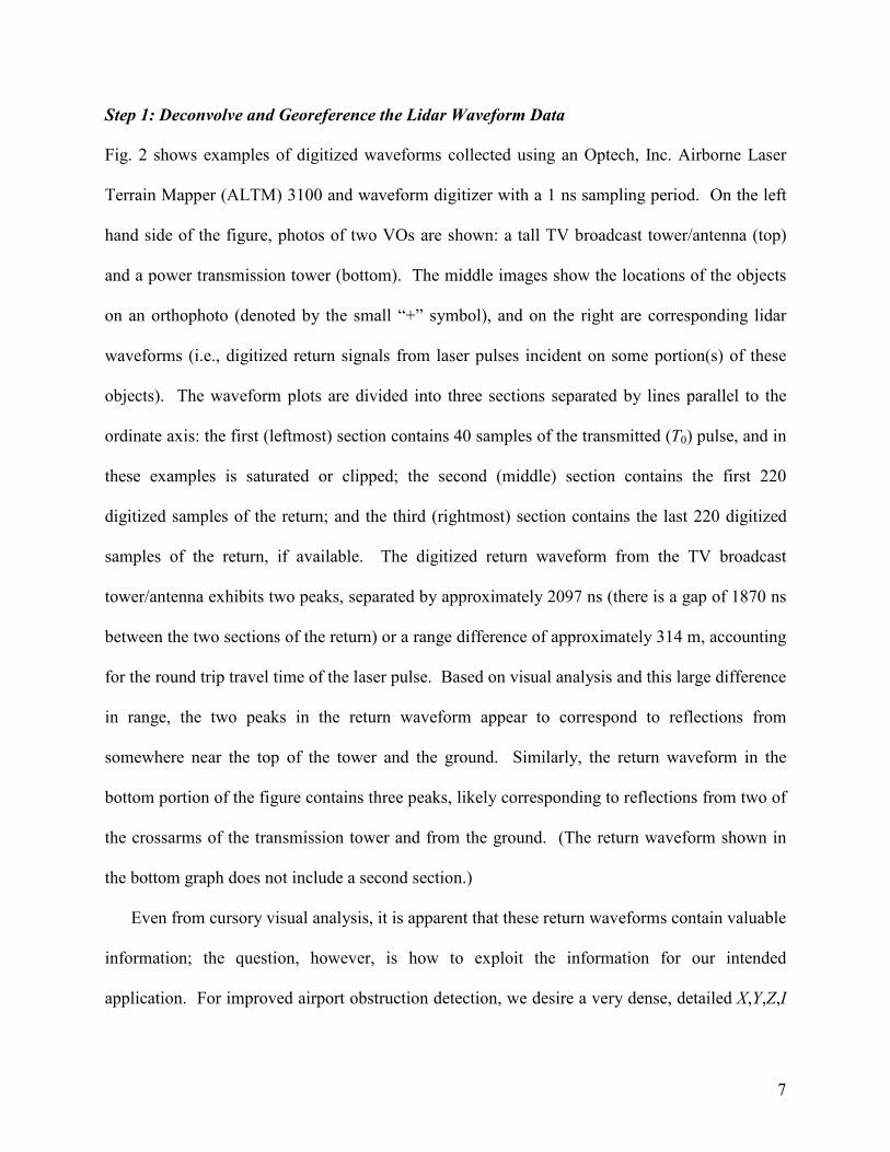
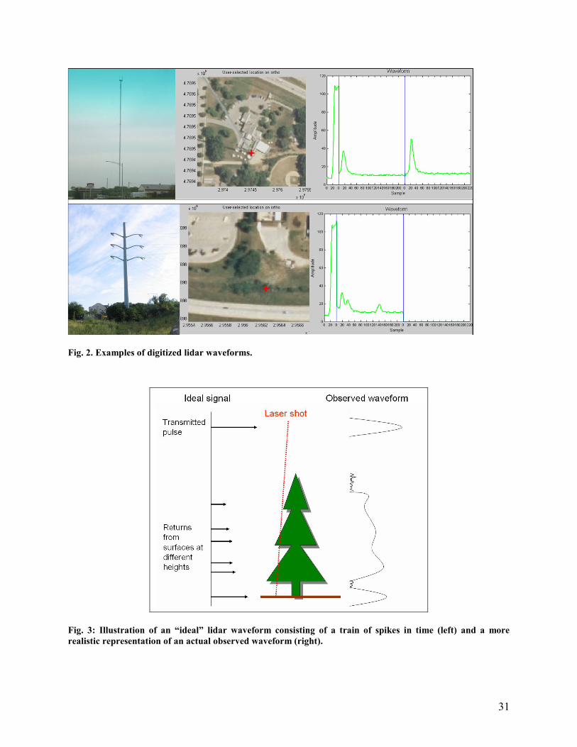
Step 1: Deconvolve and Georeference the Lidar Waveform Data
Fig. 2 shows examples of digitized waveforms collected using an Optech, Inc. Airborne Laser
Terrain Mapper (ALTM) 3100 and waveform digitizer with a 1 ns sampling period. On the left
hand side of the figure, photos of two VOs are shown: a tall TV broadcast tower/antenna (top)
and a power transmission tower (bottom). The middle images show the locations of the objects
on an orthophoto (denoted by the small “+” symbol), and on the right are corresponding lidar
waveforms (i.e., digitized return signals from laser pulses incident on some portion(s) of these
objects). The waveform plots are divided into three sections separated by lines parallel to the
ordinate axis: the first (leftmost) section contains 40 samples of the transmitted (T0) pulse, and in
these examples is saturated or clipped; the second (middle) section contains the first 220
digitized samples of the return; and the third (rightmost) section contains the last 220 digitized
samples of the return, if available. The digitized return waveform from the TV broadcast
tower/antenna exhibits two peaks, separated by approximately 2097 ns (there is a gap of 1870 ns
between the two sections of the return) or a range difference of approximately 314 m, accounting
for the round trip travel time of the laser pulse. Based on visual analysis and this large difference
in range, the two peaks in the return waveform appear to correspond to reflections from
somewhere near the top of the tower and the ground. Similarly, the return waveform in the
bottom portion of the figure contains three peaks, likely corresponding to reflections from two of
the crossarms of the transmission tower and from the ground. (The return waveform shown in
the bottom graph does not include a second section.)
Even from cursory visual analysis, it is apparent that these return waveforms contain valuable
information; the question, however, is how to exploit the information for our intended
application. For improved airport obstruction detection, we desire a very dense, detailed X,Y,Z,I

8
lidar point cloud (where X, Y, and Z are spatial coordinates, and I denotes intensity), in which the
vertical structures of objects are well characterized. Each individual laser reflection should map
to a point in the point cloud and the intensity value of the point should be proportional to the
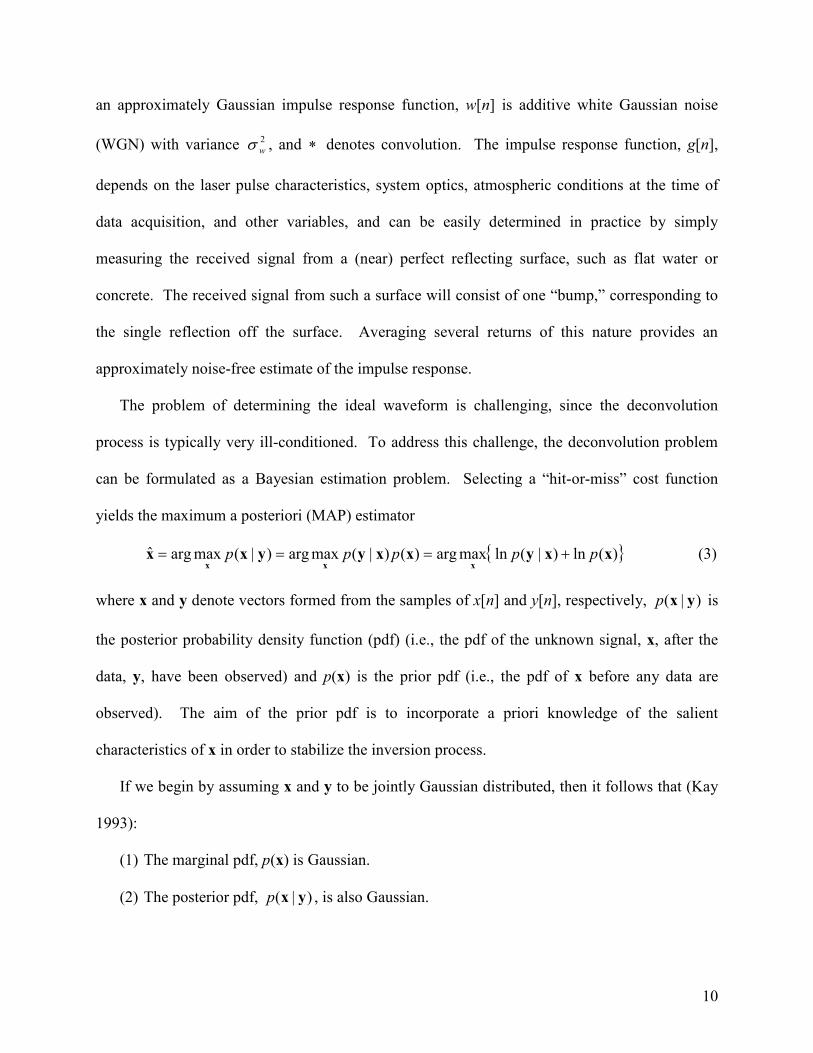
amount of backscattered energy. The process of generating this point cloud would be trivial if
we were to start with a set of “ideal” waveforms, as depicted on the left-hand side of Fig. 3. This
ideal waveform consists of a train of spikes in time, where each spike corresponds to an
individual laser reflection, with its amplitude being proportional to the strength of the return and
its position on the time axis being proportional to the range. For example, in a forested area, the
first spike in a particular idealized return might correspond to a reflection from the top-most
branch or leaf in a tree, while the second spike might correspond to a reflection from the next
lower branch, and so on down to the ground.
An actual received waveform, as depicted on the right-hand side of Fig. 3, can be considered
a blurry, noisy version of the ideal waveform. One method of estimating the desired parameters
(e.g., individual ranges and amplitudes) from the observed waveform is through a process called
Gaussian decomposition, originally proposed as a processing strategy for data from the large-
footprint, NASA-owned-and-operated Laser Vegetation Imaging Sensor (LVIS) system (Hofton
et al. 2000) and recently applied to data from some of the very early commercial, small-footprint,
full-waveform systems (e.g., Persson et al. 2005; Reitberger et al. 2006; Wagner et al. 2006). In
this approach, each received waveform is modeled as a convex combination of K Gaussian
density functions (i.e., a K-component Gaussian mixture model), or
( )∑=
−−=K
i
i
i
i tty1
2
22
1exp)(ˆ µ
σα (1)
where αi is the amplitude of the ith component, σi is its standard deviation, and µi is its mean.
The objective is to obtain statistically optimal estimates (based on some defined optimality

9
criterion) of the unknown parameters {αi, σi, µi} for K components, where K can be adjusted
until the fit of the model to the data is within some prescribed tolerance. A preprocessing step of
denoising by lowpass filtering is typically employed.
While some studies have demonstrated quite good results using Gaussian decomposition
(e.g., Reitberger et al. 2006; Persson et al. 2005), in this research, we investigated a
deconvolution approach. Although deconvolution of airborne lidar waveforms has received
comparatively little attention in the literature to date (Nordin 2006; Walter 2005), the devolution
strategy investigated in this work offers the following advantages over the Gaussian
decomposition approach:
(1) The algorithm is robust against local minima problems and, with slight modification to
the thresholding step that will be described below (i.e., through use of a soft threshold)
guarantees convergence to the globally-optimal solution.
(2) The issue of noise in the data is addressed directly, rather than with an ad hoc
preprocessing step.
(3) The inverse problem is solved, rather than attempting to directly fit the return waveform
data.
(4) The computational costs are low.
Specifically, we employed the Expectation Maximization (EM) deconvolution strategy of
Figueiredo and Nowak (2003), also referred to in the literature as an iterative
shrinkage/thresholding (IST) algorithm. We start with the following observation model
][][][][ nwnxngny +∗= (2)
where x[n] is the ideal/undegraded (discrete-time) signal illustrated graphically on the left hand
side of Fig. 3, y[n] is the observed waveform depicted on the right hand side of the figure, g[n] is
10
an approximately Gaussian impulse response function, w[n] is additive white Gaussian noise
(WGN) with variance 2wσ , and ∗ denotes convolution. The impulse response function, g[n],
depends on the laser pulse characteristics, system optics, atmospheric conditions at the time of
data acquisition, and other variables, and can be easily determined in practice by simply
measuring the received signal from a (near) perfect reflecting surface, such as flat water or
concrete. The received signal from such a surface will consist of one “bump,” corresponding to
the single reflection off the surface. Averaging several returns of this nature provides an
approximately noise-free estimate of the impulse response.
The problem of determining the ideal waveform is challenging, since the deconvolution
process is typically very ill-conditioned. To address this challenge, the deconvolution problem
can be formulated as a Bayesian estimation problem. Selecting a “hit-or-miss” cost function
yields the maximum a posteriori (MAP) estimator
{ })(ln)|(lnmaxarg)()|(maxarg)|(maxargˆ xxyxxyyxxxxx
ppppp +=== (3)
where x and y denote vectors formed from the samples of x[n] and y[n], respectively, )|( yxp is
the posterior probability density function (pdf) (i.e., the pdf of the unknown signal, x, after the
data, y, have been observed) and p(x) is the prior pdf (i.e., the pdf of x before any data are
observed). The aim of the prior pdf is to incorporate a priori knowledge of the salient
characteristics of x in order to stabilize the inversion process.
If we begin by assuming x and y to be jointly Gaussian distributed, then it follows that (Kay
1993):
(1) The marginal pdf, p(x) is Gaussian.
(2) The posterior pdf, )|( yxp , is also Gaussian.
11
(3) The MAP estimator and minimum mean square error (MMSE) estimator are the same,
since the mean and mode (location of the maximum) of a Gaussian are identical.
In this case, the MAP estimator is equivalent to the well-known Wiener filter (linear MMSE
estimator). (As an aside, Wiener filtering as a strategy for lidar waveform processing was
discussed in Jutzi and Stilla (2006), although in that work it was utilized primarily as a denoising
step preceding Gaussian decomposition of the signal.)
While the Wiener filter is a commonly-used approach for signal/image restoration, it suffers
some serious drawbacks for this particular application. Specifically, the prior pdf assumed in the
Wiener filter essentially models the signal, x, as a white Gaussian noise process with a certain
power, 2xσ , and does not reflect prior knowledge about the structure of the waveforms. However,
based on the physics of the problem, we know our signals are not arbitrary, noise-like
waveforms; rather they are much better modeled as trains of spikes in time, with each spike
corresponding to an individual laser reflection (c.f. Fig. 3). The advantage of the approach
developed by Figueiredo and Nowak (2003) is that it solves for the MAP estimate (Eq. (3)) while
allowing us to incorporate knowledge of the waveform structure through selection of the prior
pdf. The prior pdf employed here models the ideal waveforms as random spike trains, and is
essentially determined by specifying the probability, p, of observing a spike at each point in time.
In this model, each time point is treated as statistically independent of all other time points (i.e.,
the probability of a spike at one time point is independent of all other time points). This prior
pdf is quite different from the Gaussian white noise pdf implicit in the Wiener filter. Because a
closed form solution for the MAP estimator does not exist, it is computed numerically, iterating
between a partial deconvolution step (the E-step) and a thresholding step (M-Step), which, in our
implementation, can be expressed in the time domain as

12
( )( ){ }
][ˆ
0,][ˆmax][ˆ :step-M
][ˆ][][][][ˆ][ˆ :step-E
)(
22)()1(
)()()(
nz
nznx
nxngnyngnxnz
t
w
tt
ttt
τσ−=
∗−∗+=
+
∗
(4)
In Eq. (4), ][ˆ )( nx t is the estimate of the signal x[n] at the tth iteration of the algorithm; ][ˆ )( nz t is
the estimate of the missing data in the EM procedure (as explained in Figueiredo and Nowak
2001, 2003; Nowak and Figueiredo 2001); g[n] is the impulse response function, estimated as
described above; and, at the implementation level, the nonnegative parameter τ can be
considered a tunable parameter controlling the number of spikes in the output. In particular, τ
can be inversely related to the prior probability of a spike at a given location. The specific form
of the denoising M-step in Eq. (4) results from the selection of the prior described in Figueiredo
and Nowak (2003). The procedure above is iterated until convergence, which can be declared
using any number of reasonable stopping criteria, such as stopping when the relative difference
between successive iterations is less than a specified tolerance of 10-3. It is important to note that
each iteration can be rapidly computed. The E-Step requires two convolutions with the impulse
response function. This can be computed in N log N operations (where N is the number of
samples in the received signal) using the Fast Fourier Transform (FFT). The M-Step applies a
scalar thresholding operation to each element of the output of the E-Step, and hence requires
only N operations. Thus, the overall computational complexity of each iteration is O(N log N),
roughly the same complexity as the Wiener filter.
Fig. 4 shows examples of deconvolving two actual lidar waveforms (top, green) using the
EM deconvolution algorithm (bottom, red) and, for comparison, a Wiener filter (middle, blue).
From these examples, the superiority of the EM deconvolution algorithm in this application is
clear: the output signals are much sharper (in fact, we have produced the desired train of spikes
in time), and the noise has been completely suppressed. Additionally, the EM deconvolution
13
algorithm output does not contain the ringing (artificial oscillations around sharp edges) evident
in the Wiener-filtered waveforms—especially important, since, if the Wiener-filtered waveforms
are subsequently georeferenced, the ringing artifacts carry over into the output point clouds
(Parrish 2007a).
Since the location on the time axis of each spike in the graphs on the bottom portion of Fig. 4
is proportional to the range, and since the post-processed Global Positioning System/Inertial
Measurement Unit (GPS/IMU) and scanner angle data are presumably already available through
the standard processing, point clouds can be generated at this point through straightforward
application of the laser geolocation equation (e.g., Vaughn et al. 1996; Filin 2001). The
amplitude of each spike is the value assigned to the intensity of the corresponding point in the
output point cloud.
An extremely attractive feature of this EM deconvolution algorithm is provision of the
tunable parameter τ, capable of being adjusted based on the considerations of the particular end-
user application. Decreasing τ has the effect of increasing the number of spikes in the output
(and, hence, the density of the output point clouds), but also increases the probability of “false
spikes”; increasing τ has the opposite effect. For our application of airport obstruction
surveying, it is highly desirable to decrease τ to produce very dense output point clouds to assist
in minimizing the probability of a missed obstruction. The increased probability of “false
objects” output from the next step in the workflow turns out not to be a major concern, since
these false objects can be easily (usually automatically) eliminated in the final two steps, as will
be discussed.

14
Step 2: Detect Vertical Objects (VOs)
The vertical object detection (Step 2) can be performed using any of a number of algorithms or
approaches, including a Hough transform to detect vertical cylinders, cones, and spheres;
morphological filtering algorithms (Woods et al. 2004); a 3D wavelet domain approach (Parrish
2007a,b); or approaches based on eigenvalues of covariance matrices for spherical and
cylindrical environments (Gross et al. 2007). While analysis and comparison of different object
detection strategies is beyond the scope of this paper, two aspects of the detection are of critical
importance in the application of lidar obstruction surveying, regardless of the specific algorithm
utilized: 1) the data model used to store and operate on the lidar data, and 2) the selection of the
detection threshold. Regarding the data model, the primary concern is avoidance of surface
representations, such 2D elevation images/grids, commonly referred to as digital elevation
models (DEMs) or digital surface models (DSMs), or triangulated irregular networks (TINs).
These representations all suffer a serious drawback for our application: namely, it is impossible
to adequately model true vertical surfaces, convex or concave vertical surfaces, and objects
containing multiple, discrete components at the same (X,Y) location but different heights, all of
which leads to severe loss of information about vertical structure (Stoker 2004). For example, it
is impossible to accurately represent roof overhangs, building sidewalls, transmission towers
with multiple crossarms, water towers, and complex-shaped tree canopies. Furthermore, these
surface representations greatly complicate the task of distinguishing between a return from an
actual vertical object, such as a pole, and a return due to noise or clutter (e.g., a bird); in the
elevation image representation both appear as bright pixels (higher elevation) surrounded by
darker pixels (lower elevation). Two suitable alternatives to the use of surface representations

15
are: 1) raw point clouds, or 2) volume, or “voxel,” representations (e.g., Stoker 2004; Vosselman
et al. 2004); the VO detection algorithm should operate on lidar data in one of these formats.
The second consideration is the detection threshold. In signal detection, there are always
tradeoffs between probability of detection, PD, and probability of false alarm, PFA. A common
method of displaying and analyzing the pattern of tradeoffs for a particular detection algorithm is
through the so-called receiver operating characteristic (ROC) curve, a plot of PD versus PFA as
the detector threshold is varied. Although ROC curves vary from detector to detector (and,
therefore, are frequently used in comparing different detection algorithms), there exists a general
trend: decreasing the detector threshold increases both PD and PFA. The sequence of steps in our
workflow has been ordered such that, irrespective of the specific detection algorithm used, the
detection threshold can be set very low to minimize the probability of a miss (or, equivalently,
maximize PD). Object detection is performed first, followed by the OIS analysis, followed by
quality assurance and quality control (QA/QC) and object-type attribution. False alarms (or
“false objects”) due to ground clutter or noise and randomly distributed throughout the project
area will typically be automatically eliminated in the OIS analysis step, due to not penetrating or
falling outside the OIS, and the remainder can be easily removed during the attribution and
QA/QC step. This inherent tolerance of conservative detection thresholds in the object
extraction step is an important aspect of our workflow, since the key consideration in airport
obstruction surveying is to avoid missed obstructions that could potentially jeopardize flight
safety.
16
Step 3: Analyze Detected Objects against OIS
The OIS analysis can be performed easily and quickly using NGS’ Surface Model Library
(SML), a downloadable software library that enables users to mathematically model an airport’s
OIS and perform related analysis (NGS 2008). SML is available as a dynamic-link library
(DLL) that is compatible with Microsoft Visual Basic (VB), C++, and .NET. The library
comprises dozens of functions, which allow users to calculate surface penetrations, analyze
features relative to specified OIS, and numerous other related tasks. NGS is responsible for
updating SML as needed to reflect any changes in the definitions of the OIS (FAA 2008).
Since the implementation is straightforward, the only aspect of this step that merits additional
discussion is its order in the overall workflow; it is critical that the OIS analysis be performed
after, not prior to, the object detection. The reason for this is threefold. First, as already noted,
performing OIS analysis on raw point clouds to extract penetrating points greatly complicates
tasks such as distinguishing between returns from actual objects and noise, grouping returns from
the same object, and performing attribution. Second, this sequence enables the detection
threshold in Step 2 to be set very conservatively (see Step 2 discussion above). Third, since the
final deliverable to the FAA consists of information for obstructions (i.e., objects, not individual
laser reflection locations), it is beneficial to extract objects as early in the process as possible and
to ensure subsequent processing steps operate on those objects.
Step 4: Perform Object-Type Attribution and QA/QC in a Softcopy Photogrammetry or GIS
Environment
While some previous studies have shown that classification (e.g., of tree species) can be
improved using full-waveform data (Reitberger et al. 2006), in airport obstruction surveys, fully-
17
automated classification is arguably an unrealizable objective, because airport obstructions can
include literally any type of natural or manmade object. Fortunately, in this application, manual
attribution can be done without significantly increasing time or cost of the survey, since manual
analysis is already required in the QA/QC step to meet the stringent quality assurance controls.
As shown in previous phases of NGS’ research into lidar obstruction surveying (e.g., Parrish et
al. 2004), this QA/QC is most easily and efficiently performed using stereo imagery in a
softcopy photogrammetry environment, or somewhat less desirably, using orthoimages viewed
monoscopically in a GIS environment. (An advantage of the stereo option is that it enables an
independent check of an object’s top elevation.) By combining of all steps requiring manual
analysis (i.e., attribution and QA/QC), as shown in Step 4 of Fig. 1, an efficient workflow that
minimizes human time is enabled.
Experiment
The workflow described above was tested using airborne and field data for two project sites in
Madison, Wisconsin, as shown in Fig. 5. The airborne data consisted of lidar waveform data
collected with an Optech, Inc. Airborne Laser Terrain Mapper (ALTM) 3100 and waveform
digitizer on June 23-24, 2006, as well as high-resolution digital aerial imagery acquired with an
Applanix, Inc. Digital Sensor System (DSS) 322 on September 14-15, 2006. Received signals
were split in the lidar system, enabling simultaneous acquisition and recording of both discrete-
return and full-waveform data. Mission parameters for the airborne lidar and digital imagery
data acquisition are shown in Tables 1 and 2, respectively. The field data consisted of 35 field-
surveyed reference objects in each of the two project sites (70 objects total). The motivating
factors in selecting these sites included:

18
(1) numerous objects representative of “typical” airport obstructions, including buildings,
towers, antennas, poles, and trees of differing heights and species;
(2) ease of access by field personnel; and
(3) existing ground control.
Since neither site contained an actual airport, for purposes of this study, we simulated a 1,829
m (6,000 ft) runway with a 6,096 m (20,000 ft) Area Navigation Approach (ANA) surface for a
Localizer Performance with Vertical Guidance (LPV) approach in the southwest project site, as
shown in Fig. 5.
Several preprocessing steps were necessary before initiating the workflow depicted in Fig. 1.
First, the airborne kinematic GPS observables and IMU data were post-processed to create a
“blended navigation solution” using POSPac v4.2 (Applanix, Inc.). The discrete-return (non-
waveform) lidar data were processed using REALM v3.5.3 (Optech, Inc.). Additionally, 0.5-m
resolution orthophotos were generated from the DSS imagery using RapidOrtho v4.3 (Applanix,
Inc.) and a U.S. Geological Survey (USGS) 1/3-arcsecond DEM to correct for relief
displacement. It would certainly have been possible to perform the orthorectification using a
DEM derived from the lidar data. However, the USGS DEM was determined to enable
sufficiently accurate orthophotos for use in Step 4, thus obviating the need for an additional
DEM generation step.
Following the initial preprocessing, the workflow depicted in Fig. 1 was executed. The
waveform deconvolution (Step 1) was carried out using the EM deconvolution algorithm
described above and expressed mathematically in Eq. (4). The VO detection (Step 2) was
performed using the algorithm described in Parrish (2007a). The OIS analysis (Step 3) was
completed using NGS’ SML software. The input to the manual QA/QC and object-type
19
attribution step (Step 4) consisted of both the orthophotos generated from the DSS imagery and
the “raw” stereo imagery, imported into ArcGIS v9.1 (ESRI, Inc.) and a Leica, Inc. stereo
viewer, respectively. Final output consisted of obstruction lists in UDDF format, suitable for
comparison against the field-surveyed reference data, or in an actual obstruction survey, delivery
to the FAA.
Analysis
The objective of the analysis was to investigate and quantify the ability to improve and
streamline generation of final FAA-formatted obstruction data sets using the workflow depicted
in Fig.1. The three specific topics of investigation included:
(1) the achievable densification of point clouds on and around airport obstructions using the
full-waveform data;
(2) the effectiveness of the workflow in automatically eliminating any “false objects”
(thereby enabling conservative VO detection, while maintaining efficiency); and
(3) the percentage change in end-to-end processing time using this workflow, as compared
with previous NGS airport obstruction surveys.
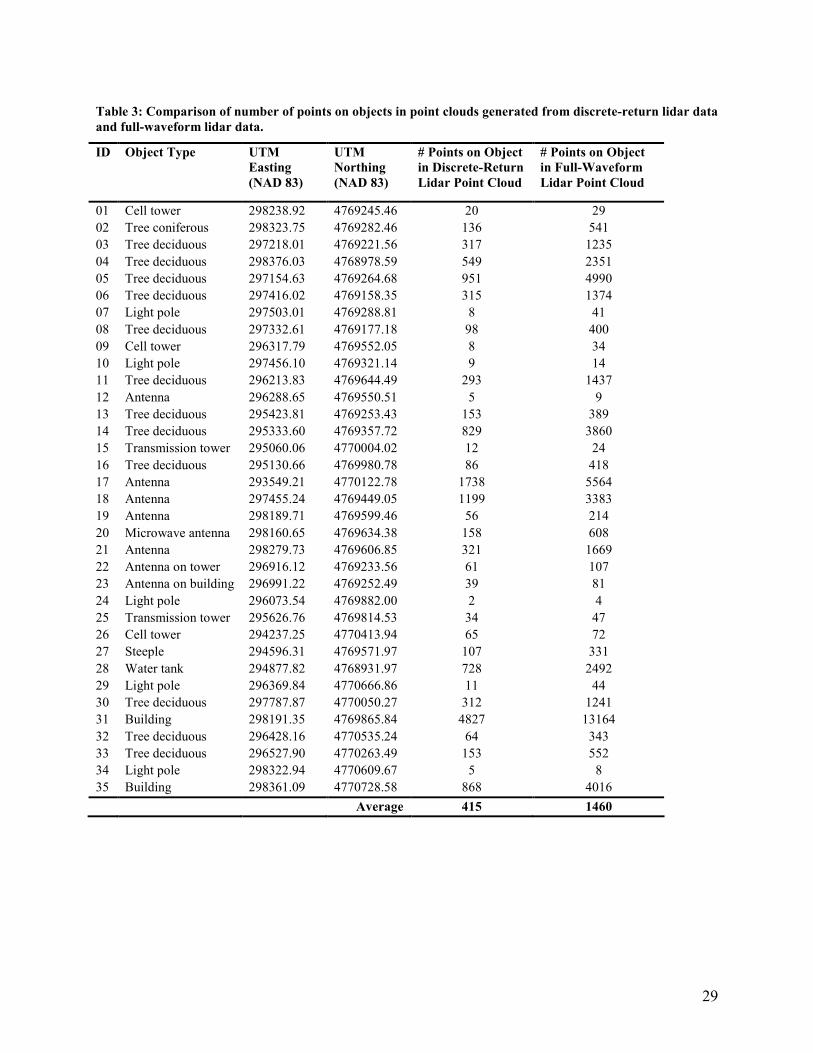
To investigate the achievable densification of point clouds for obstructions using the full-
waveform data, the point clouds output from Step 1 were compared against the point clouds
output from REALM using the discrete-return data. The first step in the analysis was to create
point cloud subsets around each of the field-surveyed objects in the southwest project area and to
use the “Measure Point Density” tool in TerraScan v5.005 (TerraSolid, Ltd.) to count the number
of points on each object. This semi-automated analysis was supplemented by manual analysis,
which entailed visually examining the output point clouds for each object in profile mode in
20
TerraScan to compare both the relative point densities and the relative amounts of noise. The
results of this analysis were quite promising: the use of the full-waveform data led to a 252%
increase in the average number of points on the objects, as shown in Table 3, with very slight
increase in the amount of noise in the point clouds on or near the objects, as seen in Fig. 6. This
figure shows photos (left column) and profile views of point cloud subsets for two different VOs,
a tree and TV broadcast tower, generated using the discrete-return lidar data (middle column)
and full-waveform data (right column). The gray values in the point cloud subsets represent
intensity and have been linearly stretched to span the available 8-bit (0-255) dynamic range. The
increase in point density on VOs that can be achieved using the full-waveform data is readily
apparent through comparison of the point cloud subsets in the middle and rightmost sections of
the figure. This increase in point density is especially important in detection of small, low-
reflectance objects, such as poles. For example, two laser points on an object may be too few to
enable detection or to reliably distinguish between object and noise, while four may be sufficient
(e.g. Object #24).
The next step was to investigate the ability to automatically eliminate false alarms and
correctly identify required objects in Steps 3 and 4 of our workflow. This was performed by
analyzing the input and output to Step 3 (OIS analysis) and comparing the final output from Step
4 (manual QA/QC and attribution) against the results obtained using the field-surveyed reference
data. The input to Step 3 consisted of 531 registered detections output from Step 2, including
both correct detections of real objects and false alarms (“false objects”). These detections were
analyzed against the OIS, depicted in Fig. 7, using the SML software. Software variables were
set to only output objects that penetrated, or came within 1.5 m of penetrating the OIS, resulting
in 529 objects being automatically eliminated and 2 being flagged as penetrating. The output

21
objects were then attributed using the DSS imagery in ArcGIS (Step 4). The final results were
compared with the output generated by running the reference data through NGS’ OIS analysis
software, and were found to match exactly: in both final data sets, Objects 17 and 18 were listed
as penetrating and attributed as antennas. No “false objects” needed to be analyzed and
eliminated in Step 4, as they were all automatically eliminated in Step 3 (OIS analysis).
The final analysis step was to compare the total time required to complete the obstruction
survey, as well as the required human time, with the corresponding times from NGS’ 2003 lidar
obstruction survey of Stafford Regional Airport (RMN) (described in Parrish et al. 2004). (This
comparison focused solely on the times required to survey obstructions and generate final
obstruction lists with object-type attributes; times required to complete other aspects of airport
surveys, such as profiling runways and geolocating navigational aids (FAA 1996; FAA 2008)
that were outside the scope of this study were not considered.) The results of the comparison
clearly demonstrated the efficiency of our workflow; the decrease in total (end-to-end)
obstruction survey time was approximately 46%, and the decrease in required human time was
38%.
Discussion and Conclusions
Following a decade of research by NGS and others into the capability to perform airport
obstruction surveys using lidar, we have developed and tested a new workflow with the goal of
making such surveys not only feasible, but also efficient and cost-effective. One key to the
workflow presented here is the use of the full-waveform data, which was shown to enable
generation of dense, detailed point clouds, which are well suited for this application. Equally
important is the ordering of steps in the workflow, in particular the placement of the VO

22
detection step before the OIS analysis and QA/QC. This sequence was shown to enable the
detection threshold to be set very conservatively, minimizing the probability of a missed
obstruction. Additionally, the amalgamation of steps requiring manual analysis minimizes the
amount of human time in the process, and the overall workflow has been designed to reduce the
total survey time. The 46% decrease in total (end-to-end) obstruction survey completion time
and 38% decrease in required human time, as compared with the most recent NGS lidar
obstruction survey, are quite encouraging.
Future work being planned by NGS includes conducting additional tests at two airports in
different parts of the United States with differing terrain and land cover/land use types, testing
and comparing different VO detection algorithms in Step 2 of the workflow described in this
paper, and continuing to refine the procedures for production use. It is anticipated that these
efforts, building upon the results presented here, will enable implementation of a wide-scale,
production lidar airport obstruction surveying program in the very near future.
Acknowledgements
The work described in this paper stems from the first author’s dissertation research at University
of Wisconsin (UW) Madison. We are indebted to the following UW supervisory committee
members for their invaluable contributions: Professors Frank Scarpace, Alan Vonderohe, Amos
Ron, and Chin Wu. Additionally, we are extremely grateful for the assistance of the many
Optech, Inc. and NGS colleagues who assisted in various aspects of this study.

23
References
Anderson, F., Tuell, G., and Parrish, C. (2002). “Application of LIDAR for airport mapping and
obstacle detection.” Proc., 3rd Int. LIDAR Workshop: Mapping Geo-Surficial Processes
Using Laser Altimetry (CD-ROM), Columbus, Ohio.
Federal Aviation Administration (FAA). (1996). FAA no. 405: Standards for aeronautical
surveys and related products, 4th Ed., US Department of Transportation, Washington, D.C.
FAA. (2007). “The third party survey system (TPSS) website users guide.”
<https://tpss.faa.gov/tpss/ > (Jul. 21, 2008).
FAA. (2008). Advisory Circular 150/5300-18B: General Guidance and Specifications for
Submission of Aeronautical Surveys to NGS: Field Data Collection and Geographic
Information System (GIS) Standards,
<http://www.faa.gov/airports_airtraffic/airports/resources/advisory_circulars/> (Jul. 21,
2008).
Figueiredo, M., and Nowak, R. (2001). “Wavelet-based image estimation: an empirical Bayes
approach using Jeffreys’ noninformative prior.” IEEE Transactions on Image Processing,
10(9), 1322-1331.
Figueiredo, M.A.T., and Nowak, R.D. (2003). “An EM algorithm for wavelet-based image
restoration.” IEEE Transactions on Image Processing, 12(8).
Filin, S. (2001). “Calibration of airborne and spaceborne laser altimeters using natural surfaces.”
PhD dissertation, Ohio State University, Columbus, Ohio.
Gross, H., Jutzi, B., and Thoennessen, U. (2007). “Segmentation of tree regions using data of a
full-waveform laser.” Int. Archives of Photogrammetry, Remote Sensing, and Spatial
Information Sciences, 36, 3/W49A, 57-62.
24
Gutierrez, R., Neuenschwander, A., and Crawford, M.M. (2005). “Development of laser
waveform digitization for airborne LIDAR topographic mapping instrumentation.” Proc.,
IEEE IGARSS, (2), 1154-1157.
Hofton, M.A., Minster, J.B. and Blair, J.B. (2000). “Decomposition of laser altimeter
waveforms.” IEEE Transactions of Geoscience and Remote Sensing, 38(4), 1989-1996.
Hug, C., Ullrich, A., and Grimm, A. (2004). “LITEMAPPER-5600 – a waveform digitizing lidar
terrain and vegetation mapping system.” Int. Archives of Photogrammetry and Remote
Sensing, Vol. 36, Part 8/W2, 24-29.
Jutzi, B., and Stilla, U. (2006). “Range determination with waveform recording laser systems
using a Wiener Filter.” ISPRS Journal of Photogrammetry and Remote Sensing, 61(2), 95-
107.
Kay, S.M. (1993). Fundamentals of Statistical Signal Processing: Estimation Theory (Vol. I).
Prentice Hall, Upper Saddle River, New Jersey.
National Geodetic Survey (NGS). (2004). “Light detection and ranging (LIDAR) requirements:
scope of work for airport surveying.” <www.ngs.noaa.gov/RSD/AirportSOW.pdf> (Jul.
21, 2008).
NGS. (2008). “Surface Model Library.” <ftp://ftp.ngs.noaa.gov/dist/ASP/SML/> (Jul. 21, 2008).
Nayegandhi, A., Brock, J.C., Wright, C.W., and O’Connell, M.J. (2006). “Evaluating a small
footprint, waveform-resolving lidar over coastal vegetation communities.” Photogramm.
Eng. Remote Sens., 72(12), 1407-1417.
Nordin, L. (2006). “Analysis of waveform data from airborne laser scanner systems.” MS thesis,
Luleå Univ. of Technology, Luleå, Sweden.

25
Nowak, R., and Figueiredo, M. (2001). "Fast wavelet-based image deconvolution using the EM
algorithm." Proc. 35th Asilomar Conference on Signals, Systems, and Computers,
Monterey, Calif.
Optech (2006). Airborne laser terrain mapper (ALTM) waveform digitzer (Doc. No.
0028443/Rev B). Optech Incorporated, Toronto, Ontario, Canada.
Parrish, C.E. (2003). “Analysis of airborne laser-scanning system configurations for detecting
airport obstructions.” MS thesis, Univ. of Florida, Gainesville, Fla.
Parrish, C.E., Woolard, J., Kearse, B., and Case, N. (2004). “Airborne lidar technology for
airspace obstruction mapping.” EOM, 13(4), 18-23.
Parrish, C.E., Tuell, G.H., Carter, W.E., and Shrestha, R.L. (2005). “Configuring an airborne
laser scanner for detecting airport obstructions.” Photogramm. Eng. Remote Sens., 71(1),
37-46.
Parrish, C.E. (2007a). “Vertical object extraction from full-waveform lidar data using a 3D
wavelet-based approach.” PhD dissertation, Univ. of Wisconsin- Madison, Madison, Wis.
Parrish, C.E. (2007b). “Exploiting full-waveform lidar data and multiresolution wavelet analysis
for vertical object detection and recognition.” Proc., IEEE IGARSS, Barcelona, Spain,
2499-2502.
Pates, J.R., Jr. (1950). “Airport obstruction plans.” Journal, Coast and Geodetic Survey, (3), 39-
44.
Persson, Å., Söderman, U., Töpel, J., and Ahlberg, S. (2005). “Visualization and analysis of full-
waveform airborne laser scanner data.” Proc. ISPRS WG III/3, V/3 Workshop: Laser
scanning 2005, Enschede, the Netherlands.
26
Reitberger, J., Krzystek, P. and Stilla, U. (2006). “Analysis of full waveform LIDAR data for
tree species classification.” Int. Archives of Photogrammetry, Remote Sensing, and Spatial
Information Sciences, 36(3), 228-233.
Smith, J.T., Jr. (1981). A history of flying and photography in the Photogrammetry Division of
the National Ocean Survey. US Department of Commerce, Washington, D.C., 99.
Stoker, J. (2004). “Voxels as a representation of multiple-return lidar data.” Proc., ASPRS
Annual Conference (CD-ROM), American Society for Photogrammetry and Remote
Sensing, Bethesda, Md.
Tuell, G. (1987). Technical Development Plan for the Modernization of the Airport Obstruction
Charting Program. NOAA Charting Research and Development Laboratory, Office of
Charting and Geodetic Services, Rockville, Md., 2-11.
Uddin, W., and Al-Turk, E. (2002). “Airport obstruction space management using airborne lidar
three-dimensional digital terrain mapping.” Proc., Federal Aviation Administration
Technology Transfer Conf. (CD-ROM).
Vaughn, C.R., Bufton, J.L., Krabill, W.B., and Rabine, D. (1996). “Georeferencing of airborne
laser altimeter measurements.” Int. J. Remote Sensing, 17(11), 2185-2200.
Vosselman, G., Gorte, B.G.H., Sithole, G. and Rabbani, T. (2004). “Recognising structure in
laser scanner point clouds.” Int. Archives of Photogrammetry and Remote Sensing, 36, part
8/W2, 33-38.
Wagner, W., Ullrich, A., Ducic, V., Melzer, T., and Studnicka, N. (2006). “Gaussian
decomposition and calibration of a novel small-footprint full-waveform digitising airborne
laser scanner.” ISPRS Journal of Photogrammetry and Remote Sensing, 60(2), 100 - 112.
27
Walter, M.D. (2005). “Deconvolution analysis of laser pulse profiles from 3-D LADAR temporal
returns.” MS thesis, Air Force Institute of Technology, Wright-Patterson Air Force Base,
Ohio.
Wang, C., Hu, Y., and Tao, V. (2004). “Identification and Risk Modeling of Airfield
Obstructions for Aviation Safety Management.” Proc., XXth ISPRS Conference, Istanbul,
Turkey, 13-18.
Woods, D., Folley, C., Kwan, Y.-T., and Houshmand, B. (2004). “Automatic extraction of
vertical obstruction information from interferometric SAR elevation data.” Proc., IEEE
International Geoscience and Remote Sensing Symposium (IGARSS), 6, 3938-3941.

28
Table 1: Mission parameters for Madison, WI, airborne lidar data acquisition.
Mission Parameter Value
Dates of data acquisition June 23-24, 2006
Aircraft Dynamic Aviation Beechcraft King Air
Flying speed over ground 70 m/s (135 kts)
Survey altitude 800 m (AGL)
Lidar system Optech ALTM 3100 w/ waveform digitizer
Pulse energy 80 - 90 µJ @ 70 kHz
Pulse width 11 ns (+/- 2 ns)
Laser rep rate 70 kHz
Beam divergence Narrow (0.3 mrad)
Laser wavelength 1064 nm
Scan angle +/- 17.3°
Scan rate 49.8 Hz
Swath width 500 m
Nominal horizontal point spacing 0.7m x 0.7m
Table 2: Mission parameters for Madison, WI, digital imagery acquisition.
Mission Parameter Value
Dates of data acquisition September 14-15, 2006
Aircraft NOAA Cessna Citation
Flying speed over ground 77 m/s (150 kts)
Survey altitude 1,370 m (AGL)
Camera Applanix DSS 322
Focal length 60 mm
Pixel size 9 µm CCD array dimensions 4092 x 5436 pixels (along x across)
Ground Sample Distance (GSD) 21 cm
Bands RGB
Endlap 60%
Sidelap 30%
Footprint 840 x 1120 m (along x across)
29
Table 3: Comparison of number of points on objects in point clouds generated from discrete-return lidar data
and full-waveform lidar data.
ID Object Type UTM
Easting
(NAD 83)
UTM
Northing
(NAD 83)
# Points on Object
in Discrete-Return
Lidar Point Cloud
# Points on Object
in Full-Waveform
Lidar Point Cloud
01 Cell tower 298238.92 4769245.46 20 29 02 Tree coniferous 298323.75 4769282.46 136 541 03 Tree deciduous 297218.01 4769221.56 317 1235 04 Tree deciduous 298376.03 4768978.59 549 2351 05 Tree deciduous 297154.63 4769264.68 951 4990 06 Tree deciduous 297416.02 4769158.35 315 1374 07 Light pole 297503.01 4769288.81 8 41 08 Tree deciduous 297332.61 4769177.18 98 400 09 Cell tower 296317.79 4769552.05 8 34 10 Light pole 297456.10 4769321.14 9 14 11 Tree deciduous 296213.83 4769644.49 293 1437 12 Antenna 296288.65 4769550.51 5 9 13 Tree deciduous 295423.81 4769253.43 153 389 14 Tree deciduous 295333.60 4769357.72 829 3860 15 Transmission tower 295060.06 4770004.02 12 24 16 Tree deciduous 295130.66 4769980.78 86 418 17 Antenna 293549.21 4770122.78 1738 5564 18 Antenna 297455.24 4769449.05 1199 3383 19 Antenna 298189.71 4769599.46 56 214 20 Microwave antenna 298160.65 4769634.38 158 608 21 Antenna 298279.73 4769606.85 321 1669 22 Antenna on tower 296916.12 4769233.56 61 107 23 Antenna on building 296991.22 4769252.49 39 81 24 Light pole 296073.54 4769882.00 2 4 25 Transmission tower 295626.76 4769814.53 34 47 26 Cell tower 294237.25 4770413.94 65 72 27 Steeple 294596.31 4769571.97 107 331 28 Water tank 294877.82 4768931.97 728 2492 29 Light pole 296369.84 4770666.86 11 44 30 Tree deciduous 297787.87 4770050.27 312 1241 31 Building 298191.35 4769865.84 4827 13164 32 Tree deciduous 296428.16 4770535.24 64 343 33 Tree deciduous 296527.90 4770263.49 153 552 34 Light pole 298322.94 4770609.67 5 8 35 Building 298361.09 4770728.58 868 4016
Average 415 1460
30
Fig. 1. Workflow diagram for lidar airport obstruction surveying using full-waveform data.
31
Fig. 2. Examples of digitized lidar waveforms.
Fig. 3: Illustration of an “ideal” lidar waveform consisting of a train of spikes in time (left) and a more
realistic representation of an actual observed waveform (right).

32
Fig. 4. Examples of two observed lidar waveforms (top, green), Wiener-filtered versions (middle, blue), and
output of EM deconvolution algorithm (bottom, red).
Fig. 5. Madison, Wisconsin project areas. The full-waveform lidar coverage is shown in orange and light
blue. The simulated ANA LPV approach for the southwest project site is shown in yellow.

33
Fig. 6. Comparison of point density for two different VOs, a tree (top) and tower (bottom), in point clouds
generated using the discrete-return lidar data (middle) and full-waveform lidar data (right). Photos of the
two objects are shown at left. The gray values in the point cloud subsets represent intensity, and have been
linearly stretched to take advantage of the available 8-bit dynamic range. The achievable increase in point
density using full-waveform data is clearly seen through this comparison.
Fig. 7. OIS analysis for simulated runway and ANA LPV approach in southwest Madison project area. The
red points indicate locations of field-surveyed reference objects.