implicit estimation of ecological model parameters

Bull Math Biol (2013) 75:223–257DOI 10.1007/s11538-012-9801-6

O R I G I NA L A RT I C L E

Implicit Estimation of Ecological Model Parameters

Brad Weir · Robert N. Miller · Yvette H. Spitz

Received: 3 June 2012 / Accepted: 27 November 2012 / Published online: 5 January 2013© Society for Mathematical Biology 2013

Abstract We introduce an implicit method for state and parameter estimation andapply it to a stochastic ecological model. The method uses an ensemble of parti-cles to approximate the distribution of model solutions and parameters conditionedon noisy observations of the state. For each particle, it first determines likely valuesbased on the observations, then samples around those values. This approach has astrong theoretical foundation, applies to nonlinear models and non-Gaussian distri-butions, and can estimate any number of model parameters, initial conditions, andmodel error covariances. The method is called implicit because it updates the par-ticles without forming a predictive distribution of forward model integrations. As apoint of comparison for different assimilation techniques, we consider examples inwhich one or more bifurcations separate the true parameter from its initial approxi-mation. The implicit estimator is asymptotically unbiased, has a root-mean-squarederror comparable to or less than the other methods, and is accurate even with smallensemble sizes.

Keywords Parameter estimation · Ecology · Particle filters · Implicit sampling

1 Introduction

The parameters of ecological models control the growth and mortality rates of indi-vidual species, their limitation due to crowding, and their interactions: consumption

B. Weir (�) · R.N. Miller · Y.H. SpitzCollege of Earth, Ocean, and Atmospheric Sciences, Oregon State University, Corvallis,OR 97331, USAe-mail: [email protected]

R.N. MillerINRIA Grenoble Rhône-Alpes, Laboratoire Jean Kuntzman, 38041 Grenoble, France

mailto:[email protected]

224 B. Weir et al.

of one species by another or competition for a common resource. The actual valuesof the parameters are usually unknown and impossible to determine from in situ mea-surements alone. Furthermore, many models combine species into functional groups,e.g., a marine biogeochemical model with state variables for nutrients, phytoplank-ton, zooplankton, and detritus. Since different species dominate the composition ofthese groups in different oceanic regions (Longhurst 1995), the model parametersvary from region to region. For some models, particularly those with just one phy-toplankton group, parameters appropriate in one region are unable to produce modelstates consistent with data collected in another (Friedrichs et al. 2007). One possibil-ity is that the model has a variety of possible dynamical behaviors (Newberger et al.2003), and the different parameters lie on opposite sides of a bifurcation. Thus, inorder to properly predict the state, the model must be calibrated by adjusting the pa-rameters based on the agreement of the model output with observations of a specificecosystem. In this paper, we develop an algorithm that uses the answers to variationalproblems to efficiently sample from the probability distribution of model solutionsand parameters conditioned on the observational data. We limit our references belowto the techniques that are the most similar to our own. For an overview of many more,see Robinson and Lermusiaux (2002) and Gregg (2008).

Variational methods find an extremum of a cost/objective function that representsthe compatibility of the model and observed data. The two most well known arethe maximum likelihood estimate (ML/MLE) and its Bayesian counterpart, the max-imum a posteriori (MAP) estimate. The MLE (Lehmann and Casella 1998) is theglobal maximum of the likelihood function, the probability density of the observa-tions viewed as a function of the parameters. Research prior to assimilation oftensuggests that, for certain parameters, some values are more likely than others. TheBayesian approach is to treat these parameters as random variables and the prior in-formation as their background probability distribution. The role of the data is thento supplement the background distribution by conditioning on the observed values.After assimilation, the probability density of the parameters is called the posterior.It is the product of the likelihood and background density, and its mode is the MAPestimate. From the point of view of optimization, the only difference between the MLand MAP estimates is the cost function that is maximized.

If the model is deterministic, the likelihood has an explicit form, yet its gra-dient is often difficult to compute directly. One approach is to use integrationsof the model and its adjoint to find the gradient. This is the basis of the four-dimensional variational (4D-Var) adjoint method (Talagrand and Courtier 1987;Courtier and Talagrand 1987) applied extensively in meteorology. Lawson et al.(1995, 1996) use the variational adjoint and a limited-memory, quasi-Newton opti-mization technique to compute the MLE of the parameters of two ecological modelsbased on synthetically generated twin data. Likewise, Spitz et al. (2001) assimilatein situ measurements at the Bermuda Atlantic Time-series Study (BATS) station withthe variational adjoint to help build a model for the ecosystem of the region and op-timize its parameters. This technique is used to further develop and calibrate marineecosystem models by Friedrichs (2002), Zhao et al. (2005), and a collection of otherauthors too numerous to cite in total. An alternative approach is to use a derivative-free optimization method such as simulated annealing. Matear (1995) applies simu-lated annealing to compute the MAP estimate of the parameters for three different

Implicit Estimation of Ecological Model Parameters 225

ecological models of increasing complexity based on observations at Ocean WeatherShip Station “P” in the subarctic Pacific. The same approach and data from BATSand Ocean Weather Ship Station “I” is used by Hurtt and Armstrong (1996, 1999)to develop a four-component ecological model and find the MLE of its parame-ters. In general, both the likelihood function and the posterior density have multiplelocal maxima, and the optimization method must search for the global maximum.Vallino (2000) compares the performance of 12 different global methods for deter-mining the MLE of the parameters of a biogeochemical model. He finds that the twobest are simulated annealing and the Levenberg–Marquardt trust-region method (seethe Appendix) with a randomized starting point.

Even if the exact parameters are known, we do not expect our models to be perfect.Computational approximations, variability in external forcing, and representation er-rors all add uncertainty to the model predictions, which we represent as noise. Fora stochastic model, the likelihood and posterior are functions of both the parametersand solutions of the model. In most cases, the ML and MAP estimates of the pa-rameters alone are impossible to compute directly—the functions that they maximizeare intractable integrals over the space of model solutions. Ionides et al. (2006) findthe MLE indirectly through repeated model simulations. Their technique replaces theconstant parameter with a random walk whose step size decreases with each itera-tion of the approximation. As the step size approaches zero, the iterates converge inprobability to the MLE. It is also possible to treat the random model solutions asmissing data. The ML or MAP estimate is then the result of a stochastic extensionof the expectation-maximization (EM) algorithm (Dempster et al. 1977) that replacesthe expectation step with a Monte Carlo estimate (McLachlan and Krishnan 2008,Sect. 6).

A single point estimate is often an unsatisfactory representation of the distributionof possible parameters, especially if the cost function has multiple extrema. We usea Monte Carlo method to draw samples from the target distribution (the posterior) ofthe model solutions and parameters. The ensemble of samples, also called particles,forms a discrete representation of the target, and estimates of its moments, marginals,and modes follow from the same computations on the ensemble. Designing effi-cient sampling methods is nontrivial if the model is nonlinear (Miller et al. 1999;van Leeuwen 2009) or the dimension of the state and/or parameters is large (Snyderet al. 2008). The main obstacle for methods that do not assume a parameterized formis the collapse of the ensemble onto just a few particles. We sample using an implicitapproach first developed by Chorin and Tu (2009) and generalized and improvedupon by Chorin et al. (2010) and Morzfeld et al. (2012). To minimize the chance ofcollapse, this technique focuses its samples around MAP estimates of the model so-lutions and parameters. Here, the methodology is extended to include multiplicativemodel noise and parameter estimation.

Our implicit sampling algorithm proceeds in three steps for each particle:optimize, sample, and weigh (OSW). The first step uses the observations to de-termine the extrema of the target in a given domain, the second samples an ap-proximation to the target around those values, and the last weighs the samplesto account for the difference between the sampled and target density. Since it fo-cuses on high probability regions, implicit sampling generally requires fewer par-ticles than other Monte Carlo methods to form a representation of the target with

226 B. Weir et al.

a given accuracy. It is applicable as a smoother, which assimilates all observationsat once, or as a filter, which assimilates the observations in sequence and discardsthem thereafter. In general, it is a technique for sampling any probability distribu-tion, and the OSW algorithm is one of many possible implementations. For deter-ministic models, this algorithm is similar to the incremental mixture importancesampling with optimization (IMIS-opt) method of Raftery and Bao (2010). An al-ternative implicit sampling algorithm, which is particularly effective if the targetdistribution is heavily skewed, solves a second optimization problem to find a trans-formation of an approximate distribution into the exact target (Chorin et al. 2010;Morzfeld et al. 2012).

For comparison, we consider two other Monte Carlo methods: the ensembleKalman filter (EnKF; Evensen 2009) and sampling/sequential importance resampling(SIR; Gordon et al. 1993). EnKF assumes a parametric form for all distributions: theyare Gaussians with the ensemble mean and covariance. Even if the model and ob-servation functions are nonlinear, this assumption is often close enough to the truthto produce reasonable estimates. SIR is the basis for a collection of nonparametrictechniques called particle filters (Doucet et al. 2001). Both methods first form a pre-dictive/forecast distribution by integrating the model forward to the next observationtime. They differ in how they update this distribution to account for the observations.EnKF moves the particles to the point that minimizes the sum of the squared distanceto the prediction and the squared distance to the observation. SIR weighs the particleswith the probability they produced the observations. It then resamples the particleswith replacement, a method also known as the bootstrap (Efron 1979, 2003), to pro-duce an ensemble of uniformly weighted particles. Doron et al. (2011) and Simonand Bertino (2012) assimilate data for a coupled biogeochemical-physical model byapplying a method based on EnKF. Their approach uses an anamorphosis functionthat maps the state and parameters to a space where their distribution more closelyresembles a Gaussian. In our comparisons, we use this transformation as well. The ac-curacy of EnKF estimates are at their worst if the model and/or observation functionsare strongly nonlinear. Kivman (2003) shows that for the Lorenz (1963) equationsand the same number of particles, SIR produces a more accurate representation ofthe posterior than EnKF. Losa et al. (2003) improve Kivman’s results by exchang-ing the resampling with replacement in SIR with a smoothed bootstrap. This helpsprevent the collapse of the ensemble onto a single parameter value by introducing asmall amount of noise. A different option is to use a Metropolis–Hastings (Metropo-lis et al. 1953) accept/reject move based on the ratio of the weights of a proposalparticle drawn from the ensemble and the previously accepted particle (Dowd 2006,2007, 2011; Wilkinson 2010). Since these variations work with any particle filter,including the implicit filter, we consider just one resampling method. Although dif-ferent methods can offer some improvement, Kitagawa (1996, App. A) demonstratesthat any benefit is likely dominated by the error in the ensemble representation of thetarget.

There are many other approaches that we do not consider for comparison.One is to use particle filters to design proposal distributions for Markov chainMonte Carlo (MCMC) methods (Gilks and Berzuini 2001; Marjoram et al. 2003;Andrieu et al. 2010). Golightly and Wilkinson (2011) use the particle marginal


Metropolis–Hastings method of Andrieu et al. (2010) to estimate the parameters ofthe Lotka–Volterra equations. Their method picks a proposal parameter, then runs aparticle filter for the state through the complete set of observations. Based on the like-lihood of the proposal parameter, the method either accepts it or rejects it in favor ofthe previous parameter. In some respects, the implicit smoother described below canbe considered as an attempt to construct efficient proposal distributions for such anMCMC method. The reward for the added effort of solving optimization problems isthe reduction of the probability of rejecting a proposal parameter. The implicit filterthen provides a means of continuing this construction sequentially once the number ofobservations exceeds the available storage capacity. Yet another strategy is to build anadaptive representation of the model error (Sapsis and Lermusiaux 2009, 2012) thatincludes the uncertainty in the parameters. After forming this representation, the stateestimate accounts for errors in the parameter values (Cossarini et al. 2009). Our goalis instead to find the parameter values that are likely to have lead to the observations.

The remainder of this paper is divided into 5 sections and an appendix. In thenext section, we define the data assimilation problem and introduce importance sam-pling. We present the implicit smoother in Sect. 3 and the implicit filter in Sect. 4.Both methods are applied to a stochastic model that is an extension of the Lotka–Volterra equations, and the statistics of their estimation errors are compared to thoseof EnKF and SIR in Sect. 5. We summarize our results and highlight other possi-ble topics for investigation in the concluding section. The Appendix describes ouroptimization method of choice and provides the model derivatives necessary for itsimplementation. Throughout the paper, the words “particle” and “sample” are usedinterchangeably, as are “Gaussian” and “normal”. When it improves the legibilityof the formulae, we drop the superscript particle index. All n-tuples denote columnvectors. For two integers l and k such that l ≤ k, we use the shorthand xl:k for thesequence {xl, . . . , xk}. Vector stochastic processes are printed in bold, uppercase let-ters and their realizations in bold, lowercase letters. If x is a random variable whoseprobability density function is p, we write either x ∼ p(x) or x ∼ p(x;μ,σ 2) to em-phasize the dependence of p on the parameters μ and σ .

2 Data Assimilation

We model the ecosystem as an Nx -dimensional stochastic process X that satisfies theIto equation

dX = f (X, θ) dt + G(X) dW. (1)

The variables are defined as follows: t denotes time; the drift f is a continuouslydifferentiable function of X and θ , a vector of parameters; the diffusion G is a non-singular Nx ×Nx matrix; and W is an Nx -dimensional vector of independent Wienerprocesses. Since few solutions of Eq. (1) have explicit forms, we compute a numericalapproximation Xm to X at a sequence of times {tm : m = 0,1, . . .}. The simplestapproach is the Euler–Maruyama method (Kloeden and Platen 1999) with a fixedtime step τ such that tm = mτ . Given the initial condition X0, the approximation form ≥ 1 follows from the iteration:

Xm = Xm−1 + τf (Xm−1, θ) + √τG(Xm−1)Em, (2)

228 B. Weir et al.

where the (dimensionless) model noise process {Em = (Wm − Wm−1)/√

τ } is a se-quence of scaled increments of the Wiener process. By definition, the incrementsare independent, identically distributed (iid) standard normal random variables. Wedenote their distribution as N (0, Ix), a multivariate Gaussian with mean zero andcovariance matrix Ix , the Nx × Nx identity.

At a subsequence {tm(n) : n = 1,2, . . .} of the model times, we observe a stochas-tic, Ny -dimensional function of the state

Yn = h(Xm(n)) + √RDn, (3)

where {Dn} is a sequence of iid standard normal random variables that are indepen-dent of the model noise process {Em}, and

√R is a given nonsingular, square matrix.

Although there is no observation at t0, we let m(0) = 0 to simplify notation. In prac-tice, the matrices G and

√R are unknown and must be estimated as well. Since we

consider examples with synthetically generated data, we assume that the matrices areknown. The generalization of implicit sampling to singular or nonsquare G and

√R

is straightforward (Morzfeld and Chorin 2012).Given a set of k observations y1:k and the background densities p(x0) and p(θ),

the posterior density

p(x0:m(k), θ | y1:k)

summarizes the entirety of our knowledge about the state and parameters. If its firsttwo moments are finite, the conditional expectation

E[θ | y1:k] =∫∫

θ p(x0:m(k), θ | y1:k) dx0:m(k) dθ (4)

is the uniformly unbiased estimator of θ with minimum root-mean-squared (RMS)error (Chorin and Hald 2009, Theorem 2.5). The same property is true for the condi-tional expectation of the path x0:m(k). If the posterior is multimodal, its mean, whilestill the best estimator on average, can be an uninformative representation of the dis-tribution as a whole. In this case, a better approach is to approximate its completeform with the samples—either as a histogram or scatter plot in low dimensions, or asa Gaussian mixture or collection of delta functions in high dimensions.

2.1 Importance Sampling

Direct evaluation of the conditional expectation (4) is rarely possible. If the observa-tions are continuous in time, rather than discrete, the posterior is the solution to theZakai equation (Zakai 1969). In special situations, the posterior for a discrete obser-vation process can also be expressed as the solution of a partial differential equation.Nevertheless, numerical solution of these equations is practical only if the dimen-sion of (x, θ) is around 4 or less. The last resort is to use a Monte Carlo methodto approximate the integral by sampling. The simplest and most efficient method isnot, remarkably, to always generate samples with the target density p (Ripley 1987).Rather, we approximate the integral (4) using importance sampling as follows (seeGeweke 1989, for a rigorous treatment). First, select an importance density q that is


easy to sample and is as close to the integrand as possible. Next, rewrite the condi-tional expectation as

E[θ | y1:k] =∫∫

θp(x0:m(k), θ | y1:k)q(x0:m(k), θ | y1:k)

q(x0:m(k), θ | y1:k) dx0:m(k) dθ.

For i = 1,2, . . . ,Np , draw a sample

(x(i)

0:m(k), θ(i)

) ∼ q(x0:m(k), θ | y1:k),

and give it the weight

w(i) = p(x(i)

0:m(k), θ(i)

∣∣y1:k)/

q(x(i)

0:m(k), θ(i)

∣∣y1:k).

The importance weights w(1), . . . ,w(Np) correct for the fact that the samples are fromthe importance density q, not the target p. If the importance density satisfies the ap-propriate regularity conditions, the approximation

θ =[ Np∑

i=1

θ(i)w(i)

]/[ Np∑i=1

w(i)

]

converges almost surely to the conditional expectation (4) as Np → ∞. We must di-vide by the sum of the weights since the target is only known up to a multiplicativeconstant, the reciprocal of the partition function. This can introduce bias since theexpectation of the ratio of two random variables is not the ratio of their expectations.The added bias is acceptable because its limit is zero as the number of samples ap-proaches infinity. Furthermore, even if the value of the partition function is known,dividing by the sum of the weights typically reduces the RMS error of the estimate.There is a central limit theorem for the weighted samples as well. It states that therate of convergence in probability is O(

√Np) and independent of the dimension of

the sample space. On the other hand, if C√

Np is the lowest-order term of the conver-gence rate, the constant C is problem dependent. When the variance of the weights islarge, C can be so small that an accurate approximation of the expectation (4) requiresan unrealistic number of particles. The sampling approaches below keep this variancesmall by building an importance density q for each particle that closely resembles thetrue density p.

3 An Implicit Smoother

We begin with the derivation of a cost function for the additive noise problem, pa-rameters with no constraints, and a Gaussian importance density. The derivation forthe multiplicative noise problem and parameters with constraints follows from thechange of variables described in Sect. 5. We use Bayes’ theorem, the model dis-cretization (2), observation function (3), and the fact that the noise processes Em andDn are independent to show that

230 B. Weir et al.

p(x0:m(k), θ | y1:k) ∝ p(x0:m(k), θ) · p(y1:k | x0:m(k), θ)

= p(x0) · p(θ) ·m(k)∏m=1

p(xm | xm−1, θ) ·k∏

n=1

p(yn | xm(n)). (5)

Since the model and observation errors are Gaussian random variables, the condi-tional densities are

p(xm | xm−1, θ) = 1

(√

2πτ)Nx |G| exp

(−1

2eTmem

), (6)

p(yn | xm(n)) = 1

(√

2π)Ny |√R| exp

(−1

2dT

n dn

), (7)

where | · | is the determinant, and the realizations of the (dimensionless) noise pro-cesses are

em = (√

τG)−1[xm − xm−1 − τf (xm−1, θ)],

dn = (√

R)−1[yn − h(xm(n))].

Substituting Eqs. (6) and (7) for the conditional densities into Eq. (5) results in therelationship

p(x0:m(k), θ | y1:k) ∝ p(x0) · exp(−J )

for the cost function J , defined such that

J = ln p(θ)−1 + 1

2

m(k)∑m=1

eTmem + 1

2

k∑n=1

dTn dn. (8)

We suppose the first term, and hence the cost function as a whole, is bounded below.We make no further assumptions about the cost function. In the following specialcase, our algorithm is equivalent to optimal sequential importance sampling (Doucetet al. 2000; Arulampalam et al. 2002): the observation function h is linear, the modelfunction f is a linear function of the parameter θ , and either (a) f is a linear functionof the state X, or (b) there are observations every time step, i.e., m(n) = n.

To assess the effectiveness of the parameter estimation, we produce two types ofsamples from the target: values of both the model solution and parameter and valuesof the model solution at a fixed parameter. For the OSW algorithm below, the onlydifference is the definition of the sampled variable ζ and fixed variable η. We denotethis distinction by writing J = J (ζ | η). To sample both the state and parameter,define

ζ = (x1:m(k), θ), and η = (x0,y1:k).

To sample just the state, define

ζ = x1:m(k), and η = (x0, θ,y1:k).


In both cases, we suppose the initial condition x0 has already been sampled from itsbackground density p(x0) and is held fixed at this value. Although we do not, it ispossible to treat the initial condition as a parameter. This is equivalent to including itin the definition of the sampled variable ζ , rather than the fixed variable η.

Algorithm 1 (Optimize, Sample, Weigh; OSW) Given a cost function J and fixedvariable η, this procedure produces a sample ζ with weight w from the probabilitydensity

p(ζ | η) ∝ exp[−J (ζ | η)

].

The algorithm has three steps:

1 Find the minimum ζ ∗ of the cost function.This is the MAP estimate of ζ given the data η. We use the trust-region methodoutlined in the Appendix to approximate ζ ∗.

2 Sample ζ from the multivariate Gaussian approximation of p(ζ | η) about ζ ∗.Let J ∗ = J (ζ ∗), and let H denote the Hessian of J at ζ ∗. To draw samples, firstform the quadratic approximation of the cost function

K(ζ) = J ∗ + 1

2

(ζ − ζ ∗)T

H(ζ − ζ ∗).

Since ζ ∗ is a local minimum, the Hessian is symmetric and positive semidefinite.Furthermore, it is positive definite if the model covariance R is nonsingular andp(θ) is a proper density. Both of theses properties are true for all of the exampleswe consider. Thus, a lower triangular Cholesky factor L of H exists such that

K(ζ) = J ∗ + 1

2

(ζ − ζ ∗)T

LLT(ζ − ζ ∗)

= J ∗ + 1

2

[LT

(ζ − ζ ∗)]T [

LT(ζ − ζ ∗)].

Finally, draw a sample ξ from a multivariate standard Gaussian with the samedimension as ζ and transform this into

ζ = ζ ∗ + L−T ξ.

3 Weigh the sample to account for the difference between the target and importancedensities.The importance weight is the ratio

w = p(ζ | η)/q(ζ |η)

∝ exp[−J (ζ )

]/|H |1/2 exp

[−1

2

(ζ − ζ ∗)T

H(ζ − ζ ∗)]

= ∣∣L−T∣∣ exp

(−J ∗) exp[K(ζ) − J (ζ )

].

232 B. Weir et al.

The factor exp[K(ζ) − J (ζ )] penalizes a particle if the quadratic approximationis far from the cost function. The factor |L−T | exp(−J ∗) gives greater weightsto particles that lead to sharper and smaller minima of the cost function. It canapproach ∞·0 if the dimension of ζ is large. For this reason, it is better to computeand store lnw than w.

To approximate the conditional expectation of the model state and parameters, wefirst generate an ensemble of iid initial positions

{x(i)

0 : i = 1, . . . ,Np

} ∼ p(x0).

We then apply Algorithm 1 to each particle to obtain an ensemble of importancesamples

{(x(i)

0:m(k), θ (i)

),w(i)

} ∼ p(x0:m(k), θ | y1:k).

Their weighted averages are the smoother estimates

x0:m(k) =[∑

i

w(i)x(i)0:m(k)

]/[∑i

w(i)

], (9a)

θ =[∑

i

w(i)θ (i)

]/[∑i

w(i)

]. (9b)

Since we apply Algorithm 1 to each particle individually, the importance density isthe pointed collection of Gaussians

q(x0:m(k), θ | y1:k) ∝∑

i

δ(x0 − x(i)

0

)q(x1:m(k), θ

∣∣x(i)0 ,y1:k

),

where δ is the Dirac delta function, and

q(x1:m(k), θ

∣∣ y1:k,x(i)0

) = N(x1:m(k), θ; ζ ∗(i),

[H(i)

]−1).

These distributions vary from particle to particle due to the dependence of the fixedvariable η on the initial position. Although we do not optimize over x0, Eq. (9a)estimates its actual value since samples closer to the truth have greater weights thanfarther samples. The application of our methodology to the estimation of the elementsof the model error G proceeds exactly as the estimation of θ . The only added effortis the computation of the derivatives of the realization of the model noise em withrespect to the elements of G.

4 An Implicit Filter

Suppose, after assimilating observations y1:l , we wish to assimilate k new observa-tions yl+1:l+k . One solution is to compute the smoother estimates (9a) and (9b) againfor the expanded set of observations y1:l+k . However, the time and storage require-ments of this computation grow without bound as l → ∞. Another solution, which


is possible because the target satisfies a recursion relation, is to assimilate the obser-vations in sequence. An application of Bayes’ theorem, the Markov property of thestate, and the conditional independence of the observations shows that

p(x0:m(l+k), θ | y1:l+k) ∝ p(x0:m(l+k), θ) · p(y1:l+k | x0:m(l+k), θ)

= p(x0:m(l), θ) ·m(l+k)∏

m=m(l)+1

p(xm | xm−1, θ)

· p(y1:l | x0:m(l)) ·l+k∏

n=l+1

p(yn | xm(n)).

Applying Bayes’ theorem once more,

p(x0:m(l+k), θ | y1:l+k) ∝ p(x0:m(l), θ | y1:l ) ·m(l+k)∏

m=m(l)+1

p(xm | xm−1, θ)

·l+k∏

n=l+1

p(yn | xm(n))

= p(x0:m(l), θ | y1:l ) · exp(−J ), (10)

where, by the definitions of the model noise (6) and observation noise (7), the costfunction for the filter is

J = 1

2

m(l+k)∑m=m(l)+1

eTmem + 1

2

l+k∑n=l+1

dTn dn. (11)

Since the recursion relation (10) holds for any l, we can apply it repeatedly, replacingl with l + k after each use. If k = 1, this approach is called a filter. We use thisterminology even if k = 1, although the name fixed-lag smoother is more appropriate.

The filter estimate proceeds by induction on the number l. During each assimila-tion, we sample just the new segment xm(l)+1:m(l+k) of the path, keeping the previoussegment x0:m(l) and parameter θ fixed. For the first step, we use the background dis-tributions to generate an ensemble of Np iid initial positions and parameters

{(x(i)

0 , θ(i)),w

(i)0 = 1/Np

} ∼ p(x0, θ).

Each step then begins with an ensemble of importance samples from the previoustarget

{(x(i)

0:m(l), θ(i)

),w

(i)l

} ∼ p(x0:m(l), θ | y1:l),

for an arbitrary l ≥ 0, where we use the convention that y1:0 = ∅. To assimilate thenew observations yl+1:l+k , we apply Algorithm 1 to each particle using the filter costfunction (11) with the sampled and fixed variables defined such that

ζ (i) = x(i)m(l)+1:m(l+k), and η(i) = (

x(i)m(l), θ

(i),yl+1:l+k

).

234 B. Weir et al.

The result is a collection of importance samples

{(x(i)

0:m(l+k), θ(i)

),w

(i)l+k = w(i) · w(i)

l

} ∼ p(x0:m(l+k), θ | y1:l+k),

where w(i) is the weight returned by Algorithm 1. These samples serve as the startingpoint for the next step of the induction. In analogy with the smoother estimates (9a)and (9b), the filter estimates are the weighted averages

xm(l)+1:m(l+k) =[∑

i

w(i)l+kx(i)

m(l+1):m(l+k)

]/[∑i

w(i)l+k

], (12a)

θ =[∑

i

w(i)l+kθ

(i)

]/[∑i

w(i)l+k

]. (12b)

Most importantly, after sampling the new segment of the path, we can discard theobservations and the previous segment. The computation time and storage of eachassimilation are thus independent of l.

Since each application of the recursion relation (10) multiplies the previous par-ticle weight with the weight from the new assimilation, after many iterations, all buta few particles can have negligible weights. This significantly degrades the qualityof the filter estimates (12a) and (12b). For state estimation, the usual solution is toresample with replacement (Efron 1979, 2003), which transforms the weighted sam-ples into a uniformly weighted ensemble drawn from the same distribution. This isinsufficient for parameter estimation—resampling from a static set of parameters willeventually eliminate all but one, leaving no way to improve the estimate. To preventthis, Liu and West (2001) propose the inclusion of a kernel density estimate for theparameters such that the representation of the previous target is

p(x0:m(l), θ | y1:l ) ≈Np∑i=1

w(i)l δ

(x0:m(l) − x(i)

0:m(l)

)K(i)(θ), (13)

where w(i)l = w

(i)l /[∑w

(i)l ]. As the kernel densities, we pick Gaussians

K(i) = N(μ + c

(θ(i) − μ

), (ch)2Σ

),

where μ and Σ are the sample mean and covariance of θ , h is the kernel bandwidth,and c is a constant that adjusts the diffusion of the kernel representation. We use theoptimal bandwidth h for Gaussian targets (Silverman 1986, Sect. 4.3) and define c

such that Σ remains the covariance of θ . If Nθ is the number of estimated parameters,then

h = [4/(Nθ + 2)

]1/(Nθ+4)N

−1/(Nθ+4)p ,

c = 1/√

1 + h2.

In the limit Np → ∞, the kernel densities K(i) approach delta functions at θ(i) be-cause h → 0 and c → 1. While our choices for h and c are usually acceptable, they


are suboptimal for non-Gaussian targets. Silverman (1986) discusses this issue indetail and suggests possible improvements, which we do not consider here. In partic-ular, the choice for c is intended to prevent additional diffusion of the particles fromthe kernel density representation. For small numbers of particles, c is often too smallto prevent the ensemble from collapsing onto a single parameter value.

After each assimilation, we compute the effective number of particles (Doucetet al. 2000)

Neff = 1/

[∑i

(w

(i)l

)2].

If this number drops below Np/4, we use the following algorithm to resample fromthe kernel density estimate (13) of the target.

Algorithm 2 (Smoothed bootstrap) This procedure takes an ensemble of Np impor-tance samples {(

x(i)0:m(l), θ

(i)),w

(i)l

} ∼ p(x0:m(l), θ | y1:l),

and transforms it into an ensemble of samples from the same distribution with uni-form weights, {(

x(i)0:m(l), θ

(i)), w

(i)l = 1/Np

} ∼ p(x0:m(l), θ | y1:l).

We apply each of the steps below to each particle before moving on to the next step.

1 Compute the normalized weights w(i)l = w

(i)l /[∑w

(i)l ].

2 Find the resampling indices ki as follows.Generate a random number ui ∈ (0,1]. If ui ≤ w

(1)l , let ki = 1. Otherwise, find ki

such thatki−1∑j=1

w(j)l < ui ≤

ki∑j=1

w(j)l .

3 Resample the states and parameters such that

x(i)0:m(l) = x(ki )

0:m(l),

θ (i) ∼ N(θ;μ + c

(θ(ki ) − μ

), (ch)2Σ

),

and set w(i)l = 1/Np .

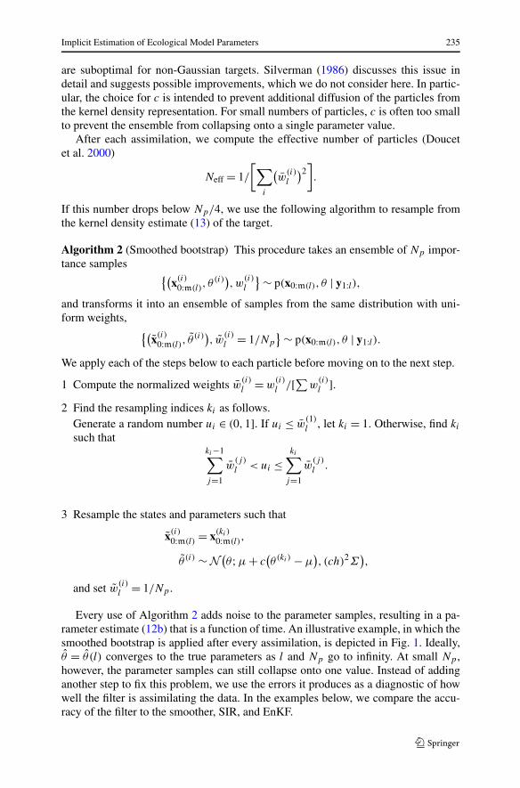
Every use of Algorithm 2 adds noise to the parameter samples, resulting in a pa-rameter estimate (12b) that is a function of time. An illustrative example, in which thesmoothed bootstrap is applied after every assimilation, is depicted in Fig. 1. Ideally,θ = θ (l) converges to the true parameters as l and Np go to infinity. At small Np ,however, the parameter samples can still collapse onto one value. Instead of addinganother step to fix this problem, we use the errors it produces as a diagnostic of howwell the filter is assimilating the data. In the examples below, we compare the accu-racy of the filter to the smoother, SIR, and EnKF.

236 B. Weir et al.

Fig. 1 Schematic for the filter estimates (12a) and (12b). The vertical bars represent a standard devi-ation of the kernel density K(i). Here, we assimilate one observation at a time and apply Algorithm 2immediately afterward

5 The Lotka–Volterra Equations

The Lotka–Volterra equations (Brauer and Castillo-Chavez 2012) describe the dy-namical evolution of the concentrations of a predator Q and its prey P . We use a mod-ified, Holling-type interaction term (Holling 1959) originally proposed by Michaelisand Menten (1913) as a model for enzymatic reactions (see Johnson and Goody 2011,for an English translation and analysis). The Michaelis–Menten term typically ap-pears in marine ecology models as a parameterization of the limitation of uptake ofa nutrient P by phytoplankton Q (Fasham et al. 1990). We consider it here becausethe model equations have a richer dynamical structure than they do with the originalinteraction term. In deterministic form, the equations are

dP

dt= (a1 + a2P)P + a3

PQ

1 + a7P,

dQ

dt= (a4 + a5Q)Q + a6

PQ

1 + a7P.

(14)

A complete description of the state and model parameters is in Table 1. Since P andQ are concentrations, they are always nonnegative. In order to preserve the predator-prey relationship between P and Q, the parameters are also constrained to take onlyone sign. We fix a5 = 0 since the death rate of the predator limits its concentration.Henceforth, we let the model state and parameter variables denote both their dimen-


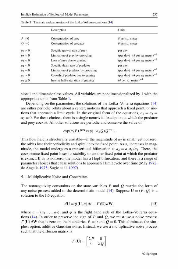
Table 1 The state and parameters of the Lotka-Volterra equations (14)

Description Units

P ≥ 0 Concentration of prey # per sq. meter

Q ≥ 0 Concentration of predator # per sq. meter

a1 > 0 Specific growth rate of prey per day

a2 < 0 Limitation of prey by crowding (per day) · (# per sq. meter)−1

a3 < 0 Loss of prey due to grazing (per day) · (# per sq. meter)−1

a4 < 0 Specific death rate of predator per day

a5 = 0 Limitation of predator by crowding (per day) · (# per sq. meter)−1

a6 > 0 Growth of predator due to grazing (per day) · (# per sq. meter)−1

a7 ≥ 0 Inverse half-saturation of grazing (# per sq. meter)−1

sional and dimensionless values. All variables are nondimensionalized by 1 with theappropriate units from Table 1.

Depending on the parameters, the solutions of the Lotka–Volterra equations (14)are either periodic orbits about a center, motions that approach a fixed point, or mo-tions that approach a limit cycle. In the original form of the equations, a2 = a5 =a7 = 0. For these choices, there is a single nontrivial fixed point at which the predatorand prey coexist. All other solutions are periodic and conserve the value of

exp(a6P)P a4 exp(−a3Q)Q−a1 .

This flow field is structurally unstable—if the magnitude of a2 is small, yet nonzero,the orbits lose their periodicity and spiral into the fixed point. As a2 increases in mag-nitude, the model undergoes a transcritical bifurcation at a2 = a1a6/a4. There, thecoexistence fixed point loses its stability to another fixed point at which the predatoris extinct. If a7 is nonzero, the model has a Hopf bifurcation, and there is a range ofparameter choices that cause solutions to approach a limit cycle over time (May 1972;de Angelis 1975; Sugie et al. 1997).

5.1 Multiplicative Noise and Constraints

The nonnegativity constraints on the state variables P and Q restrict the form ofany noise process added to the deterministic model (14). Suppose U = (P,Q) is asolution to the Ito equation

dU = φ(U, a) dt + Γ (U) dW, (15)

where a = (a1, . . . , a7), and φ is the right hand side of the Lotka–Volterra equa-tions (14). In order to preserve the sign of P and Q, we must use a noise processΓ (U) dW that is zero on the boundaries P = 0 and Q = 0. This eliminates the sim-plest option, additive Gaussian noise. Instead, we use a multiplicative noise processsuch that the diffusion matrix is

Γ (U) =[

λP 00 λQ

]

238 B. Weir et al.

for a given parameter λ such that λ−2 is in units of days. There are many otherpossible choices for Γ . Øksendal (2003, Theorem 5.2.1) gives sufficient, yet notnecessary, conditions such that the initial value problem for Eq. (15) has unique,bounded solutions for all time. If Γ is a diagonal matrix with entries λP α and λQα ,the conditions are only satisfied when α = 1. If α > 1, the diffusion fails to satisfythe linear growth condition, while if α < 1, it fails the Lipschitz continuity conditionat the origin.

We use a change of variables to reduce the multiplicative noise problem with con-straints on the parameters to an additive noise problem with no constraints. Let theunconstrained model state and parameter be

X = (lnP, lnQ),

θ = (ln |a1|, . . . , ln |a4|, a5, ln |a6|, a7).

Here, we do not transform a5 and a7 since they are kept constant in the examples tofollow. The transformations are equivalent to the anamorphosis functions of Doronet al. (2011) and Simon and Bertino (2012), and we use them for all techniques con-sidered. Applying Ito’s lemma to Eq. (15) for the change of variables X = X(U), werecover Eq. (1), where the drift and diffusion are

f (X, θ) =[e−X1 0

0 e−X2

]φ(X, θ) − 1

2

[λ2

λ2

]

=[a1 + a2P + a3Q/(1 + a7P) − λ2/2a4 + a5Q + a6P/(1 + a7P) − λ2/2

]and G =

[λ 00 λ

].

The observation function (3) changes form as well. In particular, a linear observa-tion of X is an observation of the logarithm of U, and the exponential of such anobservation is a linear observation of U with multiplicative noise, i.e., if h(X) = X,then

exp(Yn) = Un exp(√

RDn). (16)

Since our goal is unbiased estimates of the original state U and parameter a, we com-pute their weighted averages instead of those of X and θ in the implicit estimates (9a),(9b), (12a) and (12b).

The theory of bifurcations of a stochastic process is still an active area of research(Arnold 1998, Chap. 9). Roughly, a change in the stability of an invariant set of thedeterministic model (14) corresponds to a qualitative change in the invariant measureof the stochastic model (15). To construct an approximation of the invariant measure,we divide state space into bins and count the number of times a stochastic solutionis in each bin (following a sufficiently long equilibration time). If the noise is smallto moderate, the invariant measure is usually concentrated around a stable invariantset of the deterministic model, and the stochastic bifurcation occurs near the sameparameter values where the invariant set exchanges stability with another. In the ex-amples, we use a value of λ such that this property holds. This is for illustrativepurposes only, and we do not expect it to affect the applicability of the algorithms ingeneral.


5.2 Twin Experiments

To test the effectiveness of the parameter estimation, we consider two scenarios inwhich the initial approximation of a and its true value are separated by one or morebifurcations. The true parameter value is used in the stochastic model (15) to generatesynthetic observations of a reference solution. We then assimilate these observationsand compare the errors of the implicit estimates, SIR, and EnKF.

In every example, we make the following choices: λ2 = 0.04; the backgrounddistribution on the initial condition is a delta function at (P0,Q0) = (1,1); the back-ground on the parameters is a Gaussian such that

p(θ) = N(θ;μ,σ 2),

where μ is our initial approximation of θ , and σ is large enough that the effect of thebackground on the parameter estimates is minimal, a property we verify a posteriori.Since, by Bayes’ theorem,

p(θ | y1:k) ∝ p(θ) · p(y1:k | θ),

picking such a σ is possible if only if the observations depend on θ . If they do not, itis impossible to estimate θ based solely on y1:k , a scenario we do not consider.

Example 1 (Unobserved component, single parameter) Here, we estimate just a2,a parameter that controls the evolution of the prey P , while observing only the preda-tor Q. The time step τ is 10−3 days, and every two time steps we observe X2 = lnQ

a total of 1500 times with an error variance of R = 10−2. For our initial approxima-tion, we assume a2 = −4. As the background on θ2 = ln |a2| we pick the Gaussiandensity

p(θ2) = N (θ2; ln |−4|,1/2), (17)

which is centered around the initial approximation. The remainder of the parametersare held constant at their true values listed in Table 2. We return to the other values inTable 2 throughout the discussion of this example.

Between the initial approximation of a2 and its true value (see Table 2) is a tran-scritical bifurcation at a2 = −8/3. If a2 < −8/3, the population of the prey is insuf-ficient to support the predator, which goes extinct. Over time, all solutions approachthe stable fixed point

(P,Q) = (−a1/a2,0)

= (−4/a2,0).

If a2 > −8/3, the predator and prey coexist at nonzero concentrations. The extinctionfixed point is unstable, and there is a stable fixed point at

(P,Q) = (−a4/a6, (a2a4 − a1a6)/a3a6)

= (3/2,1 + 3a2/8).

240 B. Weir et al.

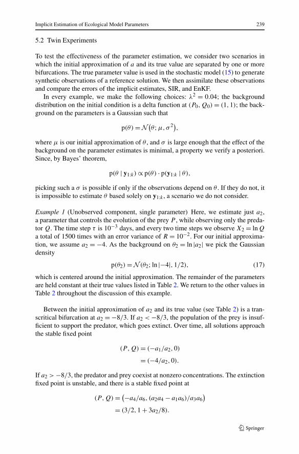
Table 2 Initial approximation, smoother estimate (9b), filter estimate (12b), standard deviations, and thetrue values of the parameter a for Example 1

Np a1 a2 a3 a4 a5 a6 a7

Initial 4 −4 −4 −6 0 4 0

Smoother 24 4 −2.1079 −4 −6 0 4 0

240 4 −2.1040 −4 −6 0 4 0

2400 4 −2.0995 −4 −6 0 4 0

24k 4 −2.0999 −4 −6 0 4 0

Std. dev. 240 0.0988

Filter 24 4 −2.0968 −4 −6 0 4 0

240 4 −2.1701 −4 −6 0 4 0

2400 4 −2.2007 −4 −6 0 4 0

24k 4 −2.1120 −4 −6 0 4 0

Std. dev. 240 0.0972

True 4 −2 −4 −6 0 4 0

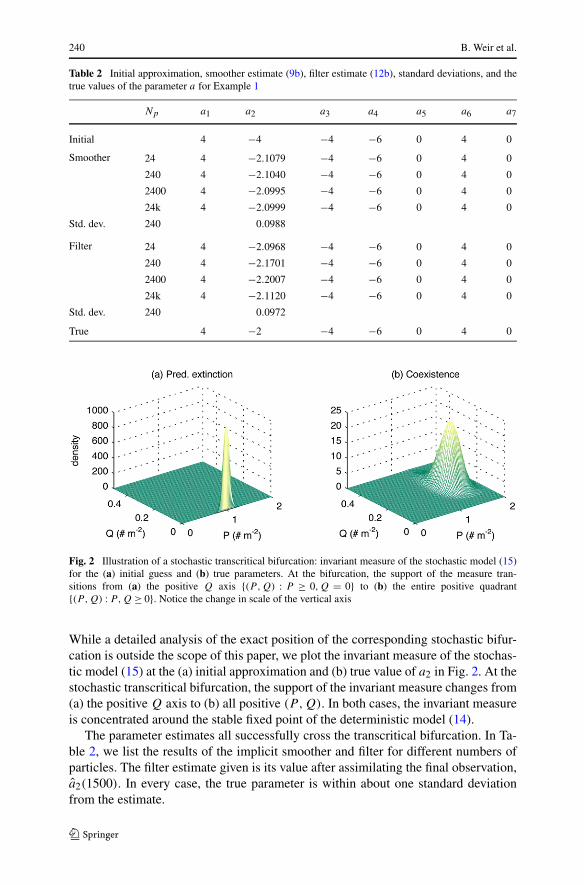
Fig. 2 Illustration of a stochastic transcritical bifurcation: invariant measure of the stochastic model (15)for the (a) initial guess and (b) true parameters. At the bifurcation, the support of the measure tran-sitions from (a) the positive Q axis {(P,Q) : P ≥ 0,Q = 0} to (b) the entire positive quadrant{(P,Q) : P,Q ≥ 0}. Notice the change in scale of the vertical axis

While a detailed analysis of the exact position of the corresponding stochastic bifur-cation is outside the scope of this paper, we plot the invariant measure of the stochas-tic model (15) at the (a) initial approximation and (b) true value of a2 in Fig. 2. At thestochastic transcritical bifurcation, the support of the invariant measure changes from(a) the positive Q axis to (b) all positive (P,Q). In both cases, the invariant measureis concentrated around the stable fixed point of the deterministic model (14).

The parameter estimates all successfully cross the transcritical bifurcation. In Ta-ble 2, we list the results of the implicit smoother and filter for different numbers ofparticles. The filter estimate given is its value after assimilating the final observation,a2(1500). In every case, the true parameter is within about one standard deviationfrom the estimate.


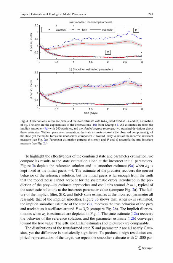
Fig. 3 Observations, reference path, and the state estimate with (a) a2 held fixed at −4 and (b) estimationof a2. The dots are the exponentials of the observations (16) from Example 1. All estimates are from theimplicit smoother (9a) with 240 particles, and the shaded regions represent two standard deviations aboutthese estimates. Without parameter estimation, the state estimate recovers the observed component Q ofthe state, yet the model forces the unobserved component P toward likely values of the incorrect invariantmeasure (see Fig. 2a). Parameter estimation corrects this error, and P and Q resemble the true invariantmeasure (see Fig. 2b)

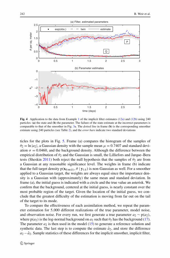
To highlight the effectiveness of the combined state and parameter estimation, wecompare its results to the state estimation alone at the incorrect initial parameters.Figure 3a depicts the reference solution and its smoother estimate (9a) when a2 iskept fixed at the initial guess −4. The estimate of the predator recovers the correctbehavior of the reference solution, but the initial guess is far enough from the truththat the model noise cannot account for the systematic errors introduced in the pre-diction of the prey—its estimate approaches and oscillates around P = 1, typical ofthe stochastic solutions at the incorrect parameter value (compare Fig. 2a). The fail-ure of the implicit filter, SIR, and EnKF state estimates at the incorrect parameter allresemble that of the implicit smoother. Figure 3b shows that, when a2 is estimated,the implicit smoother estimate of the state (9a) recovers the true behavior of the preyand tracks it as it oscillates around P = 3/2 (compare Fig. 2b). The implicit filter es-timates when a2 is estimated are depicted in Fig. 4. The state estimate (12a) recoversthe behavior of the reference solution, and the parameter estimate (12b) convergestoward the true value. The SIR and EnKF estimates (not pictured) are comparable.

The distributions of the transformed state X and parameter θ are all nearly Gaus-sian, yet the difference is statistically significant. To produce a high-resolution em-pirical representation of the target, we repeat the smoother estimate with 24,000 par-

242 B. Weir et al.

Fig. 4 Application to the data from Example 1 of the implicit filter estimates (12a) and (12b) using 240particles: (a) the state and (b) the parameter. The failure of the state estimate at the incorrect parameters iscomparable to that of the smoother in Fig. 3a. The dotted line in frame (b) is the corresponding smootherestimate using 240 particles (see Table 2), and the error bars indicate two standard deviations

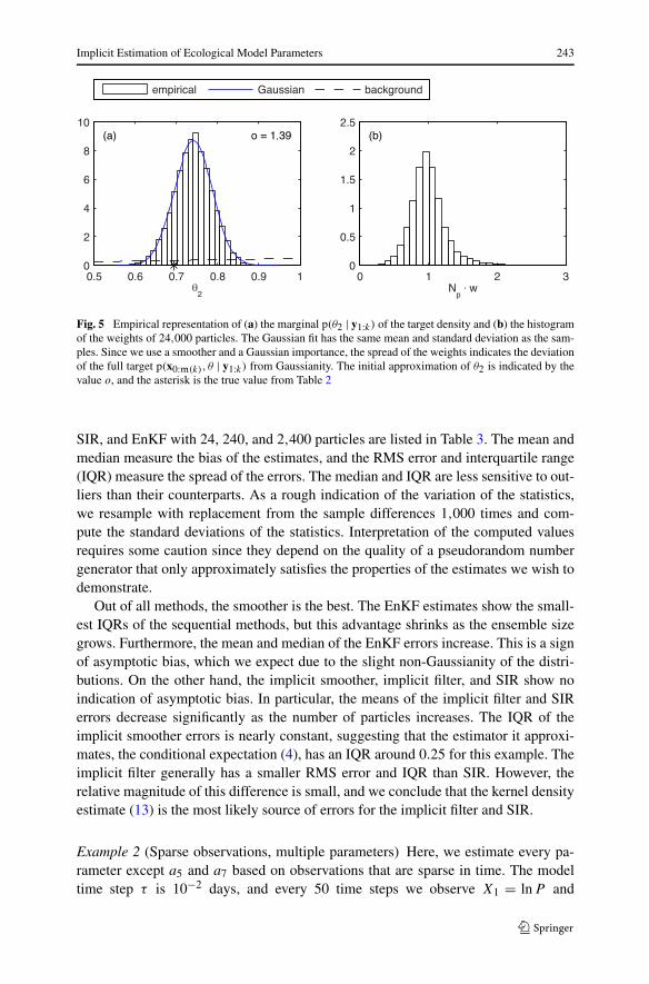
ticles for the plots in Fig. 5. Frame (a) compares the histogram of the samples ofθ2 = ln |a2|, a Gaussian density with the sample mean μ = 0.7407 and standard devi-ation σ = 0.0460, and the background density. Although the difference between theempirical distribution of θ2 and the Gaussian is small, the Lilliefors and Jarque–Beratests (Sheskin 2011) both reject the null hypothesis that the samples of θ2 are froma Gaussian at any reasonable significance level. The weights in frame (b) indicatethat the full target density p(x0:m(k), θ | y1:k) is non-Gaussian as well. For a smootherapplied to a Gaussian target, the weights are always equal since the importance den-sity is a Gaussian with (approximately) the same mean and standard deviation. Inframe (a), the initial guess is indicated with a circle and the true value an asterisk. Weconfirm that the background, centered at the initial guess, is nearly constant over themost probable region of the target. Given the location of the initial guess, we con-clude that the greatest difficulty of the estimation is moving from far out on the tailof the target to its mode.

To compare the effectiveness of each assimilation method, we repeat the param-eter estimation for 5,000 different realizations of the true parameter, model noise,and observation noise. For every run, we first generate a true parameter a2 ∼ p(a2),where p(a2) is the log-normal background on a2 such that θ2 has the background (17).The parameter a2 is then used in the model (15) to generate a reference solution andsynthetic data. The last step is to compute the estimate a2, and store the differencea2 − a2. Sample statistics of these differences for the implicit smoother, implicit filter,


Fig. 5 Empirical representation of (a) the marginal p(θ2 | y1:k) of the target density and (b) the histogramof the weights of 24,000 particles. The Gaussian fit has the same mean and standard deviation as the sam-ples. Since we use a smoother and a Gaussian importance, the spread of the weights indicates the deviationof the full target p(x0:m(k), θ | y1:k) from Gaussianity. The initial approximation of θ2 is indicated by thevalue o, and the asterisk is the true value from Table 2

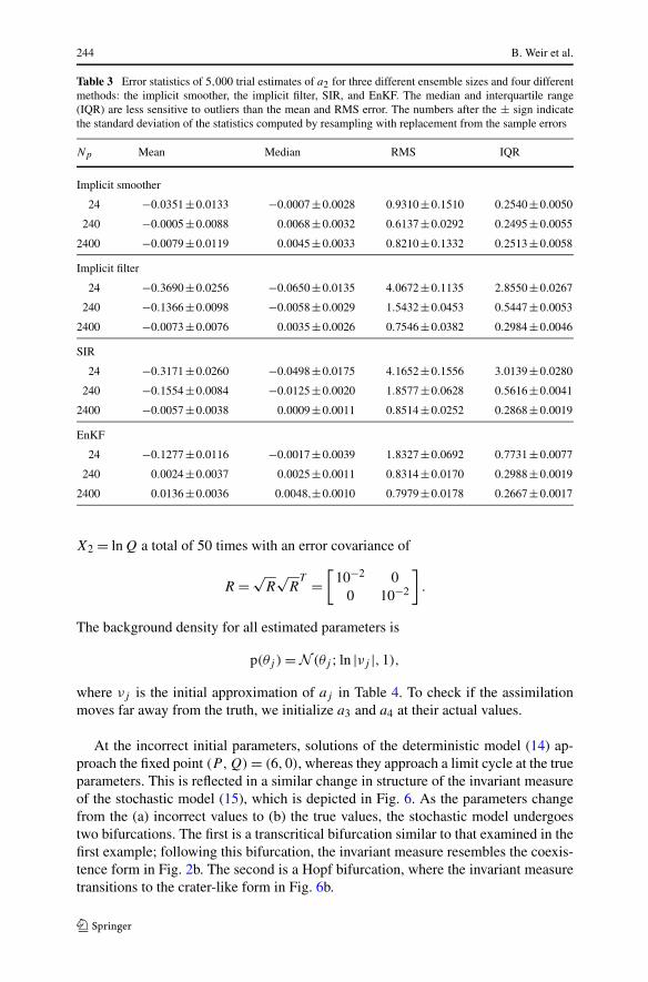
SIR, and EnKF with 24, 240, and 2,400 particles are listed in Table 3. The mean andmedian measure the bias of the estimates, and the RMS error and interquartile range(IQR) measure the spread of the errors. The median and IQR are less sensitive to out-liers than their counterparts. As a rough indication of the variation of the statistics,we resample with replacement from the sample differences 1,000 times and com-pute the standard deviations of the statistics. Interpretation of the computed valuesrequires some caution since they depend on the quality of a pseudorandom numbergenerator that only approximately satisfies the properties of the estimates we wish todemonstrate.

Out of all methods, the smoother is the best. The EnKF estimates show the small-est IQRs of the sequential methods, but this advantage shrinks as the ensemble sizegrows. Furthermore, the mean and median of the EnKF errors increase. This is a signof asymptotic bias, which we expect due to the slight non-Gaussianity of the distri-butions. On the other hand, the implicit smoother, implicit filter, and SIR show noindication of asymptotic bias. In particular, the means of the implicit filter and SIRerrors decrease significantly as the number of particles increases. The IQR of theimplicit smoother errors is nearly constant, suggesting that the estimator it approxi-mates, the conditional expectation (4), has an IQR around 0.25 for this example. Theimplicit filter generally has a smaller RMS error and IQR than SIR. However, therelative magnitude of this difference is small, and we conclude that the kernel densityestimate (13) is the most likely source of errors for the implicit filter and SIR.

Example 2 (Sparse observations, multiple parameters) Here, we estimate every pa-rameter except a5 and a7 based on observations that are sparse in time. The modeltime step τ is 10−2 days, and every 50 time steps we observe X1 = lnP and

244 B. Weir et al.

Table 3 Error statistics of 5,000 trial estimates of a2 for three different ensemble sizes and four differentmethods: the implicit smoother, the implicit filter, SIR, and EnKF. The median and interquartile range(IQR) are less sensitive to outliers than the mean and RMS error. The numbers after the ± sign indicatethe standard deviation of the statistics computed by resampling with replacement from the sample errors

Np Mean Median RMS IQR

Implicit smoother

24 −0.0351±0.0133 −0.0007±0.0028 0.9310±0.1510 0.2540±0.0050

240 −0.0005±0.0088 0.0068±0.0032 0.6137±0.0292 0.2495±0.0055

2400 −0.0079±0.0119 0.0045±0.0033 0.8210±0.1332 0.2513±0.0058

Implicit filter

24 −0.3690±0.0256 −0.0650±0.0135 4.0672±0.1135 2.8550±0.0267

240 −0.1366±0.0098 −0.0058±0.0029 1.5432±0.0453 0.5447±0.0053

2400 −0.0073±0.0076 0.0035±0.0026 0.7546±0.0382 0.2984±0.0046

SIR

24 −0.3171±0.0260 −0.0498±0.0175 4.1652±0.1556 3.0139±0.0280

240 −0.1554±0.0084 −0.0125±0.0020 1.8577±0.0628 0.5616±0.0041

2400 −0.0057±0.0038 0.0009±0.0011 0.8514±0.0252 0.2868±0.0019

EnKF

24 −0.1277±0.0116 −0.0017±0.0039 1.8327±0.0692 0.7731±0.0077

240 0.0024±0.0037 0.0025±0.0011 0.8314±0.0170 0.2988±0.0019

2400 0.0136±0.0036 0.0048,±0.0010 0.7979±0.0178 0.2667±0.0017

X2 = lnQ a total of 50 times with an error covariance of

R = √R

√R

T =[

10−2 00 10−2

].

The background density for all estimated parameters is

p(θj ) = N (θj ; ln |νj |,1),

where νj is the initial approximation of aj in Table 4. To check if the assimilationmoves far away from the truth, we initialize a3 and a4 at their actual values.

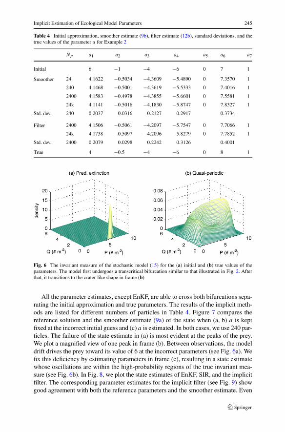
At the incorrect initial parameters, solutions of the deterministic model (14) ap-proach the fixed point (P,Q) = (6,0), whereas they approach a limit cycle at the trueparameters. This is reflected in a similar change in structure of the invariant measureof the stochastic model (15), which is depicted in Fig. 6. As the parameters changefrom the (a) incorrect values to (b) the true values, the stochastic model undergoestwo bifurcations. The first is a transcritical bifurcation similar to that examined in thefirst example; following this bifurcation, the invariant measure resembles the coexis-tence form in Fig. 2b. The second is a Hopf bifurcation, where the invariant measuretransitions to the crater-like form in Fig. 6b.


Table 4 Initial approximation, smoother estimate (9b), filter estimate (12b), standard deviations, and thetrue values of the parameter a for Example 2

Np a1 a2 a3 a4 a5 a6 a7

Initial 6 −1 −4 −6 0 7 1

Smoother 24 4.1622 −0.5034 −4.3609 −5.4890 0 7.3570 1

240 4.1468 −0.5001 −4.3619 −5.5333 0 7.4016 1

2400 4.1583 −0.4978 −4.3855 −5.6601 0 7.5581 1

24k 4.1141 −0.5016 −4.1830 −5.8747 0 7.8327 1

Std. dev. 240 0.2037 0.0316 0.2127 0.2917 0.3734

Filter 2400 4.1506 −0.5061 −4.2097 −5.7547 0 7.7066 1

24k 4.1738 −0.5097 −4.2096 −5.8279 0 7.7852 1

Std. dev. 2400 0.2079 0.0298 0.2242 0.3126 0.4001

True 4 −0.5 −4 −6 0 8 1

Fig. 6 The invariant measure of the stochastic model (15) for the (a) initial and (b) true values of theparameters. The model first undergoes a transcritical bifurcation similar to that illustrated in Fig. 2. Afterthat, it transitions to the crater-like shape in frame (b)

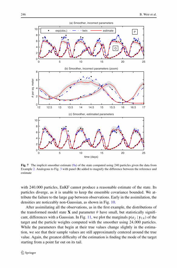
All the parameter estimates, except EnKF, are able to cross both bifurcations sepa-rating the initial approximation and true parameters. The results of the implicit meth-ods are listed for different numbers of particles in Table 4. Figure 7 compares thereference solution and the smoother estimate (9a) of the state when (a, b) a is keptfixed at the incorrect initial guess and (c) a is estimated. In both cases, we use 240 par-ticles. The failure of the state estimate in (a) is most evident at the peaks of the prey.We plot a magnified view of one peak in frame (b). Between observations, the modeldrift drives the prey toward its value of 6 at the incorrect parameters (see Fig. 6a). Wefix this deficiency by estimating parameters in frame (c), resulting in a state estimatewhose oscillations are within the high-probability regions of the true invariant mea-sure (see Fig. 6b). In Fig. 8, we plot the state estimates of EnKF, SIR, and the implicitfilter. The corresponding parameter estimates for the implicit filter (see Fig. 9) showgood agreement with both the reference parameters and the smoother estimate. Even

246 B. Weir et al.

Fig. 7 The implicit smoother estimate (9a) of the state computed using 240 particles given the data fromExample 2. Analogous to Fig. 3 with panel (b) added to magnify the difference between the reference andestimate

with 240,000 particles, EnKF cannot produce a reasonable estimate of the state. Itsparticles diverge, as it is unable to keep the ensemble covariance bounded. We at-tribute the failure to the large gap between observations. Early in the assimilation, thedensities are noticeably non-Gaussian, as shown in Fig. 10.

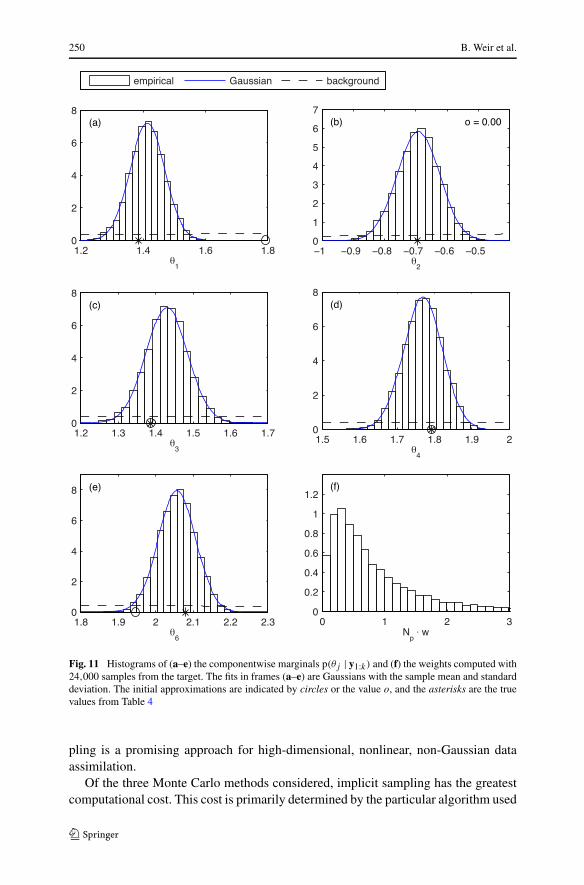
After assimilating all the observations, as in the first example, the distributions ofthe transformed model state X and parameter θ have small, but statistically signifi-cant, differences with a Gaussian. In Fig. 11, we plot the marginals p(aj | y1:k) of thetarget and the particle weights computed with the smoother using 24,000 particles.While the parameters that begin at their true values change slightly in the estima-tion, we see that their sample values are still approximately centered around the truevalue. Again, the greatest difficulty of the estimation is finding the mode of the targetstarting from a point far out on its tail.


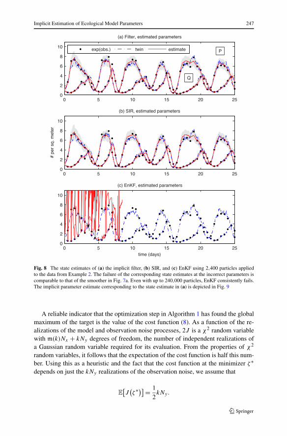
Fig. 8 The state estimates of (a) the implicit filter, (b) SIR, and (c) EnKF using 2,400 particles appliedto the data from Example 2. The failure of the corresponding state estimates at the incorrect parameters iscomparable to that of the smoother in Fig. 7a. Even with up to 240,000 particles, EnKF consistently fails.The implicit parameter estimate corresponding to the state estimate in (a) is depicted in Fig. 9

A reliable indicator that the optimization step in Algorithm 1 has found the globalmaximum of the target is the value of the cost function (8). As a function of the re-alizations of the model and observation noise processes, 2J is a χ2 random variablewith m(k)Nx + kNy degrees of freedom, the number of independent realizations ofa Gaussian random variable required for its evaluation. From the properties of χ2

random variables, it follows that the expectation of the cost function is half this num-ber. Using this as a heuristic and the fact that the cost function at the minimizer ζ ∗depends on just the kNy realizations of the observation noise, we assume that

E[J(ζ ∗)] = 1

2kNy.

248 B. Weir et al.

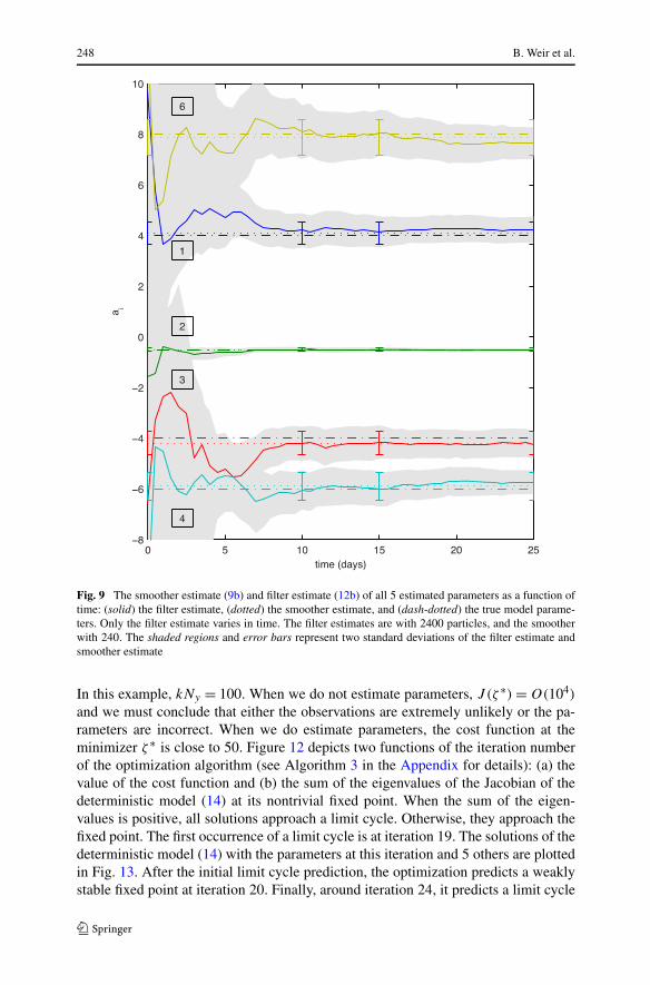
Fig. 9 The smoother estimate (9b) and filter estimate (12b) of all 5 estimated parameters as a function oftime: (solid) the filter estimate, (dotted) the smoother estimate, and (dash-dotted) the true model parame-ters. Only the filter estimate varies in time. The filter estimates are with 2400 particles, and the smootherwith 240. The shaded regions and error bars represent two standard deviations of the filter estimate andsmoother estimate

In this example, kNy = 100. When we do not estimate parameters, J (ζ ∗) = O(104)

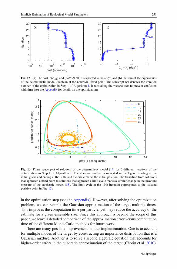
and we must conclude that either the observations are extremely unlikely or the pa-rameters are incorrect. When we do estimate parameters, the cost function at theminimizer ζ ∗ is close to 50. Figure 12 depicts two functions of the iteration numberof the optimization algorithm (see Algorithm 3 in the Appendix for details): (a) thevalue of the cost function and (b) the sum of the eigenvalues of the Jacobian of thedeterministic model (14) at its nontrivial fixed point. When the sum of the eigen-values is positive, all solutions approach a limit cycle. Otherwise, they approach thefixed point. The first occurrence of a limit cycle is at iteration 19. The solutions of thedeterministic model (14) with the parameters at this iteration and 5 others are plottedin Fig. 13. After the initial limit cycle prediction, the optimization predicts a weaklystable fixed point at iteration 20. Finally, around iteration 24, it predicts a limit cycle


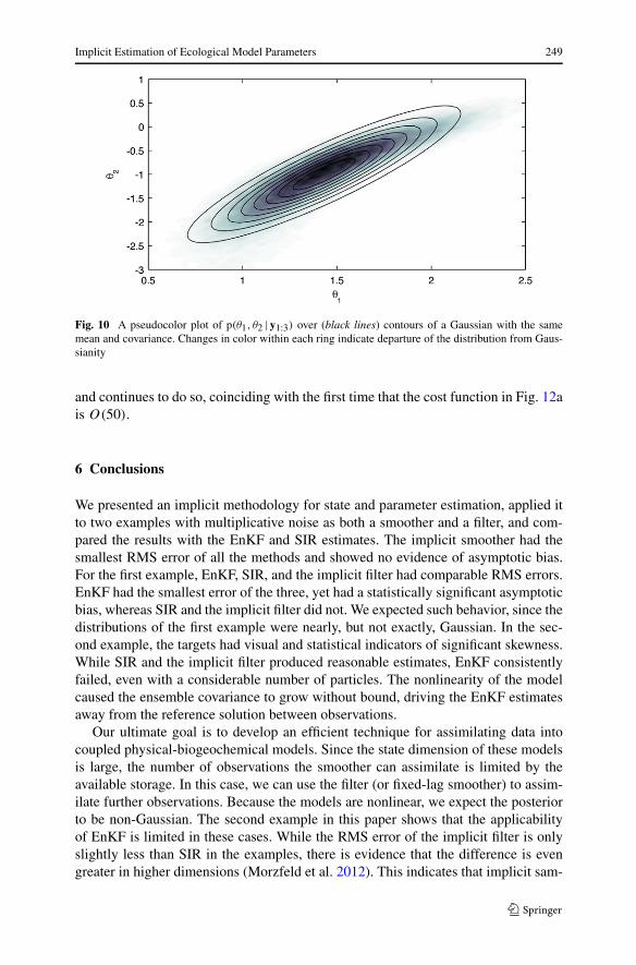
Fig. 10 A pseudocolor plot of p(θ1, θ2 |y1:3) over (black lines) contours of a Gaussian with the samemean and covariance. Changes in color within each ring indicate departure of the distribution from Gaus-sianity

and continues to do so, coinciding with the first time that the cost function in Fig. 12ais O(50).

6 Conclusions

We presented an implicit methodology for state and parameter estimation, applied itto two examples with multiplicative noise as both a smoother and a filter, and com-pared the results with the EnKF and SIR estimates. The implicit smoother had thesmallest RMS error of all the methods and showed no evidence of asymptotic bias.For the first example, EnKF, SIR, and the implicit filter had comparable RMS errors.EnKF had the smallest error of the three, yet had a statistically significant asymptoticbias, whereas SIR and the implicit filter did not. We expected such behavior, since thedistributions of the first example were nearly, but not exactly, Gaussian. In the sec-ond example, the targets had visual and statistical indicators of significant skewness.While SIR and the implicit filter produced reasonable estimates, EnKF consistentlyfailed, even with a considerable number of particles. The nonlinearity of the modelcaused the ensemble covariance to grow without bound, driving the EnKF estimatesaway from the reference solution between observations.

Our ultimate goal is to develop an efficient technique for assimilating data intocoupled physical-biogeochemical models. Since the state dimension of these modelsis large, the number of observations the smoother can assimilate is limited by theavailable storage. In this case, we can use the filter (or fixed-lag smoother) to assim-ilate further observations. Because the models are nonlinear, we expect the posteriorto be non-Gaussian. The second example in this paper shows that the applicabilityof EnKF is limited in these cases. While the RMS error of the implicit filter is onlyslightly less than SIR in the examples, there is evidence that the difference is evengreater in higher dimensions (Morzfeld et al. 2012). This indicates that implicit sam-

250 B. Weir et al.

Fig. 11 Histograms of (a–e) the componentwise marginals p(θj | y1:k) and (f) the weights computed with24,000 samples from the target. The fits in frames (a–e) are Gaussians with the sample mean and standarddeviation. The initial approximations are indicated by circles or the value o, and the asterisks are the truevalues from Table 4

pling is a promising approach for high-dimensional, nonlinear, non-Gaussian dataassimilation.

Of the three Monte Carlo methods considered, implicit sampling has the greatestcomputational cost. This cost is primarily determined by the particular algorithm used


Fig. 12 (a) The cost J (ζ(k)) and (dotted) 50, its expected value at ζ∗, and (b) the sum of the eigenvaluesof the deterministic model Jacobian at the nontrivial fixed point. The subscript (k) denotes the iterationnumber of the optimization in Step 1 of Algorithm 1. It runs along the vertical axis to prevent confusionwith time (see the Appendix for details on the optimization)

Fig. 13 Phase space plot of solutions of the deterministic model (14) for 6 different iterations of theoptimization in Step 1 of Algorithm 1. The iteration number is indicated in the legend, starting at theinitial guess and ending at the 30th, and the circle marks the initial position. The transition from solutionsthat approach a fixed point to solutions that approach a limit cycle marks a similar change in the invariantmeasure of the stochastic model (15). The limit cycle at the 19th iteration corresponds to the isolatedpositive point in Fig. 12b

in the optimization step (see the Appendix). However, after solving the optimizationproblem, we can sample the Gaussian approximation of the target multiple times.This improves the computation time per particle, yet may reduce the accuracy of theestimate for a given ensemble size. Since this approach is beyond the scope of thispaper, we leave a detailed comparison of the approximation error versus computationtime of the different Monte Carlo methods for future work.

There are many possible improvements to our implementation. One is to accountfor multiple modes of the target by constructing an importance distribution that is aGaussian mixture. Another is to solve a second algebraic equation that accounts forhigher-order errors in the quadratic approximation of the target (Chorin et al. 2010).

252 B. Weir et al.

Finally, we expect the kernel density estimate for the parameters to have a significanteffect on the efficiency of the implicit filter. The optimal bandwidth (Sheather andJones 1991) and the use of kernel density methods with particle filters in general aregrowing and promising topics of research (Silverman 1986).

Acknowledgements The authors thank Dr. Ethan Atkins, Professor Alexandre Chorin, and Dr. MatthiasMorzfeld for their invaluable contribution to the research and presentation of the results in this paper. Wethank Linda Lamb as well for her detailed proofreading. This work was supported by the National ScienceFoundation, Division of Ocean Sciences, Collaboration in Mathematical Geosciences award #0934956.

Appendix: The Optimization Problem

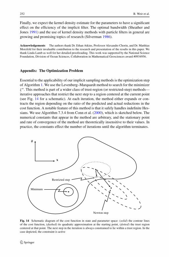
Essential to the applicability of our implicit sampling methods is the optimization stepof Algorithm 1. We use the Levenberg–Marquardt method to search for the minimizerζ ∗. This method is part of a wider class of trust-region (or restricted-step) methods—iterative approaches that restrict the next step to a region centered at the current point(see Fig. 14 for a schematic). At each iteration, the method either expands or con-tracts the region depending on the ratio of the predicted and actual reductions in thecost function. A notable feature of this method is that it safely handles indefinite Hes-sians. We use Algorithm 7.3.4 from Conn et al. (2000), which is sketched below. Thenumerical constants that appear in the method are arbitrary, and the stationary pointand rate of convergence of the method are theoretically insensitive to their values. Inpractice, the constants effect the number of iterations until the algorithm terminates.

Fig. 14 Schematic diagram of the cost function in state and parameter space: (solid) the contour linesof the cost function, (dashed) its quadratic approximation at the starting point, (dotted) the trust regioncentered at that point. The next step in the iteration is always constrained to lie within a trust region. In thecase depicted, the constraint is active


Algorithm 3 (Levenberg–Marquardt) Let the subscript (k) denote the iteration num-ber and suppose we have some initial guess ζ(0) and radius ε(0).

1 At the current point ζ(k), compute the cost function, its gradient, and Hessian:

J(k) = J (ζ(k)), g(k) = ∇J (ζ(k)), H(k) = H(ζ(k)).

2 Find the proposed increment �ζ that minimizes the quadratic approximation at thecurrent point, defined such that

K(ζ(k) + �ζ) = J(k) + gT(k)�ζ + 1

2(�ζ)T H(k)�ζ,

constrained to the region where

(�ζ)T �ζ ≤ ε2(k).

For more details on the solution of quadratic programming problems, see themonograph of Conn et al. (2000).

3 Compute the ratio of the actual reduction to predicted reduction of the function atthe proposed next step,

r = J (ζ(k)) − J (ζ(k) + �ζ)

K(ζ(k)) − K(ζ(k) + �ζ).

Update the trust region size based on r ,

ε(k+1) =⎧⎨⎩

ε(k)/2 if r < 1/4,

min(2ε(k), εM) if r > 3/4,

ε(k) otherwise,

where εM is a user specified maximum radius. Move to the next point only if itdecreases the cost function, i.e.,

ζ(k+1) ={

ζ(k) + �ζ if 0 < r,

ζ(k) otherwise.

Since the proposed increment �ζ minimizes K within the trust region, the denom-inator of the ratio r is always positive. Hence, the iteration remains at the currentstep if and only if the predicted step does not decrease the cost function.

4 Replace k with k + 1, and return to Step 1 until the norm of the gradient g(k) is lessthan a given value or we reach an upper bound of iterations.

The Derivatives of the Cost Function

The structure of the Hessian of J makes it possible to do these computations ef-ficiently even when the dimension of ζ is large. Since the residuals only depend on

254 B. Weir et al.

the previous and current model step, the Hessian has a single band running down itsdiagonal, corresponding to the state derivatives, full columns at its far-right side, andfull rows at its bottom, both corresponding to the parameter derivatives. We need onlystore the diagonal, subdiagonals, and bottom rows because the Hessian is symmetric.This representation grows linearly in the number of variables, as opposed to quadrati-cally for the full representation. If the model equations are a discretization of a partialdifferential equation, we lose this special structure, but numerous libraries exist foroptimization when the Hessian is sparse. Thus, the Hessian has the block form

H =[

Hxx Hxθ

Hθx Hθθ

],

where Hxx is a band matrix, and Hθx = HTxθ since we assume J is smooth.

To simplify notation, define the (column) vector of residuals

ρ = (em(l)+1:m(l+k),dl+1:l+k).

The cost function, its gradient, and its Hessian are thus

J (ζ ) = 1

2ρT ρ, ∇J = (∇ρ)T ρ, H = (∇ρ)T (∇ρ) +

∑i

Hρiρi,

where Hρiis the Hessian of the ith element of ρ. We use the Gauss–Newton approx-

imation of the Hessian,

H = (∇ρ)T (∇ρ).

Since the goal of the optimization is to make the norm of the residuals small, weexpect the neglected terms to be small as well (Fletcher 1987). The derivatives ofthe cost function in the unconstrained variables follow from an application of thechain rule. An added benefit of the Gauss–Newton approximation is that it is alwayspositive semi-definite. Hence, we can stop the optimization at any iteration, and it isstill possible to sample a Gaussian whose covariance matrix is the Moore–Penrosepseudoinverse of the Hessian.

The nonzero derivatives of the model noise are

∂em/∂xm = (√

τG)−1,

∂em/∂xm−1 = −(√

τG)−1[I + τ ∂f (xm−1, θ)/∂xm−1],

∂em/∂θ = −(√

τG)−1[τ ∂f (xm−1, θ)/∂θ],

and the derivative of the observation noise is

∂dn/∂xm(n) = (√

R)−1∂h(xm(n))/∂xm(n).

The state derivatives of the Lotka–Volterra model equations (14) are

∂φ

∂u=

[a1 + 2a2p + a3q/(1 + a7p)2 a3p/(1 + a7p)

a6q/(1 + a7p)2 a4 + 2a5q + a6p/(1 + a7p)

],


and the derivatives for each parameter are

∂φ

∂a1=

[p

0

],

∂φ

∂a2=

[p2

0

],

∂φ

∂a3=

[pq/(1 + a7p)

0

],

∂φ

∂a4=

[0q

],

∂φ

∂a5=

[0q2

],

∂φ

∂a6=

[0

pq/(1 + a7p)

],

and

∂φ

∂a7=

[−a3p2q/(1 + a7p)2

−a6p2q/(1 + a7p)2

].

Since the observation functions considered are linear, their Jacobians are identical tothe functions.

References

Andrieu, C., Doucet, A., & Holenstein, R. (2010). Particle Markov chain Monte Carlo methods. J. R. Stat.Soc. Ser. B Stat. Methodol., 72, 269–342.

de Angelis, D. L. (1975). Estimates of predator-prey limit cycles. Bull. Math. Biol., 37, 291–299.Arnold, L. (1998). Random dynamical systems. Berlin: Springer.Arulampalam, M. S., Maskell, S., Gordon, N., & Clapp, T. (2002). A tutorial on particle filters for online

nonlinear/non-Gaussian Bayesian tracking. IEEE Trans. Signal Process., 50, 174–188.Brauer, F., & Castillo-Chavez, C. (2012). Mathematical models in population biology and epidemiology

(2nd ed.). New York: Springer.Chorin, A. J., & Hald, O. H. (2009). Stochastic tools in mathematics and science (2nd ed.). Dordrecht:

Springer.Chorin, A. J., & Tu, X. (2009). Implicit sampling for particle filters. Proc. Natl. Acad. Sci. USA, 106,

17,249–17,254.Chorin, A. J., Morzfeld, M., & Tu, X. (2010). Implicit particle filters for data assimilation. Commun. Appl.

Math. Comput. Sci., 5, 221–240.Conn, A. R., Gould, N. I. M., & Toint, P. L. (2000). Trust-region methods. Philadelphia: SIAM.Cossarini, G., Lermusiaux, P. F. J., & Solidoro, C. (2009). Lagoon of Venice ecosystem: seasonal dynam-

ics and environmental guidance with uncertainty analyses and error subspace data assimilation. J.Geophys. Res., 114. doi:10.1029/2008JC005080.

Courtier, P., & Talagrand, O. (1987). Variational assimilation of meteorological observations with theadjoint vorticity equation. II: Numerical results. Q. J. R. Meteorol. Soc., 113, 1329–1347.

Dempster, A. P., Laird, N. M., & Rubin, D. B. (1977). Maximum likelihood from incomplete data via theEM algorithm. J. R. Stat. Soc. Ser. B Stat. Methodol., 39, 1–38.

Doron, M., Brasseur, P., & Brankart, J.-M. (2011). Stochastic estimation of biogeochemical parameters ofa 3D ocean coupled physical-biogeochemical model: twin experiments. J. Mar. Syst., 87, 194–207.

Doucet, A., Godsill, S., & Andrieu, C. (2000). On sequential Monte Carlo sampling methods for Bayesianfiltering. Statist. Comput., 10, 197–208.

Doucet, A., de Freitas, N., & Gordon, N. (2001). Sequential Monte Carlo methods in practice. New York:Springer.

Dowd, M. (2006). A sequential Monte Carlo approach for marine ecological prediction. Environmetrics,17, 435–455.

Dowd, M. (2007). Bayesian statistical data assimilation for ecosystem models using Markov chain MonteCarlo. J. Mar. Syst., 68, 439–456.

Dowd, M. (2011). Estimating parameters for a stochastic dynamic marine ecological system. Environ-metrics, 22, 501–515.

Efron, B. (1979). Bootstrap methods: another look at the jackknife. Ann. Statist., 7, 1–26.Efron, B. (2003). Second thoughts on the bootstrap. Statist. Sci., 18, 135–140.Evensen, G. (2009). Data assimilation: the ensemble Kalman filter (2nd ed.). Dordrecht: Springer.

http://dx.doi.org/10.1029/2008JC005080

256 B. Weir et al.

Fasham, M. J. R., Ducklow, H. W., & McKelvie, S. M. (1990). A nitrogen-based model of planktondynamics in the oceanic mixed layer. J. Mar. Res., 48, 591–639.

Fletcher, R. (1987). Practical methods of optimization (2nd ed.). Chichester: Wiley.Friedrichs, M. A. M. (2002). Assimilation of JGOFS EqPac and SeaWIFS data into a marine ecosystem

model of the central equatorial Pacific Ocean. Deep-Sea Res., Part 2, 49, 289–319.Friedrichs, M. A. M., Dusenberry, J. A., Anderson, L. A., Armstrong, R. A., Chai, F., Christian, J. R.,

Doney, S. C., Dunne, J., Fujii, M., Hood, R., McGillicuddy, D. J. Jr., Moore, J. K., Schartau,M., Spitz, Y. H., & Wiggert, J. D. (2007). Assessment of skill and portability in regional marinebiogeochemical models: role of multiple planktonic groups. J. Geophys. Res., 112. doi:10.1029/2006JC003852.

Geweke, J. (1989). Bayesian inference in econometric models using Monte Carlo integration. Economet-rica, 57, 1317–1339.

Gilks, W. R., & Berzuini, C. (2001). Following a moving target—Monte Carlo inference for dynamicBayesian models. J. R. Stat. Soc. Ser. B Stat. Methodol., 63, 127–146.

Golightly, A., & Wilkinson, D. J. (2011). Bayesian parameter inference for stochastic biochemical networkmodels using Markov chain Monte Carlo. J. R. Soc. Interface, 1, 807–820.

Gordon, N. J., Salmond, D. J., & Smith, A. F. M. (1993). Novel approach to nonlinear/non-GaussianBayesian state estimation. IEE Proc. F, 140, 107–113.

Gregg, W. W. (2008). Assimilation of SeaWIFS ocean chlorophyll data into a three-dimensional globalocean model. J. Mar. Syst., 69, 205–225.

Holling, C. S. (1959). Some characteristics of simple types of predation and parasitism. Can. Entomol.,91, 385–398.

Hurtt, G. C., & Armstrong, R. A. (1996). A pelagic ecosystem model calibrated with BATS data. Deep-SeaRes., Part 2, 43, 653–683.

Hurtt, G. C., & Armstrong, R. A. (1999). A pelagic ecosystem model calibrated with BATS and OWSIdata. Deep-Sea Res., Part 1, 46, 27–61.

Ionides, E. L., Bretó, C., & King, A. A. (2006). Inference for nonlinear dynamical systems. Proc. Natl.Acad. Sci. USA, 103, 18,438–18,443.

Johnson, K. A., & Goody, R. S. (2011). The original Michaelis constant: translation of the 1913 Michaelis-Menten paper. Biochemistry, 50, 8264–8269.

Kitagawa, G. (1996). Monte Carlo filter and smoother for non-Gaussian nonlinear state space models. J.Comput. Graph. Statist., 5, 1–25.

Kivman, G. A. (2003). Sequential parameter estimation for stochastic systems. Nonlinear Process. Geo-phys., 10, 253–259.

Kloeden, P. E., & Platen, E. (1999). Numerical solution of stochastic differential equations. Berlin:Springer.

Lawson, L. M., Spitz, Y. H., Hofmann, E. E., & Long, R. B. (1995). A data assimilation technique appliedto a predator-prey model. Bull. Math. Biol., 57, 593–617.

Lawson, L. M., Hofmann, E. E., & Spitz, Y. H. (1996). Time series sampling and data assimilation in asimple marine ecosystem model. Deep-Sea Res., Part 2, 43, 625–651.

van Leeuwen, P. J. (2009). Particle filtering in geophysical systems. Mon. Weather Rev., 137, 4089–4114.Lehmann, E. L., & Casella, G. (1998). Theory of point estimation (2nd ed.). New York: Springer.Liu, J., & West, M. (2001). Combined parameter and state estimation in simulation based filtering. In

A. Doucet, N. de Freitas, & N. Gordon (Eds.), Sequential Monte Carlo methods in practice (pp.197–217). New York: Springer.

Longhurst, A. (1995). Seasonal cycles of pelagic production and consumption. Prog. Oceanogr., 36, 77–167.

Lorenz, E. N. (1963). Deterministic nonperiodic flow. J. Atmospheric Sci., 20, 130–141.Losa, S. N., Kivman, G. A., Schroter, J., & Wenzel, M. (2003). Sequential weak constraint parameter

estimation in an ecosystem model. J. Mar. Syst., 43, 31–49.Marjoram, P., Molitor, J., Plagnol, V., & Tavaré, S. (2003). Markov chain Monte Carlo without likelihoods.

Proc. Natl. Acad. Sci. USA, 100, 15,324–15,328.Matear, R. J. (1995). Parameter optimization and analysis of ecosystem models using simulated annealing:

a case study at Station P. J. Mar. Res., 53, 571–607.May, R. M. (1972). Limit cycles in predator-prey communities. Science, 177, 900–902.McLachlan, G. J., & Krishnan, T. (2008). The EM algorithm and extensions (2nd ed.). Hoboken: Wiley.Metropolis, N., Rosenbluth, A. W., Teller, A. H., & Teller, E. (1953). Equations of state calculations by

fast computing machines. J. Chem. Phys., 21, 1087–1092.

http://dx.doi.org/10.1029/2006JC003852

http://dx.doi.org/10.1029/2006JC003852


Michaelis, L., & Menten, M. L. (1913). Die Kinetik der Invertinwirkung. Biochem. Z., 49, 333–369.Miller, R. N., Carter, E. F. Jr., & Blue, S. T. (1999). Data assimilation into nonlinear stochastic models.

Tellus A, 51, 167–194.Morzfeld, M., & Chorin, A. J. (2012). Implicit particle filtering for models with partial noise, and an

application to geomagnetic data assimilation. Nonlinear Process. Geophys., 19, 365–382.Morzfeld, M., Tu, X., Atkins, E., & Chorin, A. J. (2012). A random map implementation of implicit filters.

J. Comput. Phys., 231, 2049–2066.Newberger, P. A., Allen, J. S., & Spitz, Y. H. (2003). Analysis and comparison of three ecosystem models.

J. Geophys. Res., 108. doi:10.1029/2001JC001182.Øksendal, B. K. (2003). Stochastic differential equations: an introduction with applications (6th ed.).

Berlin: Springer.Raftery, A. E., & Bao, L. (2010). Estimating and projecting trends in HIV/AIDS generalized epidemics

using incremental mixture importance sampling. Biometrics, 66, 1162–1173.Ripley, B. (1987). Stochastic simulation. New York: Wiley.Robinson, A. R., & Lermusiaux, P. F. J. (2002). Data assimilation for modeling and predicting coupled

physical-biological interactions in the sea. In A. R. Robinson, J. J. McCarthy, & B. J. Rothschild(Eds.), Biological-physical interactions in the sea. The sea (Vol. 12, pp. 475–536). New York: Wiley.

Sapsis, T. P., & Lermusiaux, P. F. J. (2009). Dynamically orthogonal field equations for continuous stochas-tic dynamical systems. Physica D, 238, 2347–2360.

Sapsis, T. P., & Lermusiaux, P. F. J. (2012). Dynamical criteria for the evolution of the stochastic dimen-sionality in flows with uncertainty. Physica D, 241, 60–76.

Sheather, S. J., & Jones, M. C. (1991). A reliable data-based bandwidth selection method for kernel densityestimation. J. R. Stat. Soc. Ser. B, 53, 683–690.

Sheskin, D. J. (2011). Handbook of parametric and nonparametric statistical procedures (5th ed.). BocaRaton: Chapman & Hall/CRC.

Silverman, B. W. (1986). Density estimation for statistics and data analysis. London: Chapman &Hall/CRC.

Simon, E., & Bertino, L. (2012). Gaussian anamorphosis extension of the DEnKF for combined state andparameter estimation: application to a 1D ocean ecosystem model. J. Mar. Syst., 89, 1–18.

Snyder, C., Bengtsson, T., Bickel, P., & Anderson, J. (2008). Obstacles to high-dimensional particle filter-ing. Mon. Weather Rev., 136, 4629–4640.

Spitz, Y. H., Moisan, J. R., & Abbott, M. R. (2001). Configuring an ecosystem model using data from theBermuda Atlantic Time Series (BATS). Deep-Sea Res., Part 2, 48, 1733–1768.

Sugie, J., Kohno, R., & Miyazaki, R. (1997). On a predator-prey system of Holling type. Proc. Amer. Math.Soc., 125, 2041–2050.

Talagrand, O., & Courtier, P. (1987). Variational assimilation of meteorological observations with theadjoint vorticity equation. I: Theory. Q. J. R. Meteorol. Soc., 113, 1311–1328.

Vallino, J. J. (2000). Improving marine ecosystem models: use of data assimilation and mesocosm experi-ments. J. Mar. Res., 58, 117–164.

Wilkinson, D. J. (2010). Parameter inference for stochastic kinetic models of bacterial gene regulation: aBayesian approach to systems biology. In J. M. Bernardo, M. J. Bayarri, J. O. Berger, A. P. Dawid,D. Heckerman, A. F. P. Smith, & M. West (Eds.), Bayesian statistics: Vol. 9. Proceedings of the ninthValencia international meeting (pp. 679–706). Oxford: Oxford University Press.

Zakai, M. (1969). On the optimal filtering of diffusion processes. Probab. Theory Related Fields, 11, 230–243.

Zhao, L., Wei, H., Xu, Y., & Feng, S. (2005). An adjoint data assimilation approach for estimating param-eters in a three-dimensional ecosystem model. Ecol. Model., 186, 234–249.

http://dx.doi.org/10.1029/2001JC001182

implicit estimation of ecological model parameters

Documents