Brigham Young UniversityBYU ScholarsArchive

All Faculty Publications

2014-08-09

Implementing Dubins Airplane Paths on Fixed-wing UAVsTimothy McLainMechanical Engineering Department, Brigham Young University, mclain@byu.edu

Randall W. BeardDepartment of Electrical Engineering, Brigham Young University

See next page for additional authors

Follow this and additional works at: https://scholarsarchive.byu.edu/facpubPart of the Mechanical Engineering Commons

Original Publication CitationOwen, M, Beard, R. and McLain, T. Implementing Dubins Airplane Paths on Fixed-wing UAVs,Contributed chapter to the Handbook of Unmanned Aerial Vehicles, Springer, ch. 68, pp.1677-1701, 2014.

This Book Chapter is brought to you for free and open access by BYU ScholarsArchive. It has been accepted for inclusion in All Faculty Publications byan authorized administrator of BYU ScholarsArchive. For more information, please contact scholarsarchive@byu.edu, ellen_amatangelo@byu.edu.

BYU ScholarsArchive CitationMcLain, Timothy; Beard, Randall W.; and Owen, Mark, "Implementing Dubins Airplane Paths on Fixed-wing UAVs" (2014). AllFaculty Publications. 1900.https://scholarsarchive.byu.edu/facpub/1900

AuthorsTimothy McLain, Randall W. Beard, and Mark Owen

This book chapter is available at BYU ScholarsArchive: https://scholarsarchive.byu.edu/facpub/1900

68Implementing Dubins Airplane Pathson Fixed-Wing UAVs!

Mark Owen, Randal W. Beard, and Timothy W. McLain

Contents68.1 Introduction . . . . . . . . . . . . . . . . . . . . . . . . . . . . . . . . . . . . . . . . . . . . . . . . . . . . . . . . . . . . . . . . . . . . . . . . . . . . . . . . . 167868.2 Equations of Motion for the Dubins Airplane . . . . . . . . . . . . . . . . . . . . . . . . . . . . . . . . . . . . . . . . . . . . . 168068.3 3D Vector-Field Path Following. . . . . . . . . . . . . . . . . . . . . . . . . . . . . . . . . . . . . . . . . . . . . . . . . . . . . . . . . . . . 1682

68.3.1 Vector-Field Methodology . . . . . . . . . . . . . . . . . . . . . . . . . . . . . . . . . . . . . . . . . . . . . . . . . . . . . . . . 168368.3.2 Straight-Line Paths . . . . . . . . . . . . . . . . . . . . . . . . . . . . . . . . . . . . . . . . . . . . . . . . . . . . . . . . . . . . . . . . 168468.3.3 Helical Paths . . . . . . . . . . . . . . . . . . . . . . . . . . . . . . . . . . . . . . . . . . . . . . . . . . . . . . . . . . . . . . . . . . . . . . . 1686

68.4 Minimum-Distance Airplane Paths . . . . . . . . . . . . . . . . . . . . . . . . . . . . . . . . . . . . . . . . . . . . . . . . . . . . . . . . 168768.4.1 Dubins Car Paths . . . . . . . . . . . . . . . . . . . . . . . . . . . . . . . . . . . . . . . . . . . . . . . . . . . . . . . . . . . . . . . . . . 168868.4.2 Dubins Airplane Paths . . . . . . . . . . . . . . . . . . . . . . . . . . . . . . . . . . . . . . . . . . . . . . . . . . . . . . . . . . . . 169068.4.3 Path Manager for Dubins Airplane . . . . . . . . . . . . . . . . . . . . . . . . . . . . . . . . . . . . . . . . . . . . . . . 169668.4.4 Simulation Results. . . . . . . . . . . . . . . . . . . . . . . . . . . . . . . . . . . . . . . . . . . . . . . . . . . . . . . . . . . . . . . . . 1696

68.5 Conclusion . . . . . . . . . . . . . . . . . . . . . . . . . . . . . . . . . . . . . . . . . . . . . . . . . . . . . . . . . . . . . . . . . . . . . . . . . . . . . . . . . . 1697References . . . . . . . . . . . . . . . . . . . . . . . . . . . . . . . . . . . . . . . . . . . . . . . . . . . . . . . . . . . . . . . . . . . . . . . . . . . . . . . . . . . . . . . . . . 1699

!Contributed Chapter to the Springer Handbook for Unmanned Aerial Vehicles

M. OwenSandia National Labs, Albuquerque, NM, USA

R.W. Beard (!)Electrical and Computer Engineering Department, Brigham Young University,Provo, UT, USAe-mail: beard@byu.edu

T.W. McLainMechanical Engineering Department, Brigham Young University, Provo, UT, USAe-mail: mclain@byu.edu

K.P. Valavanis, G.J. Vachtsevanos (eds.), Handbook of Unmanned Aerial Vehicles,DOI 10.1007/978-90-481-9707-1 120,© Springer Science+Business Media Dordrecht 2014

1677

1678 M. Owen et al.

AbstractA well-known path-planning technique for mobile robots or planar aerial vehiclesis to use Dubins paths, which are minimum-distance paths between two con-figurations subject to the constraints of the Dubins car model. An extensionof this method to a three-dimensional Dubins airplane model has recently beenproposed. This chapter builds on that work showing a complete architecture forimplementing Dubins airplane paths on small fixed-wing UAVs. The existingDubins airplane model is modified to be more consistent with the kinematicsof a fixed-wing aircraft. The chapter then shows how a recently proposedvector-field method can be used to design a guidance law that causes the Dubinsairplane model to follow straight-line and helical paths. Dubins airplane pathsare more complicated than Dubins car paths because of the altitude component.Based on the difference between the altitude of the start and end configurations,Dubins airplane paths can be classified as low, medium, or high altitude gain.While for medium and high altitude gain there are many different Dubins airplanepaths, this chapter proposes selecting the path that maximizes the averagealtitude throughout the maneuver. The proposed architecture is implemented ona six degree-of-freedom Matlab/Simulink simulation of an Aerosonde UAV, andresults from this simulation demonstrate the effectiveness of the technique.

68.1 Introduction

Unmanned aerial vehicles (UAVs) are used for a wide variety of tasks that requirethe UAV to be flown from one particular pose (position and attitude) to another. Mostcommonly, UAVs are flown from their current position and heading angle to a newdesired position and heading angle. The ability to fly from one pose (or waypoint)to another is the fundamental building block upon which more sophisticated UAVnavigation capabilities are built. For UAV missions involving sensors, the ability toposition and orient the sensor over time is critically important. Example applicationsinclude wildlife observation and tracking, infrastructure monitoring (Rathinam et al.2005; Frew et al. 2004; Egbert and Beard 2011), communication relays (Frewet al. 2009), meteorological measurements (Elston et al. 2010), and aerial surveil-lance (Rahmani et al. 2010; Elston and Frew 2008; Spry et al. 2005). Positioningand orienting the sensor is accomplished in part by planning and following pathsthrough or above the sensing domain. Two-dimensional (2D) path planning andfollowing at a constant altitude through unobstructed airspace is common, but asmission scenarios become increasingly sophisticated by requiring flight in three-dimensional (3D) terrain, the need for full 3D planning and guidance algorithms isbecoming increasingly important.

For a vehicle that moves in a 2D plane at constant forward speed with afinite turn-rate constraint, the minimum-distance path between two configurationsis termed a Dubins path. The initial and final configurations are defined by a2D position in the plane of motion and an orientation. It has been shown thatthe optimal Dubins path in the absence of wind is composed of a constantradius turn, followed by a straight-line path, followed by another constant radius

68 Implementing Dubins Airplane Paths on Fixed-Wing UAVs 1679

turn (Dubins 1957). A vehicle that follows Dubins paths is often termed a Dubinscar. There have been a wide variety of path-planning techniques proposed for mobilerobots based on the Dubins car model (e.g., Hanson et al. 2011; Balluchi et al.1996; Anderson and Milutinovic 2011; Karaman and Frazzoli 2011; Cowlagi andTsiotras 2009; Yong and Barth 2006). The Dubins car model has also been usedextensively for UAV applications by constraining the air vehicle to fly at a constantaltitude (e.g., Yu and Beard 2013; Sujit et al. 2007; Yang and Kapila 2002; Shimaet al. 2007).

The Dubins car model was recently extended to three dimensions to create theDubins airplane model, where in addition to turn-rate constraints, a climb-rateconstraint was added (Hosak and Ghose 2010; Chitsaz and LaValle 2007; Rahmaniet al. 2010). Minimum-distance paths for the Dubins airplane were also derivedin Chitsaz and LaValle (2007), using the Pontryagin minimum principle (Lewis1986). However, in Chitsaz and LaValle (2007) some practical issues were notconsidered, leaving a gap between the theory and implementation on actual UAVs.The purpose of this chapter is to fill that gap. In particular, alternative equations ofmotion for the Dubins airplane model that include airspeed, flight-path angle, andbank angle are given. The kinematic equations of motion presented in this chapterare standard in the aerospace literature. The chapter also describes how to implementDubins airplane paths using low-level autopilot loops, vector-field guidance laws forfollowing straight lines and helices, and mode switching between the guidance laws.

In addition to the complexity of a third dimension of motion, Dubins airplanepaths are more complicated than Dubins car paths. In particular, when the altitudecomponent of the path falls within a specific range, there are an infinite numberof paths that satisfy the minimum-distance objective. This chapter also proposesspecific choices for paths that make practical sense for many UAV missionscenarios. Specifically, the path that also maximizes the average altitude of the pathis selected.

The software architecture proposed in this chapter is similar to that discussedin Beard and McLain (2012) and is shown in Fig. 68.1. At the lowest level is thefixed-wing UAV. A state estimator processes sensors and produces the estimatesof the state required for each of the higher levels. A low-level autopilot acceptsairspeed, flight-path angle, and bank angle commands. The commands for the low-level autopilot are produced by a vector-field guidance law for following eitherstraight-line paths or helical paths. The minimum-distance Dubins airplane pathbetween two configurations is computed by the path manager, which also switchesbetween commanding straight-line paths and helical paths.

This chapter will not discuss state estimation using the available sensors, butthe interested reader is referred to Beard and McLain (2012) and other publicationson state estimation for UAVs (see, e.g., Mahony et al. 2008; Misawa and Hedrick1989; Brunke and Campbell 2004). Section 68.2 briefly describes assumptions onthe unmanned aircraft and how the low-level autopilot is configured to produce theDubins airplane kinematic model. Section 68.3 describes the vector-field guidancestrategy used in this chapter for following both straight lines and helices. The Dubinsairplane paths and the path manager used to follow them are discussed in Sect. 68.4.Section 68.5 offers concluding remarks.

1680 M. Owen et al.

Dubins Path Manager

Vector Field Guidance

Unmanned Aircraft

Configuration Waypoints:(position, heading)

Sensors

Position error

Tracking error

Throttle Control Surfaces

State Estimator

Path definition: straight-line, or

helix

Airspeed Flight path angle

Bank angle Low Level Autopilot

Fig. 68.1 Flight control architecture proposed in this chapter

68.2 Equations of Motion for the Dubins Airplane

Unmanned aircraft, particularly smaller systems, fly at relatively low airspeedscausing wind to have a significant effect on their performance. Since wind effectsare not known prior to the moment they act on an aircraft, they are typically treatedas a disturbance to be rejected in real time by the flight control system, rather thanbeing considered during the path planning. It has been shown that vector-field-basedpath following methods, such as those employed in this chapter, are particularlyeffective at rejecting wind disturbances (Nelson et al. 2007). Treating wind as adisturbance also allows paths to be planned relative to the inertial environment,which is important as UAVs are flown in complex 3D terrain. Accordingly, whenthe Dubins airplane model is used for path planning, the effects of wind are notaccounted for when formulating the equations of motion. In this case, the airspeedV is the same as the groundspeed, the heading angle is the same as the courseangle (assuming zero sideslip angle), and the flight-path angle ! is the same as theair-mass-referenced flight-path angle (Beard and McLain 2012).

Figure 68.2 depicts a UAV flying with airspeed V , heading angle , andflight-path angle ! . Denoting the inertial position of the UAV as .rn; re; rd />, thekinematic relationship between the inertial velocity, v D .Prn; Pre; Prd />, and theairspeed, heading angle, and flight-path angle can be easily visualized as

0

@PrnPrePrd

1

A D

0

@V cos cos !V sin cos !!V sin !

1

A ;

where V D kvk.

68 Implementing Dubins Airplane Paths on Fixed-Wing UAVs 1681

Flight path projected onto ground

horizontal componentof airspeed vector

ki (down)

ji (east)

ii (north)

ii

V cosγ

rn = V cosψ cosγ re = V sinψ cosγ

−rd = V sinγ˙

ψ

γ

v

Fig. 68.2 Graphical representation of aircraft kinematic model

This chapter assumes that a low-level autopilot regulates the airspeed V to aconstant commanded value V c , the flight-path angle ! to the commanded flight-pathangle ! c , and the bank angle " to the commanded bank angle "c . In addition, thedynamics of the flight-path angle and bank angle loops are assumed to be sufficientlyfast that they can be ignored for the purpose of path following. The relationshipbetween the heading angle and the bank angle " is given by the coordinated turncondition (Beard and McLain 2012)

P D g

Vtan";

where g is the acceleration due to gravity.Under the assumption that the autopilot is well tuned and the airspeed, flight-path

angle, and bank angle states converge with the desired response to their commandedvalues, then the following kinematic model is a good description of the UAVmotion:

1682 M. Owen et al.

Prn D V cos cos ! c

Pre D V sin cos ! c (68.1)

Prd D !V sin ! c

P D g

Vtan"c:

Physical capabilities of the aircraft place limits on the achievable bank andflight-path angles that can be commanded. These physical limits on the aircraft arerepresented by the following constraints:

j"cj " N" (68.2)

j! cj " N! : (68.3)

The kinematic model given by (68.1) with the input constraints (68.2) and (68.3)will be referred to as the Dubins airplane. This model builds upon the modeloriginally proposed for the Dubins airplane in Chitsaz and LaValle (2007), which isgiven by

Prn D V cos

Pre D V sin (68.4)

Prd D u1 ju1j " 1P D u2 ju2j " 1:

Although (68.1) is similar to (68.4), it captures the aircraft kinematics withgreater accuracy and provides greater insight into the aircraft behavior and is moreconsistent with commonly used aircraft guidance models. Note, however, that (68.1)is only a kinematic model that does not include aerodynamics, wind effects, orengine/thrust limits. While it is not sufficiently accurate for low-level autopilotdesign, it is well suited for high-level path-planning and path-following controldesign. In-depth discussions of aircraft dynamic models can be found in Phillips(2010), Stevens and Lewis (2003), Nelson (1998) and Yechout et al. (2003).

68.3 3D Vector-Field Path Following

This section shows how to develop guidance laws to ensure that the kinematicmodel (68.1) follows straight-line and helical paths. Section 68.4 shows howstraight-line and helical paths are combined to produce minimum-distance pathsbetween start and end configurations.

68 Implementing Dubins Airplane Paths on Fixed-Wing UAVs 1683

68.3.1 Vector-Field Methodology

The guidance strategy will use the vector-field methodology proposed in Goncalveset al. (2010), and this section provides a brief overview. The path to be followedin R3 is specified as the intersection of two two-dimensional manifolds givenby ˛1.r/ D 0 and ˛2.r/ D 0 where ˛1 and ˛2 have bounded second partialderivatives, and where r 2 R3. An underlying assumption is that the path givenby the intersection is connected and one-dimensional. Defining the function

V.r/ D 1

2˛21.r/C 1

2˛22.r/

gives@V

@rD ˛1.r/

@˛1

@r.r/C ˛2.r/

@˛2

@r.r/:

Note that ! @V@r is a vector that points toward the path. Therefore following ! @V

@rwill transition the Dubins airplane onto the path. However, simply following ! @V

@ris insufficient since the gradient is zero on the path. When the Dubins airplane ison the path, its direction of motion should be perpendicular to both @˛1

@r and @˛2@r .

Following Goncalves et al. (2010) the desired velocity vector u0 2 R3 can bechosen as

u0 D !K1@V

@rCK2

@˛1

@r# @˛2@r; (68.5)

where K1 and K2 are symmetric tuning matrices. It is shown in Goncalves et al.(2010) that the dynamics Pr D u0, where u0 is given by Eq. (68.5), results in rasymptotically converging to a trajectory that follows the intersection of ˛1 and ˛2if K1 is positive definite, and where the definiteness of K2 determines the directionof travel along the trajectory.

The problem with Eq. (68.5) is that the magnitude of the desired velocity u0 maynot equal V , the velocity of the Dubins airplane. Therefore u0 is normalized as

u D Vu0

ku0k : (68.6)

Fortunately, the stability proof in Goncalves et al. (2010) is still valid when u0 isnormalized as in Eq. (68.6).

Setting the NED components of the velocity of the Dubins airplane model givenin Eq. (68.1) to u D .u1; u2; u3/> gives

V cos d cos ! c D u1

V sin d cos ! c D u2

!V sin ! c D u3:

1684 M. Owen et al.

Solving for the commanded flight-path angle ! c and the desired heading angle d results in the expressions

! c D !sat N!hsin!1

!u3V

"i(68.7)

d D atan2.u2; u1/;

where atan2 is the four quadrant inverse tangent and where the saturation functionis defined as

sataŒx# D

8ˆ<

ˆ:

a if x $ a!a if x " !ax otherwise

:

Assuming the inner-loop lateral-directional dynamics are accurately modeledby the coordinated-turn equation, roll-angle commands yielding desirable turnperformance can be obtained from the expression

"c D sat N"#k".

d ! /$; (68.8)

where k" is a positive constant.Sections 68.3.2 and 68.3.3 apply the framework described in this section to

straight-line following and helix following, respectively.

68.3.2 Straight-Line Paths

A straight-line path is described by the direction of the line and a point on the line.Let c` D .cn; ce; cd /

> be an arbitrary point on the line, and let the direction of theline be given by the desired heading angle from north ` and the desired flight-pathangle !` measured from the inertial north-east plane. Therefore,

q` D

0

@qnqeqd

1

A 4D

0

@cos ` cos !`sin ` cos !`! sin !`

1

A

is a unit vector that points in the direction of the desired line. The straight-line pathis given by

Pline.c`; `; !`/ D˚r 2 R3 W r D c` C $q`; $ 2 R

%: (68.9)

A unit vector that is perpendicular to the longitudinal plane defined by q` isgiven by

68 Implementing Dubins Airplane Paths on Fixed-Wing UAVs 1685

nlon

nlat

cℓ qℓ

αlon(r) = 0

αlat(r) = 0

Pline(r; qℓ)

Fig. 68.3 This figure shows how the straight-line path Pline.c`; `; !`/ is defined by the intersec-tion of the two surfaces given by ˛lon.r/ D 0 and ˛lat.r/ D 0

nlon4D

0

@! sin `cos `0

1

A :

Similarly, a unit vector that is perpendicular to the lateral plane defined by q` isgiven by

nlat4D nlon # q` D

0

@! cos ` sin !`! sin ` sin !`! cos !`

1

A :

It follows that Pline is given by the intersection of the surfaces defined by

˛lon.r/4D n>

lon.r ! c`/ D 0 (68.10)

˛lat.r/4D n>

lat.r ! c`/ D 0: (68.11)

Figure 68.3 shows q`, c`, and the surfaces defined by ˛lon.r/ D 0 and ˛lat.r/ D 0.The gradients of ˛lon and ˛lat are given by

@˛lon

@rD nlon

@˛lat

@rD nlat:

Therefore, before normalization, the desired velocity vector is given by

u0line D K1

&nlonn>

lon C nlatn>lat

'.r ! c`/CK2 .nlon # nlat/ : (68.12)

1686 M. Owen et al.

68.3.3 Helical Paths

A time-parameterized helical path is given by

r.t/ D ch C

0

@Rh cos.%ht C h/

Rh sin.%ht C h/

!tRh tan !h

1

A ; (68.13)

where r.t/ D

0

@rnrerd

1

A .t/ is the position along the path, ch D .cn; ce; cd /> is the

center of the helix, and the initial position of the helix is

r.0/ D ch C

0

@Rh cos hRh sin h

0

1

A

and where Rh is the radius, %h D C1 denotes a clockwise helix (N!E!S!W),and %h D !1 denotes a counterclockwise helix (N!W!S!E), and where !h isthe desired flight-path angle along the helix.

To find two surfaces that define the helical path, the time parameterization in(68.13) needs to be eliminated. Equation (68.13) gives

.rn ! cn/2 C .re ! ce/2 D R2h:

In addition, divide the east component of r ! ch by the north component to get

tan.%ht C h/ D re ! cern ! cn

Solving for t and plugging into the third component of (68.13) gives

rd ! cd D !Rh tan !h%h

(tan!1

(re ! cern ! cn

)! h

):

Therefore, normalizing these equations by Rh results in

˛cyl.r/ D(rn ! cnRh

)2C

(re ! ceRh

)2! 1

˛pl.r/ D(rd ! cdRh

)C tan !h

%h

(tan!1

(re ! cern ! cn

)! h

):

Normalization by Rh makes the gains on the resulting control strategy invariant tothe size of the orbit.

68 Implementing Dubins Airplane Paths on Fixed-Wing UAVs 1687

Fig. 68.4 A helical path forparameters ch D .0; 0; 0/>,Rh D 30m, !h D 15&

180rad,

and %h D C1

A helical path is then defined as

Phelix.ch; h;%h; Rh; !h/ D fr 2 R3 W ˛cyl.r/ D 0 and ˛pl.r/ D 0g: (68.14)

The two surfaces ˛cyl.r/ D 0 and ˛pl.r/ D 0 are shown in Fig. 68.4 for parametersch D .0; 0; 0/>, Rh D 30m, !h D 15&

180rad, and %h D C1. The associated helical

path is the intersection of the two surfaces.The gradients of ˛cyl and ˛pl are given by

@˛cyl

@rD

!2 rn!cn

Rh; 2 re!ce

Rh; 0

">

@˛pl

@rD

!tan !h%h

!.re!ce/.rn!cn/2C.re!ce/2 ;

tan !h%h

.rn!ce/.rn!cn/2C.re!ce/2 ;

1Rh

">:

Before normalization, the desired velocity vector is given by

u0helix D K1

(˛cyl

@˛cyl

@rC ˛pl

@˛pl

@r

)C %K2

(@˛cyl

@r# @˛pl

@r

); (68.15)

where@˛cyl

@r# @˛pl

@rD 2

Rh

!re!ceRh

; ! rn!cnRh

; %h tan !h">:

68.4 Minimum-Distance Airplane Paths

This section describes how to concatenate straight-line and helix paths to produceminimum-distance paths between two configurations for the Dubins airplane model.A configuration is defined as the tuple .zn; ze; zd ; /, where .zn; ze; zd /> is a

1688 M. Owen et al.

north-east-down position referenced to an inertial frame, and is a headingangle measured from north. Given the kinematic model (68.1) subject to theconstraints (68.2) and (68.3), a Dubins airplane path refers to a minimum-distancepath between a start configuration .zns; zes ; zds ; s/ and an end configuration.zne; zee; zde; e/. Minimum-distance paths for the Dubins airplane are derivedin Chitsaz and LaValle (2007) using the Pontryagin Maximum Principle for thedynamics given in (68.4) with constraints N! D 1 and N" D 1. This section recasts theresults from Chitsaz and LaValle (2007) using the standard aircraft kinematic modelgiven in (68.1) using the constraints (68.2) and (68.3).

68.4.1 Dubins Car Paths

Minimum-distance paths for the Dubins airplane are closely related to minimum-distance paths for the Dubins car. This section briefly reviews Dubins car paths,which were originally developed in Dubins (1957) using the notation and methodsdefined in Beard and McLain (2012).

The Dubins car model is a subset of (68.4) given by

Prn D V cos

Pre D V sin (68.16)

P D u;

where juj " Nu. For the Dubins car, the minimum turn radius is given by

Rmin D V=Nu: (68.17)

The Dubins car path is defined as the minimum-distance path from the start con-figuration .zns; zes ; s/ to the end configuration .zne; zee ; e/. As shown in Dubins(1957), the minimum-distance path between two different configurations consistsof a circular arc of radius Rmin that starts at the initial configuration, followed by astraight line, and concluding with another circular arc of radiusRmin that ends at thefinal configuration.

As shown in Fig. 68.5, for any given start and end configurations, there are fourpossible paths consisting of an arc, followed by a straight line, followed by an arc.RSR is a right-handed arc followed by a straight line followed by another right-handed arc. RSL is a right-handed arc followed by a straight line followed by aleft-handed arc. LSR is a left-handed arc followed by a straight line followed by aright-handed arc. LSL is a left-handed arc followed by a straight line followed byanother left-handed arc. The Dubins path is defined as the case with the shortestpath length.

As explained in Beard and McLain (2012), the guidance algorithm for followinga Dubins car path consists of switching between orbit following and straight-linefollowing. Figure 68.6 shows the parameters that are required by the guidance

68 Implementing Dubins Airplane Paths on Fixed-Wing UAVs 1689

crs

cls

clecre

crs

crs

crs

cls

cls

cls

cle

cle

cle

cre

cre cre

zs

ze

zs

zs zs

ze

ze

ze

RSR RSL

LSR LSL

eψ

ψs

ψe

ψs ψs

ψe

ψe

ψs

Fig. 68.5 Given a start configuration .zns ; zes ; s/, an end configuration .zne; zee ; e/, and a radiusR, there are four possible paths consisting of an arc, a straight line, and an arc. The Dubins path isdefined as the case that results in the shortest path length, which for this scenario is RSR

zs

ws

wℓqℓ

qe

qs

Hs

He

Hℓ

ze = we

λs = −1

cs

ce

λe = 1

R

ψe

ψs

Fig. 68.6 The parameters that are required by the guidance algorithm to follow a Dubins car path

1690 M. Owen et al.

algorithm to follow a Dubins car path. Given that the vehicle configuration is closeto the start configuration .zs; s/, the vehicle is initially commanded to follow anorbit with center cs and orbit direction %s . The orbit is followed until the vehiclecrosses half-plane Hs.ws;qs/, or in other words until its position r satisfies

.r ! ws/>qs $ 0;

where ws is a position on the half-plane and qs is a unit vector orthogonal to the half-plane. The vehicle then follows the straight line defined by .ws;qs/ until it crosseshalf-plane H`.w`;q`/. It then follows the orbit with center ce and direction %e untilit crosses half-plane He.we;qe/ and completes the Dubins car path. Accordinglythe parameters that define a Dubins car path are given by

Dcar D .R; cs;%s;ws ;qs;w`;q`; ce;%e;we;qe/: (68.18)

The length of the Dubins car path depends explicitly on the turning radius Rand will be denoted as Lcar.R/. Details of how to compute Lcar.R/ as well as theparameters Dcar are given in Beard and McLain (2012).

68.4.2 Dubins Airplane Paths

Dubins airplane paths are more complicated than Dubins car paths because of thealtitude component. As described in Chitsaz and LaValle (2007) there are threedifferent cases for Dubins airplane paths that depend on the altitude differencebetween the start and end configuration, the length of the Dubins car path, and theflight-path limit N! . The three cases are defined to be low altitude, medium altitude,and high altitude. In contrast to (68.17), the minimum turn radius for a Dubinsairplane is given by

Rmin D V 2

gtan N": (68.19)

The altitude gain between the start and end configuration is said to be low altitude if

jzde ! zds j " Lcar.Rmin/ tan N! ;

where the term on the right is the maximum altitude gain that can be obtained byflying at flight-path angle ˙ N! for a distance of Lcar.Rmin/. The altitude gain is saidto be medium altitude if

Lcar.Rmin/ tan N! < jzde ! zds j " ŒLcar.Rmin/C 2&Rmin# tan N! ;

where the addition of the term 2&Rmin accounts for adding one orbit at radius Rmin

to the path length. The altitude gain is said to be high altitude if

jzde ! zds j > ŒLcar.Rmin/C 2&Rmin# tan N! :

68 Implementing Dubins Airplane Paths on Fixed-Wing UAVs 1691

The following three sections describe how Dubins car paths are modified to produceDubins airplane paths for low, high, and medium-altitude cases.

68.4.2.1 Low-Altitude Dubins PathsIn the low-altitude case, the altitude gain between the start and end configurationscan be achieved by flying the Dubins car path with a flight-path angle satisfyingconstraint (68.3). Therefore, the optimal flight-path angle can be computed by

!" D tan!1( jzde ! zds jLcar.Rmin/

):

The length of the Dubins airplane path is given by

Lair.Rmin; !"/ D Lcar.Rmin/

cos !" :

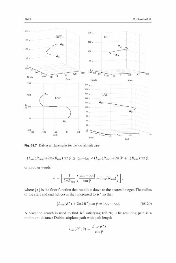
The parameters required to define a low-altitude Dubins airplane path are the sameparameters for the Dubins car given in (68.18) with the addition of the optimalflight-path angle !" and the angles of the start and end helices s and e . Note thatfor the Dubins car path s and e are not required since the orbit is flat and doesnot have a starting location. However, as described in Sect. 68.3.3, to follow a helix,the start angle is required. Figure 68.7 shows several Dubins airplane paths for thelow-altitude case where the altitude difference is 25 m over a typical Dubins car pathlength of 180 m.

68.4.2.2 High-Altitude Dubins PathsIn the high-altitude case, the altitude gain cannot be achieved by flying the Dubinscar path within the flight-path angle constraints. As shown in Chitsaz and LaValle(2007), the minimum-distance path is achieved when the flight-path angle is setat its limit of ˙ N! , and the Dubins car path is extended to facilitate the altitudegain. While there are many different ways to extend the Dubins car path, thischapter extends the path by spiraling a certain number of turns at the beginningor end of the path and then by increasing the turn radius by the appropriateamount.

For UAV scenarios, the most judicious strategy is typically to spend most of thetrajectory at as high an altitude as possible. Therefore, if the altitude at the endconfiguration is higher than the altitude at the start configuration, then the path willbe extended by a climbing helix at the beginning of the path, as shown in the RSRand RSL cases in Fig.68.8. If on the other hand, the altitude at the start configurationis higher than the end configuration, then the path will be extended by a descendinghelix at the end of the path, as shown in the LSR and LSL cases in Fig. 68.8. Ifmultiple turns around the helix are required, then the turns could be split betweenthe start and end helices and still result in the same path length. For high-altitudeDubins paths, the required number of turns in the helix will be the smallest integerk such that

1692 M. Owen et al.

Fig. 68.7 Dubins airplane paths for the low-altitude case

.Lcar.Rmin/C2&kRmin/ tan N! " jzde!zds j<.Lcar.Rmin/C2&.k C 1/Rmin/ tan N! ;

or in other words

k D*

1

2&Rmin

( jzde ! zds jtan N! !Lcar.Rmin/

)+;

where bxc is the floor function that rounds x down to the nearest integer. The radiusof the start and end helices is then increased to R" so that

&Lcar.R

"/C 2&kR"'tan N! D jzde ! zds j: (68.20)

A bisection search is used to find R" satisfying (68.20). The resulting path is aminimum-distance Dubins airplane path with path length

Lair.R"; N!/ D Lcar.R

"/cos N! :

68 Implementing Dubins Airplane Paths on Fixed-Wing UAVs 1693

Fig. 68.8 Dubins airplane paths for the high-altitude case

The parameters required to define a high-altitude Dubins airplane path are the sameparameters for the Dubins car given in (68.18) with Rmin replaced by R", theaddition of the optimal flight-path angle ˙ N! , the additions of the start and end angles s and e , and the addition of the required number of turns at the start helix ks andthe required number of turns at the end helix ke . Figure 68.8 shows several Dubinsairplane paths for the high-altitude case where the altitude difference is 300 m overa typical Dubins car path length of 180 m.

68.4.2.3 Medium-Altitude Dubins PathsIn the medium-altitude case, the altitude difference between the start and endconfigurations is too large to obtain by flying the Dubins car path at the flight-path

1694 M. Owen et al.

zs

cs

ce

ci

ze

zi

ϕ

Fig. 68.9 The start positionof the intermediate arc isfound by varying '

angle constraint, but small enough that adding a full turn on the helix at thebeginning or end of the path and flying so that ! D ˙ N! results in more altitudegain than is needed. As shown in Chitsaz and LaValle (2007), the minimum-distancepath is achieved by setting ! D sign .zde ! zds/ N! and inserting an extra maneuverin the Dubins car path that extends the path length so that the altitude gain when! D ˙ N! is exactly zde ! zds . While there are numerous possible ways to extend thepath length, the method proposed in this chapter is to add an additional intermediatearc to the start or end of the path, as shown in Fig. 68.9. If the start altitude is lowerthan the end altitude, then the intermediate arc is inserted immediately after thestart helix, as shown for cases RLSR and RLSL in Fig. 68.11. If on the other hand,the start altitude is higher than the end altitude, then the intermediate arc is insertedimmediately before the end helix, as shown for cases LSLR and LSRL in Fig.68.11.

To find the Dubins path in the medium-altitude case, the position of theintermediate arc is parameterized by ' as shown in Fig. 68.9, where

zi D cs CR.'/.zs ! cs/:

A standard Dubins car path is planned from configuration .zi ; s C '/ to the endconfiguration, and the new path length is given by

L.'/ D 'Rmin C Lcar.zi ; s C '; ze; e/:

68 Implementing Dubins Airplane Paths on Fixed-Wing UAVs 1695

zs

ws

wℓ

qℓ

qe

qs

Hs

He

ze = we

cs

ce

Hiqi

ci

λs = −1

λi = 1

wi

Hℓ

ψe

λe = 1

ψs

ψi

Fig. 68.10 Parameters thatdefine Dubins airplane pathwhen an intermediate arc isinserted

A bisection search algorithm is used to find the angle '" so that

L.'"/ tan N! D jzde ! zds j:

The length of the corresponding Dubins airplane path is given by

Lair D L.'"/cos N! :

The parameters needed to describe the Dubins airplane path for the medium-altitude case are shown in Fig. 68.10. The introduction of an intermediate arcrequires the additional parameters ci , i , %i , wi , and qi . Therefore, in analogyto (68.18), the parameters that define a Dubins airplane path are

Dair D .R; !; cs; s;%s;ws;qs ; ci ; i ;%i ;wi ;qi ;w`;q`; ce; e;%e;we;qe/:(68.21)

Figure 68.11 shows several Dubins airplane paths for the medium-altitude casewhere the altitude difference is 100 m over a typical Dubins car path lengthof 180 m.

1696 M. Owen et al.

Fig. 68.11 Dubins airplane paths for the medium-altitude case

68.4.3 Path Manager for Dubins Airplane

The path manager for the Dubins airplane is shown in Fig. 68.12. With referenceto (68.14), the start helix is defined as Phelix.cs; s;%s; R; !/. Similarly, theintermediate arc, if it exists, is defined by Phelix.ci ; i ;%i ; R; !/, and the end helixis given by Phelix.ce; e;%e; R; !/. With reference to (68.9), the straight-line path isgiven by Pline.w`;q`/.

68.4.4 Simulation Results

This section provides some simulation results where Dubins airplane paths areflown on a full six-degree-of-freedom UAV simulator. The aircraft used for the

68 Implementing Dubins Airplane Paths on Fixed-Wing UAVs 1697

Follow start helix

Intermediate arc at

beginning Follow intermediate arc

yes

Follow straight line

no

Intermediate arc at end Follow intermediate arc

yes

Follow end helix

no

Cross Hs

Cross Hi

Cross He

Cross Hℓ

Cross Hi

END

Fig. 68.12 Flow chart for the path manager for following a Dubins airplane path

simulation is the Aerosonde model described in Beard and McLain (2012). A low-level autopilot is implemented to regulate the commanded airspeed, bank angle, andflight-path angle. The windspeed in the simulation is set to zero. The simulation isimplemented in Matlab/Simulink.

The simulation results for a low altitude gain maneuver are shown in Fig. 68.13,where the planned trajectory is shown in green and the actual trajectory is shown inblack. The difference between the actual and planned trajectories is due to fact thatthe actual dynamics are much more complicated than the kinematic model givenin (68.1). Simulation results for a medium altitude gain maneuver are shown inFig. 68.14, and simulation results for a high altitude gain maneuver are shown inFig. 68.15.

68.5 Conclusion

This chapter describes how to plan and implement Dubins airplane paths for smallfixed-wing UAVs. In particular, the Dubins airplane model has been refined tobe more consistent with standard aeronautics notation. A complete architecturefor following Dubins airplane paths has been defined and implemented and isshown in Fig. 68.1. Dubins airplane paths consist of switching between helical and

1698 M. Owen et al.

050

100150

200

050

100150

200

0

50

100

150

200

250

NorthEast

Alti

tude

planned

actual

Fig. 68.13 Simulation results for Dubins path with low altitude gain

050

100150

200

050

100150

200

0

50

100

150

200

250

NorthEast

Alti

tude

plannedactual

Fig. 68.14 Simulation results for Dubins path with medium altitude gain

straight-line paths. The vector-field method described in Goncalves et al. (2010)has been used to develop guidance laws that regulate the Dubins airplane to followthe associated helical and straight-line paths. For medium and high altitude gainscenarios, there are many possible Dubins paths. This chapter suggests selecting thepath that maximizes the average altitude of the aircraft during the maneuver.

There are many possible extensions that warrant future work. First, there is aneed to extend these methods to windy environments, including both constant windand heavy gusts. Second, the assumed fast inner loops on airspeed, roll angle, andflight-path angle are often violated, especially for flight-path angle. There may be

68 Implementing Dubins Airplane Paths on Fixed-Wing UAVs 1699

050

100150

200

050

100150

200

0

50

100

150

200

250

NorthEast

Alti

tude

planned

actual

Fig. 68.15 Simulation results for Dubins path with high altitude gain

some advantage, for path optimality in particular, to factoring the time constantsof the inner loops into the planning procedure. Third, this chapter assumes adecoupling between flight-path angle and airspeed. Except for highly overpoweredvehicles, however, achieving a positive flight-path angle will reduce the airspeed,and achieving a negative flight-path angle will increase the airspeed. Taking theseeffects into account will obviously change the optimality of the paths. Finally,there are a variety of methods that have been proposed for achieving vector-fieldfollowing (see Lawrence et al. 2008; Park et al. 2007; Nelson et al. 2007). Themethod used in this chapter is only one possibility, that, in fact, proved challengingto tune. One of the issues is that the method assumes single integrator dynamicsin each direction of motion. More robust 3D vector-field following techniques thataccount for the nonholonomic kinematic model of the Dubins airplane need to bedeveloped.

References

R. Anderson, D. Milutinovic, A stochastic approach to Dubins feedback control for target tracking.In Proceedings of the IEEE/RSJ International Conference on Intelligent Robots and Systems,San Francisco, Sept 2011

A. Balluchi, A. Bicchi, A. Balestrino, G. Casalino, Path tracking control for Dubins cars, inProceedings of the International Conference on Robotics and Automation, Minneapolis, 1996,pp. 3123–3128

R.W. Beard, T.W. McLain, Small Unmanned Aircraft: Theory and Practice (Princeton UniversityPress, Princeton, 2012)

S. Brunke, M.E. Campbell, Square root sigma point filtering for real-time, nonlinear estimation.J. Guid. 27(2), 314–317 (2004)

H. Chitsaz, S.M. LaValle, Time-optimal paths for a Dubins airplane, in Proceedings of the 46thIEEE Conference on Decision and Control, New Orleans, Dec 2007, pp. 2379–2384

1700 M. Owen et al.

R.V. Cowlagi, P. Tsiotras, Shortest distance problems in graphs using history-dependent transitioncosts with application to kinodynamic path planning, in Proceedings of the American ControlConference, St. Louis, June 2009, pp. 414–419

L.E. Dubins, On curves of minimal length with a constraint on average curvature, and withprescribed initial and terminal positions and tangents. Am. J. Math. 79, 497–516 (1957)

J. Egbert, R.W. Beard, Low-altitude road following using strap-down cameras on miniature airvehicles. Mechatronics 21(5), 831–843 (2011)

J. Elston, E.W. Frew, Hierarchical distributed control for search and track by heterogeneous aerialrobot network, in Proceedings of the International Conference on Robotics and Automation,Pasadena, May 2008, pp. 170–175

J. Elston, B. Argrow, A. Houston, E. Frew, Design and validation of a system for targetedobservations of tornadic supercells using unmanned aircraft, in Proceedings of the IEEE/RSJInternational Conference on Intelligent Robots and System, Taipei, Oct 2010, pp. 101–106E

E. Frew, T. McGee, Z. Kim, X. Xiao, S. Jackson, M. Morimoto, S. Rathinam, J. Padial,R. Sengupta, Vision-based road-following using a small autonomous aircraft, in 2004 IEEEAerospace Conference Proceedings, Big Sky, Mar 2004, vol. 5, pp. 3006–3015

E.W. Frew, C. Dixon, J. Elston, M. Stachura, Active sensing by unmanned aircraft systems inrealistic communications environments, in Proceedings of the IFAC Workshop on NetworkedRobotics, Golden, Oct 2009

V.M. Goncalves, L.C.A. Pimenta, C.A. Maia, B.C.O. Durtra, G.A.S. Pereira, Vector fields for robotnavigation along time-varying curves in n-dimensions. IEEE Trans. Robot. 26(4), 647–659(2010)

C. Hanson, J. Richardson, A. Girard, Path planning of a Dubins vehicle for sequential targetobservation with ranged sensors, in Proceedings of the American Control Conference, SanFrancisco, June 2011, pp. 1698–1703

S. Hosak, D. Ghose, Optimal geometrical path in 3D with curvature constraint, in Proceedingsof the IEEE/RSJ International Conference on Intelligent Robots and Systems (IROS), pages113–118, Taipei, Oct 2010

S. Karaman, E. Frazzoli, Incremental sampling-based algorithms for optimal motion planning. Int.J. Robot. Res. 30(7), 846–894 June 2011

D.A. Lawrence, E.W. Frew, W.J. Pisano, Lyapunov vector fields for autonomous unmanned aircraftflight control. AIAA J. Guid. Control Dyn. 31, 1220–12229 (2008)

F.L. Lewis, Optimal Control (Wiley, New York, 1986)R. Mahony, T. Hamel, J.-M. Pflimlin, Nonlinear complementary filters on special orthogonal

group. IEEE Trans. Autom. Control 53(5), 1203–1218 (2008)E.A. Misawa, J.K. Hedrick, Nonlinear observers – state-of-the-art survey. Trans. ASME J. Dyn.

Syst. Meas. Control 111, 344–352 (1989)R.C. Nelson, Flight Stability and Automatic Control, 2nd edn. (McGraw-Hill, Boston, 1998)D.R. Nelson, D.B. Barber, T.W. McLain, R.W. Beard, Vector field path following for miniature air

vehicles. IEEE Trans. Robot. 37(3), 519–529, (2007)S. Park, J. Deyst, J.P. How, Performance and Lyapunov stability of a nonlinear path-following

guidance method. AIAA J. Guid. Control Dyn. 30(6), 1718–1728 (2007)W.F. Phillips, Mechanics of Flight, 2nd ed. (Wiley, Hoboken, 2010)A. Rahmani, X.C. Ding, M. Egerstedt, Optimal motion primitives for multi-UAV convoy protec-

tion, in Proceedings of the International Conference on Robotics and Automation, Anchorage,May 2010, pp. 4469–4474

S. Rathinam, Z. Kim, A. Soghikian, R. Sengupta, Vision based following of locally linear structureusing an unmanned aerial vehicle, in Proceedings of the 44th IEEE Conference on Decisionand Control and the European Control Conference, Seville, Dec 2005, pp. 6085–6090

T. Shima, S. Rasmussen, D. Gross, Assigning micro UAVs to task tours in an urban terrain. IEEETrans. Control Syst. Technol. 15(4), 601–612 (2007)

S.C. Spry, A.R. Girard, J.K. Hedrick, Convoy protection using multiple unmanned aerial vehicles:organization and coordination, in Proceedings of the American Control Conference, Portland,June 2005, pp. 3524–3529

68 Implementing Dubins Airplane Paths on Fixed-Wing UAVs 1701

B.L. Stevens, F.L. Lewis, Aircraft Control and Simulation, 2nd ed. (Wiley, Hoboken, 2003)P.B. Sujit, J.M. George, R.W. Beard, Multiple UAV coalition formation, in Proceedings of the

American Control Conference, Seattle, June 2007, pp. 2010–2015G. Yang, V. Kapila, Optimal path planning for unmanned air vehicles with kinematic and tactical

constraints, in Proceedings of the IEEE Conference on Decision and Control, Las Vegas, 2002,pp. 1301–1306

T.R. Yechout, S.L. Morris, D.E. Bossert, W.F. Hallgren, Introduction to Aircraft Flight Mechanics.AIAA Education Series (American Institute of Aeronautics and Astronautics, Reston, 2003)

C. Yong, E.J. Barth, Real-time dynamic path planning for Dubins’ nonholonomic robot, inProceedings of the IEEE Conference on Decision and Control, San Diego, Dec 2006,pp. 2418–2423

H. Yu, R.W. Beard, A vision-based collision avoidance technique for micro air vehicles usinglocal-level frame mapping and path planning. Auton. Robots 34(1–2), 93–109 (2013)