Implementing a Reconciliation and Balancing Model in the U.S. Industry Accounts*

Dylan G. Rassier† Thomas F. Howells III

Edward T. Morgan Nicholas R. Empey Conrad E. Roesch

U.S. Department of Commerce Bureau of Economic Analysis

Industry Accounts Washington, DC

September, 2007

* We thank Baoline Chen for contributing motivation and knowledge to this project through her study to reconcile and balance the 1997 industry accounts (Chen, 2006). We also thank Karen Horowitz, Douglas Meade, Mark Planting, and George Smith for providing early direction, leadership, and advice to the project. This paper has been prepared for presentation at the 2007 Federal Committee on Statistical Methodology Research Conference in Crystal City, VA, November 5 – 7, 2007. We thank Baoline Chen, Sumiye Okubo, George Smith, Erich Strassner, Mary Streitwieser, and Bob Yuskavage for helpful comments. All errors and omissions are our own. The views expressed in this paper are solely those of the authors and not necessarily those of the U.S. Bureau of Economic Analysis or the U.S. Department of Commerce. † Corresponding author: Dylan Rassier, U.S. Bureau of Economic Analysis, Industry Accounts (BE-40), 1441 L St. NW, Washington DC 20230; e-mail dylan.rassier@bea.gov; phone 202-606-9575; fax 202-606-5366.

1. Introduction In a series of papers beginning with Stone et al. (1942), Stone (1961, 1968, 1970, 1975, 1976, and 1984) advocates a generalized least squares framework to improve the economic and statistical accuracy of independent estimates of national income and expenditures based on relative reliabilities of underlying data used to construct the estimates. Researchers have subsequently revised the Stone method to facilitate its implementation (Byron, 1978; van der Ploeg, 1982, 1984), but federal agencies responsible for producing national economic accounts have generally not implemented the method. Two reasons for this have been a lack of technology that is typically required to solve the complex systems of equations faced by federal agencies and a lack of information regarding the relative reliabilities of underlying data used to construct national accounting estimates. While some agencies have resolved the latter challenge with subjective measures of relative reliabilities (Mantegazza and Pisani, 2000; Moyer et al., 2004a, 2004b), a lack of adequate technology has until recently continued to prevent the implementation of the Stone method (Nicolardi, 2000; Tuke and Aldin, 2004). In a recent study, Chen (2006) addresses both challenges by building an empirical model based on the Stone method and incorporating statistical measures of relative reliability in the model to reconcile and balance estimates in the 1997 U.S. industry accounts. As part of the U.S. Bureau of Economic Analysis’ (BEA’s) integration initiative (Yuskavage, 2000; Moyer et al., 2004a, 2004b; Lawson et al., 2006), the Industry Accounts Directorate is building an empirical model based on the Stone method and Chen (2006) in order to reconcile the gross operating surplus component of value-added from the 2002 expenditure-based benchmark input-output accounts and the 2002 income-based gross domestic product (GDP)-by-industry accounts.1 In addition to reconciling gross operating surplus, the model provides a tool for balancing the 2002 benchmark use table.2 The objective of the reconciliation is to use information regarding the relative reliabilities of underlying data that are used to estimate intermediate inputs in the benchmark use table and gross operating surplus in the GDP-by-industry accounts in a balanced input-output framework in order to improve intermediate input estimates and gross operating surplus estimates in both products. In the benchmark use table, gross operating surplus is derived as a residual between the industry distributions of gross output and intermediate inputs, compensation, and taxes. Intermediate inputs in the benchmark use table are derived from external source data and BEA adjustment methodologies.3 In the GDP-by-industry accounts, gross operating surplus is derived from the industry distributions of the gross domestic income (GDI) components of the national income and product accounts as well as BEA adjustment methodologies. Similar to gross operating surplus in the benchmark use table, intermediate inputs in the GDP-by-industry accounts are derived as a residual between the industry distributions of gross output and value-added. Results from current work will be published in the upcoming 2002 benchmark use table.4 A reconciliation model based on the Stone method has five advantages over past models used by the Industry Accounts Directorate. First, the Stone method yields a model that is transparent. The method is widely researched and familiar to national economic accounting agencies as well as national statistical agencies. In addition, models based on the Stone method are easy to describe to users. Second, the Stone method is built on a firm statistical foundation. In particular, the method uses information on the relative reliabilities of initial underlying data from which estimates are derived to make adjustments to the initial estimates in a balanced accounting framework. Thus, a model based on the Stone method yields a set of fully balanced accounts with adjustments that reflect the reliability of the initial data (Chen, 2006). Third, the least squares framework of the Stone method guarantees that adjustments made to initial estimates are as small as necessary to remove discrepancies between estimates and to satisfy the accounting constraints of the model. In this way, the method 1 Note that the term GDP typically refers to expenditure- or production-based estimates. However, estimates for the GDP-by-industry accounts are derived from the industry distribution of the income-based gross domestic income estimates in the national income and product accounts. Thus, contrary to the typical reference, GDP-by-industry accounts are truly income based. 2 The U.S. benchmark input-output accounts are composed of several tables, including the make table, the use table, and supplementary tables (Lawson et al., 2002). This paper focuses on the benchmark use table, which shows commodities consumed by industries and final users as well as value-added contributed by industries. The benchmark make table has been balanced separately using a different methodology. The supplementary tables are outside the scope of this paper. 3 Likewise, gross output, compensation, and taxes in the benchmark use table are derived from external source data and BEA adjustment methodologies. However, the reconciliation model only adjusts intermediate inputs and gross operating surplus, so this paper focuses only on the external source data and BEA adjustment methodologies used to derive intermediate inputs and gross operating surplus. 4 In contrast, a prior reconciliation based on a different model set a best level for value-added in the 1997 benchmark use table for use in the GDP-by-industry accounts (Moyer et al., 2004a, 2004b).

yields final estimates that are consistent with the economic concepts upon which the accounts are built. Fourth, the Stone method yields a model that is flexible (Chen, 2006). The model can be implemented with aggregated data or disaggregated data. The objective function can be easily altered to include the reliability-weighted squared differences of additional variables. Constraints can be easily removed or imposed. Finally, the Stone method yields a model that is replicable. If no changes are made to data that are introduced to the model, the model yields a duplicate set of results. Alternatively, updated data can be introduced to the model without requiring any substantial changes to the model. This paper presents work by the Industry Accounts Directorate of the BEA to develop and implement an empirical model based on the Stone method and Chen (2006) to reconcile gross operating surplus estimates in the 2002 benchmark input-output accounts and the 2002 GDP-by-industry accounts as well as to balance the benchmark use table. In this spirit, the paper presents the empirical model and briefly describes the technology used to solve the model. Work during development of the model shows that reconciling and balancing a large system with disaggregated data is computationally feasible and efficient in pursuit of an economically accurate and reliable benchmark use table. Section 2 of the paper discusses the benchmark input-output accounts, focusing specifically on the use table, and section 3 discusses the GDP-by-industry accounts. In addition to providing overviews of the accounts, each section discusses features of external source data and BEA adjustment methodologies that are relevant for the reconciliation. Section 4 presents the empirical model as well as a discussion of the construction of reliability measures in the absence of a complete variance-covariance matrix required by theory to obtain an efficient estimator. Section 5 briefly describes the technology used to solve the model, and section 6 presents a set of preliminary results from the model. Section 7 concludes. 2. The U.S. Benchmark Input-Output Accounts The benchmark input-output accounts are prepared quinquennially and provide a comprehensive picture of the flows of goods and services across all consuming industries and final use categories. The accounts are presented in a series of tables. The use table incorporates a complete, balanced set of economic statistics and presents a full accounting of industry and final use transactions. In addition, the use table provides gross output estimates for industries and commodities, value-added estimates by industry, a cross check for the variety of data used to estimate the national income and product accounts, and estimates of final consumption for the national income and product accounts that incorporate the best data available and are in balance with industry inputs and outputs. Chart 1 provides an overview of the structure of the benchmark use table. The matrix in the upper left corner of the use table is the matrix of intermediate inputs, which shows commodities purchased by industries for the production of goods and services in those industries.5 The matrix below the intermediate inputs is the matrix of value-added components, which includes compensation, taxes on imports less subsidies, and gross operating surplus. The matrix to the right of the intermediate inputs is the matrix of final use categories, which includes personal consumption expenditures, private equipment and software, structures, changes in private inventories, government expenditures, exports, and imports. Finally, the bottom row and the far right column show the gross output for industries and commodities, respectively, which come from the balanced benchmark make table. Intermediate input estimates in the benchmark use table are derived using expense data from the Census Bureau, data from non-Census sources, and BEA adjustment methodologies. Approximately 71 percent of the value of intermediate inputs comes from Census expense data, 22 percent of the value comes from non-Census data, and 7 percent of the value comes from BEA adjustment methodologies. Expense data from Census for 2002 are more comprehensive and improved than were available for previous benchmark use tables in the manufacturing sectors (NAICS 31 – 33) and the service sectors (NAICS 42 – 81).6 Within the manufacturing 5 The publication level of detail in the benchmark use table includes approximately 400 industries and 400 commodities. The working level of detail includes approximately 1,000 industries and 1,000 commodities. Commodities are further disaggregated into approximately 9,000 items. Industry analysts estimate transactions for items purchased by industries for the production of goods and services in those industries. The model is implemented with the item level of detail. 6 However, intermediate input estimates continue to be derived entirely or partially from non-Census data and BEA adjustment methodologies for the following sectors: agriculture, forestry, fishing, and hunting (NAICS 11), utilities (NAICS 22), transportation and warehousing (NAICS 48-49), information (NAICS 51), finance and insurance (NAICS 52), real estate (NAICS 53), and education (NAICS 61).

sectors, nineteen categories of expenses are available from the 2002 Economic Census.7 Within the service sectors, nineteen categories of expenses are available from the 2002 Business Expenses Survey (BES).8 Given this depth of coverage in the manufacturing sectors and service sectors, initial gross operating surplus estimates in the benchmark use table are much improved in those sectors both before and after the reconciliation because gross operating surplus is calculated as a residual: industry gross output less intermediate inputs, compensation, and taxes. Expense categories provide a basis for each industry’s input category control estimates in the benchmark data.9 However, adjustments to the input category control estimates similar to adjustments that are made to derive each industry’s estimate of gross output are required in order to maintain equality among industry inputs and outputs. In particular, adjustments are made for non-employer expenses, misreporting and non-filing, and auxiliary services.10 The Economic Census only covers establishments with employees and payroll. Thus, BEA makes an adjustment to capture outputs and inputs for non-employer establishments. Census provides receipts for non-employers derived from administrative data, which are used to estimate the gross output of non-employers.11 For each industry, the ratio of inputs to outputs is assumed to be the same for employers and non-employers. Thus, expenses for non-employers are estimated in a given industry by distributing total receipts for non-employers based on the ratio of inputs to outputs for employers in the industry, with the residual being distributed to gross operating surplus. Given the reasonable underlying assumption and the reliable source data for non-employers, the adjustment for non-employer expenses is considered to be more reliable than other adjustments in the benchmark data but less reliable than data from the Economic Census. Unlike non-employer establishments, small employers are included in estimates published for the Economic Census. However, similar to non-employers, Census derives estimates for small employers from administrative data. Administrative data for non-employers typically include individual income tax returns, and administrative data for small employers typically include individual, partnership, and corporate income tax returns. Given these administrative data, BEA adjusts estimates for non-employers and small employers for misreporting and non-filing.12 A misreport results when a tax return is filed with incomplete or incorrect information. Non-filing results when a business or individual who earns income fails entirely to file a return. An adjustment for misreporting is based on data from two Internal Revenue Service (IRS) programs: the Taxpayer Compliance Measurement Program (TCMP) and the TCMP-Information Return Program (TCMP-IRP).13 The most recent

7 Expense categories from the 2002 Economic Census for manufacturing sectors include the following: (1) accounting, auditing, and bookkeeping, (2) advertising, (3) communications, (4) computer services, (5) contract labor, (6) depreciation, (7) electricity, (8) fuels, (9) legal services, (10) management, consulting, and administrative services, (11) materials consumed, (12) other expenses, (13) payroll and fringe benefits, (14) refuse removal, (15) re-sales, (16) rental of buildings and other structures, (17) rental of machinery and equipment, (18) repairs and maintenance of buildings and/or machinery, and (19) taxes and license fees. 8 Expense categories from the 2002 BES for service sectors include the following: (1) accounting, auditing, and bookkeeping, (2) advertising, (3) communications, (4) contract labor, (5) data processing and other purchased computer services, (6) depreciation and amortization charges, (7) insurance, (8) lease and rental payments, (9) legal services, (10) packaging and containers, (11) printing, (12) management, consulting, and administrative services, (13) materials and supplies not for resale, (14) other expenses, (15) payroll and fringe benefits, (16) repair and maintenance, (17) taxes and license fees, (18) transportation, shipping, and warehouse services, and (19) utilities. In addition to payroll from the 2002 BES, payroll is available from the 2002 Economic Census, which is considered more reliable than the 2002 BES. Thus, the benchmark data include payroll from the 2002 Economic Census. 9 Input category control estimates are used to guide transactions for industries’ purchases of items for intermediate uses. 10 While other adjustments are made to source data for intermediate inputs, these three adjustments capture the majority of the dollar value of adjustments made in the benchmark data. 11 Census provides receipts for non-employers at a more aggregated level than receipts for employer establishments. To distribute receipts for non-employers to the appropriate industry level, BEA uses a ratio of receipts for small-employer establishments by industry to total receipts for all small employers from the Economic Census. However, these adjustments do not affect the data for the reconciliation because gross output is fixed in the reconciliation model. 12 According to Internal Revenue Service compliance studies, three components contribute to a tax gap between the amount taxpayers should pay and the amount taxpayers actually pay in a timely manner: non-filed returns, underreported income, and underpaid taxes (Brown and Mazur, 2003). 13 Discontinued in the early 1990s, the TCMP was an audit program designed to study compliance patterns and levels of misreporting among sole proprietors from a stratified random sample of individual tax returns. The TCMP-IRP was designed

year for which data are available from a TCMP study is 1988. An adjustment for non-filers is based on data from an exact-match study conducted by Census.14 The most recent year for which data are available from an exact-match study at the time the 2002 benchmark use table is being composed and the 2002 GDP-by-industry accounts were published was 1996. In addition, data from the TCMP, TCMP-IRP, and exact-match studies are provided at a more aggregated level than the industry level in the benchmark use table. Given the infrequencies with which the TCMP, TCMP-IRP, and exact-match studies are conducted and the need to approximate the industry distribution of the adjustments, adjustments based on data from the studies are considered less reliable than other adjustments. BEA makes an adjustment for auxiliary services in order to allocate sector-level expense data to industries served by an auxiliary.15 For a given auxiliary, Census provides expense data tabulated for the sector served by the auxiliary. For each industry, the ratio of industry-level payroll to sector-level payroll is assumed to be the same as industry-level expense to sector-level expense. The adjustment draws upon this assumption and industry-level payroll data to allocate the sector-level expense data to industries served. Additions to intermediate inputs in a given industry served are offset by reductions to gross operating surplus in that industry. The adjustment for auxiliary services is considered more reliable than the misreporting and non-filing adjustment but less reliable than the adjustment for non-employer expenses because of the source data and the relatively strong assumption regarding payroll and other expenses. Before gross operating surplus in the benchmark use table is reconciled with the GDP-by-industry accounts, all benchmark estimates are finalized and reviewed to ensure the data submitted to the model are as complete as possible and consistent with the economic concepts upon which the benchmark use table is built. In particular, total gross industry output must equal total gross commodity output, controls for intermediate inputs and value-added components must equal industry gross output, and commodity gross output must be as fully allocated as possible to intermediate inputs. Likewise, the commodity distributions of final use categories are reconciled with the national income and product accounts, Census-based compensation and tax estimates are scaled to match total compensation and taxes, respectively, in the national income and product accounts. In addition, estimates for intermediate inputs, trade margins, and transportation costs must be non-negative. Furthermore, input-output coefficients and the ratio of value-added by industry to total GDP are examined for unreasonable changes from those in the 1997 benchmark use table. Finally, the industry distribution of initial residual gross operating surplus estimates from the benchmark data are compared with the industry distribution of gross operating surplus estimates from the GDP-by-industry accounts, and total value-added from the GDP-by-industry accounts is compared to total final uses as reconciled with the national income and product accounts. 3. The U.S. Gross Domestic Product-by-Industry Accounts The GDP-by-industry accounts focus on the industry shares of value-added to total GDP as well as contributions of industries to GDP growth and provide an annual time series of estimates for gross output, intermediate inputs, and value-added by industry (Moyer et al., 2004a). Intermediate inputs in the GDP-by-industry accounts are derived as a residual between the industry estimates of extrapolated gross output and value-added. Gross output in the GDP-by-industry accounts is calculated using annual survey data to extrapolate best-level gross output detail from the make table in the most recent benchmark input-output accounts. Best-level estimates of the compensation and tax components of value-added in the GDP-by-industry accounts are derived from the GDI components of the national income and product accounts, and these best-level estimates are used directly. Gross operating surplus in the GDP-by-industry accounts is derived by extrapolating best-level estimates of gross operating surplus from the most recent benchmark use table using the sum of annual GDI-based components of gross operating surplus as an indicator.16 In addition to being utilized as annual indicators, the GDI-based estimates of gross to compare the results of the TCMP audits to information returns (e.g., W-2, 1099-INT, etc.) filed with the IRS in order to capture misreporting that TCMP auditors failed to find. 14 An exact-match study compares records from the Current Population Survey (CPS) to records from the IRS in order to identify and estimate non-filed income for individuals who report income in the CPS but do not file a return with the IRS. 15 An auxiliary is an establishment that provides to other establishments services that may not be part of the economic activities of which the serviced establishment is primarily engaged. 16 Best-level estimates of gross operating surplus from the most recent benchmark use table are derived from a prior reconciliation to set best-level value-added (Moyer et al., 2004a, 2004b). In particular, value-added in the GDP-by-industry accounts was built from GDI components and BEA adjustment methodologies and reconciled with value-added from the 1997 benchmark use table. The resulting best-level value-added includes best-level estimates of compensation, taxes, and gross operating surplus, which are extrapolated in the GDP-by-industry accounts. In order to fit the sum of best-level estimates of compensation, taxes, and gross operating surplus with best-level value-added, estimates of gross operating

operating surplus are used as inputs for the reconciliation model. Thus, estimates of 2002 gross operating surplus used in the reconciliation model are different from estimates of gross operating surplus published in the 2002 GDP-by-industry accounts. GDI-based estimates of gross operating surplus for private, non-farm industries are derived using data from the IRS’s Statistics of Income Division (SOI), data from non-SOI sources, and BEA adjustment methodologies.17 Approximately 47 percent of private, non-farm industries’ gross operating surplus comes from the SOI data, 14 percent comes from the misreporting and non-filing adjustment, 22 percent comes from concept and coverage adjustments, and 17 percent comes from non-SOI data and related adjustments.18 In addition, the SOI data are collected and classified on a company basis. BEA makes an adjustment to convert these company-based data to an establishment basis, which is the production unit used for both the benchmark input-output accounts and the GDP-by-industry accounts. This adjustment shifts gross operating surplus from one industry to another with no impact on total gross operating surplus. Company-based and establishment-based industry estimates differ by an absolute average of 7.7 percent. Similar to the benchmark input-output accounts, BEA also makes a misreporting and non-filing adjustment for non-corporate business income tax-based source data in the GDP-by-industry accounts based on data from the TCMP, TCMP-IRP, and exact-match studies. Thus, the misreporting and non-filing adjustment is considered less reliable than other adjustments. The same assessment regarding the relative reliability of the adjustment is made in both the benchmark data and the GDP-by-industry data. Concept adjustments are a collection of adjustments designed to convert tax accounting-based concepts in the SOI data to economic accounting-based concepts consistent with national accounts. Concept adjustments include the removal of capital gains and dividends from business income. Coverage adjustments are designed to include the activities of entities that contribute to gross domestic product but are not required to file a return with the IRS. Coverage adjustments include adding income earned by Federal Reserve banks and imputing net income for owner-occupied housing. While concept and coverage adjustments are considered more reliable overall than the misreporting and non-filing adjustment, reliability varies by specific adjustment. Adjustments based on administrative data are considered second in reliability only to Economic Census data, and adjustments based on survey data are considered third in reliability of this type of adjustment. The company-establishment adjustment is limited to three of the income components of gross operating surplus derived from corporate income tax data: corporate profits before tax, corporate capital consumption allowance, and corporate net interest. The adjustment is made using a matrix of employment data from Census that relates employment by industry on a company basis and employment by industry on an establishment basis. By assuming that profits before tax, capital consumption allowance, and net interest are the same per employee for all establishments performing the same activity, regardless of the company to which that establishment belongs, the matrix converts the industry distribution of each income component from a company basis to an establishment basis. An employment matrix based on Economic Census data is used to adjust the corporate income tax data available for the reconciliation. Due to the weakness of the assumptions that underlie this adjustment methodology, the company-establishment adjustment is considered less reliable than most concept and coverage adjustments but more reliable than the misreporting and non-filing adjustment. Similar to the benchmark estimates, gross operating surplus estimates from the GDP-by-industry accounts are reviewed and finalized before they are submitted to the reconciliation model. In particular, gross operating surplus levels and the ratio of value-added by industry to total GDP is compared with corresponding measures in the benchmark use table. In addition, the initial GDI-based gross operating surplus estimates are reviewed for reasonability within the context of an annual time series. surplus were adjusted as necessary. Thus, best-level estimates of gross operating surplus from the most recent benchmark use table are a residual determined from best-level estimates of compensation, taxes, and value-added. Gross operating surplus is composed of the following components: corporate profits before tax, corporate capital consumption allowance, corporate net interest, corporate inventory valuation adjustment, business transfer payments, proprietors’ income, non-corporate capital consumption allowance, non-corporate net interest, proprietors’ inventory valuation adjustment, rent and royalties, rental income of persons, and surpluses of government enterprises. 17 Gross operating surplus estimates for farm and general government industries and the owner-occupied housing portion of gross operating surplus estimates in the real estate industry are not reconciled using the model presented in this paper. Thus, a detailed discussion of the data and methodologies used to prepare estimates for these industries is outside the scope of this paper. 18 NIPA tables 7.13, 7.14, 7.16, and 7.17 provide additional detail on the relationship between income components as reported by the IRS and as published by BEA.

4. Reconciling Gross Operating Surplus in a Balanced Input-Output Framework The objective is to reconcile in a balanced input-output framework the expenditure-based residual gross operating surplus estimates by industry in the 2002 benchmark use table with the gross operating surplus estimates derived from income-based external source data and BEA adjustment methodologies in the 2002 GDP-by-industry accounts. Based on an adaptation of Chen (2006), the objective is satisfied with a constrained optimization model that minimizes the reliability-weighted sum of squared differences between initial and final estimates subject to a system of accounting constraints.19 4.1. Empirical Model Estimates of expenditure-based final use categories in the benchmark use table are considered highly reliable and are not allowed to adjust.20 In addition, industry gross output, commodity gross output, and the compensation and tax components of value-added, all in the benchmark use table and all derived from the 2002 Economic Census, are considered to be highly reliable and are not allowed to adjust.21 Thus, the objective function in the model is constructed to adjust intermediate input estimates from the benchmark data and gross operating surplus estimates from the GDP-by-industry data. In addition to identifying fixed elements of the benchmark use table, the system of constraints incorporates the accounting identities upon which the table is built.22 In this way, the model provides a tool for balancing the benchmark use table in addition to improving intermediate input estimates and gross operating surplus estimates in the table. More formally, let z and v denote intermediate inputs and value-added, respectively. Let wz and wv denote variance measures for initial estimates of intermediate inputs and value-added, respectively. Let x, y, YE, and YI denote gross output, final uses, aggregate expenditure-based GDP, and aggregate income-based GDI, respectively. Subscript i indexes industries, k indexes commodities, d indexes final use categories (including imports and exports), and h indexes the components of value-added (i.e., compensation, taxes, and gross operating surplus).23 Superscript 0 denotes an initial value. The model is described mathematically as follows:

Min S {z, v} = ∑∑∑∑−

+−

i hv

hi

hihi

i kzki

kiki

w

vv

w

zz2

,

0,,

2

,

0,, )()(

(4.1.1)

19 Chen (2006) builds an empirical model based on the Stone method and incorporates statistical measures of relative reliability in the model to reconcile and balance estimates in the 1997 U.S. Industry Accounts. While Chen’s (2006) model adjusts gross output, intermediate inputs, and all components of value-added, the model being implemented by the Industry Accounts Directorate only allows intermediate inputs and the gross operating surplus component of value-added to adjust. 20 Fixler and Grimm (2005) show that expenditure-based GDP estimates are reliable over time based on the small magnitude of revisions. 21 The compensation and tax components of value-added are scaled to match the totals in the national income and product accounts. 22 In addition to the stated fixed elements of the benchmark use table, gross operating surplus estimates for farm and general government industries and the owner-occupied housing portion of gross operating surplus estimates in the real estate industry are fixed because they are reconciled using a different methodology. 23 The Industry Accounts Directorate maintains multiple indices of industries and commodities. The most aggregated industry index comprises 65 industries, and the most aggregated commodity index comprises 69 commodities. The most disaggregated industry and commodity indices comprise nearly 1,000 industries and commodities, respectively. Each of the most aggregated industries and commodities comprise a mutually exclusive subset of the most disaggregated industries and commodities. Furthermore, commodities are composed of items. The benchmark database contains data for the most disaggregated industries and items. The GDP-by-industry database contains data for the most aggregated industries and no data for commodities. Because the reconciliation and balancing model is implemented with the most disaggregated industry and item data, the model requires separate indices and constraints to identify the most disaggregated industries included in the most aggregated industries. However, this strategy does not affect the specified model. Thus, for simplicity, this exposition focuses on a single index for industries and commodities.

Subject to:

00,, =−∑∑

ddk

ddk yy k∀ (4.1.2)

00 =− ii xx i∀ (4.1.3)

00 =− kk xx k∀ (4.1.4)

00,, =− oncompensatiioncompensatii vv i∀ (4.1.5)

00

,, =− taxesitaxesi vv i∀ (4.1.6)

0,, =−−∑ ∑k h

hikii vzx i∀ (4.1.7)

0,, =−− ∑∑

ddk

iikk yzx k∀ (4.1.8)

0, =−∑∑

i hhi

E vY (4.1.9)

Initial conditions:

0, =−∑∑ E

k ddk Yy (4.1.10)

E

i i kkii Yzx ≠−∑ ∑∑ 0

,0 (4.1.11)

∑∑ ≠−h

hik

kii vzx 0,

0,

0 i∀ (4.1.12)

∑∑ ≠−i

ikd

dkk zyx 0,

0,

0 k∀ (4.1.13)

00,0

, =−∑ Igos

igosi Yv (4.1.14)

∑∑ =k

ki

i xx (4.1.15)

EI YY ≠0, (4.1.16)

Constraints (4.1.2) to (4.1.6) identify fixed values for final use categories, industry gross output, commodity gross output, compensation, and taxes, respectively.24 Equation (4.1.7) constrains the sum of final estimates for intermediate inputs used

24 Industry gross output and commodity gross output in the benchmark use table come from the balanced benchmark make table. Given the constraints in equations (4.1.3) and (4.1.4), the distribution of commodities produced by industries (i.e., the benchmark make table) is not affected by the model.

by an industry and value-added for the industry to equal gross output for the industry. Equation (4.1.8) constrains the sum of final estimates for a commodity used by industries as an intermediate input and sold for final uses to equal gross output for the commodity. Constraint (4.1.9) indicates that final total value-added equals aggregate expenditure-based GDP. The initial condition in equation (4.1.10) indicates that aggregate expenditure-based GDP is set exogenously by the total commodity distribution of final uses determined through the reconciliation with the national income and product accounts. Equation (4.1.11) indicates that total value-added is not initially equal to aggregate expenditure-based GDP. Equation (4.1.12) indicates that the sum of initial estimates for intermediate inputs used by an industry and value-added for the industry do not equal gross output for the industry. Equation (4.1.13) indicates that the sum of initial estimates for a commodity used by industries as an intermediate input and sold for final uses do not equal gross output for the commodity. The condition in equation (4.1.14) indicates that initial estimates of the gross operating surplus component of value-added come from the income-based GDP-by-industry data. Equation (4.1.15) identifies the initial equality between total industry gross output and total commodity gross output in the benchmark use table.25 The initial condition in equation (4.1.16) identifies the statistical discrepancy between aggregate expenditure-based GDP and aggregate income-based GDI.26 4.2. Reliability Weights The optimal estimator requires a variance-covariance matrix to weight the adjustments made to the initial estimates. In practice, the variance-covariance matrix for initial estimates comprising the benchmark use table and the GDP-by-industry accounts is unavailable. However, information regarding the relative reliabilities of initial estimates is used to construct a variance measure for each estimate in the benchmark data and the GDP-by-industry data. In addition, given the lack of information regarding correlations among the initial estimates, covariance measures are assumed to be zero. While this assumption results in an estimator that is less than efficient, the inefficiency is less than may be introduced if the correlations are incorrectly determined (Byron, 1978; Nicolardi, 2000). The noted variance measures are constructed using coefficients of variation, where available or internally-assigned reliability indicators where coefficients of variation are unavailable.27 Recall that estimates in the benchmark use table and GDP-by-industry accounts are derived from two sources of information: 1) external source data and 2) BEA adjustment methodologies. External source data are subject to sampling and non-sampling errors. Coefficients of variation measure sampling errors and are available for source data provided to BEA by SOI and Census.28 BEA adjustment methodologies are designed and implemented to correct non-sampling errors in external source data. However, the adjustments are themselves subject to non-sampling errors. Thus, BEA analysts assign reliability indicators to individual adjustment records based on a rubric required to ensure a consistent application of the reliability indicators across industries and adjustments common to both the benchmark use table and the GDP-by-industry accounts.29 Table 1 contains a summary of the general rubric used by analysts to assign reliability indicators to individual records.30 As shown in Table 1, internally-assigned reliability indicators range from 1 to 5 in one-unit increments, with 1 indicating the 25 Recall that industry gross output and commodity gross output in the benchmark use table come from the balanced benchmark make table. 26 At the most aggregated industry level and commodity level (i.e., 65 industries and 69 commodities), the model contains 4,550 variables to be solved and 135 constraints to be satisfied. At the most disaggregated industry level and item level (i.e., 987 industries and 8,910 items), the model contains 8,795,157 variables to be solved and 9,963 constraints to be satisfied. However, at the most disaggregated level, the intermediate input portion of the benchmark use table is not fully populated. Thus, the number of variables to be solved decreases accordingly. 27 Coefficients of variation are defined as the standard error of an estimate divided by the estimate. 28 In particular, coefficients of variation are available from SOI for all estimates. Because sampling errors apply to surveys and not censuses, coefficients of variation are available from Census for the expense data from the Business Expenses Survey and purchased services from the Annual Survey of Manufactures portion of the Census of Manufactures. Purchased services include the following expense categories: (1) accounting, auditing, and bookkeeping, (2) advertising, (3) communications, (4) computer services, (5) legal services, (6) management, consulting, and administrative services, (7) other expenses, (8) refuse removal, (9) repairs and maintenance of buildings and/or machinery, and (10) taxes and license fees. 29 In addition, using the noted rubric, BEA analysts assign reliability indicators to all detailed estimates in the benchmark data, including those derived from external source data, regardless of the availability of coefficients of variation. 30 In addition to reviewing estimates from the benchmark data and GDP-by-industry data before the data are submitted to the model, internally-assigned reliability indicators are reviewed for consistency of application across industries, type of adjustment, and data set (i.e., benchmark data and GDP-by-industry data) prior to implementing the model.

most reliable estimates (e.g., Census-based estimates), 5 indicating the least reliable estimates (e.g., misreporting adjustments), and intermediate values indicating intermediately reliable estimates (e.g., concept adjustments). In this way, internally-assigned reliability indicators provide an indication of the percentage error or relative reliability of the related estimate, similar to coefficients of variation. Table 2 contains distributions of internally-assigned reliability indicators and coefficients of variation for all industries and ten randomly chosen and sorted industries.31 The figures shown are the percentages of the value of intermediate inputs and gross operating surplus in the benchmark data and the GDP-by-industry data, respectively. No coefficients of variation are available for Census estimates, so there is generally a smaller percentage of benchmark data with coefficients of variation. As shown in Table 2, coefficients of variation are available for approximately 23 percent of the total intermediate input value in the benchmark data and 47 percent of the total gross operating surplus value in the GDP-by-industry data. However, this result does not hold for industries A and I. In addition, internally-assigned reliability indicators of one are assigned only to Census estimates with no adjustments. Thus, there are no GDP-by-industry data with an internally-assigned reliability indicator of one. Internally-assigned reliability indicators of two and three are assigned to almost 50 percent of the total intermediate input value in the benchmark data and 40 percent of the total gross operating surplus value in the GDP-by-industry data. However, this result varies considerable across industries. Finally, internally-assigned reliability indicators of five are assigned to a higher percentage value of gross operating surplus value in the GDP-by-industry data because the misreporting adjustment plays a larger role in those data. This result holds for all industries. Coefficients of variation range from 0 to 1 with a theoretically infinite number of intermediate values.32 In order to use internally-assigned reliability indicators where coefficients of variation are unavailable, a function is applied to internally-assigned reliability indicators to generate an equivalent scale of reliability across all indicators of reliability (i.e., internally-assigned reliability indicators and coefficients of variation). The function maps internally-assigned reliability indicators, denoted θ, according to an exponential parameter, denoted α, as follows:

αθθ ⎟⎠⎞

⎜⎝⎛ −

=4

1)(f . (4.2.1)

If 1=α , internally-assigned reliability indicators are mapped linearly from 0 to 1 in increments of 0.25. If 1>α , internally-assigned reliability indicators are mapped from 0 to 1, assuming that less-reliable estimates are exponentially less reliable than more reliable estimates. If 1<α , internally-assigned reliability indicators are mapped from 0 to 1, assuming that reliability decreases at a diminishing rate.33 In the end, a reliability indicator exists for each individual record and includes a coefficient of variation, where available or an internally-assigned reliability indicator mapped by equation (4.2.1) where a coefficient of variation is unavailable.34 The reliability indicators range from 0 to 1, with 0 indicating the most reliable estimates and 1 indicating the least reliable estimates.35 Upon generating a reliability indicator for each individual record, a variance measure is constructed for each initial estimate by squaring the product of the initial estimate and the related reliability indicator, denoted CV. The following equations summarize the construction of a variance measure, wz or wv, for each initial estimate of intermediate inputs, z0, and value-added, v0, in equation (4.1.1):

20 )( zCVw z ×= (4.2.2)

31 Industries are randomly chosen and sorted in order to disguise the identity of unpublished industry estimates in subsequent figures with results. 32 Coefficients of variation greater than 1 are limited to 1. In the GDP-by-industry data, 1.8% of the coefficients of variation are greater than 1. In the benchmark input-output data, .05% of the coefficients of variation are greater than 1. 33 Evidence has not been generated regarding an appropriate value for α. Thus, given a lack of any evidence to support α ≠ 1, internally-assigned reliability indicators are mapped assuming α = 1. 34 Given the use of fully disaggregated data in the model, this approach yields a variable with either a coefficient of variation or a mapped internally-assigned reliability indicator for each related estimate. 35 This approach assumes that the best estimates with internally-assigned reliability indicators are as good as the best estimates with coefficients of variation, and the worst estimates with internally-assigned reliability indicators are as bad as the worst estimates with coefficients of variation.

and

20 )( vCVwv ×= . (4.2.3) Thus, according to equation (4.1.1), adjustments in the model are weighted by the reciprocal of the variance measure. 5. Technology As noted in the introduction, recent technology makes implementation of the reconciliation and balancing model possible. In particular, the reconciliation model is solved using the CPLEX solver in the Generalized Algebraic Modeling System (GAMS). GAMS is a flexible optimization software package designed to handle large, complex mathematical programming problems. CPLEX is a GAMS solver with solution algorithms for linear, quadratically constrained, and mixed-integer problems. In particular, CPLEX includes simplex and barrier algorithms. The CPLEX solver automatically chooses the optimal combination of algorithms to efficiently solve the particular model specified. Alternatively, GAMS also allows users to adjust tuning parameters in order to set algorithmic options. The reconciliation model is solved with the combination of algorithms chosen by GAMS. 6. Preliminary Results Preliminary results from the reconciliation are shown for ten industries in Table 3. To disguise unpublished estimates, the sample of industries is randomly chosen and sorted. In addition, all estimates have been scaled by the smallest estimate. Given the specifications of the model, the reconciliation results are generally consistent with prior expectations. For industries with relatively small differences between initial benchmark and GDI gross operating surplus estimates (e.g., industries D, F, G, and J), reconciled estimates are generally close to both initial estimates. For industries with relatively large differences between initial benchmark and GDI gross operating surplus estimates (e.g., A, B, C, E, H, and I), the reconciliation favors benchmark estimates in some industries (e.g., industries A, B, C, H, and I) and GDI estimates in other industries (e.g., industry E). This is a result of the relative reliabilities of estimates in those industries as demonstrated by the smaller relative variance in the data favored by the reconciliation.36 For example, initial benchmark and GDI estimates for industry A are 7,156 and 10,172, respectively, and the relative variances of the initial benchmark and GDI estimates are 207 and 3,109, respectively. Reconciled gross operating surplus for industry A is 7,222, which favors the benchmark data and is consistent with the smaller relative variance in the benchmark data. Likewise, initial benchmark and GDI estimates for industry E are 10,259 and 16,124, respectively, and the relative variances of the initial benchmark and GDI estimates are 20,071 and 11,740, respectively. Reconciled gross operating surplus for industry E is 12,634, which favors the GDP-by-industry data and is consistent with the smaller relative variance in the GDP-by-industry data. In some industries (e.g., industries C, F, and J), reconciled estimates lie just outside the range of initial benchmark and GDI estimates. Recall that the initial estimates are adjusted based on relative reliabilities of other estimates in a given industry as well as estimates in other industries. In addition, there is no constraint specified in the model to yield a value between the two initial estimates. Thus, in order for the industry accounting constraints to be satisfied, the reconciled estimates fall outside the range of initial estimates. An important measure of industry performance is calculated as industry value-added as a percentage share of total GDP. Since gross operating surplus is a component of value-added, Table 4 compares this measure before and after the reconciliation and also compares the percentage shares after the reconciliation to the percentage shares from 1997. The percentage shares before and after the reconciliation are similar in most industries (e.g., industries A, B, C, F, G, and J). However, there are some industries in which the percentage shares before and after the reconciliation are not similar (e.g., industries D, E, H, and I). In all industries except industry E, the percentage shares after the reconciliation are similar to the percentage shares from 1997. Because gross operating surplus measures profits, a higher percentage share in industry E reflects higher profits in that industry.

36 A relative variance is calculated as the aggregate variance for an industry divided by the aggregate estimate in that industry.

To evaluate the balanced intermediate input matrix of the benchmark use table, tables 5 and 6 show a comparison of initial and balanced total industry intermediates and initial and balanced total commodity intermediates, respectively. In addition to the percent change from initial to balanced totals, a column is included in each table for the initial under- or over-allocation of gross output calculated as a percent of gross output.37 For both industry intermediates and commodity intermediates, the percent change from initial totals to balanced totals is generally small. This is a result of small initial under- or over-allocations. The largest percent change for both total industry intermediates and total commodity intermediates occurs in industry C, which also has the largest initial under-allocation. The percent change for total industry intermediates is 34.0 percent, while the percent change for total commodity intermediates is 21.6 percent. The initial under-allocations for total industry intermediates and total commodity intermediates in industry C are 13.4 percent and 28.1 percent, respectively. In addition, industry J experiences a relatively large percent change for total industry intermediates of 8.3 percent with an initial under-allocation of 2.9 percent. Finally, industry G also experiences a relatively large percent change for total commodity intermediates of 12.8 percent with an initial under-allocation of 20.5 percent. In Table 5, the percent changes for total industry intermediates are positive for all industries. However, not all industries are under-allocated (e.g., industries B, G, H, and I). This result occurs because the change for gross operating surplus is negative in order to satisfy the constraint that intermediate inputs plus value-added in the industry are equal to gross output. In Table 6, commodity J is the only over-allocated commodity, which is reflected by the negative change in the total. An important measure of industry technology is calculated as a ratio of total industry inputs to total industry output. Since total industry intermediates can change in the model, Table 7 compares input-output coefficients before and after balancing and also compares coefficients after balancing to coefficients from 1997. The coefficients generally increase slightly after balancing (e.g., A, B, C, D, E, F, G, and J), reflecting increases in total industry intermediates for all industries as shown in Table 5. The coefficients for industries H and I do not increase, reflecting the small increases in total industry intermediates for those industries. Likewise, the coefficient for industry C experiences a large increase, reflecting the large increase in total industry intermediates for that industry. Coefficients after balancing are similar to coefficients from 1997 for most industries (e.g., A, C, D, E, G, I, and J) but different for some industries (e.g., B, F, and H). Coefficients increase over time for industries A and J, indicating more inputs are required in 2002 to produce a unit of output in those industries, but decrease for all other industries, indicating fewer inputs are required in 2002 to produce a unit of output in those industries. Given the generally small changes in input-output coefficients before and after balancing, the changes in coefficients from 1997 to 2002 are most likely explained by changes in technology as reflected in the initial estimates of industry intermediate inputs and gross output. 7. Conclusions This paper presents work by the Industry Accounts Directorate of the BEA to develop and implement a model based on a generalized least squares framework in order to reconcile gross operating surplus estimates in the 2002 benchmark input-output accounts use table and the 2002 GDP-by-industry accounts as well as to balance the benchmark use table. Work during development of the model and preliminary results show that the model is computationally feasible and efficient with a set of fully disaggregated data in pursuit of an economically accurate and reliable benchmark use table. Preliminary results are currently being reviewed and are generally as expected. While the benchmark data and the GDP-by-industry data are subject to review before the model is run, there are unexpected results from the model that help identify opportunities for improvements in the data. While the model yields significant technological improvements over past reconciliation and balancing methods, the review process highlights the fact that industry expert intervention during reconciliation and balancing is inevitable. In particular, intervention efforts focus on improvements to the data being introduced to the model. For example, intermediate inputs should be as complete as possible to ensure that under- and over-allocated output are as small as possible before data are introduced to the model.

37 Under- or over-allocation of gross output occurs because complete information regarding the use of intermediate inputs is unavailable. Thus, estimates regarding the use of intermediate inputs either fail to satisfy output or exceed gross output. In particular, under- or over-allocation of industry gross output refers to the amount by which intermediate inputs plus value-added in a given industry fail to satisfy industry gross output or exceed industry gross output, respectively. Likewise, under- or over-allocation of commodity gross output refers to the amount by which intermediate inputs plus final uses for a given commodity fail to satisfy gross output or exceed commodity gross output, respectively.

As work is completed to implement the model, there are three areas to focus in the future. First, the model can be adapted to other industry products, including the make table of the benchmark input-output accounts, the commodity flow table, and the annual input-output accounts. As a second area of focus for future work, there have been challenges encountered during implementation that programming alone cannot overcome. One such challenge has been working with a benchmark database that is configured for other reconciliation and balancing methodologies, which may be largely remedied by future database reconfigurations. Other challenges with the model may always exist, such as calibrating the degree of precision with which a model of this size is capable of reaching a solution. While expert intervention will always be required in balancing input-output tables, this model provides a giant stepping stone to reduce routine interventions while at the same time improving estimate in the tables. Finally, given the important role of reliability indicators in the determination of final estimates, future work will focus on ways to effectively use coefficients of variation and internally-assigned reliability indicators together as well as ways to ensure the consistent application of internally-assigned reliability indicators. As one way to reduce dependence on internally-assigned reliability indicators, coefficients of variation should be collected from source data providers for expenses in industries not covered by Census. In addition, reliability information other than coefficients of variation may be available for some source data. For example, coefficients of variation are generally not available for the Economic Census, but information on imputation rates may provide a useful objective indication of reliability.

References Brown, Robert E. and Mark J. Mazur. 2003. “IRS’s Comprehensive Approach to Compliance Measurement” paper presented at the National Tax Association Spring Symposium. Byron, Ray P. 1978. “The Estimation of Large Social Account Matrices” Journal of the Royal Statistical Society, Series A, 141(3), 359-367. Chen, Baoline. 2006. “A Balanced System of Industry Accounts for the U.S. and Structural Distribution of Statistical Discrepancy” BEA working paper WP2006-8. Fixler, Dennis and Bruce Grimm. 2005. “Reliability of the NIPA Estimates of U.S. Economic Activity” Survey of Current Business, 85(2), 8-19. Lawson, Ann M.; Kurt S. Bersani; Mahnaz Fahim-Nader; and Jiemin Guo. 2002. “Benchmark Input-Output Accounts of the United States, 1997” Survey of Current Business, 82(12),19-43. Lawson, Ann M.; Brian C. Moyer; Sumiye Okubo; and Mark A. Planting. 2006. “Integrating Industry and National Economic Accounts: First Steps and Future Improvements” in A New Architecture for the U.S. National Accounts; edited by Dale W. Jorgenson, J. Steven Landefeld, and William D. Nordhaus; The University of Chicago Press, Chicago. Mantegazza, Susanna and Stefano Pisani. 2000. “Present Practices and Future Developments” paper presented at the 13th International Conference on Input-Output Techniques, University of Macerata, Italy.

Moyer, Brian C.; Mark A. Planting; Mahnaz Fahim-Nader; and Sherlene K. S. Lum. 2004a. “Preview of the Comprehensive Revision of the Annual Industry Accounts: Integrating the Annual Input-Output Accounts and Gross-Domestic-Product-by-Industry Accounts” Survey of Current Business, 84(3), 38-51. Moyer, Brian C.; Mark A. Planting; Paul V. Kern; and Abigail M. Kish. 2004b. “Improved Annual Industry Accounts for 1998-2003: Integrated Annual Input-Output Accounts and Gross-Domestic-Product-by-Industry Accounts” Survey of Current Business, 84(6), 21-57. Nicolardi, Vittorio. 2000. “Balancing Large Accounting Systems: An Application to the 1992 Italian I-O Table” paper presented at the 13th International Conference on Input-Output Techniques, University of Macerata, Italy. Ploeg, Frederick van der. 1982. “Reliability and the Adjustment of Sequences of Large Economic Accounting Matrices” Journal of the Royal Statistical Society, Series A, 145(2), 169-194. Ploeg, Frederick van der. 1984. “Generalized Least Squares Methods for Balancing Large Systems and Tables of National Accounts” Review of Public Data Use, 12(1), 17-33. Stone, Richard. 1961. Input-Output and National Accounts; Organization for European Economic Cooperation, Paris. Stone, Richard. 1968. “Input-Output Projections: Consistent Prices and Quantity Structures” L’Industria, 2, 212-224. Stone, Richard. 1970. Mathematical Models of the Economy and Other Essays; Chapman and Hall, London. Stone, Richard. 1975. “Direct and Indirect Constraints in the Adjustment of Observations” in Nasjonalregnskap, Modeller og Analyse: Essays in Honour of Off Aukrust; Statistisk Sentralbyrå, Oslo. Stone, Richard. 1976. “The Development of Economic Data Systems” in Social Accounting for Development Planning with Special Reference to Sri Lanka; edited by G.Pyatt et al.; Cambridge University Press, Cambridge. Stone, Richard. 1984. “Balancing the National Accounts: The Adjustment of Initial Estimates – A Neglected Stage in Measurement” in Demand, Equilibrium and Trade: Essays in Honor of Ivor F. Pearce; edited by A. Ingham and A.M. Ulph; St. Martin’s Press, New York, 191-212.

Stone, Richard; James E. Meade; and David G. Champernowne. 1942. “The Precision of National Income Estimates” The Review of Economic Studies, 9(2), 111-125. Tuke, Amanda and Vanna Aldin. 2004. “Reviewing the Methods and Approaches of the UK National Accounts” Economic Trends, 47-57. Yuskavage, Robert E. 2000. “Priorities for Industry Accounts at BEA” paper presented at the November 17, meeting of the BEA Advisory Committee.

Chart 1: Overview of the Structure of the Benchmark Use Table

Construction Manufacturing Trade Information Government Other Services

Total Intermediate

Inputs

Personal Consumption Expenditures

Private Equipment and

Software

Changes in Private

Inventories Exports Imports Government GDP

Total Commodity

Output

Construction

Manufacturing

Commodities Trade

Information

Government

Other Services

Total Intermediate Inputs

Compensation

Value-Added Taxes

Gross Operating Surplus

Total Value-Added

Total Industry Output

Industries Final Uses

Table 1: General Rubric for Assigning Reliability Indicators to Underlying Data

Reliability Indicator

Source of Underlying Data

1

• Economic Census data with no adjustments

2

• Economic Census data with adjustments • Survey data with no adjustments • Concept and coverage adjustments based solely on administrative data • Non-employer adjustments

3

• Survey data with adjustments • Trade association data • Concept and coverage adjustments based on survey data • Auxiliary service adjustments

4

• Company-establishment conversion adjustment • Adjustments based on a combination of analyst judgment and external source data

5

• Misreporting adjustments • Adjustments based solely on analyst judgment

Table 2: Distribution of Reliability Indicators in the Benchmark and the GDP-by-Industry Data40

Industry

Data

1

2

3

4

5

CV

Benchmark

13%

24%

20%

17%

3%

23%

All

GDP-by-industry

0%

11%

27%

2%

13%

47%

Benchmark

0%

0%

10%

2%

3%

85%

A

GDP-by-industry

0%

0%

6%

5%

21%

68%

Benchmark

3%

80%

6%

0%

0%

11%

B

GDP-by-industry

0%

11%

8%

7%

15%

59%

Benchmark

80%

1%

18%

1%

0%

0%

C

GDP-by-industry

0%

6%

2%

26%

11%

55%

Benchmark

0%

1%

99%

0%

0%

0%

D

GDP-by-industry

0%

3%

9%

1%

10%

77%

Benchmark

0%

0%

5%

89%

6%

0%

E

GDP-by-industry

0%

1%

1%

1%

33%

64%

Benchmark

0%

85%

5%

0%

0%

10%

F

GDP-by-industry

0%

3%

16%

7%

22%

52%

Benchmark

0%

73%

6%

0%

0%

21%

G

GDP-by-industry

0%

1%

7%

5%

12%

75%

Benchmark

5%

77%

9%

0%

1%

8%

H

GDP-by-industry

0%

11%

1%

9%

4%

75%

Benchmark

0%

11%

3%

4%

0%

82%

I

GDP-by-industry

0%

0%

11%

2%

34%

53%

Benchmark

0%

0%

54%

4%

0%

42%

J

GDP-by-industry

0%

3%

9%

2%

34%

52%

40 Industries are randomly chosen and sorted. The figures shown are the percentages of the value of intermediate inputs and gross operating surplus in the benchmark and GDP-by-industry data, respectively.

Table 3: Comparing Reconciled GOS to Initial Benchmark GOS and Initial GDP-by-Industry GOS41

Industry

Initial Benchmark

GOS

Benchmark Relative

Variance42

Initial

GDP-by-Industry

GOS

GDP-by-Industry Relative

Variance43

Reconciled GOS

Benchmark Percent Change

GDP-by-Industry Percent Change

A

7,156

207

10,172

3,109

7,222

0.9%

- 29.0%

B

3,122

462

1,727

510

2,593

- 16.9%

50.1%

C

1,000

31

1,456

585

978

- 2.2%

- 32.8%

D

14,859

7,951

12,964

1,784

13,848

- 6.8%

6.8%

E

10,259

20,071

16,124

11,740

12,634

23.1%

-21.6%

F

1,166

472

1,187

784

1,148

- 1.5%

- 3.3%

G

1,877

580

1,332

389

1,626

- 13.4%

22.0%

H

13,923

750

6,083

990

9,842

- 29.3%

61.8%

I

16,915

117

11,323

16,758

15,464

- 8.6%

36.6%

J

2,116

204

2,411

2,077

2,095

- 0.9%

- 13.1%

41 Results come from preliminary data. Industries are randomly chosen and sorted, and values are scaled by the smallest value in the sample. 42 The benchmark relative variance is calculated by aggregating the variances for all intermediate input estimates in a given industry and dividing by the aggregate estimate in the industry. 43 The GDP-by-industry relative variance is calculated by aggregating the variances for all gross operating surplus estimates in a given industry and dividing by the aggregate estimate in the industry.

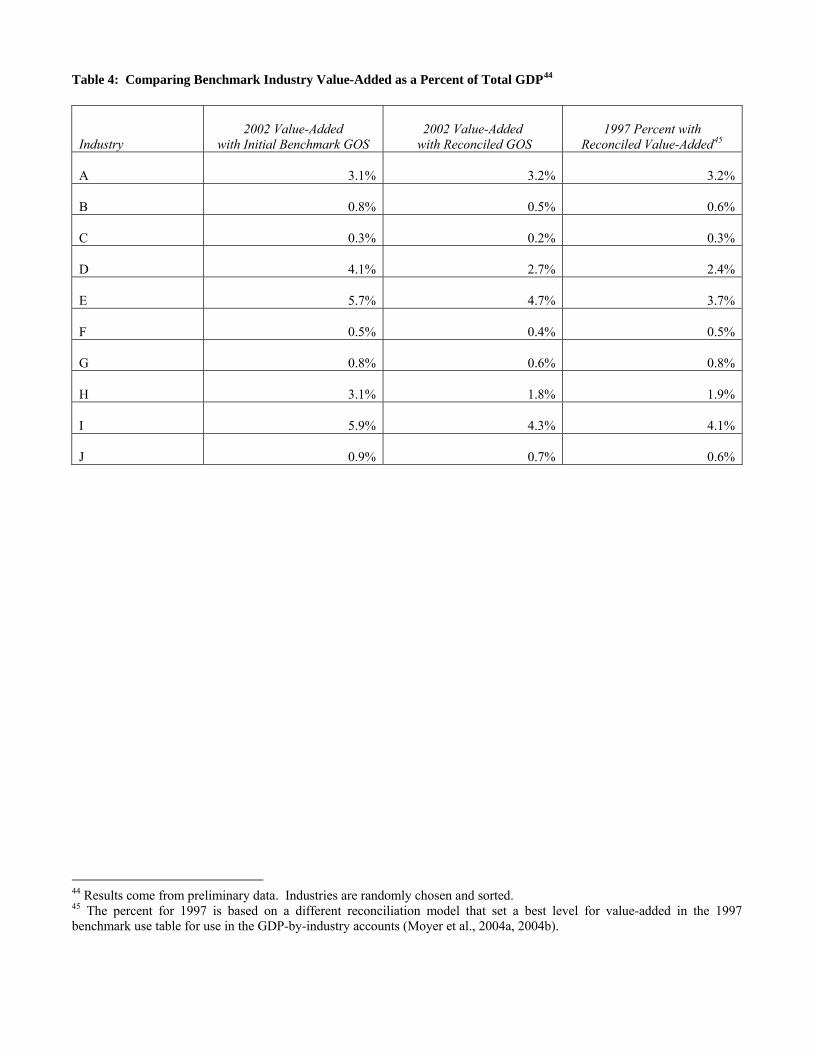
Table 4: Comparing Benchmark Industry Value-Added as a Percent of Total GDP44

Industry

2002 Value-Added

with Initial Benchmark GOS

2002 Value-Added

with Reconciled GOS

1997 Percent with

Reconciled Value-Added45

A

3.1%

3.2%

3.2%

B

0.8%

0.5%

0.6%

C

0.3%

0.2%

0.3%

D

4.1%

2.7%

2.4%

E

5.7%

4.7%

3.7%

F

0.5%

0.4%

0.5%

G

0.8%

0.6%

0.8%

H

3.1%

1.8%

1.9%

I

5.9%

4.3%

4.1%

J

0.9%

0.7%

0.6%

44 Results come from preliminary data. Industries are randomly chosen and sorted. 45 The percent for 1997 is based on a different reconciliation model that set a best level for value-added in the 1997 benchmark use table for use in the GDP-by-industry accounts (Moyer et al., 2004a, 2004b).

Table 5: Comparing Initial and Balanced Industry Intermediates46

Industry

Initial

Intermediate Total

Balanced

Intermediate Total

Percent Change

Initial

Under- or Over-Allocation

A

11,433

11,750

2.8%

1.0%

B

5,142

5,410

5.2%

- 2.0%

C

1,000

1,340

34.0%

13.4%

D

14,567

15,483

6.3%

0.0%

E

25,856

27,303

5.6%

1.3%

F

5,129

5,486

7.0%

4.2%

G

5,871

6,282

7.0%

- 4.8%

H

20,111

20,427

1.6%

- 0.1%

I

14,604

14,617

0.1%

- 0.3%

J

3,090

3,346

8.3%

2.9%

46 Results come from preliminary data. Industries are randomly chosen and sorted, and values are scaled by the smallest value in the sample. The initial under- or over-allocation is calculated as a percentage of industry gross output (i.e., industry gross output less intermediate inputs and value-added divided by industry gross output).

Table 6: Comparing Initial and Balanced Commodity Intermediates47

Commodity

Initial

Intermediate Total

Balanced

Intermediate Total

Percent Change

Initial

Under- or Over- Allocation

A

1,000

1,005

0.5%

0.0%

B

6,433

6,525

1.4%

1.4%

C

1,812

2,203

21.6%

28.1%

D

11,231

11,265

0.3%

0.1%

E

7,033

7,281

3.5%

0.6%

F

7,545

7,743

2.6%

0.8%

G

6,575

7,418

12.8%

20.5%

H

9,267

9,756

5.3%

6.7%

I

35,927

36,465

1.5%

0.0%

J

4,805

4,636

- 3.5%

-1.6%

47 Results come from preliminary data. Commodities are randomly chosen and sorted, and values are scaled by the smallest value in the sample. The initial under- or over-allocation is calculated as a percentage of commodity gross output (i.e., commodity gross output less intermediate inputs and final uses divided by commodity gross output).

Table 7: Comparing Benchmark Input-Output Coefficients with Initial and Balanced Industry Intermediates48

Industry

2002 Input-Output Coefficient

with Initial Intermediates

2002 Input-Output Coefficient with Balanced Intermediates

1997 Input-Output Coefficient with Balanced Intermediates

A

0.33

0.34

0.30

B

0.51

0.54

0.65

C

0.31

0.42

0.50

D

0.42

0.45

0.45

E

0.40

0.42

0.50

F

0.56

0.60

0.71

G

0.52

0.55

0.61

H

0.54

0.54

0.74

I

0.32

0.32

0.34

J

0.38

0.41

0.35

48 Results come from preliminary data. Industries are randomly chosen and sorted.