Implementing 3D Digital SoundIn “Virtual Table Tennis”

By Alexander Stevenson

Introduction

For our term project, Arthur Louie, Adrian Secord, Matthew Brown and I decided to produce a program capable of simulating and playing a virtual game of table tennis.

“Virtual Table Tennis” is the result.

Introduction – What is VTT?

Virtual Table Tennis incorporates physics simulation, AI solving, real-time graphical display, and a flexible input scheme (allowing several different devices, including a Fastrak, to control the paddles).

Virtual Table Tennis allows either a player to face off against the computer, or for the computer to play against itself.

Introduction – VTT in Action

Introduction

This talk however, will ignore all that. Instead we will focus on the topic of digital 3D

positional sound, and how it is implemented in Virtual Table Tennis.

Overview

Our approach How digital sound works How we hear Computing the direction of the sound Results

Our Approach

In deciding on how to produce sound for this project, we had several options.

We decided on a sampled/playback approach to sound, as opposed to a fully simulated approach.

This is because we had a narrow range of sounds to produce, easily captured by samples, and because we wished to devote most compute time to physics/AI.

Our Approach

Further, we were implementing in C/C++ on a Linux platform. This precluded easy integration of some existing Java simulation packages.

It was therefore decided that the best route was a module capable of mixing samples, and modulating them according to the virtual position of the sound they were simulating.

Overview

Our approach How digital sound works How we hear Computing the direction of the sound Results

Digital Sound – Sampling

As with any digital representation of an analog signal, digital sound consists of evenly spaced samples of a sound wave.

Digital Sound – Sampling

The frequency with which we sample determines the range of frequencies we can reproduce. (Nyquist rate)

The number of bits with which we sample determines the dynamic range we can reproduce

Digital Sound - Sampling

Our goal is CD quality sound. This means 44100 Hz, and 16 bit samples.

At this rate, one second of stereo audio requires 2 x 44100 x 2 = 176400 bytes

While this doesn’t seem computationally excessive, we must keep in mind that many sounds may be playing at once, and so our overhead for mixing/playback increases

Digital Sound – Playback

Our program must play sound continuously (2 samples every 2.27e-5 seconds)

But we also need to draw graphics, simulate physics, calculate AI, etc…

Even putting sound in another thread does not let us achieve this.

Digital Sound – Playback

Solution: DMA (Direct Memory Access)– By preloading a buffer with sound information, we

can have the sound card play it back automatically while we process other things (graphics, physics, input, AI, etc.)

– Then, while we are off processing other things, the sound card continues to play sound. When we return from processing, we refill the buffer, and continue.

Digital Sound – Lag vs. Skipping

The response of the system becomes very dependent on the size of the sound buffer.

Large buffers result in a greater buffer against long processing times, but also mean that more data must be played before a new event can be heard.

A size of 4096 bytes produces a lag of 0.022 seconds, which is acceptable for our frame rates. (> 45 fps)

Overview

Our approach How digital sound works How we hear Computing the direction of the sound Results

How We Hear

We have ears! Ideally two of them. This lets us position sounds in space by

comparing the relative volumes we hear in each ear, as well as the timing difference a sound takes to get from one ear to the other.

For an inter-aural distance of 15cm, this time is as much as (0.15m)/(344m/s)=4.36e-4 seconds. This is around 38 (mono) samples!

How We Hear

Of course, how this actually sounds ends up depending on a user’s speaker placement, which is rarely ideal.

Therefore, we’ll ignore the timing differences between ears, and focus solely on the volume differences.

Overview

Our approach How digital sound works How we hear Computing the direction of the sound Results

Computing the sound’s direction

Given a head location, H(x,y,z), a look-at point L(x,y,z), and a sound origin S(x,y,z), we need to figure out where to place the sound in stereo.

Keeping in mind the speakers are in front of us, we would like to put a sound which is 90 degrees to our right, entirely in the right speaker, and 90 degrees to our left in the left speaker.

Computing the Sound’s Direction

First, we will make the simplifying assumption that our head is vertical. That is, that our up vector is (0,0,1).

This means we need only consider angles in the X-Y plane.

Thus H(x,y,z), S(x,y,z), L(x,y,z) become H(x,y), S(x,y), L(x,y).

Computing the Sound’s Direction

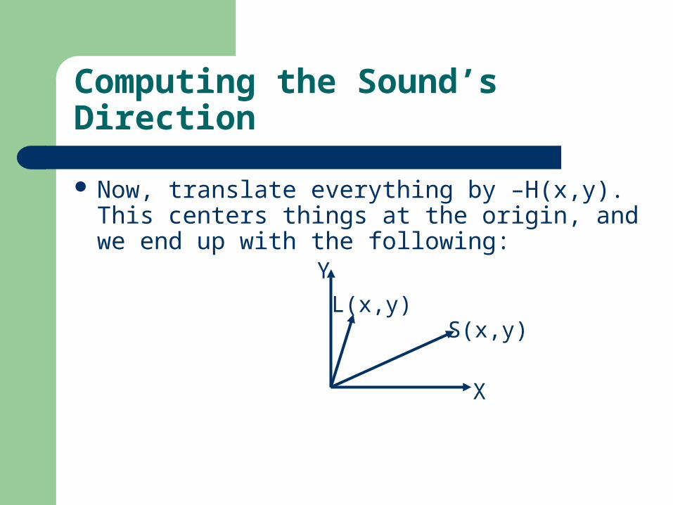
Now, translate everything by –H(x,y). This centers things at the origin, and we end up with the following:

Y

X

L(x,y)S(x,y)

Computing the Sound’s Direction

We now need to determine how far the sound is panned. To do this, we compute the angle between the vector L(x,y) and S(x,y). This narrows the sound down to two locations:

L(x,y)S(x,y)S(x,y)

θθ

Computing the Sound’s Direction

Now, if θ is > 90, then we set θ=180 – θ. This allows us to treat situations where the

sound is in front or behind us the same.

Computing the Sound’s Direction

Finally, to figure out whether the sound is to our left or to our right, we compute the angle between S(x,y) and L(y,-x):

L(x,y)S(x,y)S(x,y)

θ2

θ2

L(y,-x)

If θ2 < 90 then the sound is on our right, otherwise it is on our left.

Computing the Sound’s Direction

Now that we know how many degrees, and to which side, the sound is positioned, we can adjust the panning of the sound appropriately, and mix this sound into our play buffer.

Overview

Our approach How digital sound works How we hear Computing the direction of the sound Results

Results – Features

Virtual Table Tennis has a flexible sound module which supports mixing of multiple streams of digital audio, all with independent stereo positions.

Further, the panning of each sound is dynamically updated as the camera moves, even if the sound is still playing. This is because mixing is done only one buffer at a time.

Results – Features

You can also specify that a sound has no position, allowing things like background music, or referee voices, to simply play center-panned over the speakers.

Results – Performance

Our 3D positional audio mixer performs very well.– It uses only 3 integer operations per sample,

(multiply and shift to set volume, and then an addition to mix the sound into the buffer)

– We can successfully mix > 8 continuous streams on an Athlon 850 MHz CPU.

– It sounds great!

Future Work

Things we have not added are scaling ball collision volume in proportion to the velocity of the impact, and delaying the samples between the speakers to simulate the inter-aural lag.

These might add subtly, but are not critical.

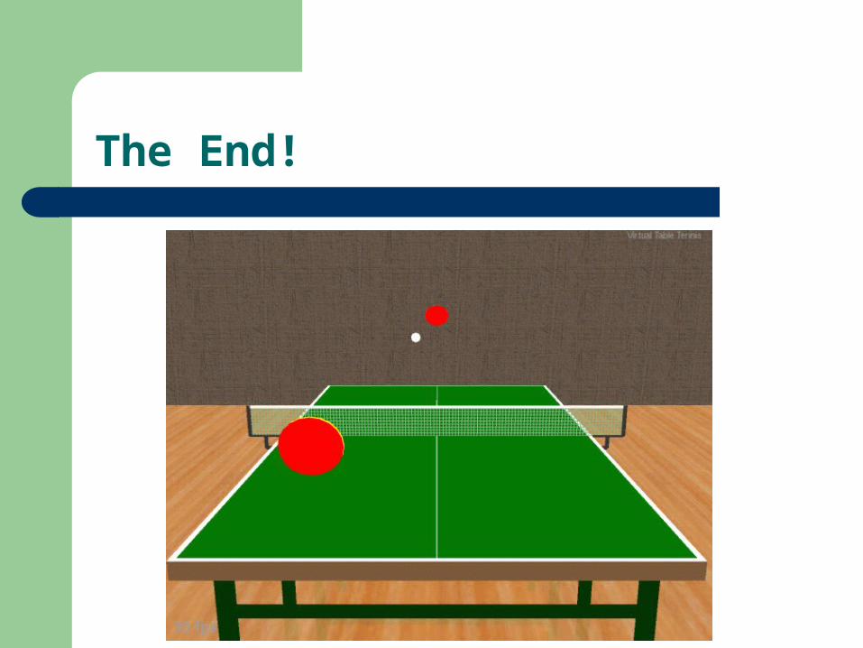
The End!