University of Rhode Island University of Rhode Island

DigitalCommons@URI DigitalCommons@URI

Open Access Master's Theses

2017

Implementation of Moving Magnet Actuation in Very Low Implementation of Moving Magnet Actuation in Very Low

Frequency Acoustic Transduction Frequency Acoustic Transduction

Brenton Wallin University of Rhode Island, brentwallin@my.uri.edu

Follow this and additional works at: https://digitalcommons.uri.edu/theses

Recommended Citation Recommended Citation Wallin, Brenton, "Implementation of Moving Magnet Actuation in Very Low Frequency Acoustic Transduction" (2017). Open Access Master's Theses. Paper 1017. https://digitalcommons.uri.edu/theses/1017

This Thesis is brought to you for free and open access by DigitalCommons@URI. It has been accepted for inclusion in Open Access Master's Theses by an authorized administrator of DigitalCommons@URI. For more information, please contact digitalcommons@etal.uri.edu.

IMPLEMENTATION OF MOVING MAGNET ACTUATION IN VERY LOW

FREQUENCY ACOUSTIC TRANSDUCTION

BY

BRENTON WALLIN

A THESIS SUBMITTED IN PARTIAL FULFILLMENT OF THE

REQUIREMENTS FOR THE DEGREE OF

MASTER OF SCIENCE

IN

OCEAN ENGINEERING

UNIVERSITY OF RHODE ISLAND

2017

MASTER OF SCIENCE THESIS

OF

BRENTON WALLIN

APPROVED:

Thesis Committee:

Major Professor James Miller

Steven Crocker

Gopu Potty

David Taggart

Nasser H. Zawia

DEAN OF THE GRADUATE SCHOOL

UNIVERSITY OF RHODE ISLAND

2017

ABSTRACT

Measuring the performance of hydrophones in submarine and surface ship towed

arrays at low frequencies in the Leesburg test facility (Okahumpka, FL) is achieved using

ambient noise as a calibration source. The preferred method of calibration that relies on a

known, repeatable sound source is not implemented because the equipment capable of

generating sound at such low frequencies does not currently exist.

This project examines the feasibility of implementing a moving magnet actuator

(MMA) as the motor force in a very low frequency (VLF) underwater acoustic projector.

MMAs have the potential to advance low frequency projector technology by providing

large linear displacements and large force outputs in a small package. To explore this

potential, three methods of investigation are performed in this study: analytical modeling,

numerical modeling, and experimental testing. Analytical modeling is performed in Matlab

using fundamental equations for a simple acoustic point source. Numerical modeling is

represented as a fluid-structure interaction (FSI) problem and is solved using the finite

element program Abaqus. Experimental testing is conducted by placing a load on a Bose

MMA to simulate the mass of the VLF projector’s water displacement.

Analytical and numerical modeling efforts estimate a projector source level of over

125 dB// 1 𝜇𝑃𝑎 @1m at 1Hz and over 180 dB// 1 𝜇𝑃𝑎 @1m at 30Hz. The experimental

efforts find that the Bose MMA operates at displacements necessary to achieve sound

pressure levels calculated from the analytical and numerical models. This study indicates

that an MMA is a suitable force generator for the VLF projector and explores future work

necessary for VLF projector design, manufacture, and operation.

iii

ACKNOWLEDGEMENTS

The author wishes to acknowledge the generous individuals who have provided

great support and encouragement to him throughout his thesis project

First, I must acknowledge the Ocean Engineering Department at the University of

Rhode Island. The department has provided me an education for seven years and I am

grateful for the support and efforts from all staff and faculty members who have made this

thesis possible. I would like to extend a special thank you to my major professor, Dr. James

Miller, and co-major professor, Dr. Steven Crocker, for your generous guidance throughout

my master’s thesis project. Your continuous support, thoughtful advice, and willingness to

share your expertise have been invaluable.

I would also like to express my sincere gratitude to many of my peers at the Naval

Undersea Warfare Center. Specifically, I would like to thank Daniel Perez for your

mentorship with finite element modeling, Jeffrey Szelag for your participation in the

experimental testing of the moving magnet actuator, and Dr. Victor Evora and Jay Melillo

for procuring funds to make this project possible.

Lastly, I would like to thank my family and friends who have provided me constant

support. To my mom, dad, and sisters, Courtney and Brittany: as the youngest, I have

always looked up to you. Thank you for being inspiring role models and for instilling a

passion for education in me. To my girlfriend, MacKenzie Rogers, thank you for spending

several days and late nights proofreading this thesis. Your ideas and contributions have

pushed me to excel, and I am forever grateful.

iv

TABLE OF CONTENTS

ABSTRACT ........................................................................................................................ ii

ACKNOWLEDGEMENTS ............................................................................................... iii

TABLE OF CONTENTS ................................................................................................... iv

LIST OF TABLES ............................................................................................................. vi

LIST OF FIGURES .......................................................................................................... vii

CHAPTERS

1 Introduction .......................................................................................................................1

1.1 Motivation ..........................................................................................................1

1.2 Thesis Content ...................................................................................................3

2 Background and Literature Review ..................................................................................5

2.1 Introduction to Acoustics ...................................................................................5

2.2 Introduction to Sonar and Transducers ..............................................................8

2.3 Current Low Frequency Projector Technologies ...............................................9

2.3.1 Moving coil projector .........................................................................9

2.3.2 Bender Bar Transducers ....................................................................11

2.3.3 Hydraulically Actuated Transducers .................................................12

2.4 Moving Magnet Actuation ...............................................................................14

2.4.1 Bose Electroforce Moving Magnet Actuator ....................................15

3 Theoretical Models .........................................................................................................18

3.1 Analytical Method ...........................................................................................18

3.2 Numerical Method ...........................................................................................22

4 Experimental Testing ......................................................................................................37

4.1 Experimental Setup ..........................................................................................37

4.2 Experimental Analysis .....................................................................................39

5 Future work .....................................................................................................................44

v

6 Conclusion ......................................................................................................................46

LIST OF REFERENCES ...................................................................................................48

APPENDIX ........................................................................................................................50

BIBLIOGRAPHY ..............................................................................................................51

vi

LIST OF TABLES

Table 1: Key Specifications of Bose LM3000-25 MMA [10] ...........................................15

Table 2: Material properties for the structure in the numerical model. The

structure refers to the VLF projector. .................................................................32

Table 3: Material properties of the fluid in the numerical model. The fluid refers

to the acoustic domain. .......................................................................................32

Table 4: Tabular data for experimental displacement of MMA radiating face .................42

vii

LIST OF FIGURES

Figure 1: A bathometric map of Bugg Spring, an open water acoustic test facility

located in the Okahumpka, Florida. Bugg Spring is also referred to the

Leesburg test facility or LEFAC. (Image source: [2]) ..........................................1

Figure 2: The ambient noise spectrum observed at the Bugg Spring test facility by

a digital hydrophone line array on May 21, 2012. The weather was clear

and calm. (Image source: [2]) ...............................................................................2

Figure 3: A visualization of transverse (top) and compression (bottom) waves. In

transverse waves, the displacement of material is perpendicular to the

wave’s direction of travel. In compression waves, the displacement of

material is parallel to the wave’s direction of travel. (Image Source: [4]) ...........5

Figure 4: An illustration of pressure waves. During a pressure wave, molecules of

a fluid are displaced causing fluctuations about an equilibrium pressure.

(Image source: [3]) ................................................................................................6

Figure 5: A simple electrodynamic loudspeaker and Lorentz force equations. The

equations show that current flowing through the coil (I) interacting with

the magnetic field (B) will result in a force (F) driving the radiating face.

(Image Source: [7]) .............................................................................................10

Figure 6: The USRD J15-3 moving coil projector. (Image source: [8]) ............................11

Figure 7: An illustration of a bender bar projector. Multiple ceramic bars are

arranged in barrel staves around a cylindrical housing. (Image source:

[8]).......................................................................................................................12

Figure 8: The HX-29 bender bar projector. (Image source: USRD acoustic

augmentation support program (AASP)) ............................................................12

Figure 9: A design of a hydraulically actuated transducer. In a hydraulically

actuated transducer, an amplifier at the center of the device drives two

opposing flexural disks. An electrically driven pump provides hydraulic

power and a low-level electrical signal supplies the hydraulic amplifier

with the signal (Image source: [8]) .....................................................................13

Figure 10: The HLF-1D hydraulic transducer. (Image source: USRD AASP) .................13

Figure 11: A simple schematic of a moving magnet actuator. Current flowing

through the stationary coils interacts with the magnetic field to produce a

force causing the magnet to move. (Image Source: [9]) .....................................14

Figure 12: Solid model of Bose LM3000-25 MMA (Image Source: [10]) .......................15

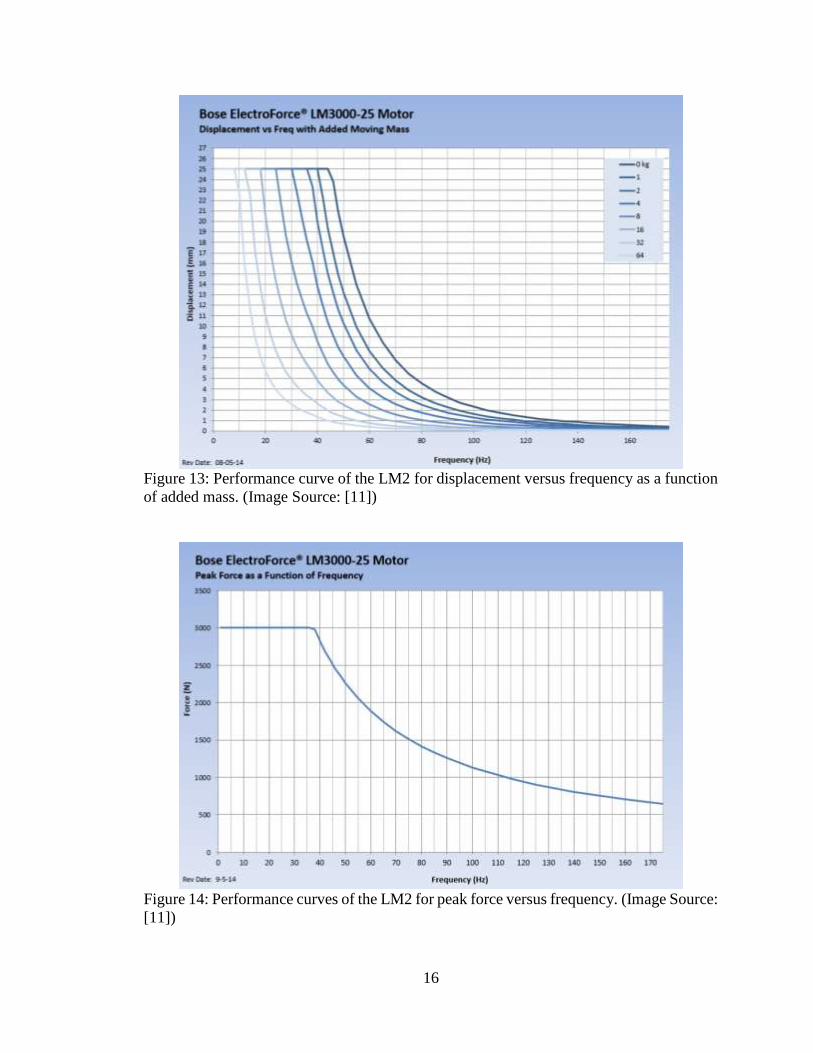
Figure 13: Performance curve of the LM2 for displacement versus frequency as a

function of added mass. (Image Source: [11]) ....................................................16

viii

Figure 14: Performance curves of the LM2 for peak force versus frequency.

(Image Source: [11]) ...........................................................................................16

Figure 15: A design concept for a VLF underwater acoustic projector. The linear

actuator inside the waterproof housing drives a circular piston. A cavity

is designed behind the radiating face for hydrostatic pressure

compensation. .....................................................................................................17

Figure 16: A plot of displacement amplitude for an added mass of 14.1 kg. This

curve was generated using the total mass (piston and radiation mass) and

the Bose performance curves of the LM2 MMA. ...............................................20

Figure 17: A plot of expected source level for the VLF projector using equations

for a simple point source. The shape is defined by a displacement limited

region where the acoustic performance is limited by the peak

displacement of the MMA and the force limited region where the

acoustic performance is limited by the peak force of the MMA. .......................21

Figure 18: A plot of source level for projectors of different size radiating faces.

As the radius of the radiating face increases, source level increases and

the frequency range of the displacement limited region decreases. ....................22

Figure 19: Mesh containing elements with 3 nodes (left) and 4 nodes (right). .................23

Figure 20: SolidWorks model of VLF projector housing and radiating face ....................26

Figure 21: Axisymmetric model of VLF projector (left) and acoustic domain

(right) ..................................................................................................................27

Figure 22: The meshed model of the VLF projector. This structure is meshed with

CAX4R elements and has at least 3 elements through the thinnest parts. ..........29

Figure 23: The meshed acoustic domain. This fluid is meshed with ACAX3

elements and element size grows as it approaches the outer boundary of

the domain. ..........................................................................................................31

Figure 24: Hypermesh model with callouts describing boundary conditions.

Nodes on the fluid structure interface are tied together using a tie

constraint (Abaqus keyword TIE). To simulate an infinite acoustic

domain, a nonreflective boundary is applied to the edge of the acoustic

domain (Abaqus keyword SIMPEDANCE). A point mass node (Abaqus

keyword MASS) is placed at the center of the projector to simulate the

mass of the MMA. To simulate actuator motion, a motor shaft is created

as a connector element between two nodes on the axis of symmetry

(Abaqus Keyword CONN2D2) and a displacement motion (Abaqus

keywords CONNECTOR MOTION) is prescribed to apply a

displacement to the shaft. ....................................................................................33

Figure 25: The plot of the analytical and Abaqus results. .................................................34

ix

Figure 26: Source level plotted for an analytical analysis performed with a

radiating face of radius 0.15m (blue) and 0.175m (black) against the

numerical results. This plot supports the hypothesis that the suspension

geometry could contribute to a higher SL output. ..............................................35

Figure 27: Picture of the experimental test setup. The Bose MMA is mounted to a

massive structure. A test fixture with a spring is used to account for the

effect of gravity of the added mass on the MMA’s radiating face. ....................37

Figure 28: A picture of the equipment to drive the MMA. A signal generator is

used to apply a +/- 10 V command signal to the Bose amplifier that

drives the MMA with a high voltage signal. An oscilloscope is used to

verify the signals being sent to the MMA. ..........................................................38

Figure 29: A picture of the PXI chassis that records the experimental data. Four

channels with recorded on the PI-4462 card: acceleration, command

voltage, voltage across the MMA’s coils, and current applied to the

actuator. ...............................................................................................................39

Figure 30: Plot of the mean values and confidence intervals for experimental

displacement of the MMA. The values are plotted against theoretical

displacement values. ...........................................................................................41

Figure 31: Plot of a regression fit to the experimental data (green). The regression

is a piecewise function that is constant below 18.5 kHz and a decreasing

exponential above 18.5 kHz. The regression fit is plotted against the

theatrical displacements for a 14.1kg added mass based on the Bose

performance curves. ............................................................................................42

1

CHAPTER 1

Introduction

1.1 Motivation

Submarine and surface ship tactical towed array calibration is conducted in

Okahumpka, Florida at Bugg Spring (often referred to as the Leesburg Facility, or LEFAC)

as shown in Figure 1. It is an open water test facility owned and operated by the Naval

Undersea Warfare Center's (NUWC) Underwater Sound Reference Division (USRD).

Geographically isolated and inhabited minimally by aquatic life, the spring is one of the

U.S. Navy's quietest open water facilities. Its funnel shape has a diameter of 130 meters at

the surface and walls that slope at approximately 45 degrees to a maximum depth of 50

meters [1].

Figure 1: A bathometric map of Bugg Spring, an open water acoustic test facility located

in the Okahumpka, Florida. Bugg Spring is also referred to the Leesburg test facility or

LEFAC. (Image source: [2])

2

The low frequency (1-60Hz) performance tests conducted at LEFAC rely on

ambient noise as a calibration signal. A spectrum of the ambient noise can be seen in Figure

2. A limitation of this passive method is the low signal-to-noise ratio of the hydrophones’

outputs; the background electronic noise of the hydrophones may not be much less than

the electronic signal produced by the acoustic noise in the spring [2].

Figure 2: The ambient noise spectrum observed at the Bugg Spring test facility by a digital

hydrophone line array on May 21, 2012. The weather was clear and calm. (Image source:

[2])

USRD would like to replace this passive calibration method with a known source

calibration method. Unfortunately, USRD does not currently have the low frequency

technology in their assortment of transducer standards to perform a known source

calibration down to 1Hz.

With their large linear displacements and force outputs, moving magnet actuators

(MMAs) have the potential to be implemented as the motor force in a very low frequency

3

(VLF) underwater acoustic projector. A VLF projector can be used as the known sound

source for LEFAC’s calibration testing.

The objective of this study is to examine the feasibility of implementing an MMA

as the motor force in a VLF underwater acoustic projector. Modeling of the acoustic output

for the MMA is the first milestone in designing, manufacturing, and implementing a sound

source to replace the ambient noise as the source of the calibration signal.

1.2 Thesis Content

Chapter 2 provides background information critical to the understanding of the

research performed in this study. General knowledge of acoustics and sonar, a review of

the U.S. Navy’s current low frequency projectors, and an introduction to moving magnet

actuation are covered in this chapter.

The research begins in Chapter 3 where two different engineering approaches to

modeling a moving magnet low frequency projector are examined. The first is an analytical

model using fundamental equations for a simple sound source. The second model is a finite

element model using the software package Abaqus.

In addition to the modeling efforts, experimental testing is performed on a Bose

LM2 MMA to validate that it can produce the forces and displacements necessary to

implement the actuator in an underwater projector. The results of this experiment can be

found in Chapter 4.

Although modeling and experimentation of the actuator are performed in this study,

further analyses must still be completed in order to build a device. Chapter 5 discusses

future design work required to build a functioning underwater acoustic projector.

4

Finally, the research concludes in Chapter 6. In this section, the significance of this

study, the methods of analysis and experimentation, and key findings are all summarized.

5

CHAPTER 2

Background and Literature Review

2.1 Introduction to Acoustics

Acoustic waves are vibrational excitations traveling through an elastic medium. As

illustrated in Figure 3, there are two types of acoustic waves: shear waves (top) and

compression waves (bottom). In this visualization, the slinky is the elastic medium. Shear

waves refer to transverse waves where the displacement of material is perpendicular to the

wave’s direction of travel. The coils of the slinky are oscillating up and down, but the

motion of the wave is left to right. Compression (or pressure) waves refer to longitudinal

waves where the displacement of material is parallel to the wave’s direction of travel. These

waves consist of compressions and rarefactions of the medium. In compressions, the

acoustic medium is compressed; there is a temporary state of higher density. Rarefaction

is the opposite; the acoustic medium momentarily decreases in density. The coils of the

springs are oscillating left and right while the motion of the wave is left to right [3].

Figure 3: A visualization of transverse (top) and compression (bottom) waves. In transverse

waves, the displacement of material is perpendicular to the wave’s direction of travel. In

compression waves, the displacement of material is parallel to the wave’s direction of

travel. (Image Source: [4])

6

Because the acoustic medium water is a fluid and fluids lack the shear strength

needed to support transverse waves, only compression waves are considered for the

remainder of the paper. Figure 4 illustrates a pressure wave. When molecules of a fluid are

pushed and pulled apart, they exert a restoring force that opposes the motion. These

periodic pressures fluctuate about an equilibrium pressure also denoted as the hydrostatic

pressure.

Figure 4: An illustration of pressure waves. During a pressure wave, molecules of a fluid

are displaced causing fluctuations about an equilibrium pressure. (Image source: [3])

Mathematically, the one dimensional propagation of these waves are governed by

the second order partial differential equation [5]

𝜕2𝑝

𝜕𝑥2−

1

𝑐2

𝜕2𝑝

𝜕𝑡2= 0

(1)

where 𝑝 is pressure fluctuation from the equilibrium, 𝑥 is position, 𝑡 is time, and 𝑐 is the

speed of sound of the medium. For a sinusoidal pressure wave traveling in one direction,

the solution to Equation 1 is [6]

7

𝑝 = 𝑝0sin (𝜔𝑡 ∓ 𝑘𝑥 + 𝜙0) (2)

Equation 2 shows that an acoustic pressure wave can be described using three key

characteristics: angular frequency (𝜔), wavenumber (𝑘), pressure amplitude (𝑝), and the

initial phase of the wave (𝜙0). Angular frequency (𝜔) is the angular displacement per unit

time of a wave, expressed in this paper as radians per second. Frequency (𝑓) is also

represented as fluctuation cycles per unit time expressed in this paper as Hz or cycles per

second. Frequency and angular frequency are related by

𝜔 = 2𝜋𝑓 (3)

Wavenumber (𝑘), also referred to as the special frequency, describes the number of

waves per unit distance. It is expressed in this paper as radians per unit distance. From

wavenumber, a value for wavelength (λ) can be derived.

𝜆 =

2𝜋

𝑘

(4)

Wavelength, λ, describes the length of the pressure wave cycle in meters.

Wavelength and frequency are related by the speed of sound in the medium c.

𝑐 = 𝜆𝑓 (5)

The speed of sound is defined by the modulus of elasticity and density of the

medium. In this study, 1500 m/s is used as a sound speed in water.

Pressure amplitude (𝑝0) is the maximum value of a pressure wave above the

hydrostatic pressure. Instead of listing a pressure in units of Pascals, acoustic wave

amplitudes are often listed in decibel, representing the pressure with respect to a reference.

The sound pressure level (SPL) describes the amplitude of an acoustic wave and is

represented as

8

𝑆𝑃𝐿 = 10 log (

𝑝2

𝑝𝑟𝑒𝑓2 ) = 20log (

𝑝

𝑝𝑟𝑒𝑓 )

(6)

where 𝑝 is the root mean square (RMS) value of the pressure wave amplitude and 𝑝𝑟𝑒𝑓 is

1 𝜇𝑃𝑎 in water. This is different from sound levels measured in air which are referenced to

20 𝜇𝑃𝑎.

2.2 Introduction to Sonar and Transducers

The U.S. Navy has applied the physics of underwater sound described in Section

2.1 for generations through the use of sonar. Sonar, derived originally as an acronym for

SOund NAvigation and Ranging, is a technique that uses sound propagation to navigate,

communicate, or detect objects underwater.

There are two fundamental classes of sonar systems. The first is a passive system,

where sound propagates from a target to a receiver. The receiver in a passive system is

called a hydrophone: a transducer that converts sound waves to electrical signals. The

second is an active system, where acoustic energy radiates from a transmitter to a target

and back to a receiver. The transmitter in an active system is called a projector. When an

electrical signal is applied to a projector, a sound that radiates in the acoustic medium is

produced.

Hydrophones and projectors are designed for different frequencies based on their

application. A hydrophone designed to monitor the sound produced by an earthquake or

explosion where the majority of acoustic energy is below 100Hz is designed differently

than a sensor developed to monitor marine mammals that communicate at frequencies up

to 100kHz. Likewise, a projector intended to transmit a low frequency wave that can travel

9

long distances is designed much differently than the high frequency transmitter use for

acoustic homing on a target.

2.3 Current Low Frequency Projector Technologies

Designing an underwater acoustic projector that is low frequency, has a high power

output, and has a high efficiency has been a challenge since the mid-1900s. This section of

the thesis discusses three sonic and infrasonic projector types: moving coil, bender bar, and

hydraulic actuation. Each subsection will provide an example of this projector type along

with key disadvantages.

2.3.1 Moving coil projector

Moving coil underwater acoustic projectors (also called electrodynamic projectors

or voice coil projectors) use the same transduction principles commonly seen in traditional

loudspeakers. Lorentz force, a force that is exerted by a magnetic field on a moving electric

charge, is the physical principle behind electrodynamic transducers. Lorentz force can be

expressed as [7]

𝐹𝐿𝑜𝑟𝑒𝑛𝑡𝑧 = 𝐼𝑒 × 𝐵 (7)

where 𝐼𝑒 is current and 𝐵 is magnetic field.

Figure 5 shows a simple electrodynamic loudspeaker with a radiating face and a

coil wrapped around a cylinder at the base of the radiating face. The cylinder is placed

between two permanent magnets of opposite polarity. Current flowing through the coil

interacting with the magnetic field results in a force driving the radiating face. The direction

of motion is perpendicular to both the direction of current flow and magnetic flux.

10

Figure 5: A simple electrodynamic loudspeaker and Lorentz force equations. The equations

show that current flowing through the coil (I) interacting with the magnetic field (B) will

result in a force (F) driving the radiating face. (Image Source: [7])

Advantages of moving coil projectors include low resonant frequencies, large linear

displacements, wide bandwidth, and low harmonic distortion. USRD’s J15-3, Figure 6, is

an example of a moving coil projector. It has a frequency range of 20-600Hz and weighs

170 kgs. This projector has three individual moving coil drivers that can be driven in series

for maximum output.

Moving coil projectors have disadvantages. They are inefficient low force devices

limited by the amount of current driving the coil. Each driver in the J15-3 has a current

limit of 3 Amperes. For this reason, moving coil transducers have to be used in an array

for sufficient acoustic output [8].

11

Figure 6: The USRD J15-3 moving coil projector. (Image source: [8])

2.3.2 Bender Bar Transducers

A second low frequency projector type is the ceramic bender bar. Multiple bars are

arranged in barrel staves around a cylindrical housing as shown in Figure 7. When the

ceramic stacks are electrically driven, they bend to produce an acoustic wave. The HX-29,

shown in Figure 8, is an example of a bender bar projector. It has a frequency range of 50

- 3000 Hz and a weight of 158 kgs. This range demonstrates bender bar’s very broad range

compared to moving coil projectors.

Disadvantages of the bender bar projectors include that they are very expensive and

are constructed of heavy ceramics. Additionally, the intended application calls for a

frequency range down to 1Hz. The frequency range for this type of transducer is dependent

on the length of the ceramic bars. Lower frequencies with longer wavelength require longer

bars. The HX-29 has a low frequency cutoff of 50Hz. The size of the ceramics needed to

scale a bender bar projector down to 1 Hz makes it an impractical option [8].

12

Figure 7: An illustration of a bender bar projector. Multiple ceramic bars are arranged in

barrel staves around a cylindrical housing. (Image source: [8])

Figure 8: The HX-29 bender bar projector. (Image source: USRD acoustic augmentation

support program (AASP))

2.3.3 Hydraulically Actuated Transducers

In a hydraulically actuated transducer, seen in Figure 9, an amplifier at the center

of the device drives two opposing flexural disks. An electrically driven pump provides

hydraulic power and a low-level electrical signal supplies the hydraulic amplifier with the

acoustic waveform.

Hydraulic projectors are appropriate for low frequency applications where high

sound pressure levels are required. Unlike moving coil projectors, hydraulic projectors

13

provide large force outputs. Unfortunately, these devices are massive. The HLF-1D, Figure

10, weighs 1066 kgs and has a frequency range of 20-1500Hz. They are also unreliable and

require regular maintenance [8].

Figure 9: A design of a hydraulically actuated transducer. In a hydraulically actuated

transducer, an amplifier at the center of the device drives two opposing flexural disks. An

electrically driven pump provides hydraulic power and a low-level electrical signal

supplies the hydraulic amplifier with the signal (Image source: [8])

Figure 10: The HLF-1D hydraulic transducer. (Image source: USRD AASP)

14

2.4 Moving Magnet Actuation

Moving coil actuation, bender bar, and hydraulic actuation are all transduction

methods that the Navy has implemented in underwater acoustics for decades. With the

advancement in the lightweight rare earth magnets, MMAs appear to be a promising motor

for underwater acoustic projectors due to their large linear displacements, large force

outputs, and compact size.

A simple schematic for an MMA can be seen in Figure 11. As with the moving coil

projector in Section 2.3.1, the motor force employed by this actuator is Lorentz force.

However, the permanent magnet is mobile and a stationary coil is mounted on the outside

of the housing which has two advantages. First, the static coil mounted to the back iron

allows for improved heat dissipation over moving coil. Heat generated due to resistive

losses is further away from the motion stage [9]. Second, in the moving coil case, coil size

is limited because its mass contributes to the moving mass of the system. Since the coils

are now the stationary piece, they can be designed with high gauge wires to drive greater

currents. A greater current will result in a larger Lorentz force.

Figure 11: A simple schematic of a moving magnet actuator. Current flowing through the

stationary coils interacts with the magnetic field to produce a force causing the magnet to

move. (Image Source: [9])

15

2.4.1 Bose Electroforce Moving Magnet Actuator

Instead of designing an actuator, USRD purchased an off the shelf MMA to

implement in the VLF projector. USRD purchased the LM3000-25 MMA (also referred to

as the LM2) which is shown in Figure 12. Table 1 summarizes key specifications of the

LM2. Figure 13 and Figure 14 are performance curves of the actuator [10] [11].

Figure 12: Solid model of Bose LM3000-25 MMA (Image Source: [10])

LM3000-25

Frequency 0.0001-200Hz

Stroke (peak-peak) 25mm (~1”)

Force 3000N ( 674lbf)

Table 1: Key Specifications of Bose LM3000-25 MMA [10]

MMA radiating face

Heat sink

Mounting

holes

16

Figure 13: Performance curve of the LM2 for displacement versus frequency as a function

of added mass. (Image Source: [11])

Figure 14: Performance curves of the LM2 for peak force versus frequency. (Image Source:

[11])

17

A preliminary design of the VLF projector is shown in Figure 15. The LM2’s

radiating face is attached to a larger radiating face to increase the volume of water displaced

by the moving piston. A cavity behind the radiating face will be gas-filled in order to

compensate for hydrostatic pressure. Since the plan is to utilize the VLF projector as a

sound source at a constant test depth for array testing at LEFAC, it only has to be

compensated for the specific pressure at that depth. A rubber suspension will couple the

radiating face to the housing and allow for the 25mm displacement.

Figure 15: A design concept for a VLF underwater acoustic projector. The linear actuator

inside the waterproof housing drives a circular piston. A cavity is designed behind the

radiating face for hydrostatic pressure compensation.

Neoprene suspension

Radiating face

Direction of actuation

Cavity behind radiating face

18

CHAPTER 3

Theoretical Models

3.1 Analytical Method

The first method for modeling the acoustic performance of the VLF projector uses

fundamental equations for radiation impedance from Kinsler and Fry [12]. Radiation

impedance quantitatively links a drive with an acoustic field. For a circular piston, radiation

impedance is defined as

𝑍𝑟 = 𝜌0𝑐𝑆[𝑅1(2𝑘𝑎) + 𝑗𝑋1(2𝑘𝑎)] (8)

where 𝜌0 is the density of water, c is sound speed of water, S is the area of the radiating

face, k is the wavenumber, a is the radius of the radiating face, and 𝑅1 and 𝑋1 are the piston

resistance and reactive functions

𝑅1(2𝑘𝑎) = 1 −

2𝐽1(2𝑘𝑎)

2𝑘𝑎

(9)

𝑋1(2𝑘𝑎) =

2𝐇1(2𝑘𝑎)

2𝑘𝑎

(10)

where J1 is the Bessel function of the first kind

𝐽1(2𝑘𝑎) =

2𝑘𝑎

2−

2(2𝑘𝑎)3

2 ∙ 42+

3(2𝑘𝑎)5

2 ∙ 42 ∙ 62−

4(2𝑘𝑎)7

2 ∙ 42 ∙ 62 ∙ 82+ ⋯

(11)

and H1 is the Struve function expressed as

𝐇1(2𝑘𝑎) =

2

𝜋(

2𝑘𝑎2

(12)(3)−

2𝑘𝑎4

(12)(32)(5)+

2𝑘𝑎6

(12)(32)(52)(7)− ⋯ )

(12)

19

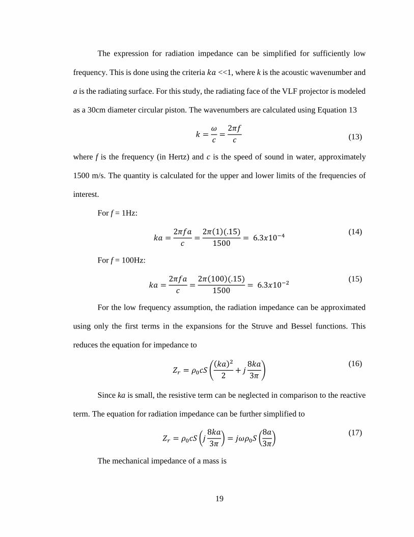
The expression for radiation impedance can be simplified for sufficiently low

frequency. This is done using the criteria 𝑘𝑎 <<1, where k is the acoustic wavenumber and

a is the radiating surface. For this study, the radiating face of the VLF projector is modeled

as a 30cm diameter circular piston. The wavenumbers are calculated using Equation 13

𝑘 =

𝜔

𝑐=

2𝜋𝑓

𝑐 (13)

where f is the frequency (in Hertz) and c is the speed of sound in water, approximately

1500 m/s. The quantity is calculated for the upper and lower limits of the frequencies of

interest.

For f = 1Hz:

𝑘𝑎 =

2𝜋𝑓𝑎

𝑐=

2𝜋(1)(.15)

1500= 6.3𝑥10−4

(14)

For f = 100Hz:

𝑘𝑎 =

2𝜋𝑓𝑎

𝑐=

2𝜋(100)(.15)

1500= 6.3𝑥10−2

(15)

For the low frequency assumption, the radiation impedance can be approximated

using only the first terms in the expansions for the Struve and Bessel functions. This

reduces the equation for impedance to

𝑍𝑟 = 𝜌0𝑐𝑆 (

(𝑘𝑎)2

2+ 𝑗

8𝑘𝑎

3𝜋)

(16)

Since ka is small, the resistive term can be neglected in comparison to the reactive

term. The equation for radiation impedance can be further simplified to

𝑍𝑟 = 𝜌0𝑐𝑆 (𝑗

8𝑘𝑎

3𝜋) = 𝑗𝜔𝜌0𝑆 (

8𝑎

3𝜋)

(17)

The mechanical impedance of a mass is

20

Therefore, the radiation impedance of a low frequency can be simplified to an added mass.

𝑀𝑟 = 𝜌0𝑆 (

8𝑎

3𝜋)

(19)

This radiation mass is added to the mass of the piston radiating face to calculate the total

added mass being pushed by the LM2:

𝑀𝑡𝑜𝑡𝑎𝑙 = 𝑀𝑝𝑖𝑠𝑡𝑜𝑛 + 𝑀𝑟 (20)

Using the total mass and the LM2’s performance curves, a displacement curve for the VLF

projector is generated, as shown in Figure 16.

Figure 16: A plot of displacement amplitude for an added mass of 14.1 kg. This curve was

generated using the total mass (piston and radiation mass) and the Bose performance curves

of the LM2 MMA.

The peak displacement amplitude, 𝑋0, is integrated to calculate peak velocity 𝑈0.

𝑈0 = 2𝜋𝑓𝑋0 (21)

𝑍 = 𝑗𝜔𝑀 (18)

21

Peak velocity is multiplied by the area of the radiating surface to calculate volume

velocity, 𝑄0.

𝑄0 = 𝑈0𝜋𝑎2 (22)

From volume velocity, radiated power, Π, is calculated using equations

𝛱 =

1

2𝑈0

2𝑅𝑟 (23)

𝑅𝑟 = 𝜌0𝑐(𝑘𝑆)2/4𝜋 (24)

which can be simplified to

𝛱 =

1

8𝜌0𝑐(𝑘𝑄0)2

(25)

Finally, acoustic source level, SL, can be calculated using the equation

𝑆𝐿 = 10 𝑙𝑜𝑔10 (𝜌0𝑐𝛱

4𝜋∗10−12) (26)

A plot of the modeled source level can be seen in Figure 17.

Figure 17: A plot of expected source level for the VLF projector using equations for a

simple point source. The shape is defined by a displacement limited region where the

acoustic performance is limited by the peak displacement of the MMA and the force limited

region where the acoustic performance is limited by the peak force of the MMA.

Displacement

Limited Region Force Limited

Region

22

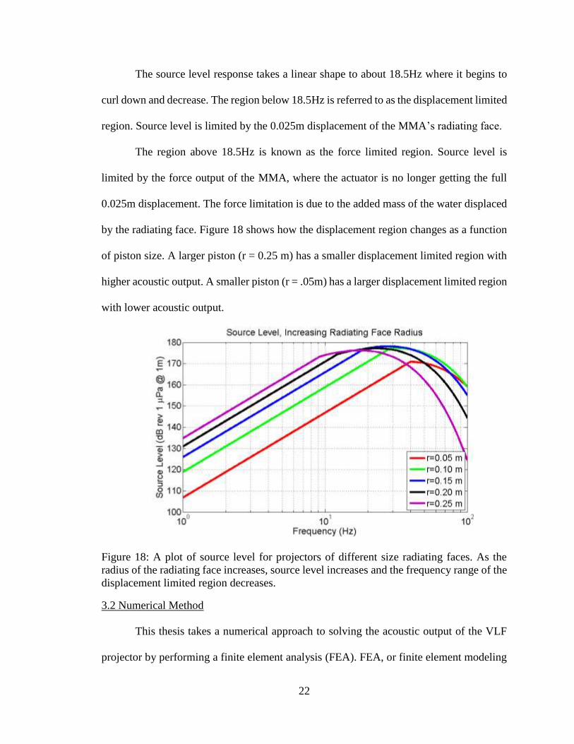
The source level response takes a linear shape to about 18.5Hz where it begins to

curl down and decrease. The region below 18.5Hz is referred to as the displacement limited

region. Source level is limited by the 0.025m displacement of the MMA’s radiating face.

The region above 18.5Hz is known as the force limited region. Source level is

limited by the force output of the MMA, where the actuator is no longer getting the full

0.025m displacement. The force limitation is due to the added mass of the water displaced

by the radiating face. Figure 18 shows how the displacement region changes as a function

of piston size. A larger piston (r = 0.25 m) has a smaller displacement limited region with

higher acoustic output. A smaller piston (r = .05m) has a larger displacement limited region

with lower acoustic output.

Figure 18: A plot of source level for projectors of different size radiating faces. As the

radius of the radiating face increases, source level increases and the frequency range of the

displacement limited region decreases.

3.2 Numerical Method

This thesis takes a numerical approach to solving the acoustic output of the VLF

projector by performing a finite element analysis (FEA). FEA, or finite element modeling

23

(FEM), is utilized in engineering when mathematic expressions for geometries, loading, or

material properties are complicated such that the closed form analytical solution does not

exist. FEA was developed as an approximation technique exploiting Hooke’s law which

states “For small deformations of the object, the amount of deformation/ displacement is

directly proportional to the deforming force or load” [13]. Hooke’s law is defined in matrix

form as

{𝐹} = [𝑘]{𝑥} (27)

where {𝐹} is a force vector, {𝑥} is a displacement vector, and [𝑘] is the constant of

proportionality i.e. stiffness matrix. In a finite element model, large complex geometries

are divided into a finite number of small simple geometric sub regions called elements.

FEA solvers sum up the individual behaviors of each element to predict the behavior of the

entire physical system.

Elements are connected to each other at nodes. A set of connected elements is called

a mesh. Figure 19 shows examples of meshes containing 2D elements with three nodes

(triangular mesh) and four nodes (quadrilateral mesh).

Figure 19: Mesh containing elements with 3 nodes (left) and 4 nodes (right).

Hooke’s law is analyzed at the nodal level. Each node is a coordinate point where

degrees of freedom are defined. Each element is the mathematical relation that defines how

the motion of one node relates to the rest of the nodes on the element through its material

24

properties. When performing an analysis, select nodes are prescribed force and

displacements known as defined loads and boundary conditions. When an FEA simulation

is performed, the effect of the defined loads is calculated for all nodes in the model.

The method of FEA has evolved to solve acoustic problems the same way it is used

to solve Hooke’s equation. The equation of motion for a damped system excited by a force

is [14]

𝐹 = 𝑚�̈� + 𝑐�̇� + 𝑘𝑥 (28)

where 𝐹 is force, 𝑚 is mass, 𝑐 is the damping parameter, 𝑘 is the stiffness parameter, and

𝑥 is displacement. For studies of pure harmonics, force and displacement can be written as

𝐹 = 𝐹𝑒𝑗𝜔𝑡, 𝑥 = 𝑥𝑒𝑗𝜔𝑡 (29)

where j is the imaginary number ( √−1 ) and 𝜔 is angular frequency. Equation 28 can be

rewritten as

𝐹𝑒𝑗𝜔𝑡 = [−𝜔2𝑚 + 𝑗𝜔𝑐 + 𝑘]𝑥𝑒𝑗𝜔𝑡 (30)

{𝐹} = [−𝜔2𝑚 + 𝑗𝜔𝑐 + 𝑘]{𝑥} (31)

Equation 31 is the equation of motion for a harmonic system written in a form

similar to Hooke’s law solved by FEA, Equation 27. Values for stiffness, mass, and

damping are all included in the constant of proportionality matrix.

In the problem of calculating the acoustic output of a projector, the response of the

fluid (the acoustic domain) to the oscillatory motion of the VLF projector’s radiating face

and housing is examined. This kind of FEA is known as a fluid-structure interaction (FSI).

In an FSI problem, motion of a structure and fluid are coupled by tying nodes on the

boundary together. The matrix equations that couple a fluid structure interaction are written

as [15]

25

[𝑀𝑠]{�̈�} + [𝐾𝑠]{𝑥} = {𝐹𝑠} + [𝑅]{𝑃} (32)

[𝑀𝑓]{�̈�} + [𝐾𝑓]{𝑃} = {𝐹𝑓} + 𝜌[𝑅]𝑇{�̈�} (33)

where [𝑀] is the mass matrix, [𝐾] is the stiffness matrix, [𝑅] is the coupling matrix, 𝜌 is

density of the medium, and {𝑃} is the pressure vector.

The first step to perform an FEA is to set up the geometry. A solid model of the

VLF projector housing and radiating face is created in SolidWorks, Figure 20.

26

Figure 20: SolidWorks model of VLF projector housing and radiating face

The SolidWorks model is imported into HyperMesh, an FEA preprocessing

software that defines the problem for the FEA solver (Abaqus) by assigning the material

properties, boundary conditions, and desired solver outputs. Once imported, an

axisymmetric model is created from the SolidWorks model of the projector, shown in

Neoprene suspension

Radiating face

Direction of actuation

27

Figure 21. The VLF projector is the “structure” in the FSI model. An additional geometry

is created for the acoustic domain where Abaqus will solve for acoustic pressure. The

acoustic domain is the blue semicircle surrounding the projector in Figure 21. The radius

of the acoustic domain is 2 meters. The acoustic domain is the “fluid” in the FSI model.

Figure 21: Axisymmetric model of VLF projector (left) and acoustic domain (right)

Once all the geometries for the model are defined, the next step is to mesh the

model. The structure is defined using CAX4R elements. These are continuum (C), or solid,

axisymmetric (AX) quadrilateral (4 node) elements that use a reduced (R) integration

method for calculating the stiffness matrix. There are two active degrees of freedom for the

nodes of these elements: displacement in the x and displacement in the y in meters (m).

Radiating face Neoprene suspension

Direction of actuation

28

Designing a mesh requires a compromise between accuracy of the results and

computational time to run the analysis. In FEA, the DOF is calculated for each node. A

course mesh with large elements will contain a small number of nodes resulting in a small

number of equations to solve. An analysis with a course mesh will have a short computation

time but numerical approximations may not be accurate. A fine mesh with small elements

will contain a large number of nodes resulting in a large number of equations to solve. An

analysis with a fine mesh should yield high resolution results, but may take more time to

compute.

In order to create a mesh that is both accurate and computationally efficient, a

method of mesh refinement is used once the model is constructed. In this method, the model

is first made with a course mesh, then reran with finer and finer meshes, comparing the

results between models of different meshes until there is a point of diminishing returns on

the accuracy. To begin, the mesh is designed using three elements through the thickness of

the thinnest wall of the structure. The structure meshed can be seen in Figure 22.

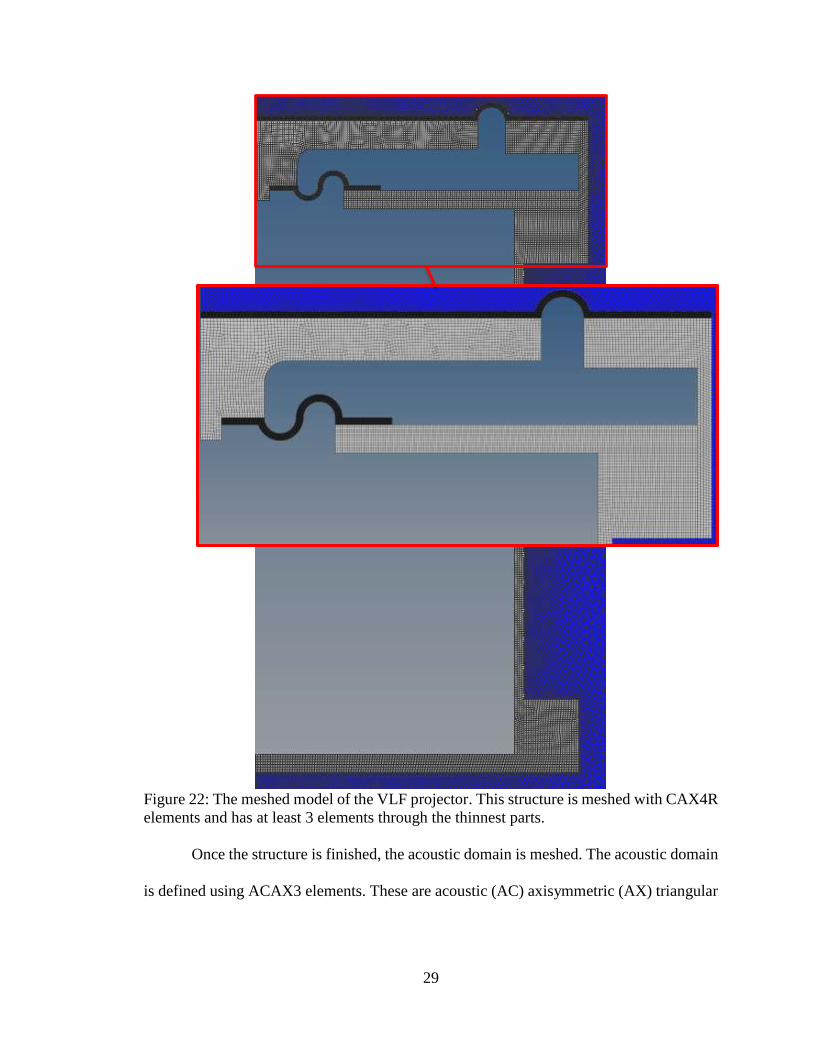
29

Figure 22: The meshed model of the VLF projector. This structure is meshed with CAX4R

elements and has at least 3 elements through the thinnest parts.

Once the structure is finished, the acoustic domain is meshed. The acoustic domain

is defined using ACAX3 elements. These are acoustic (AC) axisymmetric (AX) triangular

30

(3 node) elements. The nodes of these elements only record one active degree of freedom:

acoustic pressure (POR) in Pascals.

It is difficult to perform a finite element modeling on acoustics of SONAR

transducers for two reasons. One reason is that mesh must be small such that there are

multiple nodes per wavelength. Equation 5 shows for a constant speed of sound, frequency

is inversely proportional to wavelength. Higher frequency SONAR means shorter

wavelength and a finer mesh.

The second reason is acoustic measurements must be taken in the far field, defined

as [16]

𝑟 =

𝐴

𝜆

(34)

where 𝑟 is the transition region between the near field and the far field, 𝜆 is wavelength,

and 𝐴 is the area of the circular piston. For a transducer of constant size, as wavelength is

decreased (frequency increased), the distance to the far field increases, demanding a larger

acoustic domain for the model.

An FEA analysis that requires both a large acoustic domain and a fine mesh can

become very computationally demanding due to the number of equations that must be

solved. This is not an issue as this application is low frequency (long wavelength).

Source level is recorded one meter from the radiating face. A node is created one

meter from the projector’s radiating face in the fluid domain. For the shortest wavelength,

𝜆 = 15𝑚, the transition region is calculated

𝑟 =

𝜋(. 15)2

15= 4.71𝑥10−3

(35)

Since 1 meter is greater than r, pressure recorded is in the far field.

31

Mesh must be small such that there are multiple elements per wavelength. The

minimum number is two elements per wavelength, but the recommended is three to five

[17]. This results in about six to ten nodes per wavelength. While the criteria would be

difficult to meet for a high frequency applications, the shortest wavelength in this study is

15 meters long. The meshed acoustic domain is shown in Figure 23. The elements grow

from the center of the domain with the largest elements at the outer edge of the acoustic

domain. These large elements are 1/25th the size of the smallest wavelength, making the

domain more than suitable for this application.

.

Figure 23: The meshed acoustic domain. This fluid is meshed with ACAX3 elements and

element size grows as it approaches the outer boundary of the domain.

Material properties are defined for all parts of the structure and the fluid. Table 2

shows properties for the butyl rubber suspension pieces and the stainless steel housing.

Table 3 shows the material properties for the acoustic domain water [18].

32

Density (kg/𝑚3) Young's Modulus (GPa) Poisson's ratio

Stainless Steel 7800 0.198 0.289

Butyl Rubber 910 0.002 0.3

Table 2: Material properties for the structure in the numerical model. The structure refers

to the VLF projector.

Density (kg/𝑚3) Bulk Modulus Speed of Sound (m/s)

Water 1000 2.15 1500

Table 3: Material properties of the fluid in the numerical model. The fluid refers to the

acoustic domain.

Loads and boundary conditions are then defined in HyperMesh. The model is

designed to solve for acoustic pressure in the fluid domain due to actuation of the

projector’s radiating face. In order to study the interactions between the fluid and structure,

a tie constraint (Abaqus keyword TIE) [19] is applied at the surface. This is the continuity

constraint that ties all nodes on the interface between the fluid and structure together.

Abaqus computes the coupling matrices from Equations 32 and 33 for these nodes. The

structure is set as the “master” and the fluid is set at the “slave.” Therefore, the motion of

all nodal values on the fluid-structure interface is due to the motion of the structure. A

nonreflecting surface impedance boundary condition (Abaqus keyword SIMPEDANCE)

is applied to the exterior boundary of the acoustic to simulate an infinitely large acoustic

domain. A point mass node (Abaqus keyword MASS) is placed at the center of the

projector to simulate the mass of the MMA. To simulate actuator motion, a motor shaft is

created as a connector element between two nodes on the axis of symmetry (Abaqus

Keyword CONN2D2) and displacement motion (Abaqus keywords CONNECTOR

33

MOTION) is prescribed to simulate a displacement of the shaft. The boundary conditions

are described visually in Figure 24.

Figure 24: HyperMesh model with callouts describing boundary conditions. Nodes on the

fluid structure interface are tied together using a tie constraint (Abaqus keyword TIE). To

simulate an infinite acoustic domain, a nonreflective boundary is applied to the edge of the

acoustic domain (Abaqus keyword SIMPEDANCE). A point mass node (Abaqus keyword

MASS) is placed at the center of the projector to simulate the mass of the MMA. To

simulate actuator motion, a motor shaft is created as a connector element between two

nodes on the axis of symmetry (Abaqus Keyword CONN2D2) and a displacement motion

KINNCOUP

CONN2D2 & CONNECTOR MOTION

MASS

TIE

SIMPEDANCE

KINNCOUP

34

(Abaqus keywords CONNECTOR MOTION) is prescribed to apply a displacement to the

shaft.

The radiating face is driven with the same displacement amplitudes from the

analytical model. A tabular version of amplitude data, Figure 16, is loaded into HyperMesh

as the prescribed motion for the connector shaft. The model from HyperMesh is loaded

into Abaqus to run the analysis. The model outputs a peak pressure value for the acoustic

element located 1 meter from the radiating face for each input frequency. The peak value

for pressure (Abaqus history output POR) is used to calculate acoustic source level (SL)

using the equation

𝑆𝐿 = 20𝑙𝑜𝑔10 (

𝑃𝑂𝑅/√2

1 𝜇𝑃𝑎)

(36)

The numerical calculation for source level is plotted with the analytical result in Figure 25.

Figure 25: The plot of the analytical and Abaqus results.

35

The calculated SL shows the Abaqus output of the model having a greater value for

acoustic pressure than the analytical model. One hypothesis for the discrepancy is

“effective radius.” The radius of the piston is 0.15 m, but the radius of the piston plus the

suspension is 0.175 m. The suspension contributing to a larger surface area than just the

piston itself could account for the higher SL. In Figure 26, the analytical model is rerun

for the effective radius of 0.175m.

Figure 26: Source level plotted for an analytical analysis performed with a radiating face

of radius 0.15m (blue) and 0.175m (black) against the numerical results. This plot supports

the hypothesis that the suspension geometry could contribute to a higher SL output.

For acoustic outputs in the displacement limited region, the numerical results are

somewhere between the analytical results for a piston of a radius r=0.15m and r=0.175m.

This supports the hypothesis that the suspension plays a role in increasing the acoustic

pressure output, but not to the point where it is the same as having a piston of radius of

36

0.175m. Because the FEA model is displacement driven with the displacement parameters

from the analytical model for 0.15m, the transition to the force limited region occurs at the

same frequency in the numerical model and the analytical model for 0.15m –not the 0.175m

model.

37

CHAPTER 4

Experimental Testing

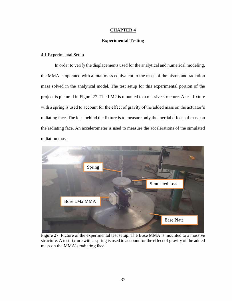
4.1 Experimental Setup

In order to verify the displacements used for the analytical and numerical modeling,

the MMA is operated with a total mass equivalent to the mass of the piston and radiation

mass solved in the analytical model. The test setup for this experimental portion of the

project is pictured in Figure 27. The LM2 is mounted to a massive structure. A test fixture

with a spring is used to account for the effect of gravity of the added mass on the actuator’s

radiating face. The idea behind the fixture is to measure only the inertial effects of mass on

the radiating face. An accelerometer is used to measure the accelerations of the simulated

radiation mass.

Figure 27: Picture of the experimental test setup. The Bose MMA is mounted to a massive

structure. A test fixture with a spring is used to account for the effect of gravity of the added

mass on the MMA’s radiating face.

Spring

Simulated Load

Bose LM2 MMA

Base Plate

38

The equipment used to drive the actuator is pictured in Figure 28. A signal generator

is used to apply a +/- 10 V command signal to the Bose amplifier. The Bose amplifier

drives the MMA with a current proportional to the command voltage (4.7A/V).

Figure 28: A picture of the equipment to drive the MMA. A signal generator is used to

apply a +/- 10 V command signal to the Bose amplifier that drives the MMA with a high

voltage signal. An oscilloscope is used to verify the signals being sent to the MMA.

Figure 29 shows the PXI chassis that is used to record the experimental data. Four

channels are recorded on the PI-4462 card: acceleration, command voltage, voltage across

the actuator’s coils, and current applied to the actuator. Acceleration is measured with a

Kistler Model 8604B500 accelerometer with a sensitivity of 10mV/g. Command voltage

is recorded directly from the Wavetek function generator. Current is monitored using a

Pearson Electronic Inc. wideband current transformer with a transfer function of 0.1Volts/

Amp. The MMA’s drive voltage is recorded by probing the voltage across the coils and

attenuating the voltage by 200x using a Fluke DP120 voltage probe.

Bose Amplifier

Oscilloscope

Signal Generator

39

Figure 29: A picture of the PXI chassis that records the experimental data. Four channels

with recorded on the PI-4462 card: acceleration, command voltage, voltage across the

MMA’s coils, and current applied to the actuator.

4.2 Experimental Analysis

From acceleration data and frequency information, the displacement 𝑋0 of the

MMA is calculated using the equation

𝑋0 = −𝑎

𝜔2 (37)

where ω is the angular frequency and 𝑎 is acceleration. For this experiment, five trials were

taken at 13 frequencies: 5, 7, 10, 15, 18, 20, 30, 45, 50, 60, 70, 80, 90, Hz. The mean value

for displacement amplitude was calculated using the 1- α confidence interval [20]

[(�̅� −

𝑠𝑡𝑛;

𝛼2

√𝑁) ≤ 𝜇𝑥 < (�̅� +

𝑠𝑡𝑛;

𝛼2

√𝑁)] ; 𝑛 = 𝑁 − 1

(38)

40

where 𝜇𝑥 is the mean value based on sample mean �̅� and standard deviation s from sample

size N. The critical value 𝑡 depends on the degrees of freedom in the study (𝑛) and an alpha

value (𝛼). The degree of freedom is the number of independent pieces of information within

the statistical analysis. For confidence interval, the degree of freedom is one less than the

sample size. Alpha is the percentage of confidence subtracted from one.

The purpose of the confidence interval is to estimate a repeatable maximum

displacement for the actuator from a sample number of tests for maximum displacement.

For a sample size of N = 5 and a 95% confidence interval (α = .05),

[(�̅� −

𝑠𝑡4;.025

√5) ≤ 𝜇𝑥 < (�̅� +

𝑠𝑡4;.025

√5)]

(39)

Using Student’s t-table, 𝑡4;.025 = 2.776

[(�̅� − 1.2415𝑠) ≤ 𝜇𝑥 < (�̅� + 1.2415𝑠)] (40)

Mean values and confidence intervals are plotted in Figure 30 and can be seen in

tabular form in Table 4. Figure 31 plots the experimental data against the theoretical

displacements from Figure 16.

41

Figure 30: Plot of the mean values and confidence intervals for experimental displacement

of the MMA. The values are plotted against theoretical displacement values.

Frequency (Hz) Mean displacement, �̅� (m) 𝑠𝑡4;.025

√5 (m)

5 1.24E-02 7.24E-05

7 1.20E-02 2.11E-04

10 1.20E-02 1.04E-04

15 1.22E-02 9.24E-05

18 1.18E-02 2.88E-04

20 1.07E-02 3.20E-04

30 4.55E-03 3.25E-04

45 1.74E-03 1.28E-04

50 1.31E-03 5.61E-05

60 6.96E-04 1.75E-04

70 3.65E-04 8.52E-05

80 2.00E-04 1.89E-05

42

90 8.65E-05 1.62E-05

Table 4: Tabular data for experimental displacement of MMA radiating face

A regression curve is constructed from the experimental data (as illustrated in

Figure 31). The regression is a piecewise function with a constant displacement from 1Hz

to 18.5Hz and a decreasing exponential from 18.5Hz to 100Hz.

Figure 31: Plot of a regression fit to the experimental data (green). The regression is a

piecewise function that is constant below 18.5 kHz and a decreasing exponential above

18.5 kHz. The regression fit is plotted against the theatrical displacements for a 14.1kg

added mass based on the Bose performance curves.

The analytical acoustic analysis was rerun using the experimental data regression

curve from Figure 31. Figure 32 shows that source levels calculated using the experimental

data and source levels calculated using the Bose performance curves are within half a

decibel in the displacement limited region (below 18.5Hz) and within one decibel in the

force limited region (above 18.5Hz). Comparing source level based on the Bose

specification curves for displacement with source level based on the displacement curve

43

constructed from the experimental data validates the results of the two models that are

based on the Bose performance curves.

Figure 32: Plot of acoustic source level using the experimental fit of displacement (green)

against the source level estimated in the analytical analysis using the Bose specifications

for displacement.

44

CHAPTER 5

Future work

This thesis investigates the feasibility of implementing a moving magnet actuator

(MMA) as the motor driver for a low frequency underwater acoustic projector. The analysis

was based on displacement and force outputs provided in the product technical

specifications and was verified experimentally. This analysis is only the first step in the

design, fabrication, and calibration of an underwater transducer.

The next step for building the projector would be a detailed design for a housing.

The SolidWorks designs delivered in this report were simplified solid models intended only

to be used for the FEA modeling. When the housing is designed for manufacturing of parts,

the designer will have to focus on designing a watertight housing. The Bose MMA is an

expensive piece of equipment; precautions must be taken to ensure the housing will not

flood when placed in the water.

Another design parameter to investigate is how the projector will compensate for

hydrostatic pressure. Since the primary intention of this projector is to use it as a sound

source for calibrating a towed array, the projector only needs to be pressure compensated

to a specific test depth of about 15 meters.

The design of the operational projector will also have to factor in designing cabling.

The current model of the MMA came with a 5 foot cable from the Bose amplifier to the

actuator. If the MMA is to be used as a projector at a test depth, a new set of cabling must

be designed.

Another design factor for the mechanical design of the projector is how the heat

generated from the MMA is dissipated. Currently, fans cool heat sinks attached to the coils

45

of the actuator. When the MMA is placed inside a housing, a new heat dissipation system

must be designed. This could be as simple as designing heat sinks that span to the wall of

the housing.

Once the projector is built, it must then be calibrated. Since the frequency range is

1-100Hz, long wavelengths will make it difficult to get an accurate transmitting voltage

response (TVR) of the projector due to any reflections of sound in the Leesburg test facility.

It may be necessary to imbed an accelerometer in the radiating face of the projector as a

feedback for how the projector is operating at depth.

46

CHAPTER 6

Conclusion

The U.S. Navy has developed a passive calibration method at the Leesburg test

facility for frequencies below 60Hz. In the passive method, ambient noise in the facility is

used as the calibration sound source. The Navy is looking to replace this method with a

reference projector calibration method. Unfortunately, the Navy does not currently have a

reliable sound source at this frequency.

The data presented in this work shows the feasibility of implementing a moving

magnet actuator (MMA) as the motor force in an underwater acoustic transducer. Based on

the MMA’s force and displacement specifications, a sound pressure level was calculated

using two methods. The first method was an analytical method using equations for a simple

sound source. This analysis was done using the software program Matlab. The second

analysis was a numerical analysis: a fluid-structure interaction model where the acoustic

medium was the fluid and the projector was the structure. Modeling efforts estimate a

source level of over 125dB re 1 𝜇𝑃𝑎 @1m at 1Hz and over 180 dB re 1 𝜇𝑃𝑎 @1m at 30Hz.

These numbers can be compared to spectrum levels of the spring at thesis frequencies

which are 91 dB re 1 𝜇𝑃𝑎/ √𝐻𝑧 at 1 Hz and 87 dB re 𝜇𝑃𝑎/ √𝐻𝑧 at 30 Hz.

This thesis also covered experimentally testing the Bose moving magnet actuator.

The experimental efforts found the MMA operates at displacements necessary to achieve

sound pressure levels calculated from the analytical and numerical models.

Lastly, future work was discussed. This thesis is just the preliminary study on what

kind of acoustic output can be achieved using a moving magnet actuator. There are still

many factors that will play a role in building a transducer. These factors include building

47

a housing that can be lowered to the necessary test depth without flooding and

compensating the projector for hydrostatic pressure.

48

LIST OF REFERENCES

[1] Underwater Sound Reference Division, “Leesburg Facility” [online] Available:

http://www.navsea.navy.mil/Home/Warfare-Centers/NUWC-Newport/What-We-

Do/Detachments/Underwater-Sound-Reference-Division/Leesburg-Facility/

[Accessed: Mar.2017].

[2] S. E. Crocker, R.R. Smalley, "Calibration of a Digital Hydrophone Line Array at Low

Frequency," in IEEE Journal of Oceanic Engineering , vol.41, no.4, pp.1020-1027

[3] R. P. Hodges, Underwater acoustics: analysis, design, and performance of sonar.

Chichester, West Sussex England: J. Wiley, 2010, p.p. 3-4.

[4] J. Bourne, J. Sacks, and C. Bradley, E.encyclopedia: Energy Waves. New York:

Dorling Kindersley, 2003

[5] R. Feynman, Lectures in Physics, Volume 1, Chapter 47: Sound. The wave equation,

Caltech 1963

[6] W.C. Lane “The Wave Equation and Its Solutions”. Michigan State University, 2002

[7] B. Lunardini “A Study of Speakers and their Harmonics” M.S. Thesis, University of

Illinois, 2004

[8] R.W., Timme, A.M., Young, & Blue J.E. “Transducer needs for low-frequency sonar”

presented at the Second international workshop on power transducers for sonics and

ultrasonics, France, 1990.

[9] D. B. Hiemstra, G. Parmar and S. Awtar, "Performance Tradeoffs Posed by Moving

Magnet Actuators in Flexure-Based Nanopositioning," in IEEE/ASME Transactions on

Mechatronics, vol. 19, no. 1, pp. 201-212, Feb. 2014.

[10] Bose Corporation, “ElectroForce Linear Motion Systems” datasheet, 2014.

[11] Bose Corporation, “Performance Curves, LM3000-25” datasheet, 2014.

[12] L. E. Kinsler, A.R. Frey, Fundamentals of acoustics. New York: John Wiley & Sons,

2000, pp. 185-189.

[13] D. Thakore, Finite Element Analysis with Open Source Software, 2th ed. Brisbane,

Australia: Moonish Enterprises Pty Ltd, 2014, pp. xiii-xv.

[14] H. Gavin. CEE 541. Lecture, Topic: “Vibrations of Single Degree of Freedom

Systems.” Structural Dynamics Department of Civil and Environmental Engineering

Duke University, Fall 2016

[15] C. H. Sherman and J. L. Butler, Transducers and Arrays for Underwater Sound, New

York: Springer, 2007

[16] R. J. Urick, Principles of underwater sound. Los Altos, CA: Peninsula, 1988

[17] P. Schmiechen. “Travelling wave speed coincidence,” PhD Dissertation, Imperial

College of Science, Technology and Medicine, University of London, 1997.

[18] Dassault Systèmes, 2013. Abaqus 6.13 Online Documentation.

49

[19] Automation Creations, Inc.. (2009). MatWeb, Your Source for Materials Information.

[online] Available: http://www.matweb.com/ [Accessed: Mar.2017]

[20] J. S. Bendat, Random Data Analysis and Measurement Procedures. New Jersey:

Wiley, 2010, pp.97

50

APPENDIX

This Appendix contains a list of the MATLAB scripts and the HyperMesh input deck

used in the thesis, along with a brief description of what each one does.

AnalyticalandNumericalCode.m

This script is used to calculate the analytical solution from fundamental equations for an

acoustic point source. The script also loads numerical outputs from Abaqus to compare

to the numerical results.

DataCollection.m

This script is used to record the experimental data on the PXI chassis.

MMA_processing.m

This script is used to process the experimental data and compare it to the analytical

results.

VLF_FEAInputFile.inp

Input file exported from HyperMesh and input into Abaqus to solve the FEA problem.

51

BIBLIOGRAPHY

Automation Creations, Inc.. (2009). MatWeb, Your Source for Materials Information.

[online] Available: http://www.matweb.com/ [Accessed: Mar.2017]

Bose Corporation, “ElectroForce Linear Motion Systems” datasheet, 2014.

Bose Corporation, “Performance Curves, LM3000-25” datasheet, 2014.

C. H. Sherman and J. L. Butler, Transducers and Arrays for Underwater Sound, New York:

Springer, 2007

D. B. Hiemstra, G. Parmar and S. Awtar, "Performance Tradeoffs Posed by Moving

Magnet Actuators in Flexure-Based Nanopositioning," in IEEE/ASME Transactions on

Mechatronics, vol. 19, no. 1, pp. 201-212, Feb. 2014.

D. Thakore, Finite Element Analysis with Open Source Software, 2th ed. Brisbane,

Australia: Moonish Enterprises Pty Ltd, 2014, pp. xiii-xv.

Dassault Systèmes, 2013. Abaqus 6.13 Online Documentation.

H. Gavin. CEE 541. Lecture, Topic: “Vibrations of Single Degree of Freedom Systems.”

Structural Dynamics Department of Civil and Environmental Engineering Duke

University, Fall 2016

J. Bourne, J. Sacks, and C. Bradley, E.encyclopedia: Energy Waves. New York: Dorling

Kindersley, 2003

J. S. Bendat, Random Data Analysis and Measurement Procedures. New Jersey: Wiley,

2010, pp.97

L. E. Kinsler, A.R. Frey, Fundamentals of acoustics. New York: John Wiley & Sons,

2000, pp. 185-189.

P. Schmiechen. “Travelling wave speed coincidence,” PhD Dissertation, Imperial College

of Science, Technology and Medicine, University of London, 1997.

R. Feynman, Lectures in Physics, Volume 1, Chapter 47: Sound. The wave equation,

Caltech 1963

R. J. Urick, Principles of underwater sound. Los Altos, CA: Peninsula, 1988

R. P. Hodges, Underwater acoustics: analysis, design, and performance of sonar.

Chichester, West Sussex England: J. Wiley, 2010, p.p. 3-4.

R.W., Timme, A.M., Young, & Blue J.E. “Transducer needs for low-frequency sonar”

presented at the Second international workshop on power transducers for sonics and

ultrasonics, France, 1990.

S. E. Crocker, R.R. Smalley, "Calibration of a Digital Hydrophone Line Array at Low

Frequency," in IEEE Journal of Oceanic Engineering , vol.41, no.4, pp.1020-1027

Underwater Sound Reference Division, “Leesburg Facility” [online] Available:

http://www.navsea.navy.mil/Home/Warfare-Centers/NUWC-Newport/What-We-

Do/Detachments/Underwater-Sound-Reference-Division/Leesburg-Facility/

[Accessed: Mar.2017].

52

W.C. Lane “The Wave Equation and Its Solutions”. Michigan State University, 2002