implementation of massive artificial neural networks with cuda

13

Implementation of Massive Artificial Neural Networks with CUDA

Domen Verber University of Maribor

Slovenia

1. Introduction

People have always been amazed with the inner-workings of the human brain. The brain is

capable of solving variety of problems that are unsolvable by any computers. Is capable of

detecting minute changes of light, sound or smell. It is capable of instantly recognizing a

face, to accurately read the handwritten text, etc. The brain is the centre of what we call

human intelligence and self-awareness. This is not limited only to the human brain. A bee,

for example, has a brain that is only a fraction the size compared to the human brain.

Nevertheless, the bee able of detecting nectar over long distances; it is capable to orient itself

in space and find its way back to the beehive, and it is capable of transferring the

information about nectar locations to other bees though a well-choreographed dance.

The basic unit of the nervous system is the neuron. A group of neurons build a neuronal

network. In general, a neural network is a parallel system, capable of resolving problems

that linear-computing cannot. Neural nets are used for signal processing, pattern

recognition, visual and speech processing, in medicine, in business, etc.

The techniques of the neural networks are a part of a machine-learning paradigm. Using

this, a system should find solutions for certain problems based only on empirical data, using

unknown underlying probability distribution. In addition to this, a vast number of research

has been done in the field of artificial neural networks, in order to better understand the

human brain, itself. For example, in the Blue Brain Project, the goal is to reconstruct the

brain piece by piece and build a virtual brain within supercomputer (BBP, 2011). This

approach tries to emulate the human brain very accurately, and requires considerable

computing power. Each simulated neuron requires the equivalent of a laptop computer.

Several programming libraries and tools exists, which allow for building artificial neural

networks of moderate sizes. In addition, several experiments have been where the neurons

are emulated within hardware.

This exposure presents a study how to use massive parallel programming on general PCs for artificial neural networks (ANN), which utilizes the processing power and highly parallel computer architectures of graphic processor units (GPU). GPUs on mass-market graphical cards may greatly outperform general processors for some type of applications, both in computation power and in memory bandwidth. The graphic processor consists of a large number of processing cores that may perform a large number of tasks, in parallel. The execution of artificial neural networks is an intrinsically parallel problem. Therefore, parallel

www.intechopen.com

Cutting Edge Research in New Technologies

278

computational architectures, such as GPUs, lead to a great improvement in speed. Until recently, the programmers of ANN could only harness this processing power with especially prepared graphical applications. What is new is that the newest GPU architectures allow for a more general approach to ANN programming, without taking into consideration the graphical aspects of GPUs. One general-purpose parallel computing architecture is CUDA (Compute Unified Device Architecture), as developed by the Nvidia GPU manufacturer. Different aspects of ANN implementation using CUDA are discussed later. A much greater performance of ANN can be achieved by better understanding the particularities and limitations of CUDA. The next section presents some biological background of neurons and neural network. Later, different implementation techniques are identified for artificial neural networks. The main section explains section, the implementation of ANN with the CUDA development toll. In conclusion, several experiments are demonstrated and several implementation techniques for large ANN are compared.

2. Biological background of neurons and neural networks

The biological aspects of the nervous system are studied since ancient times. Modern understanding of the neurons started toward the end of the 19th century. Advances in technology, especially regarding brain scanning techniques, the in-vivo observation of mammalian and human brains, etc., allows scientists to determine a detailed understanding of neurons and biological neural networks. In this section, only the brief introduction is given, as relevant to the rest of the matter, is given. For a detailed description regarding biological features of neurons and the nervous system, see (Nicholls et al., 2001). For a detailed survey of the theoretical neuroscience, see (Dayan & Abbot, 2001).

2.1 Neurons

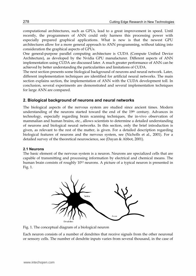
The basic element of the nervous system is a neuron. Neurons are specialized cells that are capable of transmitting and processing information by electrical and chemical means. The human brain consists of roughly 1012 neurons. A picture of a typical neuron is presented in Fig. 1.

Fig. 1. The conceptual diagram of a biological neuron

Each neuron consists of a number of dendrites that receive signals from the other neuronal or sensory cells. The number of dendrite inputs varies from several thousand, in the case of

www.intechopen.com


279

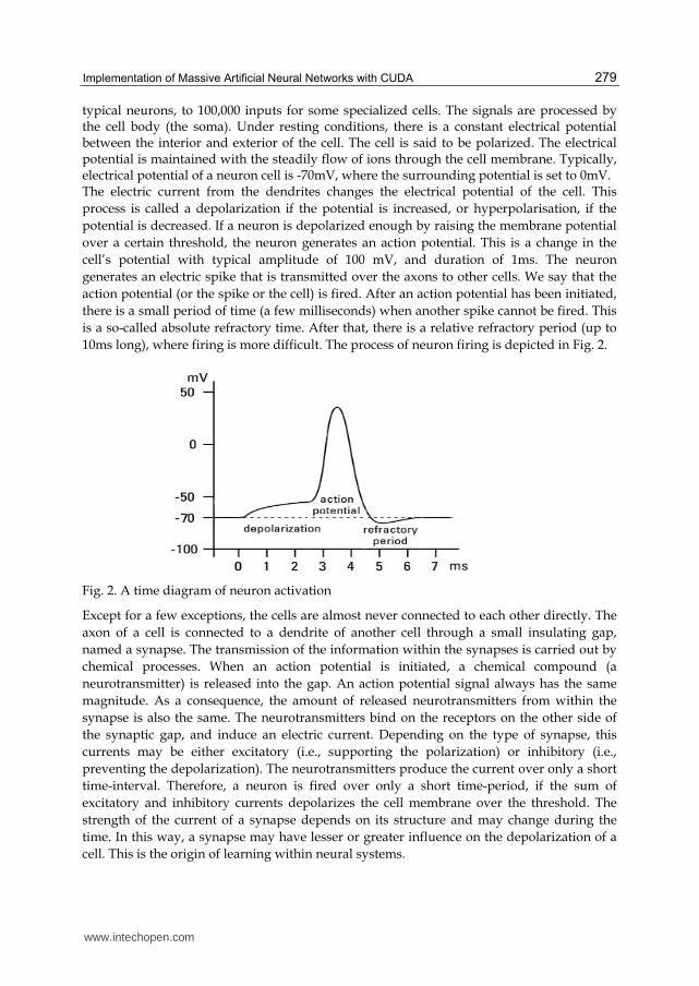
typical neurons, to 100,000 inputs for some specialized cells. The signals are processed by the cell body (the soma). Under resting conditions, there is a constant electrical potential between the interior and exterior of the cell. The cell is said to be polarized. The electrical potential is maintained with the steadily flow of ions through the cell membrane. Typically, electrical potential of a neuron cell is -70mV, where the surrounding potential is set to 0mV. The electric current from the dendrites changes the electrical potential of the cell. This

process is called a depolarization if the potential is increased, or hyperpolarisation, if the

potential is decreased. If a neuron is depolarized enough by raising the membrane potential

over a certain threshold, the neuron generates an action potential. This is a change in the

cell’s potential with typical amplitude of 100 mV, and duration of 1ms. The neuron

generates an electric spike that is transmitted over the axons to other cells. We say that the

action potential (or the spike or the cell) is fired. After an action potential has been initiated,

there is a small period of time (a few milliseconds) when another spike cannot be fired. This

is a so-called absolute refractory time. After that, there is a relative refractory period (up to

10ms long), where firing is more difficult. The process of neuron firing is depicted in Fig. 2.

Fig. 2. A time diagram of neuron activation

Except for a few exceptions, the cells are almost never connected to each other directly. The

axon of a cell is connected to a dendrite of another cell through a small insulating gap,

named a synapse. The transmission of the information within the synapses is carried out by

chemical processes. When an action potential is initiated, a chemical compound (a

neurotransmitter) is released into the gap. An action potential signal always has the same

magnitude. As a consequence, the amount of released neurotransmitters from within the

synapse is also the same. The neurotransmitters bind on the receptors on the other side of

the synaptic gap, and induce an electric current. Depending on the type of synapse, this

currents may be either excitatory (i.e., supporting the polarization) or inhibitory (i.e.,

preventing the depolarization). The neurotransmitters produce the current over only a short

time-interval. Therefore, a neuron is fired over only a short time-period, if the sum of

excitatory and inhibitory currents depolarizes the cell membrane over the threshold. The

strength of the current of a synapse depends on its structure and may change during the

time. In this way, a synapse may have lesser or greater influence on the depolarization of a

cell. This is the origin of learning within neural systems.

www.intechopen.com


280

There are also other kinds of neuronal cells, which are specialized for different tasks. For example, scientists have identified over 80 different classes of neuronal cells in a human eye. The purpose of some of them are the subjects of on-going studies.

2.2 How biological neurons encode the information?

The information in biological neurons is typically encoded as a series of spikes. Although the amplitude and the duration of a spike do not change, the interval between the spikes do change. For example, photosensitive cells in the retina produce a steady sequence of spikes with a frequency that depends on the strength of the light. There is also strong evidence that some information is encoded as a correlation between the signals of different cells. Cells within a group may fire simultaneously or with a delay, between themselves.

2.3 How biological neurons process the information?

As mentioned previously, the neuron fires only if the sum of the currents produced by

synapses depolarizes the cell over a certain threshold. Therefore, a neuron may be observed

as an integration function of input signals. However, because the current generated by a

synapse quickly dissipates, the model is somehow more complicated, as the sum of currents

also changes over the time. A synapse will generate a steady current as long as the series of

spikes is present. The average amplitude of this current depends on the frequencies of the

spikes, and on the characteristic of a synapse.

2.4 Biological neural networks

A single neuron can only process a small amount of information. In general, several neurons

must cooperate with each other. The number of neurons involved depends on the complexity

of the task. An interconnected collection of neurons is called a neuronal network. Usually the

information within the neuronal network is processed in phases. Each step is performed with a

group of neurons that perform similar tasks. This grouping is usually called a neuron layer.

The data from one layer is then mediated to another, where more processing is done.

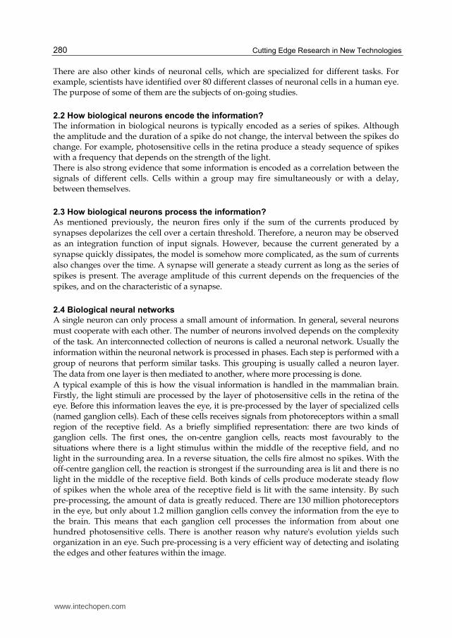
A typical example of this is how the visual information is handled in the mammalian brain. Firstly, the light stimuli are processed by the layer of photosensitive cells in the retina of the eye. Before this information leaves the eye, it is pre-processed by the layer of specialized cells (named ganglion cells). Each of these cells receives signals from photoreceptors within a small region of the receptive field. As a briefly simplified representation: there are two kinds of ganglion cells. The first ones, the on-centre ganglion cells, reacts most favourably to the situations where there is a light stimulus within the middle of the receptive field, and no light in the surrounding area. In a reverse situation, the cells fire almost no spikes. With the off-centre ganglion cell, the reaction is strongest if the surrounding area is lit and there is no light in the middle of the receptive field. Both kinds of cells produce moderate steady flow of spikes when the whole area of the receptive field is lit with the same intensity. By such pre-processing, the amount of data is greatly reduced. There are 130 million photoreceptors in the eye, but only about 1.2 million ganglion cells convey the information from the eye to the brain. This means that each ganglion cell processes the information from about one hundred photosensitive cells. There is another reason why nature's evolution yields such organization in an eye. Such pre-processing is a very efficient way of detecting and isolating the edges and other features within the image.

www.intechopen.com


281

The signals from both eyes are then combined within the called lateral geniculate nucleus or LNG, from where visual information travels to the visual cortex. The visual cortex is the largest part of cerebral cortex, which is a grey-matter of the brain. Here, in a series of regions, more complex features of visual input are recognized. For example, the first region is responsible for detecting lines of different lengths and different orientations. Later on, the combination of lines are recognized and processed. In the latest stages, the visual information is combined with the signals from other senses, and associated with the memory.

2.5 Learning within biological neural networks

The strengths of the synapses are flexible. On the long term, the amount of the

neurotransmitters released into the synaptic gap changes due to changes in neuronal

activities. By so-called Hebb's proposal (Hebb, 1946), which started the evolution of neural

networks, when an axon of one cell repeatedly excites another cell, the efficiency of the

synapse is increased. At the beginning, this idea was largely speculative. Later, however,

more and more biological evidence supports it (Fiete, 2003). Another basis for the learning

should be the changes in the dendrites themselves. A dendrite may grow and establish a

new connection with other cells. However, such growing of dendrites within an adult

animal's brain is not confirmed or is extremely rare. Some neuronal cells are interconnected

with each other directly. The learning process in this case is rather unclear.

3. Artificial neural networks

Digital computers are capable of performing millions of mathematical operations within a

very short amount of time. However, they are less successful at solving some problems,

which are effortlessly carried out by even the simplest biological systems. Development of

the first artificial neural networks began in the 1940s. It was motivated by the human desire

to understand the brain and to emulate some of its strengths (Fausett, 1994). The first ANNs

were very simple and had only a few neurons. In the 1980s, when the computers became

available to everyone, an enthusiasm for ANN was renewed. Different training strategies for

ANNs were developed and more complex problems solved. Advances in hardware over

recent years created a new renaissance. Using capable computers, it is now feasible to build

massive neural networks.

3.1 An artificial neuron

Several models exist for inner neuron behaviour that emulates the spiking nature of the

biological neuron (Gerstner & Werner, 2005). However, the representation of information

and the information processing within a biological neuron are very complex and the

implementations of those models can be very inefficient. As a consequence, in early artificial

neuronal networks, a simplified model of a neuron was used, as shown in Fig. 3.

Instead of using series of spikes, this model uses numerical quantities (either integer or

floating-point numbers). The magnitude of inputs and outputs corresponds to the frequency

of spikes within a real neuron. The values may be observed either continuously or at

discrete points in time.

A synapse is modelled by a multiplier with a constant. The input to the synapse is

multiplied by a weight that corresponds to different synaptic behaviour. Larger values of

the weights are associated with a large amount of neurotransmitters released, and vice-

www.intechopen.com


282

versa. The negative weights match the inhibitory synapses. The weights are set during the

training process of ANN, and usually remain fixed after that.

Fig. 3. Simplified model of an artificial neuron

Next, the weighted inputs are summarized by mimicking the integration function of the soma. In some neuron models, an additional correction factor or bias is also applied. After that, the sum is processed using the so-called activation function. This activation

function models the nonlinear characteristic of the action potential generation within the

biological neurons. The most common activation functions are the identity function (Eq. 1),

the step function (Eq. 2) and the sigmoid function (Eq. 3). The latter is frequently replaced

by the hyperbolic tangent function (Eq. 4), which is a good approximation of the sigmoid

function with =1.

( )i x x (1)

1,

( ) 0,

1,

x

x

x

x

(2)

1

( )1

x

x

eg x

e

(3)

( )x x

x x

e eh x

e e

(4)

The values of threshold and the steepness parameter are usually set accordingly to a specific problem. The represented functions (with the exception of identity) are a bipolar function with the output-value interval [-1, 1]. Unipolar versions of these functions are also common, some other output ranges may be used. The output value of an artificial neuron represents the axon within the biological neuron. The operation of an artificial neuron can be embodied within Eq. 5.

www.intechopen.com


283

1

( )n

i ij ij j jj

y f x w f x w

(5)

As seen from the equation, the weighted sum can be evaluated as the dot product between vector of the input values and vector of the corresponding synaptic weights. This can be done very efficiently using digital computers.

3.2 Topologies of the artificial neural networks

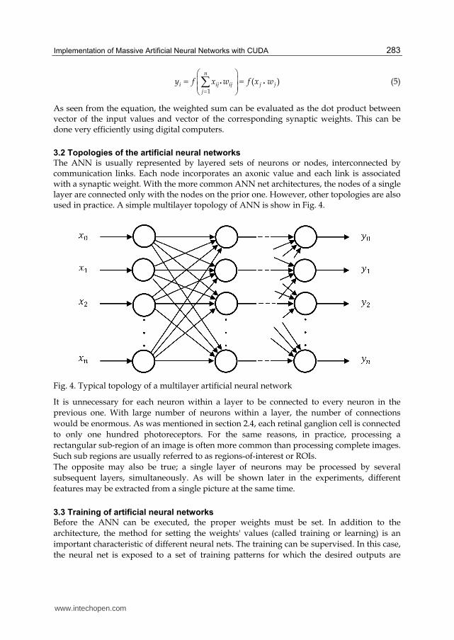
The ANN is usually represented by layered sets of neurons or nodes, interconnected by communication links. Each node incorporates an axonic value and each link is associated with a synaptic weight. With the more common ANN net architectures, the nodes of a single layer are connected only with the nodes on the prior one. However, other topologies are also used in practice. A simple multilayer topology of ANN is show in Fig. 4.

Fig. 4. Typical topology of a multilayer artificial neural network

It is unnecessary for each neuron within a layer to be connected to every neuron in the

previous one. With large number of neurons within a layer, the number of connections

would be enormous. As was mentioned in section 2.4, each retinal ganglion cell is connected

to only one hundred photoreceptors. For the same reasons, in practice, processing a

rectangular sub-region of an image is often more common than processing complete images.

Such sub regions are usually referred to as regions-of-interest or ROIs.

The opposite may also be true; a single layer of neurons may be processed by several

subsequent layers, simultaneously. As will be shown later in the experiments, different

features may be extracted from a single picture at the same time.

3.3 Training of artificial neural networks

Before the ANN can be executed, the proper weights must be set. In addition to the

architecture, the method for setting the weights' values (called training or learning) is an

important characteristic of different neural nets. The training can be supervised. In this case,

the neural net is exposed to a set of training patterns for which the desired outputs are

www.intechopen.com


284

known in advanced. The expected outputs are compared with the actual ones, and the

weights are adjusted accordingly to minimize any error. In unsupervised learning

algorithms, the weighs are adjusted without training patterns. The neural net is self-

adapting. In this case, the learning process tries to groups the input patterns into clusters

with similar intrinsic characteristics.

For a simple, single-layer networks, the learning algorithm is straightforward and can be

achieved mathematically. The most common algorithm for the training of multi-layer

artificial networks is the so-called back-propagation algorithm. This is the supervised

algorithm. For each training pattern, the difference (error) between the expected and actual

results is propagated back from the output layer to the input one. This process is repeated

until the error for each training pattern drops under a certain accepted level. The rate of

learning can be rather slow. For the back-propagation algorithms, the first derivative of the

activation function must be known. The detail description of back-propagation and other

multi-layer training algorithms can be found in (Fausett, 1994). In the experiments presented

in this work, the focus was on the ANN execution only.

In some cases, no extra training is required. The weighs for some neurons can be determined

from the nature of the neuron itself. For example, the retinal ganglion cell has a specific

functionality and the weight can be determined analytically. This will be demonstrated in

Fig. 17. The weights are adjusted in such a way that the output is most excitatory when a

proper combination of on-centre/off-centre light shines on the visual field of the neuron (the

output is +1). The opposite combination yield to the inhibitory response (the output is -1).

When the entire receptive field is illuminated with the same light intensity, no response is

generated (the output value is zero). With these rules and by considering the number of

"black" and "white" weights, the weight values can be calculated analytically.

I Iw 1 / 2 * N

E Ew 1 / 2 * N

The wI and wE represent the values of inhibitory end excitatory weights, respectively.

Similarly, the NI and NE corresponds to the number of these weights.

4. Implementation of artificial neural networks

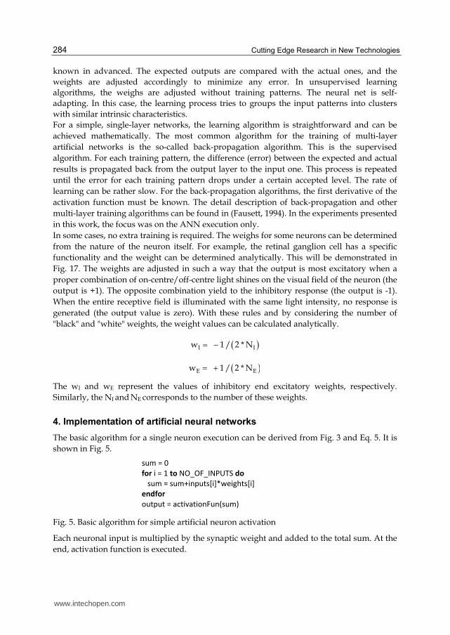
The basic algorithm for a single neuron execution can be derived from Fig. 3 and Eq. 5. It is

shown in Fig. 5.

Fig. 5. Basic algorithm for simple artificial neuron activation

Each neuronal input is multiplied by the synaptic weight and added to the total sum. At the

end, activation function is executed.

sum = 0

for i = 1 to NO_OF_INPUTS do

sum = sum+inputs[i]*weights[i]

endfor

output = activationFun(sum)

www.intechopen.com


285

In order to execute a layer of neurons, the same algorithm must be completed for each neuron. The execution of the ANN is usually performed in a layer-by-layer fashion. Firstly, the input nodes are processed, and the nodes from the first intermediate layer, etc. This is shown in Fig. 6.

Fig. 6. Elementary algorithm for ANN execution

The first layer is usually the input layer and contains the input data. Commonly, no processing is done in this layer. Similarly, the evaluated neurons in the last layer usually represent the outputs of a network. For a massive ANN, the neurons in a layer are typically organized within two or three-dimensional arrays. ANN can be implemented either in software or in hardware. The implementation with CUDA, which is the topic of a further section, can be observed as a hybrid between software and hardware implementation. A piece of software is executed several times on massively parallel multiprocessor architecture.

4.1 Software implementation

Most often, the ANN is implemented in software. The algorithms are simple enough for any computer language. In addition, there are numerous programming libraries and frameworks that simplify ANN construction. A very popular tool for ANN is the adaptive Neural Network Library included as an add-on in Matlab 5.3.1, and later. It is a collection of blocks that implement several Adaptive Neural Networks featuring different adaptation algorithms (Matlab, 2011). With this toll, only the simulation of a small ANNs is feasible. A good starting point for different software libraries and other resources for ANN can be found at (DMOZ, 2011). The main advantage of software implementation is that the programmer may utilize all resources of the computer. The application has access to large amount of memory, mass storages, input/output devices, etc. For example, the processing of visual data in real-time requires a direct connection to the camera; pictures may be loaded from a databases or a disk, etc. With other kinds of ANN implementation, this is not achieved that easily; usually the data must be prepared and send to the device where it will be processed. For massive ANNs, a large amount of storage is required to store values of weights and the

intermediate results of neurons. Nowadays, this is no longer an issue. Even modest personal

computers have enough computer memory for this. With other kinds of implementations,

the limited memory may present a problem.

In our experiments, dynamic memory regions organized as two-dimensional arrays were

used to represent the inputs, the weights and the intermediate values. The class definition of

such a memory region is presented in Fig. 7.

The data type determines the data domain of those values kept in the memory. This is usually a floating-point number, but can also be an integer or a byte. For convenience, regardless of the actual data type, the values are always processed as floats. The stride represents the actual data size of bytes on each data row. For some configurations, the data is aligned within the memory for more efficient access. There are also a number of routines (not shown in the code)

for i = 1 to NO_OF_LAYERS do

for j = 1 to NO_OF_NEURONS_IN_LAYER do

evaluateNeuron(i,j)

www.intechopen.com


286

that allow for direct loading or storing the data in several image formats. In this way, the data can be efficiently read from or write to several image formats from a disk or a memory stream.

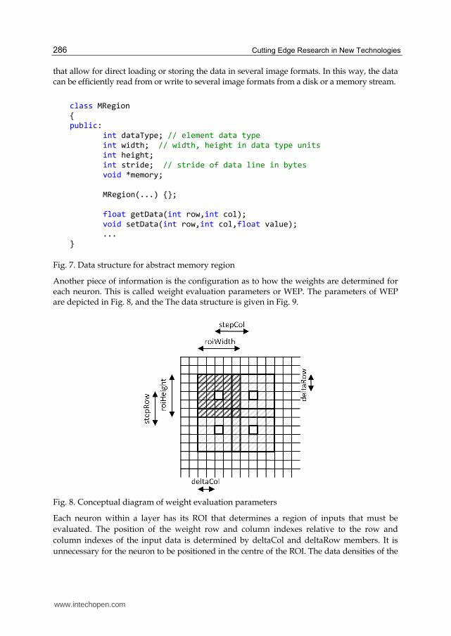
Fig. 7. Data structure for abstract memory region

Another piece of information is the configuration as to how the weights are determined for each neuron. This is called weight evaluation parameters or WEP. The parameters of WEP are depicted in Fig. 8, and the The data structure is given in Fig. 9.

Fig. 8. Conceptual diagram of weight evaluation parameters

Each neuron within a layer has its ROI that determines a region of inputs that must be

evaluated. The position of the weight row and column indexes relative to the row and

column indexes of the input data is determined by deltaCol and deltaRow members. It is

unnecessary for the neuron to be positioned in the centre of the ROI. The data densities of the

class MRegion

{

public:

int dataType; // element data type

int width; // width, height in data type units

int height;

int stride; // stride of data line in bytes

void *memory;

MRegion(...) {};

float getData(int row,int col);

void setData(int row,int col,float value);

...

}

www.intechopen.com


287

outputs are determined by the stepCol and stepRow parameters. As in the case of the ganglion

cells, the number of output neurons can be smaller than in the input layer. Two additional

Boolean flags determine the weight dependency. In general, each neuron in the layer can have

its own set of weights. In this case, the flag neuronDependent is set. In other cases, all the

neurons in a layer use the same set of weights. Sometimes a neuron from an output layer can

process the inputs from different input layers. In this case, the weights may be independent of

the input layer's index or not. For the later, the flag layerDependent is set.

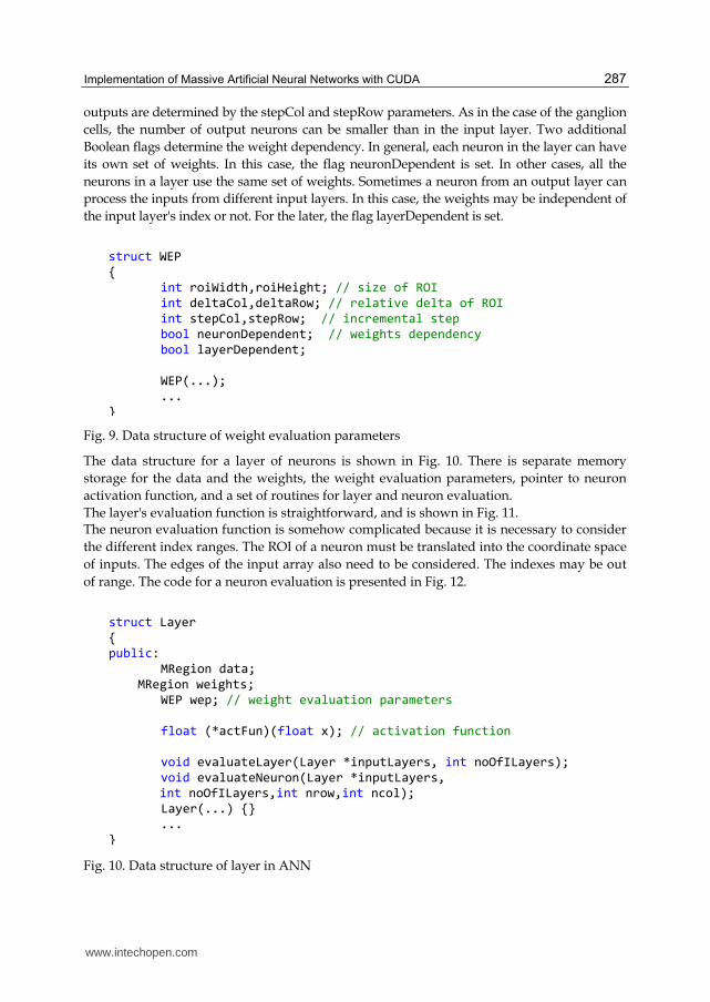
Fig. 9. Data structure of weight evaluation parameters

The data structure for a layer of neurons is shown in Fig. 10. There is separate memory

storage for the data and the weights, the weight evaluation parameters, pointer to neuron

activation function, and a set of routines for layer and neuron evaluation.

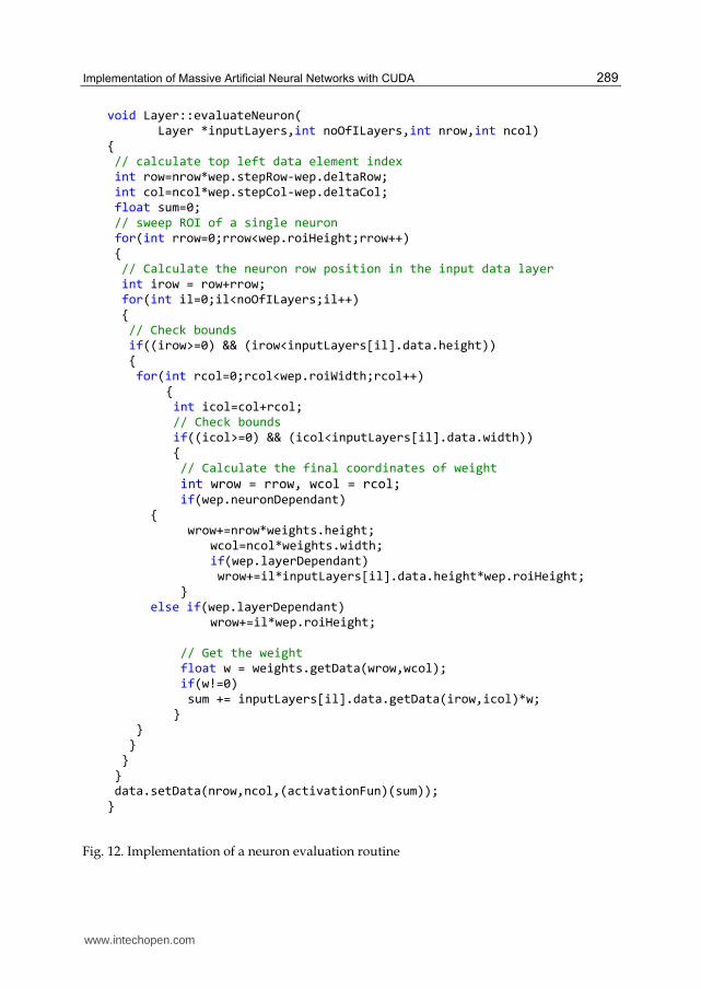
The layer's evaluation function is straightforward, and is shown in Fig. 11. The neuron evaluation function is somehow complicated because it is necessary to consider

the different index ranges. The ROI of a neuron must be translated into the coordinate space

of inputs. The edges of the input array also need to be considered. The indexes may be out

of range. The code for a neuron evaluation is presented in Fig. 12.

Fig. 10. Data structure of layer in ANN

struct WEP

{

int roiWidth,roiHeight; // size of ROI

int deltaCol,deltaRow; // relative delta of ROI

int stepCol,stepRow; // incremental step

bool neuronDependent; // weights dependency

bool layerDependent;

WEP(...);

...

}

struct Layer

{

public:

MRegion data;

MRegion weights;

WEP wep; // weight evaluation parameters

float (*actFun)(float x); // activation function

void evaluateLayer(Layer *inputLayers, int noOfILayers);

void evaluateNeuron(Layer *inputLayers,

int noOfILayers,int nrow,int ncol);

Layer(...) {}

...

}

www.intechopen.com


288

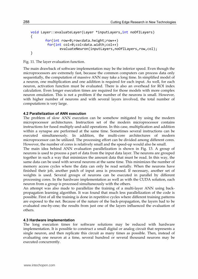
Fig. 11. The layer evaluation function.

The main drawback of software implementation may be the inferior speed. Even though the microprocessors are extremely fast, because the common computers can process data only sequentially, the computation of massive ANN may take a long time. In simplified model of a neuron, one multiplication and one addition is required for each input. As well, for each neuron, activation function must be evaluated. There is also an overhead for ROI index calculation. Even longer execution times are required for those models with more complex neuron emulation. This is not a problem if the number of the neurons is small. However, with higher number of neurons and with several layers involved, the total number of computations is very large.

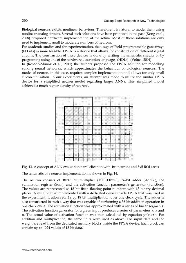
4.2 Parallelization of ANN execution The problem of slow ANN execution can be somehow mitigated by using the modern microprocessor architectures. Instruction set of the modern microprocessor contains instructions for fused multiply-and-add operations. In this case, multiplication and addition within a synapse are performed at the same time. Sometimes several instructions can be executed simultaneously. In addition, the multi-core architectures of modern microprocessor can be utilized. The processing effort can be divided among different cores. However, the number of cores is relatively small and the speed-up would also be small. The main idea behind ANN evaluation parallelization is shown in Fig. 13. A group of neurons is used to process a part of data from the input data layer. The neurons are grouped together in such a way that minimizes the amount data that must be read. In this way, the same data can be used with several neurons at the same time. This minimizes the number of memory access cycles where the data can only be read serially. When the neurons have finished their job, another patch of input area is processed. If necessary, another set of weights is used. Several groups of neurons can be executed in parallel by different processing cores. In the hardware implementation as well as with the CUDA solution, each neuron from a group is processed simultaneously with the others. An attempt was also made to parallelize the training of a multi-layer ANN using back-propagation learning algorithm. It was found that much less parallelization of the code is possible. First of all the training is done in repetitive cycles where different training patterns are exposed to the net. Because of the nature of the back-propagation, the layers had to be evaluated one-by-one; the results from just one of the layers influenced the evaluation of others.

4.3 Hardware implementation The long execution times for software solutions may be reduced with hardware implementation. It is possible to construct a small digital or analog circuit that represents a single neuron, and then replicate this circuit as many times as possible. Then, instead of evaluating one neuron at a time, several hundred or several thousand neurons may be executed concurrently.

void Layer::evaluateLayer(Layer *inputLayers,int noOfILayers) { for(int row=0;row<data.height;row++) for(int col=0;col<data.width;col++) evaluateNeuron(inputLayers,noOfILayers,row,col); }

www.intechopen.com


289

Fig. 12. Implementation of a neuron evaluation routine

void Layer::evaluateNeuron(

Layer *inputLayers,int noOfILayers,int nrow,int ncol)

{

// calculate top left data element index

int row=nrow*wep.stepRow-wep.deltaRow;

int col=ncol*wep.stepCol-wep.deltaCol;

float sum=0;

// sweep ROI of a single neuron

for(int rrow=0;rrow<wep.roiHeight;rrow++)

{

// Calculate the neuron row position in the input data layer

int irow = row+rrow;

for(int il=0;il<noOfILayers;il++)

{

// Check bounds

if((irow>=0) && (irow<inputLayers[il].data.height))

{

for(int rcol=0;rcol<wep.roiWidth;rcol++)

{

int icol=col+rcol;

// Check bounds

if((icol>=0) && (icol<inputLayers[il].data.width))

{

// Calculate the final coordinates of weight

int wrow = rrow, wcol = rcol; if(wep.neuronDependant)

{

wrow+=nrow*weights.height;

wcol=ncol*weights.width;

if(wep.layerDependant)

wrow+=il*inputLayers[il].data.height*wep.roiHeight;

}

else if(wep.layerDependant)

wrow+=il*wep.roiHeight;

// Get the weight

float w = weights.getData(wrow,wcol);

if(w!=0)

sum += inputLayers[il].data.getData(irow,icol)*w;

}

}

}

}

}

data.setData(nrow,ncol,(activationFun)(sum));

}

www.intechopen.com


290

Biological neurons exibits nonlinear behaviour. Therefore it is natural to model them using nonlinear analog circuits. Several such solutions have been proposed in the past (Kong et al., 2008) proposed hardware implementation of the retina. Most of these solutions are only used to implement small to moderate numbers of neurons. For academic studies and for experimentation, the usage of Field-programmable gate arrays (FPGAs) is more feasible. FPGA is a device that allows for construction of different digital circuits. The construction of these devices is done by writing the schematic circuits or by programing using one of the hardware description languages (HDLs). (Volnei, 2004) In (Rosado-Muñoz et al., 2011) the authors proposed the FPGA solution for modelling spiking neural networks, which approximates the behaviour of biological neurons. The model of neuron, in this case, requires complex implementation and allows for only small silicon utilization. In our experiments, an attempt was made to utilize the similar FPGA device for a simplified neuron model regarding larger ANNs. This simplified model achieved a much higher density of neurons.

Fig. 13. A concept of ANN evaluation parallelization with 4x4 neurons and 5x5 ROI areas

The schematic of a neuron implementation is shown in Fig. 14.

The neuron consists of 18x18 bit multiplier (MULT18x18), 36-bit adder (Add36), the summation register (Sum), and the activation function parameter’s generator (Function). The values are represented as 18 bit fixed floating-point numbers with 13 binary decimal places. A multiplier is implemented with a dedicated device inside FPGA that was used in the experiment. It allows for 18 by 18 bit multiplication over one clock cycle. The adder is also constructed in such a way that was capable of performing a 36-bit addition operation in one clock cycle. The activation function was approximated with a series of linear segments. The activation function generator for a given input produces a series of parameters k, x and n. The actual value of activation function was then calculated by equation y=k*x+n. For addition and multiplication, the same units were used as above. The input data and the weight are read from the dedicated memory blocks inside the FPGA device. Each block can contain up to 1024 values of 18-bit data.

www.intechopen.com


291

Fig. 14. Schematic of a neuron implemented within hardware

Although, they are extremely fast, there are several obstacles when using FPGA devices for ANN. Firstly, to process data, the inputs have to be provided by the main processor. In our case, the data was loaded into the external memory chip. The same is true as to when the results must be gathered. Secondly, the number of neurons that can be implemented inside FPA device is limited. In our device, 126 multipliers were available. Because of the limited memory available and because some multipliers were used for other purposes, it was only possible to implement 64 neurons. Massive ANN was implemented with the method described in the previous section. Another limiting factor is the amount of available internal memory inside a FPGA device. The weights for each neuron are stored in separate RAM block. The largest ROI available in this case was 32x32 input values. The number of RAM blocks limited. It was necessary to load a new data and weights after each execution cycle of 64 neurons. For this, data was transferred from external to internal memory, by means of software microprocessor implemented inside the device. This process prologues the execution of ANN. The ratio between the times of neuron execution and data transfer was around 1:20 for a typical case. In earlier experiments, an attempt was made to use the FPGA devices for the training of the

ANN. However, the amount of silicon consumption is doubled. In addition, because of the

increased memory requirements, only the training for a small ANNs could be implemented.

www.intechopen.com


292

5. Implementation of artificial neural networks with CUDA

Driven by demands from the mass consumer electronic market, the programmable Graphic

Processor Unit or GPU has evolved into device that largely outperforms any general Central

Processing Unit or CPU in both computational capabilities and memory bandwidth. GPUs are

capable to render high-definition 3D graphics in real-time. In order to do this, the GPU must

process millions and millions of pixels in every second. To achieve this, GPUs employ highly-

parallel architectures. At first, the process of graphic rendering was predefined and fixed

within hardware. Later, it was possible to write simple programs (called shaders) that define

how graphic is rendered. Soon after that, programmers tried to harness the great processing

power for solving non-graphical problems. This is known as General-Purpose Computing on

GPUs or GP-GPU. Instead of rendering a graphic on screen, specially designed shaders were

capable of doing the calculations and “rendering” the results into memory. Because of its

origin, the GPU was especially well-suited to address problems that could be expressed as

data-parallel computations – the same program being executed on many data elements, in

parallel. The drawback of this was that the programmers were forced to employ graphical

resources of GPUs and use graphical application programming libraries. In order to make

GPUs more universal, the manufacturers have changed the architectures of their newest

graphical devices, thus enabling them to be used for wider set of applications. Certain silicon

areas on GPUs are now devoted to facilitatingthe ease of parallel programming. These parts

are never used during picture rendering. The other elements are shared and can be used with

a graphical engine and for general parallel programming. GPU based devices now exists with

no video output. They are dedicated solely to parallel programming.

The practice of parallel programming is not something new, it has been in use for decades.

However, these programs run on large scale and expensive computers (see Herlihy &

Shavit, 2008). With recent evolution of GPUs, massive programming has become available

for everyone.

The execution of artificial neural networks or ANN is an intrinsically parallel problem;

hence, parallel computational architectures lead to a great improvement in speed. Because,

the researchers were start to use the GPUs from the very beginning, but what is new is that

the newest GPU architectures allow for a more general approach to ANN programming,

without taking into consideration the graphical aspects of GPUs.

5.1 CUDA

For the implementation of ANN with parallel programming, a Compute Unified Device

Architecture or CUDA was chosen (CUDA, 2011). CUDA is a general-purpose parallel

computing architecture developed by Nvidia GPU manufacturer. CUDA comes with a

software environment that allows developers to use C as a high-level programming

language. In CUDA terminology, the main unit of PC with general CPU is called the host

and the graphics card is called the device. The host and the device communicate with each

other through the high-speed bus. CUDA architecture allows several devices to be

connected to the same host. However, the programming management of several devices is

left to the programmer.

The basic unit of execution in CUDA is the so-called kernel. The kernel is a specially

marked C routine that may be invoked from the host. The kernel is executed in parallel

www.intechopen.com


293

multiple times by CUDA threads. The execution of several threads is grouped into larger

collections called thread blocks. For even greater parallelism, multiple tread blocks can be

run together in a grid. Although a kernel code is the same for all threads, each tread has its

own programming context (i.e. its own set of registers and local variables). In addition,

each tread in a thread block has its unique identification number called thread ID, and

each block in the grid has its unique block ID. The threads inside a block can be organized

into one-, two- or three-dimensional structures. This provides a natural way of

performing computation across the elements in those domains where data is presented in

a vector, matrix, or field form. Similarly, a block within a grid can be organized into one-

or two-dimensional structures.

The treads inside a block can communicate with each other by means of shared memory.

The shared memory is accessible from all threads within the same thread block. However,

the content of the memory is not preserved between executions of different blocks; the

content of the shared memory being undefined when the block starts its execution. The

access time of the shared memory in CUDA is the same as the access time of the registers.

This device has also a large amount of global memory (up to several GBytes). Its content has

the lifetime of an application. In contrast to the shared memory, the access time for the

global memory is at least 100 times slower. Therefore, if the same data is accessed several

times, it is feasible to copy it first from global memory to the shared one. Alternatively, the

data in the global memory can be organized as a texture memory. Textures are a part of

typical graphic applications for painting 2D images over 3D objects. In applications, the

texture memory provides a faster alternative to general memory because the texture

accesses are cached. The drawback is that the textures are read-only and require special

access functions. In the newest CUDA devices, access to the global memory is also cached.

There is also a small amount of the so-called constant memory. This read-only memory can

be set by the host. This memory is also cached and has a lifespan of the application.

Constant memory is ideal when using global application parameters.

CUDA provides synchronization between threads by means of barriers. When a thread

within a block reaches the barrier, it waits until all other threads reach the same point of

execution. CUDA also provides several atomic operations, which can solve possible race

conditions that may happen in parallel programs, where the same global variable is

modified by several threads simultaneously.

CUDA programs consist of intermixed code for both the host and for the CUDA device (files

with any CUDA code must have a .cu file extension). A special compiler (nvcc) pre-compiles

this code and splits it into the host and the device part. Both parts are then compiled

separately. Prior to execution, the compiled CUDA code is loaded into the device memory.

On a CUDA device, the threads are executed on a scalable array of multithreaded Streaming

Multiprocessors (SMs). Each SM consists of eight Scalar processors (SP) and some other

components. All SPs execute the same instruction at a time, and four successive clock cycles

are used to execute a single instruction for 32 threads. This is called a warp. Each SM has its

own shared memories and access to global, constant and texture memory. All threads in a

block are executed by the same SM. The threads are split into warps and executed

concurrently, according to the available resources, with hardware-based scheduler. The

context switch between warps is performed in zero-time.

www.intechopen.com


294

5.2 Representation of input and output data

During training and execution, the ANN usually reads the input data from disk or some

device (e.g. digital camera). The CUDA device has no direct access to these. Therefore, data

must be first loaded into the device. Currently, this can be done only by means of memory-

to-memory transfer between the host and the device. The same is true when the results must

be stored on the host. Although the transfer bandwidth can be very high, (e.g. with PCI

express 16x bus up to 8GB/sec) these transfers introduce a delay which may influence the

feasibility of using CUDA. In general, the transfer delay is only justifiable for large ANN.

For newer CUDA devices, it is possible to perform memory-to-memory transfer in parallel

with kernel execution: part of data space may be processed at the same time when the other

part is prepared. It is also possible to execute memory-to-memory transfer between two

CUDA devices without CPU involvement.

Very often, the data must be pre- and post-processed. Usually these operations can be

parallelized, so it can be done more efficiently on the device. For example, in image

processing, the picture is usually enhanced before a computation. This is usually well suited

for GPUs and parallel computation.

Natural data types for CUDA are integer and floating point values. Older CUDA devices

support only single precision floating-point numbers. This may be the problem if the

training algorithm relies on a greater accuracy and may impose some problems with the

convergence of some solutions. The newest generation of CUDA devices supports the

double-precision FP values. This is the standard for all future devices. However, with

double-precision arithmetic, the performance decreases. Because of GPU origins, the data on

CUDA devices may be very well organized into one, two or three-dimensional arrays.

Algebraic operations, such as vector and matrices multiplications, can be performed very

efficiently. There are several programming libraries available for CUDA that implements

optimized algebraic operations. The CUDA also supports pointers and, therefore, some sort

of dynamic data structures can be used. However, because of the single-instruction-

multiple-data nature of program executions, this may be inefficiently.

5.3 Representation of the weights

The weights of the ANN must also be transferred to the device memory. For most ANN

topologies, the weights are fixed after the training and remain the same during the

execution. For an older device, the best place to put them is in the read-only texture

memory. As mentioned before, this memory is cached and provides much greater

throughput. The mechanism of the cache is optimized for graphical applications and

produces the best results for 2D and 3D access patterns. This is well-suited for ANN

topologies where a neuron in some layer is connected to a small-clustered region of neurons

on a previous layer. For the new devices, this is not as clear because the main memory is

also caches. In most situations, some experimentation is required.

During the training and with ANN topologies where weigh changes continually during the

execution, the general global memory of CUDA devices must be used. Because of the large

latency, these algorithms that utilize the shared memory should be used. E.g., a multiprocessor

takes 4 clock cycles to issue one memory instruction for a warp. When accessing global

memory, there are between 400 to 600 clock cycles of memory latency. However, due to the

specifics of the CUDA device implementation, the global memory access by all threads of a

www.intechopen.com


295

warp can be coalesced into one or two memory transactions, if it satisfies some conditions (e.g.

each thread must access the memory in sequence, the accessed memory must be properly

aligned, etc.). The conditions depend on the version of the CUDA devices. Therefore, it is

difficult to implement a kernel routine that will be optimal for all boards.

5.4 Summarization of the neuron Inputs

As a part of the ANN execution, the input values of each neuron are multiplied by their

appropriate weights and then summarized, before the activation function is applied. This

operation is also frequently used in graphical applications and, therefore, GPUs may

perform it very efficiently by means of the so-called multiply-and-add (MAD) instruction.

The execution time for this instruction is only four clock cycles for single precision floating

point numbers.

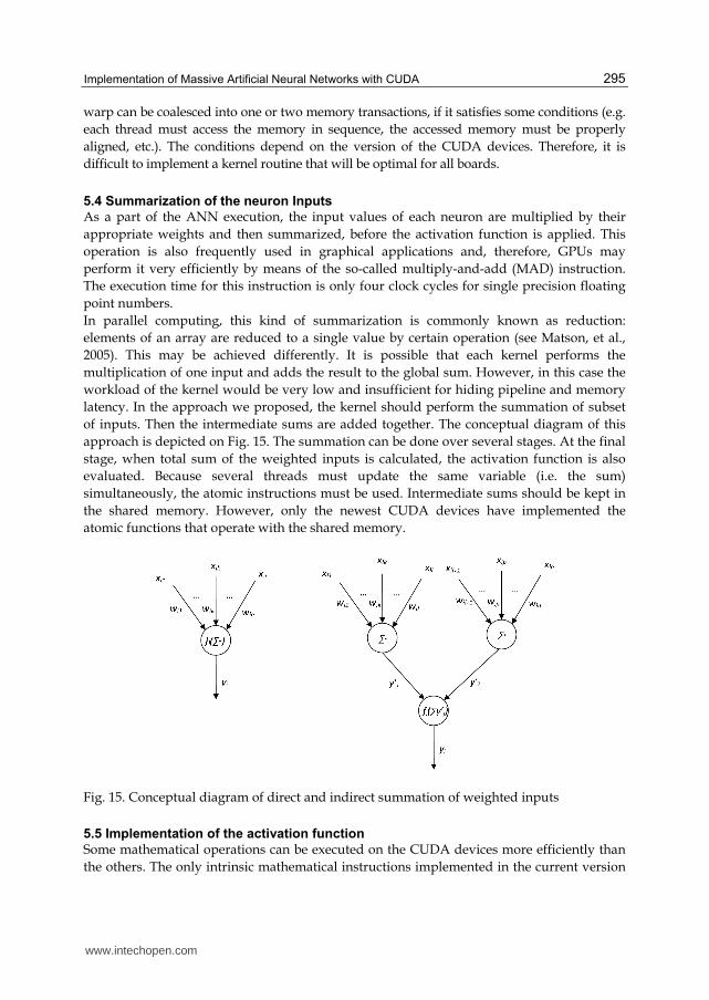
In parallel computing, this kind of summarization is commonly known as reduction:

elements of an array are reduced to a single value by certain operation (see Matson, et al.,

2005). This may be achieved differently. It is possible that each kernel performs the

multiplication of one input and adds the result to the global sum. However, in this case the

workload of the kernel would be very low and insufficient for hiding pipeline and memory

latency. In the approach we proposed, the kernel should perform the summation of subset

of inputs. Then the intermediate sums are added together. The conceptual diagram of this

approach is depicted on Fig. 15. The summation can be done over several stages. At the final

stage, when total sum of the weighted inputs is calculated, the activation function is also

evaluated. Because several threads must update the same variable (i.e. the sum)

simultaneously, the atomic instructions must be used. Intermediate sums should be kept in

the shared memory. However, only the newest CUDA devices have implemented the

atomic functions that operate with the shared memory.

Fig. 15. Conceptual diagram of direct and indirect summation of weighted inputs

5.5 Implementation of the activation function

Some mathematical operations can be executed on the CUDA devices more efficiently than

the others. The only intrinsic mathematical instructions implemented in the current version

www.intechopen.com


296

of CUDA devices are: reciprocal, square root, reciprocal of square root, sine, cosine, log, base

2, and exponential, base 2. In addition, some of these functions have limited accuracy. For

the implementation of more accurate version of these instructions and for other

mathematical functions, run-time routines are needed that consist of a sequence of

elementary operations. For example, there is no direct implementation of exponentiation of

base e, and must be implemented by other means. There does exists a primitive

implementation of natural exponential function (named __expf(x)), where the power of two

function is used (__expf(x)=__exp2f(x*LOG2_E)). This function can be implemented with a

sequence of simple instructions that take 32 clock cycles. However, this implementation

loses significant accuracy for large arguments. There is also a more accurate implementation

of this function (named expf(x)), which is much more expensive. Another example is the

single-precision floating-point division that takes 36 clock cycles. However, a primitive

function __fdividef(x, y) provides a faster version at 20 clock cycles. This function has the

same accuracy as the division. However, it produces the zero result for large values of y.

The “normal” division reduces the dividend and divisor by one quarter prior the operation

if the absolute value of y is too big. Integer division and modulo operation are particularly

costly and should be avoided if possible, or replaced by bitwise operations.

The identity and the step activation functions are simple to implement. On the other hand,

the sigmoid and the hyperbolic tangent functions are the composite of several basic

operations. A big reduction of execution time may be achieved in some situations if a less

accurate version of those operations can be used. For example, the activation function is

very often implemented by the hyperbolic tangent function and, if accuracy is not a

problem, then a code can be used:

y = __fdividef(__expf(x)-1/__expf(x),__expf(x)+1/__expf(x));

The equation is optimized by the compiler to a single call of the exponentiation function, one call of the reciprocal function, one addition, one subtraction and one division. The reciprocal takes 16 clock cycles, the addition and subtraction take four clock cycles each. Therefore, the exaction time of this activation function can be 76 clock cycles. The more accurate implementation of hyperbolic function would take at least three times more clock cycles.

5.6 Training and execution of ANN

The training and execution of ANN is performed in three steps: preparation of the initial

data, transfer of the data to the CUDA device, evocation of the kernel routine, and transfer

of the result to the host. The same data may be evaluated using several kernels sequentially

and data transfer operations may overlap with the kernel execution. It is also feasible to

distribute the workload between several CUDA devices. The upper-end graphical cards

incorporate two GPUs, which can be used as two independent CUDA devices. There are

dedicated CUDA devices with no graphical output, and with up to 256 processing cores.

6. Experiments

A set of experiments was performed, in order to augment the theoretical research. An attempt was made to implement a massive ANN with software, with hardware and with the

www.intechopen.com


297

CUDA framework. The first experiment tried to implement a neocognitron. This is an ANN designed to recognize written text (Fukushima et al., 1983). The description of neocognitron presented in the (Fausett, 1994) was used. The idea behind the neocognitron is to mimic the video processing path found in humans and other animals, as described in section 2.4. The data is processed in stages. During the first stage, the basic elements are extracted from input pictures. The basic elements are short lines with different orientations. Several layers of network are trained to respond to these features. At the latter stages, a combination of basic features is processed. Finally, specific characters are recognized. In this specific case, the ANN consisted of 9 layers of neurons. Most layers are further divided into sub-layers, which provide around 160 grouping of neurons. The total number of neurons is around 14 thousand with approximately 160 thousand synapses. The inputs are simple patterns of size 19x19 monochrome pixels. The output is a vector of bits, each corresponding to a specific character (in our case, it was one of the ten decimal digits). The ANN is capable to recognize one character at the time. It cannot be claimed that this is the best ANN for handwritten character recognition. However, it is complex enough to test and compare different implementations. The training of ANN was implemented in software. During software implementation, the code described in section 4.1 was used. All neurons in

a single layer were processed at the same time. The tests were executed on a Xeon processor

(W5590 running at 3.33 GHz).

For the hardware implementation, the FPGA solution presented in the section of 4.3 was

used. The FPGA device was Xilinx Spartan3A XC3SD3400A, running at 25 MHz (Xilinx,

2011). An extra memory chip with capacity of 4 Mbytes was connected to the device. Within

the FPGA, a soft-processor Picoblaze was used to move the data between external an

internal memory. The device was connected to the PC via serial communication link.

Fig. 16. The source code excerpt of a kernel for a neuron evaluation

The matrix of 8x8 neurons was used. All necessary data and configuration parameters were put into the external memory, prior the execution. With each execution cycle of ANN, a new set of data and parameters was loaded into the device. For the implementation with CUDA framework, a slightly modified version of the code was used. In compiler for CUDA, the support for classes is somehow limited. At this time, the CUDA does not support the virtual functions. Similarly, the pointers to the functions are yet unsupported. The kernel routine for the neuron evaluation is shown in Fig. 16.

__global__ void

evaluateNeuron(Layer *me, Layer *inputLayers,int noOfILayers)

{

// calculate actual coordinates of a neuron

const unsigned int nrow = blockDim.y*blockIdx.y+threadIdx.y;

const unsigned int ncol = blockDim.x*blockIdx.x+threadIdx.x;

// access number of threads in this block

const unsigned int num_threads = blockDim.x;

...

me->data.setData(nrow,ncol,activationFun(sum));

}

www.intechopen.com


298

The class method was converted to the standard C routine. Additional parameter was

added that represents the reference to a current layer. All the neurons in a layer are executed

at the same time. This eliminates the loop presented in Fig. 11. The indexes of a neuron are

determined by block and thread IDs.

For layer-by-layer execution of the ANN as a whole, the kernel was executed several times

with different parameters. All the data and parameters were put into the GPU memory prior

to the execution.

Firstly, the experiments were implemented with the dedicated CUDA device with compute

capability 1.3 (Tesla C1060). Recently, a high-end gamming card has been acquired with the

compute capability 2.0 (GeForce GTX595). The level of parallelization in latter device is much

higher. The new architecture incorporates global memory cache and it is possible to use two

different configuration of shared memory (16KB or 48KB instead of only the 16KB in previous

versions). With older devices, each thread block can contain maximum of 512 threads. In our

case, this is also the maximum number of neurons per block. Prior the evaluation of the

neurons, the inputs could be copied from the global to the shared memory. However, the

number of inputs is limited by the maximum amount of shared memory per block. With 16KB

of shared memory, 1024 synapses can be implemented. This corresponds to a grid with 32x32

inputs. Nevertheless, the shared memory is also used to store intermediate results during the

layer evaluation. At least as much values as there are neurons in a block are needed. At

maximum, the number of inputs that may be put into the shared memory is halved. With

newer devices and with 48KB of shared memory per block, intermediate values for all 1024

neurons plus another 2048 values for the inputs can be maintained.

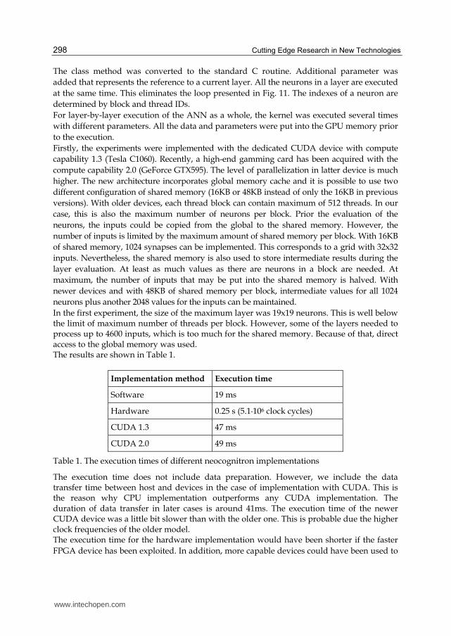
In the first experiment, the size of the maximum layer was 19x19 neurons. This is well below the limit of maximum number of threads per block. However, some of the layers needed to process up to 4600 inputs, which is too much for the shared memory. Because of that, direct access to the global memory was used. The results are shown in Table 1.

Implementation method Execution time

Software 19 ms

Hardware 0.25 s (5.1·106 clock cycles)

CUDA 1.3 47 ms

CUDA 2.0 49 ms

Table 1. The execution times of different neocognitron implementations

The execution time does not include data preparation. However, we include the data transfer time between host and devices in the case of implementation with CUDA. This is the reason why CPU implementation outperforms any CUDA implementation. The duration of data transfer in later cases is around 41ms. The execution time of the newer CUDA device was a little bit slower than with the older one. This is probable due the higher clock frequencies of the older model. The execution time for the hardware implementation would have been shorter if the faster

FPGA device has been exploited. In addition, more capable devices could have been used to

www.intechopen.com


299

implement larger number of neurons. For example, the Vitrex-7 family of FPGA devices

contain up-to 3600 multipliers and as much as that number of neurons can be implemented.

Each multiplier is capable of operating at 638 MHz.

There is enough room for additional optimization for both software and CUDA

implementation. Instead of the general neuron evaluation routine, a specialized one can be

used for each of the different layer configurations. In this way, some loops can be unfolded

and some expressions simplified. We have not tried to utilize several processing cores, as

yet. Similarly, with several CUDA devices, it would be possible to divide the job into parts

and process them simultaneously.

A higher difference was expected between the results of software and CUDA

implementation. High-end CPU was used and the number of neurons was too small for

significant difference. Because of that, another experiment with much larger number of

neurons was conducted.

Fig. 17. Weights for off-centre and on-centre ganglion cell simulation

Fig. 18. The original image and the result of the second experiment

In the second experiment, an early stage of visual processing in the retina was implemented.

The off-centre/on-centre ganglion cells were realized in the manner described in section 2.4.

High-definition photography was taken as an input. The size of the input grid is 5616x3744

pixels. The output grid of neurons is reduced to one third. The ROI of each neuron is 31x31

www.intechopen.com


300

pixels. The weights were set in advance to mimic the processing of the ganglion cells. A

biological ganglion cell has approximately circular ROI. For simplicity, we used the

rectangular patterns shown on Fig. 17. The white areas represent the excitatory synapses;

the black areas correspond to the inhibitory synapses. The sum of weights is exactly zero.

This mimic the ganglion cells response in the diffuse light. The weights pattern is combined

with the threshold activation function to get monochromatic (black and white) result. The

original and processed picture with off-centre weights is shown on Fig. 18. The result

illustrates how edge detection is processed in the human eye.

The results of the second experiment are shown in Table 2.

Implementation method Execution time

Software 224 s

Hardware -

CUDA 1.3 670 ms

CUDA 2.0 799 ms

Table 2. The execution times of the second experiment

The amount of data was too high for the hardware implementation. The execution time of

the software version was three orders of magnitude slower than the CUDA implementation.

The data transfer between the host and the GPU device contributed to about 80% of total

execution time.

7. Conclusion

Today, advances in hardware allow the ANN programmers to have efficient

implementations of massive neural networks that operate in real-time. For the small ANN

topologies, the presented approach is not feasible. It is possible to run several ANN in

parallel on a single or several devices. For example, in the case of character recognition,

different characters may be evaluated simultaneously.

From all currently available parallel programming environments, CUDA is most suitable for

ANN because it is the most mature, and can be used with wide range of products. However,

the solution with CUDA is not ideal. The CUDA is bound to a single manufacturer and

cannot be used with graphical cards of the others. The CUDA devices are still evolving.

Each new generation introduces some new features that make general parallel

programming more consistent and easier. At the same time, the optimization approach used

with one device's generation may be obsolete or inefficient with another.

Another consideration is the amount of time needed to put the input data into the CUDA

device and to get the results. As was shown during the experiments, this can take longer

than the processing alone. However, this also means that more complex problems can be

solved within approximately the same time.

In the current experiments, we neglected the study of training algorithms for the multilayer

neural networks. The main reason is that the training algorithms are very difficult to be

www.intechopen.com


301

parallelized. The presumption was that the weights would be calculated only once.

However, there are ANN topologies where training is executed continuously and must be

included in the final implementation.

In the future, we will try to implement other neuronal models for comparison if one model is better than another or if one model allows for solving larger classes of problems than the others.

8. References

BBP (2011). Home page of the Blue Brain Project. Available at http://bluebrain.epfl.ch/

CUDA(2011).Cuda Developers Page, Available from

http://developer.nvidia.com/category/zone/cuda-zone

Dayan, P. & Abbot L.F. (2001) Theoretical Neuroscience: Computational and Mathematical

Modeling of Neural Systems. MIT Press, Cambridge. ISBN 0-262-04199-5

DMOZ (2011). Portal to different ANN resources. Available at

http://www.dmoz.org/Computers/Artificial_Intelligence/Neural_Networks/

Fausett, L. (1994). Fundamentals of Neural Networks: architectures, algorithms, and application.

Prentice Hall, New Jersey.

Fiete, I. R. (2003) Learning and coding in biological neural networks. PhD thesis. Harvard

University, Cambridge, Massachusetts.

Fukushima K., Miyake S. & Ito T. (1983) Neocognitron: a neural network model for a

mechanism of visual pattern recognition. IEEE Transactions on Systems, Man, and

Cybernetics, Vol. 13, 826–834.

Gerstner, W. & Werner, M.K. (2005). Spiking Neuron Models, Single Neurons, Population,

Plasticity, Cambridge University Press, Cambridge, UK

Hebb, D. O. (1946), Organization of Behavior: A Neuropsychological Theory (Wiley, Inc.,

ADDRESS, 1949).

Herlihy, M. & Shavit, N. (2008) The Art of Multiprocessor Programming. Elsevier,

Burlington.

Kong, J., Sung, D., Hyun, H. & Shin, J. (2008) A 160×120 Edge Detection Vision Chip for

Neuromorphic Systems Using Logarithmic Active Pixel Sensor with Low Power

Dissipation. In: Lecture Notes in Computer Science. Springer, Berlin, ISBN: 978-3-540-

69159-4, pp: 97-106.

Matlab (2011). Matlab ANN Package, Available at

http://www.mathworks.com/matlabcentral/fileexchange/976-ann

Matson, T.G., Sanders, B.A. & Massingill, B.L. (2005) Patterns for Parallel Programming.

Pearson Education, Boston

Nicholls, J. G., Martin A. R., Wallace B. G. & Fuchs, P. A. (2001) From Neuron to Brain: A

Cellular and Molecular Approach to the Function of the Nervous System. Sinauer

Associates, 4th ed. ISBN: 0878934391

Rosado-Muñoz, A., Fijałkowski, A.B., Bataller-Mompeán, M. & Guerrero-Martínez J. (2011).

FPGA implementation of Spiking Neural Networks supported by a Software

Design Environment. Proceedings of 18th IFAC World Congress, Milano, Italy.

Volnei, A. P. (2004) Circuit Design with VHDL. MIT Press. Cambridge. ISBN: 0-262-16224-5

Xilinx (2011). Home page of Sparatn 3a FPGA devices. Available at

www.intechopen.com


302

http://www.xilinx.com/products/spartan3a/index.htm

www.intechopen.com

Cutting Edge Research in New TechnologiesEdited by Prof. Constantin Volosencu

ISBN 978-953-51-0463-6Hard cover, 346 pagesPublisher InTechPublished online 05, April, 2012Published in print edition April, 2012

InTech EuropeUniversity Campus STeP Ri Slavka Krautzeka 83/A 51000 Rijeka, Croatia Phone: +385 (51) 770 447 Fax: +385 (51) 686 166www.intechopen.com

InTech ChinaUnit 405, Office Block, Hotel Equatorial Shanghai No.65, Yan An Road (West), Shanghai, 200040, China

Phone: +86-21-62489820 Fax: +86-21-62489821

The book "Cutting Edge Research in New Technologies" presents the contributions of some researchers inmodern fields of technology, serving as a valuable tool for scientists, researchers, graduate students andprofessionals. The focus is on several aspects of designing and manufacturing, examining complex technicalproducts and some aspects of the development and use of industrial and service automation. The bookcovered some topics as it follows: manufacturing, machining, textile industry, CAD/CAM/CAE systems,electronic circuits, control and automation, electric drives, artificial intelligence, fuzzy logic, vision systems,neural networks, intelligent systems, wireless sensor networks, environmental technology, logistic services,transportation, intelligent security, multimedia, modeling, simulation, video techniques, water plant technology,globalization and technology. This collection of articles offers information which responds to the general goal oftechnology - how to develop manufacturing systems, methods, algorithms, how to use devices, equipments,machines or tools in order to increase the quality of the products, the human comfort or security.

How to referenceIn order to correctly reference this scholarly work, feel free to copy and paste the following:

Domen Verber (2012). Implementation of Massive Artificial Neural Networks with CUDA, Cutting EdgeResearch in New Technologies, Prof. Constantin Volosencu (Ed.), ISBN: 978-953-51-0463-6, InTech,Available from: http://www.intechopen.com/books/cutting-edge-research-in-new-technologies/implementation-of-massive-artificial-neural-networks-with-cuda

© 2012 The Author(s). Licensee IntechOpen. This is an open access articledistributed under the terms of the Creative Commons Attribution 3.0License, which permits unrestricted use, distribution, and reproduction inany medium, provided the original work is properly cited.

http://creativecommons.org/licenses/by/3.0

implementation of massive artificial neural networks with cuda

Documents