implementation considerations for fpga ... considerations for fpga-based adaptive transversal filter...
TRANSCRIPT

IMPLEMENTATION CONSIDERATIONS FOR FPGA-BASED ADAPTIVE
TRANSVERSAL FILTER DESIGNS
By
ANDREW Y. LIN
A THESIS PRESENTED TO THE GRADUATE SCHOOL OF THE UNIVERSITY OF FLORIDA IN PARTIAL FULFILLMENT
OF THE REQUIREMENTS FOR THE DEGREE OF MASTER OF ENGINEERING
UNIVERSITY OF FLORIDA
2003

Copyright 2003
by
Andrew Y. Lin

ACKNOWLEDGMENTS
I would like to thank my advisory committee members, Dr. Jose Principe, Dr. Karl
Gugel and Dr. John Harris, for their guidance, advice, and encouragement toward
successful completion of this project.
I also thank my fellow Applied Digital Design Laboratory members, Scott
Morrison, Jeremy Parks, Shalom Darmanjian and Joel Fuster, for their unconditional help
of my research everyway they can.
My special thanks go to my parents, who have been supportive and caring
throughout every step of my life, including my graduate years at University of Florida.
Altera Corp. has provided software and hardware in support of my thesis.
iii

TABLE OF CONTENTS Page ACKNOWLEDGMENTS ................................................................................................. iii
LIST OF FIGURES .......................................................................................................... vii
ABSTRACT....................................................................................................................... ix
CHAPTER 1 INTRODUCTION ........................................................................................................1
1.1 Problem Statement..................................................................................................1 1.2 Tradeoffs in Choosing Fixed-point Representation................................................3 1.3 Motivation and Outline of the Thesis .....................................................................5
2 THEORETICAL BACKGROUND ON LINEAR ADAPTIVE ALGORITHMS.......7
2.1 Discrete Stochastic Processes .................................................................................7 2.1.1 Autocorrelation Function..............................................................................7 2.1.2 Correlation Matrix ........................................................................................8 2.1.3 Yule-Walker Equation..................................................................................9 2.1.4 Wiener Filters .............................................................................................10
2.2 Method of Steepest Descent .................................................................................12 2.2.1 Steepest Descent Algorithm .......................................................................12 2.2.2 Wiener Filters with Steepest Descent Algorithm .......................................13
2.3 Least Mean Square Algorithm..............................................................................14 2.3.1 Overview ....................................................................................................14 2.3.2 The Algorithm ............................................................................................15 2.3.3 Applications................................................................................................16
2.3.3.1 Adaptive noise cancellation .............................................................16 2.3.3.2 Adaptive line enhancement ..............................................................17
3 FINITE PRECISION EFFECTS ON ADAPTIVE ALGORITHMS .........................18
3.1 Quantization Effects .............................................................................................19 3.1.1 Rounding ....................................................................................................19 3.1.2 Truncation...................................................................................................21 3.1.3 Rounding vs. Truncation ............................................................................22
3.2 Input Quantization Effects....................................................................................23 3.3 Arithmetic Rounding Effects ................................................................................24
iv

3.3.1 Product Rounding Effects...........................................................................25 3.3.2 Coefficient Rounding Effects .....................................................................26 3.3.3 Slowdown and Stalling...............................................................................27 3.3.4 Saturation....................................................................................................29 3.3.5 Solutions for Arithmetic Quantization Effects ...........................................31
3.4 Simulation Result..................................................................................................31 3.4.1 Rounding vs. Truncation ............................................................................32 3.4.2 Effects of Product Rounding at the Convolution Stage..............................33 3.4.3 Effects of Product Rounding at the Adaptation Stage................................35 3.4.4 Clamping Technique ..................................................................................36 3.4.5 Sign Algorithm ...........................................................................................38
3.5 Remarks ................................................................................................................39 4 SOFTWARE SIMULATION OF A FIXED-POINT-BASED POWER-OF-TWO
ADAPTIVE NOISE CANCELLER...........................................................................40
4.1 Modular Overview................................................................................................41 4.2 Data Quantization .................................................................................................42 4.3 Simulation Results ................................................................................................43
5 HARDWARE IMPLEMENTATION OF AN INTEGER-BASED POWER OF TWO
ADAPTIVE NOISE CANCELLER IN STRATIX DEVICES..................................45
5.1 Stratix Devices......................................................................................................46 5.1.1 Device Architecture....................................................................................46 5.1.2 Embedded DSP Blocks...............................................................................47
5.2 Design Specifications ...........................................................................................48 5.2.1 Structural Overview....................................................................................48 5.2.2 The Power-of-Two Scheme........................................................................49 5.2.3 Data Flow and Quantization.......................................................................50
5.3 Dynamic Component Instantiation in VHDL.......................................................50 5.4 Simulation and Implementation Results...............................................................52 5.5 Performance Comparison of Stratix and Traditional FPGAs ...............................53
5.5.1 Speed ..........................................................................................................54 5.5.2 Area ............................................................................................................54
5.6 Pipelining..............................................................................................................55 5.6.1 Optimal Multiplier Pipeline Stages ............................................................57 5.6.2. Optimal Adder-chain Pipeline Stages .......................................................58 5.6.3 Tradeoffs in Introducing Latency into Adaptive Systems..........................60 5.6.4 Performance of the Pipelined Adaptive System.........................................63
5.7 Performance Comparison of FPGAs and DSP Processors ...................................65 5.7.1 Speed ..........................................................................................................66 5.7.2 Power Consumption ...................................................................................67
6 CONCLUSION AND FUTURE WORK ...................................................................69
6.1 Conclusion ............................................................................................................69
v

6.2 Future Work..........................................................................................................71 APPENDIX A MATLAB SCRIPTS...................................................................................................73
B VHDL CODES ...........................................................................................................78
LIST OF REFERENCES...................................................................................................90
BIOGRAPHICAL SKETCH .............................................................................................93
vi

LIST OF FIGURES
Figure page 1-1. Conventional Adaptive Filter Configuration...............................................................2
1-2. Two Options of Quantization ......................................................................................4
2-1. Block diagram of a Statistical Filtering Problem. ......................................................11
2-2. Block Diagram of an Adaptive FIR Filter .................................................................13
2-3. Adaptive Noise Cancellation Block Diagram ...........................................................17
2-4. Adaptive Line Enhancer Block Diagram...................................................................17
3-1. Rounding Effects ........................................................................................................20
3-2. Truncation Effects ......................................................................................................21
3-3. MAC Unit Block Diagram ........................................................................................25
3-4. System Identification Block Diagram .......................................................................32
3-5. Experimental Setup for Rounding vs. Truncation .....................................................32
3-6. Simulation Result for Rounding vs. Truncation........................................................33
3-7. Additional Quantizers at the Convolution Stage .......................................................34
3-8. Effects of Product Quantization at the Convolution Stage........................................34
3-9. Additional Quantizers at the Adaptation Stage .........................................................35
3-10. Effects of Product Quantization at the Convolution and Adaptation Stages............36
3-11. Tap weight Track for Clamping Technique ............................................................37
3-12. Misadjustment Plot for Clamping Technique..........................................................38
3-13. Misadjustment for Sign Algorithm vs. LMS...........................................................39
4-1. Adaptive Noise Canceller Block Diagram .................................................................41
vii

4-2. Internal Structure of the Noise Canceller with Quantizers.........................................42
4-3. Weight Tracks for Fixed-point Systems....................................................................43
4-4. Misadjustment Plots of Fixed-point Systems and a Floating-point System..............44
5-1. Stratix Device Block Diagram....................................................................................47
5-2. Embedded DSP Block Diagram .................................................................................48
5-3. Adaptive Transversal Filter Block Diagram..............................................................49
5-4. Waveform Simulation Result of the Adaptive Noise Canceller................................52
5-5. Logic State Analyzer Result of the Adaptive Noise Canceller .................................53
5-6. Plot of Filter Order vs. Speed ....................................................................................54
5-7. Plot of Filter Order vs. Area .......................................................................................55
5-8. Pipelined Multiplier Test Module..............................................................................57
5-9. Maximum Data Rate of three Multipliers with Various Pipeline Stages ..................58
5-10. Adder-chain Test Module........................................................................................59
5-11. Adder-chain Data Rate with Respect to Number of Adders ....................................59
5-12. Pipelined and Buffered Adaptive System Block Diagram .......................................60
5-13. Time-aligned Adaptive System Block Diagram.......................................................63
5-14. Pipelined Adaptive System Performance .................................................................64
5-15. Power Consumption Plot for Various Devices........................................................67
viii

Abstract of Thesis Presented to the Graduate School
of the University of Florida in Partial Fulfillment of the Requirements for the Degree of Master of Engineering
IMPLEMENTATION CONSIDERATIONS FOR FPGA-BASED ADAPTIVE TRANSVERSAL FILTER DESIGNS
By
Andrew Y. Lin
August, 2003
Chair: José C. Príncipe Major Department: Electrical and Computer Engineering
Adaptive filters have become vastly popular in the area of digital signal processing.
However, adaptive filtering algorithms assume infinite-precision whereas in reality,
digital hardware is of finite-precision. The effects of finite-precision on adaptive
algorithms are studied in this thesis and techniques rendering these effects are presented.
Simulation results are also presented to verify the techniques targeting specifically to the
Least Mean Square (LMS) algorithm. Finally, a fixed-point-based adaptive transversal
filter is simulated in a new family of FPGA devices with embedded DSP blocks. The
cost-benefit and tradeoff of pipelining are studied. The performance of this new family
of FPGA devices is compared against DSP processors, as well as traditional FPGA
devices that do not have embedded DSP blocks.
ix

CHAPTER 1 INTRODUCTION
1.1 Problem Statement
Significant contributions have been made in the past thirty years in the signal
processing field. Particularly digital signal processing (DSP) systems have become
attractive due to the advances in digital circuit design and the systems’ reliability,
accuracy and flexibility. One of the DSP applications is called filtering, where the digital
system’s objective is to process a signal in order to manipulate the information contained
in the input signal. As described in DiCarlo [7], a filter is a device that maps its input
signal to another output signal facilitating the extraction of the desired information
contained in the input signal. For a time-invariant filter, the internal parameters and the
structure of the filter are fixed. Once specifications are given, the filter’s transfer
function and the structure defining the algorithm are fixed.
An adaptive filter is time-varying since their parameters are continually changing in
order to meet certain performance requirement. Usually the definition of the
performance criterion requires the existence of a reference signal, which is absent in
time-invariant filters. The general set up of an adaptive filtering environment is
illustrated in Figure 1-1, where n is the iteration index, x(n) denotes the input signal, y(n)
is the adaptive filter’s output signal, and d(n) defines the reference or desired signal. The
error signal e(n) is the difference between the desired d(n) and filter output y(n). The
error signal is used as a feedback to the adaptation algorithm in order to determine the
appropriate updating of the filter’s coefficients, or tap weights. The minimization
1

2
objective is for the adaptive filter’s output signal matching the desired signal in some
sense.
Figure 1-1. Conventional Adaptive Filter Configuration
The minimization objective can be viewed as a function of the input, desired, and output
signals, or consequently a function of the error signal. One of the most commonly used
objectives is to minimize the mean square error, that is, the objective function is defined
as
)]([)]([ 2 neEneF = . (1.1)
Adaptive filters can be implemented either in Finite Impulse Response (FIR) form
or in Infinite Impulse Response (IIR) form. FIR filters are usually implemented in non-
recursive structures, whereas IIR filters employ recursive realizations. In the case of FIR
realizations, the most widely used adaptive filter structure is the transversal filter, also
known as tapped delay line structure.
As will be derived in Chapter 2, all adaptive algorithms including the Least Mean
Square (LMS) algorithm for example, assume infinite precision. In other words, there is
infinite storage for information needed to perform adaptation. However, it is not the case
3
in reality, where computers or digital hardware which implement adaptive algorithms all
contain limited storage for information, that is, numbers are stored in finite precisions.
Due to finite precisions in digital hardware, quantization must be performed in
either or all of the following areas:
• Input and reference signals;
• Product quantization in convolution stage;
• Coefficient quantization in adaptation stage.
Quantization noise is introduced in all of the above areas. The effects of quantization are
discussed in this thesis.
DSP applications including adaptive systems have traditionally been implemented
with either fixed-point or floating-point microprocessors. However, with its growing die
size as well as incorporating the embedded DSP block, the FPGA devices have become a
serious contender in the signal processing market. Although it is not yet feasible to use
floating-point arithmetic in modern FPGAs, it is sufficient to use fixed-point arithmetic
and still achieve tap-weight convergence for adaptive filters. This thesis also investigates
the performance among FGPAs and DSP processors in terms of speed and power
consumption.
1.2 Tradeoffs in Choosing Fixed-point Representation
Since infinite precision is not available in the real world, tradeoffs must be made in
implementation of adaptive systems in finite precision. By increasing the wordlength, a
system can increase the data precision in which it can represent. However, the amount of
hardware also increases, and that leads to larger circuitry and slower system speed. If
wordlength is insufficient, saturation or stalling may occur due to the inadequacy of data

4
storage, even though smaller wordlength reduces amount of hardware. Therefore, the
system engineer must deal with the tradeoffs between overall feasibility of the
implementation, and the functionality of the system.
Quantization may create effects such as saturation and stalling. These effects, if
not dealt with carefully, may render the adaptive filter useless. Let us take multiplication
as an example for illustration: when two N-bit numbers are multiplied, the result is 2N
bits and the product is usually quantized into a number that is M-bit long, where M<2N.
Refer to Figure 1-2, there are two options for quantization: a) the upper significant bits
are quantized resulting loss of large amount of information; b) the lower significant bits
are quantized resulting loss of data precision.
a) Quantize upper significant bits b) Quantize lower significant bits
Figure 1-2. Two Options of Quantization
By choosing option a), one is exposed to the danger of saturation, where the filter
becomes useless due to the loss of large amount of information. Saturation may be
avoided by increasing the wordlength, or by the clamping technique. Alternatively, if
option b) is chosen, stalling phenomenon may occur when tap weight update parameters

5
become smaller than the least significant bit of the binary representation and
consequently are quantized into zeros. When stalling occurs, the adaptation process is
terminated prematurely due to lack of update information. We will show that stalling
may be avoided by either incrementing the step size parameter, use the sign algorithm, or
by dithering.
Slowdown may also occur in finite precision environments, in which the tap weight
convergence is slower than in infinite precision environments. We will show that
wordlength of the tap weights plays significant parts in cause of slowdown and by
allocating more bits to represent coefficients, slowdown can be avoided.
1.3 Motivation and Outline of the Thesis
As stated earlier, adaptive filters have become growing interests in the DSP field.
Most adaptive algorithms that run inside the adaptive filters have been derived under the
assumption of infinite precision. However, since finite precision takes place in the real
world, it is advantageous to study what effects finite precision can impose on adaptive
filters and furthermore what techniques may be employed to mitigate, if not eliminate
these effects.
Once the effects are studied thoroughly, a finite precision based adaptive filter is
implemented by first experimenting in software environment to obtain feasibility, and
then turning the software experiment into digital hardware realization.
Chapter 2 presents the theoretic backgrounds on adaptive algorithms, and the LMS
algorithm is derived. Chapter 3 focuses on the effects created by finite precision
environment as well as techniques to reduce such effects. Chapter 4 demonstrates a
software implementation of a finite precision based adaptive filter where in Chapter 5,
based on the feasibility analysis from Chapter 4, details of a transversal adaptive filter

6
implemented in an FPGA device is given. In order to boost data rates, pipelining is
implemented. Tradeoffs in introducing pipelining are also studied. Comparison is also
presented in choosing hardware for adaptive DSP application implementation. Finally,
conclusion and future work are presented in Chapter 6.

CHAPTER 2 THEORETICAL BACKGROUND ON LINEAR ADAPTIVE ALGORITHMS
2.1 Discrete Stochastic Processes
In most signals and systems discussion, the signals are defined by analytical
expressions, difference equations or even arbitrary graphs. However most signals in the
real world are random, or containing random components due to factors such as additive
noise or quantization errors. Such signals therefore, require the use of statistical methods
rather than analytical expressions for their descriptions.
Haykin [16] defines the term stochastic process as a term to describe the time
evolution of a statistical phenomenon according to probabilistic laws. The time evolution
implies that the stochastic process is a set of functions of time. According to
Probabilistic laws implies that the outcomes of the stochastic process cannot be
determined before conducting experiments.
A stochastic process is not a single function of time. Rather, it represents an
infinite number of different realizations of the process [16]. One example of the
realizations is a discrete-time series, in which the process is sampled at each sampling
period. For example, the sequence [u(n), u(n-1), …, u(n-M)] represents a partial
discrete-time observation consisting samples of the present value and M past values of
the process.
2.1.1 Autocorrelation Function
Consider a discrete-time series representation of a stochastic process [u(n), u(n-1),
…, u(n-M)], the autocorrelation function is defined as following:
7

8
r(n, n-k) = E[u(n)u*(n-k)], k = 0, +1, +2, … (2.1)
Where E[] denotes the expectation operator and * denotes complex conjugate. This
second-order characterization of the process offers two important advantages: First, it
lends itself to practical measurements and second, it is well suited for linear operations on
stochastic processes [16].
Note that if only real-world signals are considered, the conjugate form is omitted
and the auto-correlation is simply the mean square of the signal. This consideration is
true for the rest of the thesis.
The autocorrelation function described in equation 2.1 depends only on the
difference between the observation time n and n – k, or the lag k. Therefore,
r(n, n – k) = r(k) . (2.2)
2.1.2 Correlation Matrix
Let the M-by-1 observation vector u(n) represent the discrete-time series u(n), u(n-
1), …, u(n-M+1). The composition of the vector can then be written as
u(n) = [u(n), u(n-1), …, u(n-M+1)]T , (2.3)
where T denotes transposition.
The correlation matrix of a discrete-time stochastic process can be defined as the
expectation of the outer product of the observation vector u(n) with itself. The dimension
of the correlation matrix is M-by-M and is denoted as R as following:
R = E[u (n)uT (n)] . (2.4)
By substituting Eq. (2.3) into Eq. (2.4) and using the property defined in Eq. (2.1), the
expanded matrix form of the correlation matrix can be expressed as follows:

9
. (2.5)
+−+−
−−−
=
)0()2()1(
)2()0()1()1()1()0(
rMrMr
MrrrMrrr
RL
MOMM
L
L
2.1.3 Yule-Walker Equation
An autoregressive process (AR) of order M is defined by the difference equation
u(n) + a1u(n-1) + a2u(n-2) + … + aMu(n-1) = v(n) , (2.6)
where a1, a2, …, aM are constants and v(n) is white noise. Eq. (2.6) can be rewritten in the
form
u(n) = w1u(n-1) + w2u(n-2) + … + wMu(n-1) + v(n) , (2.7)
where wk = -ak. Eq. (2.7) states that the present value of the process, u(n), is a finite
linear combination of past values, u(n-1), u(n-2), …, u(n-M), plus an error term v(n).
By multiplying both sides of Eq. (2.6) by u(n – l), where l > 0, and then applying
the expectation operator, we obtain the following equation:
. (2.8) [ ])()()()(0
lnunvElnuknuaEM
kk −=
−−∑
=
Since the expectation E[u(n – k)u(n – l)] equals to the autocorrelation function of
the AR process with lag of l – k, and the E[v(n)u(n – l) is zero for l > 0, Eq. (2.8) can be
simplified to
l > 0 . (2.9) ,0)(0
=−∑=
klraM
kk
The autocorrelation function of the AR process thus satisfies the difference equation
r(l) = w1r(l – 1) + w2r(l – 2) + … + wMr(l – M), l > 0 . (2.10)

10
By expanding Eq. (2.10) for all l = 1, 2, …, M, a set of M simultaneous equations is
formed with the values of the autocorrelation function as known quantities and the AR
parameters as unknowns. The set of equations may appear in matrix form
(2.11)
=
+−+−
−−−
)(
)2()1(
)0()2()1(
)2()0()1()1()1()0(
2
1
Mr
rr
w
ww
rMrMr
MrrrMrrr
m
MM
L
MOMM
L
L
This set of equations in (2.11) is called the Yule-Walker Equations. By using the
expression introduced in Eq. (2.5), the Yule-Walker equations may be written in its
compact matrix form
Rw = r . (2.12)
Assume that R-1 exists, the solution for the AR parameters can be obtained by
w = R-1 r . (2.13)
2.1.4 Wiener Filters
Consider a Finite Impulse Response (FIR) filtering problem described in Figure 2-1,
the input of the filter consists of time series u(0), u(1), u(2), …, and the filter has an
impulse response, or tap weights, w0, w1, …, wM, where M is the length of the filter. The
impulse response are selected so that the filter output match as closely as possible with a
desired signal denoted by d(n). The estimation error e(n) is defined as the difference
between d(n) and the filter output y(n). Statistical optimization may be applied to
minimize e(n). One such optimization is to minimize the mean square value of e(n).
According to the Principle of Orthogonality, if the FIR filter depicted in Figure 2-1
operates under optimum condition, the filter output y[n] best estimates the desired signal

11
d[n]. The Wiener-Hopf equation is derived from the same principle to solve for the
optimum condition.
Figure 2-1. Block diagram of a Statistical Filtering Problem.
Let R be the M-by-M correlation matrix of the filter inputs u(n), where u(n) = [
u(n), u(n-1), …, u(n-M+1)]. According to Eq. (2.3) to (2.5), the correlation matrix is in
the form of
(2.14)
+−+−
−−−
=
)0()2()1(
)2()0()1()1()1()0(
rMrMr
MrrrMrrr
RL
MOMM
L
L
Also let p denote the M-by-1 cross correlation vector between the filter inputs and the
desired response:
p = E[u(n)d(n)] , (2.15)
or in the expanded vector form:
p = [p(0), p(-1), …, p(1-M)]T . (2.16)
The Wiener-Hopf equation is thus defined as the following:
Rwo = p , (2.17)
where wo is the M-by-1 optimum tap weight s of the FIR filter described in Figure 2-1.
To solve for the Wiener-Hopf equation for wo, we assume that R-1 exists and multiply it
to both sides of Eq. (2.17) to obtain the following:

12
wo = R-1p (2.18)
Note that in order to calculate the optimum tap weight vector wo with Eq. (2.18),
both the autocorrelation matrix of the filter input and the cross-correlation vector between
input and desired have to be known a priori, that is, the statistical information of the
entire tap inputs vector and the desired are known before wo is calculated. Eq. (2.18) is
also computational expensive, an inverse operation of an M-by-M matrix is performed
follow by a matrix-vector multiplication.
2.2 Method of Steepest Descent
As described in Section 2.1.4, the Wiener filter employs the minimization of the
mean square of its error signal e(n) to optimally match the filter output signal y(n) with
the desired signal d(n) employs the minimization of the mean square of its error signal
e(n). Furthermore, the particular Wiener filter has fixed tap weights for all filter inputs
and the tap weights are calculated a priori using the Wiener-Hopf Equation.
The method of steepest descent involves updating the tap weights of the filter at
each time step in a feedback system. It does not require the entire statistics of the filter
inputs; instead, it provides an algorithmic solution that allows for the tracking of time
variations in the signal’s statistics without having using the Wiener-Hopf Equation.
2.2.1 Steepest Descent Algorithm
Let us define J(w) to be the cost function of some unknown weight vector w and
that J(w) is continuously differentiable with respect to w. The optimum weight vector wo
thus satisfies the following condition:
J(wo) < J(w) for all w. (2.19)
Eq. (2.19) may be extended according local iterative descent. An initial
presumption for J(w) is made, at each time interval, a new set of w is generated so that

13
J(w(n+1)) < J(w(n)) , (2.20)
where w(n) is the previous tap weight vector and w(n+1) is the updated version.
One particular method of the local iterative descent is the method of steepest
descent. At each iteration, the tap weight vector is adjusted in the direction opposite to
the gradient vector of the cost function J(w). The gradient vector is defined as
wwJg
∂∂
=)( (2.21)
Therefore the steepest descent algorithm is defined as
w(n+1) = w(n) – µg(n) (2.22)
The term µ is the step size. Details of the step size are given later. Justification for Eq.
(2.22) satisfying the criteria defined in Eq. (2.20) can be seen in [16].
2.2.2 Wiener Filters with Steepest Descent Algorithm
Figure 2-1 depicts a Wiener filter with fixed tap weights where the tap weights are
optimal and are calculated using the Wiener-Hopf equation. There is no adjustment to
the weights. By incorporating the method of steepest descent, a new structure of the
Wiener filter with weight adjustment is shown in Figure 2-2.
Figure 2-2. Block Diagram of an Adaptive FIR Filter

14
The gradient function g(t) may be in the form of the autocorrelation matrix of the filter
inputs and the cross-correlation vector between filter input and the desired response, if
the cost function J(w) is a function of t, as described in Eq. (2.20) [16]. Eq (2.22) can
then be rewritten as
w(n+1) = w(n) – µ [ p – Rw(n) ] , (2.23)
where p denotes the cross-correlation vector, R denotes the autocorrelation matrix and µ
denotes step size. In order to guarantee convergence of the steepest descent algorithm,
two conditions must be satisfied:
• The process is wide-sense stationary.
• max
10λ
µ << , where maxλ is the largest eigenvalue of R.
2.3 Least Mean Square Algorithm
The most widely used adaptive algorithm is the Least Mean Square (LMS)
algorithm. The key feature of the LMS algorithm is its simplicity. It requires neither any
measurement of the correlation function, nor any matrix inversion or multiplication.
2.3.1 Overview
The LMS adaptive filter bears the same structure as the one shown in Figure 2-1.
The filter output y(n) should be made to resemble the desired signal d(n). The difference
of d(n) and y(n) is the error signal e(n). As described in Section 2.2, a linear adaptive
filter consists of two basic processes. The first process involves performing convolution
sum of the filter taps with the tap weights. The other process involves performing
adaptation process on the tap weights. In the case of the LMS algorithm, the weight
adjustments requires the current error signal e(n) along with filter taps to produce the
updated tap weight vectors. Details of the algorithm are given in the next section.

15
2.3.2 The Algorithm
The Steepest Descent method has progressed from a fixed tap-weight structure to a
step-by-step adaptive structure. However, when applying Steepest Descent method into
the Wiener filter, we still require prior knowledge of the autocorrelation matrix R and the
cross-correlation vector p. In order to avoid measurement of any correlation function and
avoid any matrix computations, and to establish a truly adaptive system, estimates of R
and p are calculated using only available data.
The simplest estimation may use only the current available taps and the current
desired response to estimate autocorrelation matrix and cross-correlation vector. The
new equation to adapt tap weights using the instantaneous taps and desired response,
according to Eq. (2.23), is therefore given as follows:
w(n+1) = w(n) + µu(n)[ d(n) – u(n)w(n) ] . (2.24)
Since the filter output is the convolution sum of the taps and tap weights, or
y(n) = u(n)w(n) . (2.25)
Furthermore, the estimated error signal e(n) is defined as the difference between the
desired response and the filer response, or
e(n) = d(n) – y(n) (2.26)
Therefore, Eq. (2.24) can be rewritten in terms of the error signal and the taps:
w(n+1) = w(n) + µu(n)e(n) (2.27)
Eq. (2.27) is the formula for the LMS algorithm. As illustrated in the equation,
each tap weight adaptation at each time interval requires merely the knowledge of the
current taps and the current error signal, which is produced with the knowledge of the
desired response. The algorithm does not require any prior knowledge of the entire

16
autocorrelation matrix or the cross-correlation vector, nor does it require matrix
computations.
The algorithm requires an initial “guess” of the tap weight vector. In general, if no
prior knowledge of the environment is known, the tap weight vector is initialized to all
zeros.
The step size parameter, µ, plays an important role in determining the LMS
algorithm’s speed of convergence and misadjustment (the difference between true
minimum cost value Jinf and the minimum cost value produced by the LMS algorithm).
Unfortunately, there is no clear mathematical analysis to derive the quantities. Only
through experiments may we obtain a feasible solution. Several authors including
authors in [1] have proposed modified LMS algorithm in which the step size parameter is
a part of the adaptation along with tap weights. In general, µ should obey the following
inequality:
0 < µ < max
2MS
, (2.28)
where M is the filter length and Smax is the maximum value of the power spectral density
of the tap inputs [16].
2.3.3 Applications
The LMS algorithm is considered the most widely used adaptive algorithms for
many signals and systems applications. Here we present two applications as examples.
2.3.3.1 Adaptive noise cancellation
Figure 2-3 describes a simple structure on interference noise canceling where the
desired response is composed of a signal s(n) and a noise component v(n), which is
uncorrelated with s(n). The filter input is a sequence of noise, v’(n), which is correlated

17
with the noise component in the desired signal. By using the LMS algorithm inside the
adaptive filter, the error term e(n) produced by this system is then the original signal s(n)
with the noise signal v(n) cancelled.
Figure 2-3. Adaptive Noise Cancellation Block Diagram
2.3.3.2 Adaptive line enhancement
A sinusoidal waveform, denoted by s(n), is transmitted thru a medium and is
corrupted by noise, denoted by v(n). A delayed version of this corrupted signal serves as
the input of the LMS adaptive filter and the original corrupted signal serves as the desired
signal. The adaptive filter’s output y(n) becomes an enhanced version of the original
sinusoid. The block diagram for the line enhancer is shown in Figure 2-4.
Figure 2-4. Adaptive Line Enhancer Block Diagram
CHAPTER 3 FINITE PRECISION EFFECTS ON ADAPTIVE ALGORITHMS
Theories of adaptive algorithms such as the LMS algorithm presented in Chapter 2
assume the systems to be models with real values, that is, the systems retain infinite
precision for the input signal, the internal calculations, as well as the result of the system.
But in reality, computers or digital hardware that implement adaptive algorithms all
involve finite precision architectures. The analog input signals have to first be converted
digitally before it is fed into the system; the arithmetic operation results have to be
quantized or even scaled to prevent overflow of the registers. If not dealt with carefully,
these factors can cause a disastrous outcome on the adaptive system.
There are two ways to represent a value based on finite precision: fixed-point and
floating-point. In fixed-point representation, the radix point is fixed by specifying
number of bits for integer part and number of bits for fractional part. Although it has a
restricted dynamic range of numbers it can represent, the fixed-point representation’s
resolution is fixed. In floating-point representation, the total number of bits is fixed but
the radix point can “float” anywhere, resulting a wider dynamic range of numbers in
which it can represent. However, since the radix point floats, the resolution is not fixed
and therefore quantization is required at both additions and multiplications, which creates
more quantization noise. Conversely, quantization is required only after multiplications
in fixed-point arithmetic. Since we are dealing with minimizing the effects due to finite
precision in this chapter, it is desirable to choose fixed-point representation for analysis.
18

19
Additionally, since the radix point is fixed for fixed-point representation, adders
and multipliers have much simpler logic equations than for floating-point representation.
This initiative leads to simpler circuit design and better circuit performance in terms of
speed. For hardware implementations of DSP applications, it is advantageous to choose
fixed-point based architectures.
Chapter 3 presents some of the common effects, as well as some well-known
techniques against these effects in dealing with finite precision adaptive systems.
3.1 Quantization Effects
Due to finite precision architectures of most digital hardware, the analog input
signal, as well as each register that holds any intermediate or final arithmetic results has
to be quantized within certain wordlength. Quantization can be done in two ways:
rounding and truncation. These two techniques will be discussed in details in this Section.
The quantizing step is defined as the weight of the least significant bit of the binary
representation and is denoted by q. It will be shown that errors created by quantization
are directly related to the quantizing step.
3.1.1 Rounding
Quantization by rounding leads an infinite precision value to a result of a finite
precision code whose value is closest to the actual value [8]. If q is the quantizing steps,
the sampled value lying between qn
−
21
and qn
+
21 are all rounded to .
Mathematically, rounding can be expressed as the following:
nq
,)( nqnTfr = qnnTqn
+<≤
−
21
21 . (3.1)

20
Figure 3-1 shows the rounding result of a continuous signal of an arbitrary sinusoid
rounded to the nearest integer values, i.e., q = 1.
Figure 3-1. Rounding Effects
Let x be the error caused by rounding, x then can be assumed to be a uniformly
distributed random variable between q2
− andq2 . The probability density function for
rounding error, according to definitions given in [22], is shown in Eq. (3.2).
>
≤=
2,0
2,1
)(qxif
qxifqxpr . (3.2)
Since the probability density function of the rounding error is uniformly distributed
between 2q
− and2q , the expectation of the rounding error, denoted by , is given by )(xEr
0)()(2/
2/
=== ∫ ∫−
dxqxdxxxpxE
q
qr . (3.3)

21
The variance, or the power spectral density of the rounding error, denoted by 2rσ , is
derived by its definition and is equal to
[ ]12
)()()(22/
2/
22222 qdx
qxxExExE
q
qrrr ===−= ∫
−
σ (3.4)
3.1.2 Truncation
Quantization by truncation leads an infinite precision value to a finite precision
result that is closest to but always less than the value [8]. Again, if q is the quantizing
step, the value lying between and nq qn )1( + is truncated to nq . Truncation is expressed
in the following equation:
,)( nqnTft = ( )qnnTnq 1+<≤ . (3.5)
Figure 3-2 shows the truncated result of the same continuous signal used in Figure 3-1
truncated to the nearest integer values with sampling period T = 0.1.
Figure 3-2. Truncation Effects

22
Let x be the error caused by truncation, x then again can be assumed uniformly
distributed between and 0. The probability density function for the truncation error is
therefore
q−
>
≤≤−=
0,0
0,1)(
x
xqqxpt . (3.6)
Again by assuming the probability density function of the truncation error is
uniformly distributed between q− and 0, the expectation of the truncation error, denoted
by , is given by )(xEt
2)()(
0 qdxqxdxxxpxE
qt −=== ∫ ∫
−
. (3.7)
The power spectral density of the truncation error, denoted by , is equal to 2tσ
[ ]124
)()(220 2
222 qqdxqxxExE
qttt =−=−= ∫
−
σ . (3.8)
3.1.3 Rounding vs. Truncation
From the above derivations of both the mean and the variance (power) of two
different quantization techniques, we can see that although they produce the same error
power, rounding the number results in zero mean error while truncation results in mean
error of2q
− . The errors associated with a nonzero value, although small, tend to
propagate through the filter [8]. It is especially true in adaptive filters, since the filter is
not only a linear systems, in that any error terms are processed by the filter just as an
input and thus contaminate the output of the filter; but the filter is also a feedback system,
in that error signal produced in the output circulates back to the filter to create even more

23
errors. Therefore, rounding is more attractive compare to truncation when it comes to
signal quantization. Simulation results in Section 3.4.1 will verify this finding.
3.2 Input Quantization Effects
Before an analog signal may be accepted for processing by a digital system, such as
a computer or microprocessor, it must be converted into digital form. The first step in the
digitization process is to take samples of the signal at regular time intervals to convert a
continuous signal with time variable t into real instances with sample variable n. Next,
the instances are quantized. That is, the amplitudes of the instances are converted into
discrete levels, and then we assign these discrete levels as quantization levels. Finally,
the quantized instances are encoded into a sequence of binary codes according to each
instance’s quantization level.
This process of sampling, quantization and encoding is usually called analog-to-
digital (A/D) conversion.
The difference between the actual analog input sample and the corresponding
binary-coded quantized value is called quantization noise and is the first source of
degradation [3].
As shown in Section 3.1, the mean error and power spectral density is zero and12
2q ,
respectively, if rounding is used. After quantization, the input to the filter becomes
)()()( nTnTfnTfq ε+= , (3.9)
where is the original sampled signal and)(nTf )(nTε is the quantization noise. Since the
filter is a linear system, the noise signal is also filtered by the filter’s transfer function.
We will show now how the newly introduced noise term affects the filter’s output.

24
Let l be the number of bits to represent the quantized signal, then the signal’s
maximum allowable amplitude is
22l
mqA ⋅
= . (3.10)
Further the signal’s peak power, denoted by pc, is defined as the power in which the
quantized signal can pass without clipping. Thus, Pc is given by
( ) 3222
2 222
21
21 −=
⋅== l
l
mc qqAP . (3.11)
Under the assumption that the quantization noise has zero mean and variance12
2q ,
that is, rounding is used instead of truncation, the ratio of the peak power and the input
quantization noise, denoted by Ri, is therefore
)2(3 122
−== l
r
ci
PR
σ , (3.12)
or
dBlSNRi 76.102.6 += . (3.13)
For example, a 16-bit input quantizer’s signal to noise ratio is ideally according to Eq.
(3.13), approximately 100dB. The calculation is done without considering any other
noise source. In practice, however, in order to obtain the desired signal to noise ratio, one
more bit is added to ensure filter’s ideal SNR performance.
3.3 Arithmetic Rounding Effects
Digital implementation of filters, including adaptive filters, relies heavily upon
arithmetic operations. There are two processes involved in an adaptive system, the
convolution of the tap weights with its taps, and the adaptation process to update the
coefficients. The Multiply-and-Accumulate (MAC) operation is central for performing
25
these two processes. Specifically, for an adaptive FIR filter using the LMS algorithm,
(M+1) multiply-and-Accumulate operations are needed for calculating the convolution,
where M is the filter length. On top of that, refer to the LMS equation given in Eq.
(2.27), each tap weight update requires a MAC operation. Therefore, 2 MAC
operations are needed for an adaptive FIR filter with LMS algorithm. Note that Eq.
(2.27) involves two multiplications before a tap weight is updated, but if power-of-two
scheme is used, the step-size parameter multiplication becomes a bit-wise shift right
operation. Details of this scheme are discussed in Chapter 5.
)1( +× M
As stated earlier, if fixed-point representation is used, quantization only needs to be
performed after multiplications, not after addition. Therefore, the source of quantization
noise is from the multiplications at both the convolution stage and at the adaptation stage.
The effects of product quantization are discussed below.
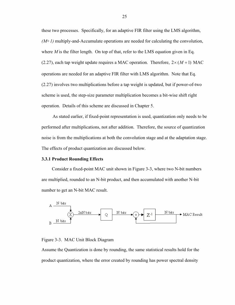
3.3.1 Product Rounding Effects
Consider a fixed-point MAC unit shown in Figure 3-3, where two N-bit numbers
are multiplied, rounded to an N-bit product, and then accumulated with another N-bit
number to get an N-bit MAC result.
Figure 3-3. MAC Unit Block Diagram
Assume the Quantization is done by rounding, the same statistical results hold for the
product quantization, where the error created by rounding has power spectral density

26
of12
2q . Since the adaptive LMS filter contains )1(2 +× M MAC operations, and again
assuming absence of any other noise source, the total error power spectrum produced by
product quantization is
6
)1(12
)1(222 qMqMp
+=+=ε . (3.14)
Given peak power Pc defined in Eq. (3.11), the ratio of the peak power and the product
quantization noise, denoted by Rp is therefore
12
43
6)1(
2 2
2
322
+⋅=
+==
−
MqMqP
Rll
p
cp ε
, (3.15)
or dBMlSNRp 25.1)1log(1002.6 −+−= . (3.16)
For example, a 9th order LMS FIR adaptive filter with 16-bit wordlength has signal to
noise ratio of about 85dB due to product quantization. Again, the calculation is
performed by assuming no any other noise sources.
3.3.2 Coefficient Rounding Effects
In this section, we wish to analyze how product quantization noise is created due to
coefficient rounding in the tap weight adaptation. The LMS algorithm updates the filter’s
coefficients, or tap weights according to Eq. (2.27), which is replicated here:
w(n+1) = w(n) + µu(n)e(n) . (3.17)
As shown in the above equation, the update parameter, namely µu(n)e(n), must be
quantized to less than or equal to wordlength of w(n) in order to produce the proper result
for the updates. Again, the update parameter only involves one set of multiplication if
the step size parameter is power-of-two. The quantization of the update parameter results

27
in quantization noise described in the previous section, that is, for an Mth-order FIR
filter, the tap weight updates result in noise power of12
)1( 2qM + .
Since coefficient quantization is performed on the tap weights, i.e., before the
convolution stage, the quantization noise associated with coefficient quantization is also
process at the convolution stage. Therefore, the adaptive systems are more sensitive
toward coefficient quantization.
Coefficient quantization may result in slowdown or stalling phenomenon, in which
the rate of convergence is either slower or after convergence, tap weights fail to comply
with the weights if infinite precision were used. The slowdown and stalling phenomenon
will be studied in next section. Furthermore, noise produced by coefficient quantization
can be potentially hazardous if an IIR filter structure is used. Since the coefficients
directly affect the stability of an IIR filter, in that any noise introduced in the coefficients
may shift the poles outside of the unit circle and cause the IIR filter to diverge the output.
3.3.3 Slowdown and Stalling
The LMS algorithm may stop adapting due to the finite precision implementation of
the digital hardware. If the result of the update parameter, namely )()( nune ⋅⋅µ is less
than the least significant bit of the binary representation after quantization, that is, if
qnuneQ <⋅⋅ ))()(( µ , (3.18)
where q is the quantizing step, the adaptation fails to update due to the fact that if the
update parameter is less than q, it is quantized into zero.
The step size parameter µ plays an essential role for LMS algorithm stalling. It can
be shown in [7] that by incorporating a lower bound for µ, the stalling phenomenon can
be avoided. The lower bound is described below:

28
224 neu
q
σσσµ
+> , (3.19)
where and denote variance of the error signal and variance of the quantization
noise, respectively. By combining Eq. (3.19) with Eq. (2.28), the range of µ is restricted
to the following:
2eσ 2
nσ
max22
2
4 MSq
neu
<<+
µσσσ
. (3.20)
Also according to [23], with fixed-point arithmetic, it can be advantageous to leave µ as a
higher value when possible.
The sign algorithm is another way of preventing stalling and is presented in [19].
Instead of calculating the update parameter by multiplying the tap and the error term, the
sign algorithm only takes the sign of the error term into consideration. That is, the update
parameter is calculated as following:
[ ])()()()1( nesignnnn uww ⋅⋅+=+ µ . (3.21)
The sign algorithm decreases the chance of stalling and simplifies the hardware
requirements. Since no multipliers are needed to update tap weights, the sign algorithm
also decreases noise created by product quantization. Although the sign algorithm
introduces nonlinearity in the adaptation process, it does not prevent the algorithm from
converging. However, the sign algorithm will always converge slower than the LMS
algorithm [5].
Another method involving dithering is proposed by [16] to prevent stalling. Here
dithers are inserted at the input of the quantizers of update parameters, where a dither
consist of a random sequence that, if added to the input, guarantee the input to be greater

29
than the quantization step. The effect of additive dither can be eliminated by shaping the
power spectrum of the dither so that it is rejected by the algorithm anyways.
The LMS algorithm running under finite precision also may encounter the
slowdown phenomenon, in which the effect of quantization causes the rate of
convergence to be slower than its infinite counter part. In this case, the tap weights may
achieve the intended values only at a slower rate. The slowdown phenomenon can be
eliminated by proper choice of data and coefficient wordlength. It is shown in [15] that
for most practical cases, more bits should be allocated to coefficients than input data to
prevent slowdown.
3.3.4 Saturation
A filter’s internal registers to hold any arithmetic results are fixed. It is possible for
an arithmetic result to overflow during addition and multiplication, that is, the number of
bits to represent the integer part of the summation does not store all the necessary
information. Such a phenomenon is called Saturation. For example, refer to Figure 3-4,
which shows a MAC operation of two N-bit numbers. Saturation may occur when two
N-bit numbers are added to produce an N-bit sum, since (N+1) bits are needed to
represent a full addition without concerning saturation. Similarly, saturation can also
occur when two N-bit numbers are multiplied and the product is quantized to M bits,
where M < 2N. Saturation can introduce major distortions into a system’s output, since
large amount of information is vanished due to the loss of the upper significant bits of the
addition or multiplication result.
Saturation can render a filter useless. Therefore, it is essential for the filter designer
to study the nature of the input data to eliminate the effects of saturation.

30
One of the most common solutions for saturation is to scale the input signals [8].
By scaling down the input signals, the probability of any internal arithmetic overflow is
decreased. However, as suggested in [25], input scaling also decrease the precision of the
data and may result in rough filter outputs or even stalling. This is of particularly
interests for the LMS adaptive filter, since the criteria for the performance of such filter is
the misadjustment of the error signal. Misadjustment, as defined in Chapter 2, is the
difference between the weights produced by the optimum Wiener solution and the
adapted weights produced by the LMS adaptive filter. Therefore, tradeoffs exists as to
the amount of scaling applied to input signal to avoid saturation, at the same time retain
or minimize misadjustment due to the effect of scaling. The only way to achieve such
goal is to carefully study the nature of the input data and calculate the upper bound of the
magnitude of the input signals.
Besides scaling the input signals, increasing wordlength can also reduce the effect
of saturation, that is, to increase the number of bits for each registers. However, this
technique may not be available for some digital implementations. For example, common
DSP processors have fixed wordlength and cannot be modified. Also, wordlength
increment introduces more hardware and reduces the speed of the digital hardware
considerably.
Another way to minimize the effects of saturation is proposed by [25] called
clamping. Clamping will, upon detecting an overflow, clamp the adder’s output to the
most positive or negative values. That is, the output of an N-bit adder is defined as
following:

31
−≤−−<<−
≥−=
−−
−−
−−
11
11
11
2,2122,
2,12
NN
NN
NN
sumsumsum
sumresult (3.22)
Note that Eq. (3.22) assumes 2’s complement form for arithmetic operations.
3.3.5 Solutions for Arithmetic Quantization Effects
Eweda in [10] proposes an algorithm in which the tap weight updates are repeatedly
frozen for a certain period of time and then updating them on the base of the average
innovation period during the freezing period. During each innovation period, the
adaptation parameter, i.e., u(n)e(n) is accumulated and update is only performed at the
end of the innovation period. This innovation period accumulation can smooth out the
quantization errors and therefore increase the output SNR.
It is also shown in [11] that the quantization noise can be reduced exponentially by
increasing the wordlength of the registers. For the same reason stated earlier, this
technique may not be available. If wordlength increment is in fact available, commercial
software exists for wordlength optimization in DSP applications. Such software usually
includes the synthesis tool presented in [18].
3.4 Simulation Result
Throughout this section, one particular application of the LMS algorithm, namely
the system identification application is used. Consider the module depicted in Figure 3-4,
where the LMS adaptive filter is to model the unknown system by using the unknown
system’s output as the desired signal to the adaptive filter. The adaptive filter’s task is to
adapt its tap weights such that its output matches the unknown system’s output.

32
Figure 3-4. System Identification Block Diagram
3.4.1 Rounding vs. Truncation
An experiment is set up to verify the conclusion drawn up from Section 3.1, that is,
for signal quantization, rounding creates less quantization noise than truncation. Refer to
Figure 3-4, both input signal and desired signals are quantized before fed into the
adaptive filter. Arithmetic quantization is not considered at this stage, in other words, the
results from either convolution sum or the adaptation process are not quantized. Since
the LMS algorithm uses minimum mean square error as the criteria, we can safely opt
rounding over truncation if rounding produces less mean square error over truncation.
Figure 3-5. Experimental Setup for Rounding vs. Truncation

33
The two quantization techniques are tested in the two quantizers shown in Figure 3-
5. The adaptive filter length is fixed at four where the input sequence consists of 5000
normally distributed random samples. Additionally, the quantizing step q is chosen to
hold the following values: [2-1, 2-2, 2-3, 2-4, 2-5, 2-6]. At each value of q, the
misadjustment produced by the adaptive system is captured for both rounding and
truncation and the result is shown in Figure 3-6. As shown in Figure 3-6, rounding
clearly produces less noise than truncation for each value of q and only as the
quantization step decreases, the effects of truncation becomes impartial over rounding.
Figure 3-6. Simulation Result for Rounding vs. Truncation
3.4.2 Effects of Product Rounding at the Convolution Stage
In this section, we wish to further experiment the effects from quantization. In
addition to the quantizers shown in Figure 3-7, rounding is also performed at each
multiplication at the convolution stage. Refer to Figure 3-7, for the same 4th-order
adaptive filter used in the previous section, four more quantizers are added.

34
Figure 3-7. Additional Quantizers at the Convolution Stage
We again experiment the effects of product quantization by a set of different q
values [2-1, 2-2, 2-3, 2-4, 2-5, 2-6]. For each value of q, the adaptive filter’s misadjustment
is captured and plotted. The simulation result is shown in Figure 3-7, where as the
quantization step decreases, so does the quantization noise caused by multipliers.
Figure 3-8. Effects of Product Quantization at the Convolution Stage
The figure also verifies the conclusion drawn up in Eq. (3.14), which shows the error
power spectrum decreases exponentially as the quantization step decreases.

35
3.4.3 Effects of Product Rounding at the Adaptation Stage
Coefficient rounding contributes greater quantization noise in the product
quantization noise. In this section, update parameters are also quantized. The same
structure is used as the previous sections and the same set of normally distributed data is
applied. Refer to Figure 3-9, quantization is also performed at the adaptation stage.
Figure 3-9. Additional Quantizers at the Adaptation Stage
Simulation result for this experiment is plotted in Figure 3-10. Note that two sets of
misadjustments were plotted. The red bars correspond to misadjustment due to product
quantization at the convolution stage, whereas the blue bars correspond to misadjustment
due to quantization at the adaptation stage. Clearly, quantization at the adaptation stage
creates significantly larger noise than at the convolution stage for reason stated earlier.
It is apparent that an adaptive filter’s performance is more sensitive to coefficient
quantization noise. Thus, as suggested in Section 3.3.3, more bits should be allocated for
coefficient representation.

36
Figure 3-10. Effects of Product Quantization at the Convolution and Adaptation Stages
3.4.4 Clamping Technique
An experiment is setup to simulate the saturation phenomenon on an adaptive LMS
filter. System identification practice described in Figure 3-4 again is used, where tap
weight adaptation is performed so that the adaptive filter’s output matches the unknown
system’s output. For simplicity, all inputs are positive. An upper bound is set for
wordlength of results from either multiplications or additions. If wordlength of the result
exceeds this upper bound, two scenarios are tested, one is to do nothing, that is, the upper
most significant bits are lost due to saturation; the other is by the use of clamping, in
which upon detection of saturation, the result is clamped to most positive number that the
upper bound can represent. A set of normally distributed data is tested in this
experiment, where the adaptive filter’s ideal tap weights are [4 5 1] after convergence.
The results of this experiment are shown in Figure 3-11 and Figure 3-12, where both the
misadjustment curve and the tap weights are plotted.

37
Figure 3-11. Tap weight Track for Clamping Technique
In Figure 3-11, the blue lines track tap weights if no clamping were used whereas
the red lines track tap weights if clamping were used. The black lines represent the ideal
tap weights if a 64-bit floating-point system were used, which is considered ideal. It is
apparent that tap weights simply diverge if clamping is not used. The divergence of the
tap weights indicates the adaptive filter has become ineffective.
Figure 3-12 shows the misadjustment plot of the experiment. The mean square
error of each system is capture at every 30 samples. As can be seen, the mean square
error of the non-clamping result is never reduced due to tap weight divergence whereas in
the clamping case, the misadjustment is very close to the ideal result.

38
Figure 3-12. Misadjustment Plot for Clamping Technique
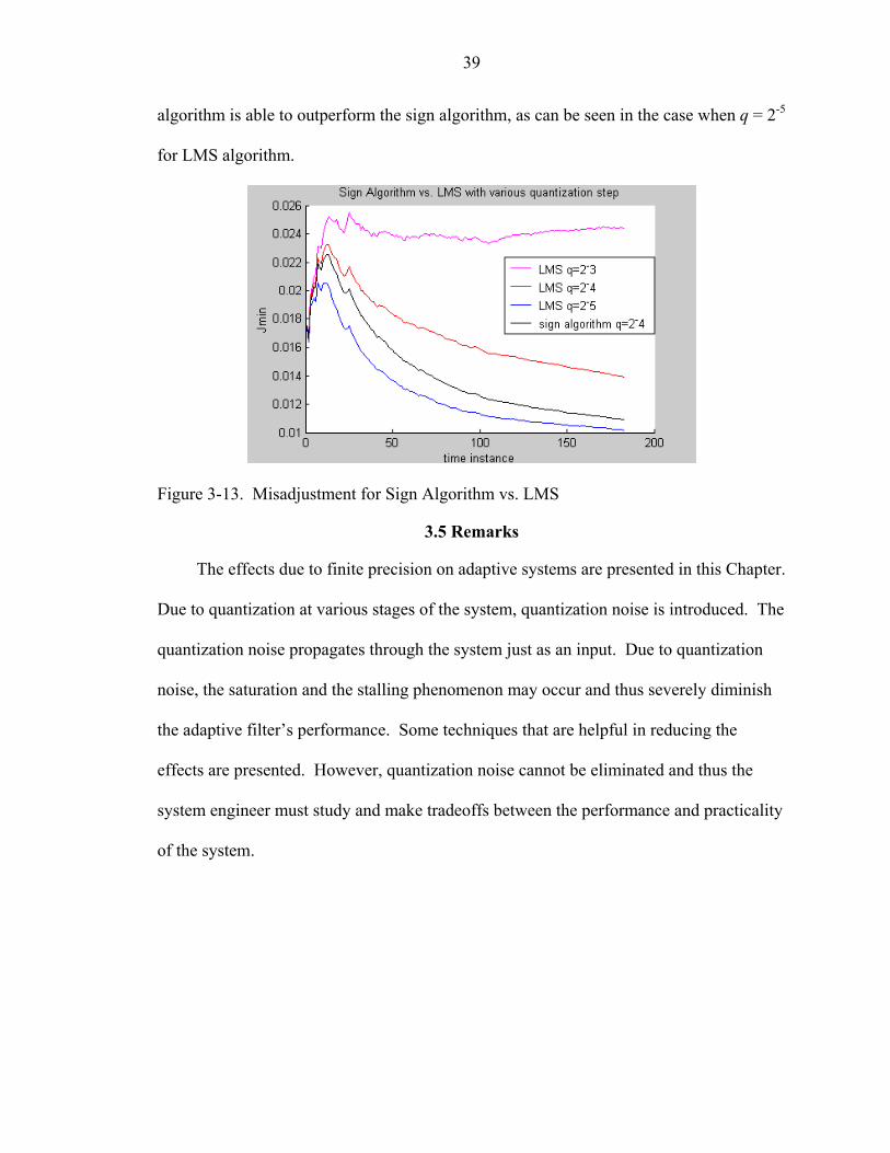
3.4.5 Sign Algorithm
The sign algorithm presented in the previous section is a way of preventing stalling
when the update parameter result is less than the quantizing step. System identification is
again used in this simulation. A set of small scale input and desired signal are used and
various quantizing step values are tried. It was determined that for q < 2-4, tap weights
simply diverge. Therefore, quantizing steps q = [2-3, 2-4, 2-5] are used for this experiment.
The effectiveness of the sign algorithm with respect to the LMS algorithm using various
q values is studied. Figure 3-13 shows the misadjustment plot for the adaptive filter with
same sets of input and same filter order with respect to various q values. Misadjustment
is again captured at every 30 samples. The step size for the sign algorithm is slightly
larger than the LMS algorithm in order for it to converge due to reason stated in [7]. As
shown in Figure 3-13, tap weights diverge when q = 2-3 due to insufficient fractional bits.
In the case of q = 2-4, due to limited precision, the LMS algorithm stalls and results in
larger misadjustment than the sign algorithm, that is, the sign algorithm is able to obtain
better convergence result than the LMS algorithm. Only by decreasing q, the LMS
39
algorithm is able to outperform the sign algorithm, as can be seen in the case when q = 2-5
for LMS algorithm.
Figure 3-13. Misadjustment for Sign Algorithm vs. LMS
3.5 Remarks
The effects due to finite precision on adaptive systems are presented in this Chapter.
Due to quantization at various stages of the system, quantization noise is introduced. The
quantization noise propagates through the system just as an input. Due to quantization
noise, the saturation and the stalling phenomenon may occur and thus severely diminish
the adaptive filter’s performance. Some techniques that are helpful in reducing the
effects are presented. However, quantization noise cannot be eliminated and thus the
system engineer must study and make tradeoffs between the performance and practicality
of the system.

CHAPTER 4 SOFTWARE SIMULATION OF A FIXED-POINT-BASED POWER-OF-TWO
ADAPTIVE NOISE CANCELLER
The effects of finite precision are elaborated in Chapter 3. In this Chapter, we wish
to translate theories into reality, where a floating-point based system is compared with a
fixed-point based system. As stated in Chapter 3, a floating-point based system can
represent larger dynamic range of data in the cost of losing resolution and introducing
more quantization noise, where a fixed-point-based system’s dynamic range is limited
with respect to its quantizing step, but holds the advantage of simpler circuit design, since
additions and multiplications are composed of simpler logic equations. Therefore, for
implementation of a finite precision adaptive system, fixed-point architecture is preferred
over floating-point. It is the goal of this chapter to obtain the feasibility of implementing
fixed-point based adaptive system due to its simplicity.
As described in Chapter 2, the LMS algorithm is the most widely used adaptive
algorithms and bears many applications. Two examples were explored in Chapter 2,
namely the noise canceller and the line enhancer. In this Chapter, a software simulation
of a noise canceller is implemented and the LMS algorithm is fixed-point based. The
step size parameter utilizes power-of-two scheme, that is, µ can only take up values
of , where n is a positive integer. n−2
Consider a scenario where a speaker is giving out a speech, while the housekeeper
insists on vacuuming the floor at the same time. The vacuuming noise obscured the
speech to an extend that it was not audible. The contaminated speech, i.e., original
40
41
speech plus noise, and the noise itself are recorded. An experiment is set up to use the
Adaptive Noise Canceling technique to retrieve the original speech. The noise signal
itself serves as the primary filter input, and the contaminated signal is the reference input,
or the desired signal to the system. We wish to investigate the effect of finite wordlength
due to this particular application. Specifically, can the speech be recovered by this
integer-based system? And how much does this fixed-point-based system differ from a
floating-point based counterpart? If the fixed-point-based system makes no striking
difference on the outcome of noise canceller, i.e., the original speech can still be
recovered and be heard by human, then a hardware implementation based on this
software experiment becomes feasible since fixed-point-based adaptive system is ideal
due to its simplicity and practicality.
4.1 Modular Overview
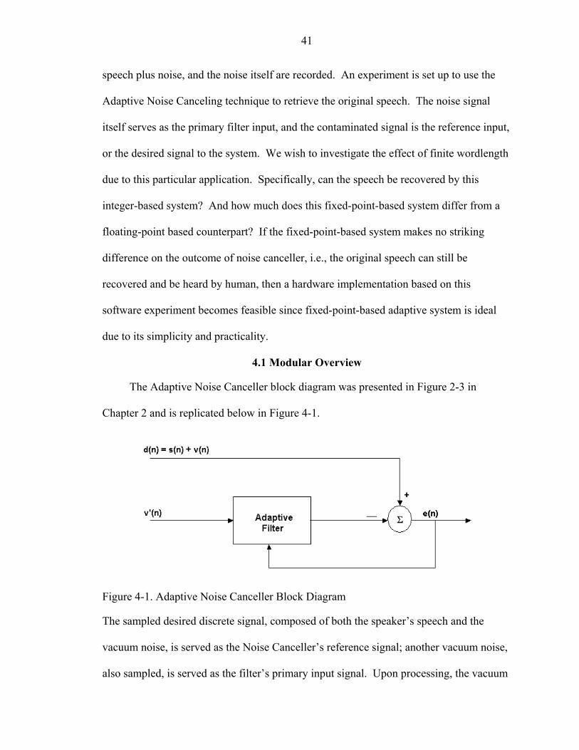
The Adaptive Noise Canceller block diagram was presented in Figure 2-3 in
Chapter 2 and is replicated below in Figure 4-1.
Figure 4-1. Adaptive Noise Canceller Block Diagram
The sampled desired discrete signal, composed of both the speaker’s speech and the
vacuum noise, is served as the Noise Canceller’s reference signal; another vacuum noise,
also sampled, is served as the filter’s primary input signal. Upon processing, the vacuum

42
noise will be reduced due to the adaptation of the filter tap weights. And the error signal
produced by the adaptive system is in close resemblance of the original speech.
Figure 3-4 shows the internal structure of the adaptive filter, including the
quantizers to quantize all inputs and tap weights to fixed wordlengths. The filter uses tap
delay line architecture and thus, for an Mth-order filter, M+1 multiplications are needed
at the convolution stage and M+1 more at the adaptation stage.
Figure 4-2. Internal Structure of the Noise Canceller with Quantizers
4.2 Data Quantization
As seen in Figure 4-2, quantization takes place in four stages: at the primary input
signal, the reference signal, and in both convolution and adaptation. Rounding is used for
quantization. Since the primary and reference signal quantization is unavoidable due to
A/D conversion, the only source of error that can be controlled by the designer is then
product quantization noise at both the convolution stage and the adaptation stage. The
quantizing step determines how many fractional bits are remained after quantization. It is
established that product quantization noise is inversely exponential with respect to
quantizing step.

43
4.3 Simulation Results
The primary and reference signals are assumed proper sampled. By
experimentation, the filter length is chosen to be four and the step size µ is chosen to
be . A set of quantizing steps, q = [2-5, 2-6, 2-7, 2-8], are used to show the
misadjustment due to product quantization error. For simplicity reason, the number of
bits to represent integer parts of products is assumed to be sufficient, that is, saturation is
not considered in this experiment. Figure 4-3 and 4-4 show the weight tracks and the
misadjustment curves with respect to various values of q, respectively. The performances
of the four fixed-point systems are compared against a 64-bit floating point system. As
can be seen in the figure, when q = 2-8, the fixed-point system performs just as well as the
floating-point system. More importantly, although the speech filtered by the fixed-point-
based system is noisier, largely due to quantization noise, the recovered speech tends to
be intact and coherent.
72−
Figure 4-3. Weight Tracks for Fixed-point Systems

44
Figure 4-4. Misadjustment Plots of Fixed-point Systems and a Floating-point System
The success of this software experiment proves that for adaptive applications such
as noise cancellations, the system is not as sensitive to input A/D conversion and data
quantization. And as can be shown in simulation, fixed-point systems with limited
quantizing step perform just as well as a 64-bit floating-point system. Without sacrificing
enormous amount of hardware if a floating-point system were applied, hardware
implementation of a fixed-point system therefore becomes very appealing and feasible.
In fact, Chapter 5 illustrates a VLSI based noise canceller that is fixed-point-based and
takes advantages of the power-of-two scheme.

CHAPTER 5 HARDWARE IMPLEMENTATION OF AN INTEGER-BASED POWER OF TWO
ADAPTIVE NOISE CANCELLER IN STRATIX DEVICES
Chapter 4 presented a software simulation of an adaptive noise canceller based on
fix-point approach. By experimenting the fixed-point based system, it is believed that
noise cancellers are one of the adaptive applications that are practical for a fixed-point-
based hardware implementation.
DSP applications, including adaptive algorithms involve heavily upon arithmetic
operations such as multiplication and addition. By incorporating fixed-point only, adder
and multipliers that are essential to DSP applications require less amount of logic
elements as opposed to if the applications were implemented in floating-point based. In a
VLSI circuit design, this feature is particular of interest, since VLSI devices have limited
logic elements and simpler circuit generally translates into faster performance.
The newest FPGA families, Altera’s Stratix device family for example,
incorporates embedded DSP blocks within the FPGA chip to have dedicated circuitry to
perform common DSP operations including multiply and accumulate. This family of
FPGA devices is compared with another family of FPGA devices that does not include
embedded DSP blocks. Performance comparison is done in two areas, which include
amount of logic elements occupied and maximum frequency allowed. The power-of-two
scheme is used to avoid implementing area-consuming division circuitry.
45
46
Software package Quartus II is used to produce a waveform simulation, along with
logic state analyzer's captured waveform are presented to verify the hardware
functionality.
DSP applications including adaptive systems have traditionally been implemented
using general-purpose DSP processors due to their ability to perform fast arithmetic
operations. Advancement in FPGA devices including the embedded DSP blocks has
made FPGA devices serious contenders in the DSP market. It is advantageous to
examine the performance of the adaptive filter implemented in Stratix devices against
both fixed-point based DSP processor and floating-point based DSP processor. Two
criteria, system speed and power consumption are examined and the results are shown in
this Chapter.
5.1 Stratix Devices
5.1.1 Device Architecture
The Stratix family is the newest family of programmable logic devices from Altera.
The Stratix devices have three times the size of memory blocks compared to traditional
FPGAs. The Stratix devices also contain embedded DSP blocks, which have dedicated
pipelined multiplier and accumulator circuits. With the embedded DSP blocks, the
Stratix devices can perform high speed multiply-and-accumulate operations.
Stratix devices contain a two-dimensional row and column based architecture to
implement custom logic. A network of varying length and speed, row and column
interconnects provide signal interconnections between Logic Array Blocks (LABs),
memory blocks, and embedded DSP blocks. Each LAB consists of 10 Logic Elements
(LEs). LABs are grouped into rows and columns across the device. The memory blocks
are RAM based. These memory blocks provide dedicated simple dual-port or single port

47
memory up to 36 bits wide and up to 291MHz access speed. The DSP blocks can
implement multiplications in various bit length with add or subtract features. The blocks
also contain 18-bit input shift registers for applications such as Finite Impulse Response
(FIR) or Infinite Impulse Response (IIR) filters. Figure 5-1 shows the block diagram of a
typical Stratix device [2].
Figure 5-1. Stratix Device Block Diagram
5.1.2 Embedded DSP Blocks
The most commonly used DSP functions include multiplication, addition, and
accumulation. The Stratix devices provide DSP blocks to meet the arithmetic
requirements of these functions. Each Stratix device has two columns of DSP blocks to
efficiently implement DSP functions faster than LE-based implementations.
Each DSP block can be configured to support one set of the following:
• Eight 9 x 9 bit multipliers
• Four 18 x 18 bit multipliers
• One 36 x 36 bit multiplier

48
DSP block multipliers can optionally feed an adder/subtractor or accumulator within
the block. This feature saves LE routing resources and increase performance, since all
inter-connections and blocks are all within the DSP block. The DSP block input registers
can also be configured as shift registers for FIR filter applications. Figure 2 is a block
diagram for a typical component inside the DSP block.
Figure 5-2. Embedded DSP Block Diagram
5.2 Design Specifications
5.2.1 Structural Overview
The noise canceller implementation assumes FIR filter structure. The design shown
in Figure 5-3 depicts a structural view of such FIR filter. As shown in the figure, the
main components of the filter consist of m Unit Delay Registers and m+1 Weight
Updates. The Unit Delay Registers are simply D Flip-Flops. Each Weight Update
component updates the filter coefficient according to the LMS equation presented in
Chapter 2, Eq. (2.27). The adaptive filter’s input is the primary input, which is the
vacuum noise. The filter output is subtracted from the desired signal, in this case, the

49
original speech plus noise, to produce an error signal. The error signal, i.e., the recovered
speech is a buffer, which is fed back to the Weight Update components to produce next
sets of filter coefficients.
Figure 5-3. Adaptive Transversal Filter Block Diagram
5.2.2 The Power-of-Two Scheme
Weight Updates perform logics according to Eq (2.27). Arithmetic operations
needed include two multiplications and one subtraction. However, the step-size
parameter µ is a fractional number that is always less than 1. Also, by multiplying a
fractional number is equivalent of dividing its reciprocal. Therefore, in order to avoid
implementing complicated and area-consuming division circuitry, or multiplication for
floating-point numbers, Arithmetic Shift Right (ASR) operation is used instead to
simplify and boost the run-time frequency of the design.
The ASR operates on a 2’s complement integer by shifting the number n bits to the
right (direction of the least significant bit), while preserving the sign bit (the most
significant bit). By shifting the number n bits to the right, it is equivalent of multiplying
this number by 2-n. Therefore, in order to achieve simplicity and feasibility, this design
restricts the value of µ to be µ = 2-n, where n is a positive integer. This is the so-called
power-of-two scheme.
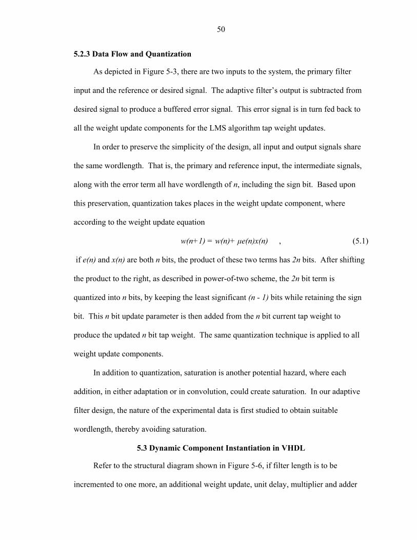
50
5.2.3 Data Flow and Quantization
As depicted in Figure 5-3, there are two inputs to the system, the primary filter
input and the reference or desired signal. The adaptive filter’s output is subtracted from
desired signal to produce a buffered error signal. This error signal is in turn fed back to
all the weight update components for the LMS algorithm tap weight updates.
In order to preserve the simplicity of the design, all input and output signals share
the same wordlength. That is, the primary and reference input, the intermediate signals,
along with the error term all have wordlength of n, including the sign bit. Based upon
this preservation, quantization takes places in the weight update component, where
according to the weight update equation
w(n+1) = w(n)+ µe(n)x(n) , (5.1)
if e(n) and x(n) are both n bits, the product of these two terms has 2n bits. After shifting
the product to the right, as described in power-of-two scheme, the 2n bit term is
quantized into n bits, by keeping the least significant (n - 1) bits while retaining the sign
bit. This n bit update parameter is then added from the n bit current tap weight to
produce the updated n bit tap weight. The same quantization technique is applied to all
weight update components.
In addition to quantization, saturation is another potential hazard, where each
addition, in either adaptation or in convolution, could create saturation. In our adaptive
filter design, the nature of the experimental data is first studied to obtain suitable
wordlength, thereby avoiding saturation.
5.3 Dynamic Component Instantiation in VHDL
Refer to the structural diagram shown in Figure 5-6, if filter length is to be
incremented to one more, an additional weight update, unit delay, multiplier and adder

51
are all needed to be instantiated. But both the length of the adaptive filter and the
wordlength to represent data bus should be easily changed without spending too much
time on the architectural level. Since this adaptive filter is written in VHDL, we now
show how to dynamically instantiate a component in VHDL.
In a separate “header” file, a package is created to include not only the components
definition, but also constants such as filter length and bus width information. A portion of
the “header” file is shown below:
This header file is included into the project and upon compiling, the package information
is used in the structural port map statements in the top hierarchy to determine the number
of components to be instantiated. Therefore, by changing the numbers in the package
field, the designer is able to dynamically instantiate however many number of
components needed for the specific design. For additional helpful VHDL tutorials please
refer to [26].

52
5.4 Simulation and Implementation Results
It can be argued that since input signals have to be converted from analog to digital,
and A/D operations involves converting real values into 2’s-complement binary values,
adaptive systems are therefore naturally suitable for integer-based. The sampled primary
and reference signals are scaled and rounded to be integers before it is fed into the
system.
Altera’s Quartus II software package is used to compile the VHDL-based package
and a vector waveform simulation is produced. The primary and reference signals are
stored into the device’s internal memory with equal depth. Update parameter remains the
same throughout the process, while the address line that controls the internal memory is
incremented in every clock cycle. A snapshot of the waveform simulation is captured
and shown in Figure 5-4. Upon convergence, the tap weights become [0001, FFFA,
FFFF, 0002, FFFD]. Converting these hexadecimal numbers into decimal, the weights
are [1, -6, -1, 2, -3].
Figure 5-4. Waveform Simulation Result of the Adaptive Noise Canceller

53
The project is implemented into Altera's DSP development board and the lower 5
bits of each weight are captured using a logic state analyzer. The analyzer's result is
shown in Figure 5-5 below.
Figure 5-5. Logic State Analyzer Result of the Adaptive Noise Canceller
Implementation result shows that lower 5-bits of the weights are [00001, 11010, 11111,
00010, 11101]. 2’s complement forms are indeed [1, -6, -1, 2, -3], which are equivalent
to the waveform simulation demonstrated in Figure 5-4.
5.5 Performance Comparison of Stratix and Traditional FPGAs
Area and speed are the two main measurements in evaluating FPGA performance of
this filter. Since the Stratix devices have embedded DSP blocks built in, they should
occupy less LEs and have faster maximum clock frequency. Area and Speed issues were
studied with a Stratix Device and a FPGA device without embedded DSP blocks, namely
an APEX device also from Altera. Figures 5-5 and 5-6 show the varying filter orders vs.
area and speed plots, respectively, for both the Stratix and APEX devices. Area is
measured by number of LEs occupied, whereas speed is measured by longest register-to-
register delay.

54
5.5.1 Speed
Refer to Figure 5-3, for each additional tap, the longest register-to-register path is
elongated as well, resulting allowable frequency to plunge. Figure 5-6 shows as the
number of taps increase, the allowable speed of the adaptive filter decreases, that is, the
clock frequency decreases. Timing for Stratix device is obtained from Quartus
simulation result, since a Stratix device is not readily available. For the APEX device,
timing is obtained by using a functional generator to generate a clock signal as the
system's clock signal. Clearly, if the functional generator's clock signal period exceeds
the longest register-to-register delay, it will cause erroneous computational result, since
logic elements need the time period specified by longest register-to-register delay to
perform correct computation. Therefore, the maximum frequency is obtained from the
fastest frequency in which the adaptive system can run while still able to obtain intended
tap weight convergence.
05
10152025303540
Max.Freq. (MHz)
3 5 10 25 35 50Filter Order
StratixAPEX
Figure 5-6. Plot of Filter Order vs. Speed
5.5.2 Area
For each additional tap, a separate weight update, multiplier, and adder also have to
be instantiated. These components all occupy LEs. Therefore, when the number of taps

55
increases, so does the number of occupied LEs. Figure 5-7 shows this relationship. Note
that for the Stratix device at filter length of 20, all embedded DSP blocks have been
occupied with multipliers and adders. The DSP block elements do not count as logic
elements. Each additional multiplier and adder required by the increase of filter length,
they is implemented in regular LEs, which results in a exponential growth from filter
length 10 to filter length 25.
0100002000030000400005000060000
LEs
3 5 10 25 35 50Filter Order
Stratix
APEX
Figure 5-7. Plot of Filter Order vs. Area
From the above two graphs, we can easily see that the Stratix device is
overwhelmingly favored over traditional FPGA devices. When it comes to DSP
applications implemented in FPGA devices, the Stratix device not only occupies less LEs
due to the dedicated circuitry within the DSP blocks, but it also allows faster clock
frequency.
5.6 Pipelining
Although the design depicted in Figure 5-3 fully utilizes the parallelism advantage
of FPGA devices in full, the speed performance decays substantially as the filter order
increases, since the longest register-to-register delay elongates from the first weight

56
update component on the left to the subtractor on the right. Two methods can be
incorporated into the existing design to reduce the longest register-to-register delay. The
first method is to introduce pipelined multipliers. Multipliers occupy large amount of
logic, by partitioning the entire multiplier logic into smaller elements and incorporate
pipeline registers in between, the register-to-register delay can be decreased, resulting in
an increase of the maximum system clock frequency. The other method involves
inserting buffers into the chain of adders at the convolution stage. The amount of
sequential adders increases linearly as filter order increases. Therefore the amount of
LEs to implement these adders also increases, resulting in an overwhelming decrease in
system speed. If buffers are added into the adder-chain, the system's maximum data rate
can be increased. The two methods can be combined together to obtain an adaptive
system with optimal performance in terms of data rate.
Latencies are also introduced by incorporating the above two methods. Latencies
introduced in multipliers or in adder-chain effectively create phase shifts into the
convolution stage, since full result of the multiplication is delayed by the number of
pipeline levels. Consequently, this phase shift also affects the error output signal because
error output is also delayed. If the phase shift created by latency becomes sufficiently
large, it can remove the correlation between the reference signal and the primary signal
and force the adaptive system to diverge. In fact, the error produced by the adaptive
system is a function of the primary and reference signals, and the error signal is also a
feedback signal to the weight updates. We will, in this section, investigate techniques to
cope with latency effects in adaptation.

57
Synthesis tools that partition the multiplier logic can be investigated to obtain
optimal number of pipeline stages. Optimal number of pipeline stages is defined as the
smallest number of pipeline stages for which further increase does not enhance
multiplier’s speed. The maximum speed of the pipelined multiplier serves as a guideline
to how many buffers are inserted into the adder-chain. We wish to insert minimal
number of buffers onto the adder-chain to minimize latencies, and also to minimize
register-to-register path. Procedures on how to obtain optimal pipeline stages are now
discussed.
5.6.1 Optimal Multiplier Pipeline Stages
In order to investigate the synthesis tool provided by Quartus software, a multiplier
block is instantiated according to Figure 5-8. Without pipelining the multiplier, the
longest register-to-register delay is from the input register to the output register. If
pipelines are introduced within the multiplier, the longest register-to-register delay is
reduced.
Figure 5-8. Pipelined Multiplier Test Module
Performance improvement in speed with various numbers of pipelines for different
sizes of multipliers is studied using the Quartus synthesis tool. It can be shown according
to Figure 5-9 that, for an 8-bit multiplier, the optimal pipeline stage is 1, since
incrementing the number of pipeline stages does not generate better multiplier

58
performance. Similarly, the optimal pipeline stages for 16-bit multiplier and 32-bit
multiplier are 2 and 3, respectively.
0
50
100
150
200
250
300
350
400
0 1 2 3 4
Pipeline Stages
Mul
tiplie
r Dat
a R
ate
(MH
z)
8-bit16-bit32-bit
Figure 5-9. Maximum Data Rate of three Multipliers with Various Pipeline Stages
5.6.2. Optimal Adder-chain Pipeline Stages
Refer to the structural diagram in Figure 5-3, adders used in convolution may
become a burden to system performance in terms of speed, because the adder-chain
occupies more logic elements as filter order increases. As discussed in the previous
section, multipliers can be pipelined in optimal pipeline stages with respect to their input
bus size. In this section, we wish to investigate further improvement in the adaptive
system's speed performance by inserting buffers into the adder-chain. The goal is to
minimize the number of buffers while not increasing the longest register-to-register
delay. It is apparent that the upper bound constraint for the number of adders in between
buffers should be less than the speed of the pipelined multiplier.
According to results found in the previous section, an 8-bit, 16-bit, and 32-bit
multiplier can be pipelined and have optimal speed of 335MHz, 278MHz, 278MHz,

59
respectively. An adder-chain component described in Figure 5-10 is instantiated to
observe the number of adders that can be included within the multiplier's speed range.
Figure 5-10. Adder-chain Test Module
Results of 8-bit, 16-bit, and 32-bit adders are shown in Figure 5-11. For 8-bit
adders, it is found that in order to satisfy the speed constraint set by the multipliers, one
buffer can be added for every two adders in the adder-chain to optimize system
performance. Three adders between buffers already exceed the propagation delay of an
8-bit pipelined multiplier. Similarly for 16-bit and 32-bit adders, the maximum numbers
of adders that can be included between two buffers are also two.
0
50
100
150
200
250
300
350
400
450
1 2 3
Number of Adders in Adder-Chain
Add
er D
ata
Rat
e (M
Hz)
8 bit
16 bit
32 bit
Figure 5-11. Adder-chain Data Rate with Respect to Number of Adders
Incorporating pipelined multipliers and buffering adders in the adder-chain can
reduce the longest register-to-register delay. As an example, the structural view of a 4th-

60
order adaptive system is shown in Figure 5-12 below, where multipliers are pipelined
with two stages and buffers are added for every two adders in the adder-chain.
Figure 5-12. Pipelined and Buffered Adaptive System Block Diagram
Note that since a buffer is added after the second adder on the adder-chain, buffers
are also added to the fourth and fifth multiplier outputs in order to compensate the latency
introduced by the adder-chain buffer.
5.6.3 Tradeoffs in Introducing Latency into Adaptive Systems
As described earlier, an adaptive system consists of both convolution and
adaptation stages. These two stages are expressed mathematically in Eq. (2.25) – Eq.
(2.27). By introducing pipelining and buffers, an adaptive system can be expressed in the
following two equations representing error signal computation and adaptation:
)()()()( nDnTndne uwD −−= , (5.2)
)()()()1( nnenn uww Dµ+=+ , (5.3)
where D represents levels of latencies and eD represents delayed error signal. As
described earlier, if latency is large, an adaptive system can due to phase shift caused by
latencies.

61
Recall that the criteria for the step size parameter µ is derived in Chapter 2, in that
µ must satisfy the following inequality:
max
10λ
µ << , (5.4)
where maxλ is the largest eigenvalue of R. It can be shown in [17] that in order to
guarantee convergence of the adaptive system with latencies, µ must be restricted to an
even smaller constraint:
)12(2sin20
max +<<
Dπ
λµ . (5.5)
Note that Eq. (5.5) also shows that as number of pipeline stages increase, range for
appropriate µ decreases.
It can also be shown in [17] that a pipelined LMS system always converges slower
than an un-pipelined LMS system. Several authors have investigated in improving the
pipelined LMS systems' convergence rate. In [9], a correction term is incorporated into
generating the error signal in that
)()()()()( ncnDnTndne uwD −−−= , (5.6)
)1()()( )( −= nEnRnc DT , (5.7)
where RT(n) is the D-dimensional input correlation vector and E(D)(n-1) is a vector of past
errors. It was shown that the modified method of calculating error signal results in equal
performance with respect to un-pipelined LMS system. However, more computation is
introduced as well and thus essentially nullifies the purpose of pipelining. Convergence
rate can also be improved by updating the weight according to LMS algorithm, at the

62
same time modifying the step size according to the following update equation proposed
in [28]:
)()()()(
)()1( DneDnDnDn
nn uuuww T −−−−
+=+µ . (5.8)
Again this method introduces more computation overhead and thus is not desired. In
addition, the software tool MMAlpha is used in [13] to automatically derive a VHDL
description of a pipelined LMS architecture to optimize speed and sacrificing 50%
increase in area.
Based upon evidence presented above, by introducing pipelines into the adaptive
system, the system’s speed is increase in the expense of either slower convergence rate or
more computation. However, by aligning the terms shown in Eq. (5.2) and (5.3), we can
reduce the effects of phase shifts caused by pipelining. Refer to structural diagram
depicted in Figure 5-12. If multipliers are pipelined, and buffers are added to adder-
chain, latencies are propagated into the error signal calculation. The delayed error signal
is fed back into the weight update components to perform adaptation. Buffers can be
added onto the system's reference signal to align the error signal calculation.
Furthermore, weight updates can also be aligned by using delayed filter taps. This time
alignment scheme can be expressed by the following three equations:
)()()( nnTny uwD = , (5.9)
)()()( nyDndne DD −−= , (5.10)
)()()()1( Dnnenn uww D −+=+ µ . (5.11)
With this scheme the weight update at sample n is done with the input and desired signals
at sample n-D. For signals that do not change a lot between sampling points, this scheme

63
provides a close fit to the un-pipelined architecture. This means over-sampling is
suggested when using the time-align scheme. Otherwise there will be a penalty in
convergence rate. The new architecture applied to the structure depicted in Figure 5-12 is
shown in Figure 5-13 below:
Figure 5-13. Time-aligned Adaptive System Block Diagram
Compared with previous solutions described in literature mentioned earlier, this time
alignment scheme does not introduce more computation. It does, however, introduce
more hardware in terms of buffers. The convergence rate for this pipelined system is still
slower than an un-pipelined system.
5.6.4 Performance of the Pipelined Adaptive System
Performance of the un-pipelined design in terms of speed is illustrated in Figure 5-
5. In this section, pipelines are added into the multipliers as shown in Figure 5-3. The
pipelined adaptive system is compared against the un-pipelined system. Buffers are
further added into the adder-chain. The Stratix device is used for the implementation.
The multiplier bus width is set at 16 and thus according to Figure 5-9, optimal pipeline
stage is set at 2. Buffers are inserted for every two adders within the adder-chain. By
varying the filter order in the system, maximum data rates of three scenarios are plotted

64
in Figure 5-14 with respect to filter orders. The three scenarios are the following: an un-
pipelined system, a pipelined system, and a system with pipelined multipliers and buffers.
0
10
20
30
40
50
60
70
Max
Fre
q (M
Hz)
3 5 10 25 35 50
Filter Order
un-pipelined
pipelined
pipelined and buffered
Figure 5-14. Pipelined Adaptive System Performance
Note that although a pipelined-and-buffered adaptive system can have maximum data
rate up to 60MHz regardless of filter order, it also has the most stages of latency.
To summarize, an adaptive system's speed performance can be increased
significantly by either pipelining multipliers, adding buffers onto the adder-chain, or
both. Latency is introduced such that the adaptive system may diverge its tap weight
adaptation, due to the delayed error signal is also a feedback signal to weight updates.
Buffering the desired signal can time-align the error signal computation and the tap
weight update computation. The time-aligned scheme does not require correction terms
described in Eq. (5.6), nor does it require modifying the step size as described in Eq.
(5.7). Experiments have shown that the time-align scheme reduces the effects of latency.
However, since latency cannot be completely compensated, convergence rate for the
time-aligned adaptive system is still slower than an un-pipelined adaptive system. In

65
real-time applications where high data rates are given, slower convergence rate can be an
acceptable tradeoff [20].
5.7 Performance Comparison of FPGAs and DSP Processors
DSP applications have traditionally been implemented with DSP processors. Due
to recent advancement in FPGA devices, it is valuable to compare the performance of
adaptive system in both FPGA devices and DSP processors in terms of speed and power
consumption.
FPGAs maintain the advantages of custom functionality while avoiding the high
development costs and the inability to make design modifications after production [14].
Compare with DSP processors, FPGAs also hold the advantage of parallelism, in that
multiple operations can be performance at one time instance, whereas DSP processors are
only able to perform one instruction per time instance. It is evident that according to
Figure 5-3, by instantiating multiple adders and multipliers, the system is able to perform
convolution and adaptation on the fly. If the design is implemented in DSP processors,
then only one instruction is performed at a time. However, it is also apparent that as the
filter order increases, so does the register-to-register delay in FPGA design, which will
eventually overcome the parallelism advantage. Therefore, performance in terms of
speed is investigated using two devices, namely the Stratix FPGA device and Texas
Instruments' TMS320VC33 floating-point DSP processor.
Power consumption is also a main concern in choosing between various devices.
Power consumption is assumed fixed for DSP processors, since the internal structure is
fixed. FPGA devices’ power consumption varies with respect to amount of LEs
programmed, number clock-driven registers, and DSP block utilization. Issue of power

66
consumption is also investigated in this section using Stratix device, a floating-point
processor and a fixed-point processor.
5.7.1 Speed
Pipelined adaptive system presented in Section 5.5 is used to compare with a
floating-point DSP processor. The processor of choice is Texas Instruments’
TMS320VC33 floating-point DSP processor. The floating-point processor has maximum
speed of 150 Million Floating-Point Operations per Second (MFLOPS) at 60MHz.
Speed is measured by amount of time it takes to update a set of weights for an adaptive
system with various number of filter order. Based on benchmark data obtained from Mr.
Scott Morrison of Computational NeuroEngineering Laboratory, University of Florida,
for a single channel LMS adaptive filter, the C33 processor updates tap weights in the
order of microseconds where as the FPGA LMS adaptive filter can perform tap weight
updates in the order of nanoseconds. For example, it takes the APEX device
implementation 67ns to update all tap weights for an adaptive filter of order 10, whereas
it takes the DSP processor 2.3µs to do so. Parallelism works in full advantages over DSP
processors in this LMS adaptive application. A shortcoming for FGPA implementation
however, is that the amount of LEs are limited for a given device, which restricts the
order of filter to be fit in a particular FPGA. There is no such problem for DSP
processors, since they rely on either internal or external memory to store information, and
computations are done sequentially. Furthermore, floating-point implementation is not
yet feasible in FPGA devices, because the devices have limited LEs. For any
applications that require large data dynamic range, DSP processors still are devices of
choice.
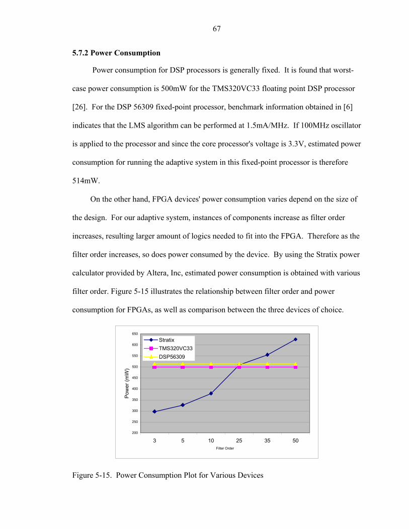
67
5.7.2 Power Consumption
Power consumption for DSP processors is generally fixed. It is found that worst-
case power consumption is 500mW for the TMS320VC33 floating point DSP processor
[26]. For the DSP 56309 fixed-point processor, benchmark information obtained in [6]
indicates that the LMS algorithm can be performed at 1.5mA/MHz. If 100MHz oscillator
is applied to the processor and since the core processor's voltage is 3.3V, estimated power
consumption for running the adaptive system in this fixed-point processor is therefore
514mW.
On the other hand, FPGA devices' power consumption varies depend on the size of
the design. For our adaptive system, instances of components increase as filter order
increases, resulting larger amount of logics needed to fit into the FPGA. Therefore as the
filter order increases, so does power consumed by the device. By using the Stratix power
calculator provided by Altera, Inc, estimated power consumption is obtained with various
filter order. Figure 5-15 illustrates the relationship between filter order and power
consumption for FPGAs, as well as comparison between the three devices of choice.
200
250
300
350
400
450
500
550
600
650
3 5 10 25 35 50Filter Order
Pow
er (m
W)
StratixTMS320VC33DSP56309
Figure 5-15. Power Consumption Plot for Various Devices

68
As seen in Figure 5-15, if energy conservation is desired, FPGA implementation
should be considered over the two DSP processors for an adaptive filter with filter order
less than 25. For filter order over 25, Stratix device consume more energy than the DSP
processors and therefore becomes unattractive.

CHAPTER 6 CONCLUSION AND FUTURE WORK
6.1 Conclusion
Finite precision effects on adaptive algorithms have been studied in this thesis.
Several common effects were studied and solutions were provided to mitigate the effects.
An adaptive noise canceller was first simulated in software for its effectiveness in an
integer-based system. The noise canceller was then implemented in a VLSI-based
hardware due to its success in software simulation.
One commonly used adaptive algorithm, namely the LMS algorithm was derived in
Chapter 2. The LMS algorithm is based on minimum mean square error as criteria and
an adaptive filter which uses LMS algorithm assumes FIR filter structure. During
adaptation, the adaptive filter updates its tap weights to make the filter output as close as
the reference input of the system and the difference between the reference input and the
filter output, or the error term, is attempted to be minimized.
Mathematical expressions for adaptive algorithms that were presented in Chapter 2
assume infinite precision, i.e., they do not consider the wordlength of the calculation.
However in reality, digital hardware used to implement an adaptive algorithm has limited
wordlength. Because of this, finite precision effects on adaptive algorithms, specifically,
the LMS algorithm should be studied.
Finite precision effects can be grouped in three groups. First, in order to maintain
wordlength, any input signals and intermediate arithmetic results must be quantized.
69
70
Quantization is performed via either rounding or truncation. It is found that rounding is
preferred over truncation, since rounding produces zero mean error signal.
Secondly, filter applications rely heavily upon arithmetic operations, these results
must be rounded as well due to finite precisions. It was found that for an Mth order FIR
adaptive filter, the error power created by arithmetic quantization is6
)1()(2qMn +
=ε ,
where q is the quantization step and M is the filter length. By increasing either the
wordlength or use a periodical update scheme, the effects result from arithmetic rounded
can be reduced.
Thirdly, saturation and stalling can arise due to finite precision constraints.
Saturation can be dealt with either by scaling the input signals so that saturation becomes
less probable, or by using the clamping technique in which upon detecting saturation, the
result is “clamped” to the most positive or most negative number, depending on the sign
bit. The step size parameter µ may cause the algorithm to stall, that is, tap weights fail to
update due to the update parameter is smaller than the quantization step. Stalling can be
avoided by incorporating a lower bound for µ. Alternatively, the sign algorithm is
another way to reduce/avoid stalling.
A fixed-point based adaptive noise canceller was simulated in software. It was
found that the fixed-point based system with sufficient number of bits makes no striking
difference from a system that is floating-point based. The simulation result suggests that
a low cost hardware realization of this noise canceller is possible, since a fixed-point
based adaptive filter requires significantly less circuitry than if the system were based on
floating-point.

71
The adaptive noise canceller was implemented in an FPGA device with embedded
DSP blocks, e.g., a Stratix device. The DSP blocks are dedicated circuitry to perform
common DSP operations including multiply-and-add. Due to the embedded DSP blocks,
the Stratix device outperforms traditional FPGAs to implement the same adaptive filters
because it allows faster clock frequency and it utilizes less logic elements. Since the
design is written in VHDL, dynamic component instantiation becomes available for filter
designers to quickly modify the filter length and/or wordlength. Pipelining is also
introduced in the adaptive system design. By applying pipelines into the design,
maximum data rate of the adaptive system can be increased compared to an un-pipelined
system. By introducing pipelining, latency is also introduced and thus slows down
convergence. But in real-time high speed applications, slower convergence rate can be
an acceptable tradeoff. Performance of the FPGA based adaptive system in terms of
speed and power consumption is also compared against traditional DSP processors. It
was found that FPGAs fully utilizes its parallelism advantage resulting in much faster
filter performance. However, as filter order increases, the FPGA implementation
becomes less attractive due to limitation on amount of logic elements within an FPGA
and higher power consumption when compared with DSP processors. For lower order
adaptive filter implementation, FPGAs should be seriously considered. On the other
hand DSP processors should be used for higher order filters.
6.2 Future Work
Finite precision effects were experimented in fixed-point based systems only, in
which the signals are quantized. This is due to the current limitation on FPGA devices.
In the future, as the number of logic elements becomes sufficiently abundant, FPGA
based floating-point adaptive filters may become feasible to implement.

72
Multi-channel adaptive systems are useful in that multiple channels can be trained
using the same adaptive filter, by multiplexing the channels. Internal memory within the
FPGA may be used to read/write each channel's taps and tap weights. The multi-channel
system requires a few more components that include multiplexers for multiplexing
primary and reference signal of the system input, and a RAM arbiter to control memory
I/O of each channel's taps and tap weights.
Pseudo-floating-point scheme was proposed in [24] and was shown that it out-
performs ordinary fixed-point scheme in adaptive LMS systems. This scheme can be
easily implemented with the existed architecture shown in this Thesis with minor
modifications. The scheme can further be used to compare with our fixed-point
architecture in terms of speed, area, and rate of convergence.

APPENDIX A MATLAB SCRIPTS
%%%%%%%%%%%%%%%%%%%%%%%%%%%%%%%%%%%%%%%%%%%%%%%%%%%%%%%%%%%%%%%%%% %% Author : Andy Lin %% %% File Name: LMS.m %% %% Date : 02/12/02 %% %%%%%%%%%%%%%%%%%%%%%%%%%%%%%%%%%%%%%%%%%%%%%%%%%%%%%%%%%%%%%%%%%% %% %% the LMS function uses LMS Algorithm to produce updated %% weights for the filter. %% Usage : [W, error] = LMS(xx, desired, order, mu, winit); %% %% order : the order of the filter, or the dimension of Rx %% and Px,y %% desired : desired signal, the desired will subtract the output %% produced by the filter to get error %% xx : input to the Adaptive Filter %% mu : step-size %% winit : initial weights %% %% J : learning rate %% W : weight track matrix with dimension %% (order of filter x # of samples) %% error : sum of desired and - (filter output) function [J, W, error] = LMS(xx, desired, order, mu, winit); Lx = length(xx); [m,n] = size(xx); if n>m, xx = xx.'; end; %add zero padding to initial states xx = [zeros(order-1,1); xx]; %initialization steps l = 1; sumMSE = 0; %sum of mean square error error = desired; w = winit; W = zeros(order, Lx); for k = 1:Lx, % update every sampling period X = xx(k+order-1:-1:k); y = w'*X; error(k) = desired(k)-y; sumMSE = sumMSE + error(k)*error(k); w = w + mu*error(k)*X; W(:, k) = w;
73

74
if (mod(k, 30) == 0) J(l) = sumMSE / k; l = l + 1; end; end;
%%%%%%%%%%%%%%%%%%%%%%%%%%%%%%%%%%%%%%%%%%%%%%%%%%%%%%%%%%%%%%%%%% %% Author : Andy Lin %% %% File Name: clamping_LMS.m %% %% Date : 03/12/03 %% %%%%%%%%%%%%%%%%%%%%%%%%%%%%%%%%%%%%%%%%%%%%%%%%%%%%%%%%%%%%%%%%%% %% the LMS function uses LMS Algorithm to produce updated %% weights for the filter. Clamping is used with respect to wordlength %% %% Usage : [W, error] = LMS(xx, desired, order, mu, winit, wordlength); %% %% order : the order of the filter, or the dimension of Rx %% and Px,y %% desired : desired signal, the desired will subtract the output %% produced by the filter to get error %% xx : input to the Adaptive Filter %% mu : step-size %% winit : initial weights %% wordlength: MSB position %% J : learning rate %% W : weight track matrix with dimension %% (order of filter x # of samples) %% error : sum of desired and - (filter output) function [J, W, error] = clamping_LMS(xx, desired, order, mu, winit, wordlength); Lx = length(xx); [m,n] = size(xx); if n>m, xx = xx.'; end; %calculate the clamping value, which is the maximum %value the wordlength can represent max = 0; for i=0:wordlength-1, max = max + 2^i; end; %add zero padding to initial states xx = [zeros(order-1,1); xx]; %initialization steps l = 1; sumMSE = 0; %sum of mean square error error = desired;

75
w = winit; W = zeros(order, Lx); for k = 1:Lx, % update every sampling period X = xx(k+order-1:-1:k); y = w'*X; %simulate saturation effect tmpy = dec2bin(y); %if saturation occurs, clamp to the largest number wordlength can %represent. if (length(tmpy) > wordlength) y = max; end; error(k) = desired(k)-y; sumMSE = sumMSE + error(k)*error(k); w = w + mu*error(k)*X; W(:, k) = w; if (mod(k, 30) == 0) J(l) = sumMSE / k; l = l + 1; end; end; %%%%%%%%%%%%%%%%%%%%%%%%%%%%%%%%%%%%%%%%%%%%%%%%%%%%%%%%%%%%%%%%%% %% Author : Andy Lin %% %% File Name: sign_LMS.m %% %% Date : 03/12/03 %% %%%%%%%%%%%%%%%%%%%%%%%%%%%%%%%%%%%%%%%%%%%%%%%%%%%%%%%%%%%%%%%%%% %% Sign algorithm is used to produce weight update %% Usage : [W, error] = LMS(xx, desired, order, mu, winit); %% order : the order of the filter, or the dimension of Rx %% and Px,y %% desired : desired signal, the desired will subtract the output %% produced by the filter to get error %% xx : input to the Adaptive Filter %% mu : step-size %% winit : initial weights %% J : learning rate %% W : weight track matrix with dimension %% (order of filter x # of samples) %% error : sum of desired and - (filter output) function [J, W, error] = sign_LMS(xx, desired, order, mu, winit, q); Lx = length(xx); [m,n] = size(xx); if n>m, xx = xx.'; end;

76
%add zero padding to initial states xx = [zeros(order-1,1); xx]; %initialization steps l = 1; sumMSE = 0; %sum of mean square error error = desired; w = winit; W = zeros(order, Lx); for k = 1:Lx, % update every sampling period X = xx(k+order-1:-1:k); %quantization at convolution stage y = round(w'*X .* q)/q; error(k) = desired(k)-y; sumMSE = sumMSE + error(k)*error(k); %quantization at adaptation stage and use sign(e) only w = w + round(mu*sign(error(k)).*X .*q)/q; W(:, k) = w; if (mod(k, 30) == 0) J(l) = sumMSE / k; l = l + 1; end; end;
%%%%%%%%%%%%%%%%%%%%%%%%%%%%%%%%%%%%%%%%%%%%%%%%%%%%%%%%%%%%%%%%%% %% Author : Andy Lin %% %% File Name: LMS_with_q.m %% %% Date : 03/12/03 %% %%%%%%%%%%%%%%%%%%%%%%%%%%%%%%%%%%%%%%%%%%%%%%%%%%%%%%%%%%%%%%%%%% %% %% quantized any computation with respect to q. %% Usage : [W, error] = LMS(xx, desired, order, mu, winit, q); %% %% order : the order of the filter, or the dimension of Rx %% and Px,y %% desired : desired signal, the desired will subtract the output %% produced by the filter to get error %% xx : input to the Adaptive Filter %% mu : step-size %% winit : initial weights %% q : quantization step %% J : learning rate %% W : weight track matrix with dimension %% (order of filter x # of samples) %% error : sum of desired and - (filter output) function [J, W, error] = LMS(xx, desired, order, mu, winit, q); Lx = length(xx); [m,n] = size(xx);

77
if n>m, xx = xx.'; end; %add zero padding to initial states xx = [zeros(order-1,1); xx]; %initialization steps l = 1; sumMSE = 0; %sum of mean square error error = desired; w = winit; W = zeros(order, Lx); for k = 1:Lx, % update every sampling period X = xx(k+order-1:-1:k); %rounding at the convolution stage y = round(w'*X *q)/q; error(k) = desired(k)-y; sumMSE = sumMSE + error(k)*error(k); %%rounding at the adaptation stage w = w + round( mu*error(k)*X *q) / q; W(:, k) = w; if (mod(k, 10) == 0) J(l) = sumMSE / k; l = l + 1; end; end;

APPENDIX B VHDL CODES
------------------------------------------------------------- -- Author : Andrew Y. Lin -- Date : 04/03/02 -- File : header.vhd ------------------------------------------------------------- library IEEE; use IEEE.std_logic_1164.all; use IEEE.std_logic_arith.all; package header is -- fl indicates filter length, or filter order -- bussize indicates the size of the input data bus. constant fl : integer:= 4; constant bussize : integer:= 16; constant depth : integer:= 12; subtype buss is std_logic_vector(bussize-1 downto 0); type pbus is array (fl downto 0) of buss; type qbus is array (fl-1 downto 0) of buss; component xadder port ( a : in std_logic_vector(bussize-1 downto 0); b : in std_logic_vector(bussize-1 downto 0); y : out std_logic_vector(bussize-1 downto 0)); end component; component subtractor port( clk : in std_logic; a : in std_logic_vector(bussize-1 downto 0); b : in std_logic_vector(bussize-1 downto 0); y : buffer std_logic_vector(bussize-1 downto 0)); end component; component multiplier port( a : in std_logic_vector(bussize-1 downto 0); b : in std_logic_vector(bussize-1 downto 0); y : out std_logic_vector(bussize-1 downto 0)); end component;
78

79
component wgenerator port( clk : in std_logic; reset : in std_logic; mu : in std_logic_vector(3 downto 0); xx : in std_logic_vector(bussize-1 downto 0); ee : in std_logic_vector(bussize-1 downto 0); ww : buffer std_logic_vector(bussize-1 downto 0)); end component; component UnitDelay port( clk : in std_logic; reset : in std_logic; inp : in std_logic_vector(bussize-1 downto 0); outp : buffer std_logic_vector(bussize-1 downto 0)); end component; component LMSMaster port( clk : in std_logic; reset : in std_logic; mu : in std_logic_vector(3 downto 0); x : in std_logic_vector(bussize-1 downto 0); d : in std_logic_vector(bussize-1 downto 0); w : buffer pbus; err : buffer std_logic_vector(bussize-1 downto 0)); end component; end header; ------------------------------------------------------------- -- Author : Andrew Y. Lin -- Date : 04/03/02 -- File : Multiplier.vhd ------------------------------------------------------------- library IEEE; use IEEE.std_logic_1164.all; use IEEE.std_logic_arith.all; use work.header.all; LIBRARY lpm; USE lpm.lpm_components.ALL; entity multiplier is port( a : in std_logic_vector(bussize-1 downto 0); b : in std_logic_vector(bussize-1 downto 0); y : out std_logic_vector(bussize-1 downto 0)); end multiplier; architecture behave of multiplier is

80
signal product : std_logic_vector(2*bussize-1 downto 0); begin Mult: lpm_mult -- product = a*b; GENERIC MAP ( LPM_WIDTHA =>bussize, LPM_WIDTHB =>bussize, LPM_REPRESENTATION => "SIGNED", LPM_WIDTHP => 2*bussize, LPM_WIDTHS => 2*bussize) PORT MAP ( dataa => a, datab => b, result => product); --take the sign bit "and" with the lower y <= product(2*bussize-1) & product(bussize-2 downto 0); end behave; ------------------------------------------------------------- -- Author : Andrew Y. Lin -- Date : 04/03/02 -- File : Subtractor.vhd ------------------------------------------------------------- library IEEE; use IEEE.std_logic_1164.all; use IEEE.std_logic_arith.all; use work.header.all; LIBRARY lpm; USE lpm.lpm_components.ALL; entity subtractor is port( clk : in std_logic; a : in std_logic_vector(bussize-1 downto 0); b : in std_logic_vector(bussize-1 downto 0); y : buffer std_logic_vector(bussize-1 downto 0)); end subtractor; architecture behave of subtractor is signal yy : std_logic_vector(bussize-1 downto 0); begin sub: lpm_add_sub -- y = a - b GENERIC MAP ( LPM_WIDTH => bussize, LPM_REPRESENTATION => "SIGNED", LPM_DIRECTION => "SUB") PORT MAP ( dataa => a, datab => b, result => yy);

81
--latch the subtraction on rising edge of clk process (clk) begin if (clk'event and clk='0') then y <= yy; end if; end process; end behave; ------------------------------------------------------------- -- Author : Andrew Y. Lin -- Date : 04/03/02 -- File : xadder.vhd ------------------------------------------------------------- LIBRARY ieee; USE ieee.std_logic_1164.ALL; USE ieee.std_logic_arith.ALL; USE ieee.std_logic_signed.ALL; use work.header.all; LIBRARY lpm; USE lpm.lpm_components.ALL; entity xadder is port( a : in std_logic_vector(bussize-1 downto 0); b : in std_logic_vector(bussize-1 downto 0); y : out std_logic_vector(bussize-1 downto 0)); end xadder; architecture behave of xadder is begin add: lpm_add_sub -- y = a + b GENERIC MAP ( LPM_WIDTH => bussize, LPM_REPRESENTATION => "SIGNED", LPM_DIRECTION => "ADD") PORT MAP ( dataa => a, datab => b, result => y); end behave; ------------------------------------------------------------- -- Author : Andrew Y. Lin -- Date : 04/03/02 -- File : UnitDelay.vhd ------------------------------------------------------------- library IEEE; use IEEE.std_logic_1164.all;

82
use IEEE.std_logic_arith.all; use work.header.all; entity UnitDelay is port( clk : in std_logic; reset : in std_logic; inp : in std_logic_vector(bussize-1 downto 0); outp : buffer std_logic_vector(bussize-1 downto 0)); end UnitDelay; architecture behave of UnitDelay is begin process(clk) begin if (rising_edge(clk)) then if (reset = '1') then outp <= (others=>'0'); else outp <= inp; end if; end if; end process; end behave; ------------------------------------------------------------- -- Author : Andrew Y. Lin -- Date : 04/03/02 -- File : WGenerator.vhd ------------------------------------------------------------- library IEEE; use IEEE.std_logic_1164.all; use IEEE.std_logic_arith.all; use work.header.all; LIBRARY lpm; USE lpm.lpm_components.ALL; entity WGenerator is port( clk : in std_logic; reset : in std_logic; mu : in std_logic_vector(3 downto 0); xx : in std_logic_vector(bussize-1 downto 0); ee : in std_logic_vector(bussize-1 downto 0); ww : buffer std_logic_vector(bussize-1 downto 0)); end WGenerator; architecture behave of WGenerator is

83
signal ee_mult_xx : std_logic_vector(2*bussize-1 downto 0); signal ee_mult_xx_div_mu : std_logic_vector(bussize-1 downto 0); signal ww_updated : std_logic_vector(bussize-1 downto 0); -- this function divides input by shifting input "len" bits to the right function div (a : std_logic_vector(2*bussize-1 downto 0); len : std_logic_vector(3 downto 0)) return std_logic_vector is variable temp : std_logic_vector(2*bussize-1 downto 0); begin temp := a; -- if input is positive if (temp(2*bussize-1) = '0') then case len is when "0001" => temp := '0' & temp(2*bussize-1 downto 1); when "0010" => temp := "00" & temp(2*bussize-1 downto 2); when "0011" => temp := "000" & temp(2*bussize-1 downto 3); when "0100" => temp := "0000" & temp(2*bussize-1 downto 4); when "0101" => temp := "00000" & temp(2*bussize-1 downto 5); when "0110" => temp := "000000" & temp(2*bussize-1 downto 6); when "0111" => temp := "0000000" & temp(2*bussize-1 downto 7); when "1000" => temp := "00000000" & temp(2*bussize-1 downto 8); when "1001" => temp := "000000000" & temp(2*bussize-1 downto 9); when "1010" => temp := "0000000000" & temp(2*bussize-1 downto 10); when "1011" => temp := "00000000000" & temp(2*bussize-1 downto 11); when "1100" => temp := "000000000000" & temp(2*bussize-1 downto 12); when "1101" => temp := "0000000000000" & temp(2*bussize-1 downto 13); when "1110" => temp := "00000000000000" & temp(2*bussize-1 downto 14); when "1111" => temp := "000000000000000" & temp(2*bussize-1 downto 15); when others => null;

84
end case; -- if input is negative else case len is when "0001" => temp := '1' & temp(2*bussize-1 downto 1); when "0010" => temp := "11" & temp(2*bussize-1 downto 2); when "0011" => temp := "111" & temp(2*bussize-1 downto 3); when "0100" => temp := "1111" & temp(2*bussize-1 downto 4); when "0101" => temp := "11111" & temp(2*bussize-1 downto 5); when "0110" => temp := "111111" & temp(2*bussize-1 downto 6); when "0111" => temp := "1111111" & temp(2*bussize-1 downto 7); when "1000" => temp := "11111111" & temp(2*bussize-1 downto 8); when "1001" => temp := "111111111" & temp(2*bussize-1 downto 9); when "1010" => temp := "1111111111" & temp(2*bussize-1 downto 10); when "1011" => temp := "11111111111" & temp(2*bussize-1 downto 11); when "1100" => temp := "111111111111" & temp(2*bussize-1 downto 12); when "1101" => temp := "1111111111111" & temp(2*bussize-1 downto 13); when "1110" => temp := "11111111111111" & temp(2*bussize-1 downto 14); when "1111" => temp := "111111111111111" & temp(2*bussize-1 downto 15); when others => null; end case; end if; return temp(2*bussize-1) & temp(bussize-2 downto 0); --take only the least significant bits end; -- of function "div" begin -- of architecture --concurrent statement ee_mult_xx_div_mu <= div(ee_mult_xx, mu);

85
process(clk) begin if (rising_edge(clk)) then if reset = '1' then ww <= (others=>'0'); else ww <= ww_updated; end if; end if; end process; Mult: lpm_mult -- ee*xx GENERIC MAP ( LPM_WIDTHA =>bussize, LPM_WIDTHB =>bussize, LPM_REPRESENTATION => "SIGNED", LPM_WIDTHP => 2*bussize, LPM_WIDTHS => 2*bussize) PORT MAP ( dataa => xx, datab => ee, result => ee_mult_xx); sub: lpm_add_sub -- ww = ww + ee*xx / mu GENERIC MAP ( LPM_WIDTH => bussize, LPM_REPRESENTATION => "SIGNED", LPM_DIRECTION => "ADD") PORT MAP ( dataa => ww, datab => ee_mult_xx_div_mu, result => ww_updated); end behave; ------------------------------------------------------------- -- Author : Andrew Y. Lin -- Date : 04/03/02 -- File : LMSMaster.vhd ------------------------------------------------------------- library IEEE; use IEEE.std_logic_1164.all; use IEEE.std_logic_arith.all; use work.header.all; entity LMSMaster is port( clk : in std_logic; reset : in std_logic; mu : in std_logic_vector(3 downto 0); x : in std_logic_vector(bussize-1 downto 0); d : in std_logic_vector(bussize-1 downto 0); w : buffer pbus; err : buffer std_logic_vector(bussize-1 downto 0)); end LMSMaster;

86
architecture struct of LMSMaster is --signal w : pbus; signal qx : qbus; signal qy : qbus; signal pm : pbus; begin --component instantiations UDMi : for i in fl-1 downto 0 generate F1: if i = (fl-1) generate UDM: UnitDelay port map (clk=>clk, reset =>reset, inp => x, outp => qx(i)); end generate; F2: if i /= (fl-1) generate UDi: UnitDelay port map (clk=>clk, reset => reset, inp => qx(i+1), outp => qx(i)); end generate; end generate; WGMi : for i in fl downto 0 generate F3 : if i = fl generate WGM : WGenerator port map ( clk => clk, reset => reset, mu => mu, xx => x, ee => err, ww => w(i)); end generate; F4 : if i /= fl generate WGA : WGenerator port map( clk => clk, reset => reset,

87
mu => mu, xx => qx(i), ee => err, ww => w(i)); end generate; end generate; MULMi : for i in fl downto 0 generate F5 : if i = fl generate MULM : multiplier port map (a => x, b => w(i), y => pm(i)); end generate; F6 : if i /= fl generate MUL : multiplier port map( a => qx(i), b => w(i), y => pm(i)); end generate; end generate; ADDMi : for i in fl-1 downto 0 generate F7 : if i = fl-1 generate ADDM : xadder port map ( a => pm(i+1), b => pm(i), y => qy(i)); end generate; F8 : if i /= fl-1 generate ADD : xadder port map( a => pm(i), b => qy(i+1), y => qy(i)); end generate; end generate; SUB : subtractor port map( clk => clk, a => d, b => qy(0), y => err);

88
end struct; ------------------------------------------------------------- -- Author : Andrew Y. Lin -- Date : 01/12/03 -- File : Overall.vhd ------------------------------------------------------------- library IEEE; use IEEE.std_logic_1164.all; use IEEE.std_logic_arith.all; use IEEE.std_logic_unsigned.all; use work.header.all; LIBRARY lpm; USE lpm.lpm_components.ALL; entity Overall is port( clk : in std_logic; reset : in std_logic; mu : in std_logic_vector(3 downto 0); addr : in std_logic_vector(9 downto 0); weights : buffer pbus; q : out std_logic_vector(bussize-1 downto 0); err : buffer std_logic_vector(bussize-1 downto 0)); end Overall; architecture struct of Overall is signal desired, x_in : std_logic_vector(bussize-1 downto 0); --signal addr : std_logic_vector(9 downto 0); begin --This ROM contains the desired signal Desired_ROM: lpm_rom GENERIC MAP ( lpm_widthad => 10, lpm_width => bussize, lpm_address_control => "REGISTERED", lpm_outdata => "UNREGISTERED", lpm_file => "c:\andy lin\testdata\LMSDesired.mif") PORT MAP ( inclock => clk, q => desired, address => addr); --This ROM contains the input signal input_ROM: lpm_rom GENERIC MAP ( lpm_widthad => 10, lpm_width => bussize, lpm_address_control => "REGISTERED", lpm_outdata => "UNREGISTERED", lpm_file => "c:\andy lin\testdata\LMSinput.mif")

89
PORT MAP ( inclock => clk, q => x_in, address => addr); --This RAM contains error signal err_RAM : lpm_ram_dq GENERIC MAP( LPM_WIDTH => bussize, LPM_WIDTHAD => 10, LPM_INDATA => "REGISTERED", LPM_OUTDATA => "UNREGISTERED", LPM_ADDRESS_CONTROL => "UNREGISTERED") PORT MAP( address => addr, inclock => clk, we => '1', data => err, q => q); --LMS FIR instantiation FIR : LMSMaster PORT MAP ( clk => clk, reset => reset, mu => mu, x => x_in, d => desired, w => weights, err => err); --process(clk) --begin -- if (clk'event and clk='1') then -- if (reset = '1') then -- addr <= (others=>'0'); -- else -- addr <= addr + '1'; -- end if; -- end if; --end process; end struct;

LIST OF REFERENCES
1. Al-Kindi, M. J., Al-Samarrie, A.K. and Al-Anbakee, T. M., Performance improvements of adaptive FIR filters using adjusted step size LMS algorithm. Seventh International Conference on HF Radio Systems and Techniques, pp. 454-458, Jul. 1997.
2. Altera, Stratix Programmable Logic Device Family Data Sheet, Data Sheet DS-STXFAMLY-2.1, Altera, Inc., Aug. 2002.
3. Baher, H., Analog and Digital Signal Processing. 2nd edition, John Wiley & sons, LTD., New York, New York, 2001.
4. Chew, W. C., Farhang-Boroujeny, B., FPGA Implementation of Acoustic Echo Cancelling. Proceedings of the IEEE Region 10 Conference TENCON 1999, vol. 1, pp. 263-266, 1999.
5. Claasen, T. A. C. M. and Mecklenbrauker, W. F. G., Comparison of the Convergence of two Algorithms for Adaptive FIR Digital Filters. IEEE Trans. Acoustic, Speech, Signal Processing, vol. ASSP-29, pp. 670-678, Jun. 1981.
6. DiCarlo, D., Characterizing CMOS DSP Core Current for Low-power Applications, Data Sheet AN2013-D, Motorola, Inc., Oct. 2000.
7. Diniz, P. S. R., Adaptive Filtering – Algorithms and Practical Implementation. 2nd Edition, Kluwer Academic Publishers, Norwell, Massachusetts, 2002.
8. Diniz, P. S. R., da Silva, E.A.B. and Netto, S.L., Digital Signal Processing – System Analysis and Design. Cambridge University Press, Cambridge U.K., 2002.
9. Douglas, S. C., Zhu, Q. and Smith, K. F., A Pipelined LMS Adaptive FIR Filter Architecture Without Adaptation Delay. IEEE Transactions on Signal Processing, vol. 46, no. 3, pp. 775-779, Mar. 1998.
10. Eweda, E., Reducing the Effect of Finite Wordlength on the Performance of an LMS Adaptive Filter. IEEE International Conference on Communications, vol. 2, pp. 7-11, Jun. 1998.
11. Eweda, E., Convergence analysis and Design of an Adaptive Filter with Finite-bit Power-of-Two Quantized Error. IEEE Transactions on Circuits and Systems II: Analog and Digital Signal Processing, vol. 39, issue 2, pp. 113-115, Feb. 1992.
90
91
12. FU, R. and FORTIER, P., VLSI Implementation of Parallel-Serial LMS Adaptive Filters, 18th Biennial Symposium on Communications, pp. 159-162, June, 1996.
13. Guillou, A., Quinton, P., Risset, T. and Massicotte, D., Automatic Design of VLSI Pipelined LMS Architecture, Proceedings in International Conference on Parallel Computing in Electrical Engineering, pp. 144-149, 2000.
14. Goslin, G. R., A Guide to Using Field Programmable Gate Arrays (FPGAs) for Application-Specific Digital Signal Processing Performance, Digital Signal Processing program report, Xilinx Inc., 1995.
15. Gupta, R. and Hero, A.O., Transient Behavior of Fixed Point LMS Adaptation. Proceedings of IEEE International Conference on Acoustics, Speech and Signal Processing, vol. 1, pp. 376-379, April, 2000.
16. Haykin, S. Adaptive Filter Theory. 4th edition, Prentice Hall, Upper Saddle River, New Jersey, 2002.
17. Kabal, P. The Stability of Adaptive Minimum Mean Square Error Equalizers Using Delayed Adjustment. IEEE Transactions on Communications, vol. COM-31, no. 3, pp. 430-431, Mar. 1983.
18. Kum, K. and Sung W., Word-length Optimization for High Level Synthesis of Digital Signal Processing Systems. IEEE Workshop on Signal Processing Systems, pp. 569-578, October 1998.
19. Mathews, V. J. and Cho, S. H., Improved Convergence Analysis of Stochastic Gradient Adaptive Filters Using the Sign Algorithm. IEEE Transactions on Acoustic, Speech and Signal Processing, vol. 35, issue 4, pp. 450-454, April, 1987.
20. Meyer, M.D. and Agrawal, D. P., A High Sampling Rate Delayed LMS Filter Architecture. IEEE Transactions on Circuits and Systems -- II: Analog and Digital Signal Processing, vol. 40, No. 11, pp. 727-729, Nov. 1993.
21. Nichols, K., Moussa, M. and Areibi, S., Feasibility of Floating Point Arithmetic in FPGA based ANNs. In Proceedings of the 15th International Conference on Computer Applications in Industry and Engineering, pp. 8-13, November 2002.
22. Papoulis, A. and Pillai, S.U., Probability, Random Variables and Stochastic Proceses. 4th edition, McGraw-Hill, New York, New York, 2001.
23. Schertler, T., Cancellation of Acoustic Echoes with Exponentially Weighted Step-Size and Fixed Point Arithmetic. Conference records of the 32nd Asilomar Conference on Signals, Systems and Computers, vol. 1, pp. 399-403, November 1998.

92
24. Song, M.S., Yang, P.P.N. and Shenoi, K., Nonlinear Compensation for Finite Word Length Effects of an LMS Echo Canceller Algorithm Suitable for VLSI Implementation. Proceedings of International Conference on Acoustics, Speech and Signal Processing, vol. 3, pp. 1487-1490, April 1988.
25. Taylor, F., the Athena Group, Inc. and Mellott, J., Hands-on Digital Signal Processing. McGraw-Hill, New York, New York, 1998.
26. Texas Instruments, TMS320VC33 Digital Signal Processor, Datasheet TMS320VC33-Rev.D, July 2000.
27. Wakerly, J., Digital Design, Principles and Practices. 3rd edition, Prentice Hall, Upper Saddle River, New Jersey, 2001.
28. Wang, T. and Wang C. L., Delayed Least-mean-square Algorithm. Electronics Letters, vol. 3, issue 7, pp. 524-526, Mar. 1995.

BIOGRAPHICAL SKETCH
Andrew Lin was born in a small village in Southern China. He was raised in the
city of Shenzhen. He migrated to the United States to join his family in Tampa, Florida,
in 1993. He received his Bachelor of Science degree in computer engineering at the
University of Florida in 2000. Since 2000, he has been a graduate student in the
Department of Electrical and Computer Engineering at University of Florida, under the
supervisions of Dr. Jose Principe, Dr. Karl Gugel and Dr. John Harris. He is expected to
graduate in May 2003 with his Master of Engineering Degree. Upon graduation, he will
relocate to Austin, Texas, where he will become a full-time employee of Motorola.
93