imperial college london department of earth · pdf fileimperial college london department of...
TRANSCRIPT
IMPERIAL COLLEGE LONDON
Department of Earth Science and Engineering
Centre of Petroleum Studies
“Verification and Improvement of the Reservoir Model with Well Test Analysis”
By
THOMAS RAUSCH
A report submitted in partial fulfilment of the requirements for
the MSc. Petroleum Engineering and/or the DIC.
September 2013
ii
DECLARATION OF OWN WORK
I declare that this thesis:
“Verification and Improvement of the Reservoir Model with Well Test Analysis”
Is entirely my own work and that where any material could be construed as the work of others, it is
fully cited and referenced, and/or with appropriate acknowledgement given.
Signature:
Name of student: THOMAS RAUSCH
Name of supervisors: PROFESSOR ALAIN GRINGARTEN (Imperial College)
TIM WHITTLE (BG Group)

iii
ABSTRACT
Assessing well conditions, obtaining reservoir parameters and boundaries were possible for many
years with Well Test Analysis. In this work, a new way of using Well Test Analysis is presented. With
the recent improvement of well testing methods and tools like a stable deconvolution algorithm
(Von Schroeter et al. 2001), well testing now provides interpretation results with a high level of
confidence. One main benefit of deconvolution is to give access to the actual radius of investigation
of the well, allowing the observation of boundaries and connectivities of a reservoir that cannot be
observed on individuals flow periods (Gringarten, 2010).
Reservoir modelling is also another important tool. After the integration of static and dynamic
information, the reservoir model allows to predict production performance and to calculate
reserves. This paper presents the test of a new plug-in for Petrel developed by BG Group and
Blueback Reservoir Limited that allows petroleum engineers to validate a reservoir model against
actual well test. By comparing well test behaviours generated from the reservoir model with the
deconvolved derivatives of actual well tests. A quick visualisation of the possible mismatch or match
between the two data is provided.
The plug-in was tested with some of the reservoir models created by Imperial College London
students during the 2012-2013 group field development project which uses data from Wytch Farm.
Well test data from three wells were used for validation of the models.
As well test behaviours generated by the most models did not match actual well tests; different
ways of improving the match are investigated, with emphasis on the three main sources of
uncertainties, well testing deconvolution, reservoir parameters used to build the models and the use
of the plug-in itself. Finally, suggestions for integrating the use of the plug-in in the student work are
provided.

iv
ACKNOWLEDGEMENTS
Firstly I would like to express my sincere thanks, appreciation and gratefulness to my project
supervisor: Professor Gringarten, who is Director of the Centre for Petroleum Studies and Course
Director of the Master of Science Petroleum Engineering, and also Tim Whittle, who is Pressure
Transient Analyst at BG Group. I lead this research with their excellent guidance, and their valuable
expertise. The instructions and kind considerations I received from them are gratefully acknowledged.
Without them, my study would not have been possible.
Secondly I would also like to express my gratitude to all those who gave me the possibility to
complete this individual project. I want to thank Dr. Christopher Aiden-Lee Jackson, Statoil Reader in
Basin Analysis; Shila Jeshani, Reservoir Geoscientist at Blueback Reservoir Limited; Dr. Zacharias
Zachariadis, Computing Manager of the RSM; Jason Bennett, ICT Services; Miss Caroline Baugh,
Petroleum Studies Group Project Manager and Thomas Dray, Petroleum Studies Research Group
Administrator for their guidelines, helps and instructions about the individual research project.
Then my sincere thanks are due to all the Imperial College staff and Petroleum Professors for their
lectures, help and advice particularly Professor Olivier Gosselin, Total SA. and Visiting Professor at
Imperial College and also to BG Group and Blueback Reservoir Limited.
Finally I am also deeply thankful to my colleagues and dear friends from Imperial College Paul-Adrien
Duperay, Adrien Leclere, Enzo Petrogalli, Joelle Mitri, Arthur Clerc-Renaud, and Salma Zaki for their
direct and indirect support during all this MSc year.

v
TABLE OF CONTENTS
Title page i
Declaration of Own Work ii
Abstract iii
Acknowledgement iv
Table of Contents v
List of Figures and Tables vi
Abstract 1
Introduction 1
Well Test Analysis of the three wells 2
Analysis of the reservoir models with the plug-in 6
Influence of model parameters on the plug-in results 8
Uncertainties and Discussions 12
Conclusions and Suggestions for future users 15
Nomenclature 16
References 16
APPENDIX A – CRITICAL LITERATURE REVIEW 17
APPENDIX B – TUTORIAL BLUEBACK RESERVOIR PLUG-IN 29
APPENDIX C – WELL TEST INTERPRETATION OF THE THREE WELLS 40
APPENDIX D – EXAMPLE OF SIMULATION MODELS AND CORRUPTED MODELS 43
APPENDIX E – IMPACT OF THE MULTIPLICATION OF PERMEABILIY I
ON THE WELL 98/6-8 48
APPENDIX F- IMPACT OF THE MULTIPLICATION OF PERMEABILITY J
ON THE WELL 98/6-8 49
APPENDIX G – UNCERTAINTY ANALYSIS WITH THE SOFTWARE R. 50
APPENDIX H – ASSOCIATED HISTORY MATCH FOR THREE WELLS. 55
vi
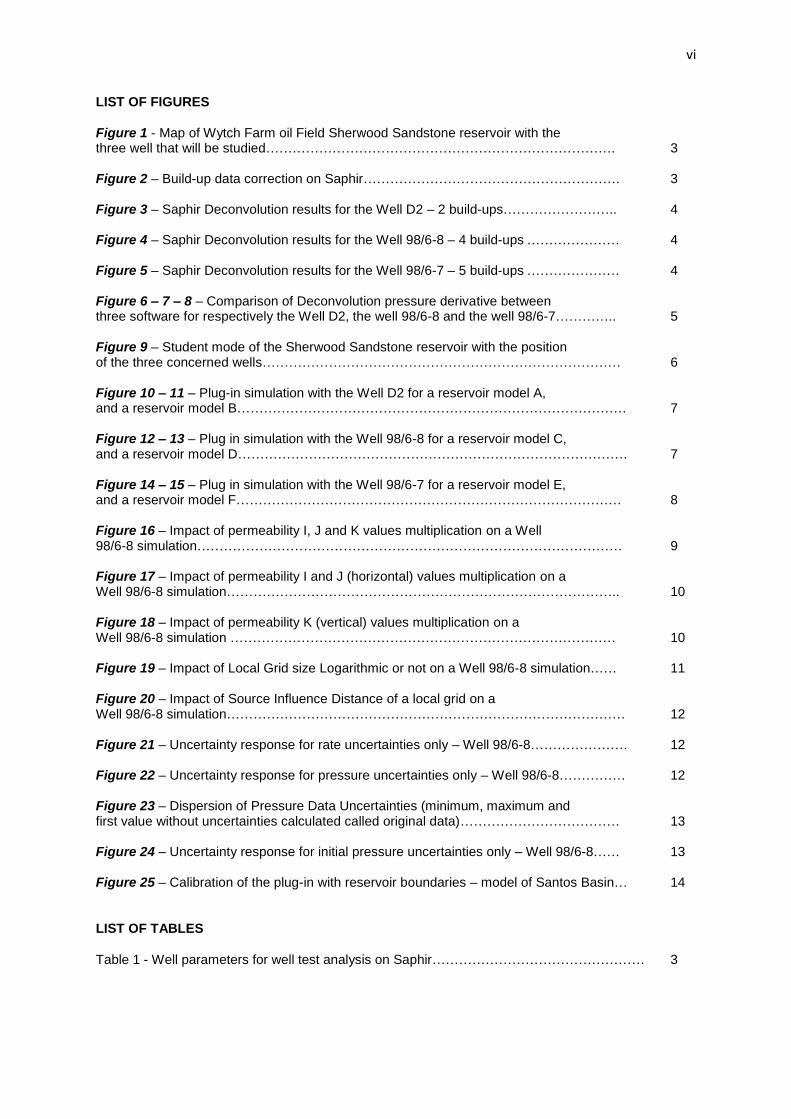
LIST OF FIGURES
Figure 1 - Map of Wytch Farm oil Field Sherwood Sandstone reservoir with the three well that will be studied……………………………………………………………………. 3 Figure 2 – Build-up data correction on Saphir…………………………………………………. 3 Figure 3 – Saphir Deconvolution results for the Well D2 – 2 build-ups…………………….. 4 Figure 4 – Saphir Deconvolution results for the Well 98/6-8 – 4 build-ups ………………… 4 Figure 5 – Saphir Deconvolution results for the Well 98/6-7 – 5 build-ups ………………… 4 Figure 6 – 7 – 8 – Comparison of Deconvolution pressure derivative between three software for respectively the Well D2, the well 98/6-8 and the well 98/6-7………….. 5 Figure 9 – Student mode of the Sherwood Sandstone reservoir with the position of the three concerned wells……………………………………………………………………… 6 Figure 10 – 11 – Plug-in simulation with the Well D2 for a reservoir model A, and a reservoir model B……………………………………………………………………………. 7 Figure 12 – 13 – Plug in simulation with the Well 98/6-8 for a reservoir model C, and a reservoir model D……………………………………………………………………………. 7 Figure 14 – 15 – Plug in simulation with the Well 98/6-7 for a reservoir model E, and a reservoir model F…………………………………………………………………………… 8 Figure 16 – Impact of permeability I, J and K values multiplication on a Well 98/6-8 simulation…………………………………………………………………………………… 9 Figure 17 – Impact of permeability I and J (horizontal) values multiplication on a Well 98/6-8 simulation…………………………………………………………………………….. 10 Figure 18 – Impact of permeability K (vertical) values multiplication on a Well 98/6-8 simulation …………………………………………………………………………… 10 Figure 19 – Impact of Local Grid size Logarithmic or not on a Well 98/6-8 simulation…… 11 Figure 20 – Impact of Source Influence Distance of a local grid on a Well 98/6-8 simulation……………………………………………………………………………… 12 Figure 21 – Uncertainty response for rate uncertainties only – Well 98/6-8…………………. 12 Figure 22 – Uncertainty response for pressure uncertainties only – Well 98/6-8…………… 12 Figure 23 – Dispersion of Pressure Data Uncertainties (minimum, maximum and first value without uncertainties calculated called original data)……………………………… 13 Figure 24 – Uncertainty response for initial pressure uncertainties only – Well 98/6-8…… 13 Figure 25 – Calibration of the plug-in with reservoir boundaries – model of Santos Basin… 14
LIST OF TABLES
Table 1 - Well parameters for well test analysis on Saphir………………………………………… 3
Verification and Improvement of the Reservoir Model with Well Test Analysis Thomas Rausch, Imperial College London and BG Group, Supervisors: Alain C. Gringarten (Imperial College London), Tim Whittle (Bg Group).
This paper was selected for presentation by an SPE program committee following review of information contained in an abstract submitted by the author(s). Contents of the paper have not been reviewed by the Society of Petroleum Engineers and are subject to correction by the author(s). The material does not necessar ily reflect any position of the Society of Petroleum Engineers, its officers, or members. Electronic reproduction, distribution, or storage of any part of this paper without the written consent of the Society of Petroleum Engineers is prohibited. Permission to reproduce in print is restricted to an abstract of not more than 300 words; illustrations may not be copied.
Abstract
Assessing well conditions, obtaining reservoir parameters and boundaries were possible for many years with Well Test
Analysis. In this work, a new way of using Well Test Analysis is presented. With the recent improvement of well testing
methods and tools like a stable deconvolution algorithm (Von Schroeter et al. 2001), well testing now provides interpretation
results with a high level of confidence. One main benefit of deconvolution is to give access to the actual radius of
investigation of the well, allowing the observation of boundaries and connectivities of a reservoir that cannot be observed on
individuals flow periods (Gringarten, 2010).
Reservoir modelling is also another important tool. After the integration of static and dynamic information, the reservoir
model allows to predict production performance and to calculate reserves. This paper presents the test of a new plug-in for
Petrel developed by BG Group and Blueback Reservoir Limited that allows petroleum engineers to validate a reservoir model
against actual well test. By comparing well test behaviours generated from the reservoir model with the deconvolved
derivatives of actual well tests. A quick visualisation of the possible mismatch or match between the two data is provided.
The plug-in was tested with some of the reservoir models created by Imperial College London students during the 2012-2013
group field development project which uses data from Wytch Farm. Well test data from three wells were used for validation
of the models.
As well test behaviors generated by the most models did not match actual well tests; different ways of improving the match
are investigated, with emphasis on the three main sources of uncertainties, well testing deconvolution, reservoir parameters
used to build the models and the use of the plug-in itself. Finally, suggestions for integrating the use of the plug-in in the
student work are provided.
Introduction Well Testing is a tool for reservoir evaluation and characterisation. It consists in a data acquisition process to understand and
to know better the properties and characteristics of a reservoir. During a well test, a transient pressure response is created by a
temporary change in production rate. This response is monitored during a certain amount of time (depending of the tests
objectives) and an analysis gives information on the reservoir and on the well (Bourdet, 2002).
Petroleum engineers use models in well test interpretation to define and predict the basic behaviour of the reservoir, its
connectivities, boundaries and also the near- wellbore effects.
Geophysicist, geological, and engineering information are used where possible in conjunction with the well test information
to build a reservoir model for production prevision. As data acquisition methods were improved, better identification methods
appeared. It had the direct consequences that more information with better accuracy can be extracted from well test data.
After the straight lines analysis in the 50s, the pressure type curve analysis, the type curves with independent variables in the
70s, the derivatives in the 80s, the interpretation methods became more consistent and more accurated.
More recently, the introduction of an effective algorithm for deconvolution by Schroeter et al. (2001) had upgraded the well
test analysis possibilities.
Deconvolution transforms a variable rate-pressure data into a constant rate initial drawdown with a duration equal to the total
time of the test. It produces directly the corresponding pressure derivatives which are normalized to a unit rate.

2 Verification and Improvement of the Reservoir Model with Well Test Analysis
It participated in increasing the data available for interpretation and allowed a better identification and interpretation of a
model: access of a bigger radius of investigation, boundaries and connectivities of the reservoir not visible in individual flow
periods can be now seen (Gringarten, 2010).
On the other hand, reservoir modelling is the construction of a model of a reservoir (Tyson, 2007). It is used to improve
estimations regarding the reserves and the production of a reservoir. With reservoir modelling software products, the
development options of the field can be studied before investments. Commercially available since 1998, Petrel is a
Schlumberger software application to gather oil reservoir data from multiple sources. Interpreting seismic data, building
reservoir models for simulation and designing development strategiesto maximise reservoir exploitation are the three main
objectives of this tool. The software is closely linked to Eclipse and FrontSim. They are both 3D reservoir simulator. Eclipse
is also a Schlumberger product, and Fronstim is a Petrofaq product.
Blueback Reservoir and BG Group collaborated in 2012 to develop a plug-in of Petrel integrating well test analysis directly
in the process of reservoir modelling which contributes to generate reservoir models more accurately. It is a new technology
and it allows comparison between well test behaviours generated from the reservoir model with the deconvolved derivatives
from actual well tests. The plug-in shows the mismatch quickly, it is a verification tool. It does not improve the reservoir
model, but it can tell that the reservoir model is not consistent with the well test analysis information. As the geometry and
the connectivities of a reservoir are established with the static model, the plug-in is used after the static reservoir modelling
process made by geoscientists. Petroleum engineers use well test information and dynamic information to refine the model by
adjusting model parameters. The final result is an improvement of reservoir modelling for forecasting and development
decision making.
Imperial College London proposes every year a project to its Petroleum students. They have to develop a complete field
development plan for the Wytch Farm oil field. It is the largest onshore oilfield in Western Europe located in Dorset,
Southern England. Students’ teams have to create a static, then a dynamic model, analyse well tests data, and propose a
suitable strategy for the field development.
The global aim of the present study is to use the plug-in to verify the validity of the students’ reservoir models developed
during phase 1 and phase 2 of the group project. The phase 1 consisted in the appraisal, the characterisation and modelling of
the reservoir. Students had to produce a geological model of the field with a 3D geocellular realisation of the reservoir. The
objective was to estimate the Stock Tank Oil Initially In Place (STOIIP) value and reserves. The phase 2 focused in a
construction of a simple upscaled simulation model after finalising the 3D static models and in using it to investigate a how
to optimise the production in a simple development scheme.
If a mismatch is observed, the second objective is to propose ways to improve them. In a first part of the report, well test data
from three wells are analysed and used. In a second part, the plug-in is tested and a tutorial is provided in order to guide
students or professional who want to use it. The plug-in would allow students to adjust directly their static model using the
well test analyses in order to have a more realistic dynamic model. In a third and last part, the uncertainties of the project are
discussed. Recommendations for future users and conclusion are written at the end of the report.
Well Test Analysis of the three wells
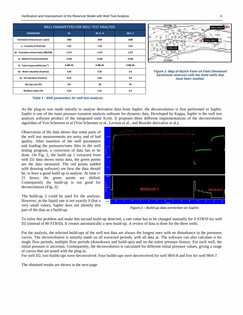
The first main part of the study is the analysis of the well test data of three wells (the well D2, 98/6-7 and 98/6-8). The main
well parameters were given in the brief of the student project and are summarised in the Table 1. A map of the reservoir is
also provided with the position of the three wells (Fig. 1).
Verification and Improvement of the Reservoir Model with Well Test Analysis 3
As the plug-in was made initially to analyse derivative data from Saphir, the deconvolution is first performed in Saphir.
Saphir is one of the main pressure transient analysis software for dynamic data. Developed by Kappa, Saphir is the well test
analysis software product of the integrated suite Ecrin. It proposes three different implementations of the deconvolution
algorithm of Von Schoreter et al (Von Schroeter et al., Levitan et al., and Bourdet derivative et al.).
Observation of the data shows that some parts of
the well test measurements are noisy and of bad
quality. After insertion of the well parameters
and loading the pressures/rates files in the well
testing program, a correction of data has to be
done. On Fig. 2, the build up 1 extracted from
well D2 data shows noisy data, the green points
are the data measured. The red points (added
with drawing software) are how the data should
be, to have a good build up to analyse. At time t=
21 hours, the green points are shifted.
Consequently the build-up is not good for
deconvolution (Fig. 2).
The build-up 2 could be used for the analysis.
However, as the liquid rate is not exactly 0 (but a
very small value), Saphir does not identify this
part of the data as a build-up.
To solve this problem and make this second build-up detected, a rate value has to be changed manually for 0 STB/D for well
D2 (instead of 80 STB/D). It creates automatically a new build-up. A review of data is done for the three wells.
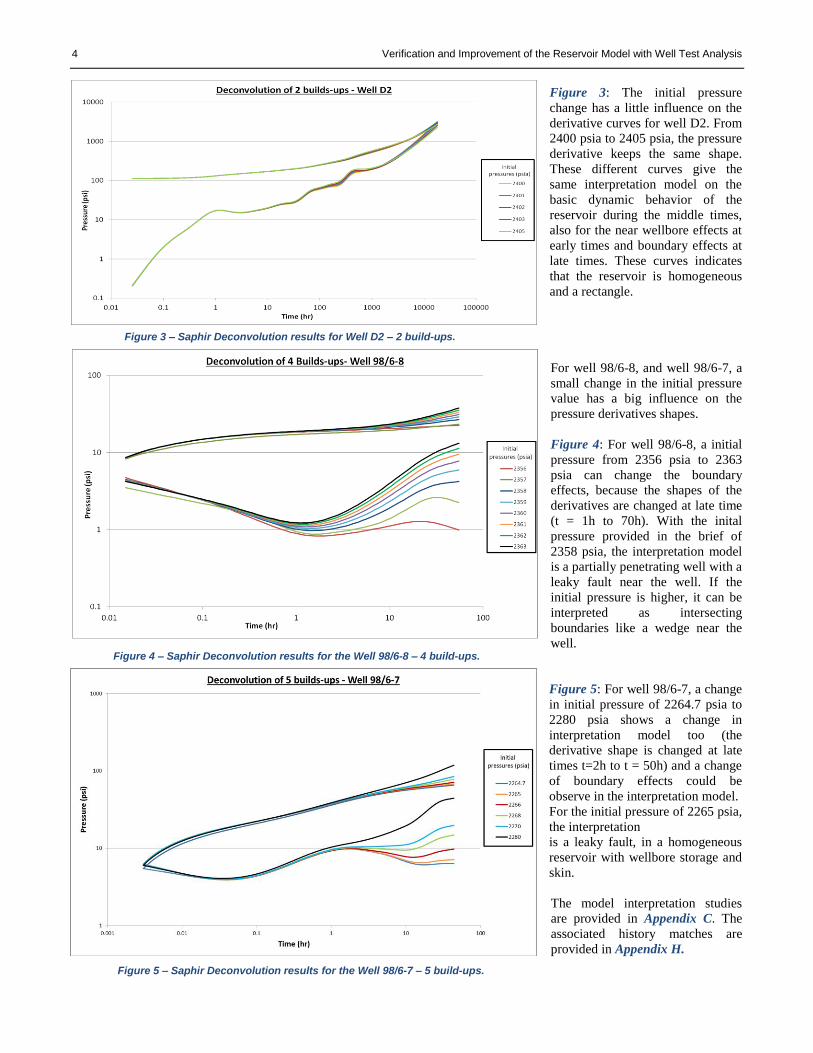
For the analysis, the selected build-ups of the well test data are always the longest ones with no disturbance in the pressures
curves. The deconvolution is initially made on all extracted periods, with all data at. The software can also calculate it for
single flow periods, multiple flow periods (drawdrawn and build-ups) and on the entire pressure history. For each well, the
initial pressure is uncertain. Consequently, the deconvolution is calculated for different initial pressure values, giving a range
of curves that are tested with the plug-in.
For well D2, two builds-ups were deconvolved. Four builds-ups were deconvolved for well 98/6-8 and five for well 98/6-7.
The obtained results are shown in the next page.
9.48E-06
0.4
0.6
95
0.4
98/ 6 -7
2268
1.03
1.277
0.1960.196
1.03 1.03μ - Viscosity of Fluid (cp)
Wellbore radius (ft)
0.56 0.66
0.24 0.51
Sw - Water saturation (fraction) 0.44 0.34
Net pay zone (ft) 114 58
WELL PARAMETERS FOR WELL TEST ANALYSIS
So - Oil saturation (fraction)
Bo - Formation volume factor (RB/STB) 1.277 1.277
Ct - Total compressibility (psi-1) 9.48E-06 9.48E-06
D2 98 / 6 - 8PARAMETERS
Estimated initial pressure (psia) 2403 2358
ф - (Matrix) Porosity (fraction) 0.194
Figure 1- Map of Wytch Farm oil Field Sherwood Sandstone reservoir with the three wells that
have been studied.
Table 1 - Well parameters for well test analysis.
Figure 2 – Build-up data correction on Saphir.
4 Verification and Improvement of the Reservoir Model with Well Test Analysis
Figure 3: The initial pressure
change has a little influence on the
derivative curves for well D2. From
2400 psia to 2405 psia, the pressure
derivative keeps the same shape.
These different curves give the
same interpretation model on the
basic dynamic behavior of the
reservoir during the middle times,
also for the near wellbore effects at
early times and boundary effects at
late times. These curves indicates
that the reservoir is homogeneous
and a rectangle.
For well 98/6-8, and well 98/6-7, a
small change in the initial pressure
value has a big influence on the
pressure derivatives shapes.
Figure 4: For well 98/6-8, a initial
pressure from 2356 psia to 2363
psia can change the boundary
effects, because the shapes of the
derivatives are changed at late time
(t = 1h to 70h). With the inital
pressure provided in the brief of
2358 psia, the interpretation model
is a partially penetrating well with a
leaky fault near the well. If the
initial pressure is higher, it can be
interpreted as intersecting
boundaries like a wedge near the
well.
Figure 5: For well 98/6-7, a change
in initial pressure of 2264.7 psia to
2280 psia shows a change in
interpretation model too (the
derivative shape is changed at late
times t=2h to t = 50h) and a change
of boundary effects could be
observe in the interpretation model.
For the initial pressure of 2265 psia,
the interpretation
is a leaky fault, in a homogeneous
reservoir with wellbore storage and
skin.
The model interpretation studies
are provided in Appendix C. The
associated history matches are
provided in Appendix H.
Figure 4 – Saphir Deconvolution results for the Well 98/6-8 – 4 build-ups.
Figure 3 – Saphir Deconvolution results for Well D2 – 2 build-ups.
Figure 5 – Saphir Deconvolution results for the Well 98/6-7 – 5 build-ups.
Verification and Improvement of the Reservoir Model with Well Test Analysis 5
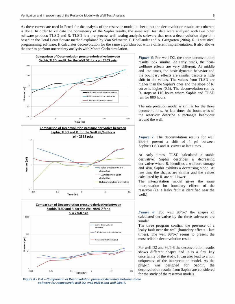
As these curves are used in Petrel for the analysis of the reservoir model, a check that the deconvolution results are coherent
is done. In order to validate the consistency of the Saphir results, the same well test data were analysed with two other
software product: TLSD and R. TLSD is a pre-process well testing analysis software that uses a deconvolution algorithm
based on the Total Least Square method explained by Von Schroeter, T. Hoellander and A. Gringarten (2004). R. is statistical
programming software. It calculates deconvolution for the same algorithm but with a different implementation. It also allows
the user to perform uncertainty analysis with Monte Carlo simulation.
Figure 6: For well D2, the three deconvolution
results look similar. At early times, the near-
wellbore effects are very different. At middle
and late times, the basic dynamic behavior and
the boundary effects are similar despite a little
shift in the values. The values from TLSD are
higher than the Saphir's ones and the slope of R.
curve is higher (0.5). The deconvolution run by
R. stops at 110 hours where Saphir and TLSD
run for 880 hours.
The interpretation model is similar for the three
deconvolutions. At late times the boundaries of
the reservoir describe a rectangle beahviour
around the well.
Figure 7: The deconvolution results for well
98/6-8 present a shift of 4 psi between
Saphir/TLSD and R. curves at late times.
At early times, TLSD calculated a stable
derivative. Saphir describes a decreasing
derivative where R. identifies a wellbore storage
and skin, Saphir exhibits a decreasing slope. At
late time the shapes are similar and the values
calculated by R. are still lower.
The interpretation model gives the same
interpretation for boundary effects of the
reservoir (i.e. a leaky fault is identified near the
well.)
Figure 8: For well 98/6-7 the shapes of
calculated derivative by the three softwares are
similar.
The three program confirm the presence of a
leaky fault near the well (boundary effects - late
times). The well 98/6-7 seems to present the
most reliable deconvolution result.
For well D2 and 98/6-8 the deconvolution results
shows different shapes and it is a first key
uncertainty of the study. It can also lead to a non
uniqueness of the interpretation model. As the
plug-in was designed for Saphir, the
deconvolution results from Saphir are considered
for the study of the reservoir models.
Figure 6 - 7- 8 – Comparison of Deconvolution pressure derivative between three software for respectively well D2, well 98/6-8 and well 98/6-7.

6 Verification and Improvement of the Reservoir Model with Well Test Analysis
Analysis of the reservoir models with the plug-in
With the deconvolution done, the pressure and pressure derivatives values calculated by Saphir can be used in Petrel to
analysed the reservoir model with the help of the Blueback Toolbox, which is a suite of plug-ins for Petrel developed by
Bluback Reservoir Limited and BG Group.
It contains seven modules (geology, seismic inversion, geophysics, project management, reservoir engineering, seismic
reservoir characterization, and well test simulation/ quality control) and this project focusses in the Well Test Simulation
(WTS) & Quality Control (QC) module.
The WTS & QC plug-in was built to compare the well pressure test data (from Saphir) to the bottom-hole pressure calculated
by an Eclipse model (created from a reservoir model).
The advantages of the plug-in can be explained in a real-scale oil and gas company context. An engineer has a well test of a
reservoir well. The geologist built a static model of this reservoir. The plug-in allows comparing the measured data (the
actual well test data) with the well test behaviours generated from the reservoir model. The engineer and the geologist can
observe a mismatch and can adjust together the model parameters and the model itself (i.e. the faults, or the connectivities of
the reservoir) to make match both data.
Engineers can refine the model with the dynamic model. The plug-in acts like a real connection between the static and the
dynamic model and between engineers and geologists. They can decide as a team what parameters to adjust. It also
participates in unlocking the information of well tests, and consequently in improving models accuracy and forecasting for
future development strategies.
This project was to check the validity of students’ reservoir models with the help of the plug-in and a tutorial is provided in
Appendix B.
The main steps of its use are summarized in
the report. After importing the derivative data
of a well from a well-testing software in
Petrel, the perforations of this well has to be
confirmed for the plug-in. Then, a local grid
refinement has to be created around this well
in order to increase the accuracy of the well
zone.
Later, a development strategy is created with
a specific well rate production control rule
and a derivative timestep rule. A simulation
case is run using Eclipse with this
development strategy, some properties of the
reservoir model and the local grid.
This simulation case creates well test
behaviors (pressure and derivative curves
from the reservoir model), and the plug-in
shows on the same graph the derivative data
imported from Saphir at the beginning.
To run an analysis of a well on the plug-in,
The following parameters are needed:
- A well
- Perforations of this well
- Permeability I, J (horizontal) and K (vertical)
- Porosity of the model
- Net To Gross ratio
- Fluid and rock properties (drainage relative permeability, black oil fluid model with initial conditions, rock
compaction).
All students modelised the same oil field with Petrel. Logically, the reservoir models are the same in apparence for all groups
(Fig. 9) however the parameters, reservoir properties values and the settings change between all models because the different
parameters were chosen by students. Nevertheless, the obtained results are all similar and similar shapes can be recognised
between all students models. No match was observed for any model and any well. The two best results for each well are
presented in the report. On the figures, four curves are represented. Two are coming from the Saphir deconvolution (called
derivative data, which are pressure and pressure derivative deconvolved curves), and the two others are generated by the
plug-in with the reservoir model (called case, which are simulated pressure and pressure derivative curves).
Figure 9 – Student model of the Sherwood Sandtone reservoir with the position of the three concerned wells.
Verification and Improvement of the Reservoir Model with Well Test Analysis 7
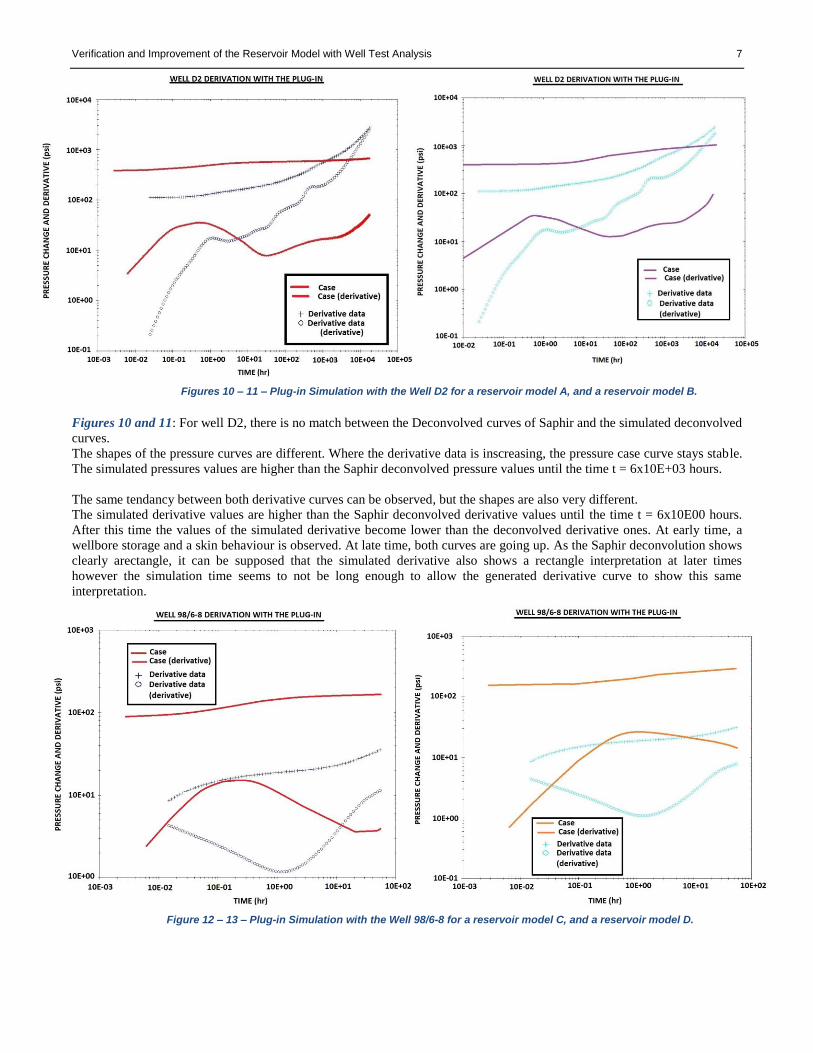
Figures 10 and 11: For well D2, there is no match between the Deconvolved curves of Saphir and the simulated deconvolved
curves.
The shapes of the pressure curves are different. Where the derivative data is inscreasing, the pressure case curve stays stable.
The simulated pressures values are higher than the Saphir deconvolved pressure values until the time t = 6x10E+03 hours.
The same tendancy between both derivative curves can be observed, but the shapes are also very different.
The simulated derivative values are higher than the Saphir deconvolved derivative values until the time t = 6x10E00 hours.
After this time the values of the simulated derivative become lower than the deconvolved derivative ones. At early time, a
wellbore storage and a skin behaviour is observed. At late time, both curves are going up. As the Saphir deconvolution shows
clearly arectangle, it can be supposed that the simulated derivative also shows a rectangle interpretation at later times
however the simulation time seems to not be long enough to allow the generated derivative curve to show this same
interpretation.
Figures 10 – 11 – Plug-in Simulation with the Well D2 for a reservoir model A, and a reservoir model B.
Figure 12 – 13 – Plug-in Simulation with the Well 98/6-8 for a reservoir model C, and a reservoir model D.
8 Verification and Improvement of the Reservoir Model with Well Test Analysis
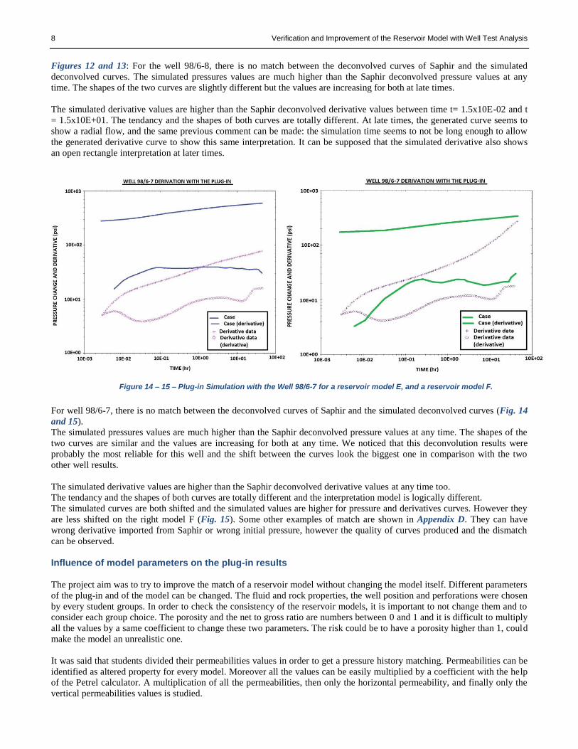
Figures 12 and 13: For the well 98/6-8, there is no match between the deconvolved curves of Saphir and the simulated
deconvolved curves. The simulated pressures values are much higher than the Saphir deconvolved pressure values at any
time. The shapes of the two curves are slightly different but the values are increasing for both at late times.
The simulated derivative values are higher than the Saphir deconvolved derivative values between time t= 1.5x10E-02 and t
= 1.5x10E+01. The tendancy and the shapes of both curves are totally different. At late times, the generated curve seems to
show a radial flow, and the same previous comment can be made: the simulation time seems to not be long enough to allow
the generated derivative curve to show this same interpretation. It can be supposed that the simulated derivative also shows
an open rectangle interpretation at later times.
For well 98/6-7, there is no match between the deconvolved curves of Saphir and the simulated deconvolved curves (Fig. 14
and 15).
The simulated pressures values are much higher than the Saphir deconvolved pressure values at any time. The shapes of the
two curves are similar and the values are increasing for both at any time. We noticed that this deconvolution results were
probably the most reliable for this well and the shift between the curves look the biggest one in comparison with the two
other well results.
The simulated derivative values are higher than the Saphir deconvolved derivative values at any time too.
The tendancy and the shapes of both curves are totally different and the interpretation model is logically different.
The simulated curves are both shifted and the simulated values are higher for pressure and derivatives curves. However they
are less shifted on the right model F (Fig. 15). Some other examples of match are shown in Appendix D. They can have
wrong derivative imported from Saphir or wrong initial pressure, however the quality of curves produced and the dismatch
can be observed.
Influence of model parameters on the plug-in results
The project aim was to try to improve the match of a reservoir model without changing the model itself. Different parameters
of the plug-in and of the model can be changed. The fluid and rock properties, the well position and perforations were chosen
by every student groups. In order to check the consistency of the reservoir models, it is important to not change them and to
consider each group choice. The porosity and the net to gross ratio are numbers between 0 and 1 and it is difficult to multiply
all the values by a same coefficient to change these two parameters. The risk could be to have a porosity higher than 1, could
make the model an unrealistic one.
It was said that students divided their permeabilities values in order to get a pressure history matching. Permeabilities can be
identified as altered property for every model. Moreover all the values can be easily multiplied by a coefficient with the help
of the Petrel calculator. A multiplication of all the permeabilities, then only the horizontal permeability, and finally only the
vertical permeabilities values is studied.
Figure 14 – 15 – Plug-in Simulation with the Well 98/6-7 for a reservoir model E, and a reservoir model F.
Verification and Improvement of the Reservoir Model with Well Test Analysis 9
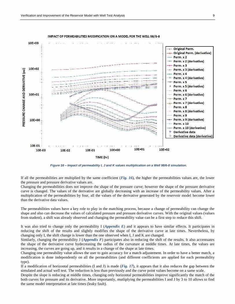
If all the permeabilities are multiplied by the same coefficient (Fig. 16), the higher the permeabilities values are, the lower
the pressure and pressure derivative values are.
Changing the permeabilities does not improve the shape of the pressure curve; however the shape of the pressure derivative
curve is changed. The values of the derivative are globally decreasing with an increase of the permeability values. After a
multiplication of the permeabilities by four, all the values of the derivative generated by the reservoir model become lower
than the derivative data values.
The permeabilities values have a key role to play in the matching process, because a change of permeability can change the
shape and also can decrease the values of calculated pressure and pressure derivative curves. With the original values (values
from student), a shift was already observed and changing the permeability value can be a first step to reduce this shift.
It was also tried to change only the permeability I (Appendix E) and it appears to have similar effects. It participates in
reducing the shift of the results and slightly modifies the shape of the derivative curve at late times. Nevertheless, by
changing only I, the shift change is lower than the one observed when I, J and K are changed.
Similarly, changing the permeability J (Appendix F) participates also in reducing the shift of the results. It also accentuates
the shape of the derivative curve bydecreasing the radius of the curvature at middle times. At late times, the values are
increasing, the curves are going up, and it results in a change of the shape at late times.
Changing one permeability value allows the user to gain accuracy for a match adjustement. In order to have a better match, a
modification is done independently on all the permeabilities (and different coefficients are applied for each permeability
type).
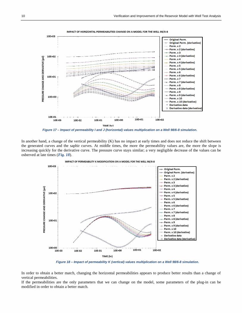
If a modification of horizontal permeabilities (I and J) is made (Fig. 17), it appears that it also reduces the gap between the
simulated and actual well test. The reduction is less than previously and the curve point values become on a same scale.
Despite the slope is reducing at middle times, changing only horizontal permeabilities improve significantly the match of the
both curves for pressure and its derivative. More importantly, mutliplying the permeabilities I and J by 3 to 10 allows to find
the same model interpretation at late times (leaky fault).
Figure 16 – Impact of permeability I, J and K values multiplication on a Well 98/6-8 simulation.
10 Verification and Improvement of the Reservoir Model with Well Test Analysis
In another hand, a change of the vertical permeability (K) has no impact at early times and does not reduce the shift between
the generated curves and the saphir curves. At middle times, the more the permeability values are, the more the slope is
increasing quickly for the derivative curve. The pressure curve stays similar; a very negligible decrease of the values can be
osberved at late times (Fig. 18).
In order to obtain a better match, changing the horizontal permeabilities appears to produce better results than a change of
vertical permeabilities.
If the permeabilities are the only parameters that we can change on the model, some parameters of the plug-in can be
modified in order to obtain a better match.
Figure 17 – Impact of permeability I and J (horizontal) values multiplication on a Well 98/6-8 simulation.
Figure 18 – Impact of permeability K (vertical) values multiplication on a Well 98/6-8 simulation.
Verification and Improvement of the Reservoir Model with Well Test Analysis 11
As a local grid size has to be settled around the well zone, the grid size and the source influence distance are two parameters
defined by the plug-in.
Three inputs can be modified when a local grid is created: the size of the local grid (expressed in blocks of 3 dimensions
AxBxC), the source influence distance (expressed in metres), and the fact that the local grid can be logarithmic or not.
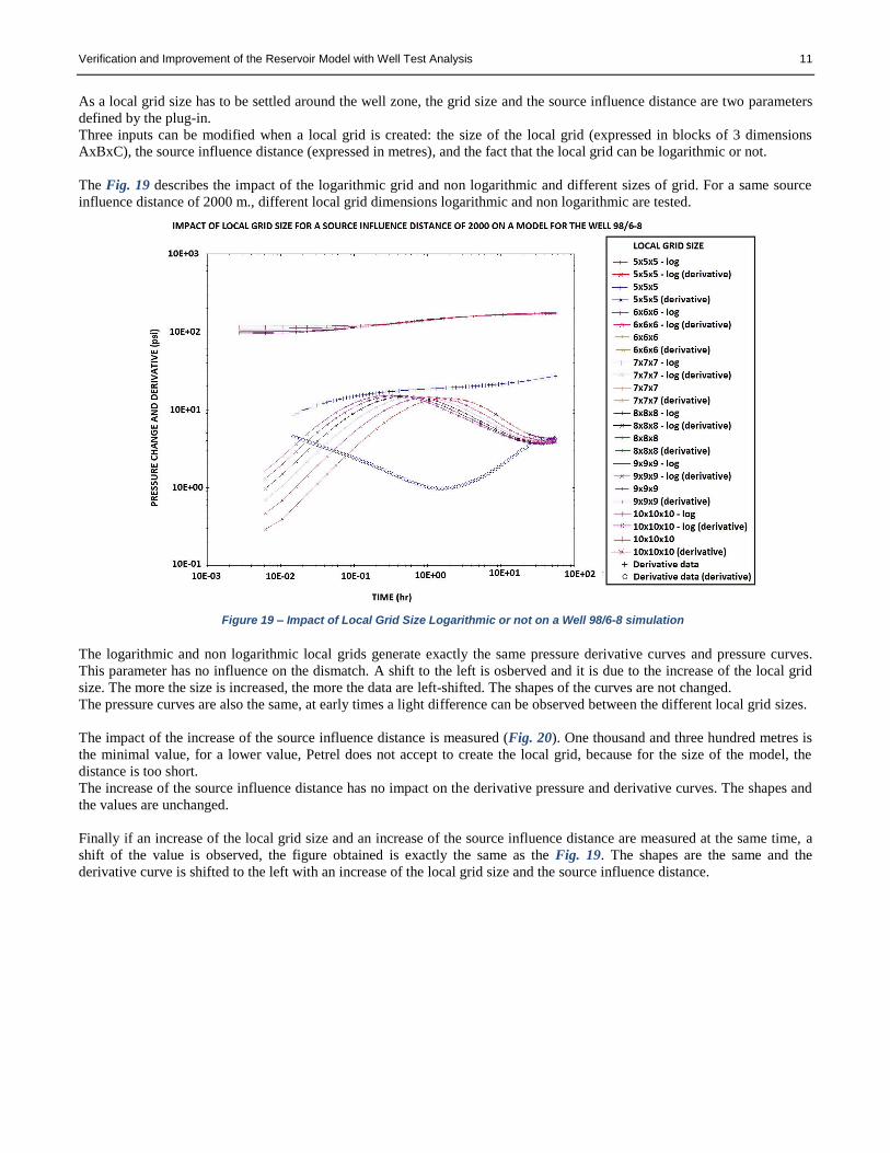
The Fig. 19 describes the impact of the logarithmic grid and non logarithmic and different sizes of grid. For a same source
influence distance of 2000 m., different local grid dimensions logarithmic and non logarithmic are tested.
The logarithmic and non logarithmic local grids generate exactly the same pressure derivative curves and pressure curves.
This parameter has no influence on the dismatch. A shift to the left is osberved and it is due to the increase of the local grid
size. The more the size is increased, the more the data are left-shifted. The shapes of the curves are not changed.
The pressure curves are also the same, at early times a light difference can be observed between the different local grid sizes.
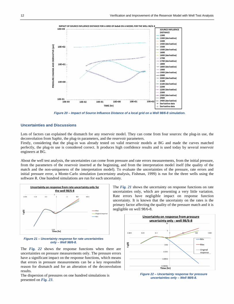
The impact of the increase of the source influence distance is measured (Fig. 20). One thousand and three hundred metres is
the minimal value, for a lower value, Petrel does not accept to create the local grid, because for the size of the model, the
distance is too short.
The increase of the source influence distance has no impact on the derivative pressure and derivative curves. The shapes and
the values are unchanged.
Finally if an increase of the local grid size and an increase of the source influence distance are measured at the same time, a
shift of the value is observed, the figure obtained is exactly the same as the Fig. 19. The shapes are the same and the
derivative curve is shifted to the left with an increase of the local grid size and the source influence distance.
Figure 19 – Impact of Local Grid Size Logarithmic or not on a Well 98/6-8 simulation
12 Verification and Improvement of the Reservoir Model with Well Test Analysis
Uncertainties and Discussions
Lots of factors can explained the dismatch for any reservoir model. They can come from four sources: the plug-in use, the
deconvolution from Saphir, the plug-in parameters, and the reservoir parameters.
Firstly, considering that the plug-in was already tested on valid reservoir models at BG and made the curves matched
perfectly, the plug-in use is considered correct. It produces high confidence results and is used today by several reservoir
engineers at BG.
About the well test analysis, the uncertainties can come from pressure and rate errors measurements, from the initial pressure,
from the parameters of the reservoir inserted at the beginning, and from the interpretation model itself (the quality of the
match and the non-uniqueness of the interpretation model). To evaluate the uncertainties of the pressure, rate errors and
initial pressure error, a Monte-Carlo simulation (uncertainty analysis, Fishman, 1999) is run for the three wells using the
software R. One hundred simulations are run for each uncertainty.
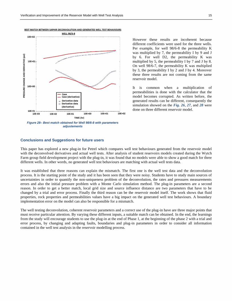
The Fig. 21 shows the uncertainty on response functions on rate
uncertainties only, which are presenting a very little variation.
Rate errors have negligible impact on response function
uncertainty. It is known that the uncertainty on the rates is the
primary factor affecting the quality of the pressure match and it is
negligible on well 98/6-8.
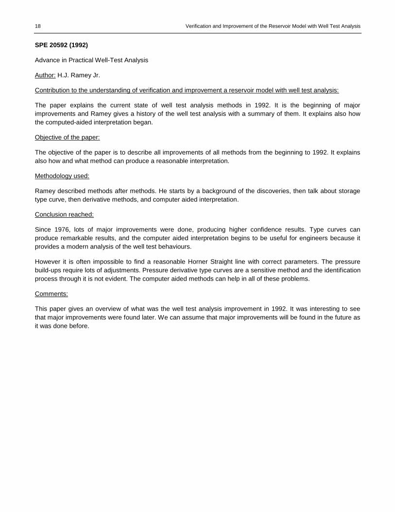
The Fig. 22 shows the response functions when there are
uncertainties on pressure measurements only. The pressure errors
have a significant impact on the response functions, which means
that errors in pressure measurements can be a key responsible
reason for dismatch and for an alteration of the deconvolution
results.
The dispersion of pressures on one hundred simulations is
presented on Fig. 23.
Figure 20 – Impact of Source Influence Distance of a local grid on a Well 98/6-8 simulation.
Figure 21 – Uncertainty response for rate uncertainties only – Well 98/6-8.
Figure 22 – Uncertainty response for pressure
uncertainties only – Well 98/6-8.

Verification and Improvement of the Reservoir Model with Well Test Analysis 13
The Fig. 24 shows the effects of the initial pressure uncertainty on the response function. We knew that it was important
because a small change in the value had a big impact on the deconvolution curve in Saphir. This figure confirms it, and
uncertainty in initial pressure can be responsible for the behaviour of the pressure derivative at late times (Cumming et al. ,
2013). Consequently the dismatch at late times can be justified by error in initial pressure estimation. The well 98/6-8 was
shown because it is the well that shows highest uncertainties. The uncertainties of the two other wells are acceptable (so are
not analysed in this report) and are provided in Appendix G.
It was also noticed at the beginning of the report that according to the algorithm, the deconvolution could have a different
shape. As only the Saphir deconvolution was analysed in the plug-in, another algorithm implementation might match better.
It was known that the data were noisy and have measurements errors at the beginning. The uncertainty analysis justifies the
implication of the Saphir deconvolution in the dismatch of the pressure and derivative curves.
However, it is probably the reservoir model parameters that have the important impact on the dismatch. First of all, it was
observed that some wells of models have their perforations containing a water zone. The perforation depths can alter the final
results and can change the shape of the model response generated. It can be explained probably by a mistake of unit
conversion (TVDSS and MD). Some groups also forgot to consider completion of the wells. Consequently, the flow is
observed only near the borehole, changing it in a spherical flow. The students underestimated the real damages brought by
the completion around the well zones, changing also the generated model response.
Secondly, every group chose their own parameters and could not follow the parameters indicated in the brief. Indeed, one
main aim of the Wytch Farm project was to estimate a STOIIP value.
𝑆𝑇𝑂𝐼𝐼𝑃 =𝐺𝑅𝑉 × 𝑁𝑇𝐺 × ϕ × (1 − Sw)
𝐵𝑜
Where GRV is the Gross Rock Volume of the reservoir. It is defined by the rock properties, like NTG, the Net To Gross
ratio. Φ is the average porosity, and it is also defined by the rock properties. It was upscaled from one cell around the well by
the geologists. Sw is the water saturation, and Bo is the oil formation volume factor. These two inputs are defined by the fluid
properties.
As students generated their own fluid and rock properties, they adapted the values, in order to increase or decrease their
STOIIP value to provide a realistic value or at least a close value to the other groups. Moreover, the process of determining
the porosity is very uncertain and the values can be wrong.
Thirdly, it was presented that the permeability values have also a big influence on the shape and on the values of the
generated model responses. In order to have a pressure history matching, students confessed having divided their
permeabilities values. The pressure and pressure derivatives curves are also altered by this modification. And the shift
between the actual well test behaviours and the generated curves is explained by the permeability change.
Fourthly, every group considered the boundaries and the position of faults in their models. However some positions of the
faults were wrong and it can be seen on the model response. The shift between the generated derivative curve and the Saphir
Figure 23 – Dispersion of Pressure data uncertainties (Minimum, Maximum and first value without uncertaintiescalculated called original data).
Figure 24 – Uncertainty response for initial pressure
uncertainties only – Well 98/6-8.

14 Verification and Improvement of the Reservoir Model with Well Test Analysis
derivative curve and also between the generated pressure and Saphir pressure curve can be explained by a fault distance error.
This comment points out one use of the plug-in.
We assume that all the reservoir parameters and the Saphir deconvolution are correct and present no uncertainties. A
reservoir model is created and analysed with the plug-in. A dismatch is observed. The implementation of a closer fault per
example will change the generated well test behaviours (Fig. 25). The reservoir model can be analysed again with the plug-in
and a better match can be observed. In other words, a trial and error process has to be settled in order to take the advantages
of the well test analysis for reservoir modeling.
The last point is about the saving system of the Wytch Farm project. Every group had a space on a servor to save their data
and their reservoir models. Some groups saved everything on the share space. If two members are using the model at the
same time and save an input on it, the model becomes corrupted. It can be impossible to run simulation (Eclipse detects
errors in the grid of the model) or the results can be unrealistic. Some other groups saved their models on their computer to
run the simulations. In this case, we analysed uncomplete models because we did not have access to these data (the plug-in
license was only available on one computer).
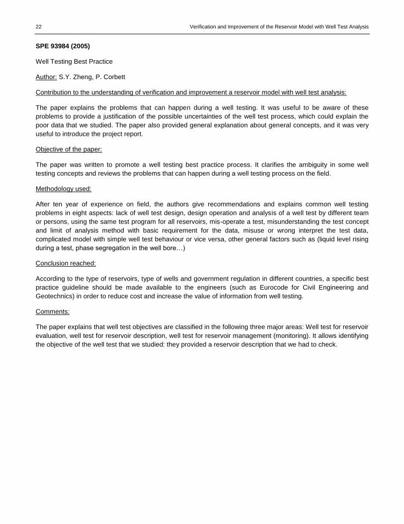
Finally, by multiplicating the permeabilities I, J and K by certain coefficients and by using a certain local grid with an
associated source influence distance, we can improve the match of both results for the three wells (Fig. 26, 27 and 28).
Figure 26 and 27– Best match obtained for Well D2 and 98/6-7with parameters adjustements
Figure 25 – Calibration of the plug-in with reservoir boundaries. Source: BG Group, presentation for the chief executive innovation award, 2012.
Verification and Improvement of the Reservoir Model with Well Test Analysis 15
However these results are incoherent because
different coefficients were used for the three wells.
Per example, for well 98/6-8 the permeability K
was multiplied by 7, the permeability I by 9 and J
by 6. For well D2, the permeability K was
multiplied by 5, the permeability I by 7 and J by 8.
On well 98/6-7, the permeability K was multiplied
by 3, the permeability I by 2 and J by 4. Moreover
these three results are not coming from the same
reservoir model.
It is common when a multiplication of
permeabilities is done with the calculator that the
model becomes corrupted. As written before, the
generated results can be different, consequently the
simulation showed on the Fig. 26, 27, and 28 were
done on three different reservoir model.
Conclusions and Suggestions for future users
This paper has explored a new plug-in for Petrel which compares well test behaviours generated from the reservoir model
with the deconvolved derivatives and actual well tests. After analysis of student reservoirs models created during the Wytch
Farm group field development project with the plug-in, it was found that no models were able to show a good match for three
different wells. In other words, no generated well test behaviours are matching with actual well tests data.
It was established that three reasons can explain the mismatch. The first one is the well test data and the deconvolution
process. It is the starting point of the study and it has been seen that they were noisy. Students have to study main sources of
uncertainties in order to quantify the non-uniqueness problem of the deconvolution, the rates and pressures measurements
errors and also the initial pressure problem with a Monte Carlo simulation method. The plug-in parameters are a second
reason. In order to get a better match, local grid size and source influence distance are two parameters that have to be
changed by a trial and error process. Finally the third reason can be the reservoir model itself. The work shows that fluid
properties, rock properties and permeabilities values have a big impact on the generated well test behaviours. A boundary
implementation error on the model can also be responsible for a mismatch.
The well testing deconvolution, coherent reservoir parameters and a correct use of the plug-in have are three major points that
must receive particular attention. By varying these different inputs, a suitable match can be obtained. In the end, the learnings
from the study will encourage students to use the plug-in at the end of Phase 1, at the beginning of the phase 2 with a trial and
error process, by changing and adapting faults, boundaries and plug-in parameters in order to consider all information
contained in the well test analysis in the reservoir modelling process.
Figure 28– Best match obtained for Well 98/6-8 with parameters
adjustements

16 Verification and Improvement of the Reservoir Model with Well Test Analysis
Nomenclature
Name Description Dimension, units (SI)
𝐶𝑡
Total compressibility
𝐿. 𝑇2. 𝑀−1
𝐵𝑜 Formation Volume Factor of Oil 𝐿3. 𝐿−3
𝜙 Matrix porosity 𝑁𝑜 𝑢𝑛𝑖𝑡
𝑁𝑇𝐺 Net To Gross ratio 𝑁𝑜 𝑢𝑛𝑖𝑡
𝑆𝑜 Oil Saturation 𝑁𝑜 𝑢𝑛𝑖𝑡
𝐼, 𝐽, 𝐾 Permeabilities 𝐿2
𝑃𝑉 Pore Volume 𝐿3
𝑡 Time 𝑇
𝜇 Viscosity of the fluid 𝑀. 𝐿−1. 𝑇−1
𝑆𝑤 Water Saturation 𝑁𝑜 𝑢𝑛𝑖𝑡
References
Anraku, T., Horne, R. N. 1993. Discrimination between Reservoir Models in Well-Test Analysis. Paper SPE 26426 presented
at the 1993 SPE Annual Technical Conference and Exhibition, Houston, Oct. 3-6.
Armudo, C., Turner, J., Frewin, J., Kgogo, T.C., Gringarten, A.C. 2006. Integration of Well-Test Deconvolution Analysis
and Detailed Reservoir Modelling in 3D Sismic Data Interpretation: A Case Study. Paper SPE prepared for
presentation at the 2006 SPE Europec/EAGE Annual Conference and Exhibition, Vienna, June 12-15.
Azi A. C., Whittle, T., Gringarten, A.C. 2008. Evaluation of Confidence Intervals in Well Test Interpretation Results. Paper
SPE 113888 prepared for presentation at the 2008 SPE Europec/EAGE Annual Conference and Exhibition,
Rome, June 9-12.
Bourdet, D. 2002. Well Test Analysis: The Use of Advanced Interpretation Models, first edition, Elsevier Science B.V.,
Amsterdam, 205.
Cumming, J. A., Wooff, D.A., Whittle, T., Crossman R.J., Gringarten, A.C. 2013. Assessing the Non-Uniqueness of the Well
Test Interpretation Model Using Deconvolution. Paper SPE 164870 prepared for presentation at the EAGE
Annual Conference and Exhibition incorporating SPE Europec, London, June 10-13.
Gringarten, A. C.. 2006. From Straight Lines to Deconvolution: The Evolution of the State of the Art in Well Test Analysis.
Paper SPE 102079 presented at the 2006 SPE Annual Technical Conference and Exhibition, San Antonio,
Sept. 24-27.
Gringarten, A.C. 2010. Practical Use of Well Test Deconvolution. Paper SPE presented at the 2010 Annual Technical
Conference and Exhibition, Florence, Sept. 20-22.
Gringarten, A. C. 2012. Well Test Analysis in Practice. Thewayahead: vol 8. no. 2.
Horne, R.N. 1994. Uncertainty in Well Test Interpretation. Paper SPE presented in 1994 at the University of Tulsa
Centennial Petroleum Engineering Symposium, Tulsa, Aug. 29-31.
Khasanov, M., Khabibullin, R., Krasnov V. 2004. Interactive Visualization of Uncertainty in Well Test Interpretation. Paper
SPE 88557 presented at the 2004 SPE Asia Pacific Oil and Gas Conference and Exhibition, Oct. 18-20.
Levitan, M. M. 2003. Practical Application of Pressure/Rate Deconvolution to Analysis of Real Well Tests. Paper SPE 84290
presented at the 2003 SPE Annual Technical Conference and Exhibition, Denver, Oct. 5-8.
Levitan, M. M., Crawford, G.E., Hardwick, A. 2004. Practical Considerations for Pressure-Rate Deconvolution of Well-Test
Data. Paper SPE 90680 was presented at the 2004 SPE Annual Technical Conference and Exhibition,
Houston, Sept. 26-29.
Onur, M., Cinar, M., Ilk D., Valko. P.P. et al. 2006. An Investigation of Recent Deconvolution Methods for Well-Test Data
Analysis. Paper SPE 102575 presented at the 2006 SPE Annual Technical Conference and Exhibition, San
Antonio, Texas, Sept. 24-27.
Onur, M., Kuchuk, F. J. 2010. A New Deconvolution Technique Based on Pressure-Derivative Data for Pressure-Transient-
Test Interpretation. Paper SPE 134315 presented at the 2010 SPE Annual Technical Conference and
Exhibition, Florence, Sept. 20-22.
Ramey, H. J. 1981. Advances in Practical Well-Test Analysis. Paper SPE 20592 was prepared for the SPE Distinguished
Author Series, Dec. 1981 – Dec. 1983
Von Schroeter, T., Hollaender, F., Gringarten, A.C. 2002. Analysis of Well Test Data From Permanent Downhole Gauges by
Deconvolution. Paper SPE prepared for presentation at the 2002 SPE Annual Technical Conference and
Exhibition, San Antonio, Sept. 29 - Oct. 2.
Zheng, S. Y., Corbett, P. 2005. Well Testing Best Practice. Paper SPE 93984 was prepared for presentation at the 2005 SPE
Europe/ EAGE Annual Conference held in Madrid, June 13-16.

Verification and Improvement of the Reservoir Model with Well Test Analysis 17
SPE
Paper n° Year Title Authors Contribution
20592 1992Advances in Practical Well-Test
AnalysisH.J. Ramey Jr.
Led major developments, of theunderstanding of
early-time behavior, on the negative skin, type
curves match and analysis, Green's functions.
27972 1994Uncertainty in Well Test
InterpretationR.N. Horne
First to mention the five uncertainties type of the
interpretation of Well Test Analysis. Described the
sequential predictive probability method as a way of
discriminating betwwen alternative reservoir models.
First to investigate the effect of errors in flow rate
data and conclude that these errors were of less
importance than those of pressure.
Book 2002Well Test Analysis: The use of
advanced interpretation modelsD. Bourdet
Analysed fissured reservoirs and published some
papers in Well Testing. Major development of the
pressure derivative analysis and type curve analysis.
84290 2005
Practical application of
Pressure/Rate Deconvolution to
analysis of Real Well Tests
M. Levitan
First to develop a deconvolution method allowing
inconsistent early time responses to be combined,
but requires multiple deconvolutions and an iterative
search of the reservoir initial pressure.
93984 2005 Well Testing Best PracticeS.Y. Zhen, P.
Corbett
Provided some recommendations of the well testing
processes.
90680 2006
Practical Considerations for
Pressure-Rate Deconvolution of
Well Test Data
M.M. Levitan, G.E.
Crawford, A.
Hardwick
Brought major improvements in the deconvolution
process. First to write that the initial pressure has
not to be determined from the deconvolution
process.
102079 2008
From Straight lines to
Deconvolution: the evolution of
state of the art in well test
analysis
A.C. Gringarten
Participated in major improvements in well test
analysis, type curve analysis, well beahviors,
Deconvolution tool. First to used Green Functions in
the well test process.
102575 2008
An investigation of Recent
Deconvolution Methods for Well
Test Data Analysis
M. Onur, M. Cinar,
D. Ilk, P.P Valko
First to present a study presenting an independent
assessment of all these methods, revealing and
discussing specific features associated with the use
of each method in a unified manner.
113888 2008
Evaluation of confidence
intervals in well test
interpretation results
A.C. Azi, A. Gbo,
T. Whittle, A.C.
Gringarten
First to give a comparison between software and
manual match of well testing parameters
134534 2010Practical use of well test
DeconvolutionA.C. Gringarten
Provided some recommendations of the
deconvolution process.
164870 2013
Assessing the Non-Uniqueness
of the Well Test Interpretation
Model Using Deconvolution
J.A. Cumming, D.A.
Wooff, T. Whittle,
R.J. Crossman,
A.C. Gringarten
Provided a new method of assessing the different
interpretation of well test using the Deconvolution
tool.
APPENDIX A – CRITICAL LITERATURE REVIEW
18 Verification and Improvement of the Reservoir Model with Well Test Analysis
SPE 20592 (1992)
Advance in Practical Well-Test Analysis
Author: H.J. Ramey Jr.
Contribution to the understanding of verification and improvement a reservoir model with well test analysis:
The paper explains the current state of well test analysis methods in 1992. It is the beginning of major
improvements and Ramey gives a history of the well test analysis with a summary of them. It explains also how
the computed-aided interpretation began.
Objective of the paper:
The objective of the paper is to describe all improvements of all methods from the beginning to 1992. It explains
also how and what method can produce a reasonable interpretation.
Methodology used:
Ramey described methods after methods. He starts by a background of the discoveries, then talk about storage
type curve, then derivative methods, and computer aided interpretation.
Conclusion reached:
Since 1976, lots of major improvements were done, producing higher confidence results. Type curves can
produce remarkable results, and the computer aided interpretation begins to be useful for engineers because it
provides a modern analysis of the well test behaviours.
However it is often impossible to find a reasonable Horner Straight line with correct parameters. The pressure
build-ups require lots of adjustments. Pressure derivative type curves are a sensitive method and the identification
process through it is not evident. The computer aided methods can help in all of these problems.
Comments:
This paper gives an overview of what was the well test analysis improvement in 1992. It was interesting to see
that major improvements were found later. We can assume that major improvements will be found in the future as
it was done before.

Verification and Improvement of the Reservoir Model with Well Test Analysis 19
SPE 27972 (1994)
Uncertainty in Well Test Interpretation
Author: R.N. Horne
Contribution to the understanding of verification and improvement a reservoir model with well test analysis:
As in our project, we have lots of uncertainties to report, it is important to know what petroleum engineers
identified as main sources of uncertainties in Well Test Analysis on a theoretical level. We have also lots of other
uncertainties regarding the students’ models and the plug-in.
Objective of the paper:
The document summarises the uncertainties found in well test analysis, and discuss about the methods to reduce
them or erase them.
Methodology used:
The paper describes 5 main sources of uncertainties in Well Test Analysis: Physical error in pressure data, errors
in flow rate information, ambiguity in responses, ill-posedness of the parameters estimation, and uncertainties of
reservoir fluid and rock properties.
Conclusion reached:
There are lots of uncertainties in Well Test Analysis with several origins, several degrees of importance and
resolvability, the model ambiguity is probably the most serious involved and that is why we have to take into
account this particular uncertainty for our project analysis.
Comments:
The author (with the help of Guillot, 1986) previously described the effects of errors in flow rate data, and
concluded that these errors are of less importance than those of pressure. He also worked (with Anraku, in 1993)
on the sequential probability method as a way of discriminating between alternating models. This document
contains a summary of these two previous reports which were very useful for the project.

20 Verification and Improvement of the Reservoir Model with Well Test Analysis
Book (2002)
Well-Test Analysis: The Use of Advanced Interpretation Models
Author: D. Bourdet
Contribution to the understanding of verification and improvement a reservoir model with well test analysis:
The book explains all the aspects of well test analysis for engineers. It is a recent book, and it presents the most
recent improvements with the last methods, accessible with powerful computers.
Objective of the paper:
The objective is to summarise all aspects of Well Test Analysis for nowadays’ engineers. It is also a book made
for teacher and to promote a better understanding of the different interpretation methods.
Methodology used:
Bourdet starts by explaining the interpretation methodologies, with the different types of tests. He explains
different well pressure responses. Then he defines the limitations of different methods.
In a second part, the basic interpretation models are reviewed for the well, the reservoir and the boundaries
conditions, and then the interference tests analysis is explained. After, the interpretation methods and models are
developed following by the factors that are complicating well test analysis.
Conclusion reached:
A summary of all methods and all interpretations is given as a conclusion.
Comments:
This book was a real support to find an explanation, and to remember myself the lectures notes explanations of
this year.

Verification and Improvement of the Reservoir Model with Well Test Analysis 21
SPE 84290 (2005)
Practical Application of Pressure/Rate Deconvolution to Analysis of Real Well Tests
Author: M. Levitan
Contribution to the understanding of verification and improvement a reservoir model with well test analysis:
This paper explains the algorithm used by the computer aided software to do well testing. Consequently it was
useful to read it to see how Saphir did the Deconvolution on our project data.
Objective of the paper:
The paper was written to describe the enhancements of the Deconvolution algorithm that can be used reliably
with real test data. It also proves it with real data examples. It describes a method related to the von Schroeter
algorithm that can be applied with real data well tests.
Methodology used:
The methodology of Levitan is the base of the von Schroeter algorithm, however instead of the variable projection
algorithm suggested by von Schroeter et al. he considered the algorithm for unconstrained minimization (Dennis
and Schnabel).
Conclusion reached:
With this new algorithm, Levitan proposed a Deconvolution that can be applied for real well test data and showed
major improvements in Well Test Analysis with it. The Deconvolution failed when it is used with inconsistent data.
The new computer aided software products are using this algorithm to calculate the Deconvolution results and
estimate reservoir parameters.
Comments:
This document allowed understanding how Saphire calculated Deconvolution process using the Levitan algorithm.
22 Verification and Improvement of the Reservoir Model with Well Test Analysis
SPE 93984 (2005)
Well Testing Best Practice
Author: S.Y. Zheng, P. Corbett
Contribution to the understanding of verification and improvement a reservoir model with well test analysis:
The paper explains the problems that can happen during a well testing. It was useful to be aware of these
problems to provide a justification of the possible uncertainties of the well test process, which could explain the
poor data that we studied. The paper also provided general explanation about general concepts, and it was very
useful to introduce the project report.
Objective of the paper:
The paper was written to promote a well testing best practice process. It clarifies the ambiguity in some well
testing concepts and reviews the problems that can happen during a well testing process on the field.
Methodology used:
After ten year of experience on field, the authors give recommendations and explains common well testing
problems in eight aspects: lack of well test design, design operation and analysis of a well test by different team
or persons, using the same test program for all reservoirs, mis-operate a test, misunderstanding the test concept
and limit of analysis method with basic requirement for the data, misuse or wrong interpret the test data,
complicated model with simple well test behaviour or vice versa, other general factors such as (liquid level rising
during a test, phase segregation in the well bore…)
Conclusion reached:
According to the type of reservoirs, type of wells and government regulation in different countries, a specific best
practice guideline should be made available to the engineers (such as Eurocode for Civil Engineering and
Geotechnics) in order to reduce cost and increase the value of information from well testing.
Comments:
The paper explains that well test objectives are classified in the following three major areas: Well test for reservoir
evaluation, well test for reservoir description, well test for reservoir management (monitoring). It allows identifying
the objective of the well test that we studied: they provided a reservoir description that we had to check.

Verification and Improvement of the Reservoir Model with Well Test Analysis 23
SPE 90680 (2006)
Practical Considerations for Pressure-Rate Deconvolution of Well-Test Data
Author: M.M. Levitan, G.E. Crawford, A. Hardwick
Contribution to the understanding of verification and improvement a reservoir model with well test analysis:
The document gives the issues that have to be considered before proceeding with Deconvolution of well test data.
It also explains clearly why the determination of the initial pressure in the Deconvolution process is not
recommended. And it gives the method to estimate the initial pressure, things that we will have to do for the
project on the first phase where we will do the analysis of the three wells.
Objective of the paper:
The paper identifies and discusses the issues and provides practical considerations and recommendations on
how to produce correct Deconvolution results. It also demonstrates the use of Deconvolution in some real test
examples.
Methodology used:
The Deconvolution process explained in the paper is based on the algorithm first described by Von Schroeter,
Hollaender, and Gringarten (2001, 2004). The document gives the issues that have to be considered before
proceeding with Deconvolution of well test data.
Conclusion reached:
Initial pressure reservoir is supposed to be determined in the Deconvolution process along with the deconvolved
drawdown system response. And inclusion of initial pressure in the list of Deconvolution parameters often causes
the algorithm to fail.
Pressure rate Deconvolution is not a replacement of conventional techniques but a useful addition to the suite of
tools used in well test analysis. Its objective is to reveal underlying transient pressure behaviour hidden in the test
pressure and rate data. It develop insights into pressure transient behaviour and extract more information from
well-test data than is possible by using conventional methods.
The pressure data selected for Deconvolution should contain sufficient information to reveal the underlying
transient behaviour and also the selected pressure data should satisfy the requirements of consistency with the
superposition model of equation 1 and be of the quality necessary for Deconvolution.
Comments:
The document was very helpful at the first stage of the project when I analysed the three wells data and did
Deconvolution. It also provides field examples with real well tests analysis and real cases, which was useful to
apply the given advises.

24 Verification and Improvement of the Reservoir Model with Well Test Analysis
SPE 102079 (2008)
From Straight lines to Deconvolution: the evolution of the state-of-the art in well test analysis
Author: A.C. Gringarten
Contribution to the understanding of verification and improvement a reservoir model with well test analysis:
The paper reviews the evolution of well test analysis techniques during the past half century. It gives an overview
of the improvements made with time. It comforts the fact that Deconvolution has to be used to analyse data in the
project. It gives recommendations for a better practice of well test analysis to reduce the non-uniqueness of the
solution.
Objective of the paper:
The paper presents a practical methodology for the determination of error bounds in well test analysis for the
most common parameters such as permeability, skin and distances to boundaries. It also provides uncertainty
ranges.
Methodology used:
Description of the history of the well test analysis, then the paper explains the methodology, the way of thinking
and the process of the well testing analysis:
- Identification of the Interpretation Model (inverse problem)
- Calculation of the Interpretation Model Parameters (direct problem)
- Verification of the Interpretation Model
Then it is explained how engineer interpret the models. Later the paper gives all the evolution of all methods of
well test analysis to finish by the currently one and the most accurate one: the Deconvolution. A final paragraph
explains how well test analysis can be more accurate and where the future development have to be focused.
Conclusion reached:
The well test analysis becomes more and more important with the evolution of the processes. At the beginning,
the straight lines method gave poor and inaccurate results. New methods appeared and currently, the
Deconvolution gives a high confidence results with a very good identification and verification of the models.
Comments:
The document provides general knowledge about Well Test Analysis, and explains at the end how the well test
analysis could be improved. One aspect mentioned is “use of numerical simulation tools” and that is exactly what
the project deals with.

Verification and Improvement of the Reservoir Model with Well Test Analysis 25
SPE 102575 (2008)
An Investigation of Recent Deconvolution Methods for Well-Test Data Analysis.
Author: M. Onur, M. Cinar, D. Ilk, P.P. Valko, T.A. Blasingame, P.S. Hegeman.
Contribution to the understanding of verification and improvement a reservoir model with well test analysis:
The proper use of the Deconvolution algorithm asks an understanding of the different methods’ assumptions.
Deconvolution is an ill-posed inverse problem.
Objective of the paper:
The paper in investigates on three different Deconvolution algorithms (Von Schroeter et al., Levitan, Ilk et al.). It
explains every methods, gives the advantages and the limitations of each. It compares them and gives some
recommendations at the end to perform Deconvolution well. It is the first paper to do this assessment.
Methodology used:
The base of the all methods is given by the convolution integral (Van Everdingen and Hurst, 1949).
𝑝𝑚(𝑡) = 𝑝0 − ∫ 𝑞𝑚
𝑡
0
(𝑡′)𝑑𝑝𝑢(𝑡 − 𝑡′)
𝑑𝑡 𝑑𝑡′
Von Schroeter et al. based their Deconvolution method on few more specification (the equation is not solved for a
constant unit rate response but for a response function based on its derivative, the formulation of errors for rate
and data are based on the Total Least Squares method. Levitan prefers to use a Deconvolution equation without
the restriction of the Von Schroeter et al model (the wellbore storage unit slope is valid before the first node).
Conclusion reached:
The two methods make the Deconvolution a viable tool with high confidence results. However both methods
required an understanding of their assumptions, and also of the Deconvolution problem itself. The quality of the
Deconvolution depends on the validity of the pressure-rate data pair with the Deconvolution model, on the data
subsets used for the process, on the regularisation parameters used, and on possible use of constraints in the
process.
The deconvolved response has to be compared with the conventional derivative response. It also has to be
consistent with the geological prior information, and has to be validated with a pressure history match based on
possible reservoir modelling.
Comments:
The paper was useful to understand the different considerations of each Deconvolution method.

26 Verification and Improvement of the Reservoir Model with Well Test Analysis
SPE 113888 (2008)
Evaluation of Confidence Intervals in Well Test Interpretation Results
Authors: A.C. Azi, A. Gbo, T. Whittle, A.C. Gringarten
Contribution to the understanding of verification and improvement a reservoir model with well test analysis:
The paper gives an overview of the uncertainties ranges of well testing measurements. It also allows comparing
manual match and software match and gives the different acceptable error percentages of the main parameters.
Objective of the paper:
The paper presents a practical methodology for the determination of error bounds in well test analysis for the
most common parameters such as permeability, skin and distances to boundaries. It also provides uncertainty
ranges.
Methodology used:
Used the work of Gbo (1999) and assumed that the interpretation is consistent (Gringarten 2008) and the data are
deemed fit for purpose (Daungkaew et al. 2000).
It is a four steps method (well test analysis, probability density functions adapted from Spivey and Pusell 1998,
Monte Carlo simulations, and presentation of results).
Conclusion reached:
Uncertainty in well test analysis results from errors in pressure and rate measurements, from uncertainties in
basic well and reservoir parameters; from the quality of the match with the interpretation model; and from the non-
uniqueness of the interpretation model.
The permeability-thickness product kh is usually known within 15%: the permeability k, within 20%; the wellbore
storage constant C, within 20%, the skin factor S, within± 0.3; and distances, within 25%.
Between manual and software match, kh and wellbore storage coefficient values should not differ by more than
10% and distances by more than 30%; and skin effects should be within± 0.5.
Comments:
The paper was useful when I simulated the uncertainties of the reservoir parameters. However it did not take into
account the misinterpretation of the model with the non-uniqueness solution.

Verification and Improvement of the Reservoir Model with Well Test Analysis 27
SPE 134534 (2010)
Practical use of Well Test Deconvolution
Author: A.C. Gringarten
Contribution to the understanding of verification and improvement a reservoir model with well test analysis:
This paper explains everything and summarizes very well everything about the Deconvolution process. As I have
to use this process at the beginning of the project, the paper was very useful to perform the Deconvolution well
and to check my well data.
Objective of the paper:
The paper explains the theory, the advantages and the benefits of the use of Deconvolution in Well Test Analysis.
It also shows various uses of the process in tests of shorts and long durations. It provides some
recommendations to perform well the Deconvolution.
Methodology used:
The paper explains the Deconvolution algorithm based on the Total Least Square method from Schroeter et al. in
2001. It estimates that both rates and rate-normalised derivative have to minimise an error measure E where:
𝐸 = ‖(𝑝𝑖 − 𝑦 × 𝑔) − 𝑝‖22 + 𝑣‖(𝑦 − 𝑞)‖2
2 + 𝜆‖(𝐷𝑧 − 𝑘)‖22
Where 𝑝 and 𝑞 are the measured pressure and rate data, 𝑝𝑖 is the initial pressure at the start of the rate
history. ‖(𝐷𝑧 − 𝑘)‖22 is the curvature measure. 𝜆 and 𝑣 are weights for the rate match and curvature. 𝑦 is the
adapted rate and 𝑔 is the instantaneous source function. The two last parameters are outputs of the
Deconvolution.
Conclusion reached:
The paper will encourage well test interpreters to use Deconvolution confidently in the Well Test Analysis. It
participates to spread the access to this new tool and make it more understandable.
The Deconvolution has two main advantages; first it increases the radius of investigation, which allows seeing
boundaries and connectivities of the reservoir not visible in individual flow periods. Secondly the process corrects
the possible erroneous rates and the determination of missing rates.
Comments:
The paper shows good example to determine the initial pressure and to see if the Deconvolution process is
correctly applied. It is also one of the most recent Deconvolution paper published.

28 Verification and Improvement of the Reservoir Model with Well Test Analysis
SPE 164870 (2013)
Assessing the Non-Uniqueness of the Well Test Interpretation Model Using Deconvolution
Author: J.A. Cumming, D.A. Wooff, T. Whittle, R.J. Crossman, A.C. Gringarten
Contribution to the understanding of verification and improvement a reservoir model with well test analysis:
The paper describes the criteria to assess the quality of the Deconvolution. It explains and gives also advices to
reduce the four types of uncertainties in the process. It uses real-case example to justify it. It was very useful
because the Deconvolution process is one part of the project big uncertainty, it is consequently important to be
aware of these uncertainties and how to reduce them, even if we have limited way of doing it.
Objective of the paper:
The paper introduces a methodology to ass the derivative response uncertainty using Deconvolution. It explains
the uncertainties in Deconvolution process and also the uncertainties in the analysis. At the end it illustrates the
theory explained by 4 field examples.
Methodology used:
The Deconvolution process is explained following the von Schroeter et al. method (2004). Then after giving the
four types of big uncertainties, the authors describe the uncertainty analysis method.
The user has to generate true rates and pressures with a mathematical computer aided convolution simulator,
and then apply Deconvolution. A series of plausible observation errors for these data are generated. After this
process, it follows the Monte Carlo method (Fishman, 1999).
Conclusion reached:
If there is an uncertainty in initial pressure and in rate and pressure measurements, Deconvolution solution is not
unique. If we re-estimate the initial pressure, we can reduce the Deconvolution uncertainty. The Deconvolution
process can also fix adapted rates and can correct measurements in order to reduce the amount of possible
solutions.
Attempting to estimate the initial pressure from the Deconvolution of a single build-up is bound to be error prone
especially if it follows a long period of production.
Comments:
This last sentence is very interesting for the project, because for the well 98-6/8, we used only one build-up. The
others were too noisy. We have to consider that the initial pressure is very uncertain for this well.

29
TUTORIAL BLUEBACK RESERVOIR – WELL TESTING PETREL PLUG-IN
Supervisor Team: Prof A.C. Gringarten
Tim Whittle
APPENDIX B – TUTORIAL BLUEBACK RESERVOIR PLUG-IN

30
The Blueback Toolbox is a suite of plug-ins for Petrel developed by Blueback Reservoir Limited and BG Group. It contains seven modules (Geology, Seismic inversion, Geophysics, Project Management, Reservoir Engineering, Seismic Reservoir Characterization, and Well Test Simulation/ Quality Control) and this tutorial will explain the Well Test Simulation (WTS) & Quality Control (QC) module. The WTS & QC plug-in was built to compare the well pressure test data (from a software product like Saphir) to the bottom-hole pressure calculated by an Eclipse model. In one hand, an engineer has a well test of a reservoir well. The geologist builds a static model of this reservoir. The plug-in compare the measured data (the well test data) with the modelled data (data from the reservoir model built). The engineer and the geologist can observe a mismatch and can adjust together the model parameters (i.e. the faults, or the connectivities of the reservoir) to match both data. As engineer refine the model with a dynamic model, the plug-in acts like a real connection between the static and the dynamic model and between Engineers and Geologists that can decide as a team what parameters to adjust. It also participates in unlocking the information of well tests, and consequently in improving models.
The workflow of the plug-in contains 6 main steps:
1 - Define perforation intervals
2 - Load Pressure Derivative Data
3 - Create a local grid refinement
4 - Make development strategy for the well studied
5 - Define a simulation case for this development strategy and this local grid
6 - Compare the results
This tutorial explains every step and gives main recommendations for future students or professional users who want to use it.

31
After installing the plug-in from the Ocean Store of Schlumberger, Petrel has to be opened. A reservoir model has to be loaded. For the tutorial, the same reservoir model and the well test data of a well named “98/6-8” will be studied.
After opening Petrel and accepting License Agreement, the reservoir model is opened.
On Figure 1, it can be seen that a new category file in “Processes” is present. It is named “Blueback plug-ins”. Open it and the “Blueback Toolbox” will be found.
A double click on it opens the blueback menu. Figure 2.
All the modules are on the left, and only the category “Well test simulation & QC” will be explained.
Click on “Perforations”. It allows users to create or to edit perforations of a well.
The first step is to go in Input, and select the well that you want to study. It is important to select the name (Position 1; only ticking the well will not work) and to click on the blue arrow in position 2, to load the well in the plug-in. You can check in Position 3 that the well name and you can also check on the right the unit of the perforations that you want to type. If there is no perforations entered before when the wells were created, you can click on Position 4 to add a perforation and enter the start and end perforation interval in Position 5.
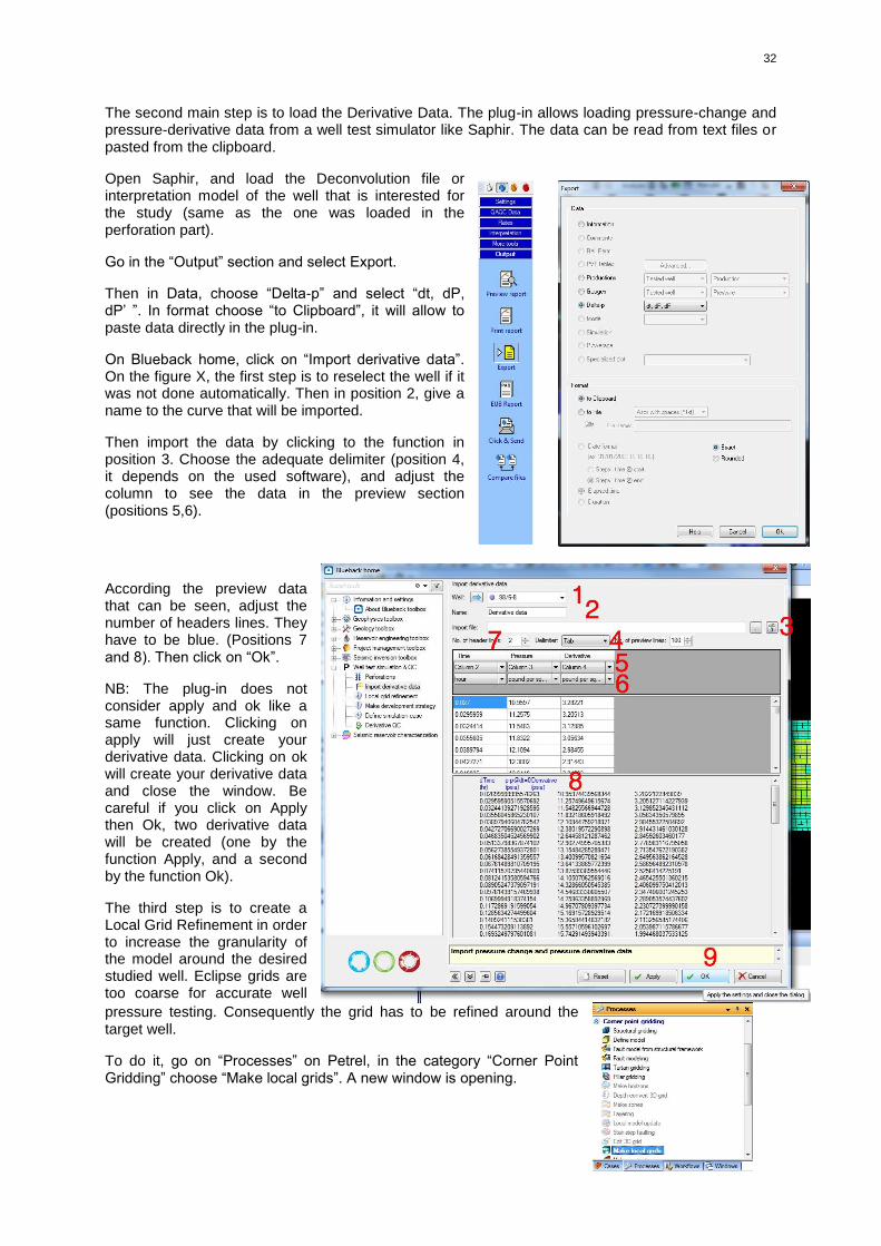
32
The second main step is to load the Derivative Data. The plug-in allows loading pressure-change and pressure-derivative data from a well test simulator like Saphir. The data can be read from text files or pasted from the clipboard.
Open Saphir, and load the Deconvolution file or interpretation model of the well that is interested for the study (same as the one was loaded in the perforation part).
Go in the “Output” section and select Export.
Then in Data, choose “Delta-p” and select “dt, dP, dP’ ”. In format choose “to Clipboard”, it will allow to paste data directly in the plug-in.
On Blueback home, click on “Import derivative data”. On the figure X, the first step is to reselect the well if it was not done automatically. Then in position 2, give a name to the curve that will be imported.
Then import the data by clicking to the function in position 3. Choose the adequate delimiter (position 4, it depends on the used software), and adjust the column to see the data in the preview section (positions 5,6).
According the preview data that can be seen, adjust the number of headers lines. They have to be blue. (Positions 7 and 8). Then click on “Ok”.
NB: The plug-in does not consider apply and ok like a same function. Clicking on apply will just create your derivative data. Clicking on ok will create your derivative data and close the window. Be careful if you click on Apply then Ok, two derivative data will be created (one by the function Apply, and a second by the function Ok).
The third step is to create a Local Grid Refinement in order to increase the granularity of the model around the desired studied well. Eclipse grids are too coarse for accurate well
pressure testing. Consequently the grid has to be refined around the target well.
To do it, go on “Processes” on Petrel, in the category “Corner Point Gridding” choose “Make local grids”. A new window is opening.
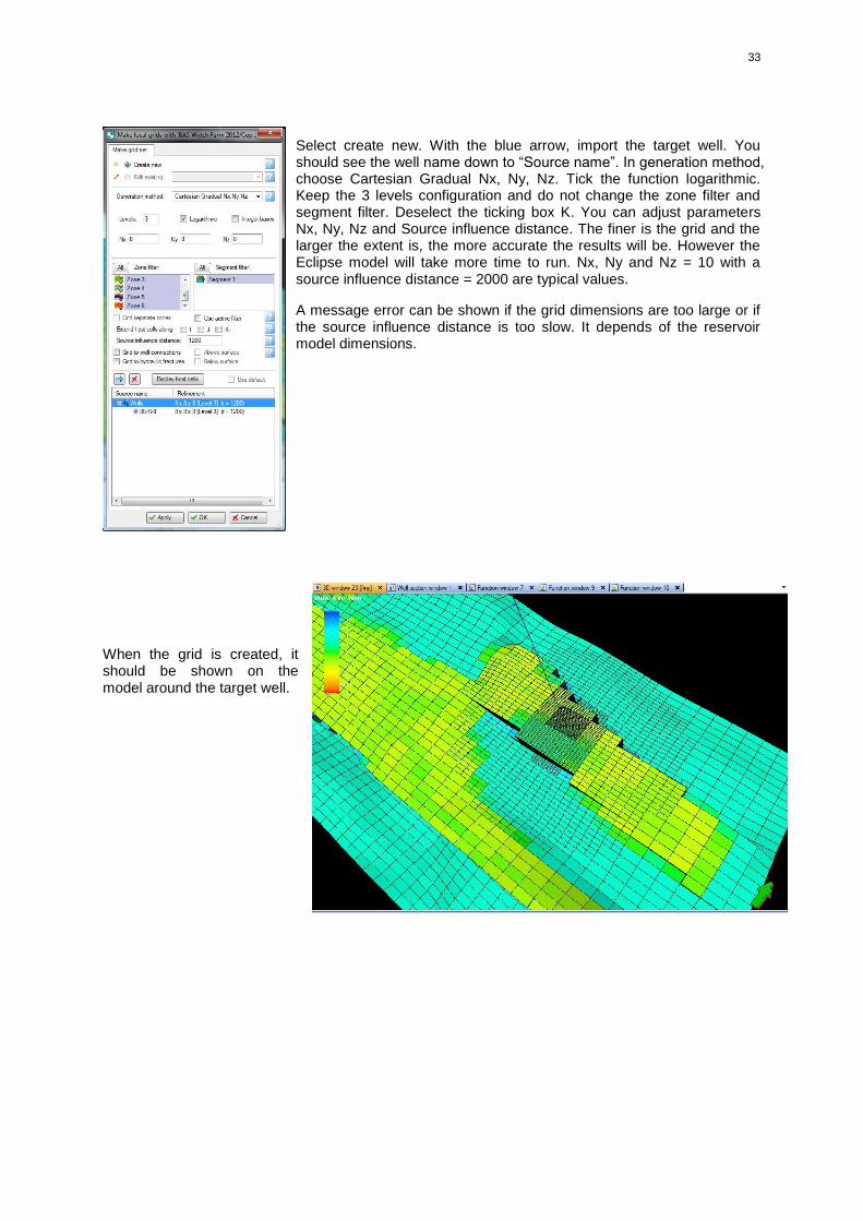
33
Select create new. With the blue arrow, import the target well. You should see the well name down to “Source name”. In generation method, choose Cartesian Gradual Nx, Ny, Nz. Tick the function logarithmic. Keep the 3 levels configuration and do not change the zone filter and segment filter. Deselect the ticking box K. You can adjust parameters Nx, Ny, Nz and Source influence distance. The finer is the grid and the larger the extent is, the more accurate the results will be. However the Eclipse model will take more time to run. Nx, Ny and Nz = 10 with a source influence distance = 2000 are typical values.
A message error can be shown if the grid dimensions are too large or if the source influence distance is too slow. It depends of the reservoir model dimensions.
When the grid is created, it should be shown on the model around the target well.
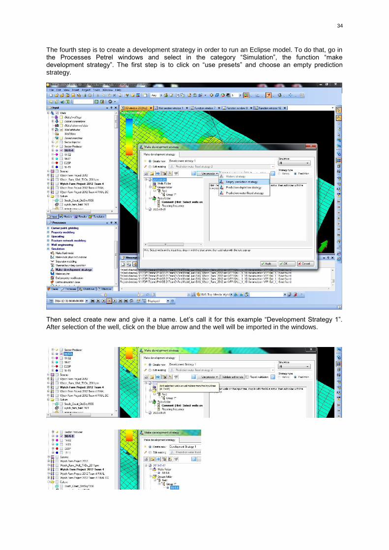
34
The fourth step is to create a development strategy in order to run an Eclipse model. To do that, go in the Processes Petrel windows and select in the category “Simulation”, the function “make development strategy”. The first step is to click on “use presets” and choose an empty prediction strategy.
Then select create new and give it a name. Let’s call it for this example “Development Strategy 1”. After selection of the well, click on the blue arrow and the well will be imported in the windows.
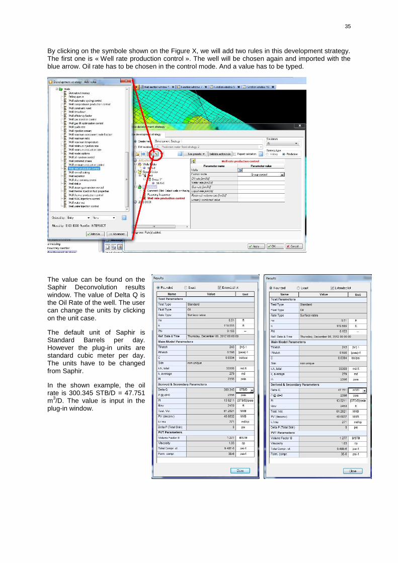
35
By clicking on the symbole shown on the Figure X, we will add two rules in this development strategy. The first one is « Well rate production control ». The well will be chosen again and imported with the blue arrow. Oil rate has to be chosen in the control mode. And a value has to be typed.
The value can be found on the Saphir Deconvolution results window. The value of Delta Q is the Oil Rate of the well. The user can change the units by clicking on the unit case.
The default unit of Saphir is Standard Barrels per day. However the plug-in units are standard cubic meter per day. The units have to be changed from Saphir.
In the shown example, the oil rate is 300.345 STB/D = 47.751 m
3/D. The value is input in the
plug-in window.

36
The value can be shown on the figure X. Then the rule can be validated and a new rule can be added: Derivative Timestep.
Then, in derivation data, select the derivative data that you imported from Saphir at the beginning for the corresponding well and choose it. Adapt the minimum and maximum time step values according to the length of the well test length. And validate the rule.
Before closing the development strategy window, delete the “reporting frequency” rule. It is automatically created when an empty development strategy is run, however the well test analysis does not need to be reported every year, so the rule has to be deleted otherwise it will show wrong results.
Finally close the window by clicking Ok.
The fifth step is to define a simulation case with the development strategy created.
In Processes, Simulation, select “Define simulation case”. A new window is opened. Give a name to the new simulation case; be careful some characters are not accepted by the plug-in.
In simulator select Well Test E100, and be sure that in type, single porosity is chosen and in the grid field, the correct model is selected (in which the local grid is created).
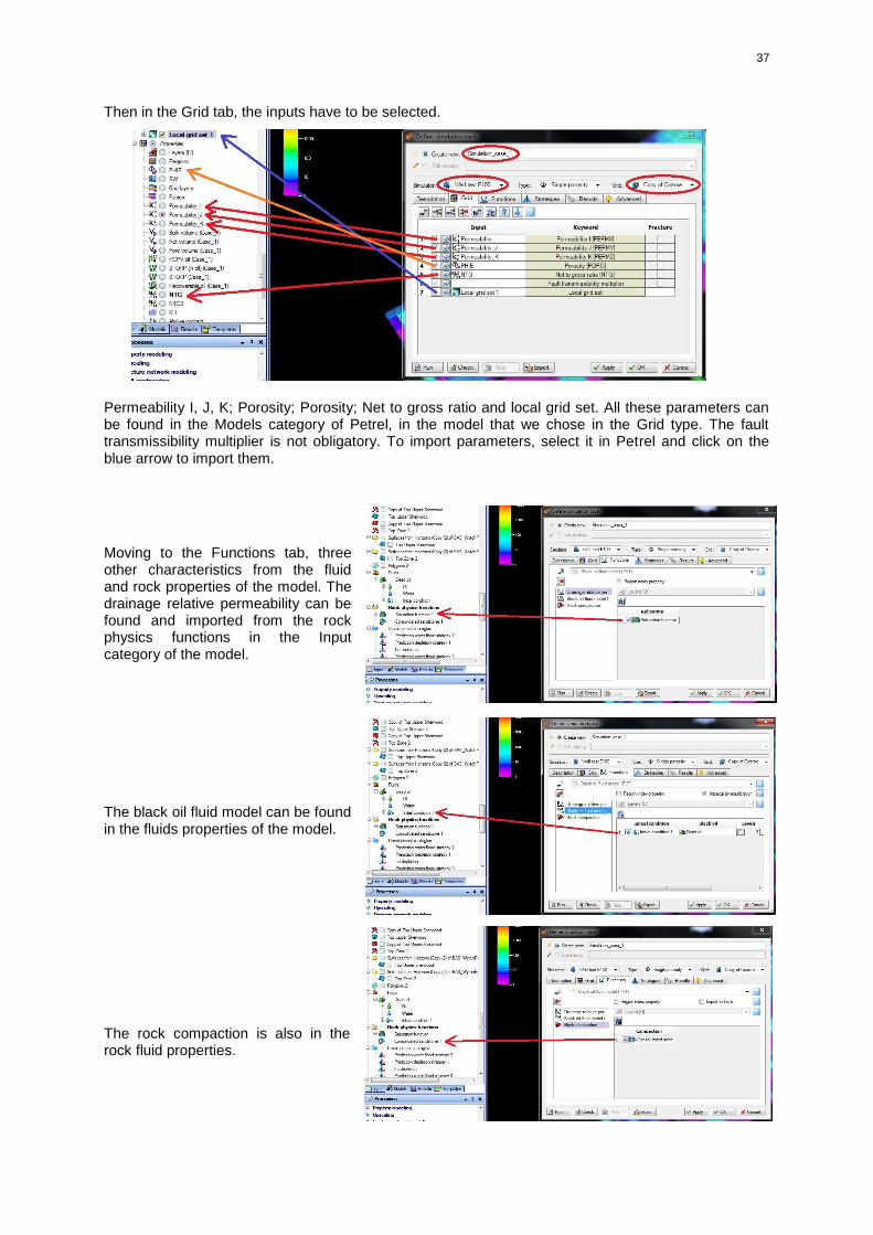
37
Then in the Grid tab, the inputs have to be selected.
Permeability I, J, K; Porosity; Porosity; Net to gross ratio and local grid set. All these parameters can be found in the Models category of Petrel, in the model that we chose in the Grid type. The fault transmissibility multiplier is not obligatory. To import parameters, select it in Petrel and click on the blue arrow to import them.
Moving to the Functions tab, three other characteristics from the fluid and rock properties of the model. The drainage relative permeability can be found and imported from the rock physics functions in the Input category of the model.
The black oil fluid model can be found in the fluids properties of the model.
The rock compaction is also in the rock fluid properties.

38
In the Strategies tab, the development strategy created earlier has to be imported. It can be found in the development strategies file of Petrel in the Models category.
In the results tab, select only wells, oil, rates and pressures in the summary vectors category. In others select limited results only. Then run the simulation case and click on Ok.
A simulation case appears in the cases of Petrel window.
Select it and go back in the blueback plug-in windows in the category Derivative QC.
In Derivative data, select the derivative data imported from Saphir at the beginning of the process.
Then our simulation case should appear in the display, select it and the curves should appear on the graph.
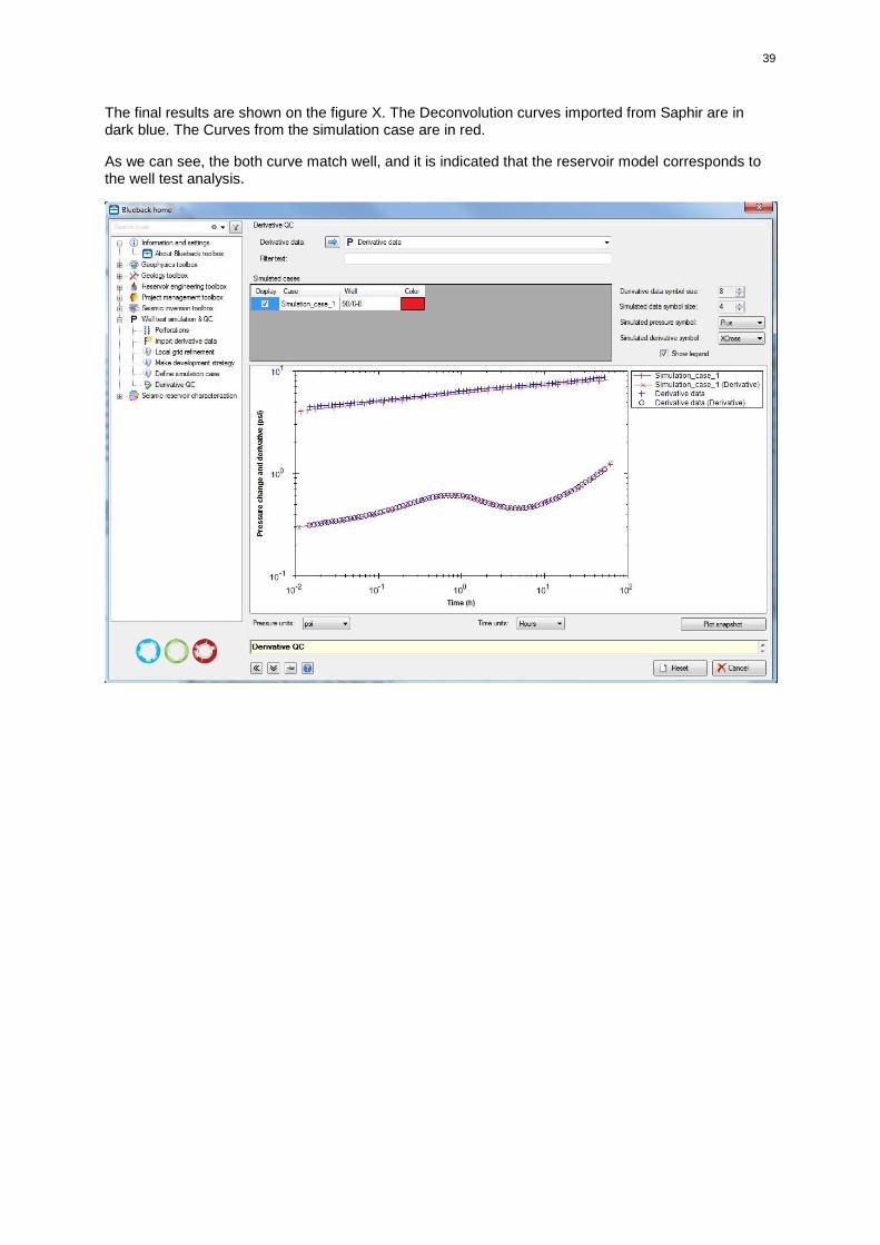
39
The final results are shown on the figure X. The Deconvolution curves imported from Saphir are in dark blue. The Curves from the simulation case are in red.
As we can see, the both curve match well, and it is indicated that the reservoir model corresponds to the well test analysis.
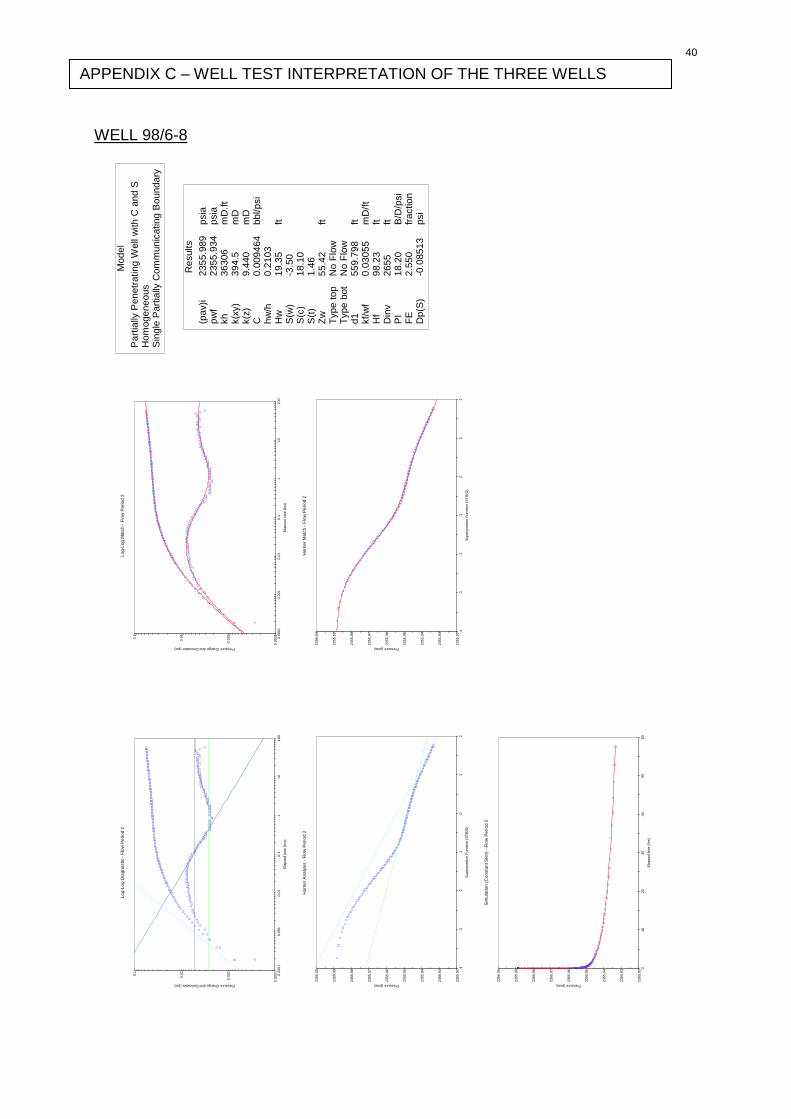
40
0.0
001
0.0
01
0.0
1
0.1
0.0
001
0.0
01
0.0
10.1
110
100
Pressure Change and Derivative (psi)
Ela
psed t
ime (
hrs
)
Lo
g-L
og
Dia
gn
ostic -
Flo
w P
eri
od
2
0.0
001
0.0
01
0.0
1
0.1
0.0
001
0.0
01
0.0
10.1
110
100
Pressure Change and Derivative (psi)
Ela
psed t
ime (
hrs
)
Lo
g-L
og
Ma
tch
- F
low
Pe
rio
d 2
2355.9
2
2355.9
3
2355.9
4
2355.9
5
2355.9
6
2355.9
7
2355.9
8
2355.9
9
2356.0
0 -4-3
-2-1
01
2
Pressure (psia)
Superp
ositio
n F
unction (
ST
B/D
)
Ho
rne
r A
na
lysis
- F
low
Pe
rio
d 2
2355.9
2
2355.9
3
2355.9
4
2355.9
5
2355.9
6
2355.9
7
2355.9
8
2355.9
9
2356.0
0 -4-3
-2-1
01
2
Pressure (psia)S
uperp
ositio
n F
unctio
n (
ST
B/D
)
Ho
rne
r M
atc
h -
Flo
w P
eri
od
2
2355.9
2
2355.9
3
2355.9
4
2355.9
5
2355.9
6
2355.9
7
2355.9
8
2355.9
9
2356.0
0
010
20
30
40
50
60
Pressure (psia)
Ela
psed t
ime (
hrs
)
Sim
ula
tio
n (
Co
nsta
nt
Skin
) -
Flo
w P
eri
od
2
Mo
del
Pa
rtia
lly P
enetr
atin
g W
ell
with
C a
nd
S H
om
ogen
eo
us
Sin
gle
Pa
rtia
lly C
om
mu
nic
atin
g B
ou
ndary
Re
sults
(pav)i
23
55.9
89
psia
pw
f 2
355.9
34
psia
kh
36
306
mD
.ft
k(x
y)
39
4.5
mD
k(z
) 9
.44
0 m
D C
0.0
09
464
bb
l/p
si
hw
/h 0
.21
03
Hw
19
.35
ft S
(w)
-3.5
0 S
(c)
18
.10
S(t
) 1
.46
Zw
55
.42
ft T
ype t
op
No
Flo
w T
ype b
ot
No
Flo
w d
1 5
59.7
98
ft kf/
wf
0.0
30
55
mD
/ft
Hf
98
.23
ft D
inv
26
55
ft P
I 1
8.2
0 B
/D/p
si
FE
2.5
50
fra
ctio
n D
p(S
) -0
.08
513
psi
WELL 98/6-8
APPENDIX C – WELL TEST INTERPRETATION OF THE THREE WELLS

41
WELL D2

42
WELL 98/6-7
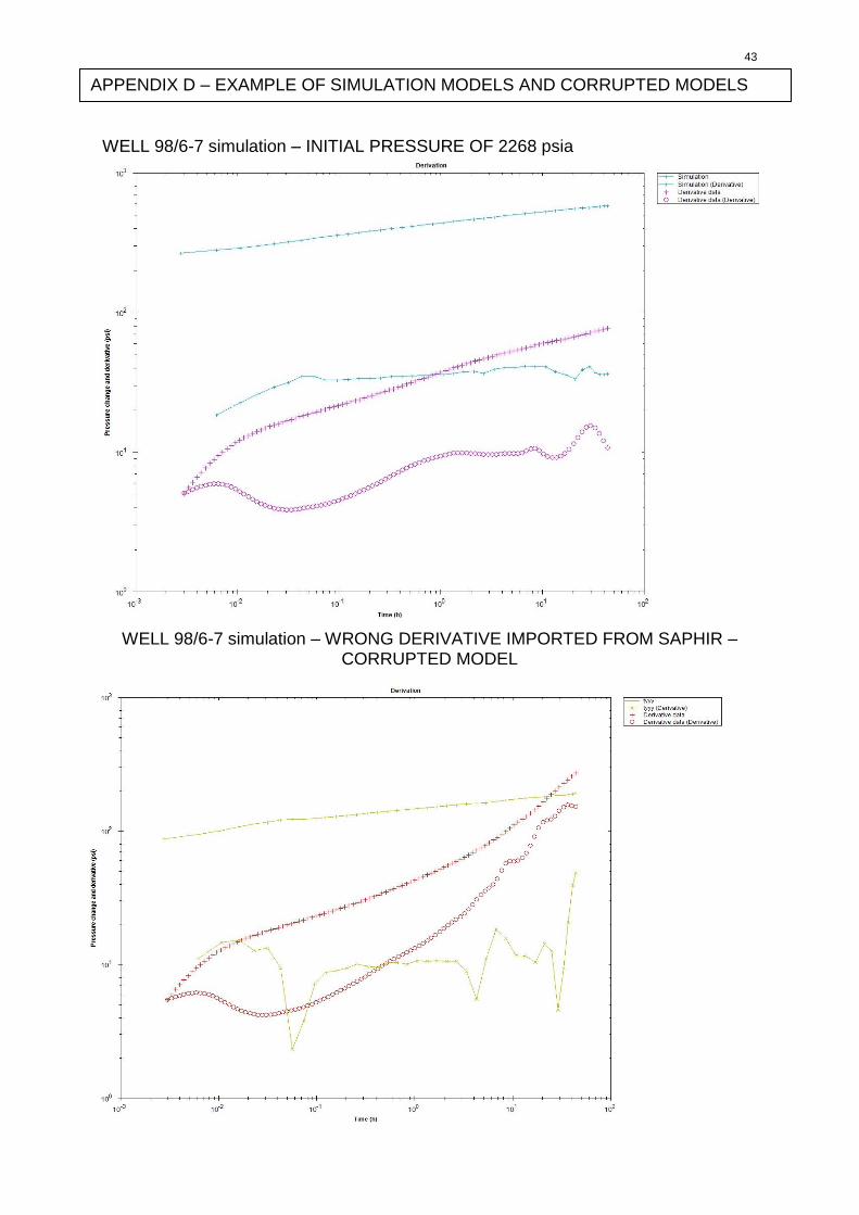
43
WELL 98/6-7 simulation – INITIAL PRESSURE OF 2268 psia
WELL 98/6-7 simulation – WRONG DERIVATIVE IMPORTED FROM SAPHIR – CORRUPTED MODEL
APPENDIX D – EXAMPLE OF SIMULATION MODELS AND CORRUPTED MODELS

44
WELL 98/6-7 simulation – INITIAL PRESSURE OF 2270 psia
WELL 98/6-7 simulation – Wrong derivative imported from Saphir – Initial pressure of 2325 psia

45
WELL 98/6-8 simulation – INITIAL PRESSURE OF 2358 psia
WELL 98/6-8 simulation – INITIAL PRESSURE OF 2359 psia
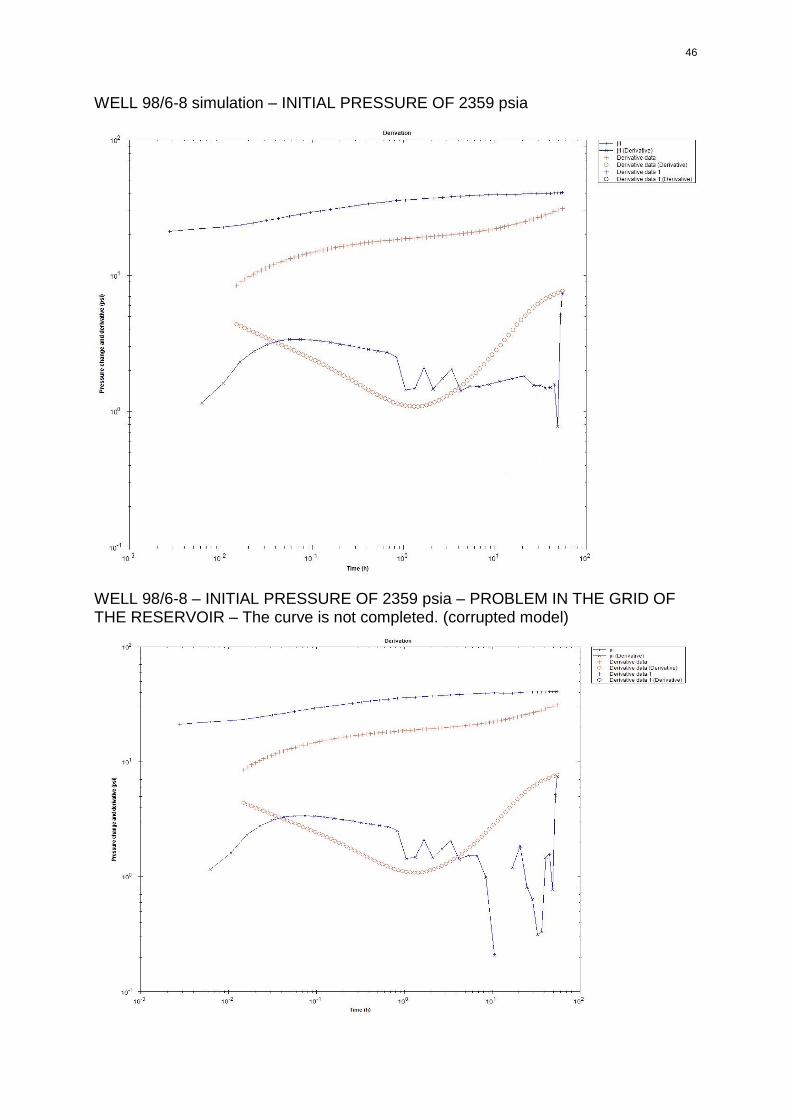
46
WELL 98/6-8 simulation – INITIAL PRESSURE OF 2359 psia
WELL 98/6-8 – INITIAL PRESSURE OF 2359 psia – PROBLEM IN THE GRID OF THE RESERVOIR – The curve is not completed. (corrupted model)

47
WELL 98/6-8 – INITIAL PRESSURE OF 2359 psia
WELL D2 – INITIAL PRESSURE OF 2403 psia

48
APPENDIX E – IMPACT OF THE MULTIPLICATION OF PERMEABILITY I ON THE WELL 98/6-8

49
APPENDIX F – IMPACT OF THE MULTIPLICATION OF PERMEABILITY J ON THE WELL 98/6-8

50
APPENDIX G – UNCERTAINTY ANALYSIS WITH THE SOFTWARE R.
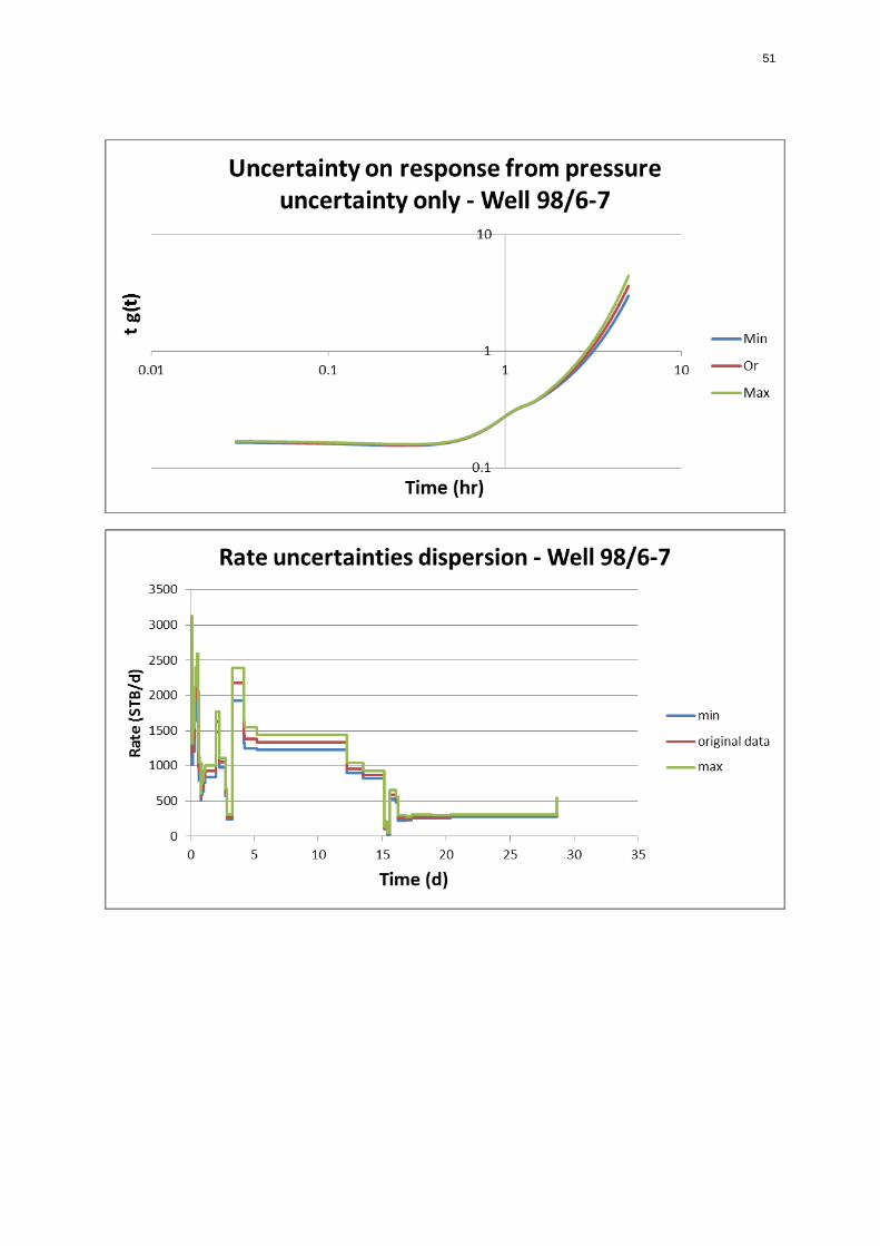
51
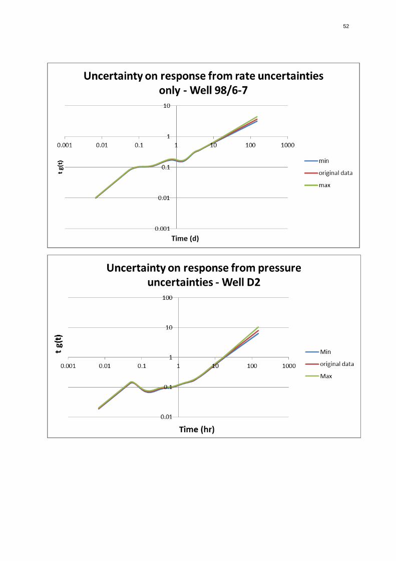
52

53
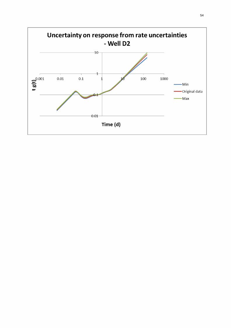
54

55
WELL D2
APPENDIX H – ASSOCIATED HISTORY MATCH FOR THREE WELLS.
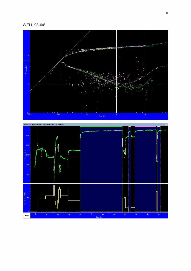
56
WELL 98-6/8
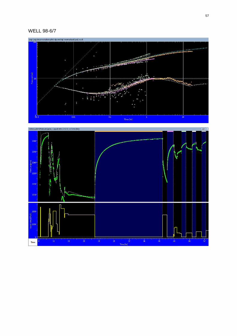
57
WELL 98-6/7