impacts of land management options in the upper tana ... · green water is moisture held in the...
TRANSCRIPT
ISRIC – World Soil Information has a mandate to serve the international community as custodian of global soil information and to increase awareness and understanding of soils in major global issues.
More information: www.isric.org
ISRIC – World soil Information has a strategic association with Wageningen UR (University & Research centre)
Green Water Credits Report 10
J.E. Hunink, W.W. Immerzeel, P. Droogers, J.H. Kauffman and G.W.J. van Lynden
Impacts of Land Management Options in the Upper Tana, Kenya Using the Soil and Water Assessment Tool - SWAT

Green Water Credits
Impacts of Land Management Options in the Upper Tana, Kenya Using the Soil and Water Assessment Tool - SWAT
Authors J.E. Hunink W.W. Immerzeel P. Droogers J.H. Kauffman G.W.J. van Lynden Series Editors W.R.S. Critchley E.M. Mollee
Green Water Credits Report 10 / Report FutureWater 84 Wageningen, 2011
Ministry of Agriculture
Water Resources Management Authority
Ministry of Water and Irrigation

© 2011, ISRIC Wageningen, Netherlands All rights reserved. Reproduction and dissemination for educational or non-commercial purposes are permitted without any prior written permission provided the source is fully acknowledged. Reproduction of materials for resale or other commercial purposes is prohibited without prior written permission from ISRIC. Applications for such permission should be addressed to: Director, ISRIC – World Soil Information PO B0X 353 6700 AJ Wageningen The Netherlands E-mail: [email protected] The designations employed and the presentation of materials do not imply the expression of any opinion whatsoever on the part of ISRIC concerning the legal status of any country, territory, city or area or of is authorities, or concerning the delimitation of its frontiers or boundaries. Despite the fact that this publication is created with utmost care, the authors(s) and/or publisher(s) and/or ISRIC cannot be held liable for any damage caused by the use of this publication or any content therein in whatever form, whether or not caused by possible errors or faults nor for any consequences thereof. Additional information on ISRIC – World Soil Information can be accessed through http://www.isric.org Citation J.E. Hunink, W.W. Immerzeel, P. Droogers, S. Kauffman and G. van Lynden. 2011. Impacts of Land Management Options in the Upper Tana, Kenya; Using the Soil and Water Assessment Tool – SWAT. Green Water Credits Report 10, ISRIC – World Soil Information, Wageningen.
Submitted by
FutureWater Costerweg 1G 6702 AA Wageningen, The Netherlands Phone: +31 (0)317 460050 E-mail: [email protected] www.futurewater.nl
Green Water Credits Report 10

Green Water Credits Report 10 3
Foreword
ISRIC – World Soil Information has the mandate to create and increase the awareness and understanding of the role of soils in major global issues. As an international institution, ISRIC informs a wide audience about the multiple roles of soils in our daily lives; this requires scientific analysis of sound soil information. The source of all fresh water is rainfall received and delivered by the soil. Soil properties and soil management, in combination with vegetation type, determine how rain will be divided into surface runoff, infiltration, storage in the soil and deep percolation to the groundwater. Improper soil management can result in high losses of rainwater by surface runoff or evaporation and may in turn lead to water scarcity, land degradation, and food insecurity. Nonetheless, markets pay farmers for their crops and livestock but not for their water management. The latter would entail the development of a reward for providing a good and a service. The Green Water Credits (GWC) programme, coordinated by ISRIC – World Soil information and supported by the International Fund for Agricultural Development (IFAD) and the Swiss Agency for Development and Cooperation (SDC), addresses this opportunity by bridging the incentive gap. Much work has been carried out in the Upper Tana catchment, Kenya, where target areas for GWC intervention have been assessed using a range of biophysical databases, analysed using crop growth and hydrological modelling. The Proof-of-Concept phase of Green Water Credits showed that the Soil and Water Assessment Tool (SWAT) was appropriate to study, and quantify, the up- and downstream interactions in the Upper Tana catchment, as well as the influence of land use and management on water resources and sediment transport in the catchment. The model quantifies the benefits of various green water management practices. It shows how much erosion and reservoir sediment input can be reduced, and how green water/ blue water partitioning can be optimised through different management options. Results of this biophysical suitability assessment will provide input into the forthcoming studies on socio-economic and institutional issues in the areas. This will lead to the final selection of the pilot operation areas. Dr ir Prem Bindraban Director, ISRIC – World Soil Information

4 Green Water Credits Report 10
Key Points
– The Proof-of-Concept phase of Green Water Credits showed that the Soil and Water Assessment Tool (SWAT) was appropriate to study, and quantify, the up- and downstream interactions in the Upper Tana catchment, as well as the influence of land use and management on water resources and sediment transport in the catchment.
– The model quantifies the benefits of various green water management practices. It shows how much
erosion and reservoir sediment input can be reduced, and how green water/ blue water partitioning can be optimised through different management options.
– It is clear that the soil and aquifer reservoirs have the potential to improve the management of water
resources in the basin as they assure a more continuous and reliable flow regime. Green water management options aim at maximising the potential of these natural reservoirs.
– The analysis revealed that basin-wide implementation of tied ridges would lead to a reduction of sediment
input into the Masinga reservoir of about a million tonnes per year. Mulching would reduce unproductive soil evaporation by more than 100 million cubic meters per year.
– Implementation of one of the green water management practices will approximately halve the rate of
erosion in the higher, steeper areas. Green water practices are more effective in these areas because they receive more rainfall than the lower parts of the basin.
– The enhancement of groundwater recharge through the different practices would improve the usage of the
natural storage capacity in the basin by about 20%. These benefits were quantified crop-specifically as well as site-specifically.
– This assessment shows an unambiguous benefit by optimising the use of the aquifer as a natural water
storage facility. The reduction of runoff and the parallel enhancement of percolation and groundwater recharge reduce unproductive outflow from the reservoirs during intense rainfall periods, as more water is retained upstream within the soil and aquifer. This stimulates a more continuous and reliable water supply during ensuing dry periods.
– The distributed approach made it possible to assess the spatial distribution of the extent to which each
practice contributes to the different GWC objectives. The most effective practices were determined for each response unit (unique in topography, soil and land use) and the maximum attainable change was gauged.
– An addendum was judged necessary as new information became available on land use and soils within the
Upper Tana catchment. However the key indicators used to quantify the impact of the green water management options showed very similar results. This implies that the same conclusions can be drawn regarding the potential of the management options to meet the Green Water Credits objectives.
– Results of this biophysical suitability assessment will provide input into the forthcoming studies on socio-
economic and institutional issues in the areas. This will lead to the final selection of the pilot operation areas.

Green Water Credits Report 10 5
Contents
Foreword 3
Key Points 4
Contents 5
Acronyms and Abbreviations 7
1 Introduction 11
2 Baseline information 13
3 Baseline model analysis 49
4 Options for Green Water Credits 69
References 91
Addendum I 93
Summary 95
5 Model revision 97
6 Scenario analysis 103
7 Conclusions 113
Addendum II 115
8 Introduction 117
9 Green water management measures 119
10 Results 127

6 Green Water Credits Report 10

Green Water Credits Report 10 7
Acronyms and Abbreviations
AEZ Agro-Ecological Zone AMSU Advanced Microwave Sounding Unit ASAL Arid and Semi-Arid Lands BSI Biophysical Suitability Index CPC Climate Prediction Center CRU Climate Research Unit of the University of East Anglia DEM Digital Elevation Model DTR Diurnal Temperature Range EEA European Environment Agency EROS Earth Resources Observation and Science ESA European Space Agency ESCO Soil Evaporation Compensation factor FAO Food and Agriculture Organisation FEWS NET Famine Early Warning System Network GOFC-GOLD Global Observation for Forest and Land Cover Dynamics GRDD Global River Discharge Database GSOD Global Summary of the Day GTS Global Telecommunications System GWC Green Water Credits HRU Hydrological Response Unit IGBP International Geosphere-Biosphere Programme ISRIC ISRIC – World Soil Information JPL Jet Propulsion Laboratory JRC Joint Research Centre of the European Commission KSS Kenya Soil Survey LCCS Land Cover Classification System MUSLE Modified Universal Soil Loss Equation MWD Ministry of Water Development NASA National Aeronautics and Space Administration NCDC National Climatic Data Center NRCS Natural Resources Conservation Service PoC Proof-of-Concept PTF Pedotransfer Function RMS Root Mean Square SOTER Soil and Terrain database SOTWIS Harmonised continental SOTER-derived database SRTM Shuttle Radar Data Topography Mission SSM/I Special Sensor Microwave/Imager SVM Support Vector Machine SWAT Soil and Water Assessment Tool

8 Green Water Credits Report 10
UNEP United Nations Environment Programme UoN University of Nairobi USAID United States Agency for International Development USLE Universal Soil Loss Equation WRMA Water Resources Management Authority WOCAT World Overview of Conservation Approaches and Technologies

Green Water Credits Report 10 9

10 Green Water Credits Report 10
Green Water Credits: the concepts
Green water, Blue water, and the GWC mechanism
Green water is moisture held in the soil. Green water flow refers to its return as vapour to the atmosphere through transpiration by plants or from the soil surface through evaporation. Green water normally represents the largest component of precipitation, and can only be used in situ. It is managed by farmers, foresters, and pasture or rangeland users. Blue water includes surface runoff, groundwater, stream flow and ponded water that is used elsewhere - for domestic and stock supplies, irrigation, industrial and urban consumption. It also supports aquatic and wetland ecosystems. Blue water flow and resources, in quantity and quality, are closely determined by the management practices of upstream land users.
Green water management comprises effective soil and water conservation practices put in place by land users. These practices address sustainable water resource utilisation in a catchment, or a river basin. Green water management increases productive transpiration, reduces soil surface evaporation, controls runoff, encourages groundwater recharge and decreases flooding. It links water that falls on rainfed land, and is used there, to the water resources of rivers, lakes and groundwater: green water management aims to optimise the partitioning between green and blue water to generate benefits both for upstream land users and downstream consumers. Green Water Credits (GWC) is a financial mechanism that supports upstream farmers to invest in improved green water management practices. To achieve this, a GWC fund needs to be created by downstream private and public water-use beneficiaries. Initially, public funds may be required to bridge the gap between investments upstream and the realisation of the benefits downstream. The concept of green water and blue water was originally proposed by Malin Falkenmark as a tool to help in the understanding of different water flows and resources - and the partitioning between the two (see Falkenmark M 1995 Land-water linkages. FAO Land and Water Bulletin 15-16, FAO, Rome).
Green Water Credits Report 10 11
1 Introduction
In Kenya, Proof-of-Concept studies during Phase I showed that the implementation of Green Water Credits can significantly reduce the problems related to the growing demands for hydro-power generation, municipal water utilities, and irrigation. Different green water management options were analysed, and showed that considerable improvements could be obtained in terms of water security for both upstream and downstream stakeholders. Based on the Proof-of-Concept phase it was concluded that, regarding the biophysical analysis, the following refinements are required during Phase II: – A smaller area of focus: namely from Upper and Middle Tana to Upper Tana only. – A higher spatial detail so that smaller areas could be assessed. – Focus on more recent years. – Improved accuracy and higher spatial (from 25 km to 1 km) and temporal (from month to day) resolution of
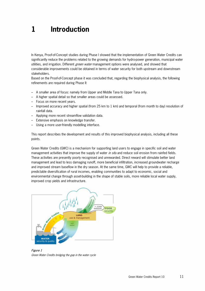
rainfall data. – Applying more recent streamflow validation data. – Extensive emphasis on knowledge transfer. – Using a more user-friendly modelling interface. This report describes the development and results of this improved biophysical analysis, including all these points. Green Water Credits (GWC) is a mechanism for supporting land users to engage in specific soil and water management activities that improve the supply of water in situ and reduce soil erosion from rainfed fields. These activities are presently poorly recognised and unrewarded. Direct reward will stimulate better land management and lead to less damaging runoff, more beneficial infiltration, increased groundwater recharge and improved stream baseflow in the dry season. At the same time, GWC will help to provide a reliable, predictable diversification of rural incomes, enabling communities to adapt to economic, social and environmental change through asset-building in the shape of stable soils, more reliable local water supply, improved crop yields and infrastructure.
Figure 1
Green Water Credits bridging the gap in the water cycle

12 Green Water Credits Report 10

Green Water Credits Report 10 13
2 Baseline information
For the pilot operational design of the Green Water Credits concept it is crucial to fully understand and quantify the up- and downstream interactions of water flows and sediment transport. Consequently, accurate data on the variables of the current situation are required, and need to be analysed with an appropriate tool. During the Proof-of-Concept phase different tools were assessed, and the Soil and Water Assessment Tool (SWAT) was demonstrated to be the most useful tool for this biophysical analysis, given the importance of studying the influence of land use on water dynamics in the basin. This chapter reviews the available datasets necessary for the building of a distributed hydrological model applicable to the Upper Tana catchment, using the Soil and Water Assessment Tool. Different datasets are compared and evaluated in order to make an appropriate dataset selection, and obtain maximum accuracy, in the quantification of the interactions relevant for the Green Water Credits mechanism. 2.1 Basin delineation
2.1.1 Data source
Digital Elevation data were obtained from the Shuttle Radar Data Topography Mission (SRTM) of NASA’s Space Shuttle Endeavour flight on 11-22 February 2000. SRTM data were processed from raw radar echoes into digital elevation models at the Jet Propulsion Laboratory (JPL) in California.
Figure 2
The SRTM Digital Elevation Model at 250 m resolution

14 Green Water Credits Report 10
SRTM data at 3 arc-second (90 meters) is currently available for global coverage between 60 degrees North and 56 degrees South latitude. The product consists of seamless raster data and is available in geographic coordinates (latitude/longitude) and is horizontally and vertically referenced to the EGM96 Geoid1. The SRTM-DEM data were obtained using the USGS Seamless Data Distribution System2. 2.1.2 Methodology
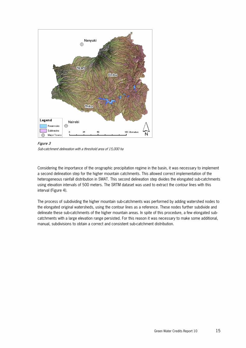
The original SRTM-DEM data are available at a resolution of 90 m. However, the basin size and the numerical limitations of SWAT required this dataset to be resampled to a spatial resolution of 250 m (Figure 2). The basin outlet was defined as the location of the proposed Low Grand Falls dam. Consequently, all the tributaries of the Aberdares and Mount Kenya belonging to the basin are included in the analysis. The DEM forms the base to delineate the catchment boundary, stream network and create sub-basins. This is performed by the pre-processing module of SWAT and requires a “threshold area”. This refers to a critical source defining the minimum drainage area required to form the origin of a stream. The determination of an appropriate threshold area has to be in accordance with the desired level of detail. An appropriate threshold area of 2000 ha was found to provide a good balance between the level of detail and the computational constraints in the lower part of the basin. However, applying this threshold area resulted in very elongated sub-catchments in the higher regions of the Aberdares and Mount Kenya (Figure 3). This implies a large difference between the minimum and maximum elevations within the sub-catchments; reaching around 3000 meters within one sub-catchment.
1 NASA 1998. The NASA GSFC and NIMA (National Imagery and Mapping Agency) Joint Geopotential Model EGM96:
http://cddis.nasa.gov/926/egm96/egm96.html 2 USGS 2004. Earth Resources Observation and Science (EROS) Centre: http://seamless.usgs.gov/
Green Water Credits Report 10 15
Figure 3
Sub-catchment delineation with a threshold area of 15,000 ha
Considering the importance of the orographic precipitation regime in the basin, it was necessary to implement a second delineation step for the higher mountain catchments. This allowed correct implementation of the heterogeneous rainfall distribution in SWAT. This second delineation step divides the elongated sub-catchments using elevation intervals of 500 meters. The SRTM dataset was used to extract the contour lines with this interval (Figure 4). The process of subdividing the higher mountain sub-catchments was performed by adding watershed nodes to the elongated original watersheds, using the contour lines as a reference. These nodes further subdivide and delineate these sub-catchments of the higher mountain areas. In spite of this procedure, a few elongated sub-catchments with a large elevation range persisted. For this reason it was necessary to make some additional, manual, subdivisions to obtain a correct and consistent sub-catchment distribution.

16 Green Water Credits Report 10
Figure 4
Contour lines (500 m) used for the subdivision of the upstream sub-catchments
2.1.3 Results
With the proposed modified delineation methodology, the stream network (Figure 5) and sub-catchments were defined. This resulted in a sub-catchment distribution with a slightly denser distribution in the higher mountain areas (Figure 6) which would allow a correct simulation of the orographic precipitation regime. The result of the analysis showed that the total basin area is 17,420 km2 within which a total of 564 sub-catchments were delineated.

Green Water Credits Report 10 17
Figure 5
The derived stream network
The adjusted frequency distribution of the elevation range now shows that most of the sub-catchments have an elevation range of less than 500 meters (Figure 7), as this was the interval chosen to make the subdivisions using contour lines. Within this elevation interval it is reasonable to assume that there are no significant changes in the precipitation regime. Most of the sub-catchments with a large elevation difference were subdivided by this method, although a few sub-catchments still encompass an elevation difference of around 1000 meters. These sub-catchments, however, correspond to those lower-lying that contain irregularities in terrain morphology; however, it can be assumed that these are too minor to alter the precipitation.

18 Green Water Credits Report 10
Figure 6
The sub-catchments using the modified delineation methodology
Figure 7
Frequency distribution of the difference in elevation within each sub-catchment, with and without refinement using contour lines
2.2 Climate
2.2.1 Climatic conditions
The Upper Tana catchment experiences two wet, and two dry seasons as a result of the monsoon. From mid-March to June the main rainy season, known as the long rains, brings approximately half of the annual rainfall

Green Water Credits Report 10 19
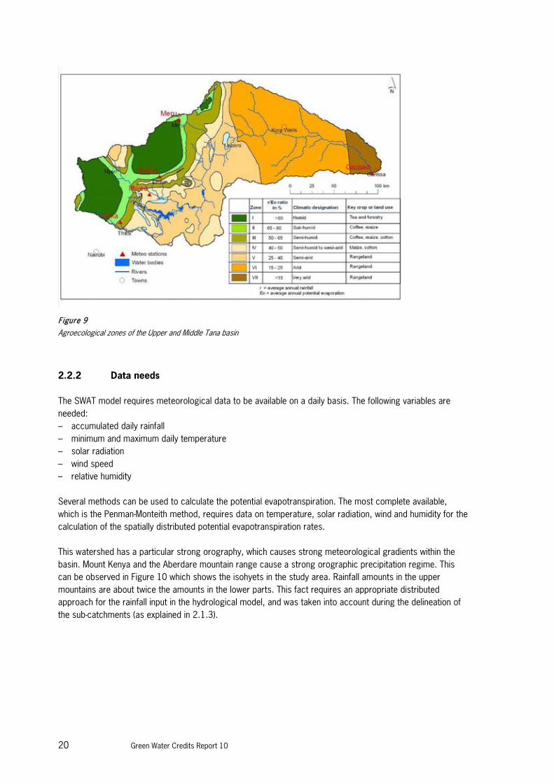
to the basin. This is followed by the wetter of the two dry seasons which lasts until September. October to December bring the so-called short rains when the mountain receives approximately a third of its annual rainfall total. Finally, the period between December and mid-March is the driest of the annual precipitation regime. Figure 8 shows the main agroclimatic zones, based on the balance between precipitation and evapotranspiration (Sombroek et al. 1982). The Upper and Middle Tana basin (outlet at Garissa) encompasses seven main climatic zones, ranging from humid to very arid. Comparing this distribution with the contour lines of Figure 4 it is clear that there is a close correlation between elevation and climatic zones; in other words, annual rainfall increases with elevation. Figure 9 presents the agroecological zones according to the Farm Management Handbook of Kenya (Jaetzold and Schmidt 1983). This map shows more detail than that in Figure 8, although the number and the boundaries of the main zones are very similar. This map characterises the Agro-Ecological Zone (AEZ) according to the main land use, for example humid tea zone, arid rangeland zone etc.
Figure 8
Agroclimatic zones of the Upper and Middle Tana catchment
20 Green Water Credits Report 10
Figure 9
Agroecological zones of the Upper and Middle Tana basin
2.2.2 Data needs
The SWAT model requires meteorological data to be available on a daily basis. The following variables are needed: – accumulated daily rainfall – minimum and maximum daily temperature – solar radiation – wind speed – relative humidity Several methods can be used to calculate the potential evapotranspiration. The most complete available, which is the Penman-Monteith method, requires data on temperature, solar radiation, wind and humidity for the calculation of the spatially distributed potential evapotranspiration rates. This watershed has a particular strong orography, which causes strong meteorological gradients within the basin. Mount Kenya and the Aberdare mountain range cause a strong orographic precipitation regime. This can be observed in Figure 10 which shows the isohyets in the study area. Rainfall amounts in the upper mountains are about twice the amounts in the lower parts. This fact requires an appropriate distributed approach for the rainfall input in the hydrological model, and was taken into account during the delineation of the sub-catchments (as explained in 2.1.3).

Green Water Credits Report 10 21
Figure 10
Isohyetal map of the rainfall distribution in the Upper Tana catchment (Source: MWD 1992)
2.2.3 Data sources
2.2.3.1 Documents
An extensive inventory of historical data can be found in the Study on the National Water Master Plan (MWD 1992). The accompanying book contains statistics and metadata on the meteorological and discharge information available until (approximately) 1985. Some measurements are also included on the suspended loads analysed from samples taken around 1980. The information on meteorological data covers monthly statistics averaged over the full data period available. In some cases the time span of the dataset is very short; around five years. Furthermore, the discharge data given in this report are monthly averages over the whole data period. 2.2.3.2 Data obtained from local databases
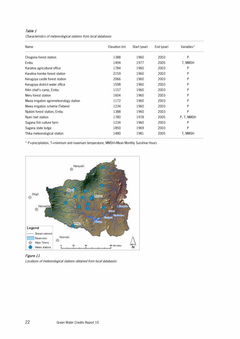
For the Proof-of-Concept phase of Green Water Credits, data from local databases were obtained from various meteorological stations in the basin. All the data have a monthly time basis. The following table gives a summary of their characteristics, and Figure 11 represents their spatial distribution in the basin:
22 Green Water Credits Report 10
Table 1
Characteristics of meteorological stations from local databases
Name Elevation (m) Start (year) End (year) Variables*
Chogoria forest station 1388 1960 2003 P
Embu 1494 1977 2005 T, MMSH
Karatina agricultural office 1784 1960 2003 P
Karatina hombe forest station 2159 1960 2003 P
Kerugoya castle forest station 2066 1960 2003 P
Kerugoya district water office 1598 1960 2003 P
Kitiri chief's camp, Embu 1157 1960 2003 P
Meru forest station 1604 1960 2003 P
Mwea irrigation agrometeorology station 1172 1960 2003 P
Mwea irrigation scheme (Tebere) 1234 1960 2003 P
Njukiini forest station, Embu 1388 1960 2003 P
Nyeri met station 1780 1978 2005 P, T, MMSH
Sagana fish culture farm 1234 1960 2003 P
Sagana state lodge 1850 1969 2003 P
Thika meteorological station 1480 1981 2005 T, MMSH
* P=precipitation, T=minimum and maximum temperature, MMSH=Mean Monthly Sunshine Hours
Figure 11
Locations of meteorological stations obtained from local databases

Green Water Credits Report 10 23
2.2.3.3 The Weather Underground database
The Weather Underground archive has an extensive amount of data available for downloading from stations all over the world3.Within the study basin only one station was found - Meru - shown in the north-eastern part of Figure 12. However, the stations in Nairobi (south) and Nakuru (north-west) are relatively close to the basin.
Figure 12
Availability of stations in the Weather Underground archive
2.2.3.4 The GSOD database
Meteorological data from weather stations all over the world can be found at the public domain Global Summary of the Day (GSOD) database archived by the National Climatic Data Center (NCDC). This database offers a substantial number of stations with long-term daily time series. The GSOD database submits all series (regardless of origin) to extensive automated quality control. Therefore, it can be considered a uniform and validated database in which errors have been eliminated.
3 www.wunderground.com

24 Green Water Credits Report 10
Figure 13
Locations of active local meteorological weather stations: GSOD database
In the study basin there are three currently active stations from which data can be downloaded (Figure 13). A shortcoming is that the location of these three weather stations is more or less within the same climatic zone. Table 2 shows the elevation of the stations, ranging from 1493 to 1759 m.a.s.l. No active or inactive weather stations were found in the lower semi-arid areas or in the humid high mountain areas.
Table 2
Characteristics of active local meteorological stations: GSOD database
Station name Latitude Longitude Elevation Data Period
MERU 0.08 37.65 1554 1914 - 2009 NYERI -0.50 36.97 1759 1920 - 2009 EMBU -0.50 37.45 1493 1908 - 2009
2.2.3.5 The CRU dataset
The Climate Research Unit (CRU) of the University of East Anglia gathered the CRU TS 2.0 dataset that comprises 1200 monthly grids of observed climate, for the period 1901-2000, and covers the global land surface at 0.5 degree resolution. There are five climatic variables available: cloud cover, DTR, precipitation, temperature and vapour pressure. The observed grids are based exclusively on meteorological measurements from individual stations, and no remote sensing information was included. Coverage of the stations used for the interpolation of the grids was found to be sparse on the African continent. Therefore, it was assumed that if there is no adjacent station information available, the best estimate of a certain point in the grid is the long-term average value. The interpolation method used to create the continuous grids is termed “relaxation to the climatology”.

Green Water Credits Report 10 25
The fact that the interpolated grids are based only on scarce station information from the African continent makes this dataset less reliable for hydrological modelling of an area with large climatic differences such as the Tana basin. 2.2.3.6 The FEWS network
One-day estimates of precipitation for Africa are prepared operationally at the Climate Prediction Center (CPC) for the United States Agency for International Development (USAID) as a part of the Famine Early Warning System Network (FEWS NET). The algorithm for the rainfall estimates uses Meteosat 7 geostationary satellite infrared data that are acquired in 30-minute intervals, and areas depicting cloud-top temperatures of less than 235K are used to estimate convective rainfall. Two other satellite rainfall estimation instruments are incorporated into the algorithm, these being the Special Sensor Microwave/Imager (SSM/I) on board Defense Meteorological Satellite Program (DMSP) satellites, and the Advanced Microwave Sounding Unit (AMSU). All satellite data are first combined using a maximum likelihood estimation method, and then GTS station data are used to remove bias. Warm cloud precipitation estimates are not included in the algorithm. CPC/FEWS Estimates are available from October 2000 with a spatial resolution of 0.1 degree. Figure 14 shows an example of the rainfall estimate covering whole Africa.
Figure 14
Rainfall estimates obtained from the FEWS network (24/11/2000)
2.2.4 Dataset evaluation
2.2.4.1 Data Availability
Table 3 summarises the characteristics of the different available data sources. The temporal and spatial resolution of the datasets are of particular importance for consistent model implementation.

26 Green Water Credits Report 10
Table 3
Characteristics of different meteorological data sources
Name Type Format Temporal
resolution
Nr. stations* /
Spatial resolution
Availability Variables**
Presently available
Local Data
Observed Station Monthly 8 1960 - 2003 P, Tmax, Tmin, MSHM
Weather Underground
Archive
Observed Station Daily 1 - present P, Tmax, Tmin, DEWPT,
WNDAV,
GSOD database Observed Station Daily 3 - present P, Tmax, Tmin, DEWPT,
WNDAV,
CRU interpolation
grids
Interpolated with
station data
Grid Monthly 0.5° - 2000 P, CC, DTR, T, VP
FEWS grid estimates Estimated with RS Grid Daily 0.1° 2000 -
present
P
* The number of available stations present within the study basin ** P=precipitation, Tmax=maximum temperature, Tmin= minimum temperature, T= temperature, MSHM=mean sunshine hours month, DEWPT=Dew point, WNDAV=Average wind speed, CC=Cloud cover, DTR=Diurnal temperature range, VP=Vapour pressure
As can be seen from Table 3, only the FEWS precipitation estimates and the GSOD database provide daily data. For this reason, the following dataset evaluation was exclusively based on these. 2.2.4.2 Missing values
An important issue to deal with is the number of missing daily values and the methodology used to estimate them. A few years in the dataset from the GSOD database contain a considerable number of missing daily values, while the estimates of the FEWS network do have more constant coverage. Besides, most of the missing values found in the FEWS dataset are during the usually dry month of July in 2006, which means that these missing values are of minor importance. Table 4 shows the missing daily values found in both datasets.
Table 4
Missing daily values in the estimated (FEWS) and observed datasets
Year FEWS grids Embu station Meru station Nyeri station
2001 56 7 47
2002 48 10 40
2003 1 85 4 87
2004 1 208 26 132
2005 140 40 80
2006 15 60 22 30
2007 1 49 25 16
2008 72 59 23
2009 24 4 10

Green Water Credits Report 10 27
2.2.4.3 Evaluation of daily data
To be able to compare both datasets, time series were extracted from the daily FEWS grids for the location of the three weather stations. Consequently, the time series of the observed values from the GSOD database were compared with the estimates of the FEWS network. It was observed that there is a one-day time lag between the datasets, which presumably means that the timestamp of one (or both) datasets contains a small error. This was corrected for the comparative analysis. Figure 15 gives the daily values during a wet month for Embu station. It is clear that there is a high correspondence between both datasets. The scatter plots in Figure 16 further confirm that there is a strong correlation as the majority of the points are located around the imaginary x = y line. Some heavy rainfall events either measured or estimated are not represented in the other dataset. These differences can be explained by either: 1. Outliers in the observed data due to errors in the measurements 2. Erroneous estimates due to scale and resolution issues
Figure 15
Daily rainfall during March 2001, Embu station, according to observations (GSOD) and estimates (FEWS)
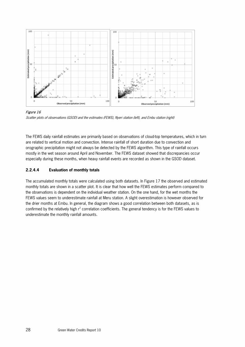
The r2 correlation coefficient for the three stations ranges from 0.28 (Nyeri) to 0.47 (Meru). Discrepancies can be found in the Nyeri datasets, especially for the large rainfall events. The correlation coefficient is strongly affected by these discrepancies, and consequently the coefficient is relatively low for this station - while in the scatter plot a very clear correlation can be observed (Figure 16), although FEWS slightly underestimates the actual values.
28 Green Water Credits Report 10
Figure 16
Scatter plots of observations (GSOD) and the estimates (FEWS), Nyeri station (left), and Embu station (right)
The FEWS daily rainfall estimates are primarily based on observations of cloud-top temperatures, which in turn are related to vertical motion and convection. Intense rainfall of short duration due to convection and orographic precipitation might not always be detected by the FEWS algorithm. This type of rainfall occurs mostly in the wet season around April and November. The FEWS dataset showed that discrepancies occur especially during these months, when heavy rainfall events are recorded as shown in the GSOD dataset. 2.2.4.4 Evaluation of monthly totals
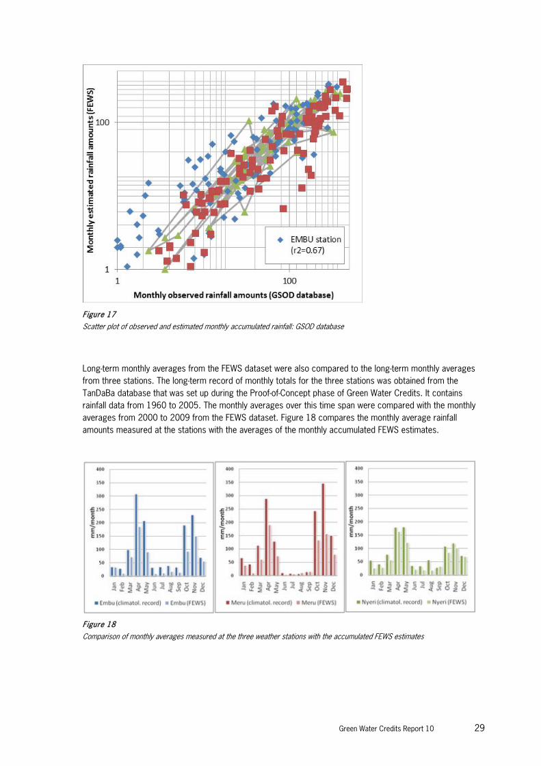
The accumulated monthly totals were calculated using both datasets. In Figure 17 the observed and estimated monthly totals are shown in a scatter plot. It is clear that how well the FEWS estimates perform compared to the observations is dependent on the individual weather station. On the one hand, for the wet months the FEWS values seem to underestimate rainfall at Meru station. A slight overestimation is however observed for the drier months at Embu. In general, the diagram shows a good correlation between both datasets, as is confirmed by the relatively high r2 correlation coefficients. The general tendency is for the FEWS values to underestimate the monthly rainfall amounts.
Green Water Credits Report 10 29
Figure 17
Scatter plot of observed and estimated monthly accumulated rainfall: GSOD database
Long-term monthly averages from the FEWS dataset were also compared to the long-term monthly averages from three stations. The long-term record of monthly totals for the three stations was obtained from the TanDaBa database that was set up during the Proof-of-Concept phase of Green Water Credits. It contains rainfall data from 1960 to 2005. The monthly averages over this time span were compared with the monthly averages from 2000 to 2009 from the FEWS dataset. Figure 18 compares the monthly average rainfall amounts measured at the stations with the averages of the monthly accumulated FEWS estimates.
Figure 18
Comparison of monthly averages measured at the three weather stations with the accumulated FEWS estimates

30 Green Water Credits Report 10
In general, both data sources show the same precipitation regime over the year, at each of the weather station locations. However the differences between the observed and estimated averages are especially apparent during the wet months. It confirms that the FEWS algorithm does not detect all the heavy rainfall events and that for this reason the monthly averages are lower than those from the climatological record. Also, a careful look at the daily data shows that some local heavy rainfall events are not represented in the FEWS dataset. This seasonal effect can also be observed by analysing the residual mean - defined as the average difference between the observed values from the weather stations and the estimated values of the FEWS grids. Figure 19 shows the residual mean for every month in the time series, to give an insight into the difference between observation and estimate on a monthly basis. It can be observed that the differences are evident, particularly during the rainy months. Moreover, the difference between datasets is almost always negative, which means that on average the FEWS estimates have lower values than the observed GSOD dataset.
Figure 19
Residual (estimate - observed) mean per month of the three stations
Winds with an easterly component dominate the Kenyan tropics. The north-easterly monsoons are most prevalent from December to April while the south-easterly monsoon dominates from April to October (Gatebe et al. 1999). The monthly accumulated FEWS grids (Figure 20) show that the orographic precipitation caused by these winds is detected on the west side of Mount Kenya. Around the Aberdare mountain range this orographic effect is lower as can be observed in Figure 20.

Green Water Credits Report 10 31
Figure 20
Monthly total for April 2002 from the FEWS rainfall estimations
1.1.1.1 Evaluation of annual totals
A comparison between FEWS and GSOD annual totals was also made. The daily datasets were used to obtain the yearly accumulated total rainfall amounts for each of the three weather stations, and for the corresponding pixels from the FEWS gridded estimates. The years that contained too many missing values were filtered out, depending on whether the missing values were recorded during a wet or a dry period during the year. Figure 21 presents the results for both datasets for the years 2001, 2002, 2006, 2007 and 2008.
Figure 21
Observed (GSOD) and estimated (FEWS) yearly total rainfall amounts for Meru station
32 Green Water Credits Report 10
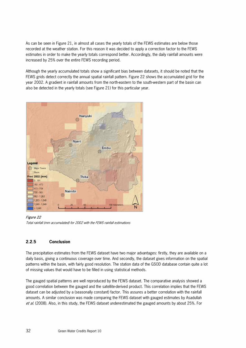
As can be seen in Figure 21, in almost all cases the yearly totals of the FEWS estimates are below those recorded at the weather station. For this reason it was decided to apply a correction factor to the FEWS estimates in order to make the yearly totals correspond better. Accordingly, the daily rainfall amounts were increased by 25% over the entire FEWS recording period. Although the yearly accumulated totals show a significant bias between datasets, it should be noted that the FEWS grids detect correctly the annual spatial rainfall pattern. Figure 22 shows the accumulated grid for the year 2002. A gradient in rainfall amounts from the north-eastern to the south-western part of the basin can also be detected in the yearly totals (see Figure 21) for this particular year.
Figure 22
Total rainfall (mm accumulated) for 2002 with the FEWS rainfall estimations
2.2.5 Conclusion
The precipitation estimates from the FEWS dataset have two major advantages: firstly, they are available on a daily basis, giving a continuous coverage over time. And secondly, the dataset gives information on the spatial patterns within the basin, with fairly good resolution. The station data of the GSOD database contain quite a lot of missing values that would have to be filled in using statistical methods. The gauged spatial patterns are well reproduced by the FEWS dataset. The comparative analysis showed a good correlation between the gauged and the satellite-derived product. This correlation implies that the FEWS dataset can be adjusted by a (seasonally constant) factor. This assures a better correlation with the rainfall amounts. A similar conclusion was made comparing the FEWS dataset with gauged estimates by Asadullah et al. (2008). Also, in this study, the FEWS dataset underestimated the gauged amounts by about 25%. For

Green Water Credits Report 10 33
Green Water Credits, the dataset was adjusted by a factor of 1.25, leading to an excellent correspondence with the gauged dataset. The remaining required data for the SWAT model, namely temperature, solar radiation, wind velocity and relative humidity, were obtained from the stations through the GSOD database. The temperature lapse rate was set to -6oC/km. These meteorological data are available on a daily time scale. Therefore, there is sufficient information to apply the Penman-Monteith method in the model to determine the potential evapotranspiration rates, leading to better estimates of this negative term of the basin water balance. 2.3 Land cover
2.3.1 Data sources
2.3.1.1 The Africover dataset
The GWC Phase I studies used the best available maps, based on the FAO Africover project (FAO 2000) which designates land use/land cover for points on an approximately 2400 x 4800 m irregular grid. The effective scale is about 1: 250,000. The land cover was produced from visual interpretation of digitally enhanced LANDSAT TM images (Bands 4,3,2) acquired mainly in the year 1999. The land cover classes were developed using the FAO/UNEP international standard Land Cover Classification System (LCCS). 2.3.1.2 The GlobCover dataset
GlobCover is an ESA initiative in partnership with JRC, EEA, FAO, UNEP, GOFC-GOLD and IGBP. The GlobCover project has developed a service capable of delivering global composite and land cover maps using, as input, observations from the 300 m MERIS sensor on board the ENVISAT satellite mission. The GlobCover service was demonstrated over a period of 19 months (December 2004 - June 2006), for which a set of MERIS Full Resolution (FR) composites (bi-monthly and annual) and a Global Land Cover map are being produced. The GlobCover composites are derived from the MERIS FR images such as cloud detection, atmospheric correction, geolocalisation and re-mapping. The GlobCover Land Cover map is compatible with the UN Land Cover Classification System (LCCS). The use of medium resolution data provides a considerable improvement in comparison with other global land cover products at lower spatial resolution - for example the GLC2000 dataset. However, the quality of the GlobCover product is closely dependent on the reference land cover database used for the labelling process, and on the number of valid observations available as input. When the reference dataset is of higher spatial resolution with good thematic detail, the GlobCover product also shows high accuracy. On the other hand, the number of valid observations is a constraint. The spatial coverage of the MERIS data clearly determines the quality of the temporal mosaics and, therefore, of the land cover map. 2.3.2 Dataset evaluation
The Africover and GlobCover dataset were produced using different methods and different sources of remote sensing information. A major difference is that the classification of the Africover dataset was based on visual interpretation of the satellite imagery, while the GlobCover dataset used an automated classification approach using local reference datasets. In order to evaluate which of the two datasets is optimal for the hydrological model, both datasets were analysed and compared with recent high resolution satellite imagery.
34 Green Water Credits Report 10
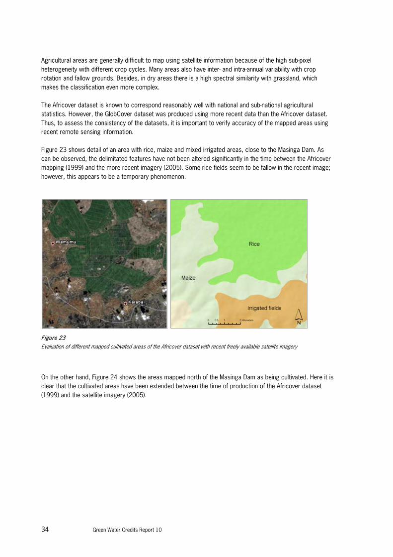
Agricultural areas are generally difficult to map using satellite information because of the high sub-pixel heterogeneity with different crop cycles. Many areas also have inter- and intra-annual variability with crop rotation and fallow grounds. Besides, in dry areas there is a high spectral similarity with grassland, which makes the classification even more complex. The Africover dataset is known to correspond reasonably well with national and sub-national agricultural statistics. However, the GlobCover dataset was produced using more recent data than the Africover dataset. Thus, to assess the consistency of the datasets, it is important to verify accuracy of the mapped areas using recent remote sensing information. Figure 23 shows detail of an area with rice, maize and mixed irrigated areas, close to the Masinga Dam. As can be observed, the delimitated features have not been altered significantly in the time between the Africover mapping (1999) and the more recent imagery (2005). Some rice fields seem to be fallow in the recent image; however, this appears to be a temporary phenomenon.
Figure 23
Evaluation of different mapped cultivated areas of the Africover dataset with recent freely available satellite imagery
On the other hand, Figure 24 shows the areas mapped north of the Masinga Dam as being cultivated. Here it is clear that the cultivated areas have been extended between the time of production of the Africover dataset (1999) and the satellite imagery (2005).
Green Water Credits Report 10 35
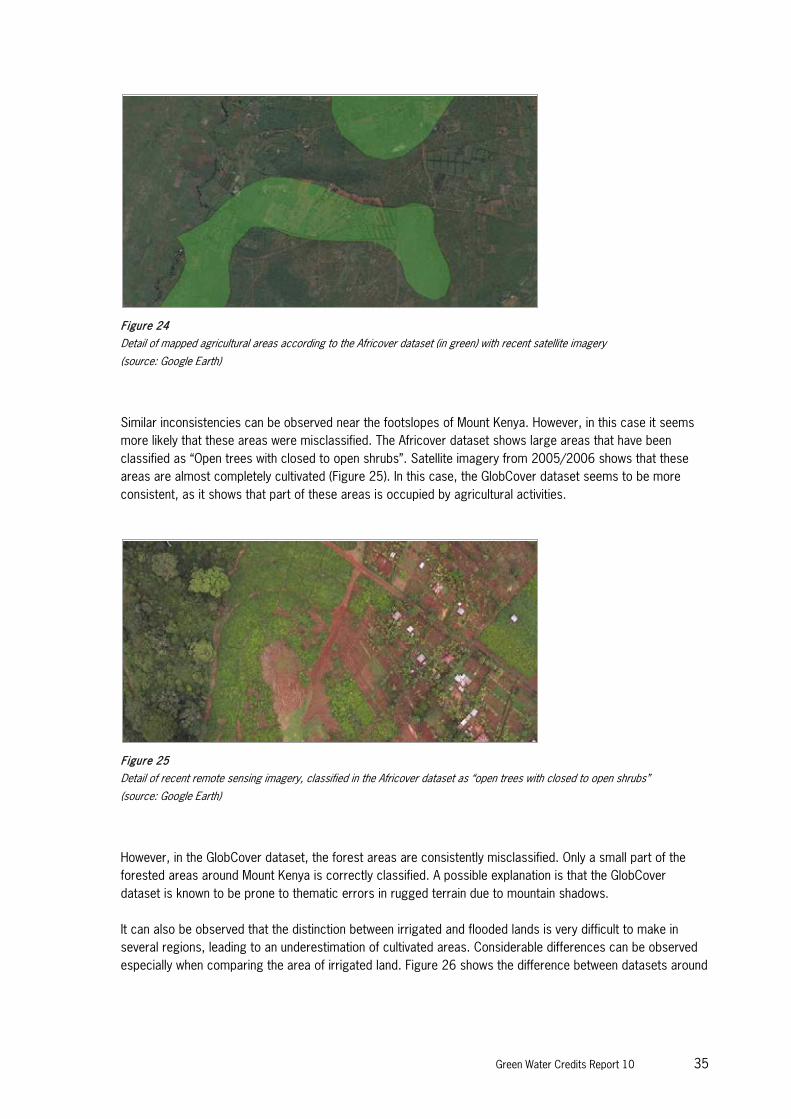
Figure 24
Detail of mapped agricultural areas according to the Africover dataset (in green) with recent satellite imagery
(source: Google Earth)
Similar inconsistencies can be observed near the footslopes of Mount Kenya. However, in this case it seems more likely that these areas were misclassified. The Africover dataset shows large areas that have been classified as “Open trees with closed to open shrubs”. Satellite imagery from 2005/2006 shows that these areas are almost completely cultivated (Figure 25). In this case, the GlobCover dataset seems to be more consistent, as it shows that part of these areas is occupied by agricultural activities.
Figure 25
Detail of recent remote sensing imagery, classified in the Africover dataset as “open trees with closed to open shrubs”
(source: Google Earth)
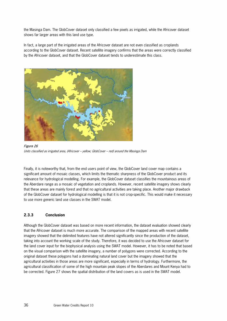
However, in the GlobCover dataset, the forest areas are consistently misclassified. Only a small part of the forested areas around Mount Kenya is correctly classified. A possible explanation is that the GlobCover dataset is known to be prone to thematic errors in rugged terrain due to mountain shadows. It can also be observed that the distinction between irrigated and flooded lands is very difficult to make in several regions, leading to an underestimation of cultivated areas. Considerable differences can be observed especially when comparing the area of irrigated land. Figure 26 shows the difference between datasets around
36 Green Water Credits Report 10
the Masinga Dam. The GlobCover dataset only classified a few pixels as irrigated, while the Africover dataset shows far larger areas with this land use type. In fact, a large part of the irrigated areas of the Africover dataset are not even classified as croplands according to the GlobCover dataset. Recent satellite imagery confirms that the areas were correctly classified by the Africover dataset, and that the GlobCover dataset tends to underestimate this class.
Figure 26
Units classified as irrigated area, (Africover – yellow; GlobCover – red) around the Masinga Dam
Finally, it is noteworthy that, from the end users point of view, the GlobCover land cover map contains a significant amount of mosaic classes, which limits the thematic sharpness of the GlobCover product and its relevance for hydrological modelling. For example, the GlobCover dataset classifies the mountainous areas of the Aberdare range as a mosaic of vegetation and croplands. However, recent satellite imagery shows clearly that these areas are mainly forest and that no agricultural activities are taking place. Another major drawback of the GlobCover dataset for hydrological modelling is that it is not crop-specific. This would make it necessary to use more generic land use classes in the SWAT model. 2.3.3 Conclusion
Although the GlobCover dataset was based on more recent information, the dataset evaluation showed clearly that the Africover dataset is much more accurate. The comparison of the mapped areas with recent satellite imagery showed that the delimited features have not altered significantly since the production of the dataset, taking into account the working scale of the study. Therefore, it was decided to use the Africover dataset for the land cover input for the biophysical analysis using the SWAT model. However, it has to be noted that based on the visual comparison with the satellite imagery, a number of polygons were corrected. According to the original dataset these polygons had a dominating natural land cover but the imagery showed that the agricultural activities in those areas are more significant, especially in terms of hydrology. Furthermore, the agricultural classification of some of the high mountain peak slopes of the Aberdares and Mount Kenya had to be corrected. Figure 27 shows the spatial distribution of the land covers as is used in the SWAT model.

Green Water Credits Report 10 37
Figure 27
Land cover map as used in the SWAT model, main source: Africover dataset, corrected by comparison with recent satellite imagery
2.4 Soils
2.4.1 Data sources
2.4.1.1 The KENSOTER database
The KENSOTER database at the scale of 1:1 million (KSS 1996) holds data on landform, parent material and soils in a standardised digital format (van Engelen and Wen 1995). The database was updated by the Kenya Soil Survey (KSS) and ISRIC-World Soil Information (Batjes and Gicheru 2004). This 2004 version was expanded for GWC by additional profile data with measured water retention values of the Upper Tana catchment. The current KENSOTER database now contains data of 340 soil profiles, of which 68 are from the Upper Tana: this is referred to as the KENSOTER-version 2 database (KSS and ISRIC 2007). The dominant soil types of the Upper Tana catchment are presented in Figure 28, and show a relationship with elevation. The higher slopes of Mt Kenya and the Aberdares are dominated by volcanic ash soils (Andosols). The middle footslopes have mainly deep, well-structured nutrient-rich clay soils (Nitisols). The lower footslopes are dominated by very deep, strongly leached, poor clay soils (Ferralsols) and by less leached soils (Cambisols and Luvisols). At lower elevations, roughly below 1000m, Cambisols and sodic-alkaline soils (Solonetz) are dominant (KSS 1996; Sombroek et al. 1982).

38 Green Water Credits Report 10
Figure 28
Dominant soil types of the Upper Tana catchment (KENSOTER-version 2)
Effective rootable depth and Available Water Content4 are key soil hydrological properties determining the water balance, as used in SWAT (Table 5). The geographic distribution and the differences are shown in Figure 29 and Figure 30. Comparing soil types in the Upper Tana it appears there is a factor of 5 to 10 difference between lowest and highest values of Total Available Water Content.
4 Available Water Content is the amount of moisture held between pF2.3 and pF4.2

Green Water Credits Report 10 39
Table 5
Average soil moisture characteristics of dominant soils in the Upper Tana catchment
Dominant soil (and phase)
Effective rootable depth
(cm)
Moisture at saturation
(%)(a)
Moisture at Field Capacity (%)
Moisture at Wilting Point
(%)
Available Water Content(b)
(%)
Total Available Water(c)
(mm)
Acrisols 113 56 24 16 9 98 Andosols 100 60 40 24 16 172 Arenosols 100 53 16 3 13 130 Chernozems 75 55 37 21 16 120 Calcisols 40 41 16 10 6 24 Cambisols 53 48 28 14 14 74 Fluvisols 93 44 17 4 13 120 Ferralsols 90 53 26 17 9 82 Gleysols 45 56 37 21 16 72 Leptosols 10 53 21 12 9 7 Luvisols 80 47 25 13 12 95 Lixisols 88 47 16 11 5 43 Nitisols 104 53 31 22 9 98 Phaeozems 80 56 38 26 12 98 Planosols 25 50 35 22 13 33 Regosols 37 48 19 9 10 33 Solonetzs 28 45 28 13 15 42 Vertisols 80 50 46 22 24 191
Volume percentages; (b) Available water or plant extractable water; (c) Total available water = Available Water Content over Effective rooting depth.
Figure 29
Available Water Capacity of dominant soils of the Upper and Middle Tana catchments (KENSOTER-version 2)

40 Green Water Credits Report 10
Figure 30
Rootable depth of dominant soils of the Upper and Middle Tana catchments (KENSOTER-version 2)
2.4.1.2 Harmonised KENSOTER
The harmonised KENSOTER database is a secondary dataset with median attribute values. Missing entries are based on pedotransfer rules (van Engelen et al. 2005). Following these taxotransfer rules (Batjes 2003), the median attribute values were estimated using attribute data and aggregated over five fixed depth intervals, all on the basis of texture group and soil unit classification. Soil classification follows the Revised Legend of the Soil Map of the World. The harmonised KENSOTER database includes the total available water capacity of the soil, which data can be directly used in SWAT. A comparison of the two databases showed that the soil moisture contents given by the harmonised KENSOTER database are higher than those of the measured data in the KENSOTER-version 2 database. The rootable soil depth is directly extracted from the harmonised KENSOTER database. In a few cases the rootable depths of the harmonised KENSOTER is somewhat different to the KENSOTER-version 2, because of the use of different criteria. The harmonised KENSOTER database contains most of the information necessary for the SWAT model: therefore, it is convenient to use it also for the model input on soil characteristics, although some of the properties were derived and not fully consistent with the measured values. 2.4.1.3 Pedotransfer functions
An important characteristic not provided in the KENSOTER database is the saturated hydraulic conductivity. A well-developed technique to overcome this problem is to use pedotransfer functions (PTF). A wide range of pedotransfer functions have been developed and applied successfully over the last decades over various scales e.g. field scale (Droogers et al. 2001) and basin scale (Droogers and Kite 2001).

Green Water Credits Report 10 41
Sobieraj et al. (2001) concluded from a detailed analysis that most PTFs were not very reliable and that the impact on runoff estimates could be considerable. The PTF that generated conductivity values close to measured ones was the Jabro equation (Jabro 1992): Ksat = exp(11.86 – 0.81 log(st) – 1.09 log(cl) – 4.64 BD) Ksat = saturated hydraulic conductivity (cm h-1) st = silt content (%) cl = clay content (%) This equation was used to derive Ksat values from the KENSOTER database. 2.4.2 Conclusion
SWAT requires detailed spatially distributed information on soil characteristics and related soil parameters. The information available in the harmonised KENSOTER database was found to be adequate for use in the SWAT model. The saturated hydraulic conductivity was obtained using the described methodology by means of pedotransfer functions. 2.5 Streamflow
2.5.1 Data source
Discharge data of only a few streamflow gauges were available in the study area. Figure 31 shows the locations of gauging stations in the Upper Tana. Figure 31 and Table 6 provide an overview of the gauging stations data that were obtained and processed. Data were made available by the Kenyan Soil Survey, the University of Nairobi and some additional data came from the Global Runoff Discharge Database. The most complete series of observed streamflow data is from 1962-1977 (see Table 6). 2.5.2 Dataset evaluation
Data quality was poor, with missing records, unknown units, and locations, and conflicting names, etc. An example is station 4CC05 which is the inflow from Thika River in Masinga. A total of 15 years (1966-1980) of daily data were available. Of the total 5479 records, 1340 were missing - corresponding to almost 25%.

42 Green Water Credits Report 10
Figure 31
Locations of gauging stations from which data were obtained
Data accuracy can also be hampered by the source of data. One example is the Garissa station, the outlet point of the Middle Tana, where daily data were obtained from two sources (University of Nairobi and Global River Discharge Database). Data from UoN were daily records from 1941 to 1993, and data from GRDD covered 1934 to 1975, on a monthly basis. Figure 32 shows the difference between these two data sources for the overlapping period (1941 to 1975). The scatter plot in Figure 32 indicates that considerable differences exist between the two datasets. The time plot, however, reveals that patterns are quite comparable, and peak and low flows are especially comparable for the two datasets. For the streamflow station at Grand Falls, known as 4F13, two records of data were obtained from two different data sources as well (Figure 33). For these two datasets some differences also occur, but these differences were restricted to some periods in the 1960s and 1970s. Besides data from gauging stations, reservoir data on inflow and outflow were available from various sources (University of Nairobi and KenGen). For Masinga, both inflow and outflow data were available; while for the other reservoirs (Kamburu, Gitaru, Kindaruma and Kiambere) only inflow levels were obtained. Flow data is available from either stream gauges (Table 6) or from reservoir measurements (Table 7). The location of the gauges is given in Figure 31.
Green Water Credits Report 10 43
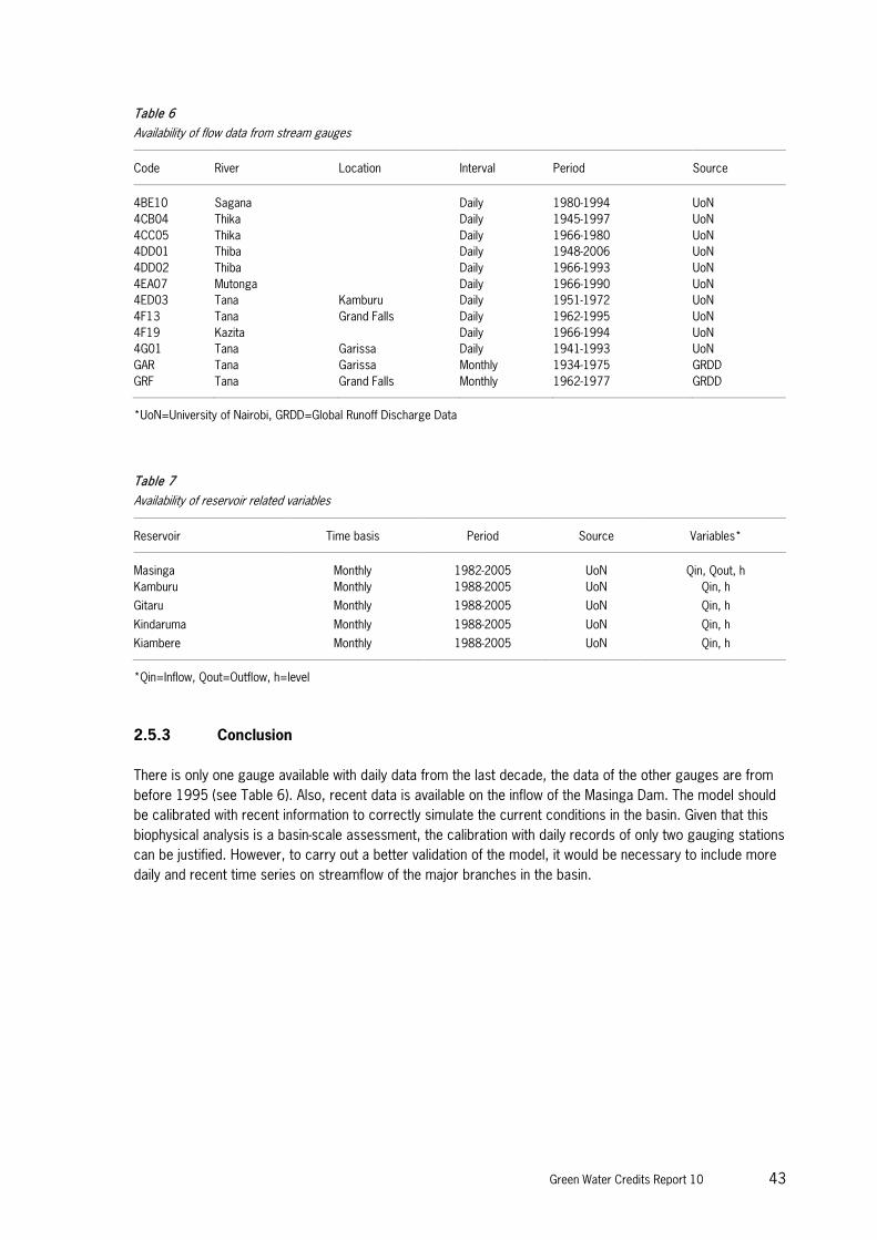
Table 6
Availability of flow data from stream gauges
Code River Location Interval Period Source
4BE10 Sagana Daily 1980-1994 UoN 4CB04 Thika Daily 1945-1997 UoN 4CC05 Thika Daily 1966-1980 UoN 4DD01 Thiba Daily 1948-2006 UoN 4DD02 Thiba Daily 1966-1993 UoN 4EA07 Mutonga Daily 1966-1990 UoN 4ED03 Tana Kamburu Daily 1951-1972 UoN 4F13 Tana Grand Falls Daily 1962-1995 UoN 4F19 Kazita Daily 1966-1994 UoN 4G01 Tana Garissa Daily 1941-1993 UoN GAR Tana Garissa Monthly 1934-1975 GRDD GRF Tana Grand Falls Monthly 1962-1977 GRDD
*UoN=University of Nairobi, GRDD=Global Runoff Discharge Data
Table 7
Availability of reservoir related variables
Reservoir Time basis Period Source Variables*
Masinga Monthly 1982-2005 UoN Qin, Qout, h Kamburu Monthly 1988-2005 UoN Qin, h
Gitaru Monthly 1988-2005 UoN Qin, h
Kindaruma Monthly 1988-2005 UoN Qin, h
Kiambere Monthly 1988-2005 UoN Qin, h
*Qin=Inflow, Qout=Outflow, h=level
2.5.3 Conclusion
There is only one gauge available with daily data from the last decade, the data of the other gauges are from before 1995 (see Table 6). Also, recent data is available on the inflow of the Masinga Dam. The model should be calibrated with recent information to correctly simulate the current conditions in the basin. Given that this biophysical analysis is a basin-scale assessment, the calibration with daily records of only two gauging stations can be justified. However, to carry out a better validation of the model, it would be necessary to include more daily and recent time series on streamflow of the major branches in the basin.

44 Green Water Credits Report 10
Figure 32
Comparison between similar data from two sources at Garissa. GAR originates from Global Runoff Discharge Data and 4G01 from
the University of Nairobi
0
200
400
600
800
1000
1200
0
200
400
600
800
1000
1200
GAR flow (m3/s)
4G01
flow
(m3/
s)
0
200
400
600
800
1000
1200
1400
1600
1800
2000
1941
1943
1945
1947
1949
1951
1953
1955
1957
1959
1961
1963
1965
1967
1969
1971
1973
1975
Flow
(m3/
s)
GAR4G01

Green Water Credits Report 10 45
Figure 33
Comparison between similar data from two sources at Grand Falls. GRF originates from Global Runoff Discharge Data and 4F13
from the University of Nairobi
0
200
400
600
800
1000
1200
0
200
400
600
800
1000
1200
GRF flow (m3/s)
4F13
flow
(m3/
s)
0
200
400
600
800
1000
1200
1400
1600
1800
2000
1962
1964
1966
1968
1970
1972
1974
1976
1978
1980
1982
1984
1986
1988
1990
1992
1994
Flow
(m3/
s)
GRF4F13
46 Green Water Credits Report 10
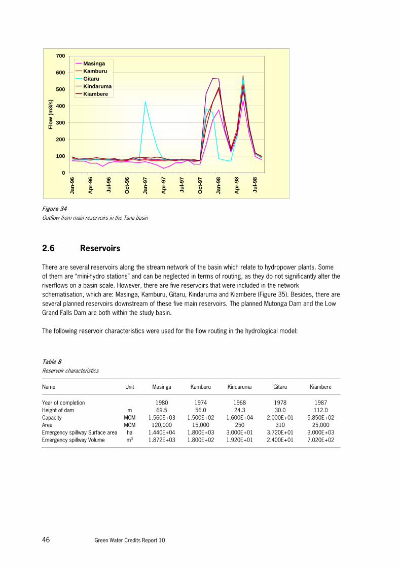
Figure 34
Outflow from main reservoirs in the Tana basin
2.6 Reservoirs
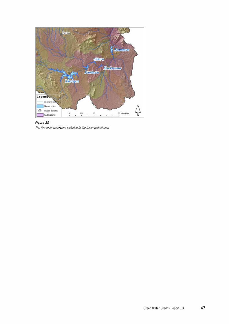
There are several reservoirs along the stream network of the basin which relate to hydropower plants. Some of them are “mini-hydro stations” and can be neglected in terms of routing, as they do not significantly alter the riverflows on a basin scale. However, there are five reservoirs that were included in the network schematisation, which are: Masinga, Kamburu, Gitaru, Kindaruma and Kiambere (Figure 35). Besides, there are several planned reservoirs downstream of these five main reservoirs. The planned Mutonga Dam and the Low Grand Falls Dam are both within the study basin. The following reservoir characteristics were used for the flow routing in the hydrological model:
Table 8
Reservoir characteristics
Name Unit Masinga Kamburu Kindaruma Gitaru Kiambere
Year of completion 1980 1974 1968 1978 1987 Height of dam m 69.5 56.0 24.3 30.0 112.0 Capacity MCM 1.560E+03 1.500E+02 1.600E+04 2.000E+01 5.850E+02 Area MCM 120,000 15,000 250 310 25,000 Emergency spillway Surface area ha 1.440E+04 1.800E+03 3.000E+01 3.720E+01 3.000E+03 Emergency spillway Volume m3 1.872E+03 1.800E+02 1.920E+01 2.400E+01 7.020E+02
0
100
200
300
400
500
600
700
Jan-
96
Apr
-96
Jul-9
6
Oct
-96
Jan-
97
Apr
-97
Jul-9
7
Oct
-97
Jan-
98
Apr
-98
Jul-9
8
Flow
(m3/
s)
MasingaKamburuGitaruKindarumaKiambere
Green Water Credits Report 10 47
Figure 35
The five main reservoirs included in the basin delimitation

48 Green Water Credits Report 10

Green Water Credits Report 10 49
3 Baseline model analysis
3.1 Introduction
The Proof-of-Concept phase of Green Water Credits showed that the Soil and Water Assessment Tool (SWAT) was appropriate to study, and quantify, the up- and downstream interactions in the basin, as well as the influence of land use and management on the water resources and sediment transport in the basin. For the current operational design phase a more accurate model was set up using the best available data sources, as discussed in Chapter Model revision5. The model was set up with data from the last 10 years (2000 to 2009) in order to obtain insight into the current basin situation and interactions. This is an improvement compared to the Proof-of-Concept phase, when historical datasets were used for the basin assessment. The main goal of this assessment is to quantify the impact of Green Water Credits management practices and to identify potential pilot areas from a biophysical point of view. This impact on the water and sediment balances in the basin depends on the water it receives through precipitation. For this reason, it is useful to assess the impact both during a dry and a wet year -and thus to focus on the wettest and driest years of the 10-year time series in order to obtain insight into the effectiveness of management options during both extremes. From the last ten years, 2005 represents the last year of a short drought period that started in 2004 (Figure 36). On the other hand, 2006 can be considered an extraordinarily wet year with about twice the rainfall of 2005. These two years were used to quantify how the different Green Water Credits management options affect the green and blue water resources in the basin.
Figure 36
Total yearly basin rainfall (FEWS precipitation estimates)

50 Green Water Credits Report 10
3.2 Model set up
3.2.1 Distributed model input
The evaluation of the available data sources on precipitation (Chapter 2.2) indicated that the use of the FEWS dataset implies a considerable improvement compared to the use of point data from the weather stations, as was carried out during the Proof-of-Concept phase. This dataset was therefore used as the forcing weather model input, after a bias correction with the observed weather station data. Other meteorological data required by the model such as temperature, wind, radiation, etc. were obtained from the measured time series at the three available weather stations in the basin. For the daily temperature throughout the basin a lapse rate of -6oC/km was used. The FEWS dataset gives a reliable estimate of the spatial distribution of the daily precipitation amounts throughout the basin. The methodology used to delineate the sub-catchments allowed the correct incorporation of this information permitting a fully distributed rainfall-runoff modelling approach. The daily rainfall grids were prepared for the model input and the different daily rainfall time series were assigned to each sub-catchment in the model. For Figure 37 the daily values were summed, showing the total rainfall per sub-catchment for the dry (2005) and the wet year (2006).
Figure 37
Total precipitation for 2005 (left) and 2006 (right)
3.2.2 Hydrological response units
For the spatial delineation of the sub-catchments, SWAT uses the concept of Hydrological Response Units (HRU) (Neitsch et al. 2002): portions of a sub-catchment that possess unique land use/management/soil attributes. In other words, an HRU is the total area in the sub-catchment with a particular land use, management and soil combination. While individual fields with a specific land use, management and soil may be scattered throughout a sub-catchment, these areas are lumped together to form one HRU. HRUs are used in SWAT runs since they simplify the process of identifying single response units. The size of a HRU depends on the size of the total area under consideration. Implicit in the concept of the HRU is the assumption that there is no interaction between HRUs in one sub-catchment. Loadings (runoff with sediment, nutrients, etc. transported by the runoff) from each HRU are

Green Water Credits Report 10 51
calculated separately and then summed together to determine the total loadings from the sub-catchment. If the interaction of one land use area with another is significant, rather than defining those land use areas as HRUs, they should be defined as sub-catchments. It is only at the sub-catchment level that spatial relationships can be specified. The benefit of HRUs is the increase in accuracy it adds to the prediction of loadings from the sub-catchment. The growth and development of plants can differ greatly among species. When the diversity in plant cover within a sub-basin is accounted for, the net amount of runoff entering the main channel from the sub-catchment will be much more accurate. In practice the HRUs are defined by overlaying three data layers: (i) sub-catchments, (ii) land cover (section 2.3Fout! Verwijzingsbron niet gevonden.), and (iii) soils (section 2.4). Due to computational constraints it is necessary to limit the total number of HRUs, and to filter out the minor land use and soil classes within each sub-catchment. For this analysis, a threshold of 10% for both layers was used. This means that if a certain land use and soil combination covers less than 10% in a certain sub-catchment, the HRU in question was filtered out. This way, only the dominating units in terms of hydrological response within each sub-catchment are analysed. A total of 2226 HRUs were determined using this procedure (Figure 38) which means a substantial improvement to the Proof-of-Concept model when 874 HRUs were defined, distributed over a larger basin (outlet Garissa).
Figure 38
The hydrological response units defined (HRUs)
3.3 Calibration and model performance
The FEWS precipitation estimates were available from the year 2000 (October) until 2009 (April). Measured riverflow data were available until 2005 for two very relevant points in the basin. Additional calibration including

52 Green Water Credits Report 10
more gauged points is scheduled to take place in a follow-up study. For the pilot operation of Green Water Credits, the key focus is to assess the impact of the GWC practices on the water and sediment fluxes in the basin, quantifying the differences between the studied scenarios and the current management situation (i.e. the baseline scenario). In this context, it is crucial to note that conclusions drawn from scenario analyses are much more reliable than absolute model predictions (relative vs. absolute model accuracy, e.g. Droogers et al. 2008). To determine the calibration parameters, a sensitivity analysis was first carried out, using the parameters shown in Table 9. These five parameters were altered within realistic boundary conditions, showing that the model output was most responsive to soil available water capacity and the groundwater delay time. The second parameter determines the time lag between the moment the water leaves soil storage and the moment it becomes available in the aquifer storage. It is difficult to infer this parameter from measurable soil and hydro-geological characteristics, especially at the basin scale. Also, the soil available water capacity is a parameter which is known to be highly heterogeneous.
Table 9
Parameters used for sensitivity analysis
SWAT Code Unit Variable
Alpha_BF Days Baseflow alpha factor
GW_REVAP - Groundwater "revap" coefficient
SOL_AWC mm H20/mm soil Available water capacity of the soil layer
GW_DELAY Days Groundwater delay time
SOL_K mm/hr Saturated hydraulic conductivity
The soil available water capacity and the groundwater delay time were used to calibrate the model. It was assumed that the a priori estimates of these parameters represent the spatial distribution pattern, but that the relative magnitudes of the parameters in each field need to be adjusted up or down via a single multiplier α. This is a common method to calibrate distributed hydrological models (e.g. Vieux et al. 2004). The following table shows the values of α used for the calibration:
Table 10
Boundary values and calibrated value of multiplier used for calibration
Parameter α lower limit α upper limit α final
GW_REVAP 0.03 1.5 0.3
SOL_AWC 0.3 1.5 1
The calibration was done using the daily observations at the two gauges, each of them at a key location within the basin. The two gauges are located upstream of the reservoirs, which guarantees that streamflow reaching the gauges is not influenced by reservoir operations. Moreover, they allow the calibration of the two major parts of the basin. The data available on the inflow to the Masinga reservoir effectively covers the two major
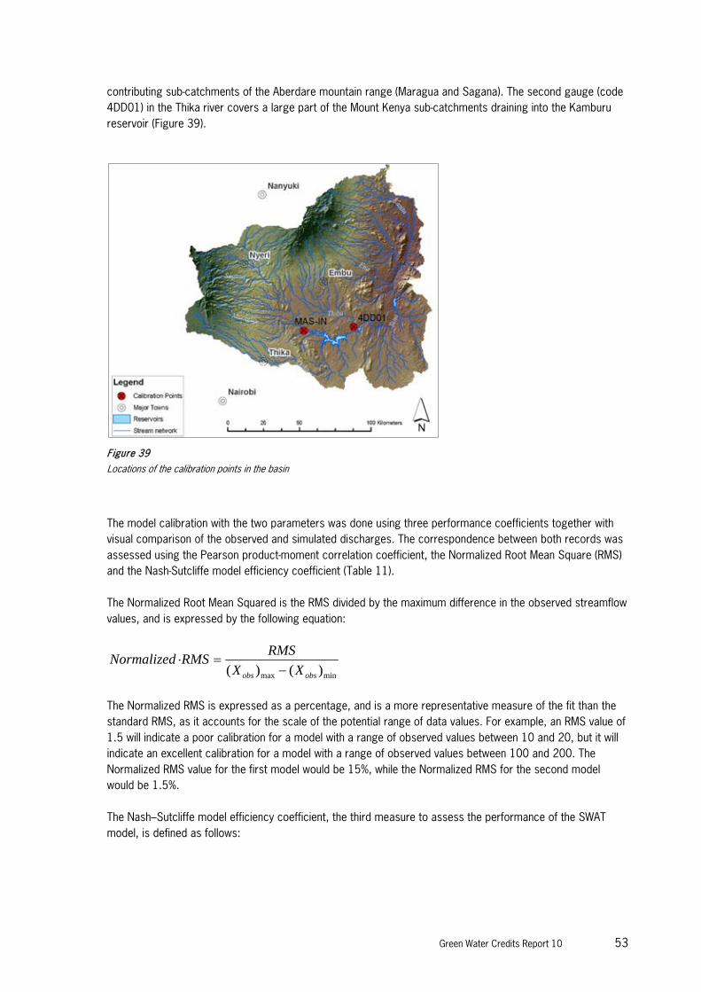
Green Water Credits Report 10 53
contributing sub-catchments of the Aberdare mountain range (Maragua and Sagana). The second gauge (code 4DD01) in the Thika river covers a large part of the Mount Kenya sub-catchments draining into the Kamburu reservoir (Figure 39).
Figure 39
Locations of the calibration points in the basin
The model calibration with the two parameters was done using three performance coefficients together with visual comparison of the observed and simulated discharges. The correspondence between both records was assessed using the Pearson product-moment correlation coefficient, the Normalized Root Mean Square (RMS) and the Nash-Sutcliffe model efficiency coefficient (Table 11). The Normalized Root Mean Squared is the RMS divided by the maximum difference in the observed streamflow values, and is expressed by the following equation:
minmax )()( obsobs XXRMSRMSNormalized−
=⋅
The Normalized RMS is expressed as a percentage, and is a more representative measure of the fit than the standard RMS, as it accounts for the scale of the potential range of data values. For example, an RMS value of 1.5 will indicate a poor calibration for a model with a range of observed values between 10 and 20, but it will indicate an excellent calibration for a model with a range of observed values between 100 and 200. The Normalized RMS value for the first model would be 15%, while the Normalized RMS for the second model would be 1.5%. The Nash–Sutcliffe model efficiency coefficient, the third measure to assess the performance of the SWAT model, is defined as follows:
54 Green Water Credits Report 10
∑∑
=
=
−
−−= T
t oto
tm
T
tto
QQE
12
21
)(
)(1
where Qo is observed discharge and Qm is modelled discharge. Qo
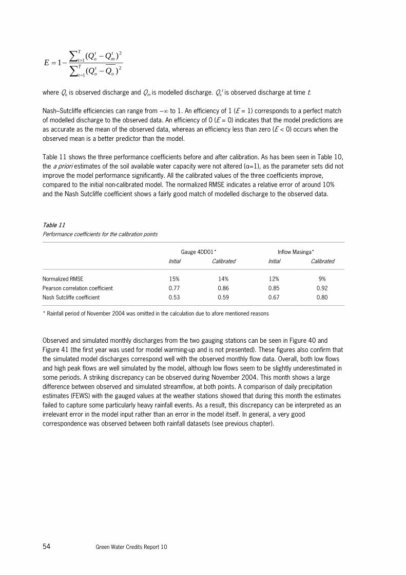
t is observed discharge at time t. Nash–Sutcliffe efficiencies can range from −∞ to 1. An efficiency of 1 (E = 1) corresponds to a perfect match of modelled discharge to the observed data. An efficiency of 0 (E = 0) indicates that the model predictions are as accurate as the mean of the observed data, whereas an efficiency less than zero (E < 0) occurs when the observed mean is a better predictor than the model. Table 11 shows the three performance coefficients before and after calibration. As has been seen in Table 10, the a priori estimates of the soil available water capacity were not altered (α=1), as the parameter sets did not improve the model performance significantly. All the calibrated values of the three coefficients improve, compared to the initial non-calibrated model. The normalized RMSE indicates a relative error of around 10% and the Nash Sutcliffe coefficient shows a fairly good match of modelled discharge to the observed data.
Table 11
Performance coefficients for the calibration points
Gauge 4DD01* Inflow Masinga*
Initial Calibrated Initial Calibrated
Normalized RMSE 15% 14% 12% 9%
Pearson correlation coefficient 0.77 0.86 0.85 0.92
Nash Sutcliffe coefficient 0.53 0.59 0.67 0.80
* Rainfall period of November 2004 was omitted in the calculation due to afore mentioned reasons
Observed and simulated monthly discharges from the two gauging stations can be seen in Figure 40 and Figure 41 (the first year was used for model warming-up and is not presented). These figures also confirm that the simulated model discharges correspond well with the observed monthly flow data. Overall, both low flows and high peak flows are well simulated by the model, although low flows seem to be slightly underestimated in some periods. A striking discrepancy can be observed during November 2004. This month shows a large difference between observed and simulated streamflow, at both points. A comparison of daily precipitation estimates (FEWS) with the gauged values at the weather stations showed that during this month the estimates failed to capture some particularly heavy rainfall events. As a result, this discrepancy can be interpreted as an irrelevant error in the model input rather than an error in the model itself. In general, a very good correspondence was observed between both rainfall datasets (see previous chapter).

Green Water Credits Report 10 55
Figure 40
Simulated and observed inflow into the Masinga reservoir
Figure 41
Simulated and observed inflow of the gauge 4DD01 (Thiba river, Kamburu reservoir)
3.4 Crop-based assessment
To explore what the most relevant land use classes regarding Green Water Credits are, results were aggregated for each land use class. The most relevant items plotted are: – The total amount of water consumed by vegetation (transpiration) and water lost by soil evaporation
(Figure 42). – T-fraction: percentage of total evapotranspiration used for vegetative transpiration (crops and other
vegetation) (green water). This factor indicates the effectiveness of the vegetation in using the green water source (Figure 43).
– Blue water: water entering the streams by surface runoff and return flow (i.e. groundwater discharge) that can be used for generating hydropower or be reused by downstream users (Figure 44).
– Erosion: total actual sediment loss (Figure 45). Evapotranspiration is the sum of water consumed by plants to grow (transpiration) and the water lost through evaporation, mainly from the soil surface (evaporation also occurs by rainfall interception but this process was not included in the analysis). Soil evaporation can be considered an unbeneficial loss of water from the system.

56 Green Water Credits Report 10
The water gained by reducing soil evaporation can be either used for crop transpiration or can infiltrate and serve as groundwater recharge.
Figure 42
Evapotranspiration split into vegetative transpiration (T) and soil evaporation (E) per crop for the dry year (2005) and the wet year
(2006) (for meaning of codes, see Figure 27)
The crops with potential to respond to implementation of green water management practices are those that are cultivated in the upstream areas. Secondly, the crops of interest should also demonstrate potential to diminish the amount of soil evaporation and reduce erosion. Figure 42 and Figure 43 give insight into what proportion of total evapotranspiration is used beneficially for the crops and how much is lost through soil evaporation. From these figures it can be concluded that the crops that show the lowest proportion currently transpired have thus the greatest potential in terms of the implementation of GWC practices. These are: – CORN: maize – COFF: coffee – AGRL: subsistence agricultural crops
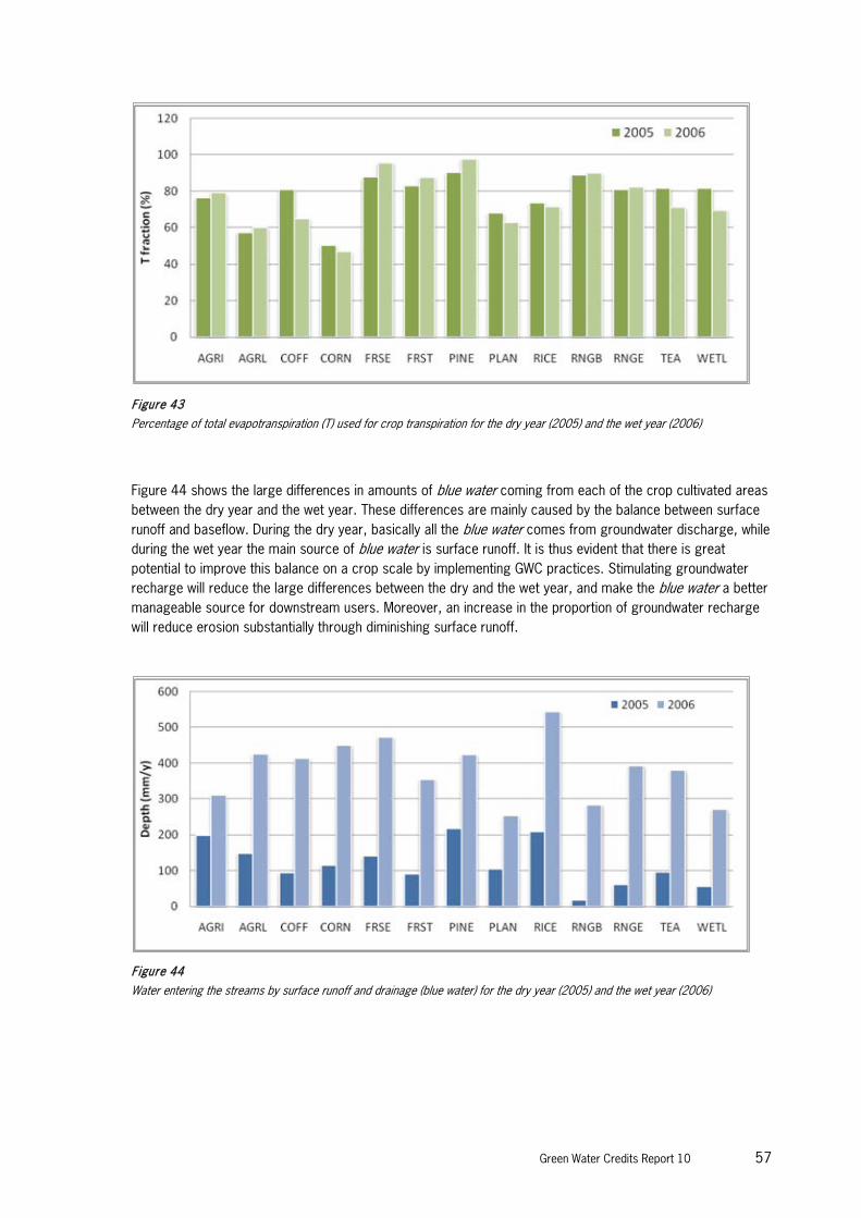
Green Water Credits Report 10 57
Figure 43
Percentage of total evapotranspiration (T) used for crop transpiration for the dry year (2005) and the wet year (2006)
Figure 44 shows the large differences in amounts of blue water coming from each of the crop cultivated areas between the dry year and the wet year. These differences are mainly caused by the balance between surface runoff and baseflow. During the dry year, basically all the blue water comes from groundwater discharge, while during the wet year the main source of blue water is surface runoff. It is thus evident that there is great potential to improve this balance on a crop scale by implementing GWC practices. Stimulating groundwater recharge will reduce the large differences between the dry and the wet year, and make the blue water a better manageable source for downstream users. Moreover, an increase in the proportion of groundwater recharge will reduce erosion substantially through diminishing surface runoff.
Figure 44
Water entering the streams by surface runoff and drainage (blue water) for the dry year (2005) and the wet year (2006)

58 Green Water Credits Report 10
As can be seen from Figure 45, the selected crops for GWC are also those that show the highest sediment loss rates, especially during the wet year. The implementation of GWC should be able to reduce erosion significantly, as is confirmed by the scenario analysis in the following chapter.
Figure 45
Total actual sediment loss per crop for the dry year (2005) and the wet year (2006)
3.5 Temporal responses
Blue water, of interest to downstream water users, is basically the sum of surface runoff and baseflow (also called return flow). Surface runoff responds immediately to rainfall events while baseflow shows a more delayed and gradual response to the rainfall events. This is an effect of the natural water reservoir of the soil and aquifer. The differences in response of both blue water sources can be clearly observed in Figure 46. The surface runoff shows peak values in the same month as the peak rainfall value, while the groundwater discharge tends to show the maximum value a month after the highest rainfall. The percolated water needs a certain travel time before it enters the aquifer storage. This storage releases its water gradually, depending on its geo-hydrological characteristics.
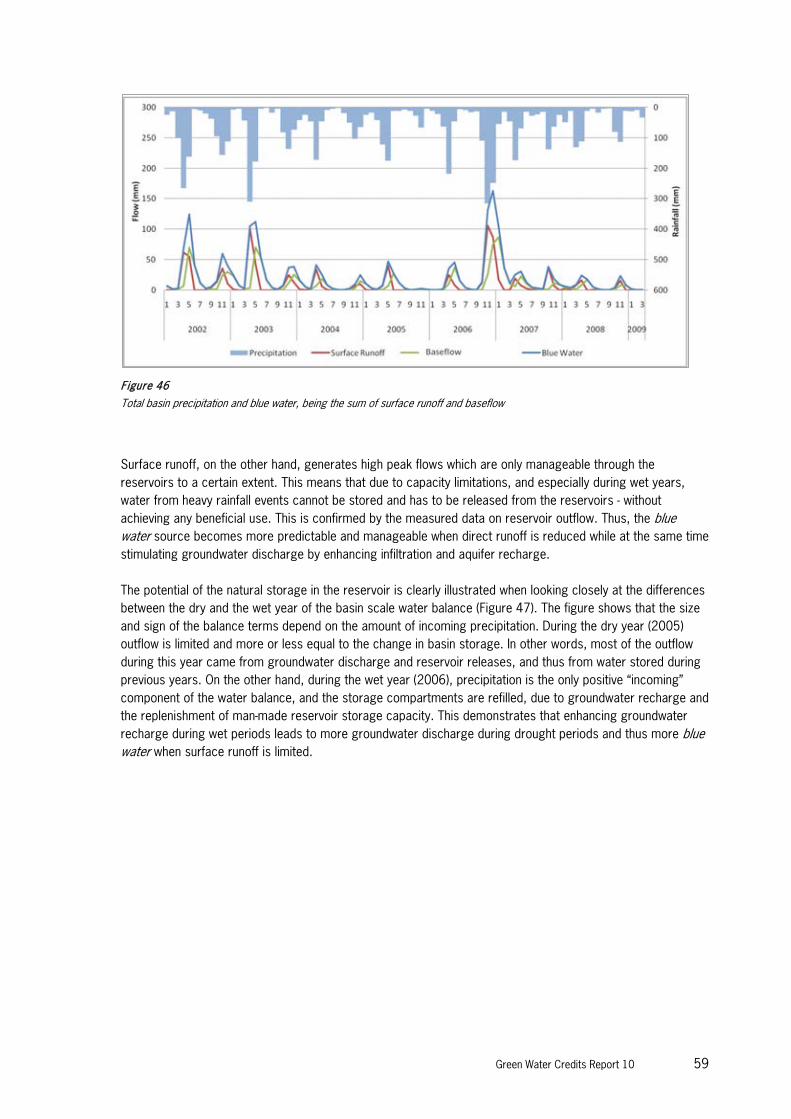
Green Water Credits Report 10 59
Figure 46
Total basin precipitation and blue water, being the sum of surface runoff and baseflow
Surface runoff, on the other hand, generates high peak flows which are only manageable through the reservoirs to a certain extent. This means that due to capacity limitations, and especially during wet years, water from heavy rainfall events cannot be stored and has to be released from the reservoirs - without achieving any beneficial use. This is confirmed by the measured data on reservoir outflow. Thus, the blue water source becomes more predictable and manageable when direct runoff is reduced while at the same time stimulating groundwater discharge by enhancing infiltration and aquifer recharge. The potential of the natural storage in the reservoir is clearly illustrated when looking closely at the differences between the dry and the wet year of the basin scale water balance (Figure 47). The figure shows that the size and sign of the balance terms depend on the amount of incoming precipitation. During the dry year (2005) outflow is limited and more or less equal to the change in basin storage. In other words, most of the outflow during this year came from groundwater discharge and reservoir releases, and thus from water stored during previous years. On the other hand, during the wet year (2006), precipitation is the only positive “incoming” component of the water balance, and the storage compartments are refilled, due to groundwater recharge and the replenishment of man-made reservoir storage capacity. This demonstrates that enhancing groundwater recharge during wet periods leads to more groundwater discharge during drought periods and thus more blue water when surface runoff is limited.

60 Green Water Credits Report 10
Figure 47
Main components of water balance during 2005 (dry) and 2006 (wet)
Figure 47 highlights the role of storage in the water balance of the basin. It is clear that the soil and aquifer reservoirs have the potential to improve the management of water resources in the basin as they assure a more continuous and reliable flow regime. Green water management options aim at maximising the potential of these natural reservoirs. 3.6 Heterogeneity and spatial distribution
The distributed modelling approach that was chosen for the design phase of Green Water Credits makes it possible to assess green and blue water options at a high spatial resolution. This permits the assessment of how the potential sites for Green Water Credits are spatially distributed. The following maps are plotted here for the relatively dry (2005) and the relatively wet (2006) years: – Actual evapotranspiration: total amount of water consumed by vegetation (crop transpiration) and water
lost by soil evaporation (soil evaporation). – Actual transpiration: total amount of water that is used by vegetation (agricultural as well as natural
vegetation) to produce biomass. – Actual soil evaporation: total amount of water that is lost by soils. This includes bare soils, but also areas
partly covered by vegetation. This soil evaporation can be considered as a non-beneficial loss as it does not serve any function.
– T-fraction: percentage of total evapotranspiration used for plant transpiration. This factor indicates the effectiveness of the vegetation in using the green water source.
– Blue water: water entering the streams by surface runoff and drainage that can be used for generating hydropower and/or reused by downstream users.
– Groundwater recharge: water that contributes to the groundwater recharge. Only water that enters the deep groundwater is included. Water entering the shallow groundwater which will contribute to drainage is included in the previous item (blue water).
– Erosion: total actual sediment loss.
-25-20-15-10-50510152025
Main components of yearly water balance (103 MCM/y)
Storage Change Precipitation Evaporation Transpiration Outflow
2005 (dry)
2006 (wet)
Incoming Outgoing

Green Water Credits Report 10 61
Figure 48
Actual evapotranspiration for 2005 (dry) and 2006 (wet) in mm

62 Green Water Credits Report 10
Figure 49
Actual transpiration for 2005 (dry) and 2006 (wet) in mm
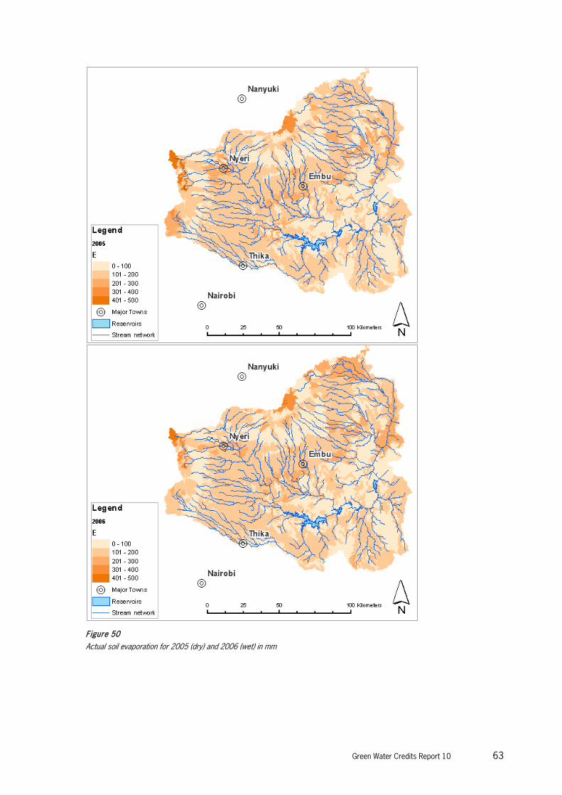
Green Water Credits Report 10 63
Figure 50
Actual soil evaporation for 2005 (dry) and 2006 (wet) in mm

64 Green Water Credits Report 10
Figure 51
Percentage of total actual evapotranspiration for 2005 (dry) and 2006 (wet)

Green Water Credits Report 10 65
Figure 52
Blue water (water entering water bodies by surface runoff and baseflow) for 2005 (dry) and 2006 (wet) in mm.

66 Green Water Credits Report 10
Figure 53
Deep groundwater recharge for 2005 (dry) and 2006 (wet) in mm
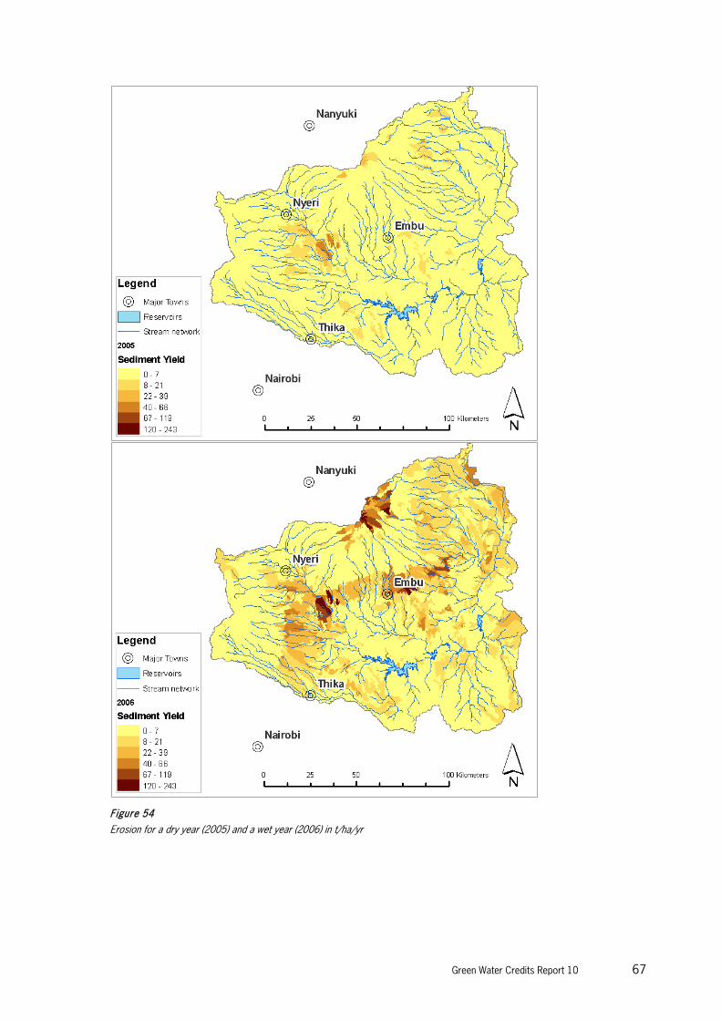
Green Water Credits Report 10 67
Figure 54
Erosion for a dry year (2005) and a wet year (2006) in t/ha/yr

68 Green Water Credits Report 10

Green Water Credits Report 10 69
4 Options for Green Water Credits
4.1 Potential benefits
Water is a finite resource, in other words, it cannot be created. However, the Proof-of-Concept phase of Green Water Credits showed that green water resources can be much increased and downstream delivery of blue water better regulated by increasing infiltration at the soil surface – minimising destructive runoff and “banking” this water in the soil – and by reducing unproductive evaporation. By arresting runoff, these practices conserve the soil, and increase groundwater recharge and thus stream baseflow. Soil and groundwater are natural reservoirs that hold orders of magnitude more water than all existing or conceivable man-made reservoirs. So Water Credits has potential benefits for both green water as well as blue water users: 1. Potential benefits for upstream land users:
a. More productive rainfed cropping, so higher crop water productivity and less non-productive evaporation from soil surface
b. Better water infiltration and retention in soil c. Reduced loss of soil nutrients by soil erosion during high intensity rainfall events
2. Potential benefits for downstream water users a. Augmented supply of blue water to reservoirs b. Augmented groundwater infiltration upstream to reduce peak flows (that in some cases cannot be
captured in the reservoirs) and to stimulate a more continuous supply/ better flow regime during the dry months
c. Reduced sediment input into reservoirs thus preserving capacity GWC is about meeting the objectives of both up- and downstream stakeholders at the same time. It is important to note that meeting the objectives separately would lead to other solutions; for example fertilizers, sediment traps, artificial groundwater recharge, etc. However, Green Water Credits aims at a sustainable mechanism to be implemented by stimulating the interaction between up- and downstream stakeholders and ensuring simultaneous benefits for both. Upstream land and water management practices determine the green and blue water and sediment flows both in the upstream as well as the downstream areas of the basin. In other words, downstream users are highly dependent for their supply on the management practices used in the upstream areas. This chapter assesses this interaction between land management practices and the blue water and sediment flows to the downstream reservoirs. This will lead to the identification of target areas where the implementation of Green Water Credits is most effective and will lead to significant gains for upstream farmers and downstream water uses - as for example hydropower. 4.2 Proposed green water management practices
The Proof-of-Concept of Green Water Credits showed that the following green water management practices have potential to benefit both upstream as well as downstream stakeholders: – Permanent vegetative contour strips – Mulching – Tied ridges
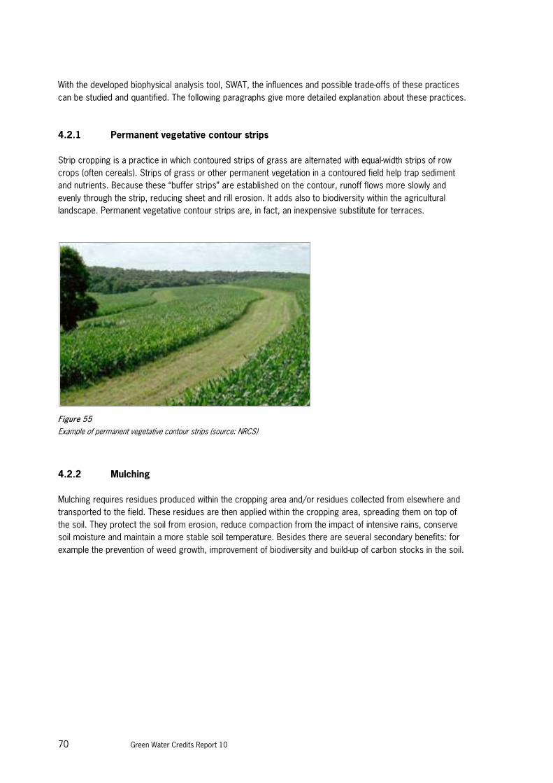
70 Green Water Credits Report 10
With the developed biophysical analysis tool, SWAT, the influences and possible trade-offs of these practices can be studied and quantified. The following paragraphs give more detailed explanation about these practices. 4.2.1 Permanent vegetative contour strips
Strip cropping is a practice in which contoured strips of grass are alternated with equal-width strips of row crops (often cereals). Strips of grass or other permanent vegetation in a contoured field help trap sediment and nutrients. Because these “buffer strips” are established on the contour, runoff flows more slowly and evenly through the strip, reducing sheet and rill erosion. It adds also to biodiversity within the agricultural landscape. Permanent vegetative contour strips are, in fact, an inexpensive substitute for terraces.
Figure 55
Example of permanent vegetative contour strips (source: NRCS)
4.2.2 Mulching
Mulching requires residues produced within the cropping area and/or residues collected from elsewhere and transported to the field. These residues are then applied within the cropping area, spreading them on top of the soil. They protect the soil from erosion, reduce compaction from the impact of intensive rains, conserve soil moisture and maintain a more stable soil temperature. Besides there are several secondary benefits: for example the prevention of weed growth, improvement of biodiversity and build-up of carbon stocks in the soil.
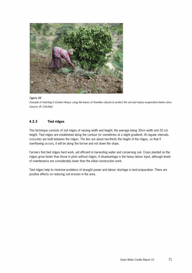
Green Water Credits Report 10 71
Figure 56
Example of mulching in Eastern Kenya: using the leaves of Grevillea robusta to protect the soil and reduce evaporation below citrus
(source: W. Critchley)
4.2.3 Tied ridges
This technique consists of soil ridges of varying width and height; the average being 30cm width and 20 cm height. Tied ridges are established along the contour (or sometimes at a slight gradient). At regular intervals, cross-ties are built between the ridges. The ties are about two-thirds the height of the ridges, so that if overflowing occurs, it will be along the furrow and not down the slope. Farmers find tied ridges hard work, yet efficient in harvesting water and conserving soil. Crops planted on the ridges grow faster than those in plots without ridges. A disadvantage is the heavy labour input, although levels of maintenance are considerably lower than the initial construction work. Tied ridges help to minimise problems of draught power and labour shortage in land preparation. There are positive effects on reducing soil erosion in the area.

72 Green Water Credits Report 10
Figure 57
Example of graded contour ridges with cross-ties lower than the main ridges to retain water between the ties, but allow excess
rainwater to flow along the furrows rather than spill over or break the main ridges (source: FAO)
4.3 Technical background
To assess how these practices affect the water and sediment flows in the basin, each of them was implemented in the model with the accompanying model parameter adjustments. The model parameters that represent these GWC options are the soil evaporation compensation coefficient (ESCO), the support practice factor for soil loss (Pusle) and the runoff curve number (CN2), each of them being described in the following paragraphs. 4.3.1 Soil evaporation
The soil evaporation compensation factor (ESCO) is a coefficient that has been incorporated to modify the depth distribution used to meet the soil evaporative demand. This factor accounts for the effect of capillary action, crusting and cracks, but also for other evaporation limiting or enhancing soil adjustments. ESCO must be between 0.01 and 1.0. As the value for ESCO is reduced, the model is able to extract more of the evaporative demand from lower levels of the soil (Figure 58). The default value for ESCO is 0.95. From the sensitivity analysis carried out during the Proof-of-Concept phase of Green Water Credits it was showed that ESCO can have a substantial impact on soil evaporation. Changing the default from 0.95 to 0.80 means an increase in soil evaporation of about 10%. On the other hand soil evaporation can be reduced by 10% when changing the coefficient from 0.95 to 0.99. Several studies have shown that besides the positive effect on erosion, mulching is able to reduce soil evaporation significantly, in some cases up to 40% (Chen et al. 2007; Tolk et al. 1999). These results have been used to define the parameter changes for the mulching scenario.

Green Water Credits Report 10 73
Figure 58
Impact of soil evaporation compensation factor ESCO on depth of evaporation extraction
4.3.2 Soil Erosion
Erosion and sediment yield were estimated for each HRU with the Modified Universal Soil Loss Equation (MUSLE) (Williams and Berndt 1977). While the USLE (Universal Soil Loss Equation) uses rainfall as an indicator of erosive energy, MUSLE uses the amount of runoff to simulate erosion and sediment yield.
PUSLE The support practice factor, PUSLE, is defined as the ratio of soil loss with a specific support practice to the corresponding loss with up-and-down slope cultivation. Support practices include contour tillage, strip cropping on the contour, and terrace systems. Stabilised waterways for the disposal of excess rainfall are a necessary part of each of these practices. Contour tillage and planting provides almost complete protection against
The modified universal soil loss equation is:
where sed is the sediment yield on a given day (metric tons), Qsurf is the surface runoff volume (mm H2O/ha), qpeak is the peak runoff rate (m3/s), areahru is the area of the HRU (ha), KUSLE is the USLE soil erodibility factor (0.013 metric ton m2 hr/(m3-metric ton cm)), CUSLE is the USLE cover and management factor, PUSLE is the USLE support practice factor, LSUSLE is the USLE topographic factor and CFRG is the coarse fragment factor. The crop management factor is recalculated every day that runoff occurs. It is a function of above-ground biomass, residue on the soil surface, and the minimum C factor for the plant.

74 Green Water Credits Report 10
erosion from storms of low to moderate intensity, but little or no protection against occasional severe storms that cause extensive break-through of contoured rows. The following tables from the scientific literature serve as guidelines for the definition of the scenarios and for future implementation of the management practices. Table 12 shows different values for PUSLE and slope-length limits for contour support practices. It is confirmed that contouring and the use of vegetative strips is most effective on slopes from 1 to 8 percent.
Table 12
P factor for different management practices, as studied in the United States (Wischmeier and Smith 1978)
Practice Slope Maximum length (m) P
Contour tillage 1 to 8% 122 to 61 0.5
9 to 12% 36 0.6
13 to 16% 24 0.7
17 to 20% 18 0.8
21 to 25% 15 0.9
Contour tillage between grass strips 1 to 8% 40 to 30 0.25 (r) 0.50
9 to 16% 24 0.30 (r) 0.60
17 to 25% 15 0.40 (r) 0.90
Table 13 shows the results of a study that was applied to the African situation. In this case mulching with straw led to a very high reduction in erosion.
Table 13
P factor for different management practices, as studied for West Africa (Roose 1977)
Management practice P
Tied contour ridging 0.2 to 0.1
Erosion control strips 2 to 4 m wide 0.3 to 0.1
Straw mulch, over 6 t/ha 0.01
Curasol mulch, 60 g/l/m² (depending on slope and crop) 0.5 to 0.2
Temporary pasture or cover plant (depending on cover) 0.5 to 0.01
Low earth bunds protected by stones or rows of perennial grass or low Dry stone walls every 80 cm +
contour tillage + hoeing + fertilization
0.1 to 0.05
The sensitivity analysis carried out during the Proof-of-Concept phase of Green Water Credits confirmed that PUSLE has a substantial impact on reducing soil erosion. In fact, there is a linear relationship between the coefficient and erosion rate (t/ha), as can also be seen from the previous soil loss equation. Those results and the boundary limits defined in the previous tables were used to define the scenarios for mulching and for the vegetative contour strips.
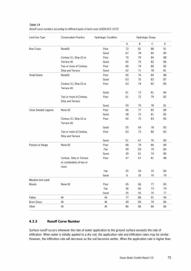
Green Water Credits Report 10 75
Table 14
Runoff curve numbers according to different types of land cover (USDA-SCS 1972)
Land Use Type Conservation Practice Hydrologic Condition Hydrologic Group
A B C D
Row Crops None(0) Poor 72 81 88 91
Good 67 78 85 89
Contour (1), Strip (2) or
Terrace (4)
Poor 70 79 84 88
Good 65 75 82 86
Two or more of Contour,
Strip and Terrace
Poor 66 74 80 82
Good 62 71 78 81
Small Grains None(0) Poor 65 76 84 88
Good 63 75 83 87
Contour (1), Strip (2) or
Terrace (4)
Poor 63 74 82 85
Good 61 73 81 84
Two or more of Contour,
Strip and Terrace
Poor 61 72 79 82
Good 59 70 78 81
Close Seeded Legume None (0) Poor 66 77 85 89
Good 58 72 81 85
Contour (1), Strip (2) or
Terrace (4)
Poor 64 75 83 85
Good 55 69 78 83
Two or more of Contour,
Strip and Terrace
Poor 63 73 80 83
Good 51 67 76 80
Pasture or Range None (0) Poor 68 79 86 89
Fair 49 69 79 84
Good 39 61 74 80
Contour, Strip or Terrace
or combination of two or
more
Poor 47 67 81 88
Fair 25 59 75 83
Good 6 35 70 79
Meadow (not used)
Woods
None (0) Poor 45 66 77 83
Fair 36 60 73 79
Good 25 55 70 77
Fallow All All 77 86 91 94
Brom Grass All All 49 69 79 84
Other All All 86 86 86 86
4.3.3 Runoff Curve Number
Surface runoff occurs whenever the rate of water application to the ground surface exceeds the rate of infiltration. When water is initially applied to a dry soil, the application rate and infiltration rates may be similar. However, the infiltration rate will decrease as the soil becomes wetter. When the application rate is higher than

76 Green Water Credits Report 10
the infiltration rate, surface depressions begin to fill. If the application rate continues to be higher than the infiltration rate once all surface depressions have filled, surface runoff will commence. In SWAT the SCS runoff equation is used (USDA-SCS 1972). This model was developed to provide a consistent basis for estimating the amounts of runoff under varying land use and soil types (Rallison and Miller 1981). The SCS curve number is a function of the soil’s permeability, land use and antecedent soil water conditions. Typical curve numbers for an average moisture condition (condition II) are listed in the following table for various land covers and soil types (USDA-SCS 1986). These values are appropriate for a 5% slope. The parameter changes for each of the scenarios were defined based on the sensitivity analysis performed during the Proof-of-Concept phase of Green Water Credits, and using the above table as the principal guideline. More details on the definition of the scenario parameters can be found in the following chapter. 4.4 Scenario definition
For each of the three proposed GWC management options (scenarios), the appropriate parameters were adjusted according to the following scheme. The SWAT model was used to evaluate these scenarios, and results were compared to the business-as-usual situation. It was assumed for these three management options that they would be implemented on the land uses shown in Table 15.
Table 15
Parameter changes for each of the scenarios
Management Practice Land use ESCO Pusle CN2
Baseline Scenario Baseline Scenario Baseline Scenario
Permanent Vegetative
Contour Strips
Maize
1.0
1.0
1.0
1.0
0.7 77 70
Coffee 0.7 77 65
Tea 0.7 77 65
Agric gen. 0.9 77 70
Mulching Maize 0.95
0.95
0.95
0.95
0.99 1.0
1.0
1.0
1.0
0.8
Coffee 0.99 0.8
Tea 0.99 0.8
Agric gen. 0.97 0.9
Tied ridges Maize 77 62
Agric gen. 77 62
The analysis is carried out by comparing the scenario output of a dry (2005) and a wet year (2006) with the reference “baseline” situation of the same year (Figure 36). The comparison is done using a number of indicators, graphics and maps, calculating the differences (absolute or percentage) between the baseline situation and scenario.

Green Water Credits Report 10 77
4.5 Scenario analysis
The three green water management practices as discussed in the previous section were implemented in SWAT, using the parameters as shown in Table 15. The dry and the wet years were selected for analysis and the differences in key indicators, water balance terms and spatial distribution were calculated and interpreted. The following sections discuss these results, separated in (1) key indicators, (2) crop-specific, and (3) the spatial distribution using maps. 4.5.1 Key indicators
In order to compare the three different green water management scenarios a set of indicators have been introduced showing the impact of each practice implemented basin-wide. Table 16 introduces these indicators with their values as obtained using the Upper Tana SWAT model for the baseline situation and the three different scenarios. Numbers reflect averages over the entire Upper Tana. The balance component “outflow” corresponds to the yearly total outflow at the proposed Low Grand Falls dam, the study basin outlet. The “Storage Change” state variable refers to the amount of water that flowed into (negative values) or out of (positive values) the basin storage compartments. Water is stored in the basin by the natural reservoirs (the aquifer and soil storage) together with the man-made reservoirs.
Table 16
Values of the key indicators for the baseline situation and the three scenarios
Key indicators 2005 2006 2005 2006 2005 2006 2005 2006Inflow Masinga (MCM/y) 860 2,144 857 1,999 879 2,171 852 2,012
Sediments Inflow Masinga (103ton/y) 1,219 4,130 908 3,165 1,227 4,142 892 3,247
Outflow Kiambere (MCM/y) 1,036 2,326 1,025 2,216 1,072 2,362 1,030 2,201
Outflow Low Grand Falls (MCM/y) 1,657 5,137 1,650 4,922 1,709 5,195 1,664 4,860
Crop Transpiration (mm/y) 382 360 383 360 387 363 383 361
Soil Evaporation (mm/y) 145 146 145 146 137 138 145 146
Groundwater Recharge (mm/y) 57 229 69 260 59 232 73 267
Sediment loss (ton/ha/y) 2 10 1 6 2 9 1 8
Precipitation (MCM/y) 9,099 18,759 9,099 18,759 9,099 18,759 9,099 18,759
Transpiration (MCM/y) -6,650 -6,264 -6,661 -6,271 -6,738 -6,316 -6,661 -6,273
Evaporation (MCM/y) -2,517 -2,533 -2,522 -2,540 -2,391 -2,399 -2,524 -2,542
Outflow (MCM/y) -1,657 -5,137 -1,650 -4,922 -1,709 -5,195 -1,664 -4,860
Storage Change (MCM/y) 1,725 -4,826 1,734 -5,025 1,739 -4,849 1,750 -5,083
Baseline data Tied RidgesContour Strips Mulching

78 Green Water Credits Report 10
For the baseline situation, inflows in Masinga range from 860 million cubic meters (MCM) in a dry year to 2144 MCM in a wet year. The maximum storage capacity of the Masinga reservoir is 1560 MCM, which means that during a wet year the entire water volume held in the reservoir is renewed. However, during a dry year, only about 60% of the maximum capacity of this first main reservoir (Masinga) enters as inflow. Sediment inflows into the Masinga reservoir are considerable. During the wet year 2006, the total sediment inflow was more than 4 million tonnes. This corresponds to about 2% of the total dead storage volume of the reservoir. Besides, the Upper Tana model calculated the total sediment inflow from 2001 until 2008 into this reservoir at about 16 million tonnes. This value corresponds to 9% of the original dead storage volume. This confirms that the sediment inflow into the reservoirs forms a serious threat to the water holding capacity. It is evident that significant gains can be obtained when the upstream sediment loss rates are reduced by implementing green water management practices. The impact of the green water practices on the key indicators can be seen from the same Table 16, but a more readily interpretable comparison (absolute and relative) is presented in Table 17 and in Figure 59. The table shows to what degree the key indicators changed for each of the scenarios compared to the baseline situation.
Table 17
Absolute and relative changes (green = increase, red = reduction) of the key indicators for the three scenarios compared to the
baseline situation
Key indicatorsInflow Masinga (MCM/y) -3 0% -145 -7% 19 2% 27 1% -8 -1% -132 -6%
Sediments Inflow Masinga (103ton/y) -311 -26% -965 -23% 8 1% 12 0% -327 -27% -883 -21%
Outflow Kiambere (MCM/y) -12 -1% -110 -5% 35 3% 36 2% -6 -1% -125 -5%
Outflow Low Grand Falls (MCM/y) -7 0% -215 -4% 52 3% 58 1% 7 0% -277 -5%
Crop Transpiration (mm/y) 1 0% 0 0% 5 1% 3 1% 1 0% 1 0%
Soil Evaporation (mm/y) 0 0% 0 0% -7 -5% -8 -5% 0 0% 1 0%
Groundwater Recharge (mm/y) 12 21% 31 14% 2 3% 3 1% 16 27% 38 17%
Sediment loss (ton/ha/y) -1 -45% -4 -39% 0 -12% -1 -13% -1 -32% -2 -21%
Precipitation (MCM/y) 0 0% 0 0% 0 0% 0 0% 0 0% 0 0%Transpiration (MCM/y) 11 0% 8 0% 88 1% 52 1% 11 0% 10 0%
Evaporation (MCM/y) 5 0% 7 0% -127 -5% -134 -5% 7 0% 9 0%
Outflow (MCM/y) -7 0% -215 -4% 52 3% 58 1% 7 0% -277 -5%Storage Change (MCM/y) 9 1% -200 -4% 14 -1% -24 0% 25 1% -258 -5%
2005 2006Tied Ridges
2005 2006 2005 2006MulchingContour Strips
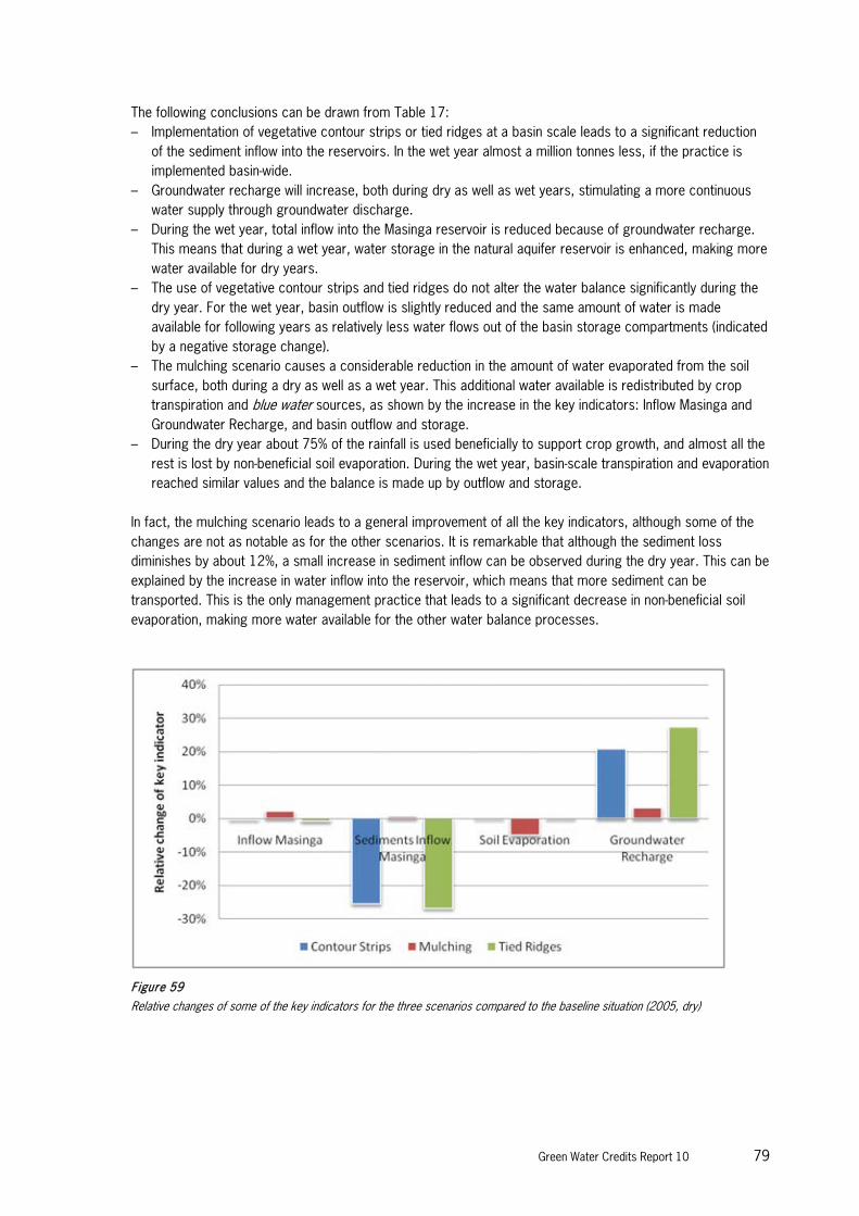
Green Water Credits Report 10 79
The following conclusions can be drawn from Table 17: – Implementation of vegetative contour strips or tied ridges at a basin scale leads to a significant reduction
of the sediment inflow into the reservoirs. In the wet year almost a million tonnes less, if the practice is implemented basin-wide.
– Groundwater recharge will increase, both during dry as well as wet years, stimulating a more continuous water supply through groundwater discharge.
– During the wet year, total inflow into the Masinga reservoir is reduced because of groundwater recharge. This means that during a wet year, water storage in the natural aquifer reservoir is enhanced, making more water available for dry years.
– The use of vegetative contour strips and tied ridges do not alter the water balance significantly during the dry year. For the wet year, basin outflow is slightly reduced and the same amount of water is made available for following years as relatively less water flows out of the basin storage compartments (indicated by a negative storage change).
– The mulching scenario causes a considerable reduction in the amount of water evaporated from the soil surface, both during a dry as well as a wet year. This additional water available is redistributed by crop transpiration and blue water sources, as shown by the increase in the key indicators: Inflow Masinga and Groundwater Recharge, and basin outflow and storage.
– During the dry year about 75% of the rainfall is used beneficially to support crop growth, and almost all the rest is lost by non-beneficial soil evaporation. During the wet year, basin-scale transpiration and evaporation reached similar values and the balance is made up by outflow and storage.
In fact, the mulching scenario leads to a general improvement of all the key indicators, although some of the changes are not as notable as for the other scenarios. It is remarkable that although the sediment loss diminishes by about 12%, a small increase in sediment inflow can be observed during the dry year. This can be explained by the increase in water inflow into the reservoir, which means that more sediment can be transported. This is the only management practice that leads to a significant decrease in non-beneficial soil evaporation, making more water available for the other water balance processes.
Figure 59
Relative changes of some of the key indicators for the three scenarios compared to the baseline situation (2005, dry)

80 Green Water Credits Report 10
It has to be noted that at a basin scale, the implementation of tied ridges gives very similar results to the scenario with vegetative contour strips. About the same reduction can be observed in sediment losses and reservoir inflow, and there is a similar basin-wide improvement in groundwater recharge. However, the tied ridges were only applied to the maize crops and the generic agricultural land use class, and not to the coffee and tea crops (Table 15). The spatial analysis (Section 4.5.3) shows other major differences between both practices. 4.5.2 Crop-based evaluation
The SWAT analysis tool allows a crop-specific assessment of the management practice’s impact on the crop water balance. The crop water balance of the baseline “business-as-usual” situation is shown in Figure 60. As can be seen, for the dry year surface runoff and groundwater recharge have a minor share in the water balance. Most of the water potentially available for the plants is used for crop growth through transpiration. On the other hand, during a wet year, about the same amount of water used for crop growth leaves the plots through surface runoff. Moreover, a considerable amount of water infiltrates and percolates to the aquifer.
Figure 60
“Business-as-usual” water balance of the three major cultivated crops for the two reference years
Maize Tea Coffee Maize Tea Coffee
Surface Runoff 42 54 45 294 247 240
Groundwater Recharge 39 30 53 203 167 239
Soil Evaporation 190 106 104 224 165 181
Crop Transpiration 201 468 438 205 375 333
0
200
400
600
800
1000
1200
Dept
h (m
m/y
)
2006 (wet)2005 (dry)

Green Water Credits Report 10 81
Figure 61
Changes of the crop water balances for the vegetative contour strips scenario compared to the baseline scenario
During the wet year (2006) much more water is lost by soil evaporation than during the dry year, due to the higher soil water content. Transpiration rates are similar, although slightly lower in the wet year due to differences in radiation and temperature. The crop water balances were compared with the baseline situation, and the absolute differences between the terms are represented in the following figures for each of the GWC management scenarios. Figure 61 shows that even during dry years, the use of vegetative contour strips causes a reduction in surface runoff (and erosion) and an increase in groundwater recharge. This additional water stored in the aquifer becomes then available for return flow or baseflow. This was confirmed by the basin water balance in Table 17, indicating that this management practice does not lead to a reduction in basin outflow or reservoir inflow during a dry year. The implementation of the mulching practice with the three main crops principally leads to changes in the evapotranspiration water balance (Figure 62). Productive crop transpiration is increased and soil evaporation is significantly reduced. This effect is similar both in the dry and in the wet year. Moreover, a slight increase in surface runoff and groundwater recharge can be observed, which means a minimal improvement in blue water availability.
Maize Tea Coffee Maize Tea Coffee
Surface Runoff -13 -24 -22 -64 -87 -98
Groundwater Recharge 12 24 22 49 60 72
Soil Evaporation 1 0 0 1 1 0
Crop Transpiration 1 2 0 1 1 0
-120
-80
-40
0
40
80
120
Dept
h (m
m/y
)
2006 (wet)2005 (dry)

82 Green Water Credits Report 10
Figure 62
Changes in the crop water balances for the mulching scenario compared to the baseline scenario
The implementation of tied ridges was only applied to the maize and the generic agricultural land use class. Figure 63 shows a significant reduction in surface runoff and a similar increase in groundwater recharge. The evapotranspiration terms are not affected by this practice.
Figure 63
Changes in the crop water balances for the tied ridges scenario compared to the baseline scenario
4.5.3 Spatial analysis
The Upper Tana catchment is heterogeneous in terms of climate, soil and topographical conditions. The effectiveness of the green water management practices depends on these site characteristics. Therefore, a spatial analysis and a comparison of the scenarios are necessary to provide knowledge about their spatial distribution and hydrological impact. This should give insight in where, and under which conditions, a certain practice contributes to the GWC objectives. This analysis is carried out on the scale of the finest modelling
Maize Tea Coffee Maize Tea Coffee
Surface Runoff 2 1 0 4 2 4
Groundwater Recharge 5 1 2 12 5 7
Soil Evaporation -24 -10 -11 -28 -11 -15
Crop Transpiration 16 10 11 12 4 6
-40
-30
-20
-10
0
10
20
30
40De
pth
(mm
/y)
2006 (wet)2005 (dry)
Maize Tea Coffee Maize Tea Coffee
Surface Runoff -23 0 0 -117 0 0
Groundwater Recharge 22 0 0 90 0 0
Soil Evaporation 1 0 0 1 0 0
Crop Transpiration 1 0 0 1 0 0
-150
-100
-50
0
50
100
150
Dept
h (m
m/y
)
2006 (wet)2005 (dry)

Green Water Credits Report 10 83
unit, the Hydrological Response Unit (HRU). Each of these units has a unique combination of climate conditions, soil, land use and topographical conditions. Erosion rates can be very high especially during years with high intensity rainfall events, resulting in high sediment inflow into the reservoirs. The yearly sediment loss can be up to four times higher than during a dry year (Table 16). Figure 64 shows the relative reduction obtained by the contour strips and tied ridges scenarios during the wet year. It has to be noted that the tied ridges scenario did not include any changes in the coffee and tea cultivated fields. As can be expected, the highest reductions are observed in the higher, steep slope areas, where the application of one of the practices leads to a reduction of about 50% in erosion. These are also areas where average rainfall intensity tends to be higher than in the lower part of the basin.
Figure 64
Spatial distribution of relative erosion reduction for the contour strips (left) and tied ridges (right) scenarios for the wet year
The yearly loss of water through soil evaporation is closely dependent on the meteorological conditions of that year. Figure 47 showed that during a dry and relatively hot year (2005) a relatively large part (about 25%) of the incoming precipitation is lost through soil evaporation, while during a wet year this loss represents a minor proportion of the total water balance. This means that it is of particular importance to reduce the soil evaporation during a dry year. The effectiveness of a certain practice, however, depends on the site conditions. Figure 65 shows that mulching reduces soil evaporation, but during the dry year this practice is more effective than during the wet year. Besides, this difference is accentuated in certain areas, as can be seen by comparing the spatial distribution of the simulated reduction.

84 Green Water Credits Report 10
Figure 65
Spatial distribution of relative reduction of soil evaporation for the mulching scenario for a dry year (left) and a wet year (right)
One of the main GWC objectives is to assure and enhance a more continuous flow regime during the year for better flood control and enhanced reservoir supply. Green water practices lead to less runoff and therefore to less instantaneous water supply to the reservoirs. Therefore, it is of crucial importance to verify that a reduction in runoff also leads to a comparable increase in groundwater recharge. This guarantees that the water becomes available through groundwater discharge, forming a more reliable and continuous water supply. Figure 66 shows both blue water competing variables: groundwater recharge (left) and runoff reduction (right) for the contour strips scenario. It is interesting to compare whether a reduction in runoff in a certain area is accompanied by a parallel increase in groundwater recharge. In fact, in the lower basin locations, a reduction of 10-25% in runoff comes with an increase of 25-50% in groundwater recharge. In the higher upstream areas, however, the percentages of relative change are similar between both variables. The following section makes use of these observations, by taking into account within one single classification different beneficial impacts of GWC practices, in order to identify potential target areas.
Figure 66
Spatial distribution of relative increase in groundwater recharge (left) and reduction of runoff (right) for the contour strips scenario
for a wet year

Green Water Credits Report 10 85
4.6 Results
4.6.1 Most effective practices
For the implementation phase of Green Water Credits it is crucial to decide, based on quantitative and socio-economical criteria, which of the practices have to be given priority. However, as we have seen in the spatial analysis, each of the practices has different impacts depending on the site characteristics. Using the spatial distribution of the impact on the different variables of groundwater recharge and erosion reduction, it is possible to compare the effectiveness of each of the practices. Applying this approach it will be possible to assess which of the practices has the most impact. Figure 67 (left) shows which of the practices leads to the highest increase in plant transpiration, location-specifically. In general, the mulching scenario gave the best results in most of the HRUs, both in the higher, wetter and cooler areas and in the drier areas. However, the use of vegetative contour strips in the higher regions can also lead to a comparable increase in transpiration. Thirdly, in a few regions applying tied ridges leads to a higher relative increase in transpiration than the use of mulch.
Figure 67
Spatial distribution of most effective practices with a positive impact on crop transpiration (left) and groundwater recharge (right)
for a dry year (2005)
Also, a comparison of the practices’ impact on groundwater recharge highlights the importance of a spatially distributed comparison. Figure 67 (right) shows which of the scenarios leads to the highest increase in groundwater recharge compared with the baseline situation. In general the application of tied ridges on the maize and non-specified agricultural fields is most effective in the majority of the HRUs. However, on a few sites mulching has a slightly higher positive impact on this indicator, although only during a dry year. Vegetative contour strips turn out to be more effective in the tea and coffee cultivated areas, both for the dry as well as for the wet year. The effectiveness of green water management measures depends on the yearly rainfall regime as shown in Figure 68. The left picture shows the spatial distribution of the most effective practices for reducing erosion, for a dry year (2005) and for a wet year (2006). One of the conclusions that can be drawn is that the more precipitation that falls, the more effective is the application of vegetative contour strips. Also the foregoing analysis showed that green water management practices are most effective and beneficial during wet years.

86 Green Water Credits Report 10
Accordingly, the identification of potential target areas for pilot operation was carried out using the impact assessment for the wet year 2006.
Figure 68
Spatial distribution of most effective erosion reduction practices for a dry year (left) and a wet year (right)
4.6.2 Potential target area identification
The scenario analysis was based on basin-wide implementation of management practices on all agricultural lands. One of the objectives of the current design phase of Green Water Credits is to define the potential target areas where the practices can be best implemented. The selection of target areas will depend on this hydrological and biophysical analysis, but also on socio-economic and institutional factors. This chapter makes an initial selection of potential sites based on the previously discussed scenario results for the biophysical aspects only. For the selection of target areas, the following indicators were chosen to represent overall impact of GWC: 1. Reduction in soil erosion 2. Increase in groundwater recharge 3. Increase in crop transpiration 4. Reduction in soil evaporation As discussed earlier, the impact of green water practices is greatest during wet periods. Erosion can be reduced significantly, groundwater recharge can be enhanced, storing more water in aquifers for drought periods - and the evapotranspiration can be optimised. If the most effective practice is chosen for implementation, Figure 69 shows the spatial distribution of the relative changes that can be obtained.

Green Water Credits Report 10 87
Figure 69
Spatial distribution of relative changes of four selected parameters for target area identification: (a) erosion reduction, (b)
groundwater recharge, (c) crop transpiration and (d) soil evaporation
The previous figures show clearly that the identification of target areas is a multi-criteria problem, as the spatial distribution of the maximum changes for each parameter is very different. Therefore, for the target area identification from a biophysical point of view, it is necessary to define weights to each of the parameters of interest. Given the objectives of Green Water Credits, it was decided to allocate equal importance to erosion reduction (weight = 0.5) as well as to the optimisation of green and blue water resources: groundwater recharge (0.25) and evapotranspiration (reduction in evaporation 0.125 and increased transpiration 0.125). The relative changes as shown in Figure 69 were rescaled to a value between 0 and 1, in which 0 means no benefit and 1 is the maximum benefit for the selected parameter. These 4 parameters were then used with the given weights within the following formula:
max)(125.0125.025.05.0
TAETGwRchSedYieldTA ⋅+⋅+⋅+⋅
=
The result of this scaled index TA used for target area identification is shown in Figure 70.

88 Green Water Credits Report 10
Figure 70
Spatial distribution of potential target areas
4.7 Conclusions
This biophysical assessment quantifies the benefits on the sediment and water flows resulting from green water management practices for the Upper Tana basin. It showed how much erosion and reservoir sediment input can be reduced, and the green water - blue water partitioning can be optimised through the implementation of the different management options. The key areas were also identified with the corresponding most effective practices. It is concluded that the implementation of vegetative contour strips or tied ridges within the most erodible parts of the basin could lead to a reduction in the sediment inflow to the Masinga reservoir of almost a million tonnes. The yearly sediment loss can be up to four times higher during a year with abundant precipitation than during a dry year. The highest erosion reductions are observed in the higher, steep slope areas, where the implementation of one of the practices is able to lead to a reduction of about 50%. Moreover, green water practices are more effective in these areas as they receive more rainfall than the lower parts of the basin. This assessment shows that there is an unambiguous benefit in optimising the use of the aquifer as a natural water storage facility within the basin. The reduction of runoff and the parallel enhancement of percolation and groundwater recharge reduce unproductive outflow from the reservoirs during intense rainfall periods as more water is retained upstream within the soil and aquifer. This stimulates a more continuous and reliable water supply during following dry periods. Green water management options are able to improve the usage of the

Green Water Credits Report 10 89
aquifer storage by about 20%. Moreover, it was confirmed that no significant reduction of reservoir inflow is caused during a dry year. The mulching scenario showed that a considerable reduction of water evaporated from the soil surface can be obtained, both during a dry and a wet year. This additional water is made available for crop transpiration (leading to a higher productivity) and blue water sources. The identification of potential target areas for pilot operation was done using the impact assessment of the wet year 2006, as in general the green water management practices are more effective during wet years (leading to less erosion and more benefits for optimal use of aquifer storage capacity). The selection of target areas was carried out based on the following parameters: soil erosion, groundwater recharge, crop transpiration and soil evaporation. The distributed approach used in this assessment allowed the spatial heterogeneity of the terrain to be accounted for. Therefore, the location of the target areas (Figure 70) depends on many factors including topography, soil type, etc. In general it can be concluded that the pilot operation of GWC is most relevant on the higher slopes of the Aberdares and Mount Kenya where coffee and maize is cultivated (average Target Area Index = 0.83 and 0.84 respectively). The use of a spatial index to summarise the benefits of each parameter of interest gives insight into the exact spatial distribution of the most appropriate areas. Results of these biophysical analyses will be combined with the socio-economic and institutional studies to determine the final selection of the pilot operation areas.

90 Green Water Credits Report 10

Green Water Credits Report 10 91
References
Asadullah A, McIntyre N and Kigobe M 2008. Evaluation of five satellite products for estimation of rainfall over Uganda. Hydrological Sciences Journal 53(6): 1137-1150
Batjes NH 2003. A taxotransfer rule based approach for filling gaps in measured soil data in primary SOTER databases. Report 2003/03, ISRIC - World Soil Information, Wageningen
Batjes NH and Gicheru P 2004. Soil data derived from SOTER for studies of carbon stocks and change in Kenya (ver. 1.0). Report 2004/01, ISRIC - World Soil Information, Wageningen
Chen SY, Zhang XY, PeD, Sun HY and Chen SL 2007. Effects of straw mulching on soil temperature, evaporation and yield of winter wheat: field experiments on the North China Plain. Annals of Applied Biology 150 (3): 261–268
Droogers P, Van Loon A, Immerzeel W 2008. Quantifying the impact of model inaccuracy in climate change impact assessment studies using an agro-hydrological model. Hydrology and Earth System Sciences 12: 1-10
Droogers P, Torabi M, Akbari M and Pazira E 2001. Field scale modeling to explore salinity problems in irrigated agriculture. Irrigation and Drainage 50: 77-90
Droogers P and Kite G 2001. Simulation modeling at different scales to evaluate the productivity of water. Physics and Chemistry of the Earth 26 (11-12): 877-880
FAO 2000. World-wide agroclimatic database, version 2.01, FAO, Rome Gatebe CK, Tyson PD, Annegarn HJ, Piketh S and Helas G 1999. A seasonal air transport climatology for
Kenya. Journal of Geophysical Research 104 (D12): 14,237 – 14,244 Jabro JD 1992. Estimation of saturated hydraulic conductivity of soils from particle distribution and bulk
density data. Transactions of the ASEA 35(2): 557-560 Jaetzold R and Schmidt H 1983. Farm management handbook of Kenya, Volume II - Natural conditions and
farm management information. Ministry of Agriculture, Nairobi KSS 1996. The Soil and Terrain Database for Kenya at scale 1:1,000,000 (ver. 1.0). Kenya Soil Survey,
National Agricultural Laboratory, Kenya Agricultural Research Institute KSS and ISRIC 2007. Kenya Soil and Terrain database - version 2. Kenya Soil Survey and ISRIC - World Soil
Information MWD 1992. The Study on the National Water Master Plan. Prepared with the assistance of Japan International
Cooperation Agency (JICA), Ministry of Water Development, Governement of Kenya Neitsch SL, Arnold JG, Kiniry JR, Williams JR and King KW 2002. Soil and Water Assessment Tool (SWAT).
Theoretical Documentation, version 2000, Taxes Water Resources Institute, College Station, Texas Rallison RE and Miller N 1981. Past, Present and Future SCS Runoff Procedure, International Symposium on
Rainfall-Runoff Modeling. Mississippi State University, Littleton pp 353-364 Roose E 1977. Application of the USLE in West Africa. In: Soil Conservation and Management in the Humid
Tropics. Greenland and Lal (eds.), John Wiley, pp 177-188 Shaxson F and Barber R 2003. Optimizing soil moisture for plant production: The significance of soil porosity,
FAO Soils Bulletin, Rome Sobieraj JA, Elsenbeer H and Vertessy RA 2001. Pedotransfer functions for estimating saturated hydraulic
conductivity: implications for modeling storm flow generation. Journal of Hydrology 251: 202-220 Sombroek WG, Braun HMH and van der Pouw BJA 1982. Exploratory soil map and agro-climatic zone map of
Kenya, 1980, scale 1:1,000,000. Exploratory Soil Survey report No E1, Kenya Soil Survey, Ministry of Agriculture, Nairobi
Tolk JA, Howell TA and Evett SR 1999. Effect of mulch, irrigation, and soil type on water use and yield of maize. Soil and Tillage Research 50 (2): 137-147

92 Green Water Credits Report 10
USDA-SCS 1972. National Engineering Handbook, Hydrology Section, Chap.4-10. US Dept. of Agriculture, Soil Conservation Service, Washington
USDA-SCS 1986. Urban hydrology for small watersheds, US Dept. of Agriculture, Soil Conservation Service, Washington, DC, USA
Van Engelen VWP and Wen TT 1995. Global and National Soil and Terrain Digital Database (SOTER). Procedures Manual. ISRIC - World Soil Information, Wageningen
Van Engelen VWP, Batjes NH, Dijkshoorn K, and Huting J 2005. Harmonized Global Soil Resources Database (Final Report). Report 2005/06, ISRIC – World Soil Information, Wageningen
Vieux BE, Cui Z and Gaur A 2004. Evaluation of a physics-based distributed hydrologic model for flood forecasting. Journal of Hydrology 298: 155– 177
Williams JR and Berndt HD 1977: Sediment yield prediction based on watershed hydrology. Trans. Am. Soc. Agric. Eng., 20: 1100-1104
Wilschut LI 2010. Land Use Map of the Upper Tana, Kenya: Based on Remote Sensing. Green Water Credits Report 9, ISRIC - World Soil Information, Wageningen
Wischmeier WH and Smith D 1978. Predicting rainfall erosion losses: a guide to conservation planning. USDA-ARS Agriculture Handbook N° 537, Washington DC: pp 58

Green Water Credits Report 10 93
Addendum I
SWAT using Improved Soil and Landuse Data
Authors J.E. Hunink P. Droogers
Client ISRIC
FutureWater Costerweg 1G
6702 AA Wageningen The Netherlands
+31 (0)317 460050
www.futurewater.n

94 Green Water Credits Report 10
Green Water Credits Report 10 95
Summary
This publication is an addendum to the full report5, and was found necessary as new information came available during recent months on land use and soils within the Upper Tana catchment. Therefore it was decided to re-design the model with this information and update the principal outcomes of the assessment, in order to have the most accurate information available for follow-up action.
5 Hunink et al. 2011. Impacts of Land Management Options in the Upper Tana, Kenya: Using the Soils and Water Assessment Tool
– SWAT. Green Water Credits Report 10, FutureWaters and ISRIC – World Soil Information, Wageningen.

96 Green Water Credits Report 10

Green Water Credits Report 10 97
5 Model revision
5.1 Introduction
The additional information that came available recently on land use and soil distribution in the Upper Tana required an update of the model and its results, especially for the identification of the target areas. This update was done in close collaboration with local staff of the Water Resources Management Authority (WRMA) from Kenya in order to incorporate their knowledge and understanding on the input data and relate it to the outcomes. This collaboration included a two-week stay by WRMA staff in the Netherlands. The updated datasets that have been included in the new model are: 1. Land use map based on field work and remote sensing techniques carried out by ISRIC (2009). 2. Soil map and property estimates derived from SOTER and WISE databases (ISRIC) and taxotransfer
procedure (2009-2010). These updated datasets required a new definition of the calculation units of the SWAT model: the hydrological response units (HRUs), as they are unique combinations of land use, soil and slope. In the following sections each of these datasets and the HRU definition procedure are described briefly. 5.2 Land use
The land use map used for the updated model is the result of fieldwork and satellite image classification performed by ISRIC staff in 2009. To produce the final land use map of the Tana, the technique Support Vector Machine (SVM) classification was used with Landsat images of 2000 (Figure 71). No multi-temporal analysis was performed.

98 Green Water Credits Report 10
Figure 71
The new land use map (ISRIC, 2009)
For the areas south of the Tana river which are not part of the Green Water Credits focal areas but form part of the Tana basin, information from the Africover dataset was merged with the updated dataset to guarantee complete land use coverage for the model. The WRMA-staff had a close look at the land use map and corrected a small number of polygons which were misclassified. The following changes have been carried out: 1. Changed class “Bare tea” to “Tea”. 2. Replaced class “Flowers” to “Pineapples”. 3. Changed the “Maize” polygons in the southern part of the map and near Chiokariga to Rangelands. 4. Removed “Rice” from other areas apart from the Mwea irrigation scheme. 5. Removed erroneous polygons “Water” and changed to rangeland. 6. Corrected Urban centres and placed correctly. After having carried out these changes, the resulting land use map was resampled to 250m to use as input for the HRU definition procedure.
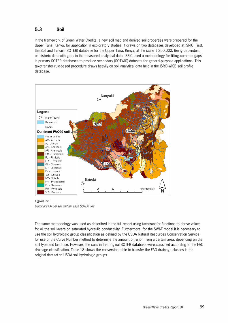
Green Water Credits Report 10 99
5.3 Soil
In the framework of Green Water Credits, a new soil map and derived soil properties were prepared for the Upper Tana, Kenya, for application in exploratory studies. It draws on two databases developed at ISRIC. First, the Soil and Terrain (SOTER) database for the Upper Tana, Kenya, at the scale 1:250,000. Being dependent on historic data with gaps in the measured analytical data, ISRIC used a methodology for filling common gaps in primary SOTER databases to produce secondary (SOTWIS) datasets for general-purpose applications. This taxotransfer rule-based procedure draws heavily on soil analytical data held in the ISRIC-WISE soil profile database.
Figure 72
Dominant FAO90 soil unit for each SOTER unit
The same methodology was used as described in the full report using taxotransfer functions to derive values for all the soil layers on saturated hydraulic conductivity. Furthermore, for the SWAT model it is necessary to use the soil hydrologic group classification as defined by the USDA Natural Resources Conservation Service for use of the Curve Number method to determine the amount of runoff from a certain area, depending on the soil type and land use. However, the soils in the original SOTER database were classified according to the FAO drainage classification. Table 18 shows the conversion table to transfer the FAO drainage classes in the original dataset to USDA soil hydrologic groups.

100 Green Water Credits Report 10
Table 18
Conversion table from FAO drainage classes to soil hydrologic groups (USDA)
FAO drainage class Description Soil hydrologic group (USDA)
E Excessively well drained A
I Imperfectly drained C
M Moderately well drained B
P Poorly drained D
S Somewhat excessively well drained A
V Very poorly drained D
W Well drained A
For each layer of each SOTER soil unit, the following properties were incorporated into the model for each soil layer (maximum of 5 layers, each 20 cm): a) Moist bulk density b) Available water capacity c) Saturated hydraulic conductivity d) Organic carbon content e) Clay content f) Silt content g) Sand content h) USLE K factor i) Soil hydrologic group Figure 73 and Figure 74 show, respectively, the bulk density and the available water capacity of the first 20 cm of each soil unit. Both variables determine to a high level the storage dynamics of the soil profiles. As can be seen, the spatial variability is high for both variables, especially between the higher slopes of the Mount Kenya and the Aberdares, and the lower, dryer regions.

Green Water Credits Report 10 101
Figure 73
Bulk density for the first 20 cm of each soil unit
Figure 74
Available water capacity of each soil unit
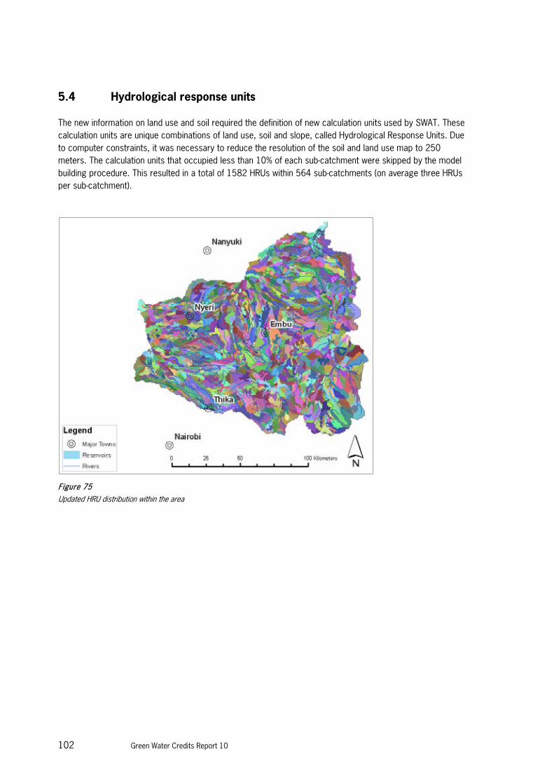
102 Green Water Credits Report 10
5.4 Hydrological response units
The new information on land use and soil required the definition of new calculation units used by SWAT. These calculation units are unique combinations of land use, soil and slope, called Hydrological Response Units. Due to computer constraints, it was necessary to reduce the resolution of the soil and land use map to 250 meters. The calculation units that occupied less than 10% of each sub-catchment were skipped by the model building procedure. This resulted in a total of 1582 HRUs within 564 sub-catchments (on average three HRUs per sub-catchment).
Figure 75
Updated HRU distribution within the area

Green Water Credits Report 10 103
6 Scenario analysis
The three green water management practices as discussed in the full report have been implemented in SWAT, using the same parameter changes. Instead of analysing the outcomes separately from a dry and a wet year, as was done in the full report, it was decided to do the analysis on 10-year averages. The following sections discuss the results of the (1) key indicators, (2) crop-based, (3) temporal analysis and (4) the target area identification. 6.1 Key indicators
In order to compare the three different soil and water management scenarios, a set of indicators were introduced as described in the full report. They show the impact of each of the basin-wide implemented practices. Table 16 lists the values for these indicators as obtained with the updated model for the baseline situation and the three management scenarios. Numbers reflect averages over the entire Upper Tana and over a 10-year period (2000-2009). The balance component “Outflow” corresponds to the yearly total outflow at the proposed Low Grand Falls dam, the study basin outlet. The “Storage Change” state variable refers to the amount of water that flowed into (negative values) or out of (positive values) the basin storage compartments (aquifers, soil storage and reservoirs).

104 Green Water Credits Report 10
Table 19
Values of the key indicators for the baseline situation and the three scenarios
On average, inflows into the Masinga reservoir are about 1500 MCM per year. The maximum storage capacity of the Masinga reservoir is of the same range, which means that on average the volume held in the reservoir is renewed every year. Sediment inflows into the Masinga reservoir are considerable. On average, yearly sediment inflow is more than 2 million tonnes. This corresponds to about 1% of the total dead storage volume of the reservoir. Besides, the Upper Tana model calculated the total sediment inflow from 2000 until 2009 into this reservoir at about 20 million tonnes. This value corresponds to more than 10% of the original dead storage volume. It has to be noted that these values are quite conservative compared to others found in the literature. This is because no calibration has been carried out on the sediment loads, as no data was available for this study. The relative impact of the green water management practices can be read from Table 16. This table shows to what degree the key indicators changed for each of the scenarios compared to the baseline situation.
Key indicators BaselineContour Strips Mulching
Tied Ridges
Inflow Masinga (MCM/y) 1,599 1,589 1,614 1,593
Sediments Inflow Masinga (103ton/y) 2,062 1,793 2,080 1,892
Outflow Low Grand Falls (MCM/y) 4,624 4,603 4,669 4,606
Crop Transpiration (mm/y) 364 364 367 364
Soil Evaporation (mm/y) 117 116 111 116
Groundwater Recharge (mm/y) 69 75 70 77
Sediment loss (ton/ha/y) 5 4 5 4
Basin Balance
Precipitation (MCM/y) 13,048 13,048 13,048 13,048
Transpiration (MCM/y) -6,328 -6,341 -6,377 -6,336
Evaporation (MCM/y) -2,027 -2,026 -1,924 -2,026
Outflow (MCM/y) -4,624 -4,603 -4,669 -4,606
Storage Change (MCM/y) -69 -78 -78 -80
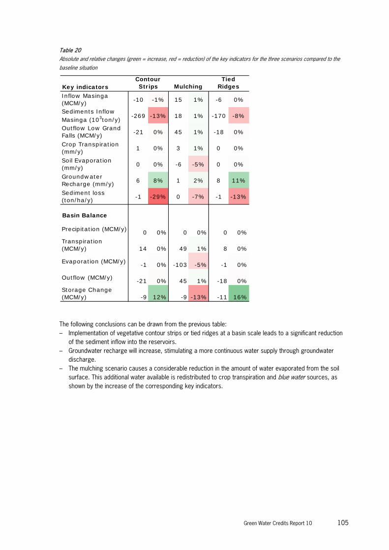
Green Water Credits Report 10 105
Table 20
Absolute and relative changes (green = increase, red = reduction) of the key indicators for the three scenarios compared to the
baseline situation
The following conclusions can be drawn from the previous table: – Implementation of vegetative contour strips or tied ridges at a basin scale leads to a significant reduction
of the sediment inflow into the reservoirs. – Groundwater recharge will increase, stimulating a more continuous water supply through groundwater
discharge. – The mulching scenario causes a considerable reduction in the amount of water evaporated from the soil
surface. This additional water available is redistributed to crop transpiration and blue water sources, as shown by the increase of the corresponding key indicators.
Key indicatorsInflow Masinga (MCM/y) -10 -1% 15 1% -6 0%
Sediments Inflow Masinga (103ton/y) -269 -13% 18 1% -170 -8%
Outflow Low Grand Falls (MCM/y) -21 0% 45 1% -18 0%
Crop Transpiration (mm/y) 1 0% 3 1% 0 0%
Soil Evaporation (mm/y) 0 0% -6 -5% 0 0%
Groundwater Recharge (mm/y) 6 8% 1 2% 8 11%
Sediment loss (ton/ha/y) -1 -29% 0 -7% -1 -13%
Basin Balance
Precipitation (MCM/y) 0 0% 0 0% 0 0%Transpiration (MCM/y) 14 0% 49 1% 8 0%
Evaporation (MCM/y) -1 0% -103 -5% -1 0%
Outflow (MCM/y) -21 0% 45 1% -18 0%Storage Change (MCM/y) -9 12% -9 -13% -11 16%
Contour Strips Mulching
Tied Ridges

106 Green Water Credits Report 10
Figure 76
Relative changes of three key indicators for the three scenarios compared to the baseline situation
6.2 Crop-based evaluation
The crop water balances were compared with the baseline situation, and the absolute differences between the terms are represented in the following figures for each of the GWC management scenarios. All calculations are based on yearly averages (2000-2009).
Figure 77
Absolute changes of the crop water balances for the vegetative contour strips scenario compared to the baseline scenario
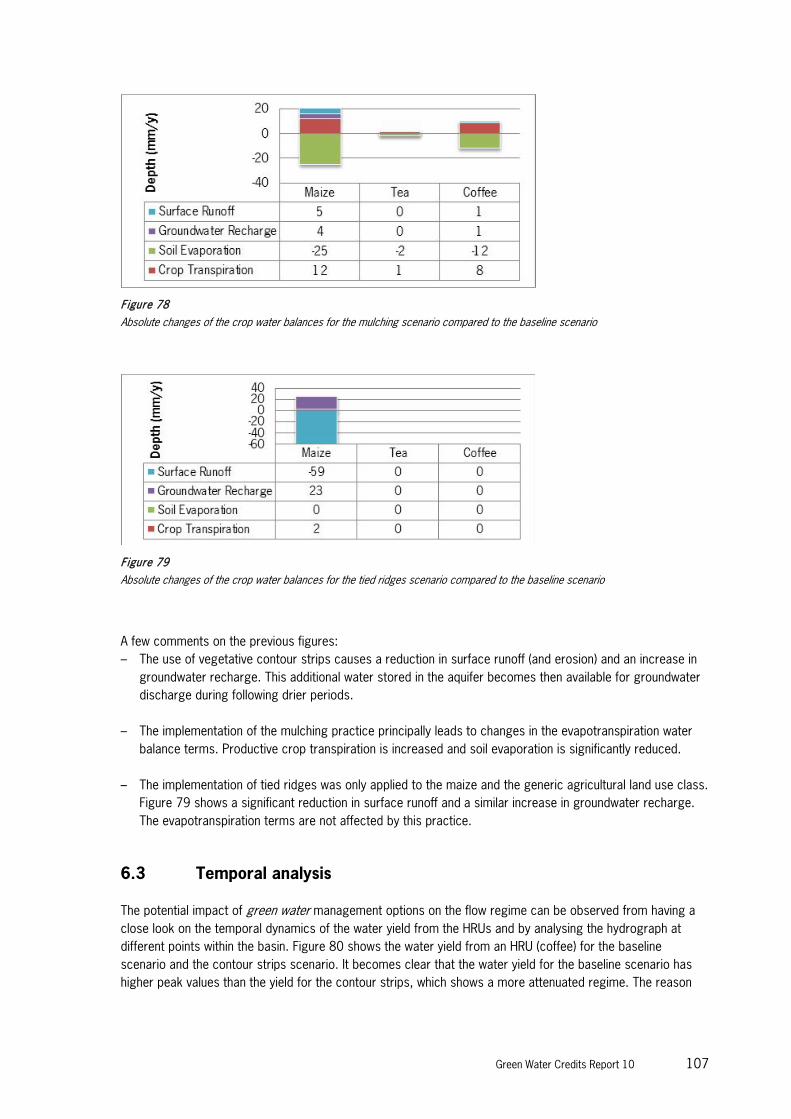
Green Water Credits Report 10 107
Figure 78
Absolute changes of the crop water balances for the mulching scenario compared to the baseline scenario
Figure 79
Absolute changes of the crop water balances for the tied ridges scenario compared to the baseline scenario
A few comments on the previous figures: – The use of vegetative contour strips causes a reduction in surface runoff (and erosion) and an increase in
groundwater recharge. This additional water stored in the aquifer becomes then available for groundwater discharge during following drier periods.
– The implementation of the mulching practice principally leads to changes in the evapotranspiration water
balance terms. Productive crop transpiration is increased and soil evaporation is significantly reduced. – The implementation of tied ridges was only applied to the maize and the generic agricultural land use class.
Figure 79 shows a significant reduction in surface runoff and a similar increase in groundwater recharge. The evapotranspiration terms are not affected by this practice.
6.3 Temporal analysis
The potential impact of green water management options on the flow regime can be observed from having a close look on the temporal dynamics of the water yield from the HRUs and by analysing the hydrograph at different points within the basin. Figure 80 shows the water yield from an HRU (coffee) for the baseline scenario and the contour strips scenario. It becomes clear that the water yield for the baseline scenario has higher peak values than the yield for the contour strips, which shows a more attenuated regime. The reason

108 Green Water Credits Report 10
for this is higher infiltration into the soil storage and percolation to the aquifer due to the use of vegetative contour strips. This results simultaneously in higher groundwater discharge a few days after the peak runoff. At that point, the full water yield originates from the groundwater discharge. For the contour strips scenario there is more streamflow in the river during days without rainfall compared to the baseline scenario.
Figure 80
Water yield and groundwater discharge for the baseline and contour strips scenarios
Another way to represent this positive impact of the GWC options is by plotting the absolute change in streamflow entering a reservoir (Masinga) under the contour strips scenario compared with the baseline scenario. Figure 81 shows the monthly precipitation amounts on the left axis and on the right, plotted in red, the difference in streamflow between scenarios. This graph shows that during a rainy month, less water enters the reservoir, while one or two months afterwards, higher inflow can be expected into the reservoir. The difference in the drier months can reach more than 10 m3/s. This means that about a million additional cubic meters of water a day enters into the reservoirs, which corresponds to three times the water demand of Nairobi city, and to about half of the current irrigation demand in the surrounding districts. This stresses the importance of green water management options for regulating flows and assuring a more continuous flow regime.

Green Water Credits Report 10 109
Figure 81
Precipitation compared to the change in reservoir inflow (Masinga) between baseline and contour strips scenario
6.4 Potential target area identification
The scenario analysis is based on basin-wide implementation of management practices on all agricultural lands. One of the objectives of the current design phase of Green Water Credits is to define the potential target areas where the practices are optimally implemented, from a biophysical point of view. As in the full report, for the selection of target areas the following indicators were chosen to assess the overall impact of GWC options: – Reduction in soil erosion – Increase in groundwater recharge – Increase in crop transpiration – Reduction of soil evaporation The absolute changes in these variables are shown in the following figures:

110 Green Water Credits Report 10
Figure 82
Spatial distribution of absolute changes that can be obtained of the four selected parameters for target area identification: (a)
erosion reduction, (b) groundwater recharge, (c) crop transpiration, and (d) soil evaporation
As was explained in the full report, the identification of target areas is a multi-criteria problem and requires an approach that integrates the four indicators into one single suitability index. In the full report, this index was based only on information from one single wet year (2006). In this case it was decided to use 10-year averages to calculate the biophysical suitability index (BSI), as defined in the following formula with the weights that correspond to each indicator:
max)(125.0125.025.05.0
BSIETGwRchSedYieldBSI ⋅+⋅+⋅+⋅
=
As can be observed in the formula, the index is scaled from 0 to 1, by dividing the weighted sum by the maximum value (BSI)max. This index was calculated for each of the HRUs, as shown in Figure 70. The highest

Green Water Credits Report 10 111
values for the Suitability Index can be seen on the eastern slopes of Mount Kenya and the slopes of the Aberdare mountain range (particularly the southern part of the Sagana sub-catchment).
Figure 83
Spatial distribution of potential target areas

112 Green Water Credits Report 10
Green Water Credits Report 10 113
7 Conclusions
The key indicators used to quantify the impact of the green water management options show very similar results for the updated model compared to the former one used in the full report. This means that the same conclusions can be drawn regarding the potential of the management options to meet the Green Water Credits objectives. Most of all, the results reconfirm that the erosion rates and sediment inflow into the reservoirs form a serious threat to the water holding capacity of the reservoirs. Another considerable benefit for downstream stakeholders is the more continuous streamflow into the reservoirs during months with low rainfall. This is a result of more groundwater discharge upstream and less peak runoff which also benefits the upstream users (less erosion, less loss of nutrients etc.). Important changes on the outcomes of the updated model can be observed when looking at the spatial distribution of the potential target areas. These changes are mainly due to the differences in the land use map, compared to the former map used (Africover). Besides, the updated soil properties also changed the impact outcomes of the green water management options, and thus the identification of potential target areas. The identification of potential target areas for pilot operation was done using the model outcomes on the changes of four key indicators: soil erosion, groundwater recharge, crop transpiration and soil evaporation. For this addendum, it was decided to use 10-year averages instead of a single wet year for the assessment. Results of this biophysical suitability assessment will be the input of the following studies on the socio-economic and institutional issues in the areas. This will lead to the final selection of the pilot operation areas.

114 Green Water Credits Report 10
Green Water Credits Report 10 115
Addendum II
Evaluation of different management options
Authors Johannes Hunink Peter Droogers Sjef Kauffman Godert van Lynden Commissioned by ISRIC-IFAD FutureWater Technical Note
FutureWater Costerweg 1G
6702 AA Wageningen The Netherlands
+31 (0)317 460050
www.futurewater.nl

116 Green Water Credits Report 10

Green Water Credits Report 10 117
8 Introduction
The second phase of Green Water Credits focuses on operational design and aims at a more detailed assessment of the Green Water Credits mechanism. For the biophysical assessment component of the second phase, two reports were published: 1. “Biophysical assessment using SWAT” (November 2009), consisting of an updated analysis following the
Proof-of-Concept phase. The analysis was based on recent input data and calibration data and the modelling assessment was carried out with much more detail compared to the Proof-of-Concept study.
2. An addendum to the previous report came out in June 2010, reporting the results based on new information that was available on land use and soils.
So far three GWC measures have been explored: (i) contour strips, (ii) mulching, and (iii) tied ridges. A detailed inventory by KSS resulted in a more extended list of options to be explored. The current technical note briefly summarises the outcomes of the scenario analysis that was based on this list. The scenarios studied are: – Bench terraces – Conservation tillage – Contour tillage – Fanya juu terraces – Grass strips – Microcatchments for planting fruit trees – Mulching – Rangelands – Ridging – Riverine protection – Trash lines In order to analyse the impact of the proposed set of green water management options, the following steps have been carried out: – Collection of information on the scenarios from the WOCAT database6, in order to summarise their effects
on the principal relevant processes. – The field scale observations from the WOCAT database on the impact of each scenario have been
converted to the relevant SWAT parameters, in order to allow a basin-wide assessment. – The latest model for the Upper Tana has been used to implement the parameter changes and run the
model for each of the scenarios. – Results have been summarised, expressed in the key indicators as in previous reports. – Maps of the erosion reduction and groundwater recharge increase have been produced for each of the
scenarios, to allow evaluation of the spatial variability of the effectiveness of each of the scenarios.
6 www.WOCAT.net

118 Green Water Credits Report 10

Green Water Credits Report 10 119
9 Green water management measures
9.1 Soil and Water Conservation measures from the WOCAT database
The WOCAT database contains information about all the green water management measures that have been studied in this assessment. Their technical characteristics and observations on the processes on field scale are included. This information is crucial in evaluating which processes are impacted and to which extent. The following table lists the code references of each of the measures in the WOCAT database.
Table 21
Studied green water management measures and their references in the WOCAT database
1 Bench terraces SYR01, ETH32, SWI02 2 Conservation tillage HUN1, KEN30, PHI44, UNK01, SPA01, CHN41, SWI06,
SWI07, RSA43 3 Contour tillage HUN2; SPA01; ETH43 4 Fanya juu terraces KEN05, ETH49 5 Grass strips RSA35 6 Microcatchments for planting fruit trees BRK10e, ETH45, SYR03 7 Mulching SPA03, SWI01, CHN40 8 Rangelands RSA42, SYR02 9 Ridging ETH38, ETH43, ETH47, ETH49 10 Riverine protection 11 Trash lines UGA04, TZA10, ETH01, ETH10
Based on the WOCAT database descriptions and information, a concise summary was made of each of the measures. This is found in the following paragraphs. 9.1.1 Bench terraces
This measure is an embankment constructed along the contour by the use of stone and soil as a construction material (WOCAT: ETH32). The technology is used in areas where there is insufficient stone and slopes are steep. Terrace banks are established by digging soil and using this to shape the embankment. The stone is used on the downslope side (the terrace “riser”) for reinforcing the structure. Vegetation is planted on the top of the embankment. The purpose is to reduce runoff, decrease slope length, increase infiltration rate and consequently to minimise soil erosion. The structure requires regular maintenance. Stone can be used, but given soil conditions in Upper Tana this might not be necessary always. In order to properly stabilise the structure, livestock should not be allowed to graze in the areas where the structures are placed. Checking for breaks after heavy storms is necessary.

120 Green Water Credits Report 10
In terms of biophysical processes this measure will have the following impacts: – reduction in soil loss by erosion – reduced overland flow 9.1.2 Conservation tillage
This green water management measure is a combination of various approaches ranging from (i) conservation tillage such as zero tillage and/or reducing excessive tillage operations (WOCAT: PHI44) to (ii) ripping of soil (WOCAT: KEN30). Conservation tillage is the practice of planting seeds through the stubble of last season’s crop, rather than ploughing and discing the field. The stubble protects topsoil against loss of soil to wind and rain and reduces agrochemical runoff to streams. By not ploughing, farmers also conserve soil moisture, which can reduce irrigation demands. In Kenya, conservation tillage generally requires minimum tillage for ripping the soil. Ripping is performed in one pass, to a depth of 10 cm, after harvest. Spacing between the rip lines is 30 cm in the case of wheat. Deep ripping (subsoiling) with the same implement is done, when necessary, to break a plough pan and reaches depths of up to 30 cm. An adaptation to the ordinary plough beam (the common mouldboard “Victory” plough) makes adjustment to different depths possible and turns it into a ripper for surface and deeper ripping. The aim of ripping is to increase water infiltration and reduce runoff. In contrast to conventional tillage, the soil is not inverted, thus leaving a certain amount of crop residue on the surface. As a result, the soil is less exposed and not so vulnerable to the impact of splash and sheet erosion, and water loss through soil evaporation and runoff. In addition, there are savings in terms of energy used for cultivation. In terms of biophysical processes this measure will have the following impacts: – reduction in erosion – reduced overland flow – potential water loss by weed transpiration (if no contra-actions are taken) 9.1.3 Contour Tillage
This green water management option is a combination of contour line ploughing (WOCAT: HUN2) and soil bunds with contour cultivation (WOCAT: ETH43). The basis of the technology is annual ploughing. The ploughing and all other cultivation is carried out parallel to the contour lines. This way, erosion can be significantly decreased. The contour cultivation aims at the reduction of the sheet and surface runoff. It is applicable anywhere below a certain slope angle. Special education and investment are not required, it can be realised with the available instruments. Soil bunds with contour cultivation can be applied on different land uses on slopes of more than 3%. Stone and stone-faced bund height depends on the availability of stones. On average the width is 1-1.2 m and the height is 0.6-0.7 m. Bunds reduce the velocity of runoff and soil erosion, retain water behind the bund and allow it to infiltrate. It further helps in ground water recharging. Planning is carried out by community/group and individual discussions. A consensus on layout, spacing, implementation modalities and management requirements is reached before implementation. In general this technology is applicable in areas where soil is moderately deep and stones are available.
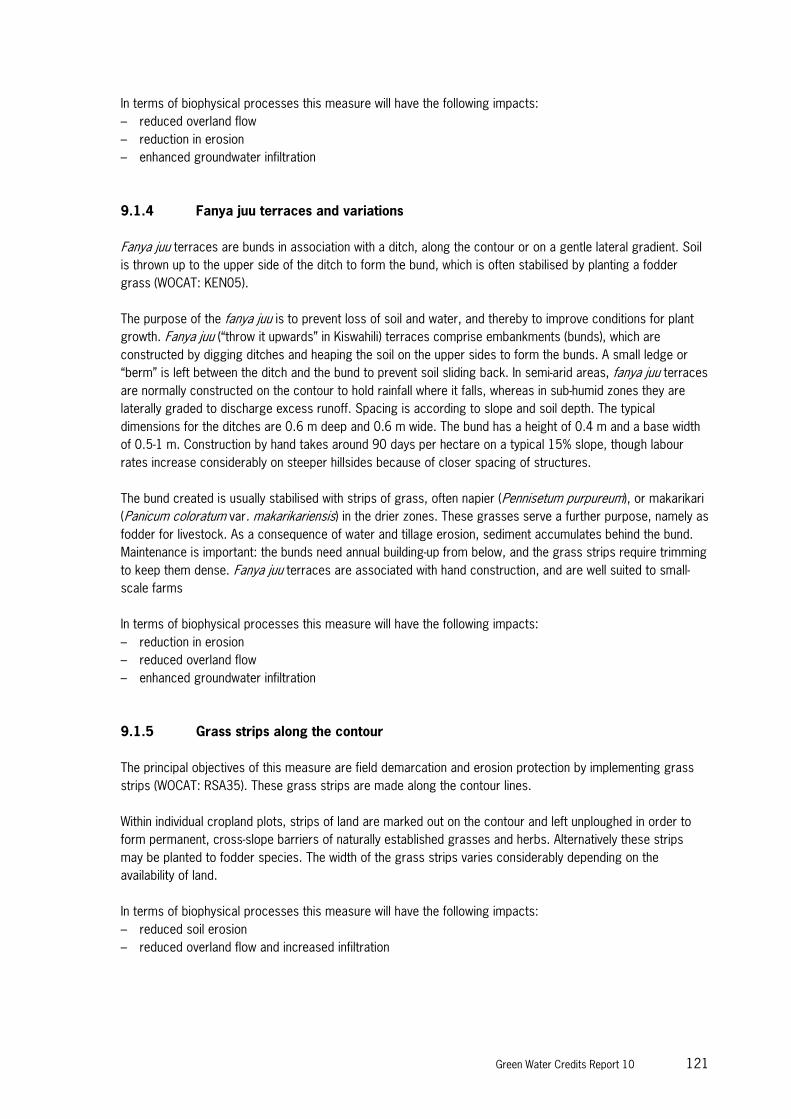
Green Water Credits Report 10 121
In terms of biophysical processes this measure will have the following impacts: – reduced overland flow – reduction in erosion – enhanced groundwater infiltration 9.1.4 Fanya juu terraces and variations
Fanya juu terraces are bunds in association with a ditch, along the contour or on a gentle lateral gradient. Soil is thrown up to the upper side of the ditch to form the bund, which is often stabilised by planting a fodder grass (WOCAT: KEN05). The purpose of the fanya juu is to prevent loss of soil and water, and thereby to improve conditions for plant growth. Fanya juu (“throw it upwards” in Kiswahili) terraces comprise embankments (bunds), which are constructed by digging ditches and heaping the soil on the upper sides to form the bunds. A small ledge or “berm” is left between the ditch and the bund to prevent soil sliding back. In semi-arid areas, fanya juu terraces are normally constructed on the contour to hold rainfall where it falls, whereas in sub-humid zones they are laterally graded to discharge excess runoff. Spacing is according to slope and soil depth. The typical dimensions for the ditches are 0.6 m deep and 0.6 m wide. The bund has a height of 0.4 m and a base width of 0.5-1 m. Construction by hand takes around 90 days per hectare on a typical 15% slope, though labour rates increase considerably on steeper hillsides because of closer spacing of structures. The bund created is usually stabilised with strips of grass, often napier (Pennisetum purpureum), or makarikari (Panicum coloratum var. makarikariensis) in the drier zones. These grasses serve a further purpose, namely as fodder for livestock. As a consequence of water and tillage erosion, sediment accumulates behind the bund. Maintenance is important: the bunds need annual building-up from below, and the grass strips require trimming to keep them dense. Fanya juu terraces are associated with hand construction, and are well suited to small-scale farms In terms of biophysical processes this measure will have the following impacts: – reduction in erosion – reduced overland flow – enhanced groundwater infiltration 9.1.5 Grass strips along the contour
The principal objectives of this measure are field demarcation and erosion protection by implementing grass strips (WOCAT: RSA35). These grass strips are made along the contour lines. Within individual cropland plots, strips of land are marked out on the contour and left unploughed in order to form permanent, cross-slope barriers of naturally established grasses and herbs. Alternatively these strips may be planted to fodder species. The width of the grass strips varies considerably depending on the availability of land. In terms of biophysical processes this measure will have the following impacts: – reduced soil erosion – reduced overland flow and increased infiltration

122 Green Water Credits Report 10
9.1.6 Microcatchments for planting fruit trees
Microcatchments for crop fields involve the construction of physical measures which trap rain water and help in increasing infiltration. Soil and stone bunds, micro-basins, ridges and tied ridges in various formations are some of the water harvesting techniques commonly referred to as microcatchments (WOCAT ETH45 and SYR03). All concentrate runoff for improved plant production. In the Upper Tana, these techniques are especially relevant in the context of planting fruit trees instead of coffee. Bunds can be established by digging channels and embanking the soil either on the upper side or on the downward direction. Often these are aligned in V-shapes to encourage concentration of water in the “V” for improved tree growth. Wherever stones are available they can be used to reinforce the ridges/bunds. Maintenance is crucial for proper implementation. This measure can be more considered as a change in land use rather than a classical soil and water conservation option. Microcatchments concentrate rain water at and around the cropped areas in order to enhance locally infiltration and increase production. Therefore, the following impacts in terms of biophysical processes can be expected:
• reduction of runoff if the structures are well maintained to increase infiltration locally 9.1.7 Mulching
Mulching requires residues produced within the cropping area and/or residues collected from elsewhere and transported to the cropping area. These residues are then applied in the field, spreading them on top of the soil. Mulching has been proven to protect the soil from erosion, reduce compaction from the impact of heavy rains, and tends to conserve soil moisture by reducing soil evaporation and maintain a more stable soil temperature. Furthermore there are several secondary benefits, as for example, inhibiting weed growth. The practice is thought to be economically beneficial in the long-term because of reducing fertility loss after heavy erosion events. In terms of biophysical impacts, the main processes affected are: – soil evaporation which can be reduced significantly – less soil erosion by protecting the soil 9.1.8 Rangelands
This scenario is a combination of measures to restore degraded rangelands using various approaches. The WOCAT database record RSA42 describes various options to restore degraded rangelands, each of them with different success and impacts, based on research done in South Africa. The treatments and measures that were positively evaluated (in terms of reduced erosion, increased soil water availability etc.) were used to assess this scenario in the Arid and Semi-Arid Lands (ASAL) around the main reservoirs. One measure that can be carried out in rangelands is the scooping out of small shallow “pits” in the ground, usually at the beginning or just before the rainy season (SYR02). Rainwater collects and soil moisture content is enhanced in and around the pits. Seeds which emerge in the pits find more favourable conditions for

Green Water Credits Report 10 123
emergence and growth. During the early growth stages, the young plants are also sheltered by the pits from wind. To assure optimum re-establishment of vegetation, grazing should be controlled during the initial establishment phase. The pits supply some additional water storage capacity to the fields, lowering runoff and enhancing infiltration. Reduced runoff may limit erosion; however, most of the erosion takes place during erratic heavy rainfall events in the semi-arid areas when no significant erosion reduction can be expected. 9.1.9 Ridging and tied ridges
This green water management option comprises either (i) an earth ridge formed by digging a furrow and piling the soil: a crop is planted on the ridge. The furrows may or may not be “tied” (WOCAT: ETH38); or (ii) soil bunds with contour cultivation (WOCAT: ETH43), stone faced embankments constructed along the contour to reduce soil loss (WOCAT: ETH 47). Farmers make the furrow and ridge by hand, and in some cases oxen scoops are used to move the soil and form the embankment. There are different methods employed in making ridges and furrows. The furrows are meant to collect rainwater. The plants benefit from the soil water stored in the furrows. Forming the ridges and basins is quite labour intensive. The ridges are frequently made anew each year, though in some cases the former ridges and furrows are maintained. The technology suit sub-humid and semi-arid agro-ecological zones with sandy to loamy soils. The main impacts of this measure in terms of biophysical processes are: – enhanced groundwater infiltration – increased capillary rise through increased water availability – reduced soil erosion 9.1.10 Riverine protection
Some farmers in the Upper Tana basin practice agriculture within the riparian reserve zone; that may eventually cause collapse of river banks and aggravate soil erosion. Cultivation within the seasonally dry riverbeds themselves also takes place in some areas. This causes disturbance of the river bed and the riverine zone. Protecting the banks along the rivers by planting of shrubs or trees (bamboo, fruit trees, etc.) could mitigate the impacts of these activities. Other Also possibilities are grass or other species (such as sugar cane) that cover the soil the whole year and may give returns to the local community in terms of cash or fodder for livestock. River bank erosion is thought to be an important process that especially occurs in the steep slope areas of the Aberdares and Mount Kenya. Protecting these banks with perennial plants could stabilise them and reduce direct sediment input into these water courses. The impact in terms of biophysical processes to be expected are: – Less sediment transported in the rivers – Less sedimentation of the reservoirs

124 Green Water Credits Report 10
9.1.11 Trash lines
Trash lines of organic material across the slope constitute a traditional land husbandry practice in some parts of Africa. Trash lines are usually composed of straw and weeds that are collected during primary cultivation (hand hoeing), and heaped in strips along the approximate contour. Trash lines are used in hillside fields where annual crops, including sorghum, finger millet, beans and peas are grown. They are a low-cost option for soil and water conservation. However, they need to be complemented by other measures on the steeper slopes. Trash lines reduce hillslope flow velocities and decrease the erosion rate and soil loss. Infiltration can be enhanced and soil may be trapped behind and within the trash lines themselves. The trash lines are not enough on their own to control erosion on the steeper slopes. In these areas they may reduce gully erosion when applied at the heads of the gullies to reduce flow velocities and gully incision. 9.2 Implementation in SWAT
The eleven GWC options as described before are included in the biophysical assessment tool (SWAT) to explore the impact on upstream as well as downstream soil and water flows and sediments. The following SWAT model parameters were considered to incorporate these GWC options: – Soil evaporation compensation coefficient (ESCO)
– higher value: reduced soil evaporation, more water available for transpiration or blue water – applicable at hru- or crop-level (file: hru)
– Support practice factor for soil loss (Pusle) – lower value: reduced erosion, increased recharge – applicable at hru- or crop-level (file: mgt)
– Runoff curve number (CN2) – lower value: reduced erosion, increased recharge – applicable at hru- or crop-level (file: mgt)
– Average slope steepness (SLOPE) – slope steepness different for each HRU, so adjusted by a factor. – lower value: reduced overland flow and erosion, increased recharge – applicable at hru- or crop-level (file: hru)
– Manning's "n" value for overland flow (OV_n) – higher value: more resistance to flow, lower flow velocities and erosion – applicable at hru- or crop-level (file: hru)
– Width of edge-of-field filter strip (FILTERW) – represents buffer zone around hru area – higher values: less erosion, more infiltration and less overland flow – applicable at hru- or crop-level (file: hru)
– Sediment deposition and re-entrainment (SPCON, SPEXP) – lower value: a lower sediment transport capacity of streams – applicable at basin level (file: bsn)
The following table summarises the parameter changes that were implemented in SWAT compared to the values of the baseline scenario (first row of the table). It should be emphasised that the assumption of these parameters is that implementation will take place on 20% of the fields. This assumption is also in line with the NRM-P project that focuses on 100,000 smallholders covering about 100,000 ha. Obviously if implementation was on larger areas, actual benefits could be expected to be higher.

Green Water Credits Report 10 125
Table 22
Parameter values and changes for each of the management scenarios
nr Scenario Land use ESCO PUSLE CN2 SLOPE OV_N FILTERW SPCON
0 Baseline All agricultural areas 0.95 1.0 77 100% 100% 0 0.001 1 Bench terraces Maize 0.8 75 95%
Coffee 0.8 70 95% Tea 0.9 70 95%
2 Conservation tillage Maize 0.96 0.9 200% 3 Contour tillage Maize 0.9 70 300% 4 Fanya juu terraces and
variations Maize 0.8 75 95% Coffee 0.9 70 95%
Tea 0.9 70 95% 5 Grass strips Maize 0.9 75 200%
Coffee 0.9 75 200% Tea 0.9 200%
6 Microcatchments for planting fruit trees
Maize 75 Coffee 75
Tea 75 7 Mulching Maize 0.99 0.8
Coffee 0.99 0.8 Tea 0.99 0.8
8 Rangelands Agricultural ASAL 0.96 0.8 200% Rangelands 0.96 0.8
9 Ridging Maize 62 10 Riverine protection All agricultural areas 0.0009 11 Trash lines Maize 0.96 75 2
Coffee 0.96 75 Tea 0.96

126 Green Water Credits Report 10

Green Water Credits Report 10 127
10 Results
The results presented in this chapter are based on the scenario implementation in SWAT. As in the previous reports, the key indicators and maps provide a basin-wide view and spatial insight in the impact of each of the scenarios on the key GWC-relevant processes. 10.1 Key indicators
The following key indicators are used to evaluate and quantify the impact of the GWC measures: – Annual water inflow into Masinga reservoir. – Annual sediment inflow into Masinga reservoir, determining its sedimentation rate. – Crop transpiration, determining crop production by upstream rainfed agriculture. – Soil evaporation, unproductive evaporation, including those of weeds. – Groundwater recharge, water that infiltrates into the soil and further percolates to the aquifer. – Erosion rate, soil lost by water erosion due to overland flow velocities. The impact of these indicators is best represented by assessing them for a dry year and wet year, to achieve quantitative insight into the range of the effectiveness of each of the scenarios. This approach also ensures that in the consequent analysis and implementation steps within the GWC scheme in the Upper Tana, the temporal variability is taken into account as a crucial factor, requiring long-term implementation and monitoring strategies. As in the previous assessment, the analysis was done for – a dry year (2005) with 523 mm of rainfall, and – a wet year (2006) with 1078 mm of rainfall. The key indicators are shown in Table 23, in which the changes are coloured according to their negative (red) or positive (green) relative increase or reduction compared to the baseline scenario. The first row shows the absolute values of the baseline scenario.

128 Green Water Credits Report 10
Table 23
Impact of the GWC measures on the key indicators
10.2 Maps
The following maps show the following relevant GWC processes, for each of the scenarios: – Groundwater recharge during a dry year (2005) – Erosion reduction during a wet year (2006) The first map shows the absolute values of the baseline scenario, and the eleven consecutive maps show the relative changes compared to the baseline scenario, expressed in its corresponding unit (t/ha/yr for erosion and mm/yr for groundwater recharge).
Inflow M
asinga
Sedim
ent inflo
w Mas
inga
Crop tr
ansp
iratio
n
Soil e
vaporatio
n
Groundwate
r rech
arge
Erosio
n
Scenario Land use* Year MCM/y Mton/y mm/y** mm/y** mm/y*** ton/ha/y*dry 931 1.0 335 121 16 1.2wet 2508 4.2 308 140 128 7.9dry 1.1% -21% 0% -1% 3% -23%wet 1.9% -21% 0% 0% 2% -18%dry 0.1% -1% 1% -5% 1% -2%wet 0.1% -1% 1% -4% 0% -1%dry 1.1% -10% 0% -1% 7% -12%wet 0.8% -7% 0% 0% 3% -6%dry 0.4% -21% 1% -1% 4% -23%wet 1.3% -20% 1% 0% 2% -18%dry 0.6% -11% 0% -1% 3% -14%wet 0.6% -10% 0% 0% 1% -10%dry 0.6% -8% 0% -1% 2% -8%wet 0.6% -6% 0% 0% 1% -5%dry 0.4% -6% 3% -12% 3% -9%wet 0.5% -6% 2% -12% 2% -8%dry 0.1% -4% 0% -3% 1% -4%wet 0.0% -2% 0% -2% 0% -6%dry 1.4% -18% 0% -1% 23% -21%wet 1.0% -12% 0% -1% 10% -12%dry 0.0% -5% 0% -1% 0% -5%wet 0.0% -4% 0% 0% 0% -4%dry 0.6% -7% 0% -3% 3% -8%wet 0.6% -6% 1% -2% 1% -5%
*M=Maize, C=Coffee, T=Tea,A=Agricul tura l ASAL, R=Rangelands ;
** Agricul tura l areas ; *** Bas in-wide;
11 Trash l ines
Baseline
1 Bench terraces
2 Conservation ti l lage
3 Contour ti l lage
4 Fanya Juu terraces and variations
5 Grass strips
6 Micro-catchments for planting fruit trees
7 Mulching
8 Rangelands
9 Ridging
10 Riverine protection
MCT
M
M
MCT
MCT
MCT
MCT
MCT
AR
M
MCTA
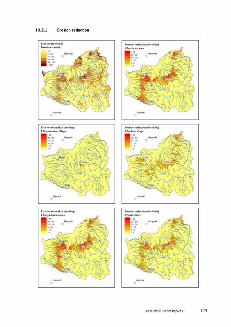
Green Water Credits Report 10 129
10.2.1 Erosion reduction

130 Green Water Credits Report 10
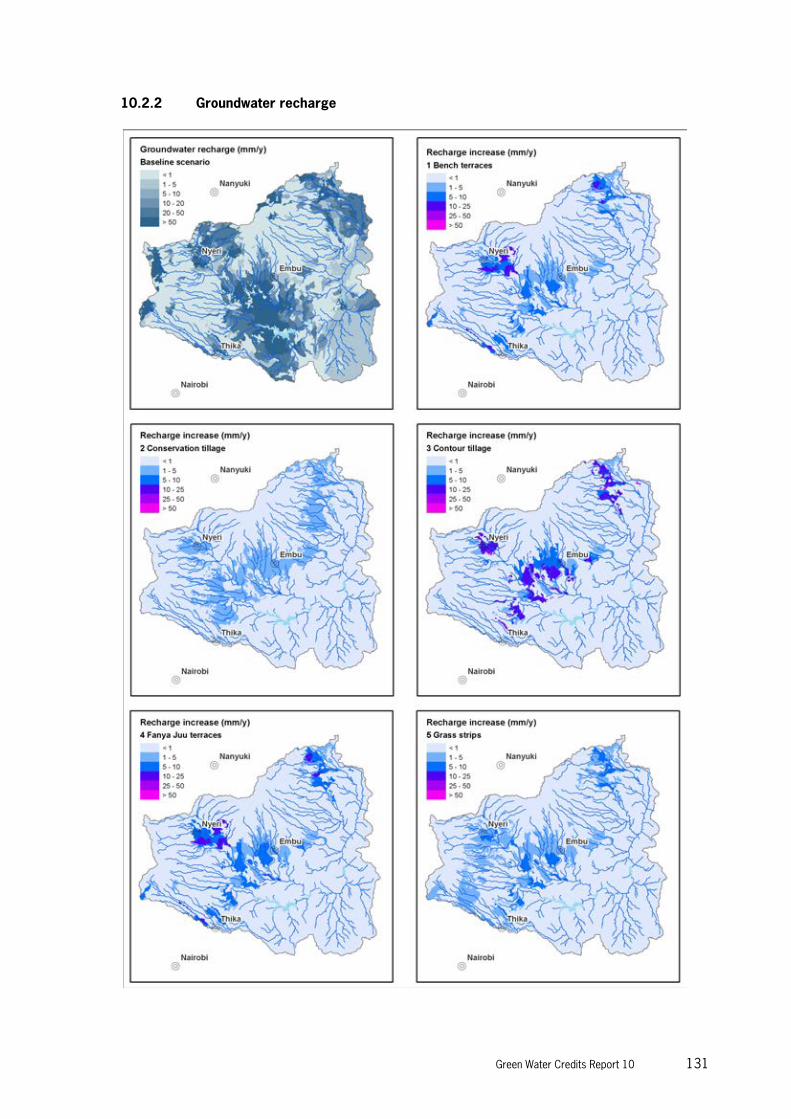
Green Water Credits Report 10 131
10.2.2 Groundwater recharge
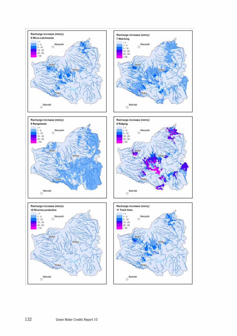
132 Green Water Credits Report 10

Green Water Credits Report 10 133
10.3 Main Conclusions
The concept of Green Water Credits addresses the sustainable management of the water resources in a river basin at source. It links the rain water that falls and is available to plants (green water) on rainfed land to the water (blue water) resources of rivers, lakes and groundwater. The importance of proper management of soil water to the provision of the blue water resources is often overlooked. One of the reasons for this is the difficulty in quantifying the potential impact of these measures. By using the SWAT model these potential benefits have been assessed for eleven measures. It was assumed that the eleven management measures explored during this study will be implemented on 20% of the area. This was considered as a realistic assumption and is similar to the NRM-P project that aims at about 100,000 smallholders. For transparency of the analysis, a mixture of measures was not considered, while in reality local-specific mixtures of measures will be implemented. The results presented here can be therefore considered as conservative. The most effective measures, in terms of getting reduced erosion, lower sedimentation of Masinga and higher water availability are the labour intensive structural measures (bench terraces, fanya juu and ridging). Results of these analyses will be used in two ways. First of all, the maps as presented in this chapter can be used to identify target areas. Second, results will be used in a benefit-cost analysis to explore downstream benefits and to express these benefit-costs in monetary values.

134 Green Water Credits Report 10

Green Water Credits Report 10 135
GWC Reports Kenya
GWC K1 Basin identification Droogers P and others 2006
GWC K2 Lessons learned from payments for environmental services Grieg Gran M and others 2006
GWC K3 Green and blue water resources and assessment of improved soil and water management scenarios using an integrated modelling framework.
Kauffman JH and others 2007
GWC K4 Quantifying water usage and demand in the Tana River basin: an analysis using the Water and Evaluation and Planning Tool (WEAP)
Hoff H and Noel S 2007
GWC K5 Farmers' adoption of soil and water conservation: the potential role of payments for watershed services
Porras IT and others 2007
GWC K6 Political, institutional and financial framework for Green Water Credits in Kenya
Meijerink GW and others 2007
GWC K7 The spark has jumped the gap. Green Water Credits proof of concept
Dent DDL and Kauffman JH 2007
GWC K8 Baseline Review of the Upper Tana, Kenya Geertsma R, Wilschut LI and Kauffman JH 2009
GWC K9 Land Use Map of the Upper Tana, Kenya: Based on Remote Sensing
Wilschut LI 2010
GWC K10 Impacts of Land Management Options in the Upper Tana, Kenya: Using the Soil and Water Assessment Tool - SWAT
Hunink JE, Immerzeel WW, Droogers P, Kauffman JH and van Lynden GWJ 2011
GWC K11 Soil and Terrain Database for the Upper Tana, Kenya
Dijkshoorn JA, Macharia PN, Huting JRM, Maingi PM and Njoroge CRK 2010
GWC K12 Inventory and Analysis of Existing Soil and Water Conservation Practices in the Upper Tana, Kenya
Muriuki JP and Macharia PN 2011
GWC K13 Estimating Changes in Soil Organic Carbon in the Upper Tana, Kenya
Batjes NH 2011
GWC K14 Costs and Benefits of Land Management Options in the Upper Tana, Kenya: Using the Water Evaluation And Planning system - WEAP
Droogers P, Hunink JE, Kauffman JH and van Lynden GWJ 2011
GWC K15 Cost-Benefit Analysis of Land Management Options in the Upper Tana, Kenya
Onduru DD and Muchena FN 2011
GWC K16 Institutes for Implementation of Green Water Credits in the Upper Tana, Kenya
Muchena FN and Onduru DD 2011
GWC K17 Analysis of Financial Mechanisms for Green Water Credits in the Upper Tana, Kenya
Muchena FN, Onduru DD and Kauffman JH 2011

136 Green Water Credits Report 10
ISRIC - World Soil Information
Ministry of Agriculture
Water Resources Management Authority
Kenya Agricultural Research Institute
Ministry of Water and Irrigation
International Fund for Agricultural Development
Future Water


ISRIC – World Soil Information has a mandate to serve the international community as custodian of global soil information and to increase awareness and understanding of soils in major global issues.
More information: www.isric.org
ISRIC – World soil Information has a strategic association with Wageningen UR (University & Research centre)
Green Water Credits Report 10
J.E. Hunink, W.W. Immerzeel, P. Droogers, J.H. Kauffman and G.W.J. van Lynden
Impacts of Land Management Options in the Upper Tana, Kenya Using the Soil and Water Assessment Tool - SWAT