Final Report

Moving to Goods and Services Tax in India: Impact on India’s Growth and International Trade

December 2009

Prepared for the Thirteenth Finance Commission Government of India

Project Team

Project Leader Rajesh Chadha

Research Team Anjali Tandon

Ashwani Geetha Mohan

Prabhu Prasad Mishra

Senior Consultant

M.R. Saluja

Consultants Devender Pratap

K. Elumalai

Computer Support Praveen Sachdeva

Library Support B.B. Chand

Secretarial Assistance Sudesh Bala

i

Foreword Tax policies play an important role on the economy through their impact on both efficiency and equity. A good tax system should keep in view issues of income distribution and, at the same time, also endeavour to generate tax revenues to support government expenditure on public services and infrastructure development. Cascading tax revenues have differential impacts on firms in the economy with relatively high burden on those not getting full offsets. This argument can be extended to international competitiveness of the adversely affected sectors of production in the economy. Such domestic and international factors lead to inefficient allocation of productive resources in the economy. This results in loss of income and welfare of the affected economy.

Value added tax was first introduced by Maurice Laure, a French economist, in 1954. The tax was designed such tha t the burden is borne by the final consumer. Since VAT can be applied on goods as well as services it has also been termed as goods and services tax (GST). During the last four decades VAT has become an important instrument of indirect taxation with 130 countries having adopted this, resulting in one-fifth of the world’s tax revenue. Tax reform in many of the developing countries has focused on moving to VAT. Most of these countries have gained thus indicating that other countries would gain from its adoption.

For a developing economy like India it is desirable to become more competitive and efficient in its resource usage. Apart from various other policy instruments, India must pursue taxation policies that would maximise its economic efficiency and minimise distortions and impediments to efficient allocation of resources, specialisation, capital formation and international trade. With regard to the issue of equity it is desirable to rely on horizontal equity rather than vertical equity. While vertical equity is based on high marginal rates of taxation, both in direct and indirect taxes, horizontal equity relies on simple and transparent broad-based taxes with low variance across the tax rates.

Traditionally India’s tax regime relied heavily on indirect taxes including customs and excise. Revenue from indirect taxes was the major source of tax revenue till tax reforms were undertaken during nineties. The major argument put forth for heavy reliance on indirect taxes was that the India’s majority of population was poor and thus widening base of direct taxes had inherent limitations. Another argument for reliance on indirect taxes was that agricultural income was not subjected to central income tax and there were administrative difficulties involved in collecting taxes.

The broad objectives of our study refer to analysing the impact of introducing comprehensive goods and services tax (GST) on economic growth and international trade; changes in rewards to the factors of production; and output, prices, capital, employment, efficiency and international trade at the sectoral level.

Analysis in this study indicates that implementation of a comprehensive GST in India is expected to lead to efficient allocation of factors of production thus leading to gains in GDP and exports. This would translate into enhanced economic welfare and returns to the factors of production, viz. land, labour and capital.

Suman Bery

Director General

ii

Acknowledgements

We would like to convey our sincere thanks to the Thirteenth Finance Commission, Government of India for having granted this important study to NCAER. Thanks are also due to the Directorate General of Foreign Trade, Ministry of Commerce and Industry, Government of India for part funding this work.

The NCAER research team has benefited immensely from very thoughtful inputs and suggestions received from Dr. Vijay Kelkar, Prof. Atul Sarma, Dr. Shashanka Bhide, Prof. Indira Rajaraman, Prof. M.R. Saluja and Shri B.K. Chaturvedi. We gratefully acknowledge their contributions and convey our sincere thanks to them.

We made three presentations of our work- in-progress at the Office of the Thirteenth Finance Commission on 8 October 2008, 12 June 2009 and 29 September 2009. The participants were actively engaged in debate and discussions during all the three sessions. As far as was possible, we have endeavoured to incorporate comments received by us. We would like to put on record our sincere thanks to all the participants, especially to Shri Sumit Bose, Shri Suman Bery, Prof. Subhashish Gangopadhyay, Dr. Rathin Roy, Shri Arbind Modi, Shri V. Bhaskar, Shri B.S. Bhullar, Prof. Mahesh C. Purohit, Prof. Kavita Rao, Prof. Basanta Pradhan, Dr. Anushree Sinha, Dr. Sanjib Pohit, Dr. Rajiv Kumar and Dr. R.N. Sharma.

iii

Table of Contents Executive Summary

I. Backdrop 1

II. India’s Tax Regime 2

III. Literature Survey 7

IV. Scheme of Analysis 11

V. Modelling GST 18

VI. Results 22

VII. Revenue Neutral GST Rate 27

VIII. Concluding Remarks 29

Tables 31

Bibliography 51

Annex-1 54

Annex-1 Tables 61

iv

List of Tables Table 1: Distribution of NIT across Sectors: Column-wise (Rs. Lakh) 31 Table 2: Percentage Change in Macro Variables 33 Table 3: Absolute Changes in Macro Variables over 2008-09 Values 34 Table 4: Percentage Change in Output 35 Table 5: Percentage Change in Output per Firm: Scale Effects 37 Table 6: Percentage Change in Employment 39 Table 7: Percentage Change in Capital 41 Table 8: Percentage Change in Export 43 Table 9: Percentage Change in Import 45 Table 10: Change in price index of tradable and non tradable goods (%) 47 Table 11: Distribution of NIT across Sectors: Row-wise (Rs. Lakh) 49

List of Figures Figure-1: Trend in Tax to GDP Ratio in India 4 Figure-2: Share of Indirect Tax in GDP for Year 2007 4 Figure-3: Share of Indirect Tax in Total Tax for Year 2007 4 Figure-4: Share of Net Indirect Tax in Output 15 Figure-5: Country-wise GST Rates 29

List of Boxes Box-1: Simulations Design 22 Box-2: Revenue Neutral GST Rates 28

Annex-1 Annex-1: Capital Coefficients Matrix 54 Box A: Distribution of Capital Formation by Type into IO Capital Good Sector (row-wise expansion of group output) 56 Box B: Distribution of Plant & Machinery Capital into IO Sectors (column-wise expansion of group output) 57 Table A1: Annual Survey of Industries 61 Table A2: Concordance between NIC 3-digit (2004) and IO 60 Sectors 62 Table A3: GFCF by type of assets at current prices (Rs. Crore) 65 Table A4: Mapping of the Non-Manufacturing Sectors with relevant IO sectors 70 Table A5: Price Indices used for Capital Formation 72 Table A6: Mapping between NIC and IO sectors for Output at constant prices 73 Table A7: Average Values of Capital Formation and Change in Output (Rs. Lakh) 74 Table A8: Capital Coefficient Matrix 77

v

Executive Summary

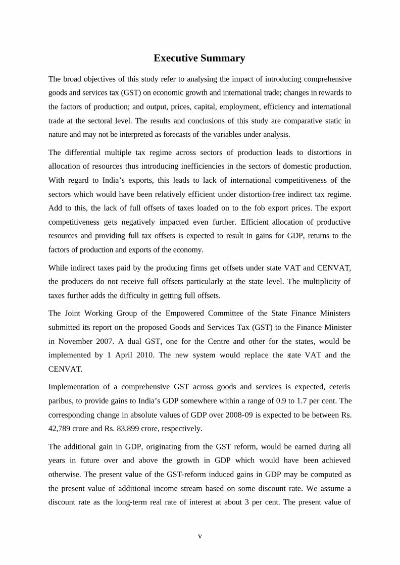
The broad objectives of this study refer to analysing the impact of introducing comprehensive

goods and services tax (GST) on economic growth and international trade; changes in rewards to

the factors of production; and output, prices, capital, employment, efficiency and international

trade at the sectoral level. The results and conclusions of this study are comparative static in

nature and may not be interpreted as forecasts of the variables under analysis.

The differential multiple tax regime across sectors of production leads to distortions in

allocation of resources thus introducing inefficiencies in the sectors of domestic production.

With regard to India’s exports, this leads to lack of international competitiveness of the

sectors which would have been relatively efficient under distortion-free indirect tax regime.

Add to this, the lack of full offsets of taxes loaded on to the fob export prices. The export

competitiveness gets negatively impacted even further. Efficient allocation of productive

resources and providing full tax offsets is expected to result in gains for GDP, returns to the

factors of production and exports of the economy.

While indirect taxes paid by the producing firms get offsets under state VAT and CENVAT,

the producers do not receive full offsets particularly at the state level. The multiplicity of

taxes further adds the difficulty in getting full offsets.

The Joint Working Group of the Empowered Committee of the State Finance Ministers

submitted its report on the proposed Goods and Services Tax (GST) to the Finance Minister

in November 2007. A dual GST, one for the Centre and other for the states, would be

implemented by 1 April 2010. The new system would replace the state VAT and the

CENVAT.

Implementation of a comprehensive GST across goods and services is expected, ceteris

paribus, to provide gains to India’s GDP somewhere within a range of 0.9 to 1.7 per cent. The

corresponding change in absolute values of GDP over 2008-09 is expected to be between Rs.

42,789 crore and Rs. 83,899 crore, respectively.

The additional gain in GDP, originating from the GST reform, would be earned during all

years in future over and above the growth in GDP which would have been achieved

otherwise. The present value of the GST-reform induced gains in GDP may be computed as

the present value of additional income stream based on some discount rate. We assume a

discount rate as the long-term real rate of interest at about 3 per cent. The present value of

vi

total gain in GDP has been computed as between Rs. 1,469 thousand crores and 2,881

thousand crores. The corresponding dollar values are $325 billion and $637 billion.

The sectors of manufacturing would benefit from economies of scale. Output of sectors

including textiles and readymade garments; minerals other than coal, petroleum, gas and iron

ore; organic heavy chemicals; industrial machinery for food and textiles; beverages; and

miscellaneous manufacturing is expected to increase. The sectors in which output is expected

to decline include natural gas and crude petroleum; iron ore; coal tar products; and non-

ferrous metal industries. There are minor gains and losses in output of other sectors.

Intersectoral movements of labour and capital would be in line with changes in output with

these factors of production moving into sectors with increased output and away from others.

Gains in exports are expected to vary between 3.2 and 6.3 per cent with corresponding

absolute value range as Rs. 24,669 crore and Rs. 48,661 crore. Imports are expected to gain

somewhere between 2.4 and 4.7 per cent with corresponding absolute values ranging between

Rs. 31,173 crore and Rs. 61,501 crore.

The sectors with relatively high proportional increase in exports include textiles and

readymade garments; beverages; industrial machinery for food and textiles; transport

equipment other than railway equipment; electrical and electronic machinery; and chemical

products: organic and inorganic. The moderate gainers are agricultural machinery; metal

products; other machinery; and railway transport equipment. Exports are expected to decline

in agricultural sectors; iron and steel; wood and wood products except furniture; and cement.

There are minor gains and losses in exports of other sectors.

The major import gaining sectors include leather and leather products; furniture and fixtures;

agricultural sectors; coal and lignite; agricultural machinery; industrial machinery; other

machinery; iron and steel; railway transport equipment; printing and publishing; and tobacco

products. The moderate gainers include metal products; non-ferrous metals; and transport

equipment other than railways. Imports are expected to decline in textiles and readymade

garments; minerals other than coal, crude petroleum, gas and iron ore; and beverages.

Prices of agricultural commodities and services are expected to rise. Most of the

manufactured goods would be available at relatively low prices especially textiles and

readymade garments. Consequently, the terms-of-trade move in favour of agriculture vis-à-

vis manufactured goods within a range of 1.8 to 3.8 per cent.

vii

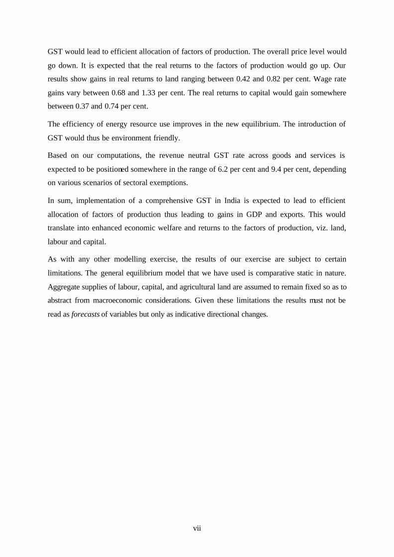
GST would lead to efficient allocation of factors of production. The overall price level would

go down. It is expected that the real returns to the factors of production would go up. Our

results show gains in real returns to land ranging between 0.42 and 0.82 per cent. Wage rate

gains vary between 0.68 and 1.33 per cent. The real returns to capital would gain somewhere

between 0.37 and 0.74 per cent.

The efficiency of energy resource use improves in the new equilibrium. The introduction of

GST would thus be environment friendly.

Based on our computations, the revenue neutral GST rate across goods and services is

expected to be positioned somewhere in the range of 6.2 per cent and 9.4 per cent, depending

on various scenarios of sectoral exemptions.

In sum, implementation of a comprehensive GST in India is expected to lead to efficient

allocation of factors of production thus leading to gains in GDP and exports. This would

translate into enhanced economic welfare and returns to the factors of production, viz. land,

labour and capital.

As with any other modelling exercise, the results of our exercise are subject to certain

limitations. The general equilibrium model that we have used is comparative static in nature.

Aggregate supplies of labour, capital, and agricultural land are assumed to remain fixed so as to

abstract from macroeconomic considerations. Given these limitations the results must not be

read as forecasts of variables but only as indicative directional changes.

1

Moving to Goods and Services Tax in India: Impact on India’s International Trade

I. Backdrop

India has posted high rates of growth since the early 1990s. It has become increasingly

integrated with the global economy. Exports have become an important engine of India’s

economic growth (Krueger, 2008). The share of exports (goods and services) in GDP has

increased from 8 per cent in 1990-91 to 14.7 per cent in 2000-01 and further up to 25.6 per

cent in 2008-09. Competitiveness of India’s exports has increased over time but gets partially

impeded due to certain domestic constraints. One of such constraining factors refers to

inefficient indirect tax regime.

Even though the country has moved on the path of tax reforms since the mid-1980s yet there

are various issues which need to be restructured so as to boost productivity and international

competitiveness of the Indian exporters. Sales of services to the consumers are not

appropriately taxed with many types of services escaping the tax net. Intermediate purchases of

inputs by the business firms do not get full offset and part of non-offset taxes may get added up

in prices quoted for exports thus making exporters less competitive in world markets (Poddar

and Ahmad, 2009). Even though we do not have precise numbers on the non-offset indirect tax

components for various sectors of production it may still be somewhere close to 20 to 30 per

cent of the total tax revenue.

The ongoing tax reforms on moving to a goods and services tax would impact the national

economy, international trade, firms and the consumers. A rich set of reports, papers and

books is available on issues relating to strengths and weaknesses of the India’s existing tax

regime. However, there has not been much work on the impact of tax reforms on India’s

international trade in a general equilibrium framework. The present study makes an attempt

to fill this gap albeit in a modest way. Analysis in this study is conducted using a computable

general equilibrium (CGE) model of the Indian economy (Chadha et al, 1998).

The broad objectives of our study refer to analysing the impact of introducing comprehensive

goods and services tax (GST) on economic growth and international trade; changes in rewards to

the factors of production; and output, prices, capital, employment, efficiency and international

trade at the sectoral level. The results and conclusions of this study are comparative static in

nature and may not be interpreted as forecasts of the variables under analysis.

2

II. India’s Tax Regime

Tax policies play an important role on the economy through their impact on both efficiency

and equity. A good tax system should keep in view issues of income distribution and, at the

same time, also endeavour to generate tax revenues to support government expenditure on

public services and infrastructure development. Cascading tax revenues have differential

impacts on firms in the economy with relatively high burden on those not getting full offsets.

This analysis can be extended to international competitiveness of the adversely affected

sectors of production in the economy. Such domestic and international factors lead to

inefficient allocation of productive resources in the economy. This results in loss of income

and welfare of the affected economy.

For a developing economy like India it is desirable to become more competitive and efficient

in its resource usage. Apart from various other policy instruments, India must pursue taxation

policies that would maximise its economic efficiency and minimise distortions and

impediments to efficient allocation of resources, specialisation, capital formation and

international trade. With regard to the issue of equity it is desirable to rely on horizontal

equity rather than vertical equity. While vertical equity is based on high marginal rates of

taxation, both in direct and indirect taxes, horizontal equity relies on simple and transparent

broad-based taxes with low variance across the tax rates.

Traditionally India’s tax regime relied heavily on indirect taxes including customs and excise.

Revenue from indirect taxes was the major source of tax revenue till tax reforms were

undertaken during nineties. The major argument put forth for heavy reliance on indirect taxes

was that the India’s majority of population was poor and thus widening base of direct taxes

had inherent limitations. Another argument for reliance on indirect taxes was that agricultural

income was not subjected to central income tax and there were administrative difficulties

involved in collecting taxes.

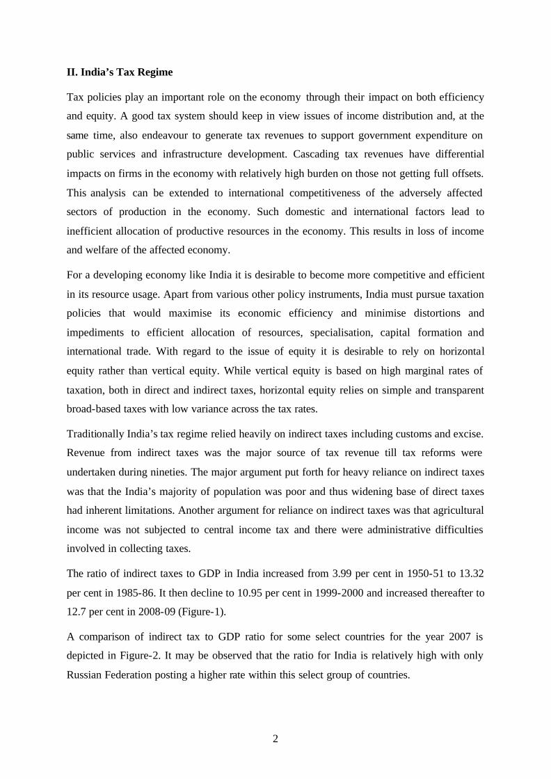
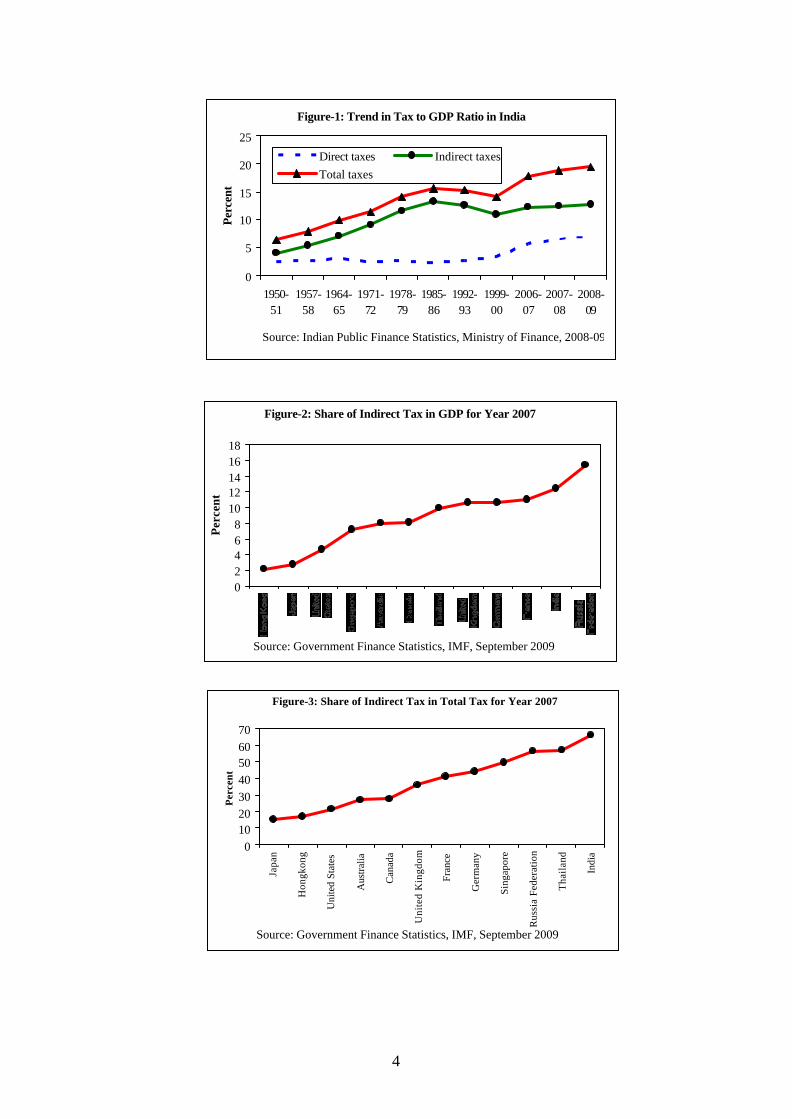
The ratio of indirect taxes to GDP in India increased from 3.99 per cent in 1950-51 to 13.32

per cent in 1985-86. It then decline to 10.95 per cent in 1999-2000 and increased thereafter to

12.7 per cent in 2008-09 (Figure-1).

A comparison of indirect tax to GDP ratio for some select countries for the year 2007 is

depicted in Figure-2. It may be observed that the ratio for India is relatively high with only

Russian Federation posting a higher rate within this select group of countries.

3

The share of indirect tax in total tax for the year 2007 is portrayed for the same select group

of countries in Figure-3. India has the highest share among this select group of countries.

In order to simplify and rationalise indirect tax structures, Government of India attempted

various tax policy reforms at different points of time. Through 1950s to 1970s, base of the

indirect taxes particularly excise duties was widened. In case of excise duty, attempts were

made to curb the consumption of luxury and semi luxury items, mopping excess profits in the

case of commodities in short supply and for encouraging exports. In 1975-76, a general levy

of one per cent ad valorem covering all goods produced for sale or other commercial

purposes not specified in the central excise tariff was imposed with exemptions for a few

items.

Around the same time, it became evident that indirect taxes lead to undesirable effects on

prices and allocation of resources. The Government of India constituted Indirect Taxation

Enquiry Committee in 1976 headed by Shri L. K. Jha to study the structure of indirect taxes,

central, state and local level taxes and suggest policy reforms. Indirect Taxation Enquiry

Committee submitted its report in 1978. The committee found a major problem with indirect

tax regime as it had caused unintended distortion in the allocation of resources and cascading

effects. The committee recommended that indirect taxation should move towards taxation of

final products and introduce modified form of value added tax.

However, a major obstacle in rationalisation of indirect tax system was the levy of tax on

commodities by government at different levels viz., centre, state and local authorities. This

multiple taxation provides incentives for tax evasion and undermines efficiency. Further,

there is lack of uniformity in the pattern of commodity taxation resulting in harassment to the

public by multiple tax authorities. Heavy reliance on indirect taxes for raising revenue was

also found to increase cost and fuel inflation.

The Government of introduced the Long Term Fiscal Policy (LTFP) on 19 December 1985

for prudent fiscal management. LTFP was expected to provide a definite direction and

coherence to annual budgets and to bring about a greater predictability and stability in the

economic system. It would provide rule based fiscal and financial policies rather than

discretionary approach. Further, it would also facilitate effective coordination of different

4

Figure-1: Trend in Tax to GDP Ratio in India

0

5

10

15

20

25

1950-51

1957-58

1964-65

1971-72

1978-79

1985-86

1992-93

1999-00

2006-07

2007-08

2008-09

Perc

ent

Direct taxes Indirect taxesTotal taxes

Source: Indian Public Finance Statistics, Ministry of Finance, 2008-09

Figure-2: Share of Indirect Tax in GDP for Year 2007

02468

1012141618

Per

cent

Source: Government Finance Statistics, IMF, September 2009

Figure-3: Share of Indirect Tax in Total Tax for Year 2007

010203040506070

Japa

n

Hon

gkon

g

Uni

ted

Stat

es

Aus

tralia

Can

ada

Uni

ted

Kin

gdom

Fran

ce

Ger

man

y

Sing

apor

e

Rus

sia

Fede

ratio

n

Tha

ilan

d

Indi

a

Per

cent

Source: Government Finance Statistics, IMF, September 2009

5

dimensions of economic policies. Major reforms in excise and customs taxation were

proposed under LTFP. These reforms were considered for progressively moving from

discretionary, quantitative restrictions and physical controls to non-discretionary fiscal

methods. The major reforms announced under Union excise taxation aimed at reducing the

number of effective rates after harmonisation of the tariff classification with the custom

nomenclature and implementing a modified system of value added taxation, i.e., MODVAT.

Excise duty is collected as CENVAT introduced in 2000 through re-naming of MODVAT of

1986.

However, fillip to tax policy reforms came in with the introduction of economic reforms in

1990s. It was realised that a complex tax structure involving both the centre and the states

taxing production and sales of commodities was not fostering efficiency in the economic

activities. The presence of central sales tax acted as constraint to inter-state trade movement

and contradicted the idea of India being a common market.

The Government of India constituted Tax Reforms Committee under the Chairmanship of Dr.

Raja J. Chelliah in August 1991 so as to bring comprehensive reforms in the Indian tax

system. The Committee suggested policy reform measures to restructure both direct and

indirect tax systems. For indirect tax, the Committee recommended reduction in the general

level of import tariffs comparable with similar developing countries, reduction in dispersion

of tariff rates and abolition of end use exemptions. The excise duty was to be progressively

converted from MODVAT to VAT. Some specific recommendations of the Tax Reforms

Committee included higher import tariffs on finished goods than basic raw materials and

moderate rates for components and machinery. Central excise duties were to be restructured

into three-rate MODVAT regime at the manufacturing level at 10, 15 and 20 per cent and

selective excise on nonessential commodities at 30, 40 and 50 per cent.

The 1990s tax reforms brought structural changes in the tax system. These reforms aimed at

correcting imbalances in the sources of revenues through increasing the share of direct taxes.

In July 2002, Government of India constituted a Task Force under the Chairmanship of Dr.

Vijay Kelkar to suggest measures for simplification and rationalisation of indirect taxes. The

Task Force recommended various measures including trust based customs clearance,

automation and modification of CENVAT rules to remove the distinction between capital

goods and inputs. On central excise, all duties should be replaced by only one levy, the

CENVAT. Scope of service tax should be expanded.

6

A system of VAT on services at the central government level was introduced in 2002. The

states collect taxes through state sales tax VAT, introduced in 2005, levied on intrastate trade

and the CST on interstate trade.

The Government of India constituted a Task Force on implementation of Fiscal

Responsibility and Budget Management Act, 2003 to chalk out a framework for fiscal

policies to achieve FRBM targets. Task Force headed by Dr. Vijay L. Kelkar made a number

of recommendations. Among others, it suggested an All India goods and services tax (GST)

which would help achieve a common market and widen the tax base. It recommended that the

multiplicity of tariffs should be reduced to three components viz., basic customs duty,

additional duty and anti-dumping duties. All exemptions should be removed barring life

saving drugs, security items, goods for relief and charitable purposes and international

obligations.

Despite all the various changes the overall taxation system continues to be complex and has

various exemptions. The Report of the Task Force on implementation of the FRBMA,

chaired by Dr. Vijay Kelkar, submitted its Report in July 2004. It has recommended

introduction of a national VAT on goods and services (GST) which would help improve the

revenue productivity of domestic indirect taxes and enhance welfare through efficient

resource allocation.

The Joint Working Group of the Empowered Committee of the State Finance Ministers

submitted its report on the proposed Goods and Services Tax (GST) to the Finance Minister

in November 2007. A dual GST, one for the Centre and other for the states, would be

implemented by 1 April 2010. The new system would replace the state VAT and the

CENVAT.

Most of the indirect taxes would be subsumed under GST except for stamp duty, toll tax,

passenger tax and road tax. All goods and services would be taxed with some exceptions.

There is a debate on the specific rate of the GST within a band varying from 12 to 20 per

cent. Nevertheless the move to GST would be one of the most important indirect tax reforms

in India.

An “Empowered Committee of the State Finance Ministers” (EC), constituted by the

Government of India in July 2000, submitted a White Paper on State-Level Value Added Tax

in January 2005. It suggested state VAT to have two basic rates of 4 per cent and 12.5 per

cent. There is an exempt category and a special rate of 1 per cent for a few selected items.

7

The items of basic necessities and goods of local importance are put under the exempted

category. Special rate of 1 per cent is applicable for Gold, silver and precious stones. The 4

per cent rate applies to other essential items and industrial inputs. The 12.5 per cent rate is

residual rate of VAT applicable to commodities not covered by other schedules. There is also

a category with 20 per cent floor rate of tax, but the commodities listed in this schedule will

not be subjected to VAT. This category covers items like motor spirit (petrol, diesel and

aviation turbine fuel), liquor, etc.

VAT system makes provision for eliminating the multiplicity of taxes. Several State taxes on

purchase or sale of goods have been subsumed in VAT. It also permits input tax credit. Since

VAT is implemented intra-state and does not cover inter-State sale transactions. Input credit

is not available for inter-state purchases. Further, exports will be zero-rated, and at the same

time, credit will be given for all taxes on inputs purchases related to such exports.

“A well designed destination-based GST on all goods and services is the most elegant method of

eliminating distortions and taxing consumption. Under this structure, all different stages of

production and distribution can be interpreted as mere tax pass-through, and the tax essentially

`sticks’ on final consumption within the taxing jurisdiction.” (Kelkar, 2009a).

“What would be the design of the GST? The broad framework of GST is now clear. This is on

the lines of the model approved by the Empowered Committee of the State Finance Ministers.

The GST would be a dual tax with both central and the State GST component levied on the same

base. Thus all goods and services barring a few exceptions will be brought into the GST base.

Importantly, there would be no distinction between goods and services for the purpose tax with a

common legislation applicable to both.” (Kelkar, 2009b).

III. Literature Survey

Value added tax was first introduced by Maurice Laure, a French economist, in 1954. The tax

was designed such that the burden is borne by the final consumer. Since VAT can be applied

on goods as well as services it has also been termed as goods and services tax (GST). During

the last four decades VAT has become an important instrument of indirect taxation with 130

countries having adopted this resulting in one-fifth of the world’s tax revenue. Tax reform in

many of the developing countries has focused on moving to VAT. Most of these countries have

8

gained thus indicating that other countries would gain from its adoption (Keen and Lockwood,

2007).1

McLure (2003) outlines characteristics of a well designed indirect tax regime in the context of

Canada. While consumers should be taxed at single rate sales of inputs to business should not

carry any tax liability. With regard to exports the tax should be levied under the destination

principle, i.e. exports should be tax-free and imports should be taxed at the same rate as

domestic products.

McLure points out some adverse outcomes emanating from inefficient indirect taxation:

• Differential tax regime on taxation of consumers on goods and services has adverse

implications for economic neutrality as well as equity. Consumers with relatively strong

preference for taxed goods are at disadvantage vis-à-vis consumers with the same

income level but preferring consumption of non-taxed / less taxed services. The equity

aspect refers to the fact that the higher income household allocate relatively proportion

of their incomes on purchase of services.

• Failure to provide full tax offsets to the business firms leads to distortions of choice of

methods of production based on the types of differentially taxed inputs and also impacts

household consumption patterns.

• Taxation of capital goods without apt offsets to business is perhaps the most serious

consequence of inefficient taxation system. This discourages savings and investment and

decelerates growth of productivity. 2

• Domestic producers face competitive disadvantage in the absence of destination based

taxation principle both between India and rest-of-world as well as across states.

• Some states may have more complex tax regime as compared with some other states.

Lack of proper coordination between the central and the state-level tax administration

creates complexities and cost inefficiency.

1 GST is VAT applied to goods and services. We would refer to GST though VAT may also be used as an alterative for the same. 2 “Perhaps the most celebrated example of tax-induced migration of industry is that of Intel, which built a new factory in New Mexico, rather than pay California sales tax on its construction costs. Although Intel is one of the quintessential corporations of the digital age, this episode could have occurred in any industry that was footloose.”, McLure (1998).

9

Imports which are currently implicitly subsidised (since much of these do not have to pay

intermediate taxes but only taxes at the final sale to the consumer) would be taxed under the

GST regime. While tariffs have protective effect, GST, through eliminating implicit subsidy

on imports, creates a level playing field. Thus GST does not distort domestic production.

Further, GST is superior to import tariffs since consumption provides a wider tax base than

imports so that tax on consumption has a smaller deadweight loss per rupee of revenue

collected (Bird and Gendron, 2007). Apart from improving export competitiveness, GST also

creates level playing field between imports and domestic production since it does away with

flawed structure of domestic indirect taxes.

One of the areas of interest has been to analyse the impact of moving to GST on resource

allocation and efficiency of sectors of production and on economy as a whole. Apart from

other analysis, Computable general equilibrium (CGE) models have also been used to assess

the impact of GST on an economy though there has not been much work on assessing the

impact of GST specific to international trade of an economy for all the sectors of an

economy.

Devarajan et al (1991) analyse the impact of introducing 10 per cent VAT in Thailand using a

general equilibrium model to identify gainers and losers and the effect on output, prices and

incomes. Though the paper provides an overall view of the changes in aggregate exports and

imports it does not bring out sectoral changes therein. It does not provide reference to the

type of the model used.

Wittwer and Kym (2002) use a computable general equilibrium model (CGE) to analyse the

impact of the GST and wine tax reform on Australia’s wine industry introduced in 2000. It is

concluded that export-oriented premium segment would gain at the expense of non-premium

segment of wine industry. The implicit message is that such gains would originate from

increased prospects of exports of the premium wine segment.

Meagher and Parmenter (1993) analyse short-run implications of Australia’s tax reforms of

1992 proposed as Fightback (Liberal and national Parties, 1992). Fightback was a radical

economic reform package and incorporated move to 15 per cent GST. They use a general

equilibrium model for their analysis. The conclusion states that: “The GST does not

discriminate between imports and domestic commodities and affects exports only in a minor

indirect way. Hence, its impact on cost-sensitive industries exposed to international

competition is smaller than the impacts of other taxes. Hence the implications of the GST for

10

output and employment are relatively small”. However, the paper does not lay out changes in

the composition of Australia’s foreign trade.

Dixon and Rimmer (1999) use a general equilibrium model to analyse the impact of

Australia’s tax reforms contained in Treasury Paper (ANTS) of 1998. ANTS programme

proposed tax reforms including move to 10 per cent GST. The paper concludes that the long-

run resource allocation gains flowing from the proposed tax changes will be negligible.

Terms-of-trade effect would be negative. Composition of exports would change away from

services and in favour of goods. For example, the package would harm tourism and benefit

traditional exporters like iron ore.

A desirable tax system should be able to enhance economy’s competitiveness through enabling

efficient allocation of productive resources thus resulting in increase in growth and increase in

real income of consumers in a country. Most of the static models focus on productive services of

primary factors of production. Such analysis does not incorporate the additional impact of

capital coefficients which, in turn, would enhance efficiency and result in higher returns to the

factors of production. Hamilton et al (1991) use a general equilibrium model to analyse the

impact of GST on economic growth in Canada. The federal sales tax (FST) in Canada, as in

1989, created several distortions. One of the important distortions refers to tax applied on capital

goods used in production process. It was about 4 per cent on capital goods. The removal of taxes

from capital goods would, over time, lower the cost of capital to domestic producers. This would

lead to increases in investments, productivity and domestic real output. The GST reforms would

have substantial impacts on real output, particularly for sectors which rely heavily on taxed

inputs and those which compete in the international markets – either exports or import-

competing domestic products. The GST reform would increase the real output of the Canadian

economy by approximately 1.4 per cent, i.e. about $9 billion over 1989.

GST is destination based. It implies export prices do not include any taxes while imports are

taxed at the same rates as domestically produced goods. It is generally believed that GST

encourages exports may be at the cost of imports or / and domestic consumption. But this may

not hold true according to the theory of international trade.3 The economic theory suggests that

the destination-based feature of GST does not affect exports and imports. Exchange rates adjust

to nullify the effects on imports and exports of moving to GST. However, the evidence from

136 countries in 2000 brings out contradiction between commonly believed view tha t GST

3 “In theory, the destination-based nature of a VAT should have no effect whatsoever on exports and imports. The reason is that exchange rates adjust to undo the effects of VATs on

11

encourages exports versus GST has no effect on trade pattern of a country. While the evidence

based on data for 1950-2000 showed negative relationship between GST and international trade

of a country a well-designed and properly-administered GST is expected to international trade of

countries adopting such reformed tax structure in future.

The evidence that the GST implementation by a country impedes international trade is based on

two undesirable reasons: a) GSTs were generally imposed heavily on traded sectors; and b)

governments often failed to provide adequate GST rebates for exports. However, there has not

been much work on empirical relationship between VAT usage and export and import

performance (Desai and Hines, 2002).

It is thus clear that it was lack of implementation of GST in letter and spirit that resulted in

distorted consequences. The GST must be applied on all sectors both tradable and non-tradable.

Thus all services must fall under the preview GST and that the export should be fully tax

rebated. The countries now introducing GST without weaknesses of the past would get benefits

of expansion of their international trade with special affect on exports.

While economic theory needs a careful review, there is case for implementing the GST in full

earnest. It should be applied across the board on all goods and services. Further the basic

purpose of analysing the effect of GST on international trade gets defeated if exporters do not

receive full tax offsets.

IV. Scheme of Analysis

4.1 Sources of Data

India’s international trade has increased rapidly during the last two decades. Differential

indirect tax rates in the economy without apt setoffs have lead to tax cascading which distort

production efficiency as well consumption pattern basket. Such taxes are likely to impact

comparative advantage of exports in sectors in which taxes paid on various inputs have not

been fully set off. This results in implicit taxation of such exports. Further, in the absence of

efficient input tax setoffs, productive resources would move towards less taxed sectors and

away from high taxed sectors.

We assume that the non-offset component of exports acts as export tax equivalent (ETE).

Once GST gets introduced, exporters would be able to take full credit of non-offset

components of the net indirect taxes (NIT) paid by them. This would make exports ‘zero-

rated’, i.e. subject to zero tax rates. GST would thus provide competitive advantage to India.

12

While much of the taxes paid on intermediate purchases by the business firms get rebates there

still exist components which do not get this benefit. While the Central indirect taxes including

customs and excise duties get nearly fully reimbursed, the state-level taxes do not get full

offsets. Some such state-level taxes include central sales tax (CST), electricity duty, sales tax on

petroleum products, mandi tax, entry taxes, octroi and municipal taxes. The cumulative impact

of such un-rebated taxes has been estimated as between 3 per cent to 12 per cent of the fob

export value depending on the product and its state of origin (Ministry of Commerce and

Industry, Government of India, 2009). These figures include 1 per cent to 9 per cent as

electricity duty, CST and sales tax on petroleum products and the remainder on account of

mandi tax, entry tax, octroi, municipal taxes and cesses (NCAER 2005). Since all taxes, central

as well as state, would be subsumed in GST exports are expected to become tax-free thus

enhancing competitiveness of Indian exporters. In fact, all local duties and cesses should also get

full offset through the instrument of GST.

The objective of this study is to estimate the impact of moving to a national GST, i.e. VAT

on both goods and services, on India’s foreign trade vis-à-vis the rest-of-world. It is expected

that non-rebated indirect tax-induced resource allocation distortions would be done away

with through state- level and centre- level GST and hence productivity of the economy would

increase thus leading to enhanced welfare. The changes in comparative advantage in different

sectors of production would alter composition of imports and exports – both of goods and

services.

The Input-Output Transactions Tables (IOTT) for 2003-04 along with data obtained from the

Annual Survey of Industries (2004-05) and the National Accounts Statistics (2008) provide

background information for our analysis.4 The base year thus predates the introduction of

state- level sales tax VAT though CENVAT was already in vogue. There are 130 sectors of

production – 37 primary, 68 manufacturing and 25 tertiary (discussion in the following

paragraphs of this section has been extracted from the background note on IOTT).

4 Input-Output Transactions Table - 2003-04, (2008): Central Statistical Organisation (CSO), Ministry of Statistics and Programme Implementation (MOSPI), Government of India. National Accounts Statistics (2008): Central Statistical Organisation (CSO), Ministry of Statistics and Programme Implementation (MOSPI), Government of India. Annual survey of Industries (2004-05): Central Statistical Organisation (CSO), Industrial Statistics Wing, Ministry of Statistics and Programme Implementation (MOSPI), Government of India.

13

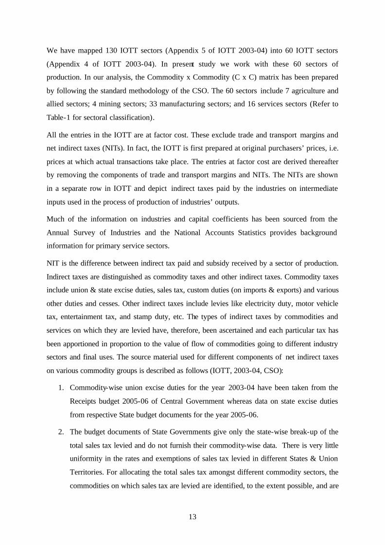
We have mapped 130 IOTT sectors (Appendix 5 of IOTT 2003-04) into 60 IOTT sectors

(Appendix 4 of IOTT 2003-04). In present study we work with these 60 sectors of

production. In our analysis, the Commodity x Commodity (C x C) matrix has been prepared

by following the standard methodology of the CSO. The 60 sectors include 7 agriculture and

allied sectors; 4 mining sectors; 33 manufacturing sectors; and 16 services sectors (Refer to

Table-1 for sectoral classification).

All the entries in the IOTT are at factor cost. These exclude trade and transport margins and

net indirect taxes (NITs). In fact, the IOTT is first prepared at original purchasers’ prices, i.e.

prices at which actual transactions take place. The entries at factor cost are derived thereafter

by removing the components of trade and transport margins and NITs. The NITs are shown

in a separate row in IOTT and depict indirect taxes paid by the industries on intermediate

inputs used in the process of production of industries’ outputs.

Much of the information on industries and capital coefficients has been sourced from the

Annual Survey of Industries and the National Accounts Statistics provides background

information for primary service sectors.

NIT is the difference between indirect tax paid and subsidy received by a sector of production.

Indirect taxes are distinguished as commodity taxes and other indirect taxes. Commodity taxes

include union & state excise duties, sales tax, custom duties (on imports & exports) and various

other duties and cesses. Other indirect taxes include levies like electricity duty, motor vehicle

tax, entertainment tax, and stamp duty, etc. The types of indirect taxes by commodities and

services on which they are levied have, therefore, been ascertained and each particular tax has

been apportioned in proportion to the value of flow of commodities going to different industry

sectors and final uses. The source material used for different components of net indirect taxes

on various commodity groups is described as follows (IOTT, 2003-04, CSO):

1. Commodity-wise union excise duties for the year 2003-04 have been taken from the

Receipts budget 2005-06 of Central Government whereas data on state excise duties

from respective State budget documents for the year 2005-06.

2. The budget documents of State Governments give only the state-wise break-up of the

total sales tax levied and do not furnish their commodity-wise data. There is very little

uniformity in the rates and exemptions of sales tax levied in different States & Union

Territories. For allocating the total sales tax amongst different commodity sectors, the

commodities on which sales tax are levied are identified, to the extent possible, and are

14

allocated to the respective sectors. The remaining amount of sales tax is allocated to the

different commodity sectors in proportion to the norms arrived on the basis of the

industry-wise data on sales tax from the ASI- 2003-04.

3. Imports are reported at c.i.f. values and are exclusive of import duties and domestic

taxes. The commodity-wise custom duties (both on imports and exports) are available

from the Ministry of Finance. Data on import duties have been used to build up

commodity sector-wise import duties (130 sectors). Adjustments have been made for

refunds & withdrawals to arrive at net import duties. Similarly, using the same

source, commodity-wise export duties/cesses have been prepared.

4. Source material used for “other indirect taxes” is the budget documents of state

governments and Finance Accounts of the Union and State Governments. These taxes

have been identified and allocated to the respective sectors of the IOTT.

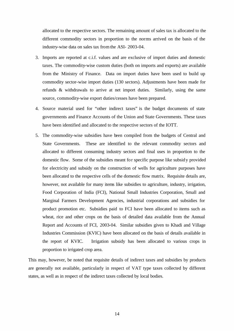
5. The commodity-wise subsidies have been compiled from the budgets of Central and

State Governments. These are identified to the relevant commodity sectors and

allocated to different consuming industry sectors and final uses in proportion to the

domestic flow. Some of the subsidies meant for specific purpose like subsidy provided

for electricity and subsidy on the construction of wells for agriculture purposes have

been allocated to the respective cells of the domestic flow matrix. Requisite details are,

however, not available for many items like subsidies to agriculture, industry, irrigation,

Food Corporation of India (FCI), National Small Industries Corporation, Small and

Marginal Farmers Development Agencies, industrial corporations and subsidies for

product promotion etc. Subsidies paid to FCI have been allocated to items such as

wheat, rice and other crops on the basis of detailed data available from the Annual

Report and Accounts of FCI, 2003-04. Similar subsidies given to Khadi and Village

Industries Commission (KVIC) have been allocated on the basis of details available in

the report of KVIC. Irrigation subsidy has been allocated to various crops in

proportion to irrigated crop area.

This may, however, be noted that requisite details of indirect taxes and subsidies by products

are generally not available, particularly in respect of VAT type taxes collected by different

states, as well as in respect of the indirect taxes collected by local bodies.

15

4.2 Indirect Tax - Matrix Structure

A matrix of net indirect taxes is available from CSO. It provides the aggregate value of

indirect taxes (130 x 130) paid during the IO transactions. Let NIT (i,j) denote net indirect tax

paid by sector-j for purchases of inputs from sector- i.

Summation NIT (i,j), i varying from 1-130, indicates the total of net indirect taxes paid by

sector-j for purchases of various inputs i (1-130) in its production process. This is the vertical

summation of all the net indirect taxes paid by the jth sector on purchases of various inputs

from 130 sectors.

Summation NIT (i,j), j varying from 1-130 is the sum of net indirect taxes paid by 130

sectors of production while buying inputs from sector- i. This thus indicates total net indirect

taxes paid on sales of sector-i to various sectors which purchase the output of sector- i as their

inputs. This is the horizontal summation of all the net indirect taxes paid by 130 sectors on

purchase of output of a particular sector as input in their respective production processes.

The ratios of total NIT to total output have large variations across sectors of production

(Table 1). The manufacturing sectors as a whole are subjected to 5.7 per cent NIT. The

corresponding ratio is 6.3 per cent in the case of capital goods and 5.3 per cent in buildings and

construction. 5 Thus net indirect tax rates are relatively high in capital goods as well as

construction vis-à-vis overall rate of 1.9 per cent for the economy as a whole. The overall NIT of

the seven capital goods sectors is higher than NIT of all the 33 manufacturing sectors taken

5 Capital goods sectors include Sectoral Classification Codes 37-43. Construction refers to Sector Code 45 (Table-1)

Figure-4: Share of Net Indirect Tax in Output

0.0

0.5

1.0

1.5

2.0

2.5

3.0

3.5

4.0

4.5

1968-69 1973-74 1978-79 1983-84 1989-90 1993-94 1998-99 2003-04

Per

cent

Source: CSO, Input-Output Transaction Table (2003-04)

16

together. Relatively high taxes on capital goods affect investment through higher cost of capital

(Bird et al).

The share of net indirect tax to output for India had increased from 2.9 per cent in 1968-69 to 4.1

per cent in 1978-79 and remained nearly the same till 1989-90 (Figure-4). It has declined

thereafter to 1.9 per cent in 2003-04.

4.3 Analytical Framework

The objective of this study is to analyse the impact of GST introduction on India’s foreign

trade. Net indirect taxes lead to distortions in domestic resource allocation. Sectors of

production which pay relatively high net indirect taxes without getting setoffs thereof might

lose out on allocation of new resources in favour of sectors which pay relatively low net

indirect taxes or receive full setoffs. Net indirect taxes may be viewed as implicit export tax

equivalents (ETE). In fact, exports of all the products which do not get tax offsets suffer

comparative disadvantage with high taxed sectors suffering relatively more vis-à-vis others.

The values of exports and imports during 2003-04 may be considered to be the base values.

The NCAER / Michigan stand-alone CGE model has been used for our analysis in this study.

The structural input coefficients, aij in the C x C matrix (Matrix-A) do not reflect capital

requirements of the economy. These represent flows from sector “i” to sector “j” of inputs

required to produce one rupee’s worth of output in the current year and are not representative of

the capital coefficients in each of the 60 sectors of the economy.

In the standard input-output flow matrix (IO), sector-wise inputs required for capital formation

are included in the final demand vector. In order to make the original input coefficients

representative of the capital requirements we formulate an additional matrix called the “Capital

Matrix - B”. The detailed methodology for computing of the B-matrix is presented in the

following discussion.

4.4 Leontief Dynamic Theory

Net indirect taxes on capital goods can have long-lasting effects on the economy if the same do

not get full offsets. This limits the growth of capital stock and reduce productivity and

employment over time (Smart and Bird, 2006).

The static input-output scheme used in earlier versions of our CGE model explains mutual

interdependence of some distinct sectors of the national economy in terms of a given set of

structural coefficients, aij (i = n; j = n). Each such coefficient represents the amount of the ith

17

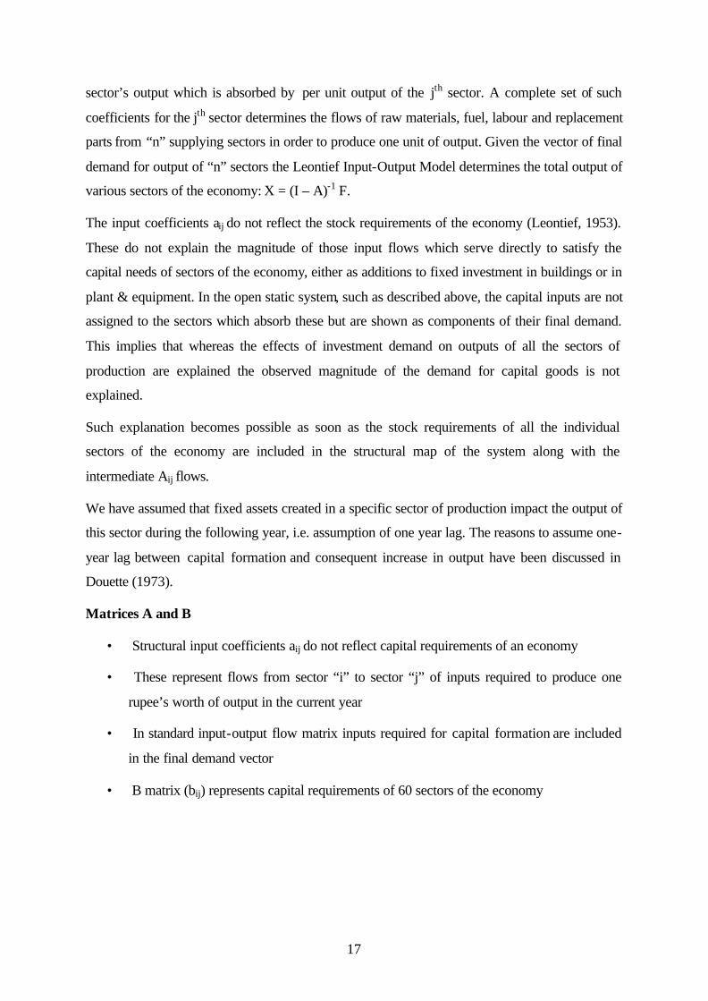
sector’s output which is absorbed by per unit output of the jth sector. A complete set of such

coefficients for the jth sector determines the flows of raw materials, fuel, labour and replacement

parts from “n” supplying sectors in order to produce one unit of output. Given the vector of final

demand for output of “n” sectors the Leontief Input-Output Model determines the total output of

various sectors of the economy: X = (I – A)-1 F.

The input coefficients aij do not reflect the stock requirements of the economy (Leontief, 1953).

These do not explain the magnitude of those input flows which serve directly to satisfy the

capital needs of sectors of the economy, either as additions to fixed investment in buildings or in

plant & equipment. In the open static system, such as described above, the capital inputs are not

assigned to the sectors which absorb these but are shown as components of their final demand.

This implies that whereas the effects of investment demand on outputs of all the sectors of

production are explained the observed magnitude of the demand for capital goods is not

explained.

Such explanation becomes possible as soon as the stock requirements of all the individual

sectors of the economy are included in the structural map of the system along with the

intermediate Aij flows.

We have assumed that fixed assets created in a specific sector of production impact the output of

this sector during the following year, i.e. assumption of one year lag. The reasons to assume one-

year lag between capital formation and consequent increase in output have been discussed in

Douette (1973).

Matrices A and B

• Structural input coefficients aij do not reflect capital requirements of an economy

• These represent flows from sector “i” to sector “j” of inputs required to produce one

rupee’s worth of output in the current year

• In standard input-output flow matrix inputs required for capital formation are included

in the final demand vector

• B matrix (bij) represents capital requirements of 60 sectors of the economy

18

Structural Balance

X = AX + F

X = AX + B ∆X + F

i = 1, 60; j = 1, 60

Xi = Σ aij Xj + Σ bij ∆Xj + Fj

Need for Additional Investment

X1 = a11X1 + a12X2 + b11 ∆X1 + b12 ∆X2 + F1

X2 = a21X1 + a21X2 + b21 ∆X1 + b22 ∆X2 + F2

X1 = (a11+b11) X1+ (a12+b12) X2 – (b11X10+ b12X2

0) + F1

X2 = (a21+b21) X1 + (a22+b22) X2 – (b21X10+ b22X2

0) + F2

Where

∆Xi = Xi – Xi0

bij ∆Xj = ∆Kij is the additional capital requirement of the jth sector for capital good coming from

the ith sector

Details of computing Capital Matrix (B) are provided in Annex-1.

V. Modelling GST

5.1 General Equilibrium Model

We use a general equilibrium model to analyse the impact of India moving towards a

comprehensive GST on goods and services along withy ensuring full tax rebates on exports.

The CGE model that we have developed is distinctly different from existing models of the

Indian economy (Brown et al 1996 and Chadha et al 1998). Our India Model is a single-country,

multi-sectoral CGE model. The present model incorporates some of the features of the new trade

theory, viz. increasing returns to scale, monopolistic competition and product heterogeneity.

India is modelled to produce, consume and 60 goods.

The market structure in 33 manufacturing sectors is modelled as monopolistically competitive.

Perfect competition is assumed in agriculture, mining and service sectors

19

The final demand equations for various sectors are obtained assuming a single representative

consumer who maximises utility subject to a budget constraint. It is assumed that the revenue

from tariffs and indirect taxes gets re-distributed to consumers and then spent. Intermediate

demands are derived from the profit-maximising decisions of the representative firms in each

sector. Products in all the tradable sectors are characterised by some degree of product

differentiation. In the nine sectors where markets are taken to be perfectly competitive, products

are differentiated by country of origin, i.e., whether from India or rest-of-world (ROW). In the

monopolistically competitive industries, products are differentiated by firm. India is assumed to

be a small country such that world prices of various tradable goods are exogenous.

Consumers and producers are assumed to use a two-stage procedure to allocate expenditure

across differentiated products. At the first stage, expenditure is allocated across goods without

regard to the country of origin (whether India or ROW) or the producing firm. At this stage, the

utility function is taken to be Cobb-Douglas and the production function requires intermediate

inputs in fixed proportion. In the second stage, expenditure on monopolistically competitive

goods is allocated across competing firms in India and ROW. However, in the case of perfectly

competitive goods, since individual firm supply is indeterminate, expenditure on each good is

allocated over the industry as a whole. The aggregation function in the second stage is a

Constant Elasticity of Substitution (CES) function. We assume that aggregate expenditure varies

endogenously to hold aggregate employment constant. Such a closure may be thought of as

analogous to the Johansen closure rule.

With respect to factor markets, the variable input requirements are taken to be the same for the

three market structures. Primary and intermediate input aggregates are required in fixed

proportion to output.6 Expenditures on primary inputs are allocated between capital and labour,

assuming that a CES function is used to form the aggregate of these primary inputs. In the case

of the four agricultural sectors, land (along with capital and labour) is also assumed to be one of

the primary factors of production. The primary inputs aggregate in these cases is a CES function

of labour and a CES composite of land and capital. In the monopolistically competitive sectors

as well as in the state monopoly sectors, additional fixed inputs of capital and labour are

required. It is assumed that fixed capital and fixed labour are used in the same proportion as

variable capital and variable labour so that production functions are homothetic. Capital and

labour are assumed to be perfectly mobile across sectors. However, we keep the option of

6 Intermediate inputs include both domestic and imported varieties.

20

specifying sector-specific capital for some purposes, especially for short-term analysis. Land

usage in agriculture is assumed to be substitutable across the four agricultural sectors. Returns to

land, capital and labour are determined to equate factor demand to an exogenous supply of each

factor. The aggregate supplies of labour, capital, and agricultural land are assumed to remain

fixed so as to abstract from macroeconomic considerations involving, for example,

determination of investment, since our focus is on the intersectoral allocation of resources. We

introduce an element of capital coefficients during the base period though its effect on additional

output gets reflected only in the post-simulation new equilibrium values. However, this does not

imply that we increase the base year capital stock in any direct way. In fact, we estimate the

impact of capital coefficients in addition to the input-output structural coefficients.

Perfectly competitive firms are assumed to set price equal to marginal cost, while

monopolistically competitive firms maximise profits by setting price as an optimal mark-up over

marginal cost. The numbers of firms in sectors under monopolistic competition are determined

by the condition that there are zero profits. The price changes are relative to the domestic

numeraire price of the sector “iron and steel”. This price is held constant while solving the

model.

It is assumed that trade remains balanced, i.e. the initial trade imbalance remains constant as

trade barriers are changed. This assumption reflects flexible exchange rate. Moreover, this is an

appropriate way of abstracting from the macroeconomic forces and polices that are the main

determinants of trade imbalance.

This model is solved using GEMPACK (Harrison and Pearson, 1996). The solution of

simulation yields percentage changes in sectoral employment and certain other variables of

interest for India. Multiplying the percentage changes by actual levels given in the data base

yields the absolute changes, positive or negative, that might result from India’s unilateral trade

and domestic policy reforms.

In addition to the sectoral effects that are the primary focus of our analysis, the model also yields

results for changes in exports, imports, the overall level of welfare (measured through GDP) in

the economy, and the economy-wide changes in real wages and returns to land and capital.

Because both labour and capital are assumed to be homogeneous and mobile across sectors in

these scenarios, we cannot distinguish effects on factor prices by sector. Nor can we distinguish

effects on different skill groups or other categories of labour. Though we would like to know

more about the distributional issues associated with the reforms, the model in its present form is

21

not set up to accomplish this. Our model also does not account for changes in foreign direct

investment, and it does not make any allowance for dynamic efficiency changes and economic

growth.

5.2 Simulations Design

The Net Indirect Taxes (NIT) paid by exporters on intermediate purchases (if they are

producer exporters) or NIT passed on to them by producers from whom they purchase the

exportable commodities are supposed to be fully offset. However, the same is not true in

practice. We consider non-offset net indirect taxes as being exported and hence act like

“export tax equivalent” (ETE).

While most of the Central taxes are offset the same is not true at the state-level. In order to

facilitate our analysis we assume non-rebated tax proportions to vary between 25 per cent and

50 per cent (Box-1).

For the present study, we design two sets of simulations, Set-1 and Set-2. While Set-1 refers

to experiments in which export tax equivalents (ETE) are brought down to zero by the full

knocking off the ETE in all the sectors except primary sectors (codes 1-11). The

methodology used is based on standard IOTT “A” matrix. We do not incorporate the

additional impact of capital coefficients in our experiments.

Set-2 refers to the same experiments as in Set-1 but assuming the additional impact of capital

coefficients in our experiments. We use both the “A” and the “B” matrices in S2.1 and S2.2.

The experiments under Set-1 refer to the simulations on providing full tax offsets for the non-

offset component which gets exported through higher export fob price. We assume two

different scenarios as mentioned in Box-1.

The Set-2 of simulations corresponds to those of Set-1 except that these are conducted under

the additional impact of capital coefficients on output of the economy. These parallel

simulations are labelled as S2.1 and S2.2.

As discussed above, our simulations have been designed to study the effect of offsets

experimenting with various scenarios. Under the hypothetical offset of 75 per cent, the

remaining 25 per cent of the ETE is completely eliminated in S1.1 and S2.1. In simulation

S1.2 and S2.2 we assume that there are 50 per cent offsets and that the entire amount of

remaining NIT needs to be eliminated. Our results are presented in Table 2-10.

22

Box-1: Simulations Design

SET 1

S1.1 Export tax equivalents are estimated at 25 per cent of NIT without the effect of capital-coefficients

S1.2 Export tax equivalents are estimated at 50 per cent of NIT without the effect of capital-coefficients

SET 2

S2.1 Export tax equivalents are estimated at 25 per cent of NIT with the additional impact of capital-coefficients

S2.2 Export tax equivalents are estimated at 50 per cent of NIT with the additional impact of capital-coefficients

VI. Results

6.1 Macro Variables: Simulations

In the absence of the additional impact of capital coefficients in the model, the reduction in

ETE of the NIT leads to an improvement in productivity of the economy. The improvement

increases for Simulations under Set 2 as compared with Simulations under Set 1.

Gain in GDP under S1.1 is 0.04 per cent which increases to 0.09 per cent in S1.2 (Table 2).

However, a substantial improvement may be observed when we consider the additional

impact of capital coefficients (Set-2). Here, the gain in GDP increases from 0.87 per cent to

1.7 per cent between S2.1 and S2.2. The gain in growth of GDP is one-time though the

additional absolute return would be perpetual.

The efficiency of energy resource use improves in the new equilibrium. The domestic

consumption of coal, petroleum products and electricity as ratio to GDP goes down from 14.3

per cent to 13.9 per cent. While the GDP grows by 1.7 per cent under scenario S2.2 the usage

of coal & lignite and electricity grows only by 1 per cent each. The usage of petroleum

products declines by 4.5 per cent. The introduction of GST would thus be environment

friendly.

Under Set-1, gain in exports increases from 1.55 per cent to 3.07 per cent between S1.1 and

S1.2. The comparable gains under the additional impact of capital coefficients (Set-2) are

3.22 per cent and 6.34 per cent, respectively.

23

Gains in imports increase from 1.09 per cent in S1.1 to 2.16 per cent in S1.2. Under Set-2 the

corresponding increase is 2.39 per cent to 4.71 per cent, respectively.

Gain in net exports of the economy expands from 0.46 per cent to 0.91 per cent in S1.1 and

S1.2, respectively. Their comparable values in Set-2 are 0.83 per cent to 1.63 per cent.

The economy-wide gain in output expands by 0.21 per cent in S1.1 and by 0.42 per cent in

S1.2. Comparable expansions for Set-2 simulations are 0.32 per cent and 0.64 per cent,

respectively.

Real returns to labour and capital show improvements between the Simulation-1 and

Simulation-2 under both the sets, Set-1 and Set-2. The returns to these factors of production

show substantial improvements with the inclusion of capital coefficients in the model.

Real returns to land deteriorate for both the simulations conducted under Set-1. However, we

get indications of positive real returns to land under simulations of Set-2. This clearly

highlights that land becomes more efficiently allocated in the latter set of experiments.

Using the results, changes in GDP and trade (imports and exports) in absolute values, over

the corresponding values of 2008-09, are provided in Table 3.

6.2 Macro Variable: Comparisons across S1.1, S1.2, S2.1 and S2.2

Gain in absolute value of GDP is Rs. 2,169 crore under S1.1 which increases to Rs. 4,427

crore under S1.2. The corresponding changes in dollar values are $480 million and $979

million, respectively. The results exhibit significant increases under S2.1 and S2.2. Gain in

GDP is Rs. 42,789 crore under S2.1 which increases to Rs. 83,899 crore under S2.2. The

corresponding changes in dollar values are $9,461 million and $18,550 million, respectively.

The additional gain in GDP, originating from the GST reform, would be earned during all

years in future over and above the growth in GDP which would have been achieved

otherwise. The present value of the GST-reform induced gains in GDP may be computed as

the present value of additional income stream based on some discount rate. We assume a

discount rate as the long-term real rate of interest at about 3 per cent. The present va lue of

total gain in GDP has been computed as between Rs. 1,469 thousand crores and 2,881

thousand crores. The corresponding dollar values are $325 billion and $637 billion.

Gains in exports are expected to vary between 3.2 and 6.3 per cent with corresponding

absolute value range as Rs. 24,669 crore and Rs. 48,661 crore. The comparable dollar value

increment is estimated to be between $5,427 million and $10,704 million, respectively.

24

Imports are expected to gain somewhere between 2.4 and 4.7 per cent with corresponding

absolute values ranging between Rs. 31,173 crore and Rs. 61,501 crore. The comparable

dollar value increment is estimated to be between $6,871 million and $13,556 million,

respectively.

6.3 Sectoral Results

We discuss our observations on sectoral output and scale effects for simulation S2.1 and 2.2

(Tables 4 and 5). Results for other simulations have also been presented in these Tables. It

may be observed that output of agricultural sectors shows gains under simulation S2.1as

compared with S1.1 in which output of agricultural sectors shows expected decline. Further

the gains under S2.2 are higher than those observed under S2.1. The largest increases in

output occur in textiles and readymade garments; minerals other than coal, petroleum, gas

and iron ore; organic heavy chemicals; industrial machinery for food and textiles; beverages;

and miscellaneous manufacturing (Table 4). The sectors in which output is expected to

decline include natural gas and crude petroleum; iron ore; coal tar products; and non-ferrous

metal industries. There are minor gains and losses in output of other sectors.

The scale effect (Table 5), which indicates the per cent change in output per firm, is positive

and relatively high for sectors including beverages; textiles and readymade garments; coal tar

products; chemical products; fertilisers; sugar; paints; pesticides; and cement. Scale effects

are positive for all other sectors of manufacturing. Increased output per firm (scale effect) in

the imperfectly competitive manufacturing sectors is an indicator of efficiency gains. The

sectors, in which output grows, the proportional change in output is greater than proportional

increase in number of firms. On the other hand, the sectors, in which output declines, the

proportional decline in output is less than proportional decline in number of firms.

The intersectoral movements of labour and capital are recorded in Tables 6 and 7. Generally,

labour and capital move into the sectors in which output is expected to increase.

The results of our study are based on using capital coefficients computed in B-matrix

(Annex-1). These refer to the registered / organised sectors of the economy. Our analysis in

this study is thus based on the assumption that the capital coefficients computed for the

registered sectors are also applicable to the unregistered sectors. However, it is worthwhile to

compute capital coefficients for unregistered manufacturing sectors also and incorporate the

same in the overall capital matrix. We have not been able to do so due to data limitations.

Using information from the “Unorganised Manufacturing Sector in India: Employment,

25

Assets and Borrowings”, NSSO (2005-06) we have computed some crude estimates of

sectoral as well as overall capital coefficients in the unregistered sector. The aggregate

incremental capital-output ratio turns out to be 1.46 for the unregistered manufacturing

compared with 1.36 for the registered manufacturing sector. Capital coefficients are

significantly high in certain unregistered sectors, viz. food products, textiles, garments,

chemicals and some other manufacturing sectors. It may thus be observed that capital-output

ratios are higher in some of the unregistered sectors than in the registered sectors. The GST

reform would benefit the small-scale and other manufacturing units in unregistered sectors,

relatively more than the corresponding registered sectors, through making capital cheaper

than before through providing the benefits of full tax offsets. The unorganised sector would

thus benefit more than the organised sector as a whole. The same may be true of some of the

sectors within the unorganised sector thus making these more competitive in international

markets than the scenario before the GST reform. The sectors mentioned in this paragraph are

export intensive and hence would add to the exports from India.

6.4 Returns to the Factors of Production

GST would lead to efficient allocation of factors of production. It is expected that the real

returns to the factors of production would go up under the scenarios of Set-2 as compared

with Set-1. Our results for Set-2 show gains in real returns to land ranging between 0.42 and

0.82 per cent. Wage rate gains vary between 0.68 and 1.33 per cent. The real returns to

capital would gain somewhere between 0.37 and 0.74 per cent.

6.5 Exports and Imports

The details of gains in merchandise exports and imports under different scenarios are given in

Tables 8 and 9. Under simulation S2.2 the sectors with the largest proportional change in

exports increases include textiles and readymade garments; beverages; industrial machinery

for food and textiles; transport equipment other than railway equipment; electrical and

electronic machinery; and chemical products: organic and inorganic. The moderate gainers

are agricultural machinery; metal products; other machinery; and railway transport

equipment. Exports are expected to decline in agricultural sectors; iron and steel; wood and

wood products except furniture; and cement. There are minor gains and losses in exports of

other sectors (Table 8).

The major import gaining sectors include leather and leather products; furniture and fixtures;

agricultural sectors; coal and lignite; agricultural machinery; industrial machinery; other

26

machinery; iron and steel; railway transport equipment; printing and publishing; and tobacco

products. The moderate gainers include metal products; non-ferrous metals; and transport

equipment other than railways. Imports are expected to decline in textiles and readymade

garments; minerals other than coal, crude petroleum, gas and iron ore; and beverages (Table

9).

6.6 Changes in Prices

There are two opposing forces which determine the changes in price levels. First, increased

payments to the primary factors of production, viz. land, labour and capital, increase the cost

of production and hence tend to have upward pull on prices. Second, sectors under imperfect

competition (manufacturing sectors) get benefits of cost reduction through increasing returns

to scale which are not reaped by sectors assumed to be in perfect competition. The relative

impact of the force determines the overall price change. It may also be noted that the share of

primary inputs (land, labour and capital) in total output is relatively high in agricultural and

services sectors.

Another factor that impacts the price levels refers to the quantum of intermediate input

purchases from sectors under perfect competition versus imperfect competition. Relatively

low proportions of intermediate inputs purchased by agriculture and service sectors (i.e.

sectors under perfect competition) are sourced from manufacturing sectors and hence these

sectors do not reap the benefit of relatively low cost inputs from manufacturing sectors.

Terms of trade would improve in favour of agriculture vis-à-vis manufactured goods. The

overall prices of agricultural goods (Sectors 1 - 7) go up by 0.57 per cent under S-2.1 and by

1.12 per cent under S-2.2. The overall prices of all the manufacturing sectors (sectors 12 - 44)

decline by 1.22 per cent under S-2.1 and by 2.53 per cent under S-2.2. Consequently, the

terms-of-trade move in favour of agriculture vis-à-vis manufactured goods within a range of

1.8 to 3.8 per cent.

The increase in agricultural prices would benefit millions of farmers in India. With regard to

the food crops the poor would continue to remain secured through the public distribution

system. The prices of many other consumer goods are expected to decline. These include

sugar; beverages; cotton textiles; wool, silk and synthetic fibre textiles; and textile products

and wearing apparel.

N.C.: Not Computed; Sectors 45, 46, 47, 50, 56, 57, 58 and 60 are not internationally traded

(IO 2003-04) and hence the changes in their prices could not be computed.

27

6.7 Net Indirect Tax and Gains in Exports

We have computed regression equation with percentage change in exports as dependent

variable and “net indirect tax to output ratio (NIT-to-Q ratio)” as independent variable.

Results show positive and significant relationship between percentage changes in exports to

NIT-to-Q ratio. This is indicative of the fact that full tax offsets in relatively high taxed

sectors would lead to higher gains in exports compared to less taxed sectors.

VII. Revenue Neutral GST Rate

Based on the results of our simulations, we have attempted to determine a uniform revenue-

neutral GST rate. This implies computation of GST rate which results in the same net indirect

revenue as collected in 2003-04, i.e. the IOTT used in this study. The total NIT was 2,16,073

crore. The revenue neutrality exercise has been undertaken for the simulations S2.1 and S2.2.

The model does not have details on government budget. It abstracts from macroeconomic

variables

The output tax rates (row-wise) are given in Table 11.7 However, given the sensitivity of the

subsided sectors, i.e. sectors with negative NIT values, our computations have excluded such

sectors from the ambit of computing the revenue neutral GST rate. We have conducted two

alternative exercises:

1. Applying GST to all the sectors of goods and services excluding sectors: food crops (01);

cash crops (02); plantation crops (03); other crops (04); and fertilizers (30).

2. Applying GST to all the goods and services sectors excluding sectors: fishing (07);

electricity (46); railway transport services (48); and communication (51) over and

above those mentioned in Scenario-1.

3. Applying GST to all goods and services sectors excluding food crops (01), education and

research (57) and medical and health (58). Under the assumption that the petroleum

tax would not be subsumed in GST, the base tax value has been adjusted through

subtracting the NIT on output of petroleum products from total NIT. The total NIT is

Rs.2,16,073 crore. The NIT on output of petroleum products (IO sector 26) is

Rs.39,184 crore. Thus, the revised base tax after excluding NIT for the petroleum

products is Rs.1,76,889 crore.

7 We do not assume any exemptions on indirect taxes paid on final consumption in our computations. The GST rate would be higher than what we have computed if there are some exemptions for taxing consumption of certain goods and services.

28

4. Applying GST on all goods and services (no exemptions) with initial tax base being same

as in Scenario-3.

The computation of revenue neutrality is based on taxing all the goods and services going to

final consumption, i.e. “final demand net of change in stocks minus exports plus imports

(excluding imports going for intermediate usage)”. We have attempted two different variants.

The results of these four cases are tabulated in Box-2. Based on our computations, the

revenue neutral GST rate across goods and services is expected to be positioned somewhere

in the range of 6.2 per cent and 9.4 per cent, depending on various scenarios of sectoral

exemptions. GST rates of some other countries are shown in Figure-5.

Box 2: Revenue Neutral GST Rates

Revenue Neutral GST Rate (%) Group Excluded IO sectors

S2.1 S2.2

1 Food crops (01), Cash crops (02), Plantation crops (03), Other crops (04), Fertilizers ( 30)

9.04 9.01

2 Food crops (01), Cash crops (02), Plantation crops (03), Other crops (04), Fishing (07), Fertilizers (30), Electricity (46), Railway transport services (48), Communication (51)

9.42 9.40

3* Food crops (01), Education and research (57), Medical and health (58)

7.25 7.22

4* None 6.22 6.20 * In scenario 3 and 4, the revised base tax has been computed after excluding NIT on output of petroleum products (IO 26) from total NIT. S2.1: Export tax equivalents are reduced by 25 per cent with additional impact of capital-coefficients. S2.2 Export tax equivalents are reduced by 50 per cent with additional impact of capital-coefficients. Source: NCAER computations

29

VIII. Concluding Remarks

Implementation of a comprehensive GST across goods and services is expected, ceteris

paribus, to increase India’s GDP somewhere within a range of 0.9 per cent to 1.7 per cent.

The corresponding changes in absolute values of GDP over 2008-09 is expected to be

between Rs. 42,789 crore and Rs. 83,899 crore, respectively. The comparable dollar value

increment is estimated to be between $9,461 million and $18,550 million, respectively.

The additional gain in GDP, originating from the GST reform, would be earned during all

years in future over and above the growth in GDP which would have been achieved

otherwise. The present value of the GST-reform induced gains in GDP may be computed as

the present value of additional income stream based on some discount rate. We assume a

discount rate as the long-term real rate of interest at about 3 per cent. The present value of

total gain in GDP has been computed as between Rs. 1,469 thousand crores and 2,881

thousand crores. The corresponding dollar values are $325 billion and $637 billion.

Gains in exports are expected to vary between 3.2 and 6.3 per cent with corresponding

absolute value range as Rs. 24,669 crore and Rs. 48,661 crore. The comparable dollar value

increment is estimated to be between $5,427 million and $10,704 million, respectively.

Imports are expected to gain somewhere between 2.4 and 4.7 per cent with corresponding

absolute values ranging between Rs. 31,173 crore and Rs. 61,501 crore. The comparable

dollar value increment is estimated to be between $6,871 million and $13,556 million,

respectively.

Figure-5: Country-wise GST Rates

0

5

10

15

20

25

Sing

apor

e

Can

ada

Tha

iland

Aus

tral

ia

Indo

nesi

a

Phili

ppin

es

New

Zea

land

Chi

na UK

Ger

man

y

Fran

ce

Bel

gium

Per

cent

Source: websearch

30

GST would lead to efficient allocation of factors of production. The overall price level would

go down. It is expected that the real returns to the factors of production would go up. Our

results show gains in real returns to land ranging between 0.42 and 0.82 per cent. Wage rate

gains vary between 0.68 and 1.33 per cent. The real returns to capital would gain somewhere

between 0.37 and 0.74 per cent.

The efficiency of energy resource use improves in the new equilibrium. The introduction of

GST would thus be environment friendly.

Based on our computations, the revenue neutral GST rate across goods and services is

expected to be positioned somewhere in the range of 6.2 per cent and 9.4 per cent, depending

on various scenarios of sectoral exemptions.

In sum, implementation of a comprehensive GST in India is expected to lead to efficient

allocation of factors of production thus leading to gains in GDP and exports. This would

translate into enhanced economic welfare and returns to the factors of production, viz. land,

labour and capital.

As with any other modelling exercise, the results of our exercise are subject to certain

limitations. The general equilibrium model that we have used is comparative static in nature.

Aggregate supplies of labour, capital, and agricultural land are assumed to remain fixed so as to

abstract from macroeconomic considerations. Given these limitations the results must not be

read as forecasts of variables but only as indicative directional changes.

31

Table 1: Distribution of Net Indirect Tax (NIT) across Sectors: Column-wise (Rs. Lakh)

Non-Offset Component of

NIT/Q*

IO Code Description NIT Output

NIT/Q (%)

25% for all sectors

50% for all

sectors 01 Food crops -2459549 24018772 -10.24 - - 02 Cash crops -799381 8415368 -9.50 - - 03 Plantation crops -21715 6158859 -0.35 - - 04 Other crops -1319582 14717186 -8.97 - - 05 Animal husbandry 58446 18281531 0.32 0.08 0.16 06 Forestry & logging 10162 2486237 0.41 0.10 0.20 07 Fishing 5148 3171641 0.16 0.04 0.08 08 Coal and lignite 63565 3504984 1.81 0.45 0.91 09 Natural gas & Crude Petroleum 70976 3417653 2.08 0.52 1.04 10 Iron ore 8916 466676 1.91 0.48 0.96 11 Other minerals 18619 1362604 1.37 0.34 0.68 12 Sugar 36082 3347510 1.08 0.27 0.54 13 Food products excluding sugar 310823 18862942 1.65 0.41 0.82 14 Beverages 125281 2578789 4.86 1.21 2.43 15 Tobacco products 75711 1146560 6.60 1.65 3.30 16 Cotton textiles 127337 5775566 2.20 0.55 1.10

17 Wool, silk & synthetic fibre textiles 167616 3779899 4.43 1.11 2.22

18 Jute, hemp and mesta textiles 6292 448282 1.40 0.35 0.70

19 Textiles products including wearing apparel 249570 8352802 2.99 0.75 1.49

20 Wood and wood products except furniture 15137 848314 1.78 0.45 0.89

21 Furniture and fixture 31336 817397 3.83 0.96 1.92 22 Paper and paper products 157595 2413073 6.53 1.63 3.27

23 Printing, publishing and allied activities 134929 2093160 6.45 1.61 3.22

24 Leather and leather products 72760 1633695 4.45 1.11 2.23 25 Plastic and rubber products 367018 6013,370 6.10 1.53 3.05 26 Petroleum products 1648626 17375676 9.49 2.37 4.74 27 Coal tar products 45531 829162 5.49 1.37 2.75 28 Inorganic heavy chemicals 198546 2926687 6.78 1.70 3.39 29 Organic heavy chemicals 182309 2495675 7.30 1.83 3.65 30 Fertilizers 170890 3200493 5.34 1.33 2.67 31 Paints, varnishes and lacquers 132469 1762397 7.52 1.88 3.76

32 Pesticides, drugs and other chemicals 1025062 14640229 7.00 1.75 3.50

33 Cement 52996 1897034 2.79 0.70 1.40 34 Non metallic mineral products 199323 4045898 4.93 1.23 2.46 35 Iron & steel industries and 748355 13749377 5.44 1.36 2.72

32

Non-Offset Component of

NIT/Q*

IO Code Description NIT Output

NIT/Q (%)

25% for all sectors

50% for all

sectors foundries

36 Other basic metal industry 154267 2979788 5.18 1.29 2.59

37 Metal products except mach & transport Equipment 371203 5798872 6.40 1.60 3.20

38 Agricultural machinery 79857 1048495 7.62 1.90 3.81

39 Industrial machinery for food and textiles 66534 823870 8.08 2.02 4.04

40 Other machinery 559456 7662699 7.30 1.83 3.65

41 Electrical, electronic machinery & appliances 1317141 16443198 8.01 2.00 4.01

42 Railway transport equipment 55629 865713 6.43 1.61 3.21 43 Other transport equipment 638423 9216468 6.93 1.73 3.46

44 Miscellaneous manufacturing industries 336979 7100046 4.75 1.19 2.37

45 Construction 2339910 44152788 5.30 1.32 2.65 46 Electricity -948373 14790883 -6.41 - - 47 Water supply 4121 786315 0.52 0.13 0.26 48 Railway transport services -158825 5513456 -2.88 - - 49 Other transport services 2178276 36359410 5.99 1.50 3.00 50 Storage and warehousing 3952 308332 1.28 0.32 0.64 51 Communication -102072 5728231 -1.78 - - 52 Trade 278957 45422021 0.61 0.15 0.31 53 Hotels and restaurants 198573 10292468 1.93 0.48 0.96 54 Banking 67202 16842287 0.40 0.10 0.20 55 Insurance 52977 4239538 1.25 0.31 0.62 56 Ownership of dwellings 14181 13931500 0.10 0.03 0.05 57 Education and research 27015 10887331 0.25 0.06 0.12 58 Medical and health 261743 7301778 3.58 0.90 1.79 59 Other services 176794 21413849 0.83 0.21 0.41

60 Public administration and defence 0 15615700 0.00 0.00 0.00

Total 9891117 512560534 1.91 0.00 0.00 * Non-Offset Component of NIT at 25% implies that the total NIT paid has been offset to the extent of 75%. Similarly, Non-Offset Component of NIT at 50% implies that the total NIT paid has been offset to the extent of 50%. Source: NCAER computation based on IO 2003-04. Sectors with subsidy (negative NIT/Output ratio) are not considered in computations in this Table.

33

Table 2: Percentage Change in Macro Variables

SET 1: Without

Capital Coefficients SET 2: With

Capital Coefficients S. No. Sector Description S 1.1 S 1.2 S 2.1 S 2.2

Non Offset NIT Rate (25%) (50%) (25%) (50%)

1 GDP 0.04 0.09 0.87 1.70

2 Export 1.55 3.07 3.22 6.34

3 Import 1.09 2.16 2.39 4.71

4 Net Export 0.46 0.91 0.83 1.63

5 Output 0.21 0.42 0.32 0.64

6 Real Returns to Land -0.06 -0.11 0.42 0.82

7 Real Returns to Labour 0.12 0.24 0.68 1.33

8 Real Returns to Capital 0.34 0.68 0.37 0.74 Source: NCAER Simulations

34

Table 3: Absolute Changes in Macro Variables over 2008-09 Values

SET 1: Without Capital

Coefficients

SET 2: With Capital

Coefficients S. No.

Sector Description S 1.1 S 1.2 S 2.1 S 2.2

Non Offset NIT Rate

Values: 2008-09 (25%) (50%) (25%) (50%)

Rs. Crore 1 GDP 49,33,183 2,169 4,427 42,789 83,899 2 Export 7,66,935 11,859 23,547 24,669 48,661 3 Import 13,05,503 14,165 28,158 31,173 61,501 4 Net Export -5,38,568 -2,484 -4,919 -4,464 -8,800

US$ Million 1 GDP 1,090,734 480 979 9,461 18,550 2 Export 168,704 2,609 5,180 5,427 10,704 3 Import 287,759 3,122 6,207 6,871 13,556 4 Net Export -119,055 -549 -1,087 -987 -1,945

Source: NCAER Simulations

35

Table 4: Percentage Change in Output

SET 1: Without

Capital Coefficients SET 2: With Capital

Coefficients S. No. Sector Description S 1.1 S 1.2 S 2.1 S 2.2 Non Offset NIT Rate (25%) (50%) (25%) (50%)

1 Food crops -0.09 -0.17 0.19 0.36 2 Cash crops -0.09 -0.17 1.25 2.46 3 Plantation crops -0.14 -0.28 0.03 0.04 4 Other crops -0.04 -0.08 0.06 0.11 5 Animal husbandry -0.04 -0.09 0.40 0.78 6 Forestry & logging -0.19 -0.38 -1.18 -2.31 7 Fishing -0.46 -0.91 0.54 1.04 8 Coal and lignite 0.01 0.01 -0.43 -0.85 9 Natural gas & Crude Petroleum -1.43 -2.86 -3.63 -7.17

10 Iron ore -1.15 -2.29 -2.89 -5.69 11 Other minerals 2.82 5.61 9.21 18.13 12 Sugar -0.14 -0.27 1.47 2.88 13 Food products excluding sugar -0.34 -0.66 0.62 1.20 14 Beverages -0.10 -0.20 3.06 6.00 15 Tobacco products -0.09 -0.18 0.54 1.05 16 Cotton textiles -0.52 -0.94 6.22 12.26 17 Wool, silk & synthetic fibre textiles 1.29 2.63 11.06 21.78 18 Jute, hemp and mesta textiles -0.32 -0.63 0.81 1.58

19 Textiles products including wearing apparel -0.10 0.03 16.71 32.99

20 Wood and wood products except furniture -0.08 -0.17 -1.00 -1.96 21 Furniture and fixture 0.13 0.25 0.53 1.03 22 Paper and paper products -0.01 -0.03 1.03 2.01 23 Printing, publishing and allied activities -0.11 -0.22 0.70 1.37 24 Leather and leather products 0.68 1.34 0.12 0.25 25 Plastic and rubber products 0.63 1.25 1.88 3.68 26 Petroleum products 0.54 1.06 1.31 2.55 27 Coal tar products -0.27 -0.55 -2.13 -4.18 28 Inorganic heavy chemicals 0.65 1.27 2.12 4.14 29 Organic heavy chemicals 4.26 8.33 5.65 11.03 30 Fertilizers 0.12 0.23 1.27 2.49 31 Paints, varnishes and lacquers 0.75 1.46 1.06 2.08 32 Pesticides, drugs and other chemicals 0.75 1.46 1.93 3.78 33 Cement 0.13 0.26 -0.63 -1.23 34 Non metallic mineral products 0.19 0.36 -0.25 -0.49 35 Iron & steel industries and foundries 0.90 1.76 -0.23 -0.46 36 Other basic metal industry 2.09 4.05 -2.30 -4.55

37 Metal products except mach & transport Equipment 0.63 1.23 0.70 1.36

38 Agricultural machinery 0.34 0.67 0.33 0.65 39 Industrial machinery for food and textiles 0.29 0.59 3.99 7.84 40 Other machinery 0.63 1.21 -0.23 -0.47

36

SET 1: Without

Capital Coefficients SET 2: With Capital

Coefficients S. No. Sector Description S 1.1 S 1.2 S 2.1 S 2.2 Non Offset NIT Rate (25%) (50%) (25%) (50%)

41 Electrical, electronic machinery & appliances 0.59 1.14 0.61 1.19

42 Railway transport equipment 0.19 0.38 0.43 0.84 43 Other transport equipment 0.49 0.96 1.21 2.37 44 Miscellaneous manufacturing industries 9.09 17.94 3.00 6.00 45 Construction 0.11 0.21 -3.52 -6.88 46 Electricity 0.17 0.34 0.68 1.33 47 Water supply -0.02 -0.05 0.01 0.02 48 Railway transport services 0.21 0.41 -0.19 -0.37 49 Other transport services -0.02 -0.04 0.82 1.60 50 Storage and warehousing -0.11 -0.21 0.02 0.03 51 Communication 0.14 0.27 0.61 1.19 52 Trade -0.19 -0.37 0.31 0.61 53 Hotels and restaurants -0.30 -0.60 0.07 0.13 54 Banking 0.06 0.12 0.37 0.73 55 Insurance -0.10 -0.20 0.41 0.81 56 Ownership of dwellings -0.16 -0.32 -6.10 -11.92 57 Education and research -0.11 -0.21 0.42 0.82 58 Medical and health 0.02 0.05 -2.22 -4.35 59 Other services -0.78 -1.56 -1.84 -3.63 60 Public administration and defence -0.01 -0.03 0.22 0.43

Total 0.21 0.42 0.32 0.64

Note: Increase and decrease in output results from full employment and resource use in the economy. Results are based on resource re-allocation across sectors. Source: NCAER Simulations

37

Table 5: Percentage Change in Output per Firm: Scale Effects

SET 1: Without Capital

Coefficients

SET 2: With Capital

Coefficients S. No. Sector Description S 1.1 S 1.2 S 2.1 S 2.2

Non Offset NIT Rate (25%) (50%) (25%) (50%) 1 Food crops - - - - 2 Cash crops - - - - 3 Plantation crops - - - - 4 Other crops - - - - 5 Animal husbandry - - - - 6 Forestry & logging - - - - 7 Fishing - - - - 8 Coal and lignite - - - - 9 Natural gas & Crude Petroleum - - - - 10 Iron ore - - - - 11 Other minerals - - - - 12 Sugar 0.05 0.10 1.22 2.40 13 Food products excluding sugar 0.04 0.07 0.68 1.34 14 Beverages 0.06 0.12 2.90 5.68 15 Tobacco products 0.04 0.08 0.11 0.21 16 Cotton textiles 0.04 0.08 1.69 3.32 17 Wool, silk & synthetic fibre textiles 0.38 0.77 2.73 5.37 18 Jute, hemp and mesta textiles 0.06 0.13 0.90 1.76 19 Textiles products including wearing apparel 0.10 0.23 2.86 5.62 20 Wood and wood products except furniture 0.20 0.40 0.27 0.54 21 Furniture and fixture 0.26 0.51 0.45 0.88 22 Paper and paper products 0.18 0.35 0.93 1.83 23 Printing, publishing and allied activities 0.21 0.41 0.85 1.67 24 Leather and leather products 0.18 0.35 0.46 0.90 25 Plastic and rubber products 0.41 0.81 1.36 2.67 26 Petroleum products 0.57 1.13 1.14 2.24 27 Coal tar products 0.32 0.63 1.30 2.54 28 Inorganic heavy chemicals 0.49 0.97 1.56 3.06 29 Organic heavy chemicals 0.52 1.02 1.59 3.13 30 Fertilizers 0.48 0.94 1.65 3.23 31 Paints, varnishes and lacquers 0.47 0.92 1.30 2.55 32 Pesticides, drugs and other chemicals 0.48 0.94 1.24 2.43 33 Cement 0.26 0.51 1.06 2.09 34 Non metallic mineral products 0.26 0.51 1.12 2.20 35 Iron & steel industries and foundries 0.35 0.68 0.51 1.01 36 Other basic metal industry 0.48 0.96 0.88 1.73

37 Metal products except mach & transport Equipment 0.41 0.81 0.57 1.12

38 Agricultural machinery 0.37 0.72 0.63 1.24 39 Industrial machinery for food and textiles 0.41 0.81 0.64 1.26 40 Other machinery 0.39 0.76 0.53 1.04

38

SET 1: Without Capital

Coefficients

SET 2: With Capital

Coefficients S. No. Sector Description S 1.1 S 1.2 S 2.1 S 2.2

Non Offset NIT Rate (25%) (50%) (25%) (50%) 41 Electrical, electronic machinery & appliances 0.47 0.93 0.74 1.45 42 Railway transport equipment 0.32 0.63 0.48 0.94 43 Other transport equipment 0.34 0.66 0.54 1.07 44 Miscellaneous manufacturing industries 0.93 1.84 1.09 2.15 45 Construction - - - - 46 Electricity - - - - 47 Water supply - - - - 48 Railway transport services - - - - 49 Other transport services - - - - 50 Storage and warehousing - - - - 51 Communication - - - - 52 Trade - - - - 53 Hotels and restaurants - - - - 54 Banking - - - - 55 Insurance - - - - 56 Ownership of dwellings - - - - 57 Education and research - - - - 58 Medical and health - - - - 59 Other services - - - - 60 Public administration and defence - - - -

Source: NCAER Simulations

39

Table 6: Percentage Change in Employment

SET 1: Without Capital

Coefficients

SET 2: With Capital

Coefficients S. No. Sector Description S 1.1 S 1.2 S 2.1 S 2.2

Non Offset NIT Rate (25%) (50%) (25%) (50%) 1 Food crops -0.10 -0.21 0.05 0.09 2 Cash crops -0.13 -0.24 1.13 2.21 3 Plantation crops -0.17 -0.34 -0.10 -0.21 4 Other crops -0.08 -0.16 -0.07 -0.14 5 Animal husbandry -0.07 -0.15 0.27 0.53 6 Forestry & logging -0.22 -0.44 -1.30 -2.56 7 Fishing -0.29 -0.57 0.30 0.57 8 Coal and lignite 0.21 0.40 -0.69 -1.37 9 Natural gas & Crude Petroleum -1.24 -2.48 -3.90 -7.69 10 Iron ore -0.95 -1.90 -3.15 -6.21 11 Other minerals 3.02 6.00 8.94 17.61 12 Sugar -0.08 -0.15 1.20 2.35 13 Food products exc luding sugar -0.27 -0.54 0.42 0.82 14 Beverages -0.03 -0.05 2.51 4.92 15 Tobacco products -0.01 -0.03 0.40 0.77 16 Cotton textiles -0.46 -0.82 5.87 11.58 17 Wool, silk & synthetic fibre textiles 1.34 2.72 10.50 20.69 18 Jute, hemp and mesta textiles -0.25 -0.49 0.56 1.11 19 Textiles products including wearing apparel 0.01 0.25 16.11 31.80 20 Wood and wood products except furniture -0.11 -0.22 -1.28 -2.51 21 Furniture and fixture 0.09 0.17 0.17 0.33 22 Paper and paper products 0.21 0.41 0.55 1.07 23 Printing, publishing and allied activities -0.02 -0.04 0.17 0.31 24 Leather and leather products 0.74 1.46 -0.18 -0.35 25 Plastic and rubber products 0.72 1.41 1.48 2.89 26 Petroleum products 0.59 1.16 0.95 1.85 27 Coal tar products -0.23 -0.47 -2.44 -4.79 28 Inorganic heavy chemicals 0.73 1.43 1.67 3.27 29 Organic heavy chemicals 4.34 8.49 5.19 10.15 30 Fertilizers 0.23 0.44 0.78 1.52 31 Paints, varnishes and lacquers 0.83 1.63 0.65 1.28 32 Pesticides, drugs and other chemicals 0.83 1.63 1.53 2.99 33 Cement 0.25 0.49 -1.01 -1.96 34 Non metallic mineral products 0.30 0.59 -0.63 -1.24 35 Iron & steel industries and foundries 0.97 1.91 -0.48 -0.95 36 Other basic metal industry 2.11 4.08 -2.55 -5.04

37 Metal products except mach & transport Equipment 0.67 1.31 0.47 0.92

38 Agricultural machinery 0.49 0.96 -0.04 -0.08 39 Industrial machinery for food and textiles 0.43 0.87 3.62 7.11 40 Other machinery 0.76 1.47 -0.61 -1.21

40

SET 1: Without Capital

Coefficients

SET 2: With Capital

Coefficients S. No. Sector Description S 1.1 S 1.2 S 2.1 S 2.2

Non Offset NIT Rate (25%) (50%) (25%) (50%) 41 Electrical, electronic machinery & appliances 0.86 1.68 0.03 0.05 42 Railway transport equipment 0.30 0.58 0.15 0.30 43 Other transport equipment 0.62 1.20 0.89 1.75 44 Miscellaneous manufacturing industries 9.27 18.27 2.41 4.85 45 Construction 0.18 0.36 -3.63 -7.09 46 Electricity 0.26 0.51 0.56 1.10 47 Water supply 0.06 0.12 -0.11 -0.21 48 Railway transport services 0.29 0.56 -0.29 -0.57 49 Other transport services 0.17 0.32 0.56 1.10 50 Storage and warehousing 0.04 0.07 -0.18 -0.34 51 Communication 0.29 0.56 0.40 0.79 52 Trade 0.04 0.08 0.00 0.01 53 Hotels and restaurants -0.09 -0.17 -0.22 -0.45 54 Banking 0.24 0.47 0.13 0.25 55 Insurance 0.08 0.15 0.17 0.33 56 Ownership of dwellings 0.03 0.06 -6.37 -12.44 57 Education and research 0.02 0.05 0.24 0.47 58 Medical and health 0.16 0.31 -2.41 -4.70 59 Other services -0.65 -1.30 -2.03 -3.99 60 Public administration and defence -0.01 -0.03 0.22 0.43

Source: NCAER Simulations

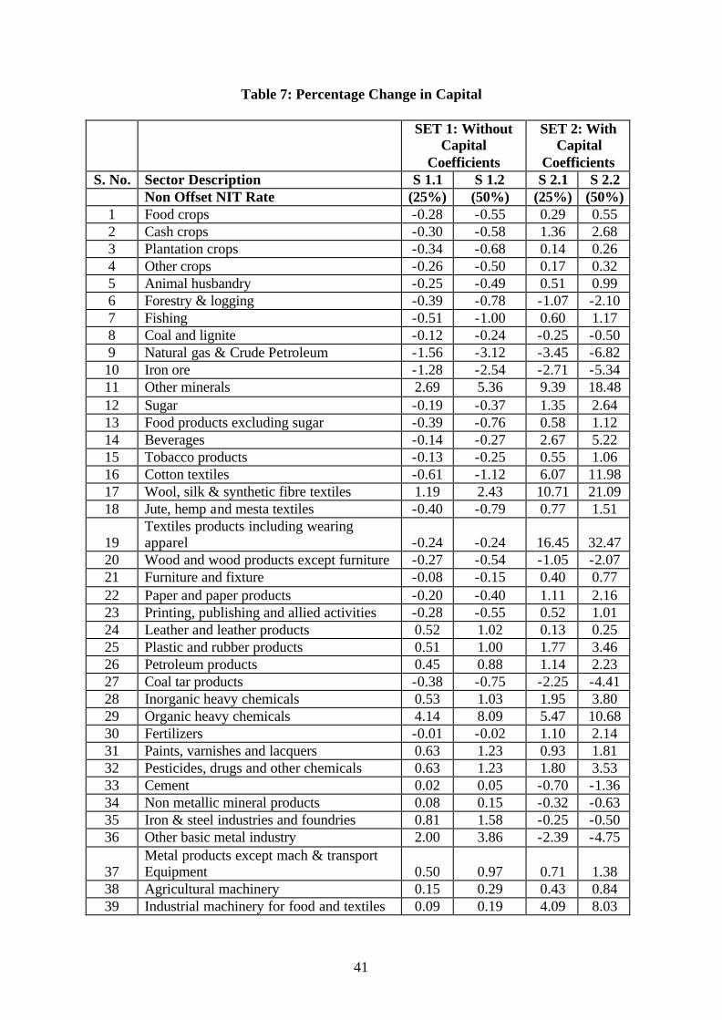
41

Table 7: Percentage Change in Capital

SET 1: Without Capital

Coefficients

SET 2: With Capital

Coefficients S. No. Sector Description S 1.1 S 1.2 S 2.1 S 2.2

Non Offset NIT Rate (25%) (50%) (25%) (50%) 1 Food crops -0.28 -0.55 0.29 0.55 2 Cash crops -0.30 -0.58 1.36 2.68 3 Plantation crops -0.34 -0.68 0.14 0.26 4 Other crops -0.26 -0.50 0.17 0.32 5 Animal husbandry -0.25 -0.49 0.51 0.99 6 Forestry & logging -0.39 -0.78 -1.07 -2.10 7 Fishing -0.51 -1.00 0.60 1.17 8 Coal and lignite -0.12 -0.24 -0.25 -0.50 9 Natural gas & Crude Petroleum -1.56 -3.12 -3.45 -6.82 10 Iron ore -1.28 -2.54 -2.71 -5.34 11 Other minerals 2.69 5.36 9.39 18.48 12 Sugar -0.19 -0.37 1.35 2.64 13 Food products excluding sugar -0.39 -0.76 0.58 1.12 14 Beverages -0.14 -0.27 2.67 5.22 15 Tobacco products -0.13 -0.25 0.55 1.06 16 Cotton textiles -0.61 -1.12 6.07 11.98 17 Wool, silk & synthetic fibre textiles 1.19 2.43 10.71 21.09 18 Jute, hemp and mesta textiles -0.40 -0.79 0.77 1.51

19 Textiles products including wearing apparel -0.24 -0.24 16.45 32.47

20 Wood and wood products except furniture -0.27 -0.54 -1.05 -2.07 21 Furniture and fixture -0.08 -0.15 0.40 0.77 22 Paper and paper products -0.20 -0.40 1.11 2.16 23 Printing, publishing and allied activities -0.28 -0.55 0.52 1.01 24 Leather and leather products 0.52 1.02 0.13 0.25 25 Plastic and rubber products 0.51 1.00 1.77 3.46 26 Petroleum products 0.45 0.88 1.14 2.23 27 Coal tar products -0.38 -0.75 -2.25 -4.41 28 Inorganic heavy chemicals 0.53 1.03 1.95 3.80 29 Organic heavy chemicals 4.14 8.09 5.47 10.68 30 Fertilizers -0.01 -0.02 1.10 2.14 31 Paints, varnishes and lacquers 0.63 1.23 0.93 1.81 32 Pesticides, drugs and other chemicals 0.63 1.23 1.80 3.53 33 Cement 0.02 0.05 -0.70 -1.36 34 Non metallic mineral products 0.08 0.15 -0.32 -0.63 35 Iron & steel industries and foundries 0.81 1.58 -0.25 -0.50 36 Other basic metal industry 2.00 3.86 -2.39 -4.75

37 Metal products except mach & transport Equipment 0.50 0.97 0.71 1.38

38 Agricultural machinery 0.15 0.29 0.43 0.84 39 Industrial machinery for food and textiles 0.09 0.19 4.09 8.03

42

SET 1: Without Capital

Coefficients

SET 2: With Capital

Coefficients S. No. Sector Description S 1.1 S 1.2 S 2.1 S 2.2

Non Offset NIT Rate (25%) (50%) (25%) (50%) 40 Other machinery 0.42 0.80 -0.14 -0.30

41 Electrical, electronic machinery & appliances 0.36 0.69 0.72 1.40

42 Railway transport equipment 0.05 0.09 0.49 0.96 43 Other transport equipment 0.37 0.71 1.23 2.41 44 Miscellaneous manufacturing industries 8.76 17.28 3.11 6.20 45 Construction -0.19 -0.37 -3.12 -6.10 46 Electricity -0.07 -0.13 1.00 1.96 47 Water supply -0.26 -0.52 0.34 0.66 48 Railway transport services 0.02 0.04 0.08 0.14 49 Other transport services -0.10 -0.20 0.93 1.81 50 Storage and warehousing -0.23 -0.46 0.19 0.37 51 Communication 0.02 0.04 0.77 1.50 52 Trade -0.23 -0.45 0.37 0.72 53 Hotels and restaurants -0.35 -0.70 0.14 0.26 54 Banking -0.03 -0.06 0.49 0.96 55 Insurance -0.19 -0.38 0.54 1.04 56 Ownership of dwellings -0.23 -0.46 -6.00 -11.72 57 Education and research -0.24 -0.48 0.61 1.18 58 Medical and health -0.11 -0.22 -2.04 -3.99 59 Other services -0.92 -1.82 -1.66 -3.28 60 Public administration and defence -0.28 -0.55 0.59 1.15

Source: NCAER Simulations

43

Table 8: Percentage Change in Export

SET 1: Without Capital

Coefficients

SET 2: With Capital

Coefficients S. No. Sector Description S 1.1 S 1.2 S 2.1 S 2.2

Non Offset NIT Rate (25%) (50%) (25%) (50%) 1 Food crops -1.99 -3.96 -5.52 -10.86 2 Cash crops -1.96 -3.89 -5.69 -11.20 3 Plantation crops -1.87 -3.71 -5.94 -11.68 4 Other crops -1.93 -3.84 -6.05 -11.90 5 Animal husbandry -2.03 -4.02 -5.43 -10.68 6 Forestry & logging -1.69 -3.37 -6.39 -12.55 7 Fishing -2.48 -4.91 -3.27 -6.46 8 Coal and lignite -1.92 -3.81 -4.68 -9.21 9 Natural gas & Crude Petroleum -0.61 -1.21 -1.49 -2.94 10 Iron ore -1.88 -3.72 -4.48 -8.82 11 Other minerals 0.63 1.25 1.42 2.80 12 Sugar -1.81 -3.57 -0.70 -1.39 13 Food products excluding sugar -1.52 -3.00 -2.14 -4.20 14 Beverages 0.94 1.85 7.13 13.98 15 Tobacco products 2.19 4.27 0.49 0.92 16 Cotton textiles -3.13 -5.87 17.63 34.86 17 Wool, silk & synthetic fibre textiles 7.55 15.21 39.16 77.14 18 Jute, hemp and mesta textiles -3.85 -7.58 -4.38 -8.59

19 Textiles products including wearing apparel -0.13 0.22 33.98 67.12

20 Wood and wood products except furniture -0.47 -0.93 -3.68 -7.21 21 Furniture and fixture 1.08 2.13 -1.32 -2.57 22 Paper and paper products 2.96 5.79 2.68 5.24 23 Printing, publishing and allied activities 2.76 5.40 1.88 3.67 24 Leather and leather products 1.90 3.75 -0.81 -1.57 25 Plastic and rubber products 3.57 7.01 3.94 7.71 26 Petroleum products 6.01 11.71 5.46 10.62 27 Coal tar products 2.51 4.93 0.74 1.47 28 Inorganic heavy chemicals 4.26 8.34 5.12 10.01 29 Organic heavy chemicals 7.62 14.92 8.07 15.79 30 Fertilizers 2.35 4.61 3.02 5.90 31 Paints, varnishes and lacquers 4.81 9.40 3.86 7.53 32 Pesticides, drugs and other chemicals 4.45 8.71 4.59 8.97 33 Cement 0.12 0.24 -2.73 -5.34 34 Non metallic mineral products 1.84 3.63 -0.34 -0.65 35 Iron & steel industries and foundries 7.21 14.13 -1.27 -2.51 36 Other basic metal industry 9.62 18.90 2.82 5.55

37 Metal products except mach & transport Equipment 3.83 7.50 1.23 2.39

38 Agricultural machinery 4.22 8.23 1.75 3.40 39 Industrial machinery for food and textiles 5.04 9.86 5.19 10.15

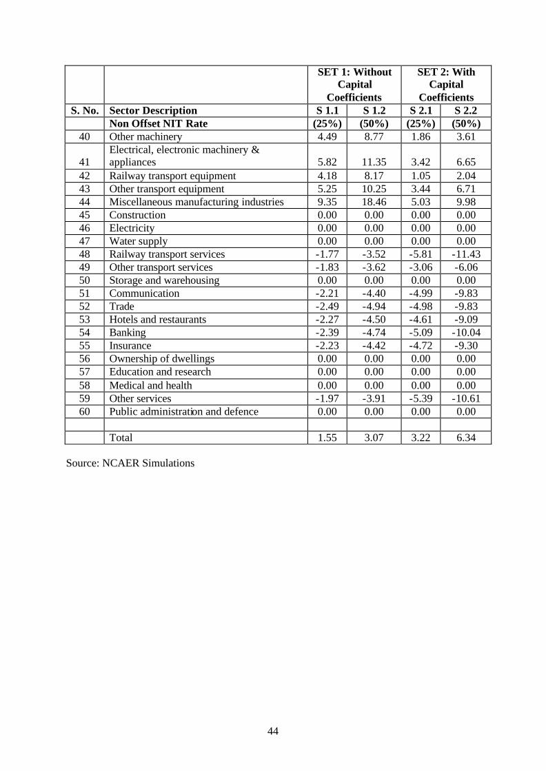
44

SET 1: Without Capital

Coefficients

SET 2: With Capital

Coefficients S. No. Sector Description S 1.1 S 1.2 S 2.1 S 2.2

Non Offset NIT Rate (25%) (50%) (25%) (50%) 40 Other machinery 4.49 8.77 1.86 3.61

41 Electrical, electronic machinery & appliances 5.82 11.35 3.42 6.65

42 Railway transport equipment 4.18 8.17 1.05 2.04 43 Other transport equipment 5.25 10.25 3.44 6.71 44 Miscellaneous manufacturing industries 9.35 18.46 5.03 9.98 45 Construction 0.00 0.00 0.00 0.00 46 Electricity 0.00 0.00 0.00 0.00 47 Water supply 0.00 0.00 0.00 0.00 48 Railway transport services -1.77 -3.52 -5.81 -11.43 49 Other transport services -1.83 -3.62 -3.06 -6.06 50 Storage and warehousing 0.00 0.00 0.00 0.00 51 Communication -2.21 -4.40 -4.99 -9.83 52 Trade -2.49 -4.94 -4.98 -9.83 53 Hotels and restaurants -2.27 -4.50 -4.61 -9.09 54 Banking -2.39 -4.74 -5.09 -10.04 55 Insurance -2.23 -4.42 -4.72 -9.30 56 Ownership of dwellings 0.00 0.00 0.00 0.00 57 Education and research 0.00 0.00 0.00 0.00 58 Medical and health 0.00 0.00 0.00 0.00 59 Other services -1.97 -3.91 -5.39 -10.61 60 Public administration and defence 0.00 0.00 0.00 0.00 Total 1.55 3.07 3.22 6.34

Source: NCAER Simulations

45

Table 9: Percentage Change in Import

SET 1: Without Capital

Coefficients

SET 2: With Capital

Coefficients S. No. Sector Description S 1.1 S 1.2 S 2.1 S 2.2

Non Offset NIT Rate (25%) (50%) (25%) (50%) 1 Food crops 1.97 3.90 5.88 11.57 2 Cash crops 1.91 3.81 7.11 13.98 3 Plantation crops 1.86 3.69 6.40 12.59 4 Other crops 1.94 3.85 6.26 12.31 5 Animal husbandry 2.01 3.98 5.89 11.59 6 Forestry & logging 1.81 3.59 6.34 12.45 7 Fishing 2.31 4.58 4.36 8.60 8 Coal and lignite 2.77 5.48 6.28 12.36 9 Natural gas & Crude Petroleum 1.32 2.60 3.11 6.10 10 Iron ore 2.68 5.30 6.05 11.91 11 Other minerals 0.26 0.49 -3.45 -6.76 12 Sugar 2.43 4.81 3.16 6.24 13 Food products excluding sugar 2.52 5.00 4.43 8.73 14 Beverages 2.48 4.91 -0.41 -0.75 15 Tobacco products 2.48 4.92 5.16 10.17 16 Cotton textiles 2.73 5.35 0.52 1.01 17 Wool, silk & synthetic fibre textiles 0.64 1.23 -5.18 -10.18 18 Jute, hemp and mesta textiles 2.64 5.24 4.31 8.49 19 Textiles products including wearing apparel 2.26 4.23 -13.08 -25.85 20 Wood and wood products except furniture 3.29 6.53 8.28 16.32 21 Furniture and fixture 3.02 6.01 7.57 14.93 22 Paper and paper products 2.00 3.98 3.59 7.10 23 Printing, publishing and allied activities 3.31 6.58 5.75 11.38 24 Leather and leather products 2.67 5.30 8.05 15.85 25 Plastic and rubber products 1.38 2.75 2.49 4.94 26 Petroleum products 1.79 3.56 3.73 7.37 27 Coal tar products 2.77 5.50 3.91 7.74 28 Inorganic heavy chemicals 1.40 2.80 2.07 4.11 29 Organic heavy chemicals -1.11 -2.12 0.25 0.55 30 Fertilizers 1.65 3.28 2.09 4.14 31 Paints, varnishes and lacquers 1.11 2.24 2.39 4.75 32 Pesticides, drugs and other chemicals 1.23 2.47 2.60 5.15 33 Cement 2.04 4.04 3.40 6.71 34 Non metallic mineral products 1.92 3.80 3.23 6.38 35 Iron & steel industries and foundries 1.17 2.34 4.50 8.88 36 Other basic metal industry 0.66 1.34 3.31 6.53

37 Metal products except mach & transport Equipment 1.34 2.68 4.35 8.58

38 Agricultural machinery 2.51 5.01 6.67 13.17 39 Industrial machinery for food and textiles 1.70 3.42 6.48 12.80 40 Other machinery 1.93 3.87 6.77 13.37

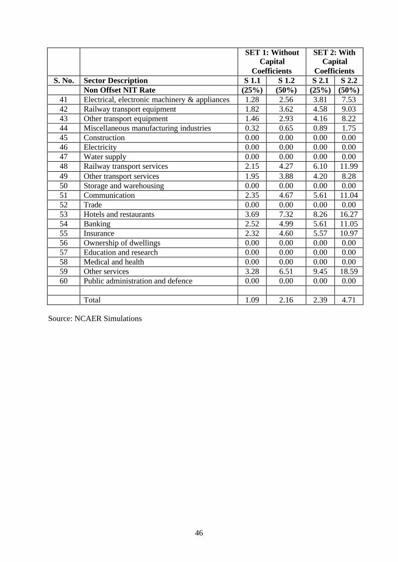
46

SET 1: Without Capital

Coefficients

SET 2: With Capital

Coefficients S. No. Sector Description S 1.1 S 1.2 S 2.1 S 2.2

Non Offset NIT Rate (25%) (50%) (25%) (50%) 41 Electrical, electronic machinery & appliances 1.28 2.56 3.81 7.53 42 Railway transport equipment 1.82 3.62 4.58 9.03 43 Other transport equipment 1.46 2.93 4.16 8.22 44 Miscellaneous manufacturing industries 0.32 0.65 0.89 1.75 45 Construction 0.00 0.00 0.00 0.00 46 Electricity 0.00 0.00 0.00 0.00 47 Water supply 0.00 0.00 0.00 0.00 48 Railway transport services 2.15 4.27 6.10 11.99 49 Other transport services 1.95 3.88 4.20 8.28 50 Storage and warehousing 0.00 0.00 0.00 0.00 51 Communication 2.35 4.67 5.61 11.04 52 Trade 0.00 0.00 0.00 0.00 53 Hotels and restaurants 3.69 7.32 8.26 16.27 54 Banking 2.52 4.99 5.61 11.05 55 Insurance 2.32 4.60 5.57 10.97 56 Ownership of dwellings 0.00 0.00 0.00 0.00 57 Education and research 0.00 0.00 0.00 0.00 58 Medical and health 0.00 0.00 0.00 0.00 59 Other services 3.28 6.51 9.45 18.59 60 Public administration and defence 0.00 0.00 0.00 0.00 Total 1.09 2.16 2.39 4.71

Source: NCAER Simulations

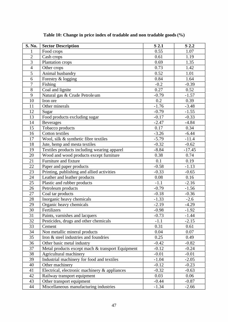
47

Table 10: Change in price index of tradable and non tradable goods (%)

S. No. Sector Description S 2.1 S 2.2

1 Food crops 0.55 1.07 2 Cash crops 0.61 1.19 3 Plantation crops 0.69 1.35 4 Other crops 0.73 1.42 5 Animal husbandry 0.52 1.01 6 Forestry & logging 0.84 1.64 7 Fishing -0.2 -0.39 8 Coal and lignite 0.27 0.52 9 Natural gas & Crude Petroleum -0.79 -1.57 10 Iron ore 0.2 0.39 11 Other minerals -1.76 -3.48 12 Sugar -0.79 -1.55 13 Food products excluding sugar -0.17 -0.33 14 Beverages -2.47 -4.84 15 Tobacco products 0.17 0.34 16 Cotton textiles -3.26 -6.44 17 Wool, silk & synthetic fibre textiles -5.79 -11.4 18 Jute, hemp and mesta textiles -0.32 -0.62 19 Textiles products including wearing apparel -8.84 -17.45 20 Wood and wood products except furniture 0.38 0.74 21 Furniture and fixture 0.1 0.19 22 Paper and paper products -0.58 -1.13 23 Printing, publishing and allied activities -0.33 -0.65 24 Leather and leather products 0.08 0.16 25 Plastic and rubber products -1.1 -2.16 26 Petroleum products -0.79 -1.56 27 Coal tar products -0.18 -0.36 28 Inorganic heavy chemicals -1.33 -2.6 29 Organic heavy chemicals -2.19 -4.29 30 Fertilizers -0.98 -1.92 31 Paints, varnishes and lacquers -0.73 -1.44 32 Pesticides, drugs and other chemicals -1.1 -2.15 33 Cement 0.31 0.61 34 Non metallic mineral products 0.04 0.07 35 Iron & steel industries and foundries 0.25 0.49 36 Other basic metal industry -0.42 -0.82 37 Metal products except mach & transport Equipment -0.12 -0.24 38 Agricultural machinery -0.01 -0.01 39 Industrial machinery for food and textiles -1.04 -2.05 40 Other machinery -0.12 -0.23 41 Electrical, electronic machinery & appliances -0.32 -0.63 42 Railway transport equipment 0.03 0.06 43 Other transport equipment -0.44 -0.87 44 Miscellaneous manufacturing industries -1.34 -2.66

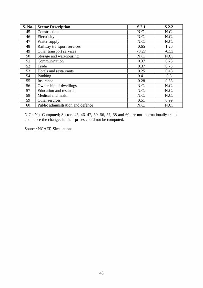
48

S. No. Sector Description S 2.1 S 2.2 45 Construction N.C. N.C. 46 Electricity N.C. N.C. 47 Water supply N.C. N.C. 48 Railway transport services 0.65 1.26 49 Other transport services -0.27 -0.53 50 Storage and warehousing N.C. N.C. 51 Communication 0.37 0.73 52 Trade 0.37 0.73 53 Hotels and restaurants 0.25 0.48 54 Banking 0.41 0.8 55 Insurance 0.28 0.55 56 Ownership of dwellings N.C. N.C. 57 Education and research N.C. N.C. 58 Medical and health N.C. N.C. 59 Other services 0.51 0.99 60 Public administration and defence N.C. N.C.

N.C.: Not Computed; Sectors 45, 46, 47, 50, 56, 57, 58 and 60 are not internationally traded and hence the changes in their prices could not be computed. Source: NCAER Simulations

49

Table 11: Distribution of NIT on Output Across Sectors: Row-wise (Rs. Lakh)

IO Code Description NIT Output

NIT/Q ( per cent)

01 Food crops -2086575 24018772 -8.69 02 Cash crops -682985 8415368 -8.12 03 Plantation crops 24232 6158859 0.39 04 Other crops -727627 14717186 -4.94 05 Animal husbandry 98468 18281531 0.54 06 Forestry & logging 12586 2486237 0.51 07 Fishing -24193 3171641 -0.76 08 Coal and lignite 37849 3504984 1.08 09 Natural gas & Crude Petroleum 1572581 3417653 46.01 10 Iron ore 1182 466676 0.25 11 Other minerals 110803 1362604 8.13 12 Sugar 31884 3347510 0.95 13 Food products excluding sugar 833178 18862942 4.42 14 Beverages 714053 2578789 27.69 15 Tobacco products 737087 1146560 64.29 16 Cotton textiles 375788 5775566 6.51 17 Wool, silk & synthetic fibre textiles 120459 3779899 3.19 18 Jute, hemp and mesta textiles 53213 448282 11.87 19 Textiles products including wearing apparel 281182 8352802 3.37 20 Wood and wood products except furniture 70861 848314 8.35 21 Furniture and fixture 35251 817397 4.31 22 Paper and paper products 518687 2413073 21.49 23 Printing, publishing and allied activities 54543 2093160 2.61 24 Leather and leather products 138497 1633695 8.48 25 Plastic and rubber products 995325 6013370 16.55 26 Petroleum products 3918424 17375676 22.55 27 Coal tar products 99261 829162 11.97 28 Inorganic heavy chemicals 488915 2926687 16.71 29 Organic heavy chemicals 766579 2495675 30.72 30 Fertilizers -1048480 3200493 -32.76 31 Paints, varnishes and lacquers 305084 1762397 17.31 32 Pesticides, drugs and other chemicals 1451577 14640229 9.91 33 Cement 495235 1897034 26.11 34 Non metallic mineral products 652155 4045898 16.12 35 Iron & steel industries and foundries 2313552 13749377 16.83 36 Other basic metal industry 914284 2979788 30.68

37 Metal products except mach & transport Equipment 789777 5798872 13.62

38 Agricultural machinery 51117 1048495 4.88 39 Industrial machinery for food and textiles 100150 823870 12.16 40 Other machinery 1467790 7662699 19.16 41 Electrical, electronic machinery & appliances 2378747 16443198 14.47 42 Railway transport equipment 68935 865713 7.96 43 Other transport equipment 1218135 9216468 13.22

50

IO Code Description NIT Output

NIT/Q ( per cent)

44 Miscellaneous manufacturing industries 1657502 7100046 23.34 45 Construction 870099 44152788 1.97 46 Electricity -1380044 14790883 -9.33 47 Water supply 2846 786315 0.36 48 Railway transport services -251404 5513456 -4.56 49 Other transport services 19809 36359410 0.05 50 Storage and warehousing 936 308332 0.30 51 Communication -123309 5728231 -2.15 52 Trade 0 45422021 0.00 53 Hotels and restaurants 31226 10292468 0.30 54 Banking 50319 16842287 0.30 55 Insurance 12873 4239538 0.30 56 Ownership of dwellings 42300 13931500 0.30 57 Education and research 292959 10887331 2.69 58 Medical and health 223029 7301778 3.05 59 Other services 383179 21413849 1.79 60 Public administration and defence 47414 15615700 0.30 Total 21607300 512560534

Source: NCAER computation based on IO 2003-04.

51

Bibliography

Bird, Richard M. and Michael Smart (2008): “The Impact on Investment of Replacing a Retail Sales Tax by a Value-Added Tax: Evidence from Canadian Experience”, Working Paper No. 15, the Institute of International Business, University of Toronto.

Bird, Richard M. and Pierre-Pascal Gendron (2007): The VAT in Developing and Transition Countries, Cambridge University Press, Cambridge.

Bird, Richard M., Jack M. Mintz and Thomas A. Wilson (2006): “Coordinating Federal and Provincial Sales Taxes” Lessons from Canadian Experience”, National Tax Journal, (59), 809-25

Boesters et al: “Economic Effects of VAT Reform in Germany”, Discussion Paper No. 06-030, ZEW, Centre for European Economic Research.

Brown, Drusilla K., Alan V. Deardorff and Robert M. Stern (1996): “Computational Analysis of the Economic Effects of an East Asian Preferential Trading Bloc”, Journal of the Japanese and International Economies, 10: 37-70.

Brumbaugh (2006): “Taxes and Interna tional Competitiveness”, CRS Report for Congress, Order Code RS22445.

Central Statistical Organisation (2008): “Input-Output Transactions Table 2003-04”, GOI, Ministry of Statistics & Programme Implementation, Central Statistical Organisation, New Delhi.

Central Statistical Organisation (2008): “National Account Statistics”, GOI, Ministry of Statistics & Programme Implementation, Central Statistical Organisation, New Delhi.

Central Statistical Organisation (various years): “Annual Survey of Industries”, GOI, Ministry of Statistics & Programme Implementation, Central Statistical Organisation (Industrial Statistics Wing), Kolkata.

Chadha, Rajesh, Sanjib Pohit, Alan Deardorff and Robert Stern (1998): “The Impact of Trade Policy Reforms: A CGE Modeling Approach”, University of Michigan Press.

Chen and Mintz (2003): “How Canada’s Tax System Discourages Investment”. No. 68, C.D. Howe Institute.

Desai, Mihir A. and James R. Hines (2002): “Value-Added Taxes and International Trade: The Evidence”.

Devarajan et al (1991): “A Value-Added Tax (VAT) in Thailand: Who Wins and Who Loses?”, TDRI Quarterly Review, 6(1).

Dixon, Peter B. and Maureen T. Rimmer (1999): “The Government’s Tax Package: Further Analysis based on Monash Model” General Paper No. G-131, CPSIP, Monash University.

Douette, A. (1973): “The Study of the Capital Coefficient – A Condition of Economic Planning”. Annals of Public and Cooperative Economics, 44(4), pp 345-361, Blackwell Publishers.

Dungan et al (2008): “Growth Oriented Sales Tax Reform for Ontario”, C.D. Howe Institute.

Giesecke and Tran (2009): :Modeling Value Added Tax in the Presence of Multiproduction and Differenciated Exemptions”, General Paper No. G-182, Centre of Policy Studies, Monash University.

52

Govinda Rao, Kumar Sen and R. Jena (2008): “Issues Before the Thirteenth Finance Commission”, Working Paper 2008-55, National Institute of Public Finance and Policy.

Hamilton, Bob and Chun-Yan Kuo (1991): “The Goods and Services Tax: A General Equilibrium Analysis”, Canadian Tax Journal, 39(1).

IMF (2007): “Government Finance Statistics”.

Keen, Michael and Ben Lockwood (2007): “The value-Added Tax: its Causes and Consequences”, Michael Keen & Ben Lockwood, 2007. "The Value Added Tax: Its Causes and Consequences," Economics Working Papers ECO2007/09, European University Institute.

Kelkar (2004): “Implementing FRBM Act, 2003”, Economic and Political Weekly.

Kelkar, Vijay (2009a): “Convocation Address at India Gandhi Institute of Development Research”, IGIDR, Mumbai, 6 February.

Kelkar, Vijay (2009b): Special Address at 3rd National Conference on “GST for Accelerated Economic growth and Competitiveness”, Special Address, New Delhi, 29 June.

Kesselman (2004): “Tax Design for Northern Tiger”, Vol. 10, No. 1, Institute for Research on Public Policy.

Krueger, Anne O. (2008): “The Role of Trade and International Policy in Indian Economic Performance”, Asian Economic Policy Review, (3), Japan Center for Economic Research.

Leontief, Wassily (1953): “Studies in the Structure of the American Economy”, New York - Oxford University Press.

McLure, Charles E. (1998): “Electronic Commerce and the Tax Assignment Problem: Preserving State Sovereignty in a Digital World”, State tax Notes, 14(15), pp 1169-81.

McLure, Charles E. (2003): “Harmonising the RSTs and GST: Lessons from Canada from Canadian Experience”, Hoover Institution, Stanford University.

Meagher, G.A. and Brian R. Parmenter (1993): “Some Short-Run Implications of Fight back: A General Equilibrium Analysis”, General Paper No. G-101, CPSIP, Monash University.

Ministry of Commerce and Industry, Department of Commerce (2008): Office Memorandum: Inputs for 13th Finance Commission, F. No. 19/4/2007 – FT (ST), July 1, 2009.

Ministry of Finance (2008-09): “Indian Public Finance Statistics”, Department of Economic Affairs, Economic Division, GOI.

Ministry of Finance and Company Affairs, GOI (2002): “Report of the Task Force on Indirect Taxes”.

Ministry of Finance, GOI (2004): “Implementation of the Fiscal Responsibility and Budget Management Act, 2003”.

National Sample Survey Organisation (2008): “Unorganised Manufacturing Sector in India: Input, Output and Value Added – NSS 62nd Round (July 2005 – June 2006)”, Ministry of Statistics & Programme Implementation, GOI, Report No. 526(62/2.2/3).

National Sample Survey Organisation (2008): “Unorganised Manufacturing Sector in India: Employment, Assets and Borrowings – NSS 62nd Round (July 2005 – June 2006)”, Ministry of Statistics & Programme Implementation, GOI, Report No. 525(62/2.2/2).

NCAER (2005): “Export Promotion Scheme Replacing DEPB Scheme”.

53

Poddar, Satya and Ehtisham Ahmad (2009): “GST Reforms and Intergovernmental Considerations in India”, Ministry of Finance, Government of India.

Rao, M. Govinda and R. Kavita Rao (2006): “Trends and Issues in Tax Policy and Reform in India”, India Policy Forum – 2005-06, NCAER-Brookings Institution.

Saluja, M. R. (1980): “Component-Wise Capital-Output Ratio in the Indian Economy”, sankhya: The Indian Journal of Statistics’, 42, Series D.

Shankar (2005): “Thirty Years of Tax Reform in India”, Economic and Political Weekly.

Smart and Bird (2006): “The GST Cut and Fiscal Imbalance”, ITP Paper 0604, International tax Programme, Institute for International Business, University of Toronto.

Wytter, Glyn and Kym Anderson (2002): “Impact of the GST and Wine Tax Reform on Australia’s Wine Industry: A CGE Analysis”, Australian Economic Papers, Blackwell Publishing Limited.

54

Annex 1: Capital Coefficients Matrix

In this section we discuss the methodology for compiling capital coefficients matrix for the

Indian economy. An earlier study had worked out capita-output ratios for the Indian economy

for two time periods: 1951-52 to 1961-62 and 1962-63 to 1971-72 (Saluja 1980).

For each of the manufacturing sectors (IO sectors 12 to 44 in our aggregation scheme),

capital formation has been computed as the gross value of actual addition to fixed assets

(Gross Fixed Capital Formation: GFCF) at current prices. This data is available from the

information recorded in Block C on Fixed Assets, of the Annual Survey of Industries (ASI)

(refer Table A1). The ASI data has been obtained from the Central Statistical Organisation

(CSO) in electronic form. The ASI data is available under the National Industrial

Classification scheme (NIC) – 2004 at the 3-digit level. In order to map the NIC codes with

the manufacturing sectors in the IO matrix, a concordance scheme has been designed by us

(Table A2). This mapping has been used to concord the NIC data with the manufacturing

sectors in the IO matrix.

The information on capital formation is available under the following categories:

i) land; ii) building; iii) plant & machinery; iv) transport equipment; v) computer equipment

including software; vi) pollution control equipment; vii) others; and viii) capital work in

progress; and ix) total. These broad categories have been compressed into three groups

referred to as (i) Construction; (ii), Plant & machinery including others (iii + v + vi + vii);

and Transport equipment (iv). Further, for each sector, Total GFCF (excluding land) has

been defined as the sum of these three broad categories.

For manufacturing sectors where only aggregate information is ava ilable from the ASI data,

the same have been apportioned based on the output weights within the group in the IO 2003-

04. For instance, GFCF reported under the NIC 3-digit category 241, has been apportioned

among the IO sectors 28, 29 and 30. Similarly, the GFCF reported under NIC code 242 has

been apportioned among the IO sectors 31and 32; NIC code 273 has been apportioned among

the IO sectors 35 and 36; and NIC code 292 has been apportioned among the IO sectors 38,

39 and 40.

Due to lack of GFCF data for jute, hemp and mesta textiles (IO 18), the same has been

estimated (from the ASI data for each of the six years) based on its output proportions within

the total textile group output (sum of IO sectors 16, 17, 18 and 19) in the IO 2003-04.

55

Further, the GFCF for the remaining textile sectors (IO sectors 16, 17 and 19) have also been

realigned according to their respective shares in the total textile group output of the year

2003-04.

Similarly, GFCF for cement (IO sector 33) has been estimated based on its proportion in the

group output of total non-metallic mineral products (sum of IO sectors 33 and 34). The GFCF

for non-metallic mineral products (IO sector 34) has also been realigned according to its

output-based proportion within in the group.

Thus, we have compiled GFCF (at current prices) in each of the manufacturing sectors of the

economy.8 A time series has been was complied for the six years 1999-00 through 2004-05.

For agriculture, mining and service sectors, the capital formation data has been compiled

from data obtained from the CSO (Table A3). This data is available at current prices. Further,

data on capital formation in the agriculture, mining and service sectors is available only under

two categories namely, building; and plant & machinery. Due to lack of data, capital

formation of transport equipment has been considered zero for the agriculture and service

sectors.

It may be mentioned that the information on capital formation in the agriculture, mining and

service sectors is available for aggregate sectors. These have been apportioned (for all the six

years 1999-00 to 2004-05) among the relevant sectors of the IO matrix based on their

respective proportions in total output during the year 2003-04. Table A4 provides detailed

mapping of the non-manufacturing sectors with relevant IO sectors. For instance, capital in

agriculture during the 1999-00 was apportioned among the IO sectors 01 to 05 according to

their respective shares within the group output (of IO sector 01 to 05) in the IO matrix for the

year 2003-04. The same proportions were applied to capital formation in all the years and all

three types of capital formation.

The GFCF values at current prices have been transformed to corresponding values at constant

1999-2000 prices using the price indices for the respective types of capital computed by using

the data from National Accounts Statistics (NAS), 2008 (Table A5).

Thus, based on the earlier discussion we have obtained the sectoral composition of capital

formation at 1999-00 prices in all three categories namely, construction; plant & machinery;

and transport equipment.

8 Capital formation in sugar (IO 12) has been taken as proxy from the capital formation in food products excluding sugar (IO 13).

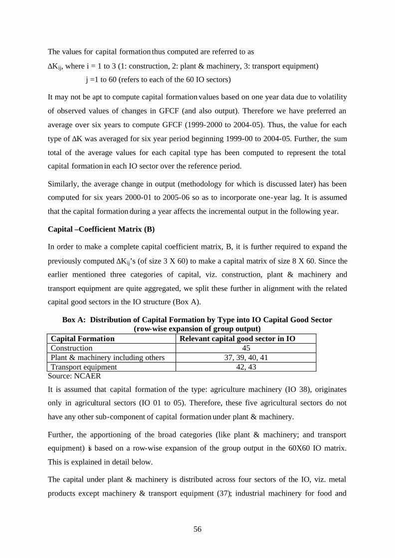
56

The values for capital formation thus computed are referred to as

∆Kij, where i = 1 to 3 (1: construction, 2: plant & machinery, 3: transport equipment)

j =1 to 60 (refers to each of the 60 IO sectors)

It may not be apt to compute capital formation values based on one year data due to volatility

of observed values of changes in GFCF (and also output). Therefore we have preferred an

average over six years to compute GFCF (1999-2000 to 2004-05). Thus, the value for each

type of ∆K was averaged for six year period beginning 1999-00 to 2004-05. Further, the sum

total of the average values for each capital type has been computed to represent the total

capital formation in each IO sector over the reference period.

Similarly, the average change in output (methodology for which is discussed later) has been

computed for six years 2000-01 to 2005-06 so as to incorporate one-year lag. It is assumed

that the capital formation during a year affects the incremental output in the following year.

Capital –Coefficient Matrix (B)

In order to make a complete capital coefficient matrix, B, it is further required to expand the

previously computed ∆Kij’s (of size 3 X 60) to make a capital matrix of size 8 X 60. Since the

earlier mentioned three categories of capital, viz. construction, plant & machinery and

transport equipment are quite aggregated, we split these further in alignment with the related

capital good sectors in the IO structure (Box A).

Box A: Distribution of Capital Formation by Type into IO Capital Good Sector (row-wise expansion of group output)

Capital Formation Relevant capital good sector in IO Construction 45 Plant & machinery including others 37, 39, 40, 41 Transport equipment 42, 43

Source: NCAER

It is assumed that capital formation of the type: agriculture machinery (IO 38), originates

only in agricultural sectors (IO 01 to 05). Therefore, these five agricultural sectors do not

have any other sub-component of capital formation under plant & machinery.

Further, the apportioning of the broad categories (like plant & machinery; and transport

equipment) is based on a row-wise expansion of the group output in the 60X60 IO matrix.

This is explained in detail below.

The capital under plant & machinery is distributed across four sectors of the IO, viz. metal

products except machinery & transport equipment (37); industrial machinery for food and

57

textiles (39); other machinery (40); and electrical, electronic machinery & appliances (41).

The distribution is weighed according to their proportions within the group output in the IO

2003-04 (row-wise expansion of the group output).

Further, we assume that capital formation under industrial machinery for food and textiles

(39) originates only in food products (IO 12-14) and textile products (IO 16-19). The values

have been apportioned by taking respective share in the output of the corresponding group

(column-wise expansion of the group output) (refer Box B).

Box B: Distribution of Plant & Machinery Capital into IO Sectors (column-wise expansion of group output)

Capital origination in IO sector IO sectors for column-

wise expansion Metal products except machinery & transport equipment (37) 06 to 60 Agriculture machinery (38) 01 to 05 Industrial machinery for food and textiles (39) 12 to 14, 16 to 19 Other machinery (40) 06 to 60 Electrical, electronic machinery & appliances (41) 06 to 60

Source: NCAER

The GFCF in transport equipment is distributed across two sectors, viz. railway transport

equipment (IO 42) and other transport equipment (IO 43) with the help of row-wise

expansion of the group output in the IO 2003-04.

The construction capital has been mapped into the IO construction sector (IO 45).

The above methodology provided us with a 8 X 60 ∆K matrix.

Capital Formation at factor cost

Based on the available data, the capital formation in the ∆K matrix thus computed has entries

valued in market prices in contrast to the IO matrix transactions flows measured at factor

cost. It is thus important that before we compute the capital matrix, ∆K should also be at

factor cost.

In order to compute the NIT; and trade & transport proportions, we have first transformed the

IO transaction matrix at factor cost into IO matrix at market prices by adding the NIT (from

the T2 matrix); and trade & transport margin (from TTM matrix. We then compute a share

matrix (of tax; and trade & transport collectively referred to as TTT) with the following

formula:

58

( )ijijij

ijijij TTMNITA

TTMNITTTT

++

+=

where i,j =1 to 60 (refers to each of the 60 IO sectors)

Aij : ijth flow in the IO transaction table

The capital matrix ∆K, was thus adjusted to factor cost using the shares thus computed

The capital formation refers to 8 capitals good sectors, with positive values residing only in

the 8 rows, others being zero. The capital formation matrix B, at factor cost, is obtained by

multiplying the capital coefficient matrix (bij) with the output in IO 2003-04.

Output (Q)

The ASI data on value of output for the manufacturing sectors (sectors 12 to 44 of the IO

matrix) has been extracted for six years beginning 1999-00 up to 2005-06. Since the ASI data

is available at the NIC 3-digit level, the outputs have been concorded to the IO sectors (IO

sectors 12 to 44) (Table A2).

For manufacturing sectors where only aggregate information is available from the ASI data,

the same have been apportioned using the same methodology as adopted for capital

formation. For instance, NIC code 241 has been apportioned among the IO sectors 28, 29 and

30; NIC code 242 among the IO sectors 31and 32; NIC code 273 among the IO sectors 35

and 36; and NIC code 292 among the IO sectors 38, 39 and 40.

In absence of data on value of output for jute, hemp and mesta textiles (IO 18), the same has

been estimated by apportioning the value of output of the total textile group, as done in the

case of estimating the capital formation for the textiles group (refer section on capital

formation for details). Also, the output of remaining textile sectors (IO sectors 16, 17 and 19)

have been adjusted accordingly.

The same exercise has been done in order to estimate the value of output for cement (IO

sector 33) from the group output of total non-metallic mineral products (sum of IO sectors 33

and 34).

Also, it may be observed that value of output for sugar (IO 12) is not available in the ASI

data. A time series for the sugar output has been generated by applying annual growth rates

of sugarcane output (which have been computed from data in the NAS, 2008) on the sugar

output in the IO 2003-04.

59

The value of output at current prices has been converted into 1999-00 constant prices with the

help of price indices computed from the NAS, 2008 (refer Table A6).

The output data (i.e. value of output) for the remaining sectors, i.e. agriculture & allied;

mining; and services is sourced from the NAS, 2008 at 1999-00 constant prices. However, for

some non-manufacturing sectors, data on value of output was not available. In such cases, we

arrived at an approximation by multiplying the sectoral GDP (that was available from NAS at

constant prices) with the output-to-GVA ratio of that sector in the IO matrix of the year 2003-

04. The underlying assumption here being that the ratio of output to value added remains

unchanged over the years. Such IO sectors included electricity (IO 46), water supply (IO 47),

other transport services (IO 49), storage and warehousing (IO 50), trade (IO 52), hotels and

restaurants (IO 53), banking (IO 54), insurance (IO 55), education and research (IO 57),

medical and health (IO 58) and other services (IO 59).

In the case of mining sectors (IO 08, 09, 10 and 11) for which only aggregated data are

available, the same have been apportioned based on the output proportions in the

corresponding group in the IO 2003-04.

The incremental output in each year was computed as the difference between output (in that

year) and that of the preceding year. This is referred to as ∆Q.

Thus we have computed

∆Qik, where i =1 to 60 (refers to each of the IO sectors)

k = 2000-01 to 2005-06

An average ∆Q was obtained by averaging over the six year values. It is referred to as ∆Qi

where i =1 to 60.

It may be mentioned that the negative values of ∆Qi (decline in output) have been ignored for

the purpose of taking averages. These included sectors namely food crops (IO 01), sugar (IO

12), tobacco (IO 15) and plastics (IO 25).

Capital to Output ratio (∆K by ∆Q)

The above mentioned ∆K matrix at factor cost is a 60 x 60 matrix representing the capital

formation in a flow form (Table A7). This is converted into coefficients by dividing with the

output (i.e. average ∆Q) of respective IO sector. Thus, we arrive at the capital-coefficient

60

matrix, “bij”. This is essentially a matrix of size 8 X 60, with the coefficients being zero in

rows corresponding to the non-capital good sectors (Table A8).9

9 The capital coefficients computed in this Annex refer to the registered / organized sectors of the economy. However, the IOTT (2003-04) matrix covers the entire economy: registered as well as unregistered. It is worthwhile to compute capital coefficients for unregistered manufacturing sectors as well. The data for aggregate capital formation and aggregate output for unregistered manufacturing are available from National Accounts Statistics (NAS) 2008. However, this document does not provide sectoral details of capital formation. The aggregate incremental capital-output ratio turns out to be 1.36 for the registered manufacturing. The corresponding value is 1.46 for the unregistered manufacturing sector. The data on capital formation for unregistered sector of manufacturing provided by NAS (2008) can not be compared with that of the “Unorganised Manufacturing Sector in India: Employment, Asserts and Borrowings”, NSSO (2005-06). The difference is huge seems to arise due to difference in methods of computing capital formation.

61

Table A1: Annual Survey of Industries BLOCK C: FIXED ASSETS DSL No./PSL No………

Gross Value (Rs.) Depreciation (Rs.) Net Value (Rs.) Addition during the year

Sl. No.

Types of Assets Opening

as on ----

Due to revaluation

Actual Addition

Deduction & Adjustment during the year

Closing as on ---- (3+4+5-6)

Up to year beginning

Provid-ed during the year

Up to year end (8+9)

Opening as on ----- (3-8)

Closing as on ------ (7-10)

(1) (2) (3) (4) (5) (6) (7) (8) (9) (10) (11) (12) 1. Land

2. Building 3. Plant &Machinery 4. Transport equipment 5. Computer equipment

including software

6. Pollution Control Equipment

7. Others 8. Sub-total (2 to 7) 9. Capital work in

progress

10. Total (1+8+9)

Source: ASI

62

Table A2: Concordance between NIC 3-digit (2004) and IO 60 Sectors

S.No. IO 60 Code

NIC code Description

1 05 014 Agricultural and animal husbandry service activities, except veterinary activities 2 11 142 Mining and quarrying, n.e.c. 3 11 233 Processing of nuclear fuels 4 13 151 Production, processing and preservation of meat, fish, fruit vegetables, oils and fats 5 13 152 Manufacture of dairy products 6 13 153 Manufacture of grain mill products, starches and starch products, and prepared animal feeds 7 13 154 Manufacture of other food products 8 14 155 Manufacture of beverages 9 15 160 Manufacture of tobacco products 10 16 171 Spinning, weaving and finishing of textiles 11 17 243 Manufacture of man-made fibers 12 19 172 Manufacture of other textiles 13 19 173 Manufacture of knitted and crocheted fabrics and articles 14 19 181 Manufacture of wearing apparel, except fur apparel 15 19 182 Dressing and dyeing of fur; manufacture of articles of fur 16 20 201 Saw milling and planing of wood 17 20 202 Manufacture of products of wood, cork, straw and plaiting materials 18 21 361 Manufacture of furniture 19 22 210 Manufacture of paper and paper product 20 23 221 Publishing 21 23 222 Printing and service activities related to printing 22 24 191 Tanning and dressing of leather, manufacture of luggage, handbags, saddlery and harness 23 24 192 Manufacture of footwear 24 25 251 Manufacture of rubber products 25 25 252 Manufacture of plastic products 26 26 232 Manufacture of refined petroleum products 27 27 231 Manufacture of coke oven products 28 28, 29, 30 241 Manufacture of basic chemicals

63

S.No. IO 60 Code

NIC code Description

29 31, 32 242 Manufacture of other chemical products 30 34 261 Manufacture of glass and glass products 31 34 269 Manufacture of non-metallic mineral products n.e.c. 32 35 271 Manufacture of Basic Iron & Steel 33 35, 36 273 Casting of metals 34 36 272 Manufacture of basic precious and non-ferrous metals 35 37 281 Manufacture of structural metal products, tanks, reservoirs and steam generators 36 37 289 Manufacture of other fabricated metal products; metal working service activities 37 37 293 Manufacture of domestic appliances, n.e.c. 38 38, 39, 40 292 Manufacture of special purpose machinery 39 40 291 Manufacture of general purpose machinery 40 41 300 Manufacture of office, accounting and computing machinery 41 41 311 Manufacture of electric motors, generators and transformers 42 41 313 Manufacture of insulated wire and cable 43 41 314 Manufacture of accumulators, primary cells and primary batteries 44 41 315 Manufacture of electric lamps and lighting equipment 45 41 319 Manufacture of other electrical equipment n.e.c. 46 41 321 Manufacture of electronic valves and tubes and other electronic components 47 41 322 Manufacture of television and radio transmitters and apparatus for line telephony and line telegraphy

48 41 323 Manufacture of television and radio receivers, sound or video recording or reproducing apparatus, and associated goods

49 42 352 Manufacture of railway and tramway locomotives and rolling stock 50 43 341 Manufacture of motor vehicles 51 43 342 Manufacture of bodies (coach work) for motor vehicles; manufacture of trailers and semi- trailers 52 43 343 Manufacture of parts and accessories for motor vehicles and their engines 53 43 351 Building and repair of ships & boats 54 43 359 Manufacture of transport equipment n.e.c.

55 44 331 Manufacture of medical appliances and instruments and appliances for measuring, checking, testing, navigating and other purposes except optical instruments

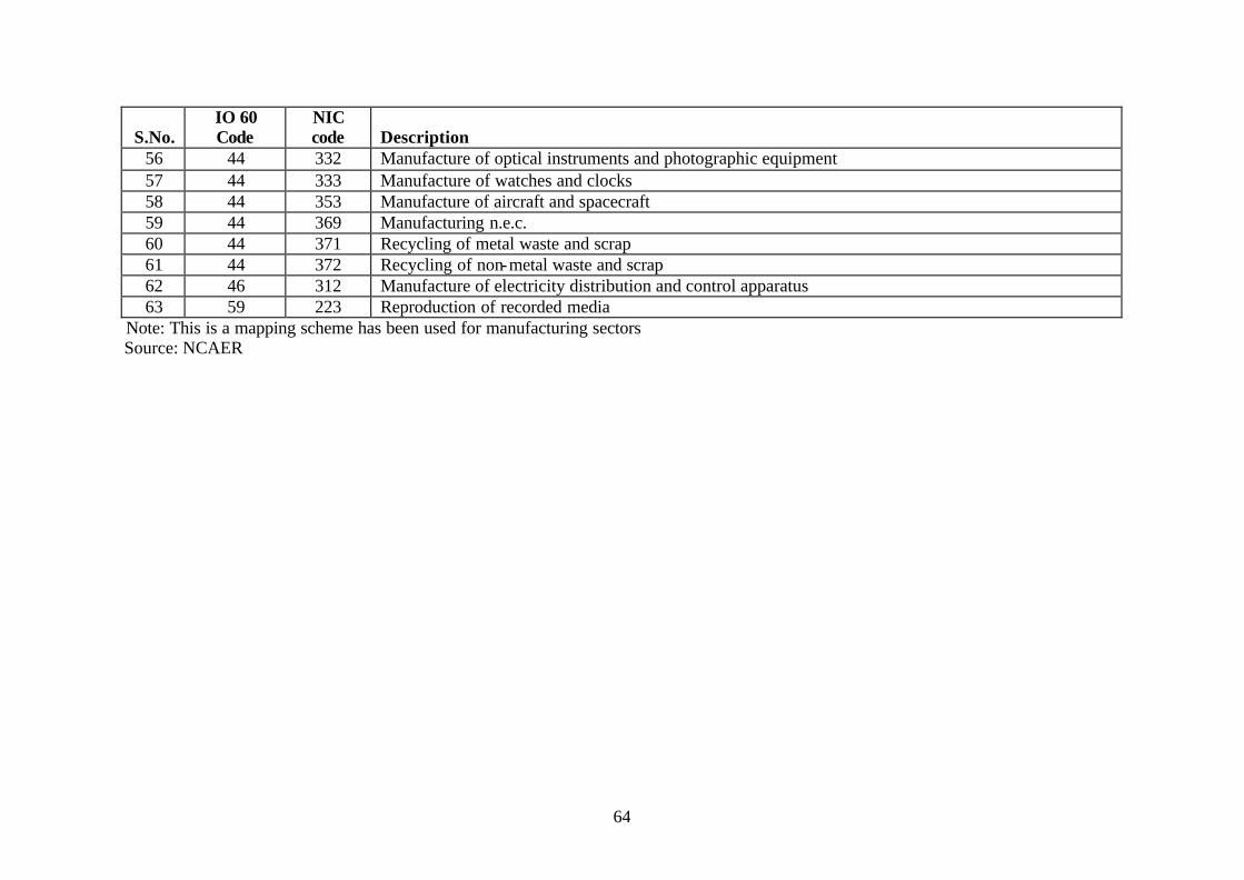
64

S.No. IO 60 Code

NIC code Description

56 44 332 Manufacture of optical instruments and photographic equipment 57 44 333 Manufacture of watches and clocks 58 44 353 Manufacture of aircraft and spacecraft 59 44 369 Manufacturing n.e.c. 60 44 371 Recycling of metal waste and scrap 61 44 372 Recycling of non-metal waste and scrap 62 46 312 Manufacture of electricity distribution and control apparatus 63 59 223 Reproduction of recorded media

Note: This is a mapping scheme has been used for manufacturing sectors Source: NCAER

65

Table A3: GFCF by type of assets at current prices (Rs. Crore) S.N. Industry 1999-2000 2000-01 Construction Machinery Total Construction Machinery Total 1 agriculture, forestry & fishing 24921 21454 46375 23189 21605 44793 1.1 agriculture 23950 15773 39724 22172 15913 38085 1.2 forestry & logging 971 53 1024 1017 32 1049 1.3 fishing -1 5628 5627 -1 5660 5658 2 mining & quarrying 4392 5602 9994 4067 3402 7469 3 manufacturing 45465 99403 144869 49829 96494 146323 3.1 registered 23511 82820 106331 22011 75486 97497 3.2 unregistered 21954 16583 38537 27817 21008 48826 4 elect. gas & water supply 18174 20605 38780 20842 20206 41048 5 construction 1817 7096 8913 1320 7084 8404 6 Trade, hotels & restaurants 4328 7235 11564 5099 7727 12827 6.1 trade 3035 5579 8610 2951 5056 8000 6.2 hotels & restaurants 1292 1657 2954 2148 2671 4827 7 Transport, storage & communication 17041 41406 58448 21833 54147 75980 7.1 railways 3730 1391 5121 3881 1597 5479 7.2 transport by other means 4434 31661 36097 4640 40613 45253 7.3 storage 228 21 248 300 22 322 7.4 communication 8650 8332 16982 13011 11915 24927 8 financing, insurance, real estate & business services 76984 6780 83764 75624 8271 83896 8.1 banking & insurance 2308 4923 7231 1573 5309 6882 8.2 real estate, ownership of dwellings & business services 74676 1857 76533 74051 2962 77014 9 community, social & personal services 42722 10988 53709 44878 12197 57077 9.1 public administration & defence 29416 4999 34415 31069 6010 37079 9.2 other services 13306 5988 19294 13809 6188 19998 10 Total 235844 220569 456416 246681 231135 477818

66

S.N. Industry 2001-02 2002-03 1 agriculture, forestry & fishing Construction Machinery Total Construction Machinery Total 1.1 agriculture 30052 29471 59523 27512 31692 59203 1.2 forestry & logging 28851 20966 49817 26559 22832 49391 1.3 fishing 1201 26 1227 952 43 994 2 mining & quarrying 0 8479 8479 0 8817 8818 3 manufacturing 6140 3643 9783 4706 4621 9328 3.1 registered 39597 87367 126963 53806 104360 158167 3.2 unregistered 22197 74216 96413 23076 81154 104231 4 elect. gas & water supply 17399 13151 30550 30730 23206 53937 5 construction 22550 24341 46891 24778 19563 44341 6 Trade, hotels & restaurants 4837 10051 14888 6503 11018 17520 6.1 trade 7597 12356 19955 5306 9436 14742 6.2 hotels & restaurants 5202 9401 14603 3864 7595 11456 7 Transport, storage & communication 2395 2954 5352 1442 1840 3286 7.1 railways 19713 43465 63175 19321 60125 79445 7.2 transport by other means 5167 1684 6851 6364 2717 9081 7.3 storage 3336 29438 32771 5089 46257 51346 7.4 communication 483 46 529 492 42 534 8 financing, insurance, real estate & business services 10727 12298 23024 7375 11110 18484 8.1 banking & insurance 112506 8555 121062 111097 5678 116774 8.2 real estate, ownership of dwellings & business services 2811 5573 8384 1247 2714 3961 9 community, social & personal services 109695 2982 112678 109850 2964 112814 9.1 public administration & defence 59224 16716 75938 67157 18331 85490 9.2 other services 38713 7757 46470 43559 8336 51895 10 Total 20510 8959 29468 23598 9995 33595

67

S.N. Industry 2003-04 2004-05

Construction Machinery Total Construction Machinery Total 1 agriculture, forestry & fishing 29753 28962 58715 35060 33979 69038 1.1 agriculture 28057 20799 48856 34163 24353 58516 1.2 forestry & logging 1696 35 1731 896 121 1016 1.3 fishing 0 8128 8128 0 9505 9505 2 mining & quarrying 11921 3480 15401 12242 15864 28106 3 manufacturing 75476 137403 212879 119924 220816 340741 3.1 registered 29072 102372 131444 47972 166506 214479 3.2 unregistered 46404 35032 81435 71952 54310 126262 4 elect. gas & water supply 24390 32866 57256 27010 30031 57041 5 construction 9797 11124 20922 8961 13896 22856 6 Trade, hotels & restaurants 11049 18921 29972 13568 22819 36387 6.1 trade 8378 15632 24010 9440 17794 27231 6.2 hotels & restaurants 2671 3289 5962 4128 5025 9156 7 Transport, storage & communication 18665 60594 79258 20522 78853 99375 7.1 railways 8012 2688 10700 9764 3211 12975 7.2 transport by other means 5370 51919 57289 6786 64684 71470 7.3 storage 509 24 533 453 25 478 7.4 communication 4774 5962 10736 3519 10932 14452 8 financing, insurance, real estate & business services 111667 9606 121272 109929 11656 121586 8.1 banking & insurance 1811 4328 6139 1831 4064 5895 8.2 real estate, ownership of dwellings & business services 109855 5278 115133 108098 7593 115691 9 community, social & personal services 72515 19700 92215 94360 26491 120850 9.1 public administration & defence 44811 8143 52954 55043 10983 66026 9.2 other services 27704 11557 39261 39317 15508 54824 10 Total 365233 322654 687890 441576 454405 895980

68

S.N. Industry 2005-06 2006-07 1 agriculture, forestry & fishing Construction Machinery Total Construction Machinery Total 1.1 agriculture 41289 39770 81058 48601 45974 94575 1.2 forestry & logging 40068 29093 69161 47023 34159 81182 1.3 fishing 1221 69 1290 1578 66 1644 2 mining & quarrying 0 10607 10608 0 11749 11749 3 manufacturing 14302 10419 24721 9176 15033 24208 3.1 registered 146749 289697 436447 188128 365112 553241 3.2 unregistered 69212 231157 300369 88145 289621 377766 4 elect. gas & water supply 77537 58540 136077 99983 75492 175475 5 construction 38013 41395 79409 46393 52262 98654 6 Trade, hotels & restaurants 8210 18350 26561 14766 20308 35074 6.1 trade 13209 22511 35719 17833 30795 48630 6.2 hotels & restaurants 9002 17299 26298 13210 24978 38188 7 Transport, storage & communication 4207 5212 9421 4623 5816 10443 7.1 railways 18848 132238 151085 21605 154329 175934 7.2 transport by other means 9778 5268 15045 12275 5855 18129 7.3 storage 5673 60872 66546 6643 68227 74870 7.4 communication 511 38 548 532 86 618 8 financing, insurance, real estate & business services 2887 66060 68946 2155 80161 82317 8.1 banking & insurance 132958 18542 151499 140145 21409 161554 8.2 real estate, ownership of dwellings & business services 2609 5345 7954 4065 7254 11319 9 community, social & personal services 130348 13197 143545 136080 14156 150235 9.1 public administration & defence 103088 23014 126102 124669 27304 151974 9.2 other services 75436 11604 87040 91290 13460 104750 10 Total 27652 11410 39062 33379 13844 47223

69

S.N. Industry 2007-08 1 agriculture, forestry & fishing Construction Machinery Total 1.1 agriculture 58688 50333 109021 1.2 forestry & logging 57018 37711 94729 1.3 fishing 1670 73 1743 2 mining & quarrying 0 12549 12549 3 manufacturing 12167 19849 32017 3.1 registered 214837 431356 646193 3.2 unregistered 104799 348248 453047 4 elect. gas & water supply 110038 83108 193146 5 construction 54224 56856 111080 6 Trade, hotels & restaurants 17040 22853 39893 6.1 trade 15949 27347 43297 6.2 hotels & restaurants 10160 19976 30136 7 Transport, storage & communication 5789 7371 13161 7.1 railways 28493 205451 233945 7.2 transport by other means 16080 7618 23699 7.3 storage 9439 102059 111498 7.4 communication 481 36 517 8 financing, insurance, real estate & business services 2493 95738 98231 8.1 banking & insurance 175442 21629 197070 8.2 real estate, ownership of dwellings & business services 4935 8913 13848 9 community, social & personal services 170507 12715 183223 9.1 public administration & defence 159611 33312 192922 9.2 other services 119094 15693 134787 10 Total 40517 17619 58135

70

Table A4: Mapping of the Non-Manufacturing Sectors with relevant IO sectors

Industry IO and ASI Codes

Agriculture, forestry & fishing

Agriculture IO: 01 ,02, 03, 04 05 (from ASI: 014)

Forestry & logging IO: 06

Fishing IO: 07

Mining & quarrying IO: 08, 09, 10 11 (from ASI: 142,233)

Services

Elect. gas & water supply IO: 46, 47

Construction IO: 45

Trade, hotels & restaurants

Trade IO: 52

Hotels & restaurants IO: 53

Transport, storage & communication

Railways IO: 48

71

Industry IO and ASI Codes

Transport by other means IO: 49

Storage IO: 50

Communication IO: 51

Financing, insurance, real estate & business services

Banking & insurance IO: 54, 55

Real estate, ownership of dwellings & business services IO: 56

Education & Research IO: 57 (from ASI (NIC 731)

Medical and health (IO 58) same as in ownership of dwellings (56)

Community, social & personal services

Public administration & defence IO: 60

Other services IO: 59

Source: NCAER

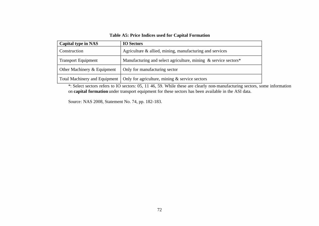
72

Table A5: Price Indices used for Capital Formation

Capital type in NAS IO Sectors

Construction Agriculture & allied, mining, manufacturing and services

Transport Equipment Manufacturing and select agriculture, mining & service sectors*

Other Machinery & Equipment Only for manufacturing sector

Total Machinery and Equipment Only for agriculture, mining & service sectors

*: Select sectors refers to IO sectors: 05, 11 46, 59. While these are clearly non-manufacturing sectors, some information on capital formation under transport equipment for these sectors has been available in the ASI data. Source: NAS 2008, Statement No. 74, pp. 182-183.

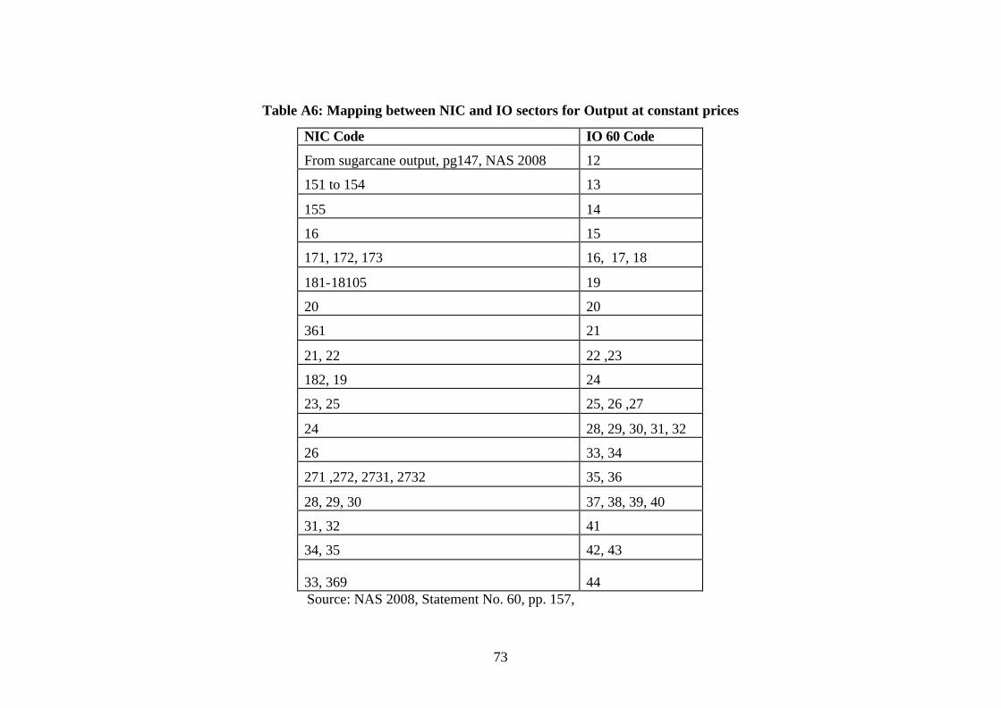
73

Table A6: Mapping between NIC and IO sectors for Output at constant prices

NIC Code IO 60 Code

From sugarcane output, pg147, NAS 2008 12

151 to 154 13

155 14

16 15

171, 172, 173 16, 17, 18

181-18105 19

20 20

361 21

21, 22 22 ,23

182, 19 24

23, 25 25, 26 ,27

24 28, 29, 30, 31, 32

26 33, 34

271 ,272, 2731, 2732 35, 36

28, 29, 30 37, 38, 39, 40

31, 32 41

34, 35 42, 43

33, 369 44 Source: NAS 2008, Statement No. 60, pp. 157,

74

Table A7: Average Values of Capital Formation and Change in Output (Rs. Lakh)

IO Code Description 1 2 3 4 5 6 7 8 9 10

37 Metal products except mach & transport Equipment - - - - - 682 101980 37391 34609 5057

38 Agricultural machinery 608827 217305 159872 441611 2168 - - - -

39 Industrial machinery for food and textiles - - - - - - - - -

40 Other machinery - - - - - 925 147125 51835 50333 6890

41 Electrical, electronic machinery & appliances - - - - - 1844 - 106689 108308 15838

42 Railway transport equipment - - - 43 Other transport equipment - - - - - - - - - - 45 Construction 1067962 374170 273858 654381 1995 98365 (24) 290706 283452 38713

Change in Q 1572500 630900 217680 597640 129487 31850 80633 122895 119833 16363

IO Code Description 11 12 13 14 15 16 17 18 19 20

37 Metal products except mach & transport Equipment

63 45347 42051 24344 3958 25052 16885 1807 34685 893

38 Agricultural machinery - - - - - - - - - -

39 Industrial machinery for food and textiles

- 30538 172637 23594 - 51336 34573 3930 77448 -

40 Other machinery 84 56916 59972 34112 5385 32088 22277 2641 47386 1226

41 Electrical, electronic machinery & appliances

196 123960 133287 76975 - 75099 48139 5832 98533 2815

42 Railway transport equipment 9 1923 - - - 50 939 110 43 Other transport equipment 81 18557 16536 6794 1566 5814 4109 487 9126 1001 45 Construction 104 64777 66800 35443 6433 26189 17140 2032 37875 1716

Change in Q 47777 96554 680728 38631 87901 216861 141928 16832 313576 46750

75

IO Code Description 21 22 23 24 25 26 27 28 29 30

37 Metal products except mach & transport Equipment

764 17658 7905 3339 26045 123205 4541 26609 22003 30163

38 Agricultural machinery - - - - - - - - - -

39 Industrial machinery for food and textiles

- - - - - - - - - -

40 Other machinery 1047 23069 11175 4453 34689 163109 5680 36264 30135 37191

41 Electrical, electronic machinery & appliances

2296 53188 22233 10512 77977 381328 12918 76879 65175 79641

42 Railway transport equipment 64 412 332 285 704 163 69 189 162 206 43 Other transport equipment 619 4017 2875 2775 6883 1590 - 1961 1473 1999 45 Construction 2143 14549 8662 6249 18418 33128 1014 11903 10151 13017

Change in Q 45474 107257 86740 96409 197507 1460760 10729 109885 93702 120166

IO Code Description 31 32 33 34 35 36 37 38 39 40

37 Metal products except mach & transport Equipment

5316 43235 13389 27050 90739 19700 12532 2164 1629 15539

38 Agricultural machinery - - - - - - - - - -

39 Industrial machinery for food and textiles

- - - - - - - - - -

40 Other machinery 6812 54738 17752 37416 126212 26661 17891 2956 2328 21496

41 Electrical, electronic machinery & appliances

15102 121143 38098 83218 280885 60127 38828 6776 4594 46896

42 Railway transport equipment 158 1293 - 611 1304 282 871 130 105 951 43 Other transport equipment 1438 12948 - 5966 12999 2787 8579 1212 1017 9181 45 Construction 7472 62069 10422 22226 60694 13153 14843 2555 2007 18669

Change in Q 48913 406317 45071 96125 795183 162079 294928 17971 14121 411202

76

IO Code Description 41 42 43 44 45 46 47 48 49 50

37 Metal products except mach & transport Equipment

38453 395 55249 8141 133224 320605 16501 27897 523195 401

38 Agricultural machinery - - - - - - -

39 Industrial machinery for food and textiles

- - - - - - -

40 Other machinery 53174 541 83862 11085 180776 422371 22488 39899 789976 545

41 Electrical, electronic machinery & appliances

114163 1130 177802 23348 418342 858409 47036 88990 1656078 1150

42 Railway transport equipment 659 31 1460 642 - - - - 43 Other transport equipment 6477 317 13670 5330 - - - - - - 45 Construction 27024 597 39486 13587 484535 1895000 100743 523879 427865 35502

Change in Q 615543 19088 1318153 306150 4219317 517735 20498 270783 2486149 8025

IO Code Description

51 52 53 54 55 56 57 58 59 60 Total Capital

Formation

37 Metal products except mach & transport Equipment

135503 121732 38267 48425 12189 17 51627 126929 - 2527078

38 Agricultural machinery - - - 1429784

39 Industrial machinery for food and textiles

- - - 394056

40 Other machinery 183781 188825 52015 65665 16530 23 69996 174628 - 3536455

41 Electrical, electronic machinery & appliances

446053 430273 109906 137143 34591 50 145542 377138 - 7342474

42 Railway transport equipment - - - 14114 43 Other transport equipment - - - - - 5 - - - 170188 45 Construction 723877 463027 199747 136172 34278 8489442 0 8489456 1955437 - 27715088

Change in Q 523317 2873509 774164 898978 282239 275817 564332 567876 1740700 - 28110227 Note: Capital Formation is averaged over 1999-2000 to 2004-05, Change in Output is averaged for years 2000-01 to 2005-06 Source: NCAER computations

77

Table A8: Capital Coefficient Matrix IO 60 Code

Description 01 02 03 04 05 06 07 08 09 10 11 12 13 14 15

37 Metal products except mach & Tpt Equipment

0.0000 0.0000 0.0000 0.0000 0.0000 0.0214 1.2647 0.3043 0.2888 0.3091 0.0013 0.4697 0.0618 0.6302 0.0450

38 Agricultural machinery 0.3872 0.3444 0.7344 0.7389 0.0167 0.0000 0.0000 0.0000 0.0000 0.0000 0.0000 0.0000 0.0000 0.0000 0.0000

39 Industrial machinery for food and textiles

0.0000 0.0000 0.0000 0.0000 0.0000 0.0000 0.0000 0.0000 0.0000 0.0000 0.0000 0.3163 0.2536 0.6107 0.0000

40 Other machinery 0.0000 0.0000 0.0000 0.0000 0.0000 0.0290 1.8246 0.4218 0.4200 0.4210 0.0018 0.5895 0.0881 0.8830 0.0613

41 Electrical, electronic machinery & appliances

0.0000 0.0000 0.0000 0.0000 0.0000 0.0579 0.0000 0.8681 0.9038 0.9679 0.0041 1.2838 0.1958 1.9926 0.0000

42 Railway transport equipment 0.0000 0.0000 0.0000 0.0000 0.0000 0.0000 0.0000 0.0000 0.0000 0.0000 0.0002 0.0000 0.0028 0.0000 0.0000

43 Other transport equipment 0.0000 0.0000 0.0000 0.0000 0.0000 0.0000 0.0000 0.0000 0.0000 0.0000 0.0017 0.1922 0.0243 0.1759 0.0178

45 Miscellaneous manufacturing industries

0.0000 0.0000 0.0000 0.0000 0.0000 0.0000 0.0000 0.0000 0.0000 0.0000 0.0000 0.0000 0.0000 0.0000 0.0000

Construction 0.6791 0.5931 1.2581 1.0949 0.0154 3.0884 -0.0003 2.3655 2.3654 2.3659 0.0022 0.6709 0.0981 0.9175 0.0732

IO 60 Code Description 16 17 18 19 20 21 22 23 24 25 26 27 28 29 30 37 Metal products except mach &

Tpt Equipment 0.1155 0.1190 0.1073 0.1106 0.0191 0.0168 0.1646 0.0911 0.0346 0.1319 0.0843 0.4233 0.2422 0.2348 0.2510

38 Agricultural machinery 0.0000 0.0000 0.0000 0.0000 0.0000 0.0000 0.0000 0.0000 0.0000 0.0000 0.0000 0.0000 0.0000 0.0000 0.0000

39 Industrial machinery for food and text iles

0.2367 0.2436 0.2335 0.2470 0.0000 0.0000 0.0000 0.0000 0.0000 0.0000 0.0000 0.0000 0.0000 0.0000 0.0000

40 Other machinery 0.1480 0.1570 0.1569 0.1511 0.0262 0.0230 0.2151 0.1288 0.0462 0.1756 0.1117 0.5294 0.3300 0.3216 0.3095

41 Electrical, electronic machinery & appliances

0.3463 0.3392 0.3465 0.3142 0.0602 0.0505 0.4959 0.2563 0.1090 0.3948 0.2610 1.2041 0.6996 0.6956 0.6628

42 Railway transport equipment 0.0000 0.0000 0.0030 0.0030 0.0024 0.0014 0.0038 0.0038 0.0030 0.0036 0.0001 0.0065 0.0017 0.0017 0.0017

43 Other transport equipment 0.0268 0.0290 0.0289 0.0291 0.0214 0.0136 0.0375 0.0331 0.0288 0.0348 0.0011 0.0000 0.0178 0.0157 0.0166

44 Miscellaneous manufacturing industries 0.0000 0.0000 0.0000 0.0000 0.0000 0.0000 0.0000 0.0000 0.0000 0.0000 0.0000 0.0000 0.0000 0.0000 0.0000

45 Construction 0.1208 0.1208 0.1207 0.1208 0.0367 0.0471 0.1356 0.0999 0.0648 0.0933 0.0227 0.0945 0.1083 0.1083 0.1083

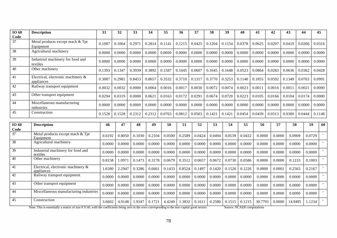
78

IO 60 Code

Description 31 32 33 34 35 36 37 38 39 40 41 42 43 44 45

37 Metal products except mach & Tpt Equipment

0.1087 0.1064 0.2971 0.2814 0.1141 0.1215 0.0425 0.1204 0.1154 0.0378 0.0625 0.0207 0.0419 0.0266 0.0316

38 Agricultural machinery 0.0000 0.0000 0.0000 0.0000 0.0000 0.0000 0.0000 0.0000 0.0000 0.0000 0.0000 0.0000 0.0000 0.0000 0.0000

39 Industrial machinery for food and textiles

0.0000 0.0000 0.0000 0.0000 0.0000 0.0000 0.0000 0.0000 0.0000 0.0000 0.0000 0.0000 0.0000 0.0000 0.0000

40 Other machinery 0.1393 0.1347 0.3939 0.3892 0.1587 0.1645 0.0607 0.1645 0.1648 0.0523 0.0864 0.0283 0.0636 0.0362 0.0428

41 Electrical, electronic machinery & appliances

0.3087 0.2981 0.8453 0.8657 0.3532 0.3710 0.1317 0.3770 0.3253 0.1140 0.1855 0.0592 0.1349 0.0763 0.0991

42 Railway transport equipment 0.0032 0.0032 0.0000 0.0064 0.0016 0.0017 0.0030 0.0072 0.0074 0.0023 0.0011 0.0016 0.0011 0.0021 0.0000

43 Other transport equipment 0.0294 0.0319 0.0000 0.0621 0.0163 0.0172 0.0291 0.0674 0.0720 0.0223 0.0105 0.0166 0.0104 0.0174 0.0000

44 Miscellaneous manufacturing industries

0.0000 0.0000 0.0000 0.0000 0.0000 0.0000 0.0000 0.0000 0.0000 0.0000 0.0000 0.0000 0.0000 0.0000 0.0000

45 Construction 0.1528 0.1528 0.2312 0.2312 0.0763 0.0812 0.0503 0.1421 0.1421 0.0454 0.0439 0.0313 0.0300 0.0444 0.1148

IO 60 Code

Description 46 47 48 49 50 51 52 53 54 55 56 57 58 59 60

37 Metal products except mach & Tpt Equipment 0.6192 0.8050 0.1030 0.2104 0.0500 0.2589 0.0424 0.0494 0.0539 0.0432 0.0000 0.0000 0.0909 0.0729 -

38 Agricultural machinery 0.0000 0.0000 0.0000 0.0000 0.0000 0.0000 0.0000 0.0000 0.0000 0.0000 0.0000 0.0000 0.0000 0.0000 -

39 Industrial machinery for food and textiles 0.0000 0.0000 0.0000 0.0000 0.0000 0.0000 0.0000 0.0000 0.0000 0.0000 0.0000 0.0000 0.0000 0.0000 -

40 Other machinery 0.8158 1.0971 0.1473 0.3178 0.0679 0.3512 0.0657 0.0672 0.0730 0.0586 0.0000 0.0000 0.1233 0.1003 -

41 Electrical, electronic machinery & appliances 1.6580 2.2947 0.3286 0.6661 0.1433 0.8524 0.1497 0.1420 0.1526 0.1226 0.0000 0.0001 0.2563 0.2167 -

42 Railway transport equipment 0.0000 0.0000 0.0000 0.0000 0.0000 0.0000 0.0000 0.0000 0.0000 0.0000 0.0000 0.0000 0.0000 0.0000 -

43 Other transport equipment 0.0000 0.0000 0.0000 0.0000 0.0000 0.0000 0.0000 0.0000 0.0000 0.0000 0.0000 0.0000 0.0000 0.0000 -

44 Miscellaneous manufacturing industries 0.0000 0.0000 0.0000 0.0000 0.0000 0.0000 0.0000 0.0000 0.0000 0.0000 0.0000 0.0000 0.0000 0.0000 -

45 Construction 3.6602 4.9148 1.9347 0.1721 4.4240 1.3832 0.1611 0.2580 0.1515 0.1215 30.7793 0.0000 14.9495 1.1234 -

Note: This is essentially a matrix of size 8 X 60, with the coefficients being zero in the rows corresponding to the non-capital good sectors Source: NCAER computations