impact of multi-altimeter sea level assimilation in the ... of multi-altimeter sea level...
TRANSCRIPT

1
Impact of Multi-altimeter Sea Level Assimilation in the Mediterranean Forecasting Model
M.-I. Pujol(1), S. Dobricic(2), N. Pinardi(3), M. Adani(2)
(1) Istituto Nazionale di Geofisica e Vulcanologia, Gruppo di Oceanografia Operativa, via A. Moro 44, 40128 Bologna, Italy (2) Centro Euro-Mediterraneo per i Cambiamenti Climatici, via A. Moro 44, 40128 Bologna, Italy (3) Alma Mater Studiorum Università di Bologna, Centro Interdipartimentale per la Ricerca sulle Scienze Ambientali, Via S. Alberto 163, 48100 Ravenna, Italy Correspondence to: M.-I. Pujol CLS-DOS 8-10 rue Hermes, Parc Technologique du canal 31520 Ramonville Saint-Agne, France E-mail : [email protected]

2
Abstract
In this paper we analyze the impact of multi-satellite altimeter observations assimilation in a
high-resolution Mediterranean model. Four different altimeter missions (Jason-1, Envisat,
Topex/Poseidon interleaved and Geosat Follow-On) are used over a 7-month period [September
2004, March 2005] to study the impact of the assimilation of one to four satellites on the analyses
quality. The study highlights three important results. First, it shows the positive impact of the
altimeter data on the analyses. The corrected fields capture missing structures of the circulation and
eddies are modified in shape, position and intensity with respect to the model simulation. Secondly,
the study demonstrates the improvement in the analyses induced by each satellite. The impact of the
addition of a second satellite is almost equivalent to the improvement given by the introduction of
the first satellite: the second satellite data brings a 12% reduction of the root mean square of the
differences between analyses and observations for the Sea Level Anomaly (SLA). The third and
fourth satellite also significantly improve the rms, with more than 3% reduction for each of them.
Finally, it is shown that Envisat and Geosat Follow-On additions to J1 impact the analyses more
than the addition of Topex/Poseidon suggesting that the across track spatial resolution is still one of
the important aspects of a multi-mission satellite observing system. This result could support the
concept of multi-mission altimetric monitoring done by complementary horizontal resolution
satellite orbits.

3
1. Introduction
During the recent decades numerical model simulations have considerably contributed to a
new understanding of the ocean circulation and its variability. Model simulations have become
more realistic and allow the exploration of the synoptic scales of the ocean circulation in a way that
could never be achieved with sparse in-situ measurements. The realism of the model outputs can be
strongly improved by data assimilation of in situ and satellite data. In particular the altimeter data
are key observations to correct the model since they have almost uniform and regular coverage with
a high revisit time period (De Mey and Robinson, 1987; Fukumori et al., 1999, Dobricic et al.
2006).
Since the beginning of altimetry, the question of the optimal spatial and temporal coverage of
satellites in view of assimilation into numerical models has been studied. Mellor an Ezer (1991)
showed that low altimeter spatial sampling could increase the rms error of about 2-3 times with
respect to a finer sampling. Moreover, they showed that error associated with imperfect altimeter
coverage is larger than the error associated with imperfect parameterization of surface to subsurface
correlation unvolved in assimilation technique. However, in a single satellite assimilation context,
spatial and temporal sampling could not be dissociated. .Berry and Marshall (1989) showed that an
altimeter with a 14-day repeat period (with a 140km track separation in the studied area) gave
optimal results. However, as shown by Holland and Malanotte-Rizzoli (1989), when assimilating
along altimeter tracks, the tradeoff between space and time resolution just about compensate for
each other. As underlined by the same authors, the results depends on the assimilation technique
and parameterizations and also on space and time scales of motion in the region studied and
capacity of the model to reproduce these structures and variability.
Since 1992 multi-altimetry data are available (Le Traon, 2002) and numerical models have
increased the spatial resolution reaching few kilometers horizontal grid spacing and the question of

4
the optimal altimeter sampling scheme in an model assimilation context can be reviewed. Recent
studies (Benkiran, 2007) focused on the question of the optimal spatial and temporal coverage of
the satellite in view of the assimilation in numerical models. Benkiran (2007) made a first
estimation of the impact of assimilation of four satellites into an oceanographic data analysis system
of the Northern Atlantic and he found that the impact of the addition of a fourth satellite was
insignificant. However, his result was obtained by a coarse spatial resolution model set-up (1/3°)
and the weekly assimilation window.
In this study we will estimate the impact of the multi-mission spatial/temporal coverage on
the analyses of the Mediterranean Forecasting System (MFS) (Pinardi et al., 2003, 2009). The
numerical model has a resolution of 1/16 x 1/16 degrees of latitude and longitude (approx. 6.5km)
and it is able to represent eddies since the first Rossby radius of deformation is 10 km. Eddies in the
Mediterranean are pervasive (Millot 1999; Millot et Taupier-Letage, 2005; Robinson et al., 2004)
and the reproduction of mesoscales in the sea surface variability is a key parameter to judge the
quality of the assimilation and model system. Furthermore, we will assess the optimal satellite
multi-mission monitoring parameters by estimating how each of four satellites, characterized with
different sampling schemes, impacts the analysis quality.
The study is focused on the period September 2004 to March 2005 during which four different
altimeters were active. Different assimilation experiments for the various altimeter combinations are
shown. They are described in Section 2 after a brief presentation of the MFS model and the
assimilation method used. The high resolution error covariance matrix used for this study is
presented in Section 3. Analysis fields are compared with SLA and ARGO independent data to
estimate the quality of the analyses. The results obtained are discussed in Section 4 in terms of
improvement of the root mean square error for SLA, temperature and salinity. Section 5
summarizes and offers the conclusions.
5
2. Data and Methods
a. The MFS model and its assimilation scheme
The MFS model is based on the OPA8.2 (Océan Parallélisé) code (Madec et al., 1998) with
an implicit free surface. One of the interesting characteristics of this model is its high horizontal and
vertical resolution: it reaches a 1/16°×1/16° horizontal resolution (i.e., approximately 6.5 km) and
72 vertical levels unevenly spaced in order to increase the resolution near the surface. A detailed
description of the model is given in Tonani et al. (2008).
In order to assimilate observations, the MFS model is combined with a three-dimensional
variational assimilation scheme (OceanVar, Dobricic and Pinardi, 2008; Appendix). For this study,
both SST and altimeter data were assimilated. The SST assimilation is done correcting the surface
heat fluxes as explained in Pinardi et al. (2003) by a term proportional to the difference between the
model temperature at the surface and the observational SST. The latter is produced daily by an
objective analysis scheme developed by Buongiorno-Nardelli et al. (2003).
In the OceanVar scheme, the background error covariance is subdivided into a sequence of
operators (Dobricic and Pinardi, 2008), one of them containing statistically estimated vertical error
covariances of temperature and salinity, a key element for the assimilation of SLA observations as
explained in Dobricic et al. (2007). They are represented by multivariate Empirical Orthogonal
Functions (EOFs) computed from a 9-year model simulation (from 1993 to 2001). New EOFs were
computed specifically for this study. The method and the resulting EOFs are presented in the
Section 3.
Assimilation can be used for various purposes (Robinson et Lermusiaux, 2001; Lermusiaux et al.,
2006). In this paper the data assimilation system is used to correct the model background (or first
guess) fields by combining them with the information from observations. In order to do so it is
necessary to make sure that the observed and background quantities are comparable. The altimeter

6
measurements are given as SLA obtained by subtracting a long term mean of the satellite data, the
so-called Mean Sea Surface Height (MSSH), for the period 1993-1999. In order to compute the
model SLA, a Mean Dynamic Topography (MDT) is removed from the model sea surface height.
This MDT was estimated from model output and data for the same period that characterizes the
MSSH (Rio et al., 2007), and further corrected by long term assimilation diagnostics (Dobricic
2005).
The altimeter SLA signal gives the time-dependent dynamical part of the sea level variations
(frequencies higher than 0.05 days-1 have been removed. They correspond to barotropic aliased
signals (Carrère and al., 2003)) which contain a multiplicity of time scales. A major part of the SLA
signal is induced by long time scale signals such as the steric effect (seasonal variability of water
masses) and another part is due to mean currents variability (seasonal to interannual variability) and
shorter time variability mainly dominated by mesoscale structures (< 200 km)..
In the model, the sea surface is a prognostic variable. It represents the dynamic height induced by
large scale forcing of the circulation (wind, water and heat fluxes) and by the mesoscales. Since the
model is incompressible and Boussinesq, the steric contribution to sea level averaged over the
whole model domain does not contribute to the dynamics (Mellor and Ezer, 1995) and should be
excluded from the model-data misfit as already explained in Demirov et al. (2003). As our model
domain is closed we must remove the steric effect from the observations. We remove it by
subtracting the mean of the misfits along each satellite track. The amplitude of the steric oscillation
in the Mediterranean is similar to the North Atlantic where it is about 10-20 cm (Ivchenko et al.
2007, Oddo et al., 2009). The ocean thermal expansion is slow and therefore can be easily estimated
by calculating the basin average SLA once a week. However, there are other large scale effects that
are not simulated by the model and have shorter time scales. For example the inverse barometer is
removed from SLA observations by using the ECMWF atmospheric pressure analyses that contain
some uncertainty. Furthermore, as the only connection to the global ocean is through the narrow
7
strait of Gibraltar, rapidly moving atmospheric pressure disturbances produce barotropic
oscillations that may affect for several days the sea level in the Mediterranean (Le Traon and
Gauzelin 1997). The local variability of the wind in the Gibraltar Strait, poorly represented in the
ECMWF wind analyses, may produce high frequency oscillations of the mean sea level in the
Mediterranean (Fukumori et al. 2006). The intercalibration (Le Traon and Ogor 1998) of satellite
tracks sea level removes most of high frequency barotropic oscillations from the observations, but it
could leave some biased high frequency oscillations at smaller spatial scales. In the MFS
operational system it was found that by removing the mean misfit along each track (Dobricic et al.,
2005) the rms error for SLA was reduced by about 10-20% with respect to the subtraction of the
climatological estimate of the steric height (Demirov et al., 2003).
In this paper we follow this nomenclature: is the analysis state vector containing all the
grid point values of temperature, salinity and sea level, is the background or first guess
model field we want to improve with assimilation and is the observational quantity. The
assimilation scheme computes misfits, or differences between the observations and the model first
guess before the analysis. The analyses correct not only the sea level but also other model state
variables, in particular temperature and salinity vertical profiles through the vertical and horizontal
components of the background error covariances (Dobricic and Pinardi, 2008).
The assimilation cycle is daily and the correction of the model fields is done in filter mode
(Demirov et al , 2003), i.e., only observations in the past are used to produce an analysis. Every day,
up to 600 SLA data points for that day are assimilated along different tracks in the Mediterranean
Sea. It should be mentioned that AVISO (reference?) provides composed gridded data sets that can
be successfully assimilated into ocean models (e.g. Oey et al. 2005). AVISO gridded product is
however weekly and shorter frequencies are ‘averaged’ in the gridding process (AVISO uses a three
weeks temporal window). The key difference between the two approaches (using along track data
and objectively analyzed sea surface height maps) is the fact that using directly along-track

8
altimeter data we allow for the high frequency signal to be assimilated. Although our approach
requires a more careful pre-processing of the along track data, it is more general and does not
preclude the inclusion of all space and time frequencies of the observations in the assimilation
scheme.
The resulting analyses for sea level, η , temperature, T, and salinity, S, are compared after
assimilation to the observations in order to estimate a difference vector, D, defined as:
(1)
where is a simple bilinear interpolation to the observational spatial and temporal point and is
the analysis state vector. These differences are an estimate of the agreement of the analysis with
observations. The mean of the vector values of D and the square root of the mean of will be
called bias and root mean square (rms) of the posterior residuals (or Analyses minus Observations,
hereafter mentioned as AMO) respectively. For SLA differences, the mean is subtracted along each
track, as done for the misfits, in order to eliminate the steric effect. For SLA in particular we
calculated the mean of the absolute value of AMO.
b. The altimeter data
The altimeter data used in this study are along-track, near-real time data distributed by AVISO.
Data from four altimeters were collected: Jason (J1), Topex/Poseidon (TP), Envisat (EN) and
Geosat Follow On (G2). They were geophysically corrected (tides, wet and dry tropospheric,
ionospheric corrections). Low frequency inverse barometer effect and high frequency barotropic
response to wind and pressure forcing given by MOG2D (Modèle aux Ondes de Gravité 2-
Dimensions; Carrere and Lyard, 2003) model was removed to altimeter signal. This allowed an
improved correction of aliasing effect induced by the satellite repetitivity of the measurement. All

9
the data were intercalibrated performing a global crossover adjustment using J1 as reference
mission (Le Traon and Ogor, 1998). Along-track data were re-sampled every 7 km using cubic
splines. SLA were computed removing a 7-year mean sea surface height corresponding to the
period [1993-1999]. Finally, measurement noise was reduced applying Lanczos (cut-off wavelength
of 42 km) and median (21 km) filters. The data were them sub-sampled every ~14km in order to
limit the number of redundant observations.
The characteristics of the different altimeter sampling schemes are given in Table 1. J1 and TP
present the best temporal revisit time but have low spatial resolution. Note that TP tracks are
located at the J1 inter-tracks during the tandem mission (September 2002 – October 2005).
Combination of J1 and TP thus allows an optimal spatial coverage. However, the combination with
temporal coverage is limited since the two satellites are flying side by side. Contrary to J1, EN
presents the higher spatial coverage but longer revisit period. G2 characteristics are halfway
between J1 and EN.
c. Independent data for validation
Argo data are now a consistent real time input data for assimilation and validation in the
Mediterranean Sea (Poulain et al., 2007). Near 700 vertical profiles were collected during the
studied period. The position of the different Argo profiles used is shown in Figure 1. In this study,
Argo data are used a first time as assimilated data set in order to verify the robustness of the
background error covariance matrix (Section 3). In a second instance, Argo profiles are used as an
independent data set (section 4). All statistics computed for AMO by equation (1) with Xa at day J
consider observations at day J+1. In this way we ensure that there is a small overlap between the
analysis fields and the observations used for the error estimate and that errors due to one day
mismatch are much smaller than the corresponding errors in our analyses.

10
SST and color data are used for a qualitative validation of the posterior ocean estimates. These data
are used as gridded maps which are 10-day averages built from MODIS level 2 products
downloaded from the Ocean Color Web (http://oceancolor.gsfc.nasa.gov). They are compared with
the SSH model output.
d. The numerical experiments
Five experiments are illustrated in this paper. They are done in order to analyze the impact of
different background error covariance matrix and to test various satellite combinations and their
impact on the analysis quality. Each experiment covers the period from September 2004 to March
2005. The only difference between experiments is the number of altimeter data assimilated and the
optional assimilation of Argo and XBT profiles.
The different combinations of satellites used in the experiments are summarized in Table 2. The
reference experiment does not assimilate altimeter data (Exp0). In Exp1, only J1 data are
assimilated. Then, two dual-satellite combinations are tested in Exp2a and Exp2b. In the first one
(Exp2a) we consider the combination J1+EN, combining thereby the respective high temporal and
spatial sampling characteristics of each satellite. In Exp2b, the duo J1+TP interleaved is used,
supposedly offering the optimal coverage (Chelton and Schlax, 2003). In Exp3 data from J1, EN
and TP are combined. Finally in Exp4 data from the four satellites (J1, EN, TP and G2) are
assimilated.
An additional experiment (Exp4TS), assimilating four altimeters as well as Argo (T/S) and XBT
profiles, is carried out to analyze the impact of different background error covariance matrices.
An SST relaxation was applied for all the experiments.

11
3. Computation of the background vertical error covariance matrix
Data assimilation requires the knowledge of the spatial/temporal structure of the background
error covariances. In OceanVar (see Appendix) the background error covariances of temperature
and salinity are estimated successively in vertical and horizontal directions. SLA error covariances
are then estimated as the steady state solution of a barotropic oceanographic model simulation
forced by temperature and salinity error covariances. The accuracy of the analyses of T and S thus
strongly depends on the quality of the estimated covariances of temperature and salinity in the
vertical direction. In Dobricic and Pinardi (2008) vertical error covariances between temperature
and salinity are statistically estimated with vertical Empirical Orthogonal Functions-EOF defined
for 13 regions of the Mediterranean Sea and seasonal temporal resolution. We will mention them as
low-resolution EOF (LR EOF) for they low spatial and temporal resolution. Here we describe the
methodology used to compute higher resolution EOFs that should better fit the model resolution
and its capability to represent smaller spatial scales. We will also show the importance of such part
of the error covariance matrix for the quality of temperature and salinity corrections.
The multivariate vertical error covariance EOFs are estimated considering the covariance matrix
between temperature, salinity and sea level, as described in Dobricic et al. (2005). The matrix
scaling is described in detail in Dobricic et al. (2005) and here we will say only that we considered a
depth constant variance and the geometrical scaling. This was shown to be necessary in order to
maintain the largest scaled errors in the thermocline. A 9-year [1993, 2001] simulation is used to
define the vertical error covariance matrix and to compute new multivariate vertical EOFs
(hereafter indicated as HR EOFs for their higher spatial and temporal resolution with respect to LR
EOF). The model domain is subdivided into 1/4°x1/4° boxes and for each of them vertical monthly
EOFs are computed. Each box overlaps by an area of 3/4°x3/4° and considers 6 weeks data around

12
the central time of each month. This was done to ensure a smooth transition from an area/month to
the other. Inside each box, only grid points deeper than 500 m were selected so that EOF where
calculated, as well as assimilation was carried out, for depths greater than 500 m. The maximum
number of data available at each grid depth was used to define the maximum depth (Zmax) for each
area and EOFs.
Performances of these new vertical EOFs are estimated in terms of analysis error reduction over the
period September 2004 - March 2005. In order to detect the improvements due to the higher spatial
resolution of EOFs, Exp4 and Exp4TS experiments using HR EOFs and LR EOFs are compared
with available observations. Mean absolute value of bias and rms of AMO for SSH and temperature
and salinity profiles are used to estimate the quality of the analyses.
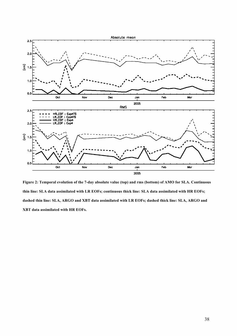
Figure 2 presents the temporal evolution of the 7-day mean of the absolute value of the bias and the
rms of AMO when HR EOFs or LR EOFs are used. The results clearly show a net reduction of the
mean absolute value when HR EOFs are used with respect to the results obtained with LR EOFs.
The reduction of the mean absolute value of the bias and its variance is given in Table 3 in terms of
the percentage of the signal. HR EOFs allows a reduction of more than 61% of the mean absolute
value of the bias and 45% of the rms with respect to the LR EOFs when only SLA data are
assimilated. The introduction of Argo and XBT data leads to a lower reduction of the SLA bias and
rms (45% and 33% respectively, see Table 3). This is probably due to the fact that temperature and
salinity corrections inferred from SLA misfits are not entirely consistent with their corrections
calculated from misfits of Argo and XBT. However, it should be noticed that the mean absolute
value of the bias and the rms of AMO do not represent a reliable measure for the quality of the
analyses, because SLA observations are assimilated. They only show the level of the agreement
between the analyses and the observations. For example a higher agreement represented by lower
rms of AMO may simply reflect higher background error variances for the sea level. All

13
experiments give the mean absolute value of the bias and the rms of AMO which is within the
estimated error of observations of 2-3cm (Ducet et al, 2000; Menard et al., 2003). Therefore the two
sets of EOFs give equally probable analyses of the SLA with or without the addition of XBT and
ARGO profiles.
Performances of HR_EOFs were also analysed by the evaluation of bias and rms of AMO for
temperature and salinity profiles using Argo observations. AMO are calculated a posteriori, as
discussed in section 2.c by spatially interpolating the temperature and salinity analyses on day J to
observational points on day J+1 and by subtracting the observed values on day J+1. Results are
presented in Figure 3 and Figure 4 for temperature and salinity profiles respectively. The reduction
of the bias and the rms of AMO (in terms of % of the Exp0 signal) in the upper 400m is reported in
Table 4.
Assimilation of SLA observations (Exp4) tends to increase the bias of temperature AMO with
respect to the model without the assimilation (Exp0) (Figure 3a; Table 4). Spatial resolution of the
background vertical error covariances has a low impact but overall lower bias is obtained when
HR_EOFs are used, especially in the upper 300m. The bias of AMO for temperature is
approximately 20% smaller when HR_EOFs are used instead of LR_EOFs. The rms of AMO for
Exp4 with both HR_EOF and LR_EOF is impacted by the bias observed (Figure 3b; Table 4). Rms
is actually about 8 to 4.5% higher than for Exp0. However, the analysis of variability of AMO
shows a reduction of about 2 to 3% (respectively for LF_EOFs and HR_EOFs). Overall, the
different EOFs have a small impact on the quality of the analyses in term of AMO variability and
they produce a larger bias when only SLA data are assimilated.
When Argo and XBT profiles are assimilated in addition to SLA data (Exp4TS), the bias and rms of
AMO temperature is largely reduced for both LR_EOF and HR_EOF, and HR_EOF leads to a near
20% higher reduction of the bias than when LR_EOF are used (Figure 3a; Table 4). In the same

14
way, the rms of AMO temperature is significantly reduced reaching 23% and 27.5% of the Exp0
signal for HR_EOF and LR_EOF (Figure 3b; Table 4).
Considering salinity now, Exp4 improves with respect to Exp0 (Figure 4). A significant reduction
of the bias and the rms of AMO salinity is observed especially in the upper 300 m. Best results are
obtained when HR_EOF are used. In this case, salinity bias reduction in Exp4 reaches up to 22% of
the signal and rms is reduced up to 19% with respect to Exp0 (Table 4). When Argo and XBT data
are also assimilated, the results are again largely improved, with slightly higher performances for
LF_EOFs. In this case, AMO salinity bias reduction reaches 70% and 72% of the Exp0 signal for
HR_EOFs and LR_EOFs respectively. The AMO rms reduction is 47% and 49% for HR_EOFs and
LR_EOFs going from Exp0 to Exp4TS.
The results obtained underline the limits and the accuracy of the data assimilation scheme used in
this study. As said before, Fig. 3 and 4 show that the temperature bias and rms error in Exp4 is
larger than Exp0 and the result is not sensitive to the different EOF sets used. The degradation of
the bias and rms is however small, of the order of 0.2 C and this sets the accuracy of our method for
correcting temperature. In the past, assimilation of satellite altimeter data (Ezer and Mellor, 1994,
Masina et al., 2001, Haines, 2002) has been carried out with simpler methods and improvement
between assimilation and no-assimilation experiments has been noticeably positive even if ARGO
data were not available for a quantitative comparison. The models used in the past studies were
however much less skilled in reproducing the ocean variability and an estimate of the accuracy limit
of the assimilation scheme was not possible. In our case it seems that such limit can be set at few
tens of a degree for temperature. For salinity the EXP0 error is much larger from the start and the
assimilation overall improves.
In conclusion, we believe the assimilation skill is improved by using HR_EOFs with respect to
LR_EOF. Even if the benefit is more evident in the case of assimilation of both SLA and
temperature and salinity profiles, we will use the HR_EOF in all the remaining experiments.

15
4. Impact of number of altimeters on analysis quality
a. Impact of number of altimeters on SLA analyses
The impact of the different satellite combinations on the quality of the analyzed SLA is estimated
by computing AMO using (1), as done previously for temperature and salinity analysis. Considering
results presented in chapter 3, experiments were performed by using HR_EOFs. AMO is calculated
for SLA observations by all four satellites. Those differences are calculated a posteriori, by spatially
interpolating the SLA analyses on day J to observational points on day J+1 and by subtracting the
observed values on day J+1. This may be done by assuming that mesoscale fields are highly
correlated from one day to the other. Independent data validation will be done only for temperature
and salinity profiles.
The temporal evolution of AMO rms for SLA is presented in Figure 5. The difference was
computed globally along all satellites tracks and for each altimeter independently in order to
underline the impact of each altimeter. It is clear that the rms of AMO for SLA is reduced by
assimilating all satellites. The assimilation of four satellites (Exp4) gave best results with a mean
rms of AMO of ∼4 cm, i.e., almost the rms error of the altimeter measurement (Ducet et al, 2000;
Menard et al., 2003), whereas when using J1 data only (Exp1), the rms is almost 5 cm. Without
assimilation of SLA (Exp0) the rms is almost 6 cm.
The reduction of the rms of AMO for SLA, expressed in % of the signal between an experiment and
the other, is given in Table 5. The rms steadily decreases with the addition of satellites. It is
interesting to note in Table 5 that the impact of EN is slightly higher than the impact of TP when
added to J1. Considering EN as the second satellite with J1 (Exp2a) the reduction of the rms is
almost 15% and up to 17% along G2 tracks. In the same way, considering TP as the second satellite
(Exp2b) a global reduction of near 12% is obtained (13% along G2 tracks).

16
In a statistical reconstruction study, Chelton and Schlax (2003) showed that SLA mapping
capabilities are improved when combining J1 and TP rather than J1 and EN. However, our results
obtained by assimilating SLA observations with a high resolution numerical model differ from
those obtained by the simpler statistical algorithms. For a high-resolution model, it seems more
beneficial to assimilate high across-track spatial resolution data (like EN data) in addition to J1
rather than additional high temporal resolution data (like TP). This result is confirmed by Exp3 and
Exp4. In addition, we see that the impact from the addition of G2 is higher than that from the
addition of TP (especially along J1 and EN tracks), even if G2 is used as a fourth satellite.
Moreover, the limit of the spatial coverage of TP and J1 is underlined by the negative result
obtained with Exp3 when looking at the signal along the J1 tracks: instead of reducing the rms of
AMO, the assimilation of TP data induced a small increase of the error. This is certainly because TP
tracks are exactly on the J1 inter-track. As a consequence, considering the 10 km Rossby radius of
deformation in the Mediterranean Sea, the correction given by TP is not propagated – or hardly – on
J1 tracks.
In most cases the representation of the mesoscales is optimal when 4 altimeters are used. The spatial
distribution of the reduction of the mean rms of AMO (over the studied period) from an experiment
to another is given in Figure 6. The energetic areas (i.e. Ierapetra area, central Ionian and Algerian
basin, evidenced by Pujol et Larnicol, 2006) are clearly impacted from Exp0 to Exp1. The reduction
of the rms of AMO reaches up to 30% in these areas. However, while a decrease of rms is observed
in most of the points (global mean reduction of 13% of the rms), in some points it is increasing (up
to 20%). The increase of errors going from Exp0 to Exp1 is probably due to the non-uniform
sampling scheme of J1 by itself while in the case of two and three satellites the problem is
alleviated even if consistency between the raw signals of the satellites becomes an issue. In our case
we use inter-calibrated along track products which should have the most compatible signals
between satellites. In any case, our work concentrates on the basin and time mean average values of
17
the errors due to the addition of different satellites and specific work on sub-areas should be done in
the future.
The second satellite reduces the most the rms in points where there is the largest increase by first
satellite. This indicates that the second satellite is complementary to the first, especially at the
intertrack location of this last one. The impact of the insertion of a second to a fourth altimeter is to
refine position, shape and intensity of various eddies, especially in the areas of important mesoscale
variability (Algerian basin, Ionian basin, Levantine Sea). Note that in term of reduction of the rms
of the AMO, the impact of the second satellite (Exp2a and/or Exp2b) is almost as important as the
contribution of the first satellite (Exp1). In fact, the mean rms reduction over the Mediterranean Sea
is nearly 12% for EN (Exp2a) and nearly 10% for TP (Exp2b). It locally reaches nearly 30% (in the
Levantine Sea). The impact of the third and fourth satellites in term of rms reduction is lower: a
reduction of around 3% is observed in Exp3 and Exp4. However, using a third and fourth satellite
largely contributes to the precision of the analysis improving representation of position, intensity
and shape of predicted eddies.
The impact of the SLA assimilation can be also estimated by the surface Eddy Kinetic Energy
(EKE) of the analyses, as shown in Table 6. The assimilation of the first satellite (Exp1) induced an
increase of the mean EKE of 27% with respect to the run with no assimilation (Exp0). However, the
impact in terms of EKE of the assimilation of a second, third or fourth satellite is different.
Assimilation of EN (Exp2a) or TP (Exp2b) as second satellites respectively leads to a 5% and 6%
decrease of the EKE with respect to the one-satellite assimilated run (Exp1). With a third satellite
assimilated (Exp3), an additional decrease of nearly 2% is registered. Finally, adding a fourth
satellite (Exp4) leads to a 2% increase of the mean EKE with respect to Exp3. The mean EKE level
for January 2005 captured by the model corrected with 4-satellites is nearly 200 cm²/s².
This behavior is quite different from that reported by Pascual et al. (2007) from altimetry
reconstructed SLA with 1 and 4 satellites. The mapped products showed a regular increase of the
18
EKE from one to four satellites: +40%, +10% and +5% when two, three and four satellites are
merged. These differences make evident that, assimilating SLA data in a high-resolution model, the
introduction of mesoscale eddies does not automatically impact EKE because the corrections have
to be dynamically adjusted by the model. Given a model horizontal and vertical resolution, the
insertion of new structures in the sea level could modify only available potential energy and some
others will be dissipated by the model representation of viscosity and diffusion. The impact on EKE
of sea level assimilation is connected to the dynamical adjustment by the model of the corrections
while in statistical reconstructions the addition of observations in areas of data-voids automatically
increases the kinetic energy of the flow field but the result is probably dynamically unbalanced.
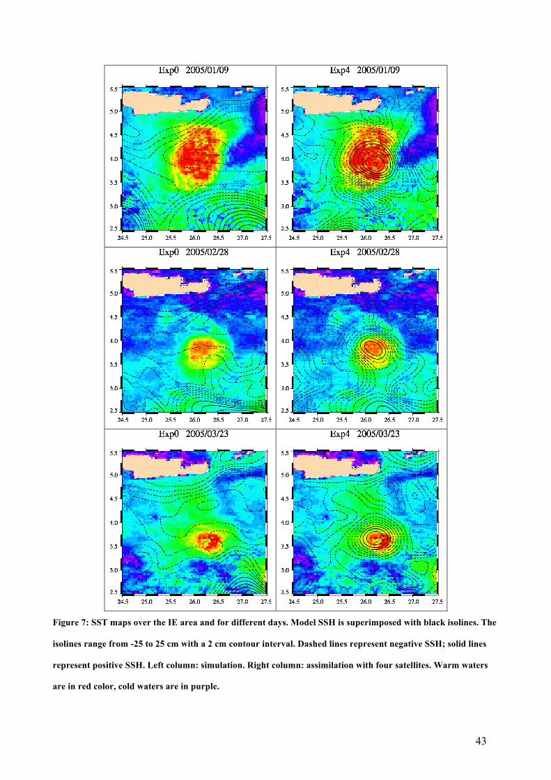
We show now the impact of altimetric data assimilation in the representation of specific structures
of the circulation. This is the case, for example, of the Ierapetra Eddy (IE), usually located off the
southeastern corner of Crete (Horton et al, 1994). This important structure of the circulation is
known to be very energetic and presents an important annual and interannual variability. It can
detach from its usual position to migrate into the central Levantine basin (Larnicol et al., 2002;
Hamad et al., 2005). Without assimilation (exp0) the IE is misplaced and weak, if not absent in the
model simulation (Figure 7). Actually, IE formation processes are quite complex since they involve
at least wind forcing (Horton et al, 1994) and water flow trough the straits of the Eastern Cretan Arc
(Horton et al, 1997), while other forcings have also been claimed such as bottom topography and
water circulation in the Nord-Western Levantine basin (Alhammoud, 2005). On the contrary, the
assimilation of altimeter data introduced the IE in the analysis estimate. The position of the IE for
different days is given in Figure 7 superimposed to SST data. At the beginning of the studied
period, IE was present in the simulation pressed against the south-eastern corner of Crete (see
snapshot for the 06/10/2004). Then, it detached from this position and slowly migrates southward.
At the beginning of December 2004 it was centered around 26.25°E/34°N and it was visible around
26.25°E/33.5°N at the end of March 2005. This behavior is similar to what has been known from

19
the literature. The model analyses reproduce this behavior while the model simulation is seldom
capable to resolve it.
Another improvement in the representation of eddies is shown for two anticyclonic eddies of the
Algerian current. In Figure 8 we show chlorophyll satellite data overlayed on the sea level analyses:
one eddy is located around 2.45°E/36.9°N and the second at 3.4°W/37.1°N. Without assimilation,
the model simulation has a weak anticyclonic flow field detached from the coasts that does not
correspond to the position and shape of the maxima in chlorophyll. As expected, the analysis
improves with respect to the simulation if J1 (Exp1) and then EN (Exp2a) are assimilated since the
position of the anticyclonic structures seems to match better the chlorophyll observations. Contrary
to what is observed with EN, the use of TP as second satellite (Exp2b) seems to degrade the model
output since the intensity of the western eddy is decreased and the eastern nearly disappears. On the
contrary, combining TP with J1 and EN (Exp3) improves the representation of both eddies. Finally,
the optimum analysis is obtained assimilating the fourth altimeter G2 (Exp4) and a nearly perfect
correspondence of the two eddies is observed between the analysed anticyclones and chlorophyll
observations.
b. Impact of the number of altimeters on temperature and salinity analyses
In order to analyze the impact of multi-mission SLA assimilation on the temperature and salinity
analysis fields, we compared the analyses of Exp0-Exp4 with Argo profiles as discussed in section
2.c.
Results are reported in Table 4 for the different experiments. As said before (§3), assimilation of
SLA only (Exp4) has a negative impact on AMO temperature bias and rms errors with respect to
Exp0. For salinity, the assimilation of SLA with respect to the simulation has always a positive
impact. As shown in Table 4, smaller errors for salinity are obtained when 4 satellites are
assimilated and the error is decreased by the addition of each satellite.

20
The contribution of each satellite to the temperature reconstruction is more difficult to interpret: the
specific combination of satellites seems to have different and contrasting impacts on the
temperature reconstruction errors. A positive impact is observed with TP is used as a second
altimeter for both bias and rms but a larger decrease in rms is obtained with the addition of EN as a
second satellite. However when both EN and TP are added to J1 (Exp3) the impact is small or even
negative with respect to the single satellite case (Exp2a). If G2 is used as a fourth satellite, the rms
of AMO for temperature decreases, showing that even G2 has a positive impact on the quality of
the temperature analyses.
In terms of the impact of the different satellites on the quality of temperature and salinity
reconstruction, our analysis is far from being conclusive. However if XBT and ARGO observations
are combined to whatever combination of satellite SLA observations, the bias and rms errors in
temperature and salinity profiles are always decreased (not shown). In section 2b we also point out
that the absolute value of the bias and the rms errors are now close to the observational error limits
for the satellite SLA and this limits our capability to understand small changes due to the addition
of single satellites.
5. Summary and Conclusions
This study has shown the impact of SLA assimilation on the quality of the analyses produced by an
operational assimilation scheme in the Mediterranean Sea. A background error covariance matrix
with a high spatial resolution was especially developed for this study, giving an improvement in the
analyses reconstruction when all data, SLA and temperature and salinity profiles are assimilated.
Experiments were performed with five different altimeter combinations involving one to four
satellites.

21
The experiments highlight the importance of multi-satellite data assimilation in terms of quality of
the analyses, measured as bias and rms of differences between the analyses and the observations
(AMO). In comparison with the model simulations (Exp0), the assimilation of SLA observations by
one altimeter reduces the mean rms of AMO more than 13%. The impact of the assimilation of a
second satellite is nearly as important as for the first satellite with more than 12% reduction of the
mean rms of AMO. The impact of a second satellite especially underlines the complementarity with
the first satellite, when a major rms reduction is locally observed in points where the first satellite
assimilation introduced a rms increase. Impacts of a third and fourth altimeter are lower, but
reductions of the AMO rms for SLA of 3% by each satellite are indicated. In some energetic areas,
like the Algerian current system, the assimilation of observations from the forth satellite reduced the
rms of AMO by more than 10%.
The results obtained differentiate between spatial and temporal satellite sampling schemes. It is
shown that high spatial resolution combined altimeters have a greater impact on the analyses.
Actually, it is shown that EN as second satellite in addition to J1 improves the analyses more than
TP added to J1. Moreover, the impact of G2 as fourth satellite is also important, or even a little bit
more significant than TP as third satellite. This is probably due to the high spatial resolution of the
model, which allows the resolution of mesoscales which are better corrected by the high across
track resolution of EN. This result could support the concept of multi-mission altimetric monitoring
done by complementary horizontal resolution satellites.
Comparison with independent temperature and salinity profiles confirms that the assimilation of
more satellites improves the quality of the analyses especially for salinity. The result is more
questionable for temperature, an issue that will be treated in the future.
The EKE significantly increases by the assimilation of one altimeter. However, contrary to what
was observed from altimeter reconstructed fields without data assimilation (Pascual et al., 2007),
once specific structures are introduced into the model with the assimilation of the first satellite,

22
assimilation of additional altimeter data does not lead to significant increase of the mean EKE. This
might be associated to the specific model resolution which allows a different dynamical adjustment
of the assimilation corrections.
Our study shows that the inclusion of each of four altimeters has a significant impact on the
accuracy of the analyses. We argue that the impact of the number of satellites on the data
assimilation scheme depends the data assimilation scheme approximations and the model capability
to absorb the information from the observations. In the future the oceanographic models will have
even higher horizontal resolutions. Therefore, we may expect that in the future the impact of
additionally altimeters should be re-evaluated and assessed in light of the different model and
analysis schemes.

23
References
Alhammoud B., 2005: Circulation générale océanique et variabilité à méso-échelle en Méditerranée
Orientale: Approche numérique. Thèse de Doctorat de l'Université de la Méditerranée - Aix-
Marseille II.
Artale, V., D. Iudicone, R. Santoleri, V. Rupolo, S. Marullo, and F. D’Ortenzio, 2002: Role of
surface fluxes in ocean general circulation models using satellite sea surface temperature: validation
of and sensitivity to the forcing frequency of the Mediterranean thermohaline circulation. J.
Geophys. Res., 107, 3120–3144.
Benkiran, M., 2007: Altimeter data assimilation in the Mercator Ocean System. Mercator Ocean
Quarterly Newsletter, 25, 32-39.
Berry, P.J., and J.C. Marshall, 1989: Ocean modelling studies in support of altimetry. Dynamics of
Atmospheres and Oceans, 13, 269-300.
Buongiorno Nardelli, B., Larnicol, G., D’Acunzo, E., Santoleri, R., Marullo, S., and Le Traon, P.
Y., 2003: Near Real Time SLA and SST products during 2-years of MFS pilot project: processing,
analysis of the variability and of the coupled patterns, Ann. Geophys., 21, 103–121.

24
Carrère, L., and F. Lyard, 2003: Modeling the barotropic response of the global ocean to
atmospheric wind and pressure forcing – comparisons with observations. Geophys. Res. Lett., 30,
1275, doi:10.1029/2002GL016473.
Chelton, D., and M. Schlax, 2003: The Accuracies of Smoothed Sea Surface Height Field
Constructed from Tandem Satellite Altimeter datasets. J. Atmo. and Ocean. Techn., 20, 1276-1302.
Cooper, M, Haines, K., 1996: Data assimilation with water property conservation. J. Geophys. Res.
101, 1059-107.
De Mey, P., and A. Robinson, 1987: Assimilation of altimeter eddy fields in a limited-area
quasigeostrofic model, J. Phys. Oceanogr., 17, 2280–2293.
Demirov, E., Pinardi, N., Fratianni, C., Tonani, M., Giacomelli, L.,and De Mey, P.: Assimilation
scheme of the Mediterranean Forecasting System: operational implementation, 2003: Ann.
Geophys., 21,189–194.
Dobricic S., N. Pinardi, M. Adani, A. Bonazzi, C. Fratianni, and M. Tonani, 2006: Mediterranean
Forecasting System: an improved assimilation scheme for Sea Level Anomaly and its validation. Q.
J. Roy. Met. Soc. 131, 3627 - 3642, doi:10.1256/qj.05.100.
Dobricic, S., 2005: New mean dynamic topography of the Mediterranean calculated from
assimilation system diagnostics. Geophys. Res. Lett., 32, L11606, doi:10.1029/2005GL022518.

25
Dobricic S., N. Pinardi, M. Adani, M. Tonani, C. Fratianni, A. Bonazzi, and V. Fernandez, 2007:
Daily oceanographic analyses by Mediterranean Forecasting System at the basin scale, Ocean Sci.,
3, 149–157.
Dobricic, S., and N. Pinardi, 2008: An oceanographic three-dimensional variational data
assimilation scheme. Ocean Modelling, 22, 89-105.
Ducet N., P.-Y. Le Traon, G. Reverdin, 2000: Global high-resolution mapping of ocean circulation
from TOPEX/Poseidon and ERS-1 and -2, J. Geophys. Res.,105, 19,477–19,498, 2000.
Ezer T. And G. L. Mellor, 1994: Continuous assimilation of Geosat altimeter data into a three-
dimensional primitive equation Gulf Stream model, J. Phys. Oceanogr., 24, 832-847.
Fukumori, I., R. Raughunath, L. Fu, and Y. Chao, 1999: Assimilation of TOPEX/Poseidon
altimeter data into a global ocean circulation model: How good are the results?, J. Geophys. Res.,
104, 25 647–25 665.
Fukumori, I., D. Menemenlis, and T. Lee, 2006: A near-uniform basin-wide sea level fluctuation of
the Mediterranean Sea. J. Phys. Oceanogr., 37, 338-358.
Haines, K., 2002. Assimilation of satellite altimetry in ocean models. In: ‘Ocean Forecasting:
conceptual basis and applications’, N.Pinardi and J.D.Woods (Eds.), Springer, 472 pp.

26
Hamad, N., C. Millot and I. Taupier-Letage, 2005: The surface circulation in the eastern basin of
the Mediterranean Sea. Sci. Mar., 70, 457-503.
Holland W. R. And P. Malanotte-Rizzoli, 1989: Assimilation of altimeter data into an ocean
circulation model: Space versus time resolution studies, J. Phys. Oceanogr., 19, 1507-1534.
Horton, C., J. Kerling, G. Athey, J. Schmitz, and M. Clifford, 1994: Airborne expendable
bathythermograph surveys of the eastern Mediterranean. J. Geophys. Res., 99, 9891–9905.
Horton, C., Clifford, M., and Schmitz, J.,1997: A real-time oceanographic nowcast/forcast system
for the Mediterranean Sea. J. Geophys. Res, 102(C11), 25123-25156.
Ivchenko, V. O., S. D. Danilov, D. V. Sidorenko, J. Schröter, M. Wenzel, and D. L. Aleynik, 2007:
Comparing the steric height in the Northern Atlantic with satellite altimetry. Ocean Science, 3, 485-
490.
Larnicol, G., N. Ayoub, P.-Y. Le Traon, 2002: Major changes in the Mediterranean sea level
variability from seven years of Topex/Poseidon and ERS-1/2 data. J. Mar. Sys., 33-34, 63-89.
Lermusiaux P.F.J., P. Malanotte-Rizzoli, D. Stammer, J. Carton, J. Cummings, A.M. Moore, 2006 :
Progress and Prospects of U.S. Data Assimilation in Ocean Research ?. Oceanography, Special
issue on Advances in Computational Oceanography, T. Paluszkiewicz and S. Herper Eds., Vol. 19,
1, 172-183.

27
Le Traon, P.-Y., and F. Ogor, 1998: ERS-1/2 orbit improvement using TOPEX/POSEIDON: the 2
cm challenge. J. Geophys. Res., 103, 8045-8057.
Le Traon, P.-Y., 2002. Satellite oceanography for ocean forecasting. In: ‘Ocean Forecasting:
conceptual basis and applications’, N.Pinardi and J.D.Woods (Eds.), Springer, 472 pp.
Le Traon, P.-Y., and P. Gauzelin, 1997: Response of the Mediterranean Mean Sea Level to
Atmospheric Pressure Forcing. J. Geophys. Res., 102, 973-984.
Madec G., P. Delecluse, M. Imbard, and C. Levy, 1998: OPA 8.1 general circulation model
reference manual. Technical report 11, Notes de l'IPSL, Université P. et M. Curie, B102 T15-E5, 4
place Jussieu, Paris cedex 5, France.
Masina, S., N.Pinardi and A.Navarra, 2001. "A global ocean temperature and altimeter data assimilation system for studies of climate variability", Climate Dynamics, 17, pp. 687-700.
Mellor, G. L. and T. Ezer, 1991: A Gulf Stream model and an altimetry assimilation scheme, J.
Geophys. Res., 96, 8779-8795.
Mellor, G. L. and T. Ezer, 1995: Sea level variations induced by heating and cooling: An evaluation
of the Boussinesq approximation in ocean models, J. Geophys. Res., 100(C10), 20,565-20,577.
Ménard, Y., L.-L. Fu, P. Escudier, F. Parisot, J. Perbos, P.Vincent, S. Desai, B. Haines and G.
Kunstmann, 2003: The Jason-1 Mission. Marine Geodesy, 26, 131-146.

28
Millot, C., 1999: Circulation in the Western Mediterranean Sea. J. Mar. Syst., 20, 423-442.
Millot, C., and I. Taupier-Letage, 2005: Circulation in the Mediterranean Sea. The Handbook of
Environmental Chemistry, Volume 5K, 29-66.
Oddo, P., M.Adani, N.Pinardi, C. Fratianni, M. Tonani, D. Pettenuzzo, 2009. A Nested Atlantic-
Mediterranean Sea General Circulation Model for Operational Forecasting. Ocean Sci., 5, 461-473.
Pascual, A., M.-I. Pujol, G. Larnicol, P.-Y. Le Traon, M.-H. Rio, 2007: Mesoscale mapping
capabilities of multisatellite altimeter missions: First results with real data in the Mediterranean Sea.
J. Mar. Sys., 65, 190-211.
Pinardi N., I. Allen , E. Demirov , P. De Mey , G. Korres , A. Lascaratos , P.-Y. Le Traon , C.
Maillard , G. Manzella , and C. Tziavos, 2003: The Mediterranean ocean forecasting system: first
phase of implementation (1998–2001), Ann. Geophys., 21, 3–20.
Pinardi, N., C. Fratianni and M. Adani, 2008. “Usage of real time observations in an operational
ocean data assimilation system: the Mediterranean case”, In: “Real-Time coastal observing systems
for ecosystem dynamics and harmful algal blooms: theory, instrumentation and modelling”,
M.Babin, C.S. Roesler and J.J.Cullen, Unesco Publ., pp 733-763.

29
Pinardi, N., et al., 2009. The Mediterranean Operational Oceanography Network, Bulletin of the
American Meteorological Society, submitted.
Poulain, P.-M., Barbanti, R., Font, J., Cruzado, A., Millot, C., Gertman, I., Griffa, A., Molcard, A.,
Rupolo, V., Le Bras, S., and Petit de la Villeon, L., 2007: MedArgo: a drifting profiler program in
the Mediterranean Sea, Ocean Sci., 3, 379-395.
Pujol, M. I.;Larnicol, G., 2005, Mediterranean sea eddy kinetic energy variability from 11 years of
altimetric data, J. Mar. Systems, 58, 121-142.
Rio, M.-H., P.-M. Poulain, A. Pascual, E. Mauri, G. Larnicol, and R. Santoleri, 2007: A Mean
Dynamic Topography of the Mediterranean Sea computed from altimetric data, in-situ
measurements and a general circulation model. J. Mar. Sys., 65, 484-508.
Robinson, A.R. and P.F.J. Lermusiaux, 2001: Data assimilation in Models, Encyclopedia of Ocean
Sciences, Academic Press Ltd., London, 623-634.
Robinson, A.R., W.G. Leslie, A. Theocharis and A. Lascaratos, 2001: Mediterranean Sea
Circulation. Encyclopedia of Ocean Sciences, Academic Press, 1689-1706.
Tonani, M., N. Pinardi, S. Dobricic, I. Pujol, and C. Fratianni,. 2008: A high-resolution free-surface
model of the Mediterranean Sea. Ocean Sci., 4, 1-14.

30

31
Appendix: OceanVar data assimilation scheme
The OceanVar data assimilation scheme (Dobricic and Pinardi 2008) minimizes the following cost
function:
, (A1)
where is the vector of analysis increments, is the matrix of background error covariances,
is the vector of misfits, is the matrix of observational error covariances, is the
tangent linear approximation of the non-linear observational operator , is the vector of
observations and the vector of the background state. Assuming that background and
observational errors are independent and that their corresponding error covariances are Gaussian, at
the minimum of cost function (A1) the analysis state is the most probable for the
given background state , observations , and the corresponding error covariances and . In
order to avoid the inversion of the matrix , a control variable is defined by
, (A2)
where . In the control space the cost function becomes:
. (A3)
Furthermore, matrix is modelled by the sequential application of linear operators:
. Operator consists of vertical EOFs with temperature and salinity error
covariances. Therefore, control space are weights that multiply the vertical EOFs, and
transforms them into vertical profiles of temperature and salinity increments. Vertical EOFs are
eigenvectors with the largest eigenvalues estimated from the variability of a long term model
simulation around its mean value. The vertical profiles of temperature and salinity are further
multiplied by the operator . It models horizontal Gaussian covariances depending on the

32
horizontal distance in the presence of the coastlines. Operator estimates the sea level and
barotropic velocity increments for the given three dimensional structure of temperature and salinity
increments. It consists of a two-dimensional barotropic model forced by the vertically integrated
buoyancy force due to temperature and salinity increments. The model accurately finds the sea level
increments even in areas with the highly variable and shallow bottom topography. Baroclinc
components of velocity are estimated from the geostrophic relationship in the operator . At
coastlines the geostrophic relationship is often incorrect and may produce the non-divergent
velocity increments. The divergence along the coastlines is attenuated by operator which
applies the divergence damping filter. By sequentially applying different linear operators the
weights that multiply vertical covariances of temperature and salinity are transformed into a two
dimensional field of sea level increments and three-dimensional fields of temperature, salinity and
velocity increments by taking into account the coastlines and the bottom topography. The
conversion from the control to the full physical space is performed in each iteration of the
minimization in order to calculate cost function (A3). In addition it is necessary to calculate in each
iteration the gradient of the cost function by applying the adjoint of observational and
transformation linear operators that substitute transpose of matrices in equation:
. (A4)
Once the minimum is found in the control space, the model correction is calculated by applying
equation (A2). OceanVar is a three-dimensional variational scheme, because it applies estimates of
vertical temperature and salinity error covariances that are independent of actual model dynamics.

33
Table 1: Intertrack (in the Mediterranean Sea) and repetitivity characteristics of each altimeter used.
J1 and TP G2 EN
Intertrack in the Med. Sea (km) ∼260 ∼130 ∼65
Repetitivity (day) 10 17 35
Table 2: Summary of the experiments as a function of the number of altimeters.
Experiment Exp0 Exp1 Exp2a Exp2b Exp3 Exp4 Exp4TS Altimeter
used - J1 J1+EN J1+TP J1+EN+TP J1+EN+TP+G2 J1+EN+TP+G2
+ARGO(T/S)+XBT(T)
Table 3: Reduction (in % of the signal) of the absolute bias and rms of AMO for SLA, induced by the use of HR
EOFs with respect to the use of LR EOFs.
Reduction of the absolute bias Reduction of the rms
4 satellites assimilated -61% -45% 4 satellites + ARGO + XBT data assimilated -45% -33%
Table 4: Reduction (in %) of AMO bias and rms in the upper 400m, for temperature and salinity.
LR_EOFs HR_EOFs
Exp0 Exp4
Exp0 Exp4TS
Exp0 Exp4
Exp0 Exp4TS
Exp0 Exp1
Exp1 Exp2a
Exp1 Exp2b
Exp2a Exp3
Exp3 Exp4
Bias T +61% -41% +43% -65.5% +20% +11% -7% -1% -9% Bias S -14% -72% -22% -70% -11% -4% -4% -3% -7% Rms T +8% -27.5% +4.5% -23% +15% -13% -7% +3% 1% Rms S -13% -49% -19% -47% -7% -8% -5% 0 -6%
Table 5: Reduction of the rms of the along track SLA AMO (in %): the difference is calculated along the
different satellite tracks as a function of the different experiments.
Exp0 Exp1
Exp1 Exp2a
Exp1 Exp2b
Exp2a Exp3
Exp3 Exp4
J1 -29.4 -9.3 -3.6 +0.3 -1.6 EN -14.5 -13.8 -11.1 -3.5 -4.8 TP -11.7 -22.7 -24.8 -10.0 -5.2 G2 -14.0 -17.3 -13.1 -4.0 -4.9 All -19.7 -14.6 -11.9 -3.4 -3.5

34
Table 6: Changes in the mean surface EKE over the Mediterranean Sea during January 2005, expressed in % of
the signal.
Exp0 Exp1 Exp1 Exp2a Exp1 Exp2b Exp2a Exp3 Exp3 Exp4 +27% -5% -6% -2% +2%

35
List of Figures
Figure 1: Position of the different ARGO profiles for the period Sept. 2004-March 2005.
Figure 2: Temporal evolution of the 7-day absolute value (top) and rms (bottom) of AMO for SLA.
Continuous thin line: SLA data assimilated with LR EOFs; continuous thick line: SLA data
assimilated with HR EOFs; dashed thin line: SLA, ARGO and XBT data assimilated with LR
EOFs; dashed thick line: SLA, ARGO and XBT data assimilated with HR EOFs.
Figure 3: Vertical distribution of the bias (left) and rms (right) of AMO for temperature profiles.
Figure 4: Vertical distribution of the bias (left) and rms (right) of AMO for salinity profiles
Figure 5: Temporal evolution of the rms of AMO (in cm) using along track satellite data. From the
upper panel downward: differences along J1, EN, TP and G2 tracks for the different experiments of
Table 2.
Figure 6: Spatial distribution of the relative reduction of AMO rms for SLA . Reduction of the rms
is evidenced by negative, green to blue, values.
Figure 7: SST maps over the IE area and for different days. Model SSH is superimposed with black
isolines. The isolines range from -25 to 25 cm with a 2 cm contour interval. Dashed lines represent

36
negative SSH; solid lines represent positive SSH. Left column: simulation. Right column:
assimilation with four satellites. Warm waters are in red color, cold waters are in purple.
Figure 8: Maps of Chlorophyll along the Algerian current observed the 09/03/2005. Model SSH is
superimposed with black isolines from the six different experiments. The isolines range from -25 to
25 cm with a 2 cm contour interval. Dashed lines represent negative SSH; solid lines represent
positive SSH. High concentrations chlorophyll are presented in red, low concentrations are in
purple.

37
Figure 1: Position of the different ARGO profiles for the period Sept. 2004-March 2005.
38
Figure 2: Temporal evolution of the 7-day absolute value (top) and rms (bottom) of AMO for SLA. Continuous
thin line: SLA data assimilated with LR EOFs; continuous thick line: SLA data assimilated with HR EOFs;
dashed thin line: SLA, ARGO and XBT data assimilated with LR EOFs; dashed thick line: SLA, ARGO and
XBT data assimilated with HR EOFs.

39
Figure 3: Vertical distribution of the bias (left) and rms (right) of AMO for temperature profiles.
Figure 4: Vertical distribution of the bias (left) and rms (right) of AMO for salinity profiles.

40
Figure 5: Temporal evolution of the rms of AMO (in cm) using along track satellite data. From the upper panel
downward: differences along J1, EN, TP and G2 tracks for the different experiments of Table 2.

41
Figure 6: Spatial distribution of the relative reduction of AMO rms for SLA . Reduction of the rms is evidenced
by negative, green to blue, values.

42
43
Figure 7: SST maps over the IE area and for different days. Model SSH is superimposed with black isolines. The
isolines range from -25 to 25 cm with a 2 cm contour interval. Dashed lines represent negative SSH; solid lines
represent positive SSH. Left column: simulation. Right column: assimilation with four satellites. Warm waters
are in red color, cold waters are in purple.

44
Figure 8: Maps of Chlorophyll along the Algerian current observed the 09/03/2005. Model SSH is superimposed
with black isolines from the six different experiments. The isolines range from -25 to 25 cm with a 2 cm contour
interval. Dashed lines represent negative SSH; solid lines represent positive SSH. High concentrations
chlorophyll are presented in red, low concentrations are in purple.