Impact of mIcrobIal DIstrIbutIons on fooD safety

ILSI EuropeReport Series

Commissioned by the ilsi Europe Risk Analysis in Food Microbiology Task Force

About ILSI / ILSI Europe

Founded in 1978, the International Life Sciences Institute (ILSI) is a nonprofit, worldwide foundation that seeks to improve the well-being of the general public through the advancement of science. Its goal is to further the understanding of scientific issues relating to nutrition, food safety, toxicology, risk assessment, and the environment. ILSI is recognised around the world for the quality of the research it supports, the global conferences and workshops it sponsors, the educational projects it initiates, and the publications it produces. ILSI is affiliated with the World Health Organization (WHO) as a non-governmental organisation and has special consultative status with the Food and Agricultural Organization (FAO) of the United Nations. By bringing together scientists from academia, government, industry, and the public sector, ILSI fosters a balanced approach to solving health and environmental problems of common global concern. Headquartered in Washington, DC, ILSI accomplishes this work through its worldwide network of branches, the ILSI Health and Environmental Sciences Institute (HESI) and its Research Foundation. Branches currently operate within Argentina, Brazil, Europe, India, Japan, Korea, Mexico, North Africa & Gulf Region, North America, North Andean, South Africa, South Andean, Southeast Asia Region, as well as a Focal Point in China.

ILSI Europe was established in 1986 to identify and evaluate scientific issues related to the above topics through symposia, workshops, expert groups, and resulting publications. The aim is to advance the understanding and resolution of scientific issues in these areas. ILSI Europe is funded primarily by its industry members.

This publication is made possible by support of the ILSI Europe Task Force on Risk Analysis in Food Microbiology, which is under the umbrella of the Board of Directors of ILSI Europe. ILSI policy mandates that the ILSI and ILSI branch Boards of Directors must be composed of at least 50% public sector scientists; the remaining directors represent ILSI’s member companies. Listed hereunder are the ILSI Europe Board of Directors and the ILSI Europe Task Force on Risk Analysis in Food Microbiology industry members.

ILSI Europe Board of Directors

Non-industry members

Prof. D. Bánáti, Central Food Research Institute (HU)Prof. A. Boobis, Imperial College of London (UK)Prof. G. Eisenbrand, University of Kaiserslautern (DE)Prof. A. Grynberg, Université Paris Sud – INRA (FR)Dr. I. Knudsen, Danish Institute for Food and Veterinary Research (retired) (DK)Prof. M. Kovac, Ministry of Agriculture (SK)Prof. em. G. Pascal, National Institute for Agronomic Research – INRA (FR)Prof. V. Tutelyan, National Nutrition Institute (RU)Prof. G. Varela-Moreiras, University San Pablo-CEU of Madrid (ES)Prof. em. P. Walter, University of Basel (CH)

ILSI Europe Risk Analysis in Food Microbiology Task Force industry members

Industry members

Dr. J. Boza Puerta, Coca-Cola Europe (BE)Mr. C. Davis, Kraft Foods (CH)Mr. R. Fletcher, Kellogg Europe (IE)Dr. G. Kozianowski, Südzucker/BENEO Group (DE)Dr. G. Meijer, Unilever (NL)Prof. C. Shortt, McNeil Nutritionals (UK)Dr. J. Stowell, Danisco (UK)Dr. G. Thompson, Danone (FR)Prof. P. van Bladeren, Nestlé (CH)Dr. P. Weber, DSM (CH)

Barilla G. & R. FratelliDanoneH J HeinzKraft Foods MarsMcDonald’s EuropeNestléUnilever

Impact of mIcrobIal DIstrIbutIons on fooD safety

By John Bassett (Coordinating author)

CommISSIonEd by THE ILSI EURoPE RISk AnALySIS In Food mICRobIoLogy TASk FoRCE

mAy 2010

© 2010 ILSI Europe

This publication may be reproduced for non-commercial use as is, and in its entirety, without further permission from ILSI Europe. Partial reproduction and commercial use are prohibited without ILSI Europe’s prior written permission.

“A Global Partnership for a Safer, Healthier World.®”, the International Life Sciences Institute (ILSI) logo image of the microscope over the globe, the word mark “International Life Sciences Institute”, as well as the acronym “ILSI” are registered trademarks of the International Life Sciences Institute and licensed for use by ILSI Europe. The use of trade names and commercial sources in this document is for purposes of identification only and does not imply endorsement by ILSI Europe. In addition, the views expressed herein are those of the individual authors and/or their organisations, and do not necessarily reflect those of ILSI Europe.

For more information about ILSI Europe, please contact

ILSI Europe a.i.s.b.l.Avenue E. Mounier 83, Box 6B-1200 BrusselsBelgiumPhone: (+32) 2 771 00 14Fax: (+32) 2 762 00 44E-mail: info@ilsieurope.beWebsite: http://www.ilsi.org/Europe

Printed in Belgium

D/2010/10.996/18

ISBN 9789078637202

Contents

1. AbstrAct 4

2. IntroductIon 5

3. MechAnIsMs InfluencIng spAtIAl dIstrIbutIons of MIcroorgAnIsMs 7

3.1 contamination 7 3.2 Microbial growth 9 3.3 Microbial death 10 3.4 Joining 11 3.5 Mixing 11 3.6 fractionation 12 3.7 combining two or more mechanisms 12

4. stochAstIc dIstrIbutIons 15

4.1 scale of analysis and types of distributions 15 4.2 Mixtures of distributions 16 4.3 spatial and frequency distributions 16 4.4 criteria for suitability of frequency distributions 19 4.5 comparison of distributions 29

5. IMpAct of MIcrobIAl dIstrIbutIons on publIc heAlth: effect of clusterIng And “tAIls” 34

5.1 the effect of clustering 34 5.2 effect of a frequency distribution of the exposure 37 5.3 comparison of the effects of various distributions and various degrees of clustering 42 5.4 conclusion 44

6. IMpAct of MIcrobIAl dIstrIbutIons on perforMAnce obJectIves And MIcrobIologIcAl crIterIA 45

6.1 performance objectives 45 6.2 Microbiological criteria 46 6.3 Attributes sampling plans 48

7. dIscussIon, conclusIons And recoMMendAtIons 52

8. MAtheMAtIcAl Annex 55

8.1 normal distribution 55 8.2 lognormal distribution 55 8.3 gamma distribution 56 8.4 poisson distribution 56 8.5 negative binomial distribution 56 8.6 poisson-lognormal distribution 57 8.7 converting between distributions 57 8.8 Monte carlo modelling 59 8.9 Impact of microbial distributions and dose-response on public health 60

9. references 62

Authors: John bassett, unilever (uK), tim Jackson, nestlé (us), Keith Jewell, campden brI (uK), Ida Jongenburger, Wageningen university (nl) and Marcel Zwietering, Wageningen university (nl)Scientific Reviewer: richard Whiting (us)Report Series Editor: Kevin Yates (uK)Coordinator: pratima Jasti, IlsI europe (be)

Impa

ct o

f mIc

ro

bIa

l dIst

rIb

ut

Ion

s on fo

od s

afet

y

3

4

1. AbstrACt

ot much is known about how microorganisms are physically distributed in foods, yet these distributions determine both the likelihood that a foodstuff will cause illness and the consequential public health burden. When food is sampled in an

effort to reduce the risk of causing illness, the effectiveness of the sampling programme is related to the spatial distribution of the microorganisms that are being sampled for. In the absence of exact knowledge, generalising assumptions are often made as to the nature of the distributions. Better insight into the actual microbiological distributions may help to improve food safety management decision-making.

This document discusses mechanisms impacting on physical distributions of microorganisms in foods, characteristics and suitability of frequency distributions employed to model microbial distributions, and the impact of both physical and frequency distributions on illness risk and food safety management criteria. It examines the more common frequency distributions used and evaluates their strengths and weaknesses for modelling real situations against specific criteria.

It can be concluded that the Poisson Lognormal and the Poisson-Gamma (Negative Binomial) are the most suitable distributions given the criteria outlined. However, the ultimate choice must largely depend on how well they fit actual observations.

In many cases the choice of the distribution does not have a large impact on the estimated risk and it is the arithmetic mean that mainly determines the overall risk level. It is then the right hand tail of the exposure distribution that largely determines the cases of illness, so the very low prevalence high doses are substantially determining risk. In certain situations, however, the choice of the distribution impacts significantly on the magnitude of the risk. In those cases a clustered contamination can result in comparatively lower numbers of illnesses than is the case for randomly or regularly distributed contaminations. Therefore, it is relevant to have a good understanding of a situation or to have concrete data at hand that can help decide which type of distribution is most appropriate for particular situations.

Clustering, as evidenced by a change in the standard deviation for a constant mean, has a critical effect on the acceptance probability for typical microbiological criteria and, therefore, the choice of frequency distributions used to model microbial distributions has a substantial effect on the evaluation of microbiological criteria. Also the ratio between the within-batch variability and the between-batch variability has a large impact on the effectiveness of sampling.

Data from multiple quantitative measurements of individual batches would help evaluate the degree of clustering that actually happens in a food system and enable a determination of the most appropriate frequency distributions. However, such data are seldom published. In their absence, it would be advantageous to see more evaluations of approaches to utilising the various distributions in risk assessments and to the setting of risk management targets or microbiological criteria in order to overcome some of the limitations inherent in our assumptions.

Imp

ac

t o

f m

Icr

ob

Ial

dIs

tr

Ibu

tIo

ns o

n f

oo

d s

afe

ty

N

5

Impa

ct o

f mIc

ro

bIa

l dIst

rIb

ut

Ion

s on fo

od s

afet

y

2. introduCtion

icroorganisms in food can be harmless or even beneficial for products and the consumer. Nevertheless, both industry and government expend considerable effort to ensure that microorganisms detrimental to food quality or consumer safety are

eliminated or otherwise controlled in food. Industry utilises food safety management systems such as good hygienic practices, good manufacturing practices and Hazard Analysis and Critical Control Point (HACCP) to ensure this. Governments, via Codex Alimentarius (Codex), have been introducing several new risk-based metrics for food safety management (FAO/WHO, 2006; CAC, 2007). These metrics are the so-called Appropriate Level of Protection (ALOP), Performance Objective (PO) and Food Safety Objective (FSO), which supplement existing management tools, such as microbiological criteria, and are meant to drive further reduction of the public health burden of disease. Tools, such as Microbiological Risk Assessment (MRA) and microbiological sampling, underpin the food safety management concepts utilised by both government and industry. While it is understood that no practical amount of sampling and testing for harmful microorganisms in food can assure the safety of such food, important clues regarding food safety and the possible impact of contaminated food on public health can be derived by assessing the likely presence of harmful microorganisms. These clues are key to making adequate decisions in food safety management.

Importantly, how microorganisms are physically distributed in a food (i.e., their spatial distribution) determines the value of the data on prevalence and/or concentration, obtained through sampling and testing, for informing food safety management decision-making (e.g., for lot acceptance or for process control) and, ultimately, their value for determining the associated public health burden. In general, we have little factual insight into the actual spatial distribution of microorganisms in foods and often generalising assumptions are made that have become commonplace in day-to-day food safety management. While this has served governments and food industry well for many years, it should be stressed that better insight into the microbiological distributions in food matrices may help further to improve food safety management decision-making (in line with the introduction of the new risk-based metrics).

Understanding spatial distributions of (harmful) microorganisms is vital for establishing proper microbiological criteria and obtaining a realistic view of the performance of the associated sampling plans. It is likewise key for setting and verifying risk-based metrics such as POs and FSOs, and for accurate prediction of public health outcomes using MRA. In all these activities, mathematical techniques (e.g., advanced calculations and predictive models) are often used. These may include techniques, such as frequency distributions, to represent the physical distribution of microorganisms in the food concerned. As with many other choices, the choice of the type of frequency distribution to be used has an important impact on the outcome of the calculations and how well it reflects reality. An assumption often used is that microorganisms are distributed lognormally or according to the Poisson frequency distribution. While there is some mechanistic support for the use of these distributions, there is little examination of the impact of the choice of frequency distribution on food safety management decisions (e.g., establishing and interpreting microbiological criteria) or the setting of public health policy. As one example, clustering of microorganisms is an important phenomenon occurring in practice that currently is not well considered. One aim of the current report, therefore, is to discuss options for better including this phenomenon in modelling the spatial distribution of microorganisms, such that it is better taken into account in making food safety management decisions and deriving risk-based metrics or related targets (microbiological criteria).

M

6

This document discusses several physical (spatial) distributions of microorganisms found in foods and the possible mechanisms that may have led to these distributions. It then provides an appraisal of a number of distinct frequency distributions that may be used to describe and represent the spatial distributions and proposes certain criteria for determining the most appropriate frequency distribution(s). In effect, the document outlines the frequency distributions commonly used in modelling spatial distribution and examines the advantages and disadvantages associated with each. Examples of the likely impact of the actual physical distribution and the choice of frequency distribution on public health predictions and food safety management decision-making (e.g., microbiological criteria) will be provided, specifically considering the importance of being able to include low concentrations of pathogens and the phenomenon of clustering in modelling. Finally, conclusions and recommendations relevant for both risk assessors and risk managers will be presented.

Imp

ac

t o

f m

Icr

ob

Ial

dIs

tr

Ibu

tIo

ns o

n f

oo

d s

afe

ty

7

Impa

ct o

f mIc

ro

bIa

l dIst

rIb

ut

Ion

s on fo

od s

afet

y

3. MeChAnisMs influenCing spAtiAl distributions of MiCroorgAnisMs

rom the initial microbial flora of raw material to consumption by the consumer, food products are exposed to a series of processes and related mechanisms that influence the level (i.e., concentration and/or prevalence) and spatial distribution of microorganisms.

Described here are six of these mechanisms that can have an impact on the spatial distribution of microorganisms: contamination, microbial growth, microbial death, joining, mixing and fractionation. These mechanisms are similar to those identified by Nauta (2001).

Each mechanism can work separately, but more often mechanisms work in combination, impacting the microbial level and distribution within a foodstuff. These mechanisms are described in sections 3.1 to 3.6, along with their likely impact. In section 3.7 an example of processing a hamburger patty is presented. It combines several of the six mechanisms.

3.1 Contamination

Contamination is the transfer of microorganisms onto a foodstuff from an external source. The contamination of foodstuffs generally occurs on the surface of a product, and often results in an uneven spatial distribution of microorganisms.

The microbial flora on the surfaces of animals or plants is influenced by a variety of factors, such as local climate, geographical region, agricultural practices and health status of the animal or plant. Raw materials manufactured from animal origin, such as milk, meat or eggs, may be contaminated by microorganisms present on the animal’s skin and faeces during collection or primary processing. Raw materials of plant origin may contain microorganisms present in the soil, water and manure, in which they were grown. Carrots, for example, may become contaminated with Clostridium botulinum spores during primary production. The occurrence and distribution of the microogranism are dependent upon the spore level and its distribution in the soil. C. botulinum may be present in levels, which are not uniform throughout the carrots grown in a field, or even isolated to just a few carrots due to their contact with a localised source of contamination in the soil.

The transfer of microorganisms during a contamination event may occur by contact with contaminated surfaces, air or water. They can be transferred from a number of different sources, via several activities or vehicles, examples of which are:

Equipment and utensilsEquipment and utensils will carry microorganisms on their surfaces. Microbial levels on insufficiently cleaned or dried equipment may increase due to the presence of product residues and water. The transfer of microorganisms from such surfaces occurs as they make direct contact with a food product. As an example, the growth of Enterobacteriaceae may occur on a chocolate production line that has not been adequately cleaned and dried after production. Such contamination could be present at one or several sites on the line.

As the product passes through the area of contamination, the first products may be heavily contaminated and the contamination levels in subsequent products may decline. At the same time, the microbial levels on the equipment surfaces may reduce as the contaminants are transferred to the product.

F

8

Imp

ac

t o

f m

Icr

ob

Ial

dIs

tr

Ibu

tIo

ns o

n f

oo

d s

afe

ty Microbial growth on contaminated surfaces of processing equipment may lead to the development

of biofilms. Cells from bacterial biofilms may detach as single cells or in small portions of biofilm containing cell clusters of over 103 cells. Although larger cell clusters detach less frequently, they contain a disproportionately large proportion of the total detached biomass (Stoodley et al., 2001).

Humans Humans may be a source of contamination through direct contact, such as handling, or indirect contact, such as the generation of aerosols from clothing, movements or sneezing. Such events may occur during collection, manufacturing, distribution or preparation. The level and distribution of the contaminating microorganisms will be influenced by the source and level of contact. For example, a worker whose hands are contaminated with Listeria, may contaminate individually quick-frozen meat that is being placed into assembled meals. The resulting contamination would be of low level and only present in products that contain hand-packed meat.

Water used for rinsing, cleaning and coolingWater can be a source of contamination, through intentional addition, such as ingredient water or irrigation water, or through unintentional addition, such as leaks from cooling water in closed-circuit systems, condensation and subsequent transfer of water droplets onto products or product contact surfaces, or transfer from poor cleaning practices such as high-pressure hoses.

Secondary process water (water used in processing, but not intended for inclusion in products) could become a source of contamination directly into the product stream from leaks in closed-circuit systems. The resulting distribution is dependent upon the size of the leak, the flow of the product stream and the pressure differential between the product and process water source. Contamination from a continuous leak of contaminated secondary process water or wastewater into a tank or product stream would lead to contamination of a large number of sample units and such contamination could be distributed throughout a lot.

Contaminated water used in cleaning equipment could lead to a widely distributed contamination on product surfaces, contaminating a large number of product units that pass over or through the contaminated surface.

Heavily contaminated cooling water could lead to contamination of shelf-stable canned foods through micro-leaks in the cans’ seams. The extent of contamination and resulting spoilage are dependent upon microbial levels in the water and the distribution of cans containing micro-leaks.

Aerosols such as dust, or aerosolised droplets Microorganisms attached to particles, such as dust or aerosolised droplets, may land on food contact surfaces or directly into the food product. In such cases the number of microorganisms on each particle is generally low, while the distribution of contaminants is affected by various factors such as air movement, relative humidity, degree of product exposure, concentration of particulates in the air and nature of the source of contamination of the airborne particles. Aerosols generated by compressed air used in processing or cleaning activities, such as the use of high-pressure hoses, can transfer microorganisms from contaminated surfaces onto products or product contact surfaces.

Packaging materialsAlthough in most cases microbial levels on well-stored and protected packaging materials are relatively low, contamination of packaging materials could be a source of spoilage microorganisms in perishable foods. For example, storage conditions for primary packaging for yoghurt are critical, as mould spores present in dust that settles on poorly stored packaging may lead to product contamination and spoilage.

9

Impa

ct o

f mIc

ro

bIa

l dIst

rIb

ut

Ion

s on fo

od s

afet

y

AnimalsAnimals, such as rodents, birds, insects and other domestic and wild animals, may be a source of contamination, particularly during cultivation and collection of plants and rearing of animals. For example, vegetables may become contaminated with Salmonella due to direct contact with the faeces of birds or other animals in the field. Such contamination is localised to the point of contamination, such as the deposit of bird faeces. Contamination may be spread to other portions of wheat during harvesting.

Animals may also become a source of contamination during processing as rodent, bird and insect pests indirectly contaminate materials or processing environments through droppings, hair and other particulates.

3.2 Microbial growth

Once a food product has been contaminated, microbial growth can transform an initially homogeneous distribution into a more clustered distribution on or within a foodstuff. In contrast with contamination, which occurs on external surfaces, growth can cause the distribution of microorganisms inside the product.

During growth through reproduction, microbial cells may remain attached to each other and form cell clumps or micro-colonies as represented graphically in Figure 3.1 This may, for instance, be due to particular growth characteristics of the microorganisms or to physical constraints of the food matrix. Cells that have the ability to move actively with flagella may overcome such a clustering if the matrix allows their movement. Figure 3.1 Development of cell clumps inside a food product turning a homogeneous distribution into a clustered distribution

Microbial growth can also result in an uneven distribution of microorganisms if growth conditions differ in various parts of the product. This may occur, for example, during the cooling of the foodstuff, where the product temperature in the inside of the food remains high enough to allow growth even as conditions on the outside restrict growth. Alternatively, during thawing, the external temperature may allow growth, while growth inside the product is restricted by colder temperatures (Figure 3.2).

Figure 3.2 Growth of microorganisms near the surface of a food product during thawing

3.3 Microbial death

Microbial death can result from the application of lethal processes (such as thermal processing or the addition of lethal levels of preservatives) or from the adverse effects of changing environmental conditions. Intrinsic product characteristics (e.g., water activity, pH and nutrient availability), and extrinsic product characteristics (e.g., storage temperature or storage atmosphere) could lead to inhibition of microbial growth or (at lethal levels) even complete inactivation (death) of microbial cells.

The effectiveness of lethal processes delivered to a food product may be influenced by a number of factors, including the variations within processing equipment and the dimensions, consistency and thermal diffusivity of the product. For example, during heat treatment some contaminants may survive if the heat has not been sufficiently conducted into the interior of the food product, referred to as a cold spot. Cold spots may be present in different parts or spatial locations of a food, not necessarily in the centre of the food, depending on the type of heating applied (e.g., volumetric heating, microwave heating, radio-frequency heating, etc.). The lethality of preservatives added to a food will vary if the preservative is unevenly distributed in a product, affecting the final distribution of microbial cells. Additionally, differences in the resistance of individual microbial cells could lead to variability of lethality and therefore affect the microbial distribution. Such uneven inactivation would increase the degree of microbial clustering (Figure 3.3). Figure 3.3 Clustered distribution of microorganisms which survived a heat treatment in the centre of a food product

10

Imp

ac

t o

f m

Icr

ob

Ial

dIs

tr

Ibu

tIo

ns o

n f

oo

d s

afe

ty

11

3.4 Joining

Joining two or more materials (e.g., ingredients or food products), each with different microbial distributions, will result in a joined product with a distribution, which is different from the initial microbial populations of the merged materials (Figure 3.4). The overall population of the joined product will be roughly a sum of the populations of the joined materials and the distribution of the overall population will be a function of the way in which joining occurs. For example, several layers joined in tiramisu will result in an overall population distributed according to the way in which the tiramisu components, and thus the original microbial populations, were assembled.

During the production process, joining may be followed by mixing and other processing. For example, during the production of minced meat several pieces of meat are combined, mixed and minced. Figure 3.4 Joining product results in rearrangement of the microorganisms in a food product

3.5 Mixing

When materials or product units are mixed, the original microbial population is relocated throughout the product mass. This is likely to lead to a more random spatial distribution and a changing of the number of cells per portion, for example, per unit of weight or volume (Figure 3.5). In general, mixing will disperse the microbial populations. Mixing can be an active process or it can be a result of, for instance, spontaneous movements caused by temperature or concentration differences in liquids.

Figure 3.5 Mixing the product results in rearrangement of the microorganisms in a food product

The distribution of microorganisms, through the course of producing a batch of minced meat, was investigated by Kilsby and Pugh (1981). In sequential steps, frozen, boned carcass beef was thawed, minced and bowl-chopped. At each step of the process, the levels of microorganisms in 20 random sub-samples were analysed to estimate the number of microorganisms present in the batch. Mixing altered the distribution of microorganisms within the batch of meat; the mean concentration became higher and the variance lower during the minced meat production.

Impa

ct o

f mIc

ro

bIa

l dIst

rIb

ut

Ion

s on fo

od s

afet

y

Besides mechanical mixing, further development of the microbial distribution depends on the consistency of the contaminated product. For liquid, semi-liquid or powder, an initial localised contamination may become more random as a result of turbulence or movements caused by transport. For contamination on solid surfaces, in solid or semi-solid foods, such movements may have no or only a minor effect on distributions. Strong movements, however, may cause this contamination to become dislodged from the surface and transferred to another area of the surface or to another part of the food.

3.6 Fractionation

Fractionation, like mixing, reallocates microorganisms over the resulting product units. For example, during slicing, a chicken filet with localised surface contamination could be divided into fractions of highly contaminated chicken meat and fractions with little or no contamination (Figure 3.6). As another example, when a batch of milk powder, which contains a localised or sporadic contamination, is filled into bags, some of the bags could contain clusters of a contaminating microorganism while others could be free of the microorganism. Fractionation can also encompass procedures that may result in the removal of contaminating microorganisms, for instance when a portion of a food product is discarded or removed by peeling or rinsing.

Nauta proposed mathematical models to describe the effect of mixing and fractionation on the statistical distributions (Nauta, 2005). Figure 3.6 An illustration of a case in which fractionation of a food product results in heavily contaminated fractions and fractions with little or no contamination

3.7 Combining two or more mechanisms

While the six mechanisms described above may work alone, it is more often a combination of these mechanisms that affects the final microbial distribution of a product. At a particular step, the starting microbial distribution will be the microbial distribution resulting from the relevant mechanism(s) at the previous step. In the subsequent steps, mechanisms or sets of mechanisms may have an impact on the final distribution. The distribution of the pathogen Escherichia coli O157:H7 during the production of hamburger patties is an example in which all six mechanisms may contribute to the distribution of the pathogen in the final product. Figure 3.7 illustrates which mechanisms may be involved in sequential process steps, altering the microbial distribution in the specific step and, ultimately, in the hamburger patties.

E. coli O157:H7 may colonise cattle and be present in the faeces of cattle to be slaughtered. Some or all of the cattle in a given herd may be colonised, the colonisation influenced by environmental conditions and herd management practices. Animals from different herds may be intermingled prior to slaughtering, dispersing infected animals among those to be processed and in some cases contaminating additional animals through the contamination of food, water or the environment with faeces of infected animals.

12

Imp

ac

t o

f m

Icr

ob

Ial

dIs

tr

Ibu

tIo

ns o

n f

oo

d s

afe

ty

13

At the abattoir, the cattle are slaughtered and the carcasses divided into cuts. Cross contamination of the carcass surfaces can occur to varying degrees due to actions ocurring during the primary process such as stunning, bleeding, de-hiding, evisceration, washing, cutting, etc.

During further processing, carcasses may be divided into smaller cuts, fractionating the microbial population as a function of the original distribution and the dimensions of the cuts. Contamination may also occur from cutting equipment, workers and water used in cleaning.

During the mixing of meat and spices, cuts, trimmings, spices and other ingredients are combined, merging microbial populations from multiple sources. Subsequently, bowl chopping and/or grinding to prepare comminuted meats will further distribute the contamination from one or more sources of trimmings that are ground together. Fractionation will again occur during the preparation of patties as portions of the combined mass are removed.

During the packaging of the patties, contamination may occur from contaminated packaging equipment, workers and other patties. An initial decline may occur during the freezing process, influenced by the conditions of freezing. The remaining populations may gradually decline during frozen storage, although survival of a sub-population is likely.

When the consumer thaws the hamburger, thawing may allow growth if the thawing temperatures are sufficiently high. In such cases growth will first occur on the surfaces of patties where the temperature is warmer.

In the last step, cooking will result in the death of E. coli O157:H7. The distribution of lethality may be influenced by the variations in density and thickness of the patty. Depending upon the cooking conditions, survival may occur in cold spots in the product that do not receive sufficient heating. Variations in temperatures on a grill or within an oven could also result in undercooking of some units and result in survival.

Impa

ct o

f mIc

ro

bIa

l dIst

rIb

ut

Ion

s on fo

od s

afet

y

Figure 3.7 Overview of likely mechanisms and sources of contamination impacting the distribution of microorganisms for each step in the production process of hamburger patties

Each of the mechanisms described in this chapter may have an impact on the spatial distribution of microorganisms in a food. The following chapter will show the relationship between the spatial distribution and the frequency distribution. Different microbial distributions will be described in terms of their dispersion (spatial distribution) patterns and the stochastic frequency distributions that may be used for modelling those patterns.

14

Imp

ac

t o

f m

Icr

ob

Ial

dIs

tr

Ibu

tIo

ns o

n f

oo

d s

afe

ty

15

4. stoChAstiC1 distributions

hile the previous chapter has indicated how different distributions of microorganisms are likely to arise, this chapter lays out a mathematical framework for describing and representing (‘modelling’) such distributions. It includes a more

formal account and quantitative interpretations of relevant terminology, such as ‘regular’, ‘clustered’ and ‘random’.

4.1 Scale of analysis and types of distributions

It is unlikely that every food portion of a larger bulk contains the same number of microorganisms. Chapters 5 and 6, below, show that variation between portions can affect both food safety and the performance of acceptance sampling plans, even when the overall average is constant, so that the simple average number of microorganisms per portion is not an adequate representation of microbial status. This section considers distributions that might be used to model portion-to-portion variation as well as overall average, providing a more complete representation of the microbial status of a batch. It is necessary first to consider the sizes of the portions and batches of interest, which differ between considerations of food safety and considerations of acceptance sampling plans (microbiological criteria).On a very small scale, comparable to the size of a microogranism (perhaps 10-12 cm3) there are only two kinds of portion, containing an organism or not, so that all possible distributions are clustered. Conversely, large portions can be expected to ‘average out’ small scale clustering, but to reveal larger scale clustering, for example by production runs or production within a particular country. In principle, the presence of clustering can be defined, independently of scale, in terms of the probability of points (organisms) depending on the presence of nearby points (section 4.3 below). In practice, the exact location of organisms is unknown and of little interest. The distribution is deduced from, and its effect mediated by, numbers (or presence) in finite-sized samples.

From the perspective of public health, the portion of interest is that which is actually consumed (e.g., 50 g to 500 g), as this, inter alia, determines the exposure of individual consumers. The batch of interest is that which might be the subject of a risk assessment or be responsible for an outbreak, or which is the subject of food safety management criteria. In an industrial setting this is not likely to be much less than a tonne, but might be as much as hundreds of tonnes.

In the case of acceptance/rejection, the portion of interest is the amount analysed, often smaller than the sample taken (e.g., 0.1 g to 100 g). The batch of interest is that subject to the acceptance/rejection decision, probably of the order of tonnes.

Accordingly, this work considers the variation between portions of size 0.1 g to 500 g within batches of tonnes.

Impa

ct o

f mIc

ro

bIa

l dIst

rIb

ut

Ion

s on fo

od s

afet

y

1. Adjective having a random probability distribution or pattern that can be analysed statistically but not predicted precisely. Origin Greek stokhastikos, from stokhazesthai ‘aim at, guess’ (Soanes, 2003).

W

4.2 Mixtures of distributions

As described earlier, the final distribution of microorganisms in a food is usually the result of multiple distinct mechanisms, having an impact individually or in combination and being active continuously or changing in a discontinuous manner. Even if the individual mechanisms would have produced quite simple frequency distributions, their combination usually results in a more complicated frequency distribution, often a mixture of the simpler distributions. Sometimes, one mechanism might dominate, so that the mixture can be approximated by a simpler distribution.

To model a mixture of simple distributions, or to approximate a mixture by a single simple distribution, it is necessary first to understand those simple distributions. Accordingly, this chapter (4, ‘Stochastic distributions’) concentrates on a number of quite simple ‘standard’ distributions.

Please note, however, that subsection 4.4.2.2, ‘Generalised Poisson distributions’, discusses how simple distributions (and specifically the Poisson frequency distribution) can be generalised to model mixtures of simple distributions. Also, some of the ‘standard’ frequency distributions considered (i.e., the zero-inflated Poisson, Negative Binomial and Poisson-Lognormal distribution) are in fact generalised Poisson distributions and may be suitable for modelling microogranism frequency distributions resulting from combinations of mechanisms.

4.3 Spatial and frequency distributions

Physical or spatial distributions are different from, although related to, frequency distributions. The differences and relationships are illustrated in Figures 4.1, 4.2 and 4.3. In each figure chart (a) represents points quite regularly spread, chart (b) represents points forming a single quite tight cluster against a very low density, random background and chart (c) represents points randomly spread. For ease of representation, these examples are given in two dimensions, but notably the concepts extend directly to three dimensions or even to four when distribution in time is considered as well.

The figures 4.1 and 4.2 show different arrangements of 100 points among 25 ‘portions’. In a food industry context, each portion could be considered a ‘unit’ and the set of 25 portions a ‘lot’, so the figures represent ‘within-a-unit’ and ‘within-a-lot’ variation. Alternatively, each portion could be considered a lot so the figures represent ‘within lot’ and ‘between lot’ variation. Real situations do not have such a simple 2-level dichotomy, but these figures and the subsequent discussion lead to generally applicable conclusions.

Figure 4.1 shows three different spatial distributions of 100 points over 25 portions. Figure 4.2 shows the resulting number of points in each portion; Figure 4.3 shows the resulting frequency distributions (i.e., representing how often each ‘points per portion’ value occurred).

Figure 4.1 Three different spatial distributions of 100 points over 25 portions. a) almost regular b) one cluster c) random

16

Imp

ac

t o

f m

Icr

ob

Ial

dIs

tr

Ibu

tIo

ns o

n f

oo

d s

afe

ty

17

Figure 4.2 Numbers of points in individual portions for the three spatial distributions depicted in Figure 4.1.a) almost regular b) one cluster c) random

Figure 4.3 Frequency distributions for the three spatial distributions depicted in Figures 4.1 and 4.2. Note that chart c) includes a Poisson distribution, which is the frequency distribution corresponding to a uniform random spatial distribution.a) almost regular b) one cluster c) random

Figure 4.1 (spatial distributions of points) contains no values, just the locations of the points. It contains most information, in the sense that Figures 4.2 and 4.3 can be deduced from Figure 4.1, but not vice versa. Figure 4.2 (spatial distributions of values) contains values (the concentrations in each portion) and locations (of portions, not of individual points). Figure 4.3 (frequency distributions) contains information on values, but no information on location. This means that different spatial distributions can produce the same frequency distribution. For example, in the rearrangement of Figure 4.2c shown in Figure 4.2d, the high concentration portions are clustered together, but the frequency distribution is unchanged, Figure 4.3c.

To describe spatial distributions in quantitative terms can be quite difficult; the statistics of ‘spatial processes’ is sophisticated. Several approaches could be used. For instance, the positions of the points could be described by their X-Y coordinates, or by the distances between neighbouring points. One way of characterising spatial distributions is by stating how the chance of finding a point depends upon the closeness of other points. Discussing this approach further leads to a more formal description of the terms ‘regular’, ‘clustered’ and ‘random’.

Impa

ct o

f mIc

ro

bIa

l dIst

rIb

ut

Ion

s on fo

od s

afet

y

d) rearrangement of (c)

18

Imp

ac

t o

f m

Icr

ob

Ial

dIs

tr

Ibu

tIo

ns o

n f

oo

d s

afe

ty a) In regular distributions (e.g., Figure 4.1a), points are less likely close to other points, so that points

are relatively far apart from each other. Although such patterns are relatively unusual in food microbiology, they can occur where contamination occurs following more or less regular patterns, for instance from one contaminated head of a multi-head filler.

b) In clustered distributions (e.g., Figure 4.1b), points are more likely close to other points, so that points are relatively close to each other. Such patterns are quite common in food microbiology, as contamination often occurs in clusters, for instance because of initial contaminants multiplying into micro-colonies, disruption of biofilms, localised growth of microorganisms in non-liquid foods, etc.

c) In uniform random distributions (e.g., Figure 4.1c), points are equally likely close to or far from other points. In this case, therefore, the chance of finding a point is independent of the closeness of other points. Random patterns might result from other patterns by perfect mixing. However, mixing does not result in a regular pattern, although it is tempting to see clusters and other patterns in random arrangements such as Figure 4.1c. This is because the human eye and brain have evolved to see regular patterns. While the points in a random pattern are equally likely everywhere (in other words, the distribution of probability is uniform), they cannot actually be everywhere (so, the distribution of points is not uniform). Uniform random patterns are quite common in food microbiology, for instance in the case of well-mixed liquids or powders. This type of pattern has often been used to represent other spatial patterns, because it is the only information available.

Considering “real” information available;

• Data describing actual spatial positions of individual microorganisms (e.g., as in Figure 4.1) contains most information, and can be converted to per-portion-position or frequency distribution form if required. Unfortunately, such information is very rarely available.

• Data describing spatial positions of portions and their concentrations (e.g., as in Figure 4.2) contains some direct spatial information, and can be converted to frequency distribution form if required. Such information is not common. Where it is available, the concentration data is often presence/absence rather than counts, which limits its value.

• The most commonly available data has no spatial content at all, being simply frequency distributions (e.g., as in Figure 4.3) specifying how often particular concentrations were observed. Again, the concentration data is often presence/absence rather than counts, so that histograms such as Figure 4.3 would have only two bars, 0 and >0.

The word ‘dispersed’ can have different and opposite meanings when describing spatial distributions and frequency distributions. Comparison of Figures 4.1 and 4.3 shows that the most spread out spatial distribution (chart (a), ‘regular’) gives the smallest variation in points per cell, while the most compact spatial distribution (chart (b), ‘clustered’ into a single cluster) gives the greatest variation and the intermediate spatial distribution (chart (c), ‘random’) gives an intermediate variation.

• A more dispersed, less clustered, spatial distribution (e.g., Figure 4.1a) gives a less dispersed, more clustered, frequency distribution (e.g., Figure 4.3a).

• A less dispersed, more clustered, spatial distribution (e.g., Figure 4.1b) gives a more dispersed, less clustered, frequency distribution (e.g., Figure 4.3b).

The variation of values in a frequency distribution (e.g., Figure 4.3) is often called the ‘dispersion’ and measured by the ‘variance’; the average is often represented by the mean. As summarised in Table 4.1 the degree of spatial clustering can often be assessed by comparing the variance and mean of the corresponding frequency distributions; note that ‘under-dispersed’ and ‘over-dispersed’ are widely used with the meanings indicated in Table 4.1.

19

Table 4.1 Relationship between spatial and frequency distributions

Spatial distribution (relative to uniform random)

Frequency distribution (relative to Poisson) Example

more spaced more

concentrated

underdispersed variance <

mean

regular contamination due to

contaminated filler head

uniform random Poisson variance =

mean

perfect mixing

more clustered More right

skewed

overdispersed variance >

mean

local contamination from hand

contact

While earlier in this chapter ‘regular’, ‘clustered’ and ‘random’ spatial distributions were defined in terms of the relative probabilities of finding points closer to and further away from other points, Table 4.1 suggests a set of alternative descriptions in terms of frequency distributions:

a) A regular spatial distribution has a frequency distribution with variance smaller than its mean.

b) A clustered spatial distribution has a frequency distribution with variance greater than its mean.

c) A uniform random spatial distribution has a frequency distribution with variance equal to its mean.

The next subsection considers mathematical models available to represent such different frequency distributions.

4.4 Criteria for suitability of frequency distributions

There are a number of criteria that mathematical distributions used to model frequency distributions of microorganisms should satisfy if they are to represent or approximate spatial distributions well, in real, practical situations.

a) The model outcome should not be negative, as it is not possible to have negative numbers of microorganisms in a food. This criterion can be satisfied when the frequency distribution will give zero probability to negative values.

b) The model should allow zero as an outcome, because it is possible to have no microorganisms in a portion of food. This criterion can be met when the frequency distribution gives a finite probability to zero values.

c) The model outcome should be discrete numbers only, as it is not possible to have parts of microorganisms in a portion as viable units. To satisfy this criterion, the frequency distribution should not assign probability to fractional numbers.

d) The frequency distribution should reduce to, or at least approximate, the Poisson distribution, because it can be shown that the frequency distribution corresponding to the specific case of a uniform, random, spatial distribution (as might be produced by perfect mixing) is a Poisson distribution (described in subsection 4.4.2 below).

e) The frequency distribution should be similar to, or approximate, the Lognormal distribution at high numbers of microorganisms (when there is negligible probability of zero microorganisms). This criterion is suggested because the Lognormal distribution (described in subsection 4.4.3 below) has been widely and successfully used to model microorganisms frequency distributions in many circumstances. Although the frequency distribution of microorganisms must really be discrete (no fractional microorganisms), at high numbers the difference between successive integers is small enough that continuous frequency distributions may be good approximations.

Impa

ct o

f mIc

ro

bIa

l dIst

rIb

ut

Ion

s on fo

od s

afet

y

These five criteria can be used to assess explicitly the suitability of the commonly used frequency distributions, as is done below. However, it should be stressed that any frequency distribution is only an approximation of reality and that, in practice, other criteria will also influence the choice of frequency distribution. Such influences may include familiarity, ease of use, and the level of agreement between the model and actual observations.

Here we consider six types of distribution:

1. Normal distribution

2. Poisson distribution (including generalised Poisson distributions)

3. Lognormal distribution

4. Gamma distribution

5. Negative Binomial distribution (one type of generalised Poisson)

6. Poisson-Lognormal distribution (another type of generalised Poisson)

4.4.1 Normal distributionsThe most commonly used frequency distribution is the Normal distribution (also known as the Gaussian distribution). This type of distribution is depicted in Figure 4.4 and an assessment is provided of whether it complies with the five suitability criteria.

Figure 4.4 A Normal distribution2

a) non-negative; NOb) allows zeros; YESc) discrete; NOd) approximates Poisson; NOe) approximates Lognormal; NO

The Normal distribution does not comply with four out of the five proposed criteria. It, for instance, gives finite probabilities to negative values. The Normal distribution is therefore not suitable either for direct representation of microbial frequencies or to generalise the mean of a Poisson distribution.

4.4.2 Poisson distributionsA single-parameter Poisson frequency distribution is fully defined by its location, e.g., its mean. Its dispersion as measured by variance (which is equal to the square of the standard deviation), is equal to the mean, Figure 4.5 shows a number of Poisson distributions with different means.

20

Imp

ac

t o

f m

Icr

ob

Ial

dIs

tr

Ibu

tIo

ns o

n f

oo

d s

afe

ty

2. In frequency distribution graphs “pdf” means “probability density function” and (for discrete distributions) “pmf” means “probability mass function”. Loosely speaking, these can be thought of as the probability associated with a given value, x.

Impa

ct o

f mIc

ro

bIa

l dIst

rIb

ut

Ion

s on fo

od s

afet

y

21

Figure 4.5 Examples of Poisson distributions

a) non-negative; YESb) allows zeros; YESc) discrete; YESd) approximates Poisson; YESe) approximates Lognormal; NO

A uniform random spatial distribution results in a Poisson frequency distribution. In addition, the Poisson frequency distribution is often used in the absence of anything more appropriate (e.g., based on specific knowledge of the likely spatial distribution), even when a uniform random spatial distribution cannot be assumed.

While the Poisson distribution is the distribution of choice for well-mixed products with low concentrations of microorganisms, the single parameter Poisson distribution does not have the flexibility to model the variations in microbial concentrations seen in practice. For instance, at high concentrations (e.g., above 20 cfu (colony forming units)/portion) a Poisson distribution is essentially symmetrical, while observed distributions of microbial concentrations are often skewed to the right (i.e. indicating that the highest concentrations occur at relatively high frequencies compared to a symmetrical distribution). Generalised Poisson distributions (discussed in subsection 4.4.2.2 below) are more flexible.

4.4.2.1 Under- and over-dispersionThe dispersion (as measured by variance) of a Poisson frequency distribution is equal to its mean. Accordingly, distributions whose variance is less than the mean are often called ‘under-dispersed’ and those whose variance is greater than the mean are called ‘over-dispersed’. In practical terms, over-dispersion of the frequency distribution reflects clustering in the spatial distribution. Under-dispersion then reflects separation in the spatial distribution (here referred to as ‘over-spacing’), meaning that it is more regular than a uniform random distribution. However, under-dispersion is less common than over-dispersion in foods.

Poisson frequency distributions are commonly used in the development of microbiological risk assessments and the establishment/interpretation of microbiological criteria. The degree of over- or

Imp

ac

t o

f m

Icr

ob

Ial

dIs

tr

Ibu

tIo

ns o

n f

oo

d s

afe

ty

22

under-dispersion (clustering or spacing) of a particular distribution as compared to a Poisson distribution can be assessed on the basis of the ratio between the variance and the mean as follows:

− ratio =1 for uniform random spatial distributions,

− ratio >1 for clustered spatial distributions, and

− ratio <1 for over-spaced distributions.

A statistical test (Stoyan and Stoyan, 1994) for the presence of spatial clustering or over-spacing is based on the ‘dispersion index’, I:

For a set of concentrations taken from a Poisson distribution (e.g. where the spatial distribution is uniform random) s2 is expected to be about equal to x, so I is about equal to n. In fact, for such a sample, I is distributed according to a χ2 distribution with n-1 degrees of freedom and if n is greater than 6 and x is greater than 1 then I can be tested against the χ2 distribution. If the cumulative χ2 probability is very small (e.g. less than 0.05) there is statistically significant evidence of over-spacing, and if it is very big (e.g. more than 0.95) there is statistically significant evidence of spatial clustering. Table 4.2 shows the relevant calculations for the frequency distributions in Figure 4.3.

Table 4.2 Calculation and test of dispersion index for distributions in Figure 4.3.

Distribution n s I Cumulative χ2 probability

a)almost regular 25 0.00000 4.000 0.000 <0.00001

b) one cluster 25 9.73824 4.000 536.46 1.00000

c) random 25 1.70783 4.000 18.229 0.20825

N.B.: In the software system Microsoft Excel, the cumulative χ2 probability can be calculated with a formula such as ‘=1 CHIDIST(E2,B2-1)’ where E2 is the cell containing I and B2 is the cell containing n.

4.4.2.2 Generalised Poisson distributionsGeneralised Poisson distributions provide more flexibility than single-parameter Poisson distributions, from which they are derived. Different terms have been used in literature by different authors to describe such combinations of distributions. Alternatives used may include generalised, compound, contagious, aggregate, or mixture distributions. In this report, the term ‘generalised’ is used.

A generalised frequency distribution – specifically a generalised Poisson distribution – can be understood in terms of the ‘parameters’ of the distribution. For a conventional Poisson distribution, the distribution is fully defined by its location and, as a consequence, the Poisson distribution can be defined by a single parameter reflecting ‘location’, usually the mean. In a generalised distribution a parameter of the simple distribution (the only parameter for a Poisson) itself follows a distribution3.

3. Expressed mathematically, a distribution containing a parameter θ, say f(x|θ), can be generalised by weighting it by a distribution for θ, say p(θ), and then integrating with respect to θ to obtain the marginal distribution.

For generalised Poisson distributions, the generalising distribution, p(θ), describes the mean of the Poisson distribution, f(x|λ=θ), so that it is not limited to integer values, although it cannot be negative.

23

Impa

ct o

f mIc

ro

bIa

l dIst

rIb

ut

Ion

s on fo

od s

afet

y

The single-parameter Poisson distribution corresponds to a uniform, random spatial distribution of points, where the mean or expected number of points per portion is constant. One way to allow for clustering to be reflected in a model is to describe the number of clusters by a Poisson distribution and the number of points within each cluster by another distribution; this may also be viewed as a mixture of Poisson distributions with different means, where the means follow another distribution. The total number of points in a given volume then follows a ‘generalised Poisson distribution’. In terms of the five proposed criteria, the generalised Poisson frequency distribution retains the advantages of the single-parameter Poisson, but it is not restricted to having variance equal to its mean and it can model the skewness associated with a Lognormal frequency distribution.

a) non-negative; YESb) allows zeros; YESc) discrete; YESd) approximates Poisson; YESe) approximates Lognormal; IF the generalising distribution is appropriate YES, otherwise NO.

If the generalising frequency distribution is continuous and unimodal (meaning it has only one peak), the resulting generalised Poisson distribution is unimodal. Two types of continuous, generalising distributions are considered below, namely the Gamma distribution (which results in the Negative Binomial; see subsection 4.4.5), and the Lognormal distribution (resulting in the Poisson-Lognormal; subsection 4.4.6). Instead of continuous types, a discrete generalising frequency distribution can also be used, one of which results in the so-called ‘zero-inflated’ Poisson (see subsection 4.4.2.3). Discrete generalising distributions can result in discontinuous and/or multimodal generalised Poisson distributions.

If individual spatial distributions are appropriately modelled by a Poisson frequency distribution, then a generalised Poisson can be an appropriate model for a mixture of distributions.

4.4.2.3 Zero-inflated Poisson distributions.One discretely generalised Poisson distribution is the ‘zero-inflated’ Poisson distribution. This frequency distribution generates more zero values than a single parameter Poisson. An example of a simple form of zero-inflated Poisson distribution is shown in Figure 4.6. It has a fixed proportion of zero values (10% in the example), with the remainder distributed according to a Poisson with a fixed mean, λ (8 in the example). Because the generalising frequency distribution is discrete (i.e., Binomial or two valued; the mean of the Poisson is either 0 or λ) the resultant generalised distribution can have more than one peak.

Figure 4.6 Zero-inflated Poisson frequency distribution, characterised with a Poisson distribution with an mean of 8 and with 10% of the values being zero.

a) non-negative; YES b) allows zeros; YES c) discrete; YES d) approximates Poisson; YES e) approximates Lognormal; NO

Figure 4.6 shows a population with 90% of the values distributed as a Poisson with mean=8, and the remaining 10% of the values are zero; the overall proportion of zeros is slightly higher than 10% (approximately 10.03%) because some zeros arise from the Poisson distribution.

24

Imp

ac

t o

f m

Icr

ob

Ial

dIs

tr

Ibu

tIo

ns o

n f

oo

d s

afe

ty This is an example of a Poisson distribution generalised by the ‘discrete 2-valued’ (Binomial) distribution

specified by: p(λ) = 0.1 (λ= 0); 0.9 (λ= 8); 0.0 (elsewhere)

A zero inflated Poisson frequency distribution was used by Habraken et al. (1986) studying Salmonella in powdered milk products. The hypothesis these investigators studied was that the pathogen may be distributed in ‘nests’ which were in turn distributed in ‘strata’ of different densities.

Applying this frequency distribution may be appropriate when the overall batch of food product can be considered to be a mixture of two different groups of portions, one group having none of its portions contaminated, and the other group contaminated in a uniform random pattern.

Where the simple division into two groups (contaminated and uncontaminated) is inappropriate, a discretely generalised Poisson distribution with more than two groups may be appropriate. In the latter case, the Binomial frequency distribution may be replaced with a multinomial frequency distribution (with more than two peaks in the distribution).

4.4.3 Lognormal distributions

As illustrated in Fig 4.7, if logarithms of values follow a Normal distribution (top panel), then the values follow a Lognormal distribution (bottom panel).

Figure 4.7 A Lognormal distribution

a) non-negative; YES b) allows zeros; NO c) discrete; NO d) approximates Poisson; NO e) approximates Lognormal; YES

A Lognormal distribution is usually defined by two parameters, the ‘location’ (any real value) and the ‘scale’ (values must be >0). Some representations have a third parameter, referred to as the ‘offset’.

Conventionally, parameters for the location and scale are the mean and standard deviation of the natural logs of the values. These can be converted to the log10 value which is more usually used in microbiology by dividing by ln(10) = 2.303.

The Lognormal distribution is often used in practice to directly model frequency distributions of microbial concentrations for a number of reasons:

• Microbiologists deal with numbers ranging from a few cfu to many billions. A common approach to representing wide ranges is to use scientific notation (e.g., 1.23 x 108 rather than 123000000). The exponent (e.g., 8) is more important than the mantissa (e.g., 1.23) making it also more natural to work in decimal logarithms (e.g., 8.09) rather than raw concentrations.

Impa

ct o

f mIc

ro

bIa

l dIst

rIb

ut

Ion

s on fo

od s

afet

y

25

• A log representation is especially attractive because many microbiological processes – in particular growth and death – follow approximately straight lines when logs of numbers are plotted against time, at least under some circumstances.

• Normal distributions are used very widely and successfully to represent distributions of values. The Normal distribution is well understood and is implicit in a wide range of statistical techniques and tests.

• The Lognormal distribution also has some mechanistic support:

− The Central Limits Theorem says that (subject to some conditions) a value resulting from the sum of many independent effects will follow a Normal distribution.

− Growth and death processes might approximately follow ‘first-order’ reaction kinetics.

− Rates of such first-order reactions might be influenced by many independent effects, and Normally-distributed rates might lead to Lognormally-distributed concentrations.

• The Lognormal distribution has substantial empirical justification. It has been very widely and successfully used to model frequency distributions of microbiological concentrations, it is non-negative and reflects the tail to high values often associated with microbial concentrations (reflected by the frequency distribution being skewed to the right).

However, when considering applications of the Lognormal frequency distribution to reflect spatial distribution of microorganisms in foods, the Lognormal distribution has two substantial limitations:

• it gives zero probability for zero concentration, so it does not allow complete absence of microorganisms.

• it is continuous, thus allowing fractional numbers of microorganisms which is unrealistic.

These limitations are not so important when microorganisms are present in food portions at high levels, but they are important at low concentrations. The reason for this is that in a case where the average level is 1,000,000 cfu/portion, the probability of zero may be negligible and the difference between 1,000,000 and 1,000,001 is not important. Such high numbers are often relevant for spoilage microorganisms. However, when levels are low, the probability of zero numbers of microorganisms in a portion is more relevant and not negligible.

Even at high numbers of microorganisms, some parameter combinations may be inappropriate or less likely. This is because the Lognormal distribution allows any positive values for the scale, including values which would give a variance smaller than the mean, representing a distribution under-dispersed with respect to the Poisson frequency distribution (see subsection 4.4.2.1). Such under-dispersion is unlikely in practice, so that the combinations of parameter values implying over-spaced spatial distributions may not be very realistic. Such combinations may be unlikely to arise in real data, but caution may be needed to avoid them in simulations and theoretical applications.

Combinations of parameters for location and scale leading to either under-dispersion or over-dispersion relative to the Poisson frequency distribution are indicated in Figure 4.8.

This illustration shows that a Lognormal distribution with a standard deviation of sd(log10) = 0.8 (as indicated by the broken vertical line) is under-dispersed with respect to the Poisson frequency distribution if mean(log10) < -2.2 (which corresponds to 0.0063 cfu/portion and is indicated by the broken horizontal line). The value of sd(log10) = 0.8 was chosen in this example because it is often used as a ‘default value’ for the standard deviation of a batch, i.e., when no better and more specific information on a batch is available (for instance in relation to the performance of sampling plans associated with microbiological criteria, as discussed in chapter 6).

Imp

ac

t o

f m

Icr

ob

Ial

dIs

tr

Ibu

tIo

ns o

n f

oo

d s

afe

ty

26

Figure 4.8 Regions in which the Lognormal frequency distribution is over- or underdispersed with respect to the Poisson frequency distribution. The contour lines show the isolines of the ratio of variance/mean.

It is unlikely that the Lognormal frequency distribution is appropriate at very low numbers of microorganisms, especially for small standard deviations where the model output gives under-dispersion with respect to the Poisson frequency distribution. At large standard deviations, over-dispersion is indicated, which can be realistic as it reflects clustering.

Being able to model low numbers of microorganisms realistically is a key requisite for a suitable frequency distribution, as this situation is what normally would apply to food-borne pathogens. In that regard, the Lognormal frequency distribution is not suitable. Additionally, its continuous and non-zero properties also make the Lognormal distribution unsuitable for direct representation of realistic microbial numbers in important application areas:

- It cannot correctly model presence/absence results central to many microbiological acceptance criteria.

- It cannot be used to represent the low numbers important in many risk assessment applications.

However, the Lognormal frequency distribution is suitable as a generalising distribution for the Poisson, leading to the Poisson-Lognormal frequency distribution discussed in sub-subsection 4.4.6 below.

4.4.4 Gamma distributionsIn many ways the Gamma frequency distribution is similar to the Lognormal frequency distribution:

- It is a strictly positive distribution.

- It is a continuous (so not discrete) distribution and does not allow zeros, a property that limits its applicability in case of low numbers of microorganisms.

- Some mathematically valid parameter values are unlikely to be realistic.

- However, the Gamma frequency distribution is mathematically simpler and better understood by mathematicians than the Lognormal frequency distribution.

27

Impa

ct o

f mIc

ro

bIa

l dIst

rIb

ut

Ion

s on fo

od s

afet

y

Figure 4.9 Illustration of three Gamma distributions, showing the variation dependent on the parameter value for shape.

a) non-negative; YES b) allows zeros; NO c) discrete; NO d) approximates Poisson; NO e) approximates Lognormal; YES

A Gamma distribution is usually defined by two parameters, the scale (>0) and the shape (>0).

Although the Gamma distribution in principle allows any positive value for the scale, this includes values that would give a variance smaller than the mean, representing a distribution under-dispersed with respect to the Poisson frequency distribution. Because the scale parameter for the Gamma frequency distribution is equal to the variance divided by the mean, realistic distributions in this context are restricted to those with a scale parameter at least equal to 1.

While, like the Lognormal frequency distribution, the Gamma distribution is unsuitable to represent microbial concentrations directly at low numbers, it may be used as a generalising distribution for the Poisson frequency distribution (see 4.4.5).

4.4.5 Negative Binomial distributionsWhen the continuous Gamma frequency distribution is used to generalise the mean of a discrete Poisson frequency distribution, the result is a discrete Poisson-Gamma distribution, also known as a Negative Binomial distribution. A Negative Binomial distribution is usually defined by two parameters4, p (>0, <1) and k (>0) and examples are provided in Figure 4.10.

Figure 4.10 Examples of four different Negative Binomial distributions

a) non-negative; YES b) allows zeros; YES c) discrete; YES d) approximates Poisson; YES e) approximates Lognormal; YES

4. In this report, the negative binomial has been derived as a Gamma generalised Poisson frequency distribution for which the parameter k can take any positive value. An alternative derivation is from consideration of a series of trials with a fixed probability (p) of an event. In that case, the number of non-events (X) before a given number (k) of events is given by a negative binomial distribution, and k must be integer >0. Many computer package implementations of the negative binomial restrict k to integer values, but this is not a fundamental restriction of the negative binomial.

Imp

ac

t o

f m

Icr

ob

Ial

dIs

tr

Ibu

tIo

ns o

n f

oo

d s

afe

ty

28

As compared to either of the frequency distributions involved, the generalised distribution complies with all five of the criteria proposed for suitability of a frequency distribution to model spatial distribution of microorganisms:

• The distribution is non-negative, allows zeros and is discrete

• With appropriate parameters, it converges to the Poisson, making it suitable for modelling low numbers in well-mixed situations.

As a generalised Poisson frequency distribution, the Negative Binomial may be a suitable model for a mixture of distributions as described in section 4.2. Especially where the individual distributions can be modelled as uniform random under static conditions, but the conditions vary continuously in such a way that the variations in mean contamination level can be modelled by a Gamma frequency distribution.

4.4.6 Poisson-Lognormal distributionsWhen the continuous Lognormal frequency distribution is used to generalise the mean of a discrete Poisson frequency distribution, the result is a discrete Poisson-Lognormal distribution.

Figure 4.11 Poisson-Lognormal distributions

a) non-negative; YES b) allows zeros; YES c) discrete; YES d) approximates Poisson; YES e) approximates Lognormal; YES

As compared to either of the frequency distributions involved, the Poisson-Lognormal distribution complies with all five of the criteria proposed for suitability of a frequency distribution to model spatial distribution of microorganisms:

• The distribution is non-negative, allows zeros and is discrete.

• With appropriate parameters, it converges to the Poisson or to the Lognormal distribution.

While the Poisson-Lognormal is suitable for modelling low numbers of microorganisms in well-mixed situations, the principal disadvantage of the Poisson-Lognormal is its mathematical complexity. All the distributions considered above, including the Negative Binomial, have relatively straightforward expressions for the probability mass function (the probability of a given number) and the cumulative distribution function (the probability of a given number or less, needed for evaluation of sampling plans, chapter 6 below). In contrast, evaluation of the Poisson-Lognormal probability mass function involves integration over the Lognormal distribution while evaluation of the cumulative distribution function involves summing the probability mass functions.

As a generalised Poisson frequency distribution, the Poisson-Lognormal may be a suitable model for a mixture of distributions where the individual distributions can be modelled as uniform random under static conditions, and where the conditions vary continuously in such a way that the variation in mean contamination level can be modelled by a Lognormal frequency distribution.

Impa

ct o

f mIc

ro

bIa

l dIst

rIb

ut

Ion

s on fo

od s

afet

y

29

As compared to the Lognormal frequency distribution, the choice of Lognormal parameters for the generalised Poisson-Lognormal is not restricted by considerations of under-dispersion. This is because the Poisson-Lognormal frequency distribution is over-dispersed with respect to the Poisson for all non-zero Lognormal standard deviations.

4.5 Comparison of distributions

Considering the overall advantages and disadvantages of the five types of non-generalised and generalised frequency distributions, it can be concluded that the Poisson Lognormal is the most suitable with regard to the five proposed criteria, which require model outcomes to be non-negative, to allow zeros, to be discrete, to approximate Poisson and to approximate Lognormal.

The second best was the Poisson-Gamma (Negative Binomial), which approximates the lognormal less well than the Poisson-Lognormal frequency distribution.

However, a drawback of the Poisson-Lognormal is that it is mathematically more complex to use than the Negative Binomial. Considering this practical aspect, both generalised frequency distributions are almost equally well-suited for the application.

The two continuous frequency distributions (Lognormal and Gamma) fail the suitability criteria that are important for being able to model low numbers of microorganisms, while the Poisson distribution cannot model clustering. Figure 4.12 Comparisons of Lognormal, Gamma, Poisson-Lognormal, and Poisson-Gamma (Negative Binomial) distributions.

Dashed lines are for continuous distributions, solid lines for discrete distributions; thick grey lines are for gamma based

distributions, narrow black lines for lognormal based distributions.

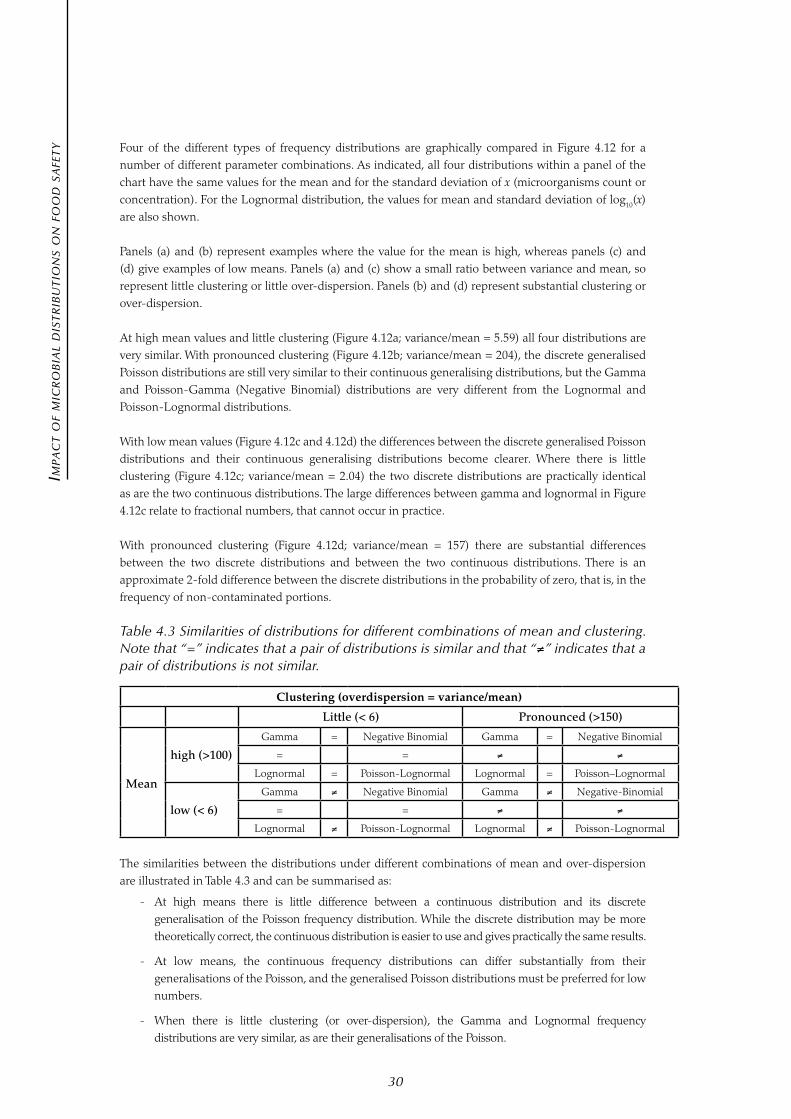
Imp

ac

t o

f m

Icr

ob

Ial

dIs

tr

Ibu

tIo

ns o

n f

oo

d s

afe

ty

30

Four of the different types of frequency distributions are graphically compared in Figure 4.12 for a number of different parameter combinations. As indicated, all four distributions within a panel of the chart have the same values for the mean and for the standard deviation of x (microorganisms count or concentration). For the Lognormal distribution, the values for mean and standard deviation of log10(x) are also shown.

Panels (a) and (b) represent examples where the value for the mean is high, whereas panels (c) and (d) give examples of low means. Panels (a) and (c) show a small ratio between variance and mean, so represent little clustering or little over-dispersion. Panels (b) and (d) represent substantial clustering or over-dispersion.

At high mean values and little clustering (Figure 4.12a; variance/mean = 5.59) all four distributions are very similar. With pronounced clustering (Figure 4.12b; variance/mean = 204), the discrete generalised Poisson distributions are still very similar to their continuous generalising distributions, but the Gamma and Poisson-Gamma (Negative Binomial) distributions are very different from the Lognormal and Poisson-Lognormal distributions.

With low mean values (Figure 4.12c and 4.12d) the differences between the discrete generalised Poisson distributions and their continuous generalising distributions become clearer. Where there is little clustering (Figure 4.12c; variance/mean = 2.04) the two discrete distributions are practically identical as are the two continuous distributions. The large differences between gamma and lognormal in Figure 4.12c relate to fractional numbers, that cannot occur in practice.

With pronounced clustering (Figure 4.12d; variance/mean = 157) there are substantial differences between the two discrete distributions and between the two continuous distributions. There is an approximate 2-fold difference between the discrete distributions in the probability of zero, that is, in the frequency of non-contaminated portions.

Table 4.3 Similarities of distributions for different combinations of mean and clustering. Note that “=” indicates that a pair of distributions is similar and that “≠” indicates that a pair of distributions is not similar.

Clustering (overdispersion = variance/mean)

Little (< 6) Pronounced (>150)

Mean

high (>100)

Gamma = Negative Binomial Gamma = Negative Binomial

= = ≠ ≠

Lognormal = Poisson-Lognormal Lognormal = Poisson–Lognormal

low (< 6)

Gamma ≠ Negative Binomial Gamma ≠ Negative-Binomial

= = ≠ ≠

Lognormal ≠ Poisson-Lognormal Lognormal ≠ Poisson-Lognormal

The similarities between the distributions under different combinations of mean and over-dispersion are illustrated in Table 4.3 and can be summarised as:

- At high means there is little difference between a continuous distribution and its discrete generalisation of the Poisson frequency distribution. While the discrete distribution may be more theoretically correct, the continuous distribution is easier to use and gives practically the same results.

- At low means, the continuous frequency distributions can differ substantially from their generalisations of the Poisson, and the generalised Poisson distributions must be preferred for low numbers.

- When there is little clustering (or over-dispersion), the Gamma and Lognormal frequency distributions are very similar, as are their generalisations of the Poisson.

Impa

ct o

f mIc

ro

bIa

l dIst

rIb

ut

Ion

s on fo

od s

afet

y

31

- In the presence of substantial clustering, the Gamma and Lognormal frequency distributions are substantially different, as are their generalisations of the Poisson.

The choice between the Gamma and Lognormal distributions or between their generalisations of the Poisson cannot be made solely on mathematical grounds and must depend on the basis of science and how well they fit actual observations. Table 4.4 summarises some of the literature concerning goodness of fit to observations.

At high levels there is substantial positive experience supporting the use of the Lognormal frequency distribution. However, the Gamma distribution has not been explored as an alternative, so the published experience does not really inform the choice.

At low levels of microorganisms, there is evidence of over-dispersion and superiority of the Poisson-Gamma (Negative Binomial) relative to the Poisson frequency distribution. Unfortunately, there has been very little reported use of the Poisson-Lognormal frequency distribution, perhaps because of the practical difficulties, so again the experience to date may not fully inform the choice of type of frequency distribution.

Table 4.4 Comparative fit of distributions to data; literature

Reference Material Distribution(s) considered

Comments

Greenwood

and Yule, 1917

Water Poisson - Reviewed by Elshaarawi et al., 1981

- Poisson appropriate for replicate water analyses

under carefully controlled conditions

- Negative binomial appropriate for samples collected

from different locations and over time

Fisher, 1941 Water Negative Binomial

Pipes et al.,

1977

Water Poisson

Negative Binomial

Lognormal

Gill et al., 1997 Hamburgers Lognormal - Substituted zero counts with an arbitrary value of

0.316 cfu/g (1/√10)

- Still substantial deviations from lognormal

Horowitz et al.,

1999

Ground beef Lognormal - No statistically significant deviation (Lilliefors test),

but small data sets and high means.

Gale et al., 1997 Raw water Poisson

Negative Binomial

- Reported by Gale, 2001

- Poisson fitted raw water, filtering increased dispersion

so Negative Binomial fitted better.

Gale, 2002 Water (treated) Poisson

Negative Binomial

- Statistically significant overdispersion when

compared to Poisson, Negative Binomial fitted better

Flores and

Stewart, 2004

Beef (artificially

contaminated)

Chi-squared

Lorentzian

Gauss-Lorentz cross

product

- Unusual distributions, not discrete and allow negative

values.

- Used to model levels (presence modelled separately)

Masago et al.,

2004

Water Poisson

Poisson-Lognormal

Negative Binomial

- Substantial overdispersion relative to Poisson

- Poisson-Lognormal fitted as well as Negative

Binomial

Gale, 2005 Raw burger

patties

Poisson

Lognormal

Poisson-Lognormal

- Used counts reported by Tuttle et al., 1999,

recalculated by Powell et al., 2000

- Overdispersion relative to Poisson

- Lognormal fitted to positive samples

- Negative samples interpreted as non-zero (below

limit of detection)

- Poisson-Lognormal used for risk estimation, not

fitted to data

Imp

ac

t o

f m

Icr

ob

Ial

dIs

tr

Ibu

tIo

ns o

n f

oo

d s

afe

ty

32

The importance of model choice, especially when choosing between a Gamma basis (including Negative Binomial) or a Lognormal basis (including Poisson-Lognormal), is much greater in the presence of substantial clustering.

Clustering can be quantified by the ratio variance/mean of the values (not the logs). Unfortunately, there are few reports in the literature that allow this ratio to be estimated from real data. Due to the popularity of the Lognormal distribution, it is unusual for the mean and variance (or standard deviation) of numbers to be reported. Almost invariably, statistics are reported for log(numbers) rather than for numbers.

Table 4.5 Literature values of the ratio variance/mean of organism numbers in water

Reference Microorganism; Material Variance/mean

Elshaarawi et al.,

1981

fecal streptococci; beach water 2.4, 12.0, 5.0

coliforms; lake water 42.1, 70.2, 19.8, 16.1, 18.9

Gale, 2002 Aerobe spores; raw water 1.1, 1.4, 1.5, 2.3, 2.4, 2.1, 2.8

Aerobe spores; treated water 6.4, 144.1, 64.4, 1146, 9.4, 10.7, 3.9, 144, 1.0, 2.1

Coliforms; raw & treated water 2.6, 1.2, 0.8, 1.3, 0.9, 1.0

Bacillus subtilis spores; raw water 1.0, 2.0, 2.7, 2.7, 2.5, 5.3, 2.3

B. subtilis spores; treated water 12.1, 3.1, 1.0, 1.1, 1.9, 3.2, 1.2, 2.1, 1.0, 7.0

Cryptospoidium parvum oocysts;

treated water

1.0, 1.0, 1.0, 1.0

Table 4.5 shows some values of the ratio for water. The data show that, even in water where a uniform random spatial distribution might be most likely, there is evidence for occasional substantial clustering.

As discussed earlier, mixtures of distributions are likely to occur frequently in practice. Despite this, there has been little direct investigation or description of such mixtures.

Some relevant literature is summarised in Table 4.6.

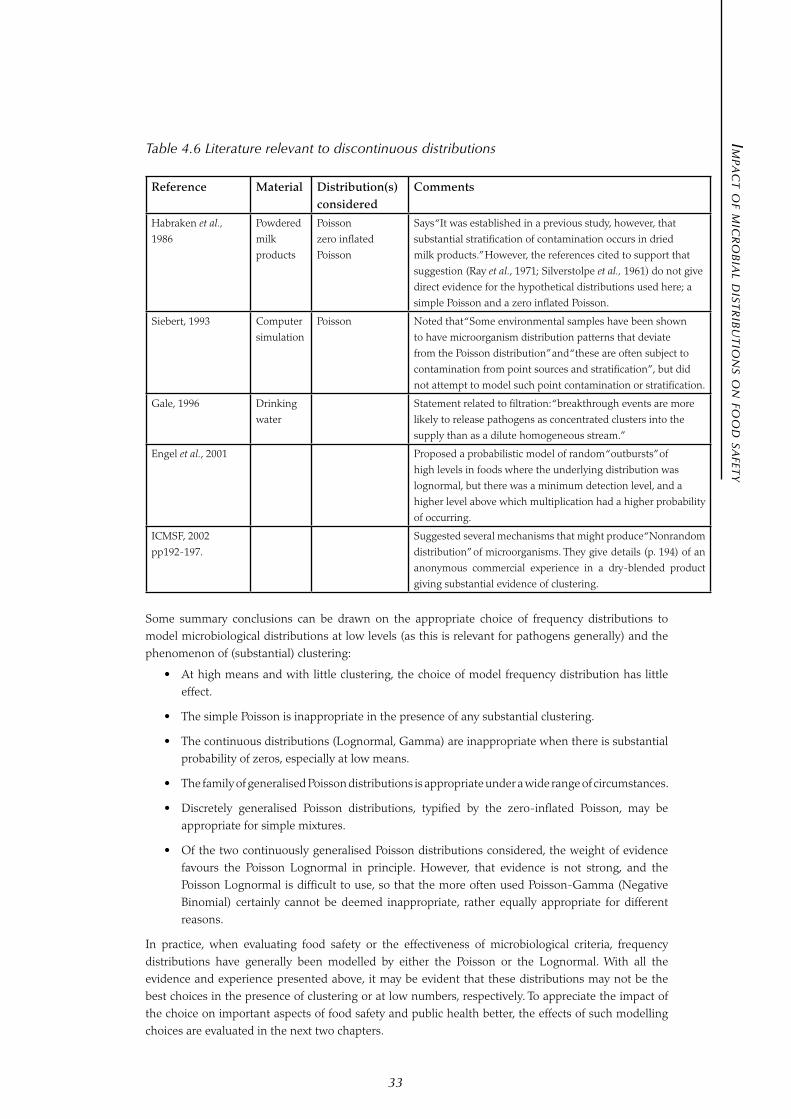
Impa

ct o

f mIc

ro

bIa

l dIst

rIb

ut

Ion

s on fo

od s

afet

y

33

Table 4.6 Literature relevant to discontinuous distributions

Reference Material Distribution(s) considered

Comments

Habraken et al.,

1986

Powdered

milk

products

Poisson

zero inflated

Poisson

Says “It was established in a previous study, however, that

substantial stratification of contamination occurs in dried

milk products.” However, the references cited to support that

suggestion (Ray et al., 1971; Silverstolpe et al., 1961) do not give

direct evidence for the hypothetical distributions used here; a

simple Poisson and a zero inflated Poisson.

Siebert, 1993 Computer

simulation

Poisson Noted that “Some environmental samples have been shown

to have microorganism distribution patterns that deviate

from the Poisson distribution” and “these are often subject to

contamination from point sources and stratification”, but did

not attempt to model such point contamination or stratification.

Gale, 1996 Drinking

water

Statement related to filtration: “breakthrough events are more

likely to release pathogens as concentrated clusters into the

supply than as a dilute homogeneous stream.”

Engel et al., 2001 Proposed a probabilistic model of random “outbursts” of

high levels in foods where the underlying distribution was

lognormal, but there was a minimum detection level, and a

higher level above which multiplication had a higher probability

of occurring.

ICMSF, 2002

pp192-197.

Suggested several mechanisms that might produce “Nonrandom

distribution” of microorganisms. They give details (p. 194) of an

anonymous commercial experience in a dry-blended product

giving substantial evidence of clustering.

Some summary conclusions can be drawn on the appropriate choice of frequency distributions to model microbiological distributions at low levels (as this is relevant for pathogens generally) and the phenomenon of (substantial) clustering:

• At high means and with little clustering, the choice of model frequency distribution has little effect.

• The simple Poisson is inappropriate in the presence of any substantial clustering.

• The continuous distributions (Lognormal, Gamma) are inappropriate when there is substantial probability of zeros, especially at low means.

• The family of generalised Poisson distributions is appropriate under a wide range of circumstances.

• Discretely generalised Poisson distributions, typified by the zero-inflated Poisson, may be appropriate for simple mixtures.

• Of the two continuously generalised Poisson distributions considered, the weight of evidence favours the Poisson Lognormal in principle. However, that evidence is not strong, and the Poisson Lognormal is difficult to use, so that the more often used Poisson-Gamma (Negative Binomial) certainly cannot be deemed inappropriate, rather equally appropriate for different reasons.

In practice, when evaluating food safety or the effectiveness of microbiological criteria, frequency distributions have generally been modelled by either the Poisson or the Lognormal. With all the evidence and experience presented above, it may be evident that these distributions may not be the best choices in the presence of clustering or at low numbers, respectively. To appreciate the impact of the choice on important aspects of food safety and public health better, the effects of such modelling choices are evaluated in the next two chapters.

Imp

ac

t o

f m

Icr

ob

Ial

dIs

tr

Ibu

tIo

ns o

n f

oo

d s

afe

ty

34

5. iMpACt of MiCrobiAl distributions on publiC heAlth: effeCt of Clustering And “tAils”

ot all servings of a food product contain equal numbers of microorganisms and not all microorganisms are equally hazardous. First, in order to investigate how this may affect the public health outcome of different microbial distributions related to

clustering, the impact of different degrees of clustering on cases of illness will be described in section 5.1, assuming a specific number for the dose of a contaminant per serving and making use of the dose-response relationship. Second, by combining frequency distributions with dose-response relationships, an evaluation will be made in section 5.2 of the parts of the frequency distributions that mainly determine public health. In section 5.3 this will be extended towards different statistical distributions with various degrees of clustering.

5.1 The effect of clustering

Three very different degrees of clustering of a contaminant in a batch of servings are investigated: a regular, a random and a very clustered contamination (Figure 5.1).

Assuming that each batch consists of 108 servings, with each serving being consumed by a different consumer, and that a batch is contaminated with a total of 108 bacterial cells, then three extreme distributions can be considered:

• A regular distribution, in which every serving contains exactly one cell.

• A random distribution of cells, meaning that some servings contain 0 cells, some 1, some 2 etc. as can be described by a Poisson distribution.

• A very clustered distribution, in which one serving contain all of the 108 cells as a cluster in a single serving and all the other servings are free of the contaminant.

Figure 5.1 Regular, random and very clustered distribution of a contaminant in a batch of servings; 20 servings out of the complete batch are shown as examples.

Regular Random Clustered

N

Impa

ct o

f mIc

ro

bIa

l dIst

rIb

ut

Ion

s on fo

od s

afet

y

35

While the level of clustering of a contaminant may affect the resulting illnesses in the population upon exposure, the number of illnesses likely also depends on how virulent the contaminating microogranism is and on its ability to proliferate in the product to reach higher levels.

Different scenarios related to virulence and growth potential of the hazard will be investigated, for each of the three types of clustering (see Table 5.1) with the batch of 108 servings, either considering no growth, 104-fold growth or 105-fold growth (hereafter referred to as 4-logs growth and 5-logs growth, respectively), with regard to their ultimate impact on the projected numbers of illness.

Seven different scenarios are investigated (see Table 5.2):

1. A microorganism with a relatively low virulence, for which the probability of illness can be described by the Binomial dose-response relationship with an r value of 1x10-10 cfu-1 (representing Listeria, Buchanan et al., 1997), and which does not grow in the product.

2. The same microorganism as in scenario 1, but additionally it is assumed that it can grow by four logs in the product.

3. A microorganism with a relatively high virulence, for which the probability of illness can be described by the Binomial dose-response relationship with an r value of 0.002 cfu-1 (representing Salmonella, FAO/WHO 2002), and which does not grow in the product.

4. The same microorganism as in scenario 3, but additionally it is assumed that it can grow by four logs in the product.

5. A toxin producing microorganisms, which will result in illness if the serving contains more than 105 microorganisms, and which does not grow in the product.

6. The same hazard as in scenario 5, but additionally it is assumed that it can grow by four logs in the product.

7. The same hazard as in scenario 5, but additionally it is assumed that it can grow by five logs in the product.

Table 5.1 Distributions of cells for different cases and growth stages

Growth Stage Case 1 Regular Case 2 Initially Random Case 3 Clustered

Initial:

mean 1 cell/

serving

Every serving

contains 1 cell

Single cells are Poisson (µ=1) distributed.

Cells/serving % servings

0 36.8%

1 36.8%

2 18.4%

3 6.13%

4 1.53%

5 0.31%

6 0.051% etc.

One in 108 servings

contains 108 cells.

Remaining servings have

no cells.

After 4 logs

growth:

mean 104 cells/

serving

Every serving

contains 104 cells

Cell clusters are Poisson distributed;

every cluster has 104 cells.

Cells/serving % servings

0 36.8%

104 36.8%

2x104 18.4%

3 x104 6.13%

4 x104 1.53%

5 x104 0.31%

6 x104 0.051% etc.

One in 108 servings

contains 1012 cells.

Remaining servings have

no cells.

Imp

ac

t o

f m

Icr

ob

Ial

dIs

tr

Ibu

tIo

ns o

n f

oo

d s

afe

ty

36

After 5 logs

growth: mean

105 cells/serving

Every serving

contains 105 cells

Cell clusters are Poisson distributed;

every cluster has 105 cells.

Cells/serving % servings

0 36.8%

105 36.8%

2x105 18.4%

3 x105 6.13%

4 x105 1.53%

5 x105 0.31%

6 x105 0.051% etc.

One in 108 servings

contains 1013 cells.

Remaining servings have

no cells.

Table 5.2 Illnesses per 108 servings, considering different microorganisms and scenarios with the Binomial dose-response model a,b

Scenario Growth stage Case 1Regular

Case 2Random

Case 3Clustered

low virulence; r = 10-10; Pr(ill|dose) = 1-(1-r)dose

1 Initial (mean 1 cell/serving) 0.01 0.01 0.00995

2 After 4 logs growth (mean 104 cells/serving) 100 100 1

high virulence r = 0.002; Pr(ill|dose) = 1-(1-r)dose

3 Initial (mean 1 cell/serving) 200000 199800 1

4 After 4 logs growth (mean 104 cells/serving) 100000000 63212056 1

Toxin producer causes illness at or above 105 cells

5 Initial (mean 1 cell/serving) 0 0 1

6 After 4 logs growth (mean 104 cells/serving) 0 11.14 1

7 After 5 logs growth (mean 105 cells/serving) 100000000 63212056 1

a If the number in the table is equal to or above one, it is the number of illnesses in the population; if the number is below 1, it is the probability that one consumer will become ill in the whole population (of 108 consumers consuming 108 servings).

b The Binomial dose-response model (Haas, 2002) is used, since the scenarios result in a specific known single dose, that is entered in the dose-response model to obtain the number of illnesses or probability of illness in one consumer.

Considering the single-value outcomes of the seven different scenarios, assuming an exact dose-response relationship, and the three degrees of clustering, the number of illnesses are calculated if these 108 servings are consumed. There is no significant effect of the clustering on the number of illnesses in the case of scenario 1; for all degrees of clustering the number of illnesses estimated is 0.01, meaning a probability of 1 in 100 that one illness will occur in the whole population. In scenario 2, with 4 logs of growth of the contaminant, the number of illnesses in the clustered case is 1, since all the contamination is in one serving. For the initially random and regular cases, many more illnesses are estimated, since in a higher proportion of the servings contamination is at a relatively high level. It should be noted that, due to the (localised) growth, now clustering is also obtained in the initially random case. While, servings initially free of microorganisms remain microorganisms free, servings that do contain microorganisms contain much higher levels after the projected 4 logs of growth.

In scenarios 3 and 4, a microbial hazard with higher infectivity than that in the previous 2 scenarios is evaluated. In the clustered case, for both scenarios, only the single contaminated serving results in one case of illness, but the random and regular cases show much higher numbers of cases of illness. Especially high numbers are estimated for scenario 4, as this considers 4 logs of growth of the contaminant. In scenario 4, for the regularly distributed contamination, it is predicted that all servings are contaminated and, thus, that all 108 consumers will get ill. In the initially random case 37% of the servings were not contaminated (due to randomness), so the number of illnesses in that case was projected as 6.3x107.

Impa

ct o

f mIc

ro

bIa

l dIst

rIb

ut

Ion

s on fo

od s

afet

y

37

In scenario 5, it is assumed that a toxin-former contaminated the product, which will cause illness if a serving contains more than 105 microorganisms. In the clustered case, only 1 illness will occur since all of the 108 cells of the contaminant are located in a single serving bringing the number of microorganisms in this serving above 105. The random and regular microbial distributions do not result in projected illnesses, since the numbers per serving are far below the levels necessary to surpass the threshold cell concentration for toxin production. In scenario 6, the toxin-former grows 4 logs, which in the regular case will not result in illness, because all servings will contain 104 microorganisms after growth, below the level necessary for toxicity. For the random distribution, there are a few products that initially contain more than 10 microorganisms (although on average there is 1), and these products will result finally in levels above 105 cells/serving. However, with 5 logs growth (scenario 7), also in regular contaminated servings and all initially-randomly contaminated products, the threshold cell level for toxin formation (105 cells/serving) is reached. Like in scenario 4, much higher numbers of illnesses result in scenario 7, with the maximum number of illnesses in the regular case (for the random case, again, 37% of the servings are not initially contaminated).

These scenarios show that clustering of pathogenic microorganisms can have an impact on public health. In most scenarios, a clustered contamination results in fewer illnesses than is the case for randomly or regularly distributed contaminations. If there is a certain level above which notable illness in the population occurs, as could be the case for toxin formers, in specific cases a clustered contamination can result in the numbers of illnesses being relatively higher than in the case of random or regular microbial distributions. In this case the example used the sequence is ‘bulk-package-growth’. Results will of course be different if the sequence were ‘bulk-growth-package’, since then the distribution over the packages would be carried out after the growth stage.

5.2 Effect of a frequency distribution of the exposure

In order to determine the effects on public health of frequency distributions of the dose per serving values within a batch of servings, it has to be combined with the dose-response relationship. Thus, the probability of illness for the whole exposure distribution is integrated. The exposure distribution for batches of product manufactured over time in multiple factories will be influenced by the between-factory variability, the between-batch variability, the within-batch variability and the variability due to a different storage history of the products. Therefore the mean concentration of a contaminant in a product will have a certain frequency distribution, P( ).

As a simple example, consider 5-litre containers of milk as the equivalent of batches. Each container holds many servings, say 100 mL each. Within each 5-litre container the microorganisms are randomly spread throughout the product, so the within-container distribution of concentration per serving (dose) is Poisson. However, the batch shows between-container variation in concentrations of the contaminant, which is assumed to be Lognormally distributed. In this example the within-container distribution of individual doses (Poisson) combines with the between-container distribution of means (Lognormal) to give a batch-wide distribution of individual doses that is Poisson-Lognormal. Such an example is explored in subsections 5.2.1, 5.2.2 and 5.2.3.

The number of illnesses in a population is the probability of illness multiplied by the number of servings consumed in the population (S). The probability of illnesses is the combined effect of the dose distribution (P(C )) and the dose-response relation (Pill) (see section 8.9):

Imp

ac

t o

f m

Icr

ob

Ial

dIs

tr

Ibu

tIo

ns o

n f

oo

d s

afe

ty

38

(1)

Nill: the number of illnesses in the population consuming S servingsS: the number of servings Pill : the probability of illness given exposure to a single dose from a Poisson distribution with mean

dose (the dose-response relation)D : the mean dose (number of microorganisms) in a group of servings within which the dose is

Poisson distributed with = MC : the mean concentration (cfu/g) in that group of servingsM: the serving size (g) P(C ): the probability that a serving comes from a group with mean

5.2.1 Example 1: listeria with relatively high levels

As an example we will show this approach for a product in which the mean concentration of Listeria monocytogenes within a batch of servings is Lognormally distributed (Figure 5.2a), with parameters log10(C )=Normal(0,2) and a serving size M=100g. The maximum dose per serving is 1x1010 cfu, since the maximum level of L. monocytogenes is assumed to be 1x108 cfu/g -1 and the serving size is 100g. This results in a mean-dose distribution of log10( )=Normal(2,2). So the mean-concentration and mean-dose within the batch are Lognormally distributed, meaning that the log10(C ) and log10(D ) are normally distributed.

For this distribution the geometric mean for the concentration is 1 cfu/g and for the dose 100 cfu. Due to the bigger relative impact of the right-hand tail of the Lognormal distribution, the arithmetic mean is 40287 cfu/g (log10(C ) = 4.605) for the concentration and 4.03x106 cfu for the dose (see Textbox).

Incidentally, if the distribution of doses within each batch is Poisson, the overall distributions of concentration and dose in individual servings across different batches are Poisson-Lognormally distributed.

This dose distribution can be combined with the exponential dose-response relationship, with an r-value (representing Listeria) of 1x10-10 cfu-1 (Buchanan et al., 1997) (Figure 5.2b). In contrast to section 5.1, where the Binomial dose-response model is used to calculate cases of illness, here the exponential dose-response model is used, since now it concerns the probability of illness from a single dose (as part of a dose distribution of exposure) with mean dose , so the unconditional dose-response (Haas, 2002).

Integrating these two curves results in a combined frequency of illness given a certain dose, combining both its impact and its frequency of occurrence (Figure 5.2c).

Impa

ct o

f mIc

ro

bIa

l dIst

rIb

ut

Ion

s on fo

od s

afet

y

39

Figure 5.2

a)

b)

c)

a) Frequency distribution of Log normally distributed mean dose of Listeria log10( )=Normal (2,2) (with x-axis on a log scale). This represents the probability that a random dose comes from a group with the given mean.

b) Exponential dose-response relation r=1x10-10 cfu-1. This represents the probability that a random dose from a Poisson distributed group of doses with the given mean causes illness.

c) Graph a and b combined to determine the overall frequency of illness (in a similar appraoch as Stellbrink and Dahms 2004).

This example can be represented in equation 1 as:

(2)

This integral can be calculated to be 1x10-4, meaning a risk per serving of 1 in 10000. If, for example, a million people each consume 100 servings in a year, S = 100 million servings would be consumed and this would result in 10000 cases. It should be realized that this number of predicted cases would be reduced if the prevalence of contamination were taken into account. For example, if the prevalence is of the order of 10%, and, furthermore, the susceptible group is not the whole population but only 20% of the population, the resulting number of cases would be estimated as 200.

Figure 5.2 shows the relationship between exposure and resulting illnesses. Figure 5.2a depicts the frequency distribution of the mean dose and Figure 5.2b shows the probability that a dose causes illness. Mathematically combining exposure (a) with dose-response (b) details, results in the frequency distribution of illness for various doses shown in Figure 5.2c. From Figure 5.2c, the likely number of illnesses caused by a specific dose can be seen. Comparing it with Figure 5.2a (the dose distribution), one can conclude that the largest number of illnesses is caused by the very infrequent but very high doses. In other words, the right hand tail of the exposure distribution largely determines the cases of illness. It should be recognised that the x-axis reflects the dose on a log-scale; thus, going one unit to the right increases the dose by a factor 10 and as a consequence also the probability of illness is increased by a factor of 10.

Imp

ac

t o

f m

Icr

ob

Ial

dIs

tr

Ibu

tIo

ns o

n f

oo

d s

afe

ty

40

5.2.2 Example 2: listeria with lower levels

If a concentration distribution of log10( )=Normal(-4,2) is used with a serving size of M=100 g, the dose will be distributed as log10( )=Normal(-2,2). This will result in 3.6 cases per 100 million servings or 3.6 cases per million people per year, each consuming 100 servings in a year. The data are graphically shown in Fig. 5.3.a-c. The conclusion reached for the data in Figure 5.2, that the very low prevalent high doses are substantially determining risk, also holds true here.

Figure 5.3

a)

b)

c)

a) Frequency distribution of Log normally distributed mean dose of Listeria log10( )=Normal ( 2,2) (with x-axis on a log scale) ).

b) Exponential dose-response relation with r=1x10-10 cfu-1.

c) Graph a) and b) combined to determine the overall frequency of illness.

In other risk assessments as well, the final probability of illness is in many cases largely determined by the extreme doses, despite these doses being very infrequent, because they result in a much higher probability of illness.

While the main region that determines the ultimate risk to consumers in these calculations is found to be the right hand extremes, it should be noted that the confidence in the accuracy of the frequency distribution function in these regions is very limited.

The calculations until now are all based on the dose at consumption. Infrequent high doses at the moment of consumption are the main determining risk. It should be realized that these high doses at the moment of consumption can result from infrequent high levels earlier in the chain, but also from a low concentration earlier in the chain with abuse conditions during the product’s shelf-life.

Impa

ct o

f mIc

ro

bIa

l dIst

rIb

ut

Ion

s on fo

od s

afet

y

41

5.2.3 Example 3: salmonella with low levels

Salmonella is used in further calculations aimed at establishing the relationship between variability in dose, dose-response and ultimate level of illness (Figure 5.4). Assuming a higher infectivity, the dose-response relationship for Salmonella saturates at lower doses than for Listeria. This is shown in Figure 5.4b, where the probability of illness reaches a plateau at Pill = 1. Compare Figure 5.3b with 5.4b and note that the dose-response relationship has moved to the left.

The calculations regarding the graphs of illness caused by Salmonella are based on an r value of 0.002 cfu-1 and a log mean dose distribution of Normal (-6,2). The overall estimated level of illness is 3500 cases per 100 million servings (or 3500 cases per million people per year, that consume on average 100 servings per year). In this case also, the doses mainly responsible for illness are from the right hand tail of the dose distribution. Figure 5.4 a)

b)

c)

a) Frequency distribution of Log normally distributed mean dose of Salmonella log10( )=Normal (-6,2) (with x-axis on a log scale).

b) Exponential dose-response relation (Exp) with r=0.002 cfu-1 and beta-Poisson model (BP) with parameters alpha = 0.1324 and beta = 51.45.

c) Graph a) and b) combined to determine the overall frequency of illness.

Of course, if another dose-response model is used, other results will be obtained quantitatively. For example, if we take the Beta-Poisson model:

and make use of the parameters alpha=0.1324 and beta =51.45 (FAO/WHO 2002), the result is a different dose-response relationship (see Figure 5.4b). However, the effect on the number of illnesses (3089 per million people in contrast to 3500 for the Binomial model) and the range of doses that are responsible for the cases remains similar (Figure 5.4c).

Imp

ac

t o

f m

Icr

ob

Ial

dIs

tr

Ibu

tIo

ns o

n f

oo

d s

afe

ty

42

The number of cases results mainly from servings with log10 doses between -2 and +2 in the range where the two models do not deviate greatly. The model used to describe the doses in a serving for the calculations in the above examples for Listeria and Salmonella (subsections 5.2.1, 5.2.2 and 5.2.3) actually is a Poisson-Lognormal distribution of doses.

5.3 Comparison of the effects of various distributions and various degrees of clustering We can now evaluate the effects of various distributions and of various degrees of clustering (with a higher degree of clustering being equivalent to increased standard deviation) on the overall risks to consumers. To illustrate this, we can take an example similar to that in subsection 5.2.1 above, with a (geometric) mean (log10( )) of Listeria of 2.0, but with the standard deviation (log ) varying from 0.2 to 2.0. These values are realistic for concentrations in contaminated food products with a standard deviation of 0.2 representing a rather unclustered contamination, and a standard deviation of 2 a relatively clustered contamination. For illustration purposes, the resulting values for log10 of the mean ( ) and standard deviation ( ) are shown in the first and second columns of Table 5.3. The within-group Poisson distribution results in a Poisson-Lognormal (PLN) distribution of individual doses with resulting illness rates (column PLN). The Poisson-Lognormal distribution represents a clustered distribution of microorganisms, in which the extent of clustering is indicated by the sd2/mean ratio shown in Table 5.3. For comparison, Table 5.3 also includes the illness rates calculated for the Negative Binomial (column NB) distribution and an un-clustered Poisson distribution with the same mean dose (column Poisson). These illness rates are calculated making use of Monte-Carlo simulations.

Table 5.3 listeria risk calculations for three dose distributions with a fixed (geometric) mean(log10( ))=2.0 and increasing standard deviations.

Dose distribution parameters Equivalent Lognormal parameters

log10 (illness rates) from different dose distributions

log10

( )

log10

(sd( ))

log10

sd²/mean

Mean

(log10( ))

sd

(log10( ))

Poisson

log(Pill)

PLNa

log(Pill)

NBb

log(Pill)

2.05 1.74 1.44 2 0.2 -7.95 -7.95 -7.95

2.18 2.25 2.31 2 0.4 -7.82 -7.82 -7.82

2.41 2.79 3.17 2 0.6 -7.59 -7.59 -7.59

2.74 3.47 4.20 2 0.8 -7.26 -7.26 -7.26

3.15 4.30 5.45 2 1 -6.85 -6.85 -6.85

3.66 5.32 6.97 2 1.2 -6.34 -6.34 -6.34

4.26 6.51 8.77 2 1.4 -5.74 -5.75 -5.76

4.95 7.89 10.84 2 1.6 -5.05 -5.11 -6.02

5.73 9.46 13.19 2 1.8 -4.27 -4.51 -7.56

6.61 11.21 15.82 2 2.0 -3.39 -4.00 -9.31

a Poisson Log Normal, b Negative Binomial

From this table it can be concluded that all three statistical distributions (Poisson, PLN, NB) give comparable results for deviations (sd) up to 1.4. For higher standard deviations, the Negative Binomial distribution gives results that strongly deviate from the other two distributions, which remain more comparable.

All individual types of distributions show that the risk, in terms of probability of illness, increases substantially with increasing standard deviation (which equates to a higher degree of clustering).

Impa

ct o

f mIc

ro

bIa

l dIst

rIb

ut

Ion

s on fo

od s

afet

y

43

Notably, this increase in risk relates to the increase in arithmetic mean that is concomitant with the increase in standard deviation. In other words, although the geometric mean in the example has been fixed to 2, with larger standard deviations the value of the arithmetic mean increases more than proportionally.

In order to investigate this effect further, the same type of calculations are carried out with an arithmetic mean fixed at 500 (log10 = 2.70) and changing arithmetic standard deviation (sd).

Table 5.4 listeria calculations for three dose distributions with a fixed arithmetic mean (=500) and increased standard deviations.

Dose distribution parameters Equivalent Lognormal parameters

log10(Illness rates) from different dose distributions

log10

( )

log10

(sd( ))

log10

sd²/mean

Mean

(log10( ))

sd

(log10( ))

Poisson

log(Pill)

PLNa

log(Pill)

NBb log(Pill)

2.70 1.5 0.30 2.70 0.02 -7.30 -7.30 -7.30

2.70 2.0 1.30 2.69 0.08 -7.30 -7.30 -7.30

2.70 2.5 2.30 2.63 0.25 -7.30 -7.30 -7.30

2.70 3.0 3.30 2.35 0.55 -7.30 -7.30 -7.30

2.70 3.5 4.30 1.89 0.84 -7.30 -7.30 -7.30

2.70 4.0 5.30 1.40 1.06 -7.30 -7.30 -7.30

2.70 4.5 6.30 0.90 1.25 -7.30 -7.30 -7.30

2.70 5.0 7.30 0.40 1.41 -7.30 -7.30 -7.30

2.70 5.5 8.30 -0.10 1.56 -7.30 -7.30 -7.31

2.70 6.0 9.30 -0.60 1.69 -7.30 -7.31 -7.34

a Poisson Log Normal, b Negative Binomial

As is apparent from Table 5.4, in most cases the risk is equal and where there are differences in the estimated risk they are marginal. Thus, neither the choice of the statistical distribution nor the standard deviation has an impact on the overall level of risk for a specific value of the arithmetic mean. In Table 5.5, the above example for Listeria is re-calculated for Salmonella, characterised by a higher virulence as compared to Listeria, taking r = 0.002, the arithmetic mean fixed at dose = 0.1 (log10 = -1) and a range of increased arithmetic standard deviations.

Table 5.5 salmonella risk calculations for three dose distributions with a fixed arithmetic mean dose D =0.1 and increased standard deviations.

Dose distribution parameters Equivalent Lognormal parameters

log10(Illness rates) from different dose distributions

log10

( )

log10

(sd( )

log10

sd²/mean

Mean

(log10( ))

sd

(log10( )

Poisson

log(Pill)

PLNa

log(Pill)

NBb

log(Pill)

-1 0.5 2.00 -2.50 1.14 -3.70 -3.72 -3.74

-1 1.0 3.00 -3.00 1.32 -3.70 -3.75 -3.96

-1 1.5 4.00 -3.50 1.47 -3.70 -3.79 -4.52

-1 2.0 5.00 -4.00 1.61 -3.70 -3.86 -5.28

-1 2.5 6.00 -4.50 1.74 -3.70 -3.93 -6.12

-1 3.0 7.00 -5.00 1.86 -3.70 -4.02 -7.00

-1 3.5 8.00 -5.50 1.98 -3.70 -4.11 -7.91

-1 4.0 9.00 -6.00 2.08 -3.70 -4.21 -8.84

-1 4.5 10.0 -6.50 2.19 -3.70 -4.32 -9.78

-1 5.0 11.0 -7.00 2.28 -3.70 -4.43 -10.76

a Poisson Log Normal, b Negative Binomial

Imp

ac

t o

f m

Icr

ob

Ial

dIs

tr

Ibu

tIo

ns o

n f

oo

d s

afe

ty

44

Because of the higher virulence, the probability of illness for Salmonella is estimated to be much higher than in the example with Listeria. However, again, the risks calculated with the Poisson and Poisson-Lognormal frequency distributions are very similar, and markedly different from those calculated with the Binomial distribution. For the Poisson-Lognormal, there is a slight decrease in risk with increasing standard deviation. Considering, however, the relatively substantial uncertainties normally associated with quantitative calculations of risk, this decrease could be considered to be a minor effect. The Negative Binomial distribution gives results, which are quite different from those obtained with the other two types of frequency distributions, and shows a gradual decrease in the level of risk with an increase in the standard deviation. In this case, it is evident that the choice of the frequency distribution does influence the calculated risk outcome. Therefore, there is a real need to substantiate the selection of the dose distribution using actual distribution data and selecting the best-fitting model.

5.4 Conclusion

In many cases the choice of the distribution does not have a large impact on the estimated risk and it is the arithmetic mean that is a major descriptor of the overall risk level. In certain situations, however, the choice of the distribution impacts significantly on the magnitude of the risk. Therefore, it is relevant to have a good understanding of a situation or to have concrete data at hand that can help decide which type of distribution is the most appropriate (valid) in particular situations.

Impa

ct o

f mIc

ro

bIa

l dIst

rIb

ut

Ion

s on fo

od s

afet

y

45

6. iMpACt of MiCrobiAl distributions on perforMAnCe objeCtives And MiCrobiologiCAl CriteriA

ow that the impact of the choice of the frequency distribution on an estimated public health risk has been investigated, the next step is to evaluate its impact on the setting of performance objectives and microbiological criteria.

6.1 Performance Objectives

A Performance Objective (PO) is defined as ‘the maximum frequency and/or concentration of a hazard in a food at a specified step in the food chain before the time of consumption that provides or contributes to a ‘food safety objective’ (FSO)5 or an ‘appropriate level of protection’ (ALOP), as applicable’ (CAC, 2007).

The PO and FSO concepts are rather new in international food safety management. Few, if any, POs (or FSOs or ALOPs) have been authoritatively defined, so their content remains a subject for speculation. Some standards may appear to have features of a PO or FSO. For example, the EU Scientific Committee on Veterinary Measures Relating to Public Health (EC, 1999) recommended:

‘An objective must be to keep the concentration of L. monocytogenes in food below 100 cfu/g and to reduce the fraction of foods with a concentration above 100 L. monocytogenes per gram significantly.’

This is not an FSO because 100 cfu/g is not a strict maximum valid for all portions of a food product or batch thereof, but rather a ‘target for improvement’, for which the fraction of foods above the stated level is to be reduced. Indeed, the recommendation continues ‘This objective should be expressed as a Food Safety Objective’ clarifying that, as it stands, the proposed objective is not a Food Safety Objective.

A PO set by a competent authority is justified in terms of public health protection as it relates to an ALOP. Accordingly, to the extent that the public health impact of microorganisms depends upon their distribution in a food as well as on their number (as discussed in chapter 5 above), both aspects should be considered when setting a PO. In this regard, the choice of the type of frequency distribution is important and should best reflect understanding of important aspects of distribution, such as homogeneity or heterogeneity. If, in the relevant circumstances, clustering of the microogranism in the products concerned is likely, it may have a marked impact on the risk in the population. Then, an objective for risk reduction should consider clustering as part of risk-reduction measures or of standards, such as a Performance Objective. In fact, to be effective in these circumstances, a PO may need to be more sophisticated than a simple limit on ‘the maximum frequency and/or concentration’. A recent discussion (Rieu et al., 2007) supports the view that FSOs should be framed with due regard to dose frequency distributions, and suggests a mathematical framework within which this might be accomplished. Also the recent paper by van Schothorst et al. (2009) discusses FSOs, POs and microbiological criteria, and the relationship between them in the context of risk-based food safety management.

N

5. FSO, Food Safety Objective. A PO set at the time of consumption. Definition: The maximum frequency and/or concentration of a hazard in a food at the time of consumption that provides or contributes to the appropriate level of protection (ALOP). (CAC, 2007)

Imp

ac

t o

f m

Icr

ob

Ial

dIs

tr

Ibu

tIo

ns o

n f

oo

d s

afe

ty

46

6.2 Microbiological Criteria

While the information to be included in a Food Safety or Performance Objective is not very clear, a Microbiological Criterion is well-defined (CEC, 2005). It is ‘the acceptability of a product, a batch of foodstuffs or a process, based on the absence or presence or number of microorganisms … per unit(s) of mass, volume, area, or batch’ and includes:

• Microbiological limits

• The number of portions which should conform to those limits

• A sampling plan defining the number of ‘field samples’ to be taken and the size of the ‘analytical unit’.

This explicitly includes details of the size and number of portions considered, so that the effect of the known/assumed distribution of the microorganisms on the performance of the microbiological criterion can be assessed.

The phrase ‘acceptability of ... a batch ... based on ... microorganisms … per unit(s) ... batch’ implies that the acceptability of a batch can be expressed in terms of a single value; the average or total number of microorganisms. However, previous sections have indicated that differing distributions can lead to differences in microbiological status even when total numbers remain the same, and that this can lead to differences in risk. Differing spatial distributions are sometimes discussed as ‘within-lot’ and ‘between-lot’ distributions, but previous sections have shown that spatial distributions can be more subtle than implied by such a dichotomy.

On the basis of the microbiological criterion, the acceptability of a batch (or a product or a process) can be assessed from a limited sample. However, even if microorganisms are distributed in a uniform random manner throughout a batch, sampling variation means the sample will not perfectly represent the whole, leading to variable outcomes, especially at very low concentrations.

For example, if a batch of 100,000 chocolate bars is contaminated with 1000 Salmonella (and no individual bar contains more than one microorganism), then 1000 bars are contaminated. A random sample of one bar then has only 1% chance of detecting Salmonella. In other words, there is 99% chance that a sample of one bar will fail to detect Salmonella at 1% prevalence of contaminated bars. If the number of bars in the sample is increased, the chance of failing to detect the contamination is less. However, even with a sample of 60 bars there is 0.9960 = 55% chance that none will contain Salmonella. If the spatial distribution of microorganisms is clustered, then there may be fewer than 1% of bars contaminated, as contamination per bar may be by multiple cells, and there may be a much higher chance of failing to detect any of the 1000 Salmonella.

The limitations of sampling in detecting low levels of contamination and especially as a means to ensuring safety are well-recognised in authoritative regional and international guidance. For example:

• ‘The safety of foodstuffs is mainly ensured by a preventive approach, such as implementation of good hygiene practice and application of procedures based on hazard analysis and critical control point (HACCP) principles’ (CEC, 2005).

• ‘The microbiological safety of food is principally ensured by selection of raw materials, control at the source, product design and process control, and the application of HACCP during production, processing, distribution, storage, sale, preparation, and use. This comprehensive preventive system offers much more control than end-product testing.’ (International Commission on Microbiological Specifications for Foods, ICMSF, 2002).

Impa

ct o

f mIc

ro

bIa

l dIst

rIb

ut

Ion

s on fo

od s

afet

y

47

The value of sampling lies in supporting other safety assurance systems – ‘Microbiological criteria can be used in validation and verification of HACCP procedures and other hygiene control measures’ (CEC, 2005) – and in putting pressure on the producer to maintain high standards – ‘The producer must see that the product is of high quality, otherwise there will be inconvenience and expense with unacceptable lots’ (ISO, 2006).

Whatever the distribution of microorganisms, the ability of a sample to distinguish between batches of different quality or safety depends on both the within-batch variability and the between-batch variability. In Figure 6.1 each curve illustrates the variation within a single batch; thus, the different curves represent between-batch variation. In Figure 6.1a, there is substantial overlap between adjacent batches (means differing by 1.0 unit) so that it would be difficult to assign any particular value to any particular batch quality, but there is little overlap between extreme batches (means differing by 4.0). In Figure 6.1b, there is the same within-batch variation but smaller between-batch variation, so that it would be difficult to distinguish even extreme batches. In Figures 6.1c and d, the within-batch variation has been reduced by a factor of 5, so that even adjacent batches in the widely spaced group (c) can be distinguished, and for the closely spaced batches (d) the extremes have little overlap. Figure 6.1 Within- and between-batch variability. Different curves represent different batches.

If the within-batch variability is small compared to between-batch variability (Figure 6.1c), a relatively small sample can give a good indication of the quality of a batch in comparison to other batches. If the within-batch variability is large in comparison to the between-batch variability (Figure 6.1b), a limited size sample is largely uninformative. When the within-batch and between-batch variabilities are comparable (Figure 6.1a and d) a limited size sample can only distinguish grossly different batches.

As generally implemented (e.g., CEC, 2005) microbiological criteria are ‘attributes sampling plans’ as described by Dahms, 2004.

Imp

ac

t o

f m

Icr

ob

Ial

dIs

tr

Ibu

tIo

ns o

n f

oo

d s

afe

ty

48

6.3 Attributes sampling plans

In the context of this work a sampling plan is fully defined by four numbers; n, c, m, M where: n is the number of portions examined to determine the acceptability of the batch,

c is the maximum acceptable number of portions with values above m

but no portions are acceptable with values above M.

n and c are numbers of portions, m and M are values to which test results on a portion may be compared. For a two-class plan, M is indefinitely large. For a presence/absence plan, m is zero (in an analytical portion).

NB: These definitions are applicable whether the values of m and M are continuous values, such as concentrations, or integer discrete values, such as numbers of cfu.

The effectiveness of a sampling plan is described by its ‘operating characteristic’, which gives the probability of a batch meeting the criterion as a function of the quality of the batch (Figure 6.2). By convention, operating characteristics are drawn with batch quality decreasing to the right and probability of the sample(s) meeting the criteria increasing upwards. The operating characteristic shows that there is a probability – ideally small – that a high quality batch will be rejected (A in Figure 6.2) or a low quality batch will be accepted (B in Figure 6.2); these probabilities are sometimes known as Producer’s (or Seller’s) and Consumer’s (or Buyer’s) Risks, respectively.

Figure 6.2 Diagrammatic representation of Operating Characteristic

Assuming that the distributions of the values in the n portions are identical and independent, the probability of batch acceptance is as shown in the footnote6. A graphical plot of acceptance probability against batch quality is an operating characteristic (such as Figure 6.2 above). The batch quality is defined by the values of the portions in the batch, F(x|…) in the footnote. This is just the frequency distribution function discussed in chapter 4 above.

6.

where: B() is the binomial cumulative distribution functionF(x|…) is the cumulative frequency distribution function of unit values, the probability that the value is no more than x given the distribution parameters (represented as …)

Impa

ct o

f mIc

ro

bIa

l dIst

rIb

ut

Ion

s on fo

od s

afet

y

49

In the general application of acceptance sampling plans (e.g., BSI, 2005; Grant and Leavenworth, 1996), the spatial distribution is often taken as uniform random leading to a Poisson (or sometimes Binomial) frequency distribution, defined by one parameter, so that batch quality is defined by one parameter: the mean. As outlined in chapter 4 above, when considering microbiological contamination of foods and possible clustering, the dispersion is also important, so that other parameters as well as the mean, must be considered when assessing batch quality and calculating acceptance probabilities.

Scientists, who considered the impact of microbiological frequency distributions on sampling plan performance (Dahms, 2004 and Legan et al., 2001), used a Lognormal distribution of microogranism numbers in their studies. Legan et al. (2001) demonstrated the dependence of acceptance probability on standard deviation (see their Figure 5) and Dahms (2004) remarked that ‘the effect of using an attributes plan is also dependent on the validity of the underlying assumptions for the frequency distribution, especially with regard to its standard deviation’.

However, generally, both Legan et al. (2001) and Dahms (2004) demonstrated the general dependence of acceptance probability on the mean with an assumed standard deviation of 0.8 log10 units.

The graph presented by Legan et al. (2001; their Figure 5) suggests that changing the standard deviation from about 0.1 to 3.0 log10 units decreases the mean concentration of microorganisms giving a 5% probability of acceptance by about 4 log10 cycles. Figure 6.3 shows operating characteristics against the mean with the same sampling plan and range of standard deviations used by Legan et al. (2001). It confirms that changing the standard deviation of a Lognormal distribution can completely change the performance of a sampling plan. Figure 6.3 Dependence of acceptance probability on variability (Lognormal distribution)

Neither Legan et al. (2001) nor Dahms (2004) discussed the impact of other forms of frequency distribution. However, as depicted in Figure 6.4, which shows operating characteristics against mean for five different types of frequency distributions, the impact is substantial. In this figure, the arithmetic variances of the different distributions are equal and fixed at 1000 (except for the Poisson where the variance equals the mean). The microbiological criterion in this example sampling plan is ‘absent in the portion’ for any of 5 samples taken. This has a natural interpretation for the discrete distributions (i.e., the Poisson, Negative Binomial and Poisson-Lognormal distributions) but needs some elaboration for the continuous distributions (i.e., Gamma and Lognormal), where the variable is concentration in the sample (cfu/portion) rather than count and where there is zero probability of 0 cfu/portion. Following the practice of Dahms (2004), Legan et al. (2001) and others, ‘absent in the portion’ has been interpreted as ‘<1 cfu/portion’ for the continuous distributions.

Imp

ac

t o

f m

Icr

ob

Ial

dIs

tr

Ibu

tIo

ns o

n f

oo

d s

afe

ty

50

Figure 6.4 Dependence of acceptance probability on form of frequency distribution in the case of large over-dispersion (equivalent to substantial clustering)

The operating characteristics for different distributions are similar in shape, but are separated from each other. The differences are quite substantial, as indicated by the selected values shown in Table 6.1.

Table 6.1 Selected values from Figure 6.4: The case of large overdispersion

Lognormal Gamma Poisson Poisson Lognormal

Negative Binomial

mean cfu for

Pr(accept) =

5% 5.0 12 0.60 3.7 11.5

50% 1.4 5.5 0.14 0.77 5.1

95% 0.11 1.3 0.01 0.05 1.2

Pr(accept) at mean = 1 cfu 61% 97% 0.7% 42% 97%

Even neglecting the Poisson, whose variance is substantially less than the other distributions, there are substantial differences between the operating characteristics based on the different distributions; the difference between the three discrete distributions is especially striking, as is the similarity between the Gamma and the Negative Binomial.

In Figure 6.4, the ‘important’ part of the operating characteristics can be thought of as those where the acceptance probability is changing rapidly, that is, where the mean is less than about 10. At this mean, the chosen variance of 1000 (except for the Poisson where the variance equals the mean) suggests substantial clustering. The variance value of 1000 was chosen arbitrarily on the basis that, for a mean of around 5 cfu, the Lognormal distribution gives a standard deviation of log10 values of about 0.8, which is the standard deviation generally used (Dahms, 2004; ICMSF, 2002; Legan et al., 2001). Choosing an arithmetic variance of 10 (representing much less clustering), as was done for Figure 6.5 (except for the Poisson; note the selected values listed in Table 6.2), results in significantly smaller differences between operating characteristics corresponding to different frequency distributions.

Impa

ct o

f mIc

ro

bIa

l dIst

rIb

ut

Ion

s on fo

od s

afet

y

51

Figure 6.5 Dependence of acceptance probability on type of frequency distribution in the case of little over-dispersion (indicating little clustering)

Table 6.2 Selected values from Figure 6.5

Lognormal Gamma Poisson Poisson Lognormal

Negative Binomial

Mean cfu for

Pr(accept) =

5% 1.8 2.0 0.60 1.3 1.6

50% 0.65 0.81 0.14 0.32 0.68

95% 0.07 0.16 0.01 0.02 0.14

Pr(accept) at mean = 1 cfu 28% 38% 0.7% 9.8% 28%

As expected from section 4.5, the difference between the Poisson Lognormal and the Negative Binomial is smaller when the degree of clustering (over-dispersion) is smaller.

In summary:

• Clustering, as evidenced by a change in the standard deviation for a constant mean, has a critical effect on the acceptance probability for typical microbiological criteria.

• The choice of frequency distributions used to model microbial distributions has a substantial effect on the evaluation of microbiological criteria.

Imp

ac

t o

f m

Icr

ob

Ial

dIs

tr

Ibu

tIo

ns o

n f

oo

d s

afe

ty

52

7. disCussion, ConClusions And reCoMMendAtions

7.1 Discussion

Microorganisms associated with food are subject to intense study in an effort to reduce the numbers of pathogenic microorganisms that are ingested in any serving and to reduce the level of illness in the population. However, the physical distributions of these microorganisms are rarely considered, perhaps due to the variety of processes at work, the potential complexity of the outcomes, and the very heavy experimental load to characterise distributions.

In this report, we looked at mechanisms that have an impact on physical distributions, characteristics of frequency distributions employed to model microbial distributions, and the impact of both physical and frequency distributions on illness risk and food safety management criteria.

We outlined six mechanisms that can impact the microbial distribution in a foodstuff: contamination, growth, death, joining, mixing, and fractionation. The impact of each of these mechanisms is relatively easy to predict qualitatively in terms of the degree of clustering of microorganisms, and can be predicted quantitatively. However, the complexity is increased by the fact that it is more common to have a number of different mechanisms, in concert or in series that can influence the final outcome. The level of clustering will vary depending on, for instance, materials, processes and conditions. Clustering leads to increased variation in the values of doses, i.e., increased standard deviation (sd) of frequency distribution, statistically called over-dispersion.

In the absence of data on actual physical distributions of microorganisms in food, our review examined the more common frequency distributions used for modelling real situations, and evaluated their strengths and weaknesses. Furthermore, we considered the impact of choosing one frequency distribution over another.

To assist the risk assessor or risk manager in choosing a frequency distribution to be used in risk assessment or in the application of microbiological criteria (MC) and acceptance sampling plans, we have outlined five desirable characteristics:

• It should be non-negative, as it is not possible to have negative numbers of microorganisms.

• It should allow zeros, as it is possible to have no microorganisms in a portion.

• It should be discrete, as it is not possible to have partial microorganisms in a portion.

• It should reduce to (or approximate) the Poisson, as the frequency distribution corresponding to perfectly uniform spatial distributions (perfect mixing).

• It should approximate the Lognormal at high numbers, as this distribution, which can model microbiological ‘tails’, has empirical support.

Although Poisson frequency distributions may be a workable approximation depending on the situation, clustering makes their use less appropriate. While it is not possible to make firm recommendations on the most appropriate frequency distribution for each specific circumstance, one of the family of generalised Poisson frequency distributions is likely to be most suitable. The Poisson-Lognormal distribution is preferred on theoretical grounds; however, it is difficult to apply in practice. The more often used Poisson-Gamma (Negative Binomial) is also appropriate and easier to apply.

The choice of frequency distribution will generally be between the Poisson where there is good mixing, the Lognormal distribution for large numbers and the Poisson-Lognormal or Negative Binomial distribution in other circumstances.

Impa

ct o

f mIc

ro

bIa

l dIst

rIb

ut

Ion

s on fo

od s

afet

y

53

The continuous distributions (Lognormal, Gamma) are inappropriate when there is a substantial probability of zeros, especially at low means. When the mean is high, there is little difference between frequency distributions, regardless of clustering.

Ultimately the final choice is not just a statistical one, but one that fits the data best. Familiarity and ease of use will also influence the choice of a model frequency distribution.

We have shown that risk can be heavily influenced by variability in doses, as caused by clustering, as well as average dose. Data is not available to assess the nature and degree of this effect in reality, but we do know that often the risk is largely determined by infrequent high doses, the right hand tail of the frequency distribution. These infrequent high values are the most important contributors to the arithmetic mean in a batch and thus it is the arithmetic mean (mean of counts), which is more relevant to the assessment of risk than the geometric mean (mean of logs).

Because clustering can affect the consumer risk, it is a phenomenon that also needs to be considered in the establishment of food safety management targets such as Performance Objectives (PO). However, we are not yet able to conclude, in more detail, how best to consider clustering.

A PO is described as a ‘maximum frequency and/or concentration’ at a particular point in the food chain. In cases where clustering is known or shown to be relevant, this definition may not cover the phenomenon. In any case, it is important that a PO is established with due consideration of which dose frequency distribution to choose, as different distributions may lead to different interpretations of what the ‘maximum’ limit for frequency and/or concentration would be in specific scenarios.

Clustering also has a significant impact on the acceptance probability for typical MCs and the effectiveness of sampling. This impact is due to the influence of clustering on the standard deviation of the dose frequency distribution and on the nature of the distribution itself.

Even if microorganisms exhibit an almost regular distribution in a batch of food, negative test results do not prove absence, but merely reflect the effect of sampling probability. This is especially true for the very low concentrations at which such microorganisms would be encountered in practice. When the spatial distribution of microorganisms is more clustered, the chance of failing to detect contamination may be even higher.

The within-batch variability and the between-batch variability have an impact on the effectiveness of sampling. If the within-batch variability is very small and the between-batch variability very large, a small number of samples will give a good indication of the quality of a batch in comparison to other batches. If the within-batch variability is, however, very large, in comparison to the between-batch variability, the same number of samples is much less informative.

Clearly, the physical distribution of microorganisms in a foodstuff, as well as the frequency distributions with which we choose to model these distributions, are important in the field of risk assessment and risk management. This is true in the evaluation of risk and in the setting of microbiological criteria and food safety management targets. We make many assumptions when undertaking these activities, some more critical than others. Criticality will depend on the specific activity and particular situation under consideration.

7.2 Conclusions

• Understanding the distribution or combinations of distributions of microorganisms arising from the various mechanisms involved in the processing of food is important. However, there is a lack of objective, quantitative evidence on the nature of these distributions.

Imp

ac

t o

f m

Icr

ob

Ial

dIs

tr

Ibu

tIo

ns o

n f

oo

d s

afe

ty

54

• In order to evaluate the degree of clustering that actually happens in a food system and to be able to make a determination of which frequency distributions are appropriate, data are needed from multiple quantitative measurements of individual batches.

• The choice of frequency distribution will be guided by data fit and influenced by ease of use; the Poisson-Lognormal is an appropriate choice theoretically but difficult to work with in practice. The Poisson is appropriate where there is good mixing, the lognormal distribution for large numbers and the Poisson-Lognormal or Negative Binomial distribution in other circumstances.

• Risk assessors should take into account the effect of clustering on variability of dose. When information on variability is not available, so that risk assessment must be based only on average dose, the arithmetic mean (mean of counts) is more appropriate than the geometric mean (mean of logs), although the latter is more generally available. This conclusion is consistent with others working in the field of quantitative risk assessment.

• A more sophisticated definition of PO that includes consideration of clustering might be needed. As it is not possible to define a true maximum and the arithmetic mean is the major determinant of risk, linking food safety management targets to the arithmetic mean may be more appropriate than setting a maximum limit

• Regulatory risk managers assessing the effectiveness of MCs should be aware of the typical standard deviations for products of interest, and promote the incorporation of various standard deviations into tables of sampling plans. Awareness of the importance of the choice of frequency distributions used to model microbial distributions is also required when evaluating microbiological criteria.

• The within-batch variability and the between-batch variability also have to be taken into account to determine the effectiveness of sampling.

• It is important that risk assessors and risk managers are aware of which assumptions have the greatest impact on their particular situation and seek clarity on that situation to inform their choices.

7.3 Recommendations

In this report we have made some recommendations that may assist risk assessors and risk managers with their choices of frequency distribution.

• Better insight into the physical distributions that arise from the mechanisms affecting the spatial distribution of microorganisms is needed, through thorough microbiological evaluation of multiple individual batches of different products.

• The data generated should be quantitative rather than presence/absence only.

• When reporting data, both the mean and standard deviation of the numbers should be reported as well as the log10 (numbers).

• While the Poisson-Lognormal has a number of theoretical advantages, its complexity makes it a difficult choice for risk assessors and further development and understanding of the mathematics of this distribution would be useful.

• Finally, we recommend published evaluation of different or new approaches to utilising the various distributions in risk assessments and to setting risk management targets or microbiological criteria that could overcome some of the limitations inherent in our present-day assumptions.

Impa

ct o

f mIc

ro

bIa

l dIst

rIb

ut

Ion

s on fo

od s

afet

y

55

8. MAtheMAtiCAl Annex

his annex collects some information on mathematical aspects, presented with little explanation, but will hopefully be useful to mathematicians working in this area.

Sections 8.1 to 8.6 define some frequency distributions in terms of their probability density functions (for continuous distributions) or probability mass functions (for discrete distributions) and give some properties including the mean and variance (sd2).

Section 8.7 gives relationships between parameters of different distributions with the same moments (mean and variance).

Section 8.8 briefly describes the principles of Monte Carlo modelling, which may be used to combine frequency distributions and other functions.

Section 8.9 describes some models for relationships between dose and probability of illness.

8.1 Normal distribution

mean(x) = median(x) = mode(x) = µsd2(x) = σ2

8.2 Lognormal distribution

sd2(ln(x)) = σ2median(x) = exp(ξ); mode(x) = exp(ξ - σ2)

In the context of microbiology, where x are microorganism levels and log10 is often preferred to ln, this leads to the following relationship between the log of the means and the mean of the logs (see Rahman, 1968, pp 298-299) in which the log of the means is higher than the mean of the logs by an amount proportional to the variation in logs. log10(mean(x)) = mean(log10(x)) + sd2(log10(x)).ln(10)/2

T

Imp

ac

t o

f m

Icr

ob

Ial

dIs

tr

Ibu

tIo

ns o

n f

oo

d s

afe

ty

56

8.3 Gamma distribution

8.4 Poisson distribution

mean(x) = sd2(x) = λmode(x) = int(λ) [also = λ-1 if λ is integer]

8.5 Negative Binomial distribution

This is often taken as relating to a sequence of Binomial (fail/succeed) trials (probability of success = p). Under that interpretation it can be taken as modelling either: a) the number of trials before a specified number (k) of successes or

b) the number of failures before a specified (k) number of successes.

Here we use the latter parameterisation

In other interpretations k need not be integer, in which case

Impa

ct o

f mIc

ro

bIa

l dIst

rIb

ut

Ion

s on fo

od s

afet

y

57

8.6 Poisson-Lognormal distribution

8.7 Converting between distributions

When comparing the five types of frequency distributions considered in this report, we wish to choose parameter values making the distributions as similar as possible. Here we interpret ‘similar’ as having equal mean and (except for the Poisson) equal variance leading to the relationships in this table. Each row holds equations for the parameters of that distribution in terms of the parameters of the distributions in each column. The first row and column (A) show the mean and variance of the variate.

Imp

ac

t o

f m

Icr

ob

Ial

dIs

tr

Ibu

tIo

ns o

n f

oo

d s

afe

ty

58

† In all non-trivial circumstances, the Negative Binomial and the Poisson-Lognormal are over-dispersed with respect to the Poisson, their variance exceeds their mean. Accordingly, these pairs of relationships cannot be satisfied simultaneously (except trivially by setting λ = 0 or σp = 0).

Impa

ct o

f mIc

ro

bIa

l dIst

rIb

ut

Ion

s on fo

od s

afet

y

59

8.8 Monte Carlo modelling

The discussions in this report often concerned the combination of different distributions with each other and with other functions, for example:

• Generalised Poisson distributions, as described in chapter 4, involved combinations of a Poisson and a generalising distribution.

• Assessment of public health impact, as described in chapter 5, involved combination of frequency distributions for levels with dose-response functions.

• Assessment of sampling plans, as described in chapter 6, involved combination of frequency distributions for levels with functions of sampling plan parameters.

In addition, it is often necessary to integrate distributions and other functions, e.g., to evaluate the proportion below a value, rather than the relative frequency at the value. In some cases this can be done ‘analytically’, that is, by manipulation of the relevant equations to give an explicit equation for the result. For example, a combination of the Gamma probability density function (pdf, section 8.3) with the Poisson pdf (section 8.4) gives the Negative Binomial pdf (section 8.5). When feasible, this is the preferred approach. Sometimes, however, analytical evaluation is not practical; for example, it is not possible to analytically integrate the Normal pdf (section 8.1) to give its cdf. In such cases one alternative is to use Monte Carlo modelling, which is a computer-based technique allowing variation in randomly distributed ‘inputs’ to be propagated and combined through mathematical models allowing observation of consequent variation in outputs. Although the technique can be implemented in many forms, the most feasible approach for non specialists is to use an add-in to Microsoft Excel, of which the most widely used are @Risk (Palisade Corporation, 2004) and Crystal Ball (Decisioneering, 2005).

The first stage is to create a deterministic7 spreadsheet model that encapsulates the input-output relationships, without considering variability. Each input is represented by a single typical value. Formulae in spreadsheet cells represent the input-output relationships for each step, so that the final cells produce the results corresponding to the typical input values. The deterministic model can be used to calculate the outcomes corresponding to any given set of input values. The next stage is to replace each of the variable inputs – single valued in the deterministic model – with an appropriate frequency distribution. This figure (Figure 8.1) shows a hypothetical deterministic model as a solid curved line; it has only one input and one output, but the principles remain the same for more complicated models. Each input value has exactly one corresponding output value, as shown by the dashed lines and arrows. The variability associated with the input is represented as a Normal distribution, above the graph. The principle of Monte Carlo modelling is to randomly sample a number of input values from that distribution to calculate the resulting output distribution, shown on the right of the graph. As illustrated, output distributions can be very different from input distributions. The computer automatically generates many random scenarios from the input distributions, collecting corresponding outputs. One scenario (a set of input values) and its corresponding set of output values is known as an ‘iteration’. The complete collection of iterations is known as a ‘simulation’.

Figure 8.1

7. In this context “deterministic” means the opposite of “stochastic”, that there is no variability or uncertainty.

Imp

ac

t o

f m

Icr

ob

Ial

dIs

tr

Ibu

tIo

ns o

n f

oo

d s

afe

ty

60

8.9 Impact of microbial distributions and dose-response on public health

8.9.1 Illness per servingThe relation between the probability to get ill and the ingested dose can be represented with a Binomial dose-response model: (A1)

with Pill: the probability of illness given an exposure to Dose DD: dose of microorganisms (number of microorganisms) r: the dose-response parameter (per number of microorganisms).

This equation can be seen as that in order to have no illness, for all microorganisms in the dose, no illness results. For dose = 1 the probability of illness equals r, the probability of no illness equals 1-r. For dose D the probability of no illness equals (1-r)D, so none of the microorganisms in the dose D does provoke illness. So finally the probability of illness equals 1-(1-r)D. If the dose is assumed to have been sampled from a homogenous food product with an average dose , this Poisson sampling process will result in the exponential model:

(A1b)

Practically, these two equations will result in approximately equal results.

The number of microorganisms is given as cfu both in the case of concentrations, where it is relevant, as in the case of doses where it should be more considered as the number of infective units. It should be realized that a ‘Dose’ can only be 1, 2, 3 or any positive integer-number of microorganisms, but an expected dose can also be 1.2 or 0.1 microorganisms.

8.9.2 Illness in a populationIf a population, for example 1 million people, consume together S servings with an expected dose , the number of illnesses will be:

(A2)

with Nill: the number of illnesses in the population consuming S servingsS: the number of servings The expected number of illnesses (Nill) can be for example 10 or 25, but can also be smaller than 1, for example 0.1. In this case Nill, should be considered more as a probability of one person in a population of 1 million individuals to get ill.

Furthermore, it is important that in this equation we multiply the probability per serving (Pill) by the number of servings, acknowledging that, in principle, one person can get ill twice a year, and that this then is counted as 2 illnesses, while also accepting that immunity could reduce the probability of a second infection. Counting 2 illnesses thus would be an overestimation of the number of illnesses. On the other hand, it could also be the case that, as a result of the first infection, a person may be even more susceptible to a second infection, due to a weaker health status.

Impa

ct o

f mIc

ro

bIa

l dIst

rIb

ut

Ion

s on fo

od s

afet

y

61

8.9.3 Including variable dosesIn reality not all doses will be equal, since both the concentration of microorganisms (C) and the serving size (M) will differ in every serving, therefore equation A2 can also be seen as:

(A3)

In words: each Dose , has a probability of illness (equation A1b), so the total number of illnesses is the sum of the respective probability of illness in every serving i over all servings.

By using the expected concentration ( ) multiplied by the serving size (M) for the Dose, = .M, this results in: (A4)

with i: the expected concentration of microorganisms in serving i (cfu/g)Mi: the serving size of serving i (g)r: the dose response parameter (cfu-1)

Often the concentration will vary over various orders of magnitude, while the mass per serving will change within roughly a factor of 10. So we will focus mainly on concentration distribution, but the variability in serving sizes can also be included in the calculations.

8.9.4 Continuous concentration distributionsConsidering that very large amounts of food products are generally consumed by a population of, for instance, 1 million people and that the concentration then can be considered as a continuous distribution, equation A4 can also be written as:

(A5)

with P( ) the frequency of average concentration , given a certain concentration distribution of the microorganism in the products. This equation can be read as: the number of illnesses equals the number of servings, multiplied by the integration of the probability to encounter a certain average concentration, P( ), with the probability to become ill given that average concentration, Pill( ).

This equation also holds for other dose response equations (for example the Beta-Poisson model). In general this could be represented as:

(A6).

Imp

ac

t o

f m

Icr

ob

Ial

dIs

tr

Ibu

tIo

ns o

n f

oo

d s

afe

ty

62

9. referenCes

BSI (British Standards Institution), (2005). Guide to the selection and usage of acceptance sampling systems for inspection of discrete items in lots BS 6000. Part 1: General guide to acceptance sampling.

Buchanan, R.L., Damert, W.G., Whiting, R.C. and van Schothorst, M. (1997). Use of epidemiological and food survey data to estimate a purposefully conservative dose-reponse relationship for Listeria monocytogenes levels and incidence of Listeriosis. Journal of Food Protection 60:918-922.

CAC (Codex Alimentarius Commission), (2007). Procedural Manual 17th edition, Joint FAO/WHO Standards Programme, ISSN 1020-8070.

CEC (Commission of the European Communities), (2005). Commission Regulation (EC) No 2073/2005 on microbiological criteria for foodstuffs.

Dahms, S. (2004). Microbiological sampling plans – statistical aspects. Mitteilungen aus Lebensmittel-untersuchung und Hygiene 95:32-44.

Decisioneering (2005). Crystal Ball. Version 7.2. Decisioneering (UK) Ltd., London, UK.

EC, (1999). Opinion of the Scientific Committee on Veterinary Measures Relating to Public Health on Listeria monocytogenes. Available at: http://ec.europa.eu/food/fs/sc/scv/out25_en.pdf.

Elshaarawi, A.H., Esterby, S.R. and Dutka, B.J. (1981). Bacterial density in water determined by Poisson or negative binomial distributions. Applied and Environmental Microbiology 41:107-116.

Engel, R., Normand, M.D., Horowitz, J. and Peleg, M. (2001). A qualitative probabilistic model of microbial outbursts in foods. Journal of the Science of Food and Agriculture 81:1250-1262.

FAO/WHO, (2002). Risk assessments of Salmonella in eggs and broiler chickens. Microbiological Risk Assessment Series, no 2. ISSN 1726-5274.

Available at: ftp://ftp.fao.org/docrep/fao/005/y4392e/y4392e00.pdf

FAO/WHO, (2006). The use of microbiological risk assessment outputs to develop practical risk management strategies: metrics to improve food safety. Report of a joint FAO/WHO meeting. Available at: ftp://ftp.fao.org/ag/agn/food/kiel_en.pdf

Fisher, R.A. (1941). The negative binomial distribution. Annals of Eugenics 11:182-187.

Flores, R.A. and Stewart, T.E. (2004). Empirical distribution models for Escherichia coli O157:H7 in ground beef produced by a mid-size commercial grinder. Journal of Food Science 69: M121-M126.

Gale, P. (1996). Developments in microbiological risk assessment models for drinking water – a short review. Journal of Applied Bacteriology 81:403-410.

Gale, P. (2001). Developments in microbiological risk assessment for drinking water. Journal of Applied Microbiology 91:191-205.

Gale, P. (2002). The effect of drinking water treatment on the spatial heterogeneity of microorganisms: implications for assessment of treatment efficiency and health risk. Water-Research 36:1640-1648.

Impa

ct o

f mIc

ro

bIa

l dIst

rIb

ut

Ion

s on fo

od s

afet

y

63

Gale, P. (2005). Matrix effects, non-uniform reduction and dispersion in risk assessment for Escherichia coli O157. Journal of Applied Microbiology 99:259-270.

Gale, P., van Dijk, P.A.H. and Stanfield, G. (1997). Drinking water treatment increases microogranism clustering: the implications for microbiological risk assessment. Journal of Water Supply Research and Technology – Aqua 46:117-126.

Gill, C.O., Rahn, K., Sloan, K. and McMullen, L.M. (1997). Assessment of the hygienic performances of hamburger patty production processes. International Journal of Food Microbiology 36:171-178.

Grant, E. L. and Leavenworth, R. S. (1996). Statistical Quality Control. McGraw-Hill, New York.

Greenwood, M. and Yule, G.U. (1917). On the statistical interpretation of some bacteriological methods employed in water analysis. Journal of Hygiene 16:36-54.

Haas, C.N. (2002). Conditional dose-response relationships for microorganisms: development and application. Risk Analysis 22:455-463.

Habraken, C.J.M., Mossel, D.A.A. and van den Reek, S. (1986). Management of Salmonella risks in the production of powdered milk products. Netherlands Milk and Dairy Journal 40:99-116.

Horowitz, J., Normand, M. and Peleg, M. (1999). On modelling the irregular fluctuations in microbial counts. Critical Reviews in Food Science and Nutrition 39:503-517.

ICMSF (International Commission on Microbiological Specifications for Foods), (2002). Microorganisms in Foods 7: Microbiological Testing in Food Safety Management. Kluwer Academic/Plenum Publishers, New York.

ISO (International Organization for Standardization) (2006). ISO 2859-10 Sampling procedures for inspection by attributes – part 10: Introduction to the ISO 2859 series of standards for sampling for inspection by attributes.

Kilsby, D.C. and Pugh, M.E. (1981). The relevance of the distribution of microorganisms within batches of food to the control of microbiological hazards from foods. Journal of Applied Bacteriology 51: 345-354.

Legan, J.D., Vandeven, M.H., Dahms, S. and Cole, M.B. (2001). Determining the concentration of microorganisms controlled by attributes sampling plans. Food Control 12:137-147.

Masago, Y., Oguma, K., Katayama, H., Hirata, T. and Ohgaki, S. (2004). Cryptosporidium monitoring system at a water treatment plant, based on waterborne risk assessment. Water Science and Technology 50:293-299.

Nauta, M.J. (2001). A modular process risk model structure for quantitative microbiological risk assessment and its application in an exposure assessment of Bacillus cereus in a REPFED. RIVM Rapport 149106007.

http://www.rivm.nl/bibliotheek/rapporten/149106007.pdf

Nauta, M.J. 2005. Microbiological risk assessment models for partitioning and mixing during food handling. International Journal of Food Microbiology 100:311-322.

Palisade Corporation (2004). @Risk Version 4.5.3 - Industrial edition, Spittlefields, London, UK.

Imp

ac

t o

f m

Icr

ob

Ial

dIs

tr

Ibu

tIo

ns o

n f

oo

d s

afe

ty

64

Pipes, W.O., Ward, P. and Ahn, S.H. (1977). Frequency distributions for coliform bacteria in water. Journal of American Waterworks Association 69:664-668.

Powell, M.R., Ebel, E., Schlosser, W., Wladerhaug, M. and Kause, J.R. (2000). Dose-response envelope for Escherichia coli O157:H7. Quantitative Microbiology 2:141-163.

Rahman, N.A. (1968). A course in theoretical statistics. Charles Griffin & Co., London.

Ray, B., Jezeski, J.J. and Busta, F.F. (1971). Isolation of salmonellae from naturally contaminated dried milk products. 1. Influence of sampling procedure on the isolation of salmonellae. Journal of Milk and Food Technology 34:389-393.

Rieu, E., Duhem, K., Vindel, E. and Sanaa, M. (2007). Food safety objectives should integrate the variability of the concentration of pathogen. Risk Analysis 27:373-386.

Siebert, K.J. (1993). Computer-simulation of microbiological sampling of liquid foods. Journal of Food Protection 56:518-524.

Silverstolpe, L., Plazikowski, U., Kjellander, J. and Vahlne, G. (1961). An epidemic among infants caused by Salmonella muenchen. Journal of Applied Bacteriology 24:134-142.

Soanes, C. (2003). Compact Oxford English dictionary of current English. Oxford University Press, Oxford, UK.

Stellbrink E, Dahms S (2004). Dose-response-models and their implications for quantitative risk assessment for Campylobacter infections (in German). Berliner Und Munchener Tierarztliche Wochenschrift 117: 207-213.

Stoodley, P., Wilson, S., Hall-Stoodley, L., Boyle, D.J., Lappin-Scott, H.M. and Costerton, J.S. (2001), Growth and detachment of cell clusters from mature mixed-species biofilm. Applied and Environmental Microbiology 67: 5608-5613.

Stoyan, D. and Stoyan, H. (1994). Fractals, random shapes, and point fields: methods of geometrical statistics. Wiley, New York.

Tuttle, J., Gomez, T., Doyle, M.P., Wells, J.G., Zhao, T., Tauxe, R.V. and Griffin, P.M. (1999). Lessons from a large outbreak of Escherichia coli O157:H7 infections: insights into the infectious dose and method of widespread contamination of hamburger patties. Epidemiology and Infection 122:185-192.

van Schothorst, M., Zwietering, M.H., Ross, T., Buchanan, R.L. and Cole, M.B. (2009). International Commission on Microbiological Specifications for Foods (ICMSF). Relating microbiological criteria to food safety objectives and performance objectives. Food Control 20: 967-979.

other ilsi europe publications

Concise Monographs• Alcohol – health Issues related to Alcohol consumption• A simple guide to understanding and Applying the hazard

Analysis critical control point concept• calcium in nutrition• carbohydrates: nutritional and health Aspects• caries preventive strategies• concepts of functional foods• dietary fibre• food Allergy• food biotechnology – An Introduction• functional foods – from science to health and claims• genetic Modification technology and food – consumer health

and safety• healthy lifestyles – nutrition and physical Activity• Microwave ovens• nutrition and genetics – Mapping Individual health• nutrition and Immunity in Man• nutritional and health Aspects of sugars – evaluation of new

findings• nutritional epidemiology, possibilities and limitations• oral and dental health – prevention of dental caries, erosion,

gingivitis and periodontitis • oxidants, Antioxidants, and disease prevention• principles of risk Assessment of food and drinking Water

related to human health• the Acceptable daily Intake – A tool for ensuring food safety• threshold of toxicological concern (ttc)• type 2 diabetes – prevention and Management

reports• Addition of nutrients to food: nutritional and safety

considerations• An evaluation of the budget Method for screening food

Additive Intake• Animal-borne viruses of relevance to the food Industry• Antioxidants: scientific basis, regulatory Aspects and Industry

perspectives• Applicability of the AdI to Infants and children• Application of the Margin of exposure Approach to compounds in food which are both genotoxic and

carcinogenic• Approach to the control of entero-haemorrhagic Escherichia

coli (ehec)• Assessing and controlling Industrial Impacts on the Aquatic

environment with reference to food processing• Assessing health risks from environmental exposure to

chemicals: the example of drinking Water• campylobacters as Zoonotic pathogens: A food production

perspective• considering Water Quality for use in the food Industry• consumer understanding of health claims• detection Methods for novel foods derived from genetically

Modified organisms• emerging technologies for efficacy demonstration• exposure from food contact Materials• foodborne protozoan parasites• foodborne viruses: An emerging problem• food consumption and packaging usage factors• food safety Management tools• food safety objectives – role in Microbiological food safety

Management

• functional foods in europe – International developments in science and health claims

• functional foods – scientific and global perspectives• guidance for the safety Assessment of botanicals and botanical

preparations for use in food and food supplements• Markers of oxidative damage and Antioxidant protection:

current status and relevance to disease• 3-Mcpd esters in food products• Method development in relation to regulatory requirements

for the detection of gMos in the food chain• Micronutrient landscape of europe: comparison of Intakes and

Methodologies with particular regard to higher consumption• Mycobacterium avium subsp. paratuberculosis (MAp) and the

food chain• nutrition in children and Adolescents in europe: What is the

scientific basis?• overview of the health Issues related to Alcohol consumption• overweight and obesity in european children and

Adolescents: causes and consequences – prevention and treatment

• packaging Materials: 1. polyethylene terephthalate (pet) for food packaging Applications

• packaging Materials: 2. polystyrene for food packaging Applications

• packaging Materials: 3. polypropylene as a packaging Material for foods and beverages

• packaging Materials: 4. polyethylene for food packaging Applications

• packaging Materials: 5. polyvinyl chloride (pvc) for food packaging Applications

• packaging Materials: 6. paper and board for food packaging Applications

• packaging Materials: 7. Metal packaging for foodstuffs• recontamination as a source of pathogens in processed foods

– A literature review• recycling of plastics for food contact use• safety Assessment of viable genetically Modified Micro-

organisms used in food• safety considerations of dnA in foods• Salmonella typhimurium definitive type (dt) 104:

A multi-resistant Salmonella• significance of excursions of Intake above the Acceptable daily

Intake (AdI)• the safety Assessment of novel foods• the safety Assessment of novel foods and concepts to

determine their safety in use• threshold of toxicological concern for chemical substances

present in the diet• transmissible spongiform encephalopathy as a Zoonotic

disease• trichothecenes with a special focus on don• using Microbiological risk Assessment (MrA) in food safety

Management• validation and verification of hAccp

to order IlsI europe a.i.s.b.l. Avenue e. Mounier, 83, box 6 b-1200 brussels belgium phone: (+32) 2 771 00 14 fax: (+32) 2 762 00 44 e-mail: publications@ilsieurope.be

IlsI europe’s concise Monographs and report series can be downloaded from: http://www.ilsi.org/europe

Isbn 9789078637202