impact of government expenditure, exchange rate and

Global Business and Management Research: An International Journal

Vol. 13, No. 2 (2021)

14

Impact of Government Expenditure, Exchange Rate

and Unemployment Rate on Economic Growth of

Malaysia

Tiong Ing Ngiik, Jerome Kueh*, Josephine Yau, and Audrey Liwan

Faculty of Economic and Business, Universiti Malaysia Sarawak, 94300 Kota Samarahan,

Sarawak, Malaysia

Email Address: [email protected]

*Corresponding author

Abstract

The objective of the study is to investigate the association between government expenditure,

exchange rate and unemployment rate on economic growth of Malaysia from 1988 to 2017.

All variables in the model are cointegrated with two cointegrating vectors and implies that

long-run relationship exist. Granger Causality based on Vector Error Correction Model

(VECM) revealed an unidirectional short run causality from government expenditure to

economic growth, economic growth to unemployment, unemployment to exchange rate and

unemployment to government expenditure. Policies such as fiscal policy and exchange rate

policy need to be implemented by policy makers in Malaysia to ensure empowering economic

growth.

Keywords: Economic growth, exchange rate, government expenditure, Malaysia,

unemployment rate

Introduction

Major change in worldwide financial structure matters where globalization, advancement,

government strategies of countries will have significant global impact. According to World

Bank (2017), reports by Malaysia Economic Monitor, Malaysia’s growth accelerated to 2017,

development conjecture of 5.8%, which is the nation’s most astounding yearly development

rate from 2014 then relied upon to stay powerful at 5.2% in 2018. However, accelerated growth

is affected by increased domestic demand, enhanced labour market circumstances, wage

advancement, and enhanced external demand for made goods and product export in Malaysia.

The use of capital expenditures has further expanded due to an increase in private and public

investment. According to Abas (2017), reports by New Straits Times, the third quarter of 2017,

Malaysian economic development is the fastest in the Asia region. Malaysia leads Indonesia,

Taiwan, Singapore and so on. A nation’s economy grows at quicker rate during third quarter

of 2017 (6.2%) in contrast with 4.3% in similar period in 2016. Domestic demand continues to

grow, external sector improves, service sectors economic growth, manufacturing sectors and

agriculture sectors.

mailto:[email protected]


Vol. 13, No. 2 (2021)

15

(Sources: World Bank data 2020)

Figure 1: Economic Growth of Malaysia from 1988 to 2019

Figure 1 shows the economic growth of Malaysia from year 1988 to 2019. In year 1998, the

economic growth rate decreased sharply from 7.31% in 1997 to -7.34% in 1998. This is because

of the regional financial crisis on the Malaysian economy was felt in 1998. However, the

economic growth rate bounced back from -7.34% in 1998 to 8.86% in 2000. This is due to the

real output increased strongly by 10%, and the second half of the year maintained a strong

growth of 7.2%. Exports of manufactured goods also rose by 19.1% in the first half of the year

due to increased export (12.9%) and prices (5.5%). This export strength is due to the continued

strong demand for electronic and electrical products and the substantial expansion of oil-based

exports such as petroleum and chemical products. However, by the end of 2000, the global

economy began to slow down. This has an adverse effect on exports, especially

semiconductors.

However, Malaysia's economic growth decreased again from 8.86% in 2000 to 0.52% in 2001.

The economy stayed versatile during 2001 because of face challenges from the outside

condition. Slowdown of the global economic will affect export performance, which will also

affect the imports of goods and services for fare creation. In the year 2007, Malaysia had the

highest economic growth rate, which is 9.43%. The robust development accomplished reflects

the advantages of the progressively various financial base, which enhances the capacity of

economy to withstand external conditions. In an environment of declining external demand,

domestic demand, particularly in the private sector, prompted economic growth in 2007.

Domestic market developed unequivocally to 10.5% during 2007 compared to 2006 by 7%,

mainly due to the booming private consumption and investment. Buyer expenditure increase is

also maintained by stable growth in discretionary income, firm work advertises and positive

funding circumstances. Private investment invested activity remains powerful with larger

capital expenditures in industrial, serving and structure sectors. Simultaneously, the public

sector continues to support growth after implementing plans and actions to strengthen

framework and community area conveyance systems. In the year 2009, the Malaysia economy

shrank by -2.53%, a worldwide economy that encountered the worst depression in present day

history. The domestic economy experienced this circumstance in the first quarter of the

worldwide financial recession, a full-scale influence, down 6.2%, making the first year of real

GDP since the third quarter withdrawal in the fourth quarter in 2001. Global demand and the

(10.00)

(8.00)

(6.00)

(4.00)

(2.00)

-

2.00

4.00

6.00

8.00

10.00

12.00

19

91

19

92

19

93

19

94

19

95

19

96

19

97

19

98

19

99

20

00

20

01

20

02

20

03

20

04

20

05

20

06

20

07

20

08

20

09

20

10

20

11

20

12

20

13

20

14

20

15

20

16

20

17

20

18

20

19

Eco

no

mic

Gro

wth

Rat

e (

%)

Year


Vol. 13, No. 2 (2021)

16

fall of global exchange have prompted a twofold digit to decrease Malaysia’s export and

mechanical production. The specific economy is exceptionally turned on. External interest

deterioration affects engagement, salary and business, and consumer confidence, leading to a

decrease in private consumption and private investment activities this year during the first

quarter. The development quarter of the period was likewise influenced by the decline in large

inventories, especially in the manufacturing and commodity sectors. The economic growth in

2018 and 2019 portrayed growth at average 4.74% and 4.33%, respectively. In a nutshell, the

trend of economic growth of Malaysia from year 1988 to year 2019 is decreasing.


Figure 2: Government Expenditure and Economic Growth of Malaysia

Figure 2 shows the association between government expenditure and economic growth of

Malaysia from 1988 to 2019. The trend of government expenditure is increasing, while the

economic growth is decreasing. Academically, the economic growth will increase when the

government expenditure is expenditure more. This is due to spending more on infrastructure,

health, and others can create job opportunities to unemployed and lead to increase the GDP

and the unemployment rate will decrease. Such as above, government expenditure in 2012

increase from 13.20% to 13.80%, the economic growth rate also increases from 5.29% to

5.47%. It can prove that when government expenditure is in above, the economic growth rate

also will be in above. The government expenditure stood at approximately 11.6% in 2019.

Figure 3 shows the trend of Malaysia's exchange rate and economic growth from year 1988 to

2019. The exchange rate trend has slightly changed while the trend of economic growth is

drastically decreased and increased. Based on the data above, there is not much impact

exchange rate on economic growth from year 1988 to 2019. In theoretically, the exchange rate

supposed to has negative association on the economic growth rate. The exchange rate had

increased from 2.81% in year 1997 to 3.92% in year 1998. The Malaysian ringgit fell to 4.04

MYR per USD and bringing the exchange rate to its most reduced dimension since Asian

money related emergency in late 1990s. Ringgit suffers from several factors, both domestically

and overseas (Hill, 2015). In 2019, the exchange rate was 4.14.

(10.00)

(5.00)

-

5.00

10.00

15.00

19

91

19

92

19

93

19

94

19

95

19

96

19

97

19

98

19

99

20

00

20

01

20

02

20

03

20

04

20

05

20

06

20

07

20

08

20

09

20

10

20

11

20

12

20

13

20

14

20

15

20

16

20

17

20

18

20

19

Economic Growth Government Expenditure


Vol. 13, No. 2 (2021)

17


Figure 3: Exchange Rate and Economic Growth of Malaysia


Figure 4: Unemployment Rate and Economic Growth of Malaysia

Figure 4 shows the relationship between the unemployment rate and economic growth of

Malaysia from 1991 to 2019. Based on Figure 4, the trend of the unemployment rate has slightly

changed while the pattern of economic growth is drastically fluctuating. The economic growth

rate had dropped from 7.32% in year 1997 to -7.34% in year 1998. The unemployment rate had

increased from 2.45% in year 1997 to 3.20% in year 1998. In year 2009, Malaysia had a highest

unemployment rate which is 3.7% where during that year the global economy (Europe – the

largest economy country) had fall into recession and it directly affects the Malaysia’s

economic. Recession happened encouraged a lot of firms especially small and medium firms

(10.00)

(8.00)

(6.00)

(4.00)

(2.00)

-

2.00

4.00

6.00

8.00

10.00

12.00

19

91

19

92

19

93

19

94

19

95

19

96

19

97

19

98

19

99

20

00

20

01

20

02

20

03

20

04

20

05

20

06

20

07

20

08

20

09

20

10

20

11

20

12

20

13

20

14

20

15

20

16

20

17

20

18

20

19

%/O

ffic

ial r

ate

Year

Economic Growth Exchange Rate

(10.00)

(8.00)

(6.00)

(4.00)

(2.00)

-

2.00

4.00

6.00

8.00

10.00

12.00

19

91

19

92

19

93

19

94

19

95

19

96

19

97

19

98

19

99

20

00

20

01

20

02

20

03

20

04

20

05

20

06

20

07

20

08

20

09

20

10

20

11

20

12

20

13

20

14

20

15

20

16

20

17

20

18

20

19

%

Year

Economic Growth Unemployment Rate


Vol. 13, No. 2 (2021)

18

had closed their business. So, it leads to cyclical unemployment, which means the labor has to

quit their job and become unemployed for the time being. The Malaysian economy in year

2010 rose sharply from -1.5% in 2009 to 7.5% while the unemployment rate declined from

3.7% in 2009 to 3.3% in 2010. Growth was determined essentially by strong domestic demand,

and principally by private segment movement. Thus, economic growth continuously falls from

7.5% in 2010 to 4.7% in 2013, while the unemployment rate decreases from 3.3% in 2010 to

3.0% in 2012 and increase again to 3.1% in 2013. The economy of Malaysians extended to

4.69% during 2013 determined by the powerful development of domestic demand amid a weak

external condition. Domestic demand stayed strong consistently, driven by vigorous private

segment movement. In addition, unemployment rate in 2014 recorded the lowest rate which is

2.9%, while the economic growth increase from 4.7% in 2013 to 6.0% during 2014. The

unemployment rate stood at 3.32% in 2019. In conclusion, the association between

unemployment rate and economic growth clearly represents both negative and opposite

relationships.

Based on Jaiswal (2016), the relationship between government expenditure and economic

growth is positive, which implies the rise of government expenditure will build economic

growth (GDP). Nevertheless, Malaysia faced a financial shortfall in previous decades because

the government spend too much, however, the economic growth was yet fallen behind other

nations’ s economy. On the other hand, some researchers study that the relationship between

these two variables is negative and does not necessarily positively impact. It can be explained

in the year of 2001 indicate the relationship between government expenditure is negatively.

The government expenditure increases from 10.17% to 12.04%, but the economic growth is

decreased from 8.86% to 0.52%. The year in 2002 shows the positive relationship: government

expenditure increases from 12.04% to 12.96% and the economic growth increases from 0.52%

to 5.39%. Exchange rate have negative toward economic growth. The ringgit had depreciated

for two days since 1997-98 Asian financial crisis. At the close, it fell 2.4% from the US dollar

to US$3.43 to 3.43. The ringgit fell for four consecutive weeks on 12 June 2015, which is the

longest loss period so far. The ringgit has become the worst performing currency in Asia.

Depreciation of the currency rate may foster the export to the other country. From another point

of view, it will reduce imports to the domestic country since it required foreign investors to pay

more for their capital cost. Thus, an increase of export will lead to an increasing of GDP.

However, Malaysia had experienced currency depreciation in the past decades, but Malaysia's

economic growth is lagged behind other economies. Finally, the relationship between

unemployment rate and economic growth is negative because when the unemployment rate is

increased, the economic growth rate is decreased. However, the constriction in real GDP during

the 1997 Asian financial crisis has affected the labour market, leading to a slowdown in

employment growth and raised in the unemployment rate. In 1998, the labor force's negative

growth rate was 2.1%, and the employment rate fell by 2.8%, while the economy growth rate

in 1996 and 1997 was 4.9% and 4.6%, respectively. The unemployment rate rose slightly in

the same year at 3.1%. The number of layoffs soared to 83,865 in 1998 compared to 19,000 in

1997. As a result, unemployment will consume a ripple result on country’s economy. In the

long run, high unemployment drives lead to a slowdown in the country economic growth, a

decline in production, and a reduction in taxes. Therefore, the objective of this research is to

explore the relationship among the government expenditure, exchange rate and unemployment

rate on economic growth in Malaysia.

Literature review

There are several literatures related to government expenditure, exchange rate and

unemployment rate on economic growth as followed.


Vol. 13, No. 2 (2021)

19

Government Expenditure and Economic Growth

Sinha (1998) examined relationship among GDP and government expenditure in Malaysia

from 1950 to 1992. Johansen cointegration test showed existence of a long run positive

relationship. Awan, Azid and Sher (2011) found out that government expenditure does not

necessarily consume positively influence economic growth. Thus, economic growth very

important to reflect a nation image of economy which the good and bad economy will affect

the citizen of nation such as cost of living. Hasnul (2015) investigated the association between

government expenditure and economic development in Malaysia from year 1970 to 2014 using

OLS (Ordinary Least Squared). This study indicated that there is a negative association

between government expenditure and economic growth. Hong, Khin and Alexander (2016)

studied the relationship between development expenditure, investment and trade balance in

relation to GDP using two-stage least squares method to examine the variables. Their findings

indicated that investment and trade balance are most essential variables to decide GDP.

Exchange rate and Economic Growth

The association between the exchange rate and economic growth frequently arouse various

debates amid economists. It had been unquestioned exchange rate assumes crucial job in global

exchange. When the domestic exchange is facing depreciate against foreign currency, it tends

to stimulate exports to other countries and reduce imports. In short, this will improve of the

present record in equalization of expenses and absolutely effect on domestic GDP. This is

supported by the researcher, Rodrik (2008) stated that undervaluation of the currency promoted

economic growth. Minescu (2012) stated real exchange rate is vital for economy due to that its

direct impacts on the prices of export. This can be explained by the theory of export-led growth

and the growth of production for export; hence, the real exchange rate affected economic

growth. Besides, Kogid, Asid, Lily and Loganathan (2012) studied the influences of exchange

rate on Malaysia's economic growth from year 1971 to 2009. Results indicated that exchange

rate affect economic growth not only in short run, yet it likewise recorded emphatically

noteworthy impacts over the long haul. Furthermore, Lee and Law (2013) studied the effect of

exchange receptiveness on Malaysian exchange rate. Method used in this study are ARDL test.

The result shows that increment in exchange receptiveness and financing cost, it will prompt

devaluation of Malaysian Ringgit. Hence, outcomes proposed that an ascent in money supply

distinction made Malaysian Ringgit rise. Yet, increment in exchange balance caused the

devaluation of Malaysian Ringgit.

Unemployment rate and economic growth

Mosikari (2013) studied the impact of the unemployment rate on total national output in South

Africa from year 1980 to 2011. The Johansen cointegration result indicated that there is a long

run relationship between the variables. Alhdiy, Johari, Nurazira and Asma (2015) studied the

short- and long-term relationship between economic development and unemployment in Egypt

from 2006:Q1 until 2013:Q2. Result shows no cointegrated relationship between

unemployment rate and economic growth and also no long-haul relationship between the

variables.

Methodology

This study will use annual data of 30 years starting from the year of 1988 until year 2017. The

dependent variable is economic growth whereas explanatory variables are government

expenditure, exchange rate and unemployment rate. All the variables are obtained from World

Bank. The government expenditure is measured as the rate in percentage of GDP. The


Vol. 13, No. 2 (2021)

20

exchange rate is measured on the annual average of the year and the unemployment rate is

measured as the rate in the percentage of total labor force.

The most common used theories are Keynesian macroeconomics theory and Monetary model

of exchange rate. The Keynesian theory explains the amount of spending and the impact on

inflation and production in the economy. This theory states that aggregate demand will be

influenced by government and the private sector. There are two policies that are often used by

government to improve economy of country which is fiscal policy and monetary policy.

However, some of researchers argue that fiscal policy and monetary policy do not affect to the

economic growth. The other theory is the Monetary models of exchange rate. This model

explains exchange rate moves to equilibrate to progressions in interest rate, income and money.

Two sorts of monetary such as flexible-price monetary model created by Frenkel (1976) and

Bilson (1978) and sticky-price monetary model developed by Dornbusch (1976).

The empirical model as below:

𝐸𝐺𝑡 = 𝛽0 + 𝛽1𝐺𝐸𝑡 + 𝛽2𝐸𝑅𝑡 + 𝛽3𝑈𝑁𝐸𝑀𝑃𝑡 + 𝜀𝑡 (1)

Equation (1) shows the relationship between government expenditure, exchange rate,

unemployment rate and economic growth. Subscripts t for time, 𝜀𝑡 is error term at time. 𝐸𝐺𝑡 is

the gross domestic product growth rate, 𝐺𝐸𝑋𝑃𝑡 is the government expenditure, 𝐸𝑋𝑅𝑡 is the

exchange rate and 𝑈𝑁𝐸𝑀𝑃𝑡 is the unemployment rate.

Unit Root Test

ADF Unit Root Test (Dickey & Fuller, 1981) is widely used to verify stationarity of time series

variables. The deterministic terms like constant or constant and trend should be considered to

the analysis. The null hypothesis of non-stationary will be rejected if p-value of ADF test

statistics is less than 0.05 significant level. ADF model tests unit root as follow:

∆𝑌𝑡 = 𝛼0 + 𝛼1𝑌𝑡−1 + 𝛴𝑗=1𝑘 𝛽𝑖∆𝑌𝑡−𝑗 + 𝜀𝑡 (2)

where,

𝜀𝑡 = white noise

Δ𝑌𝑡 = first difference of 𝑦𝑡, i.e. 𝑌𝑡 − 𝑌𝑡−1

Other than that, Philips-Perron (1988) test also suitable in this study because it also tests for

the presence of unit root and expressed as below:

𝑋𝑡 = 𝜇 + 𝛽𝑋𝑡−1 + 𝜇𝑡 (3)

where t=1, 2, 3, …T, 𝑋𝑡 represents time series, and 𝜇𝑡 is the innovation term.

The null hypothesis for both ADF and PP unit root test is the presence of unit root or it is non-

stationary against the alternative of stationary.

𝐻0 = Unit root exists

𝐻1 = Unit root does not exist

Besides, in KPSS test, null hypothesis is stationary and alternative hypothesis is non-stationary.

KPSS test equation is as following:

𝑦𝑡 = 𝑥𝑡−1 + 𝑢𝑡 + 𝑒𝑡 (4)

Johansen and Juselius Cointegration Test (JJ Test)

Generally, Johansen cointegration test are utilized to distinguish the cointegration association

between non-stationary time series. There are two measurements, which are Trace test and


Vol. 13, No. 2 (2021)

21

Maximum eigenvalue test. Rejection of null hypothesis of number of cointegrating vectors

implies existence of long run equilibrium.

𝜆𝑡𝑟𝑎𝑐𝑒 = −𝑇 ∑𝑛𝑖=𝑟+1 𝑙𝑛 (1 − �̂� ́𝑖) (5)

where T represents the number of valid observations, �̂�́𝑖 is the 𝑖𝑡ℎ largest estimated eigenvalue.

The equation for maximum eigenvalue test is expressed as below:

𝜆𝑚𝑎𝑥 = −𝑇 𝑙𝑛 (1 − �̂�𝑟−1) (6)

where T represents the number of valid observations, �̂�́𝑖 is the 𝑖𝑡ℎ largest estimated at (r-1).

Granger Causality Test

Granger causality test is adopted to examine the causality relationship among the variables.

There are three possibilities while testing the direction, which are unidirectional, bidirectional

and independent that described as no direction of causality.

𝐸𝐺𝑡 = 𝛽0 + ∑

𝑞

𝑖=1

𝛽1𝑖𝐸𝐺𝑡−𝑖 + ∑

𝑞

𝑖=1

𝛽2𝑖𝐺𝐸𝑋𝑃𝑡−𝑖 + 𝜀1𝑡 (7)

𝐺𝐸𝑋𝑃𝑡 = 𝛽0 + ∑

𝑞

𝑖=1

𝛽1𝑖𝐺𝐸𝑋𝑃𝑡−𝑖 + ∑

𝑞

𝑖=1

𝛽2𝑖𝐸𝐺𝑡−𝑖 + 𝜀1𝑡 (8)

where, 𝐸𝐺𝑡 and 𝐺𝐸𝑋𝑃𝑡 represent GDP growth rate and government expenditure respectively.

𝜀1𝑡 represent the error term or uncorrelated with the independent variable. Rejection rule for

the granger causality is

𝐻0 = 𝐸𝐺𝑡 𝑑𝑜𝑒𝑠 𝑛𝑜𝑡 𝐺𝑟𝑎𝑛𝑔𝑒𝑟 𝑐𝑎𝑢𝑠𝑒 𝐺𝐸𝑋𝑃𝑡

𝐻1 = 𝐸𝐺𝑡 𝑑𝑜𝑒𝑠 𝐺𝑟𝑎𝑛𝑔𝑒𝑟 𝑐𝑎𝑢𝑠𝑒 𝐺𝐸𝑋𝑃𝑡

Failing to reject 𝐻0 = 𝐸𝐺𝑡 𝑑𝑜𝑒𝑠 𝑛𝑜𝑡 𝑔𝑟𝑎𝑛𝑔𝑒𝑟 𝑐𝑎𝑢𝑠𝑒 𝐺𝐸𝑋𝑃𝑡 implies non-causality direction

between the variables. Rejection of null hypothesis denotes emerge of directional causality

between economic growth and government expenditure.

𝐸𝐺𝑡 = 𝛽0 + ∑

𝑞

𝑖=1

𝛽1𝑖𝐸𝐺𝑡−𝑖 − ∑

𝑞

𝑖=1

𝛽2𝑖𝐸𝑋𝑅𝑡−𝑖 + 𝜀1𝑡 (9)

𝐸𝑋𝑅𝑡 = 𝛽0 + ∑

𝑞

𝑖=1

𝛽1𝑖𝐸𝑋𝑅𝑡−𝑖 − ∑

𝑞

𝑖=1


where, 𝐸𝐺𝑡 and 𝐸𝑋𝑅𝑡 represent GDP growth rate and exchange rate respectively. 𝜀1𝑡 represent

the error term or uncorrelated with the independent variable. Rejection rule for the granger

causality is

𝐻0 = 𝐸𝐺𝑡 𝑑𝑜𝑒𝑠 𝑛𝑜𝑡 𝐺𝑟𝑎𝑛𝑔𝑒𝑟 𝐸𝑋𝑅𝑡

𝐻1 = 𝐸𝐺𝑡𝑑𝑜𝑒𝑠 𝑛𝑜𝑡 𝐺𝑟𝑎𝑛𝑔𝑒𝑟 𝐸𝑋𝑅𝑡

Failing to reject 𝐻0 = 𝐸𝐺𝑡 𝑑𝑜𝑒𝑠 𝑛𝑜𝑡 𝐺𝑟𝑎𝑛𝑔𝑒𝑟 𝐸𝑋𝑅𝑡 implies non-causality direction between

the variables. Reject the null hypothesis denotes emerge of causality between economic growth

and exchange rate.


Vol. 13, No. 2 (2021)

22

𝐸𝐺𝑡 = 𝛽0 + ∑

𝑞

𝑖=1

𝛽1𝑖𝐸𝐺𝑡−𝑖 − ∑

𝑞

𝑖=1

𝛽2𝑖𝑈𝑁𝐸𝑀𝑃𝑡−𝑖 + 𝜀1𝑡 (11)

𝑈𝑁𝐸𝑀𝑃𝑡 = 𝛽0 + ∑

𝑞

𝑖=1

𝛽1𝑖𝑈𝑁𝐸𝑀𝑃𝑡−𝑖 − ∑

𝑞

𝑖=1


where, 𝐸𝐺𝑡 and 𝑈𝑁𝐸𝑀𝑃𝑡 represent GDP growth rate and unemployment rate, respectively. 𝜀1𝑡

represent the error term or uncorrelated with the independent variable. Rejection rule for the

granger causality is

𝐻0 = 𝐸𝐺𝑡 𝑑𝑜𝑒𝑠 𝑛𝑜𝑡 𝐺𝑟𝑎𝑛𝑔𝑒𝑟 𝑈𝑁𝐸𝑀𝑃𝑡

𝐻1 = 𝐸𝐺𝑡𝑑𝑜𝑒𝑠 𝑛𝑜𝑡 𝐺𝑟𝑎𝑛𝑔𝑒𝑟 𝑈𝑁𝐸𝑀𝑃𝑡

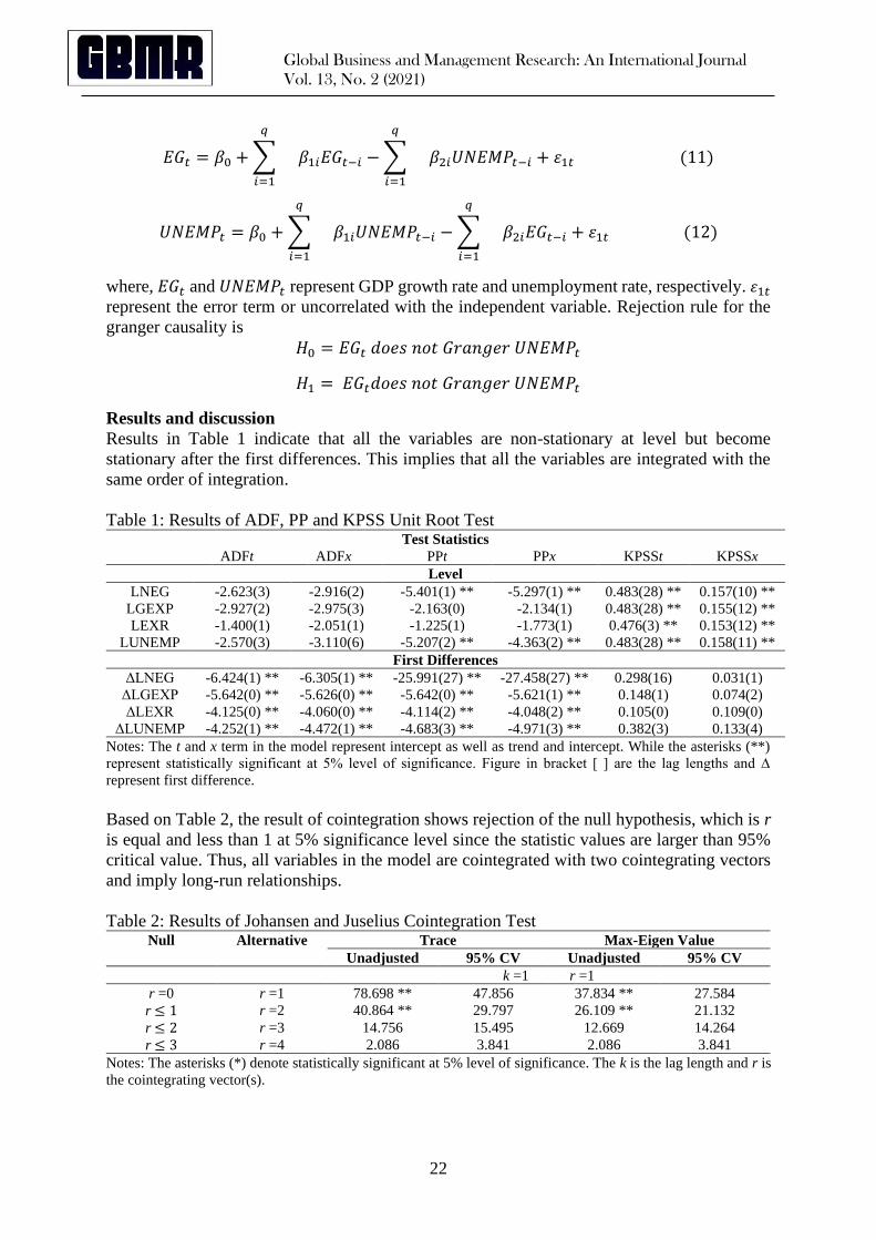
Results and discussion

Results in Table 1 indicate that all the variables are non-stationary at level but become

stationary after the first differences. This implies that all the variables are integrated with the

same order of integration.

Table 1: Results of ADF, PP and KPSS Unit Root Test Test Statistics

ADFt ADFx PPt PPx KPSSt KPSSx

Level

LNEG -2.623(3) -2.916(2) -5.401(1) ** -5.297(1) ** 0.483(28) ** 0.157(10) **

LGEXP -2.927(2) -2.975(3) -2.163(0) -2.134(1) 0.483(28) ** 0.155(12) **

LEXR -1.400(1) -2.051(1) -1.225(1) -1.773(1) 0.476(3) ** 0.153(12) **

LUNEMP -2.570(3) -3.110(6) -5.207(2) ** -4.363(2) ** 0.483(28) ** 0.158(11) **

First Differences

ΔLNEG -6.424(1) ** -6.305(1) ** -25.991(27) ** -27.458(27) ** 0.298(16) 0.031(1)

ΔLGEXP -5.642(0) ** -5.626(0) ** -5.642(0) ** -5.621(1) ** 0.148(1) 0.074(2)

ΔLEXR -4.125(0) ** -4.060(0) ** -4.114(2) ** -4.048(2) ** 0.105(0) 0.109(0)

ΔLUNEMP -4.252(1) ** -4.472(1) ** -4.683(3) ** -4.971(3) ** 0.382(3) 0.133(4)

Notes: The t and x term in the model represent intercept as well as trend and intercept. While the asterisks (**)

represent statistically significant at 5% level of significance. Figure in bracket [ ] are the lag lengths and ∆

represent first difference.

Based on Table 2, the result of cointegration shows rejection of the null hypothesis, which is r

is equal and less than 1 at 5% significance level since the statistic values are larger than 95%

critical value. Thus, all variables in the model are cointegrated with two cointegrating vectors

and imply long-run relationships.

Table 2: Results of Johansen and Juselius Cointegration Test Null Alternative Trace Max-Eigen Value

Unadjusted 95% CV Unadjusted 95% CV

k =1 r =1

r =0 r =1 78.698 ** 47.856 37.834 ** 27.584

r ≤ 1 r =2 40.864 ** 29.797 26.109 ** 21.132

r ≤ 2 r =3 14.756 15.495 12.669 14.264

r ≤ 3 r =4 2.086 3.841 2.086 3.841

Notes: The asterisks (*) denote statistically significant at 5% level of significance. The k is the lag length and r is

the cointegrating vector(s).


Vol. 13, No. 2 (2021)

23

The equation below shows there is an existence of long-run relationships between LNEG and

LGEXP as well as LNEG and LUNEMP. The relationship between LGDPGR and LGEXP

increases 1% in LGEXP will increase by 17.65% in LNEG. The positive impact of government

expenditure on growth is consistent with studies of Hong et al. (2016), Hasnul (2015) and Sinha

(1998). For the relationship between LNEG and LUNEMP, an increase 1% in LUNEMP will

increase 19.91% in LNEG. This result is supported by studies of Kogid et al. (2012) and

Minescu (2012). While LNEG has a negative relationship with LEXR, increasing 1% in LEXR

will decrease 18.15% in LNEG. This is consistent with the study by Mosikari (2013).

LNEG = -43.9373 + 17.6508*LGEXP - 18.1512*LEXR + 19.9146*LUNEMP

Table 3: Results of Normalized Equation Test LNEG C LGEXP LEXR LUNEMP

1.0000 -43.9373 17.6508

(-3.5441)

-18.1512

(4.8426)

19.9146

(-4.6379)

Notes: (**) denotes statistically significant at 5% level. Numbers in brackets are 𝑡-statistics

Table 4 shows the result of causality test with the ECT based on VECM. LNEG equation is the

only one in the system where the t-statistics of the ECT is statistically significant. The ECT

coefficient indicates the responsiveness of the short adjustment to the long-run equilibrium.

The adjustment is about 21.06 percent annually, 57 months or 4.75 years to respond to the long-

run equilibrium due to temporary shocks. Full adjustment (100%) = 12 months/21.06% × 100%

= 57 months

Table 4: Results of Vector Error Correction Model on Granger Causality Test Dependent Variables Δ LNEG ΔLGEXP ΔLEXR ΔLUNEMP ECT

χ² Statistics Coefficient 𝑡-ratio

Δ LNEG - 6.976

(0.031) **

2.070

(0.355)

2.575

(0.276)

-0.211 -2.209

ΔLGEXP 0.558

(0.757)

- 0.337

(0.845)

12.254

(0.002) **

0.009 1.761

ΔLEXR 1.179

(0.555)

3.082

(0.214)

- 8.578

(0.014) **

0.010 1.557

ΔLUNEMP 8.006

(0.018) **

1.169

(0.557)

2.003

(0.367)

- 0.028 7.026

Notes: Δ refers to first difference operator. Asterisks (**) indicate statistically significant at 5 percent level. Values

in parentheses indicate the probability value.

Diagram below shows the causality association between LNEG, LGEXP, LEXR and

LUNEMP. There is no bidirectional causality that runs among the variables. However, there is

a unidirectional causality that run from LNEG to LUNEMP, LUNEMP to LEXR and

LUNEMP to LGEXP in short-run. There is also a unidirectional causality from LGEXP to

LNEG which is consistent with Jiranyakul (2007) result. Thus, there is an indirect causality

that runs from LGEXP to LEXR through LNEG to LUNEMP, which is consistent with the

result of Minescu (2012).

In order to further examine the dynamic aspect of the relationship between government

expenditure, exchange rate and unemployment, this study employs Variance Decomposition

and Impulse Response. The purpose of the Variance Decomposition is to identify which

variable is the most exogenous in the system in the long term. Meanwhile, Impulse Response

aims to examine the decay period of the effect of short-run shock. Based on Table 5, LUNEMP

is the most interactive variable in the system where 97 percent of the error variance can be


Vol. 13, No. 2 (2021)

24

described by LNEG (36 percent), LGEXP (24 percent) and LEXR (37 percent) at the end of

50 years horizon. Furthermore, LUNEMP is the most endogenous variable and LNEG is the

most exogenous variable in the system.

Figure 6: Summary of Short-Run Causal Linkage

Table 5: Results of Variance Decomposition Percentage of Horizon Due to innovation in:

variations in (Years) ∆LNEG ∆LGEXP ∆LEXR ∆LUNEMP ΔCU

Years relative variance in: ∆LNEG

1 100.000 0.000 0.000 0.000 0.000

4 68.028 9.108 12.736 10.129 31.972

12 66.946 10.281 15.422 7.351 33.054

20 67.681 10.346 16.097 5.876 32.319

30 68.189 10.400 16.482 4.929 31.811

40 68.484 10.433 16.706 4.377 31.516

50 68.678 10.455 16.852 4.015 31.322

Years relative variance in: ∆LGEXP

1 33.248 66.752 0.000 0.000 33.248

4 28.645 63.948 1.410 5.997 36.052

12 21.077 64.840 5.268 8.814 35.160

20 18.887 64.964 6.404 9.745 35.036

30 17.473 65.035 7.146 10.345 34.965

40 16.673 65.078 7.564 10.685 34.922

50 16.158 65.106 7.833 10.904 34.894

Years relative variance in: ∆LEXR

1 51.101 1.041 47.858 0.000 52.142

4 44.519 3.943 50.132 1.406 49.868

12 47.741 7.385 44.387 0.487 55.613

20 48.565 7.417 43.686 0.332 56.314

30 48.991 7.465 43.295 0.249 56.705

40 49.209 7.488 43.096 0.207 56.904

50 49.341 7.502 42.976 0.182 57.024

Years relative variance in: ∆LUNEMP

1 5.235 10.425 0.049 84.291 15.709

4 26.849 6.388 50.569 16.194 83.806

12 34.496 20.331 40.965 4.209 95.791

20 35.449 22.718 38.437 3.396 96.604

30 35.866 23.735 37.388 3.010 96.990

40 36.063 24.216 36.891 2.830 97.170

50 36.177 24.496 36.602 2.725 97.275

Notes: The last column provides the percentage of forecast error variances of each variable explained collectively

by the other variables. The column in bold represent the impact of their own shock.


Vol. 13, No. 2 (2021)

25

The impulse response is generated to describe how the variable tends to react over the time due

to exogenous impulse. Generally, all variables become stable in long-run and start 20 years

interval. Based on the graph above, when the shock is variable LUNEMP, the variable LGEXP

is facing a big fluctuate at the beginning but later become stable after 20 years, the same cases

when the shock is LEXR to response to LGEXP. When the shock is LUNEMP, the variable

LENG decrease at the beginning until 10 years and increase again to 15 years, after that is

becomes stable starting 20 years.

Figure 7: The results of Impulse Response Function

Conclusion

The study aims to examine the impact of government expenditure, exchange rate, and

unemployment rate on Malaysia's economic growth. The outcome shows that government

expenditure has a positive association with Malaysia's economic growth in the long run. In

contrast, the exchange rate and unemployment rate have a significant negative and positive

relationship with Malaysia's economic growth. Besides, there is unidirectional causal

relationship among the variables that run from LGEXP to LNEG, LNEG to LUNEMP,

LUNEMP to LEXR and LUNEMP to LGEXP. Thus, there is an indirect causality that runs

from LGEXP to LEXR through LNEG to LUNEMP. Therefore, policymakers should focus on

fiscal policy and exchange rate policy. Government expenditure remains an essential tool in

stimulating the economic growth of Malaysia. In the meantime, ensuring manageable level of

exchange rate and unemployment also critical in providing stability and conducive business

environment.


Vol. 13, No. 2 (2021)

26

Acknowledgement

Financial support from Universiti Malaysia Sarawak (UNIMAS) is gratefully acknowledged.

References

Abas, A. (2017, November 17). Malaysia’s Q3 GDP Growth Rate Among the Highest in

Asia. New Straits Times, Retrieved from

https://www.nst.com.my/news/nation/2017/11/304391/malaysias-q3-gdp-growth rate-among-

highest-asia

Alhdiy, F. M., Johari, F., Nurazara, S., & Asma, A. R. (2015). Short- And Long-Term

Relationship Between Economic Growth and Unemployment in Egypt. Mediterranean

Journal of Social, 6(4), 454-462.

Awam, R. U., Azid, T., & Sher, F. (2011). Growth Implications of Government Expenditures

in Pakistan: An Empirical Analysis. Interdisciplinary Journal of Contemporary Research

in Business, 3(3), 451-472.

Bilson, J.F.0. (1978). Rational Expectations and the Exchange Rate. In Frenkel, J.A. and

Johnson, H.G. (eds.) The Economics of Exchange Rates: Selected Studies. Reading,

Mass: Addison-Wesley, 1978.

Dickey, D. A., & Fuller, W. A. (1981). Likelihood Ratio Statistics for Autoregressive Time

Series with a Unit Root. Econometrica, 49(4), 1057-1072.

Dornbusch, R. (1976). Capital Mobility, Flexible Exchange Rates and Macroeconomic

Equilibrium." In Claassen, E. and Salin, P. (eds.) Recent Issues in International Monetary

Economics. Amsterdam: North-Holland, l976a. Pg. 29-48.

Frenkel, J. A. (1976). A Monetary Approach to the Exchange Rate: Doctrinal Aspects and

Empirical Evidence. Scandinanvian Journal of Economics, 78(2), 200-224.

Granger, C. W. J., & Aug, N. (1969). Investigating Causal Relations by Econometric Models

and Cross-spectral Methods. Econometrica, 37(3), 424-438.

Hasnul, A. G. (2015). The Effects of Government Expenditure on Economic Growth: The Case

of Malaysa. Munich Personal RePEc Archive, No. 71254.

Hill, R. (2015, September 17). Malaysia: Political and financial instability shake confidence.

FocusEconomcs. Retrieved from https://www.focus-

economics.com/countries/malaysia/news/exchange-rate/political-and-financial-

instability-shake-confidence

Johansen, S., & Juselius, K. (1990). Maximum Likelihood Estimation and Inference on

Cointegration with Applications to Demand for Money. Oxford Bulletin of Economics

and Statistics, 52, 169-210.

Kogid, M., Asid, R., Lily, J., Mulok, D., & Loganathan, N. (2012). The Effect of Exchange

Rates On Economic Growth in Malaysia: Empirical Testing on Norminal versus Real.

The JUP Journal of Financial Economics, X(1), 7-17.

Lee, C. & Law, C. H. (2013). The Effects of Trade Openness on Malaysian Exchange Rate.

Munich Personal RePEc Archive, No. 45185.

Minescu, A. C. (2012). The Real Exchange Rate: A Factor in The Economic Growth? The

Case of Romania, Jonkoping International Business School.

Mosikari, T. J. (2013). The Effect of Unemployment Rate on Gross Domestic Product: Case

of South Africa. Mediterranean Journal of Social, Vol.4, No.6.

Phillips, P. C. B. & Perron, P. (1988). Testing for a Unit Root in Times Series Regression.

Biometrica, 75(2), 335-446. Rodrik, D. (2008). The Real Exchange Rate and Economic Growth: Brookings Papers on

Economic Activity.

https://www.nst.com.my/news/nation/2017/11/304391/malaysias-q3-gdp-growth%20rate-among-highest-asia

https://www.nst.com.my/news/nation/2017/11/304391/malaysias-q3-gdp-growth%20rate-among-highest-asia

https://www.focus-economics.com/countries/malaysia/news/exchange-rate/political-and-financial-instability-shake-confidence




Vol. 13, No. 2 (2021)

27

Sinha, D. (1998). Government Expenditure and Economic Growth in Malaysia. Journal of

Economic Development, 23(2), 71-80.

Wong, H. C., Khin, A. A., & Alexandar, T.G.M. (2016). Public Expenditure and Economic

Growth in Malaysia. International Conference on Accounting Studies (ICAS).

World Bank. (2020). Washington, DC: World Bank.

impact of government expenditure, exchange rate and

Documents