1

Impact of COVID-19 on Civil Aviation Stock Shares: Special

of Turkey

Su Lal Ayas1 Department of Astronautical Engineering, Istanbul Technical University

Yusuf Barış Metin2 Department of Astronautical Engineering, Istanbul Technical University

Prof. Dr. İbrahim Özkol3 Department of Aeronautical/Astronautical Engineering, Istanbul Technical University

I.Abstract

The Novel coronavirus disease (COVID-19) is an infectious disease caused by a virus and originated in Wuhan

city, Hubei Province in China. The virus has first detected at the end of December 2019 and spread all over the world

in a couple of months, becoming a global concern as it has started to kill thousands of people. Since then, almost all

countries have had to respond to it in different ways such as practicing severe hygienic measures, national and

international lockdowns, and even herd immunity. As a result, all the industries inevitably, so the economy all over

the world has been severely affected. Especially tourism, so the aviation industry is having the worst crisis of its

history. The COVID-19 is rattling the aviation stock market. This report examines the short-term effects of the 2019

novel coronavirus (COVID-19) pandemic on selected airline stocks. Firstly, the paper gives background information

about how COVID-19 is spreading all over the world, also impacting the aviation industry with evidence of a decline

in world air passenger traffic. Then, it examines how the aviation industry struggled with crises in history such as

9/11, SARS disease, and Iraq War so that it gives an idea of what can happen this time with COVID-19. Further, it

gives specific information cited from trading related news agencies such as a decline in stock shares of several airlines

from the USA and Turkey. After that, the main goal of the study is to model, then predict the volatility of stock indexes

in the Turkish civil aviation industry. Here the proper GARCH models are selected considering more accuracy in

results, then applied to the dataset of the daily closing prices of Turkish Airlines and Pegasus Airlines for a specific

time period. The results show the change in holistic volatility of Turkish Civil Aviation Industry due to COVID-19

and how the different responses from Turkish Airlines and Pegasus Airlines to COVID-19 have impacted their stock

shares. Finally, VaR estimation is obtained to forecast the worst possible losses in shares, which provides significant

information about the favorability of the business. At the end, the paper discusses that whether more positive attitude

and measures to COVID-19 help airlines to diminish the effects of the pandemic.

II.Introduction and Objectives

Since the declaration of the COVID-19 global

pandemic by the World Health Organization (WHO)

on March 11, 2020, many industries have been

experiencing the new normal acutely negative by

means of downsizing. Haydon & Kumar states that

the airline industry had been pioneering among the

most impacted industries by the pandemic among the

leisure facilities, restaurants, oil & gas drilling, and

the auto parts & equipment sector [1]. Apart from the

economic damages caused by the epidemic, the

1 ayas16@itu.edu.tr 2 metiny15@itu.edu.tr 3 ozkol@itu.edu.tr

Figure 1. World Passenger Traffic Evolution [2]

2

airline industry had already been in decline since 2019 due to the US-China trade war and the grounding problem of

the Boeing 737 Max.

In addition to the existing decline, as it can be seen in the Figure 1, the coronavirus pandemic had caused a 60%

decline in world total passengers in 2020 and a total revenue loss of 370 billion dollars according to the ICAO data

updated on 20 January 2020. However, the commercial air travel sector is extremely familiar with the natural, social,

and public health crises since the 20th century starting with the 1968 Hong Kong flu causing a death number estimated

up to 4 million globally. Stanley indicates that the Hong Kong flu is the world’s first globally spread epidemic through

the scientific achievement of flight. Nevertheless, the death rates of the first 2 years of Hong Kong flu weren’t standing

out compared to the average seasonal flu death rates consequently precaution in the industry hadn’t been properly

followed [3]. Following the 1968 pandemic, the 1973 oil embargo by the Organization of Arab Petroleum Exporting

Countries had forced the airlines to adapt to new

strategies to prevent revenue loss. Teyssier refers that

oil price had increased 400% and new strategies had

been declared by ICAO in terms of decreasing the

flight frequencies, prioritizing the commercial air

transport, and maximum coordination on fuel supply

to be satisfied in order to keep the necessary

operation of air services [4]. In addition to these

resolutions, carriers also stopped painting the planes

to reduce the weight and started flying at lower

speeds to economize on fuel consumption. The two

major crises which had characterized the economy of

the commercial airline industry and the world

economy through the modern-day were in the early

2000s: the September 11 terrorist attack and the

SARS outbreak. According to Cento, it took about 17

months for carriers to recover in terms of revenue

passenger kilometers (RPK) and 18 months in terms

of available seat kilometers (ASK) after the terrorist

attack. In this duration, carriers had reacted to the

crisis by decreasing capacity supply by reducing

frequencies and switching to smaller aircrafts or

canceling the routes [5]. Despite of the adjustments

and strategies afterward the attack, the volume of air

travel had a permanent decrease and airfares have

been permanently reduced to 10 percent [6]. Sehl

points out that apart from the COVID-19 outbreak,

the 9/11 terrorist attack had resulted in the steepest decline in air traffic. The travel demand had dropped to 30% in

the US immediately after the incident and it took about 6 years for the airline industry to fully recover. COVID-19

outbreak outperforms the 9/11 terrorist attack, causing more than 140 airlines to reduce their capacity down to 10%

or less [7]. The severe acute respiratory syndrome (SARS) epidemic on the other hand were the first major epidemic

harming the airline industry. Even though it was less impactful than the 9/11, the outbreak appeared 1.5 years after

the terrorist attack and challenged the economic recovery. During the SARS epidemic, a total of 8000 people had been

infected and 774 of them died according to WHO [8]. Although the death numbers were relatively few, the loss of

confidence and uncertainty led to a chain reaction in key sectors, thus, harsh economic damages. Cento indicates that

the demand reached its lowest point (-30%) 3 months after the global declaration in terms of RPK, even lower than

the 9/11 RPK values. ASK values decreased drastically in the second quarter of 2003 and carriers in almost every

continent had decreasing ASK index ranging from 18 percent to 8. The carriers reacted to the crisis by reducing

frequency, aircraft size, and routes, similar to the previous crisis. Additional to the adjustments, triangular services

were introduced to keep the Asian routes. SARS caused an annual decline for nearly 2 decades in the route of Asia –

pacific traffic. Comparing the SARS and 9/11 crises, it is seen that they resemble in terms of shock magnitude but

differs in terms of time duration. A demand reduction about 30-36% was reached by both crises but SARS epidemic

effects lasted for 6-7 months whereas the September 11 effects lasted for 17 months. In terms of carrier reaction, the

adjustments were similar but the reaction to SARS was quicker and limited [5]. One natural crisis that affected the

airlines were the 2010 eruptions of Iceland’s volcano, Eyjafjallajökull. In mid-April, the European airspace was forced

Figure 2. ASK index for traffic flows from Europe to

Asia [5]

Figure 3. ASK index for traffic flows from Europe to

North America [5]

3

to close over a period of 7 days due to the possible damages to the aircraft engines by the ash plume. It is stated that

this closure was the largest air traffic shut down since World War II. According to Bisignani, 100,000 flights were

cancelled and a revenue loss of $1.7 billion was reached during the shut-down. 19k flights per day were cancelled at

the peak duration of eruption and grounding was up to 30 percent. More than 10 million people were unable to travel

and the airlines also had to cover the expenses for hotel accommodation and other facilities for these passengers [9].

The eruption of Eyjafjallajökull showed the significance of the aviation sector and risk management during a crisis.

However, it is predicted that the survival of the industry is going to be different compared to the other shocking events

the industry had survived in the past, therefore this time, the world is facing a much more serious problem.

Although it is still unclear, COVID-19 has first identified in December 2019, Wuhan, China. It is declared as a

pandemic in March 2020 by WHO and as of today- 1 December 2020 approximately 63.2 million cases have been

confirmed with a total of 1.46 million deaths related to it according to BBC. The pandemic keeps peaking every week

in all major countries which destabilizes the world’s economy. WHO indicates that COVID-19 spreads between

people, mainly when an infected person is in close contact with another person. Coughing, sneezing, talking, and

laughing may help the virus to spread to the environment via respiratory droplets [10]. Therefore, since day 1 of the

pandemic, authorities have been strongly advising the public to maintain at least 1-meter distance between another

person, wear masks, care for good hygiene and reduce the close physical interaction with other people such as staying

home, avoiding crowds, and gatherings. Even though governments were unwilling to take a step to follow advises at

the beginning, they had to start putting restrictions on public once the pandemic has started raging out of control. By

13 March 2020, the cases in Europe outnumbered China that led WHO to announce Europe as the epicenter of the

COVID-19 [11]. EU countries have restricted free movement in the Schengen Area, many of them closed their borders

to foreign citizens, and quarantine and curfew orders have come into force. As of 30 April 2020, all countries in Asia

had reported at least one case except North Korea and Turkmenistan which are ruled by dictatorship. Although some

Asian countries such as Vietnam and South Korea handled better by responding fast, they still practice strong travel

restrictions as well as quarantines and other nationwide measures. On March 13, The President of the USA declared

a national emergency, however, the fact that President Trump downplayed the threat and refused the shut down the

country led them to reach the highest number of cases in the world. Although all states practice some restrictions now,

the USA is still open to other countries and has surpassed 13.9 million cases with more than 274 thousand deaths by

1 December 2020. According to The Washington Post, the virus has spread to South America on 26 February 2020

and the rapid increase of cases in Brazil caused the WHO to declare South America the epicenter of the pandemic

[12]. The virus has arrived in Egypt, so Africa on 14 February. According to The Guardian, by 26 May, more than

half of African countries were facing community transmission due to lack of test kits, health infrastructure, and being

unable to shut down the economy [13]. Oceania has reported the first case on 25 January 2020 and the virus has spread

widely in Australia and New Zealand since then [10]. However, both countries handled better with early serious

precautions and closed their international borders. Besides the fear and the individual responses, national and

international responses by governments have made a huge impact on broad aspects of our daily life including

economy, culture, ecology, politics, and mental health. Coronavirus travel restrictions across the globe, decrease in

purchasing power due to hundreds of millions losing their job or facing fall in their income have caused tourism to

Figure 4. RPKs and ASKs development

for the traffic flows from Europe to North

America [5]

Figure 5. RPKs and ASKs development for

the traffic flows from Europe to Asia [5]

4

become one of the worst affected sectors, so does the aviation industry. Significant slumps in demand among travelers

and travel restrictions have resulted in flight cancellations or empty flights which leads the aviation industry to the

biggest crisis of history. The main problem here is that it is still unclear how long the pandemic will last. Pfizer and

BioNTech announced their mRNA-based vaccine candidate with strong evidence of efficiency against COVID-19. A

week later, on 16 November 2020, Moderna followed them claiming their vaccine has a success rate of 94.5%. Only

a few countries have started mass vaccination as of the 28th of December. However, WHO estimates vaccine will be

ready for widespread distribution around mids of 2021 [10].

Considering all the restrictions and uncertainty of the timeline of the pandemic, there is no surprise that the airline

industry might be on the verge of collapse. Airline stock shares are slumped so badly that it is record breaking. Forbes

states that ‘For the full year, JetBlue was down 22%. Alaska was down 23%. Delta was down 31%. Spirit was down

39%. American Airlines was down 45%. United was down 51%.’ [14]. The situation is not different at all for the

Turkish Civil Aviation Industry. Atlas Global which had been facing financial problems since 2018, had already filed

bankruptcy in February [15]. According to Reuters, Turkish Airlines’ passenger number has decreased 65.9% in

August compared to a year before and the company declared a 2.23 billion liras (287 million USD) loss since the

lockdowns at home and abroad were started in the second quarter. As it can be seen in the Figure 2, Turkish Airline

shares slumped approximately 50% in a month at the beginning of the pandemic. As of the 23rd of January, the stock

price is 12.89, trying to cover the loss. The company has been trying to reduce the cash burn and build liquidity by

state aids and various strategies such as cutting employee’s wages by 30-50%, rearranging flight schedules, and

offering more deals for future flights [16].

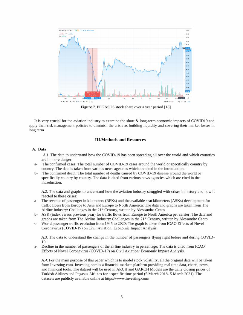
It is not different at all for another major Turkish Civil Aviation company, Pegasus. Figure 7 shows that Pegasus

stocks slumped almost 68% within a month after travel restrictions were applied. We can see that there is a spike

around May when the first big wave was fading and many countries were eager to open for tourism. However, right

after summer, a second big wave hit almost everywhere resulted in more severe travel restrictions, so that stock shares

slumped again. As of the 26th of January, as positive news about vaccination and restrictions being effective,

PEGASUS stock share has managed to climb up to 72.3, a peak since February.

Figure 6. TURK HAVA YOLLARI stock share over a year period [17]

5

It is very crucial for the aviation industry to examine the short & long-term economic impacts of COVID19 and

apply their risk management policies to diminish the crisis as building liquidity and covering their market losses in

long term.

III.Methods and Resources

A. Data

A.1. The data to understand how the COVID-19 has been spreading all over the world and which countries

are in more danger:

a- The confirmed cases: The total number of COVID-19 cases around the world or specifically country by

country. The data is taken from various news agencies which are cited in the introduction.

b- The confirmed death: The total number of deaths caused by COVID-19 disease around the world or

specifically country by country. The data is cited from various news agencies which are cited in the

introduction.

A.2. The data and graphs to understand how the aviation industry struggled with crises in history and how it

reacted to these crises:

a- The revenue of passenger in kilometers (RPKs) and the available seat kilometers (ASKs) development for

traffic flows from Europe to Asia and Europe to North America: The data and graphs are taken from The

Airline Industry: Challenges in the 21st Century, written by Alessandro Cento

b- ASK (index versus previous year) for traffic flows from Europe to North America per carrier: The data and

graphs are taken from The Airline Industry: Challenges in the 21st Century, written by Alessandro Cento

c- World passenger traffic evolution from 1945 to 2020: The graph is taken from ICAO Effects of Novel

Coronavirus (COVID‐19) on Civil Aviation: Economic Impact Analysis.

A.3. The data to understand the change in the number of passengers flying right before and during COVID-

19:

a- Decline in the number of passengers of the airline industry in percentage: The data is cited from ICAO

Effects of Novel Coronavirus (COVID‐19) on Civil Aviation: Economic Impact Analysis.

A.4. For the main purpose of this paper which is to model stock volatility, all the original data will be taken

from Investing.com. Investing.com is a financial markets platform providing real time data, charts, news,

and financial tools. The dataset will be used in ARCH and GARCH Models are the daily closing prices of

Turkish Airlines and Pegasus Airlines for a specific time period (5 March 2018- 5 March 2021). The

datasets are publicly available online at https://www.investing.com/

Figure 7. PEGASUS stock share over a year period [18]

6

B. Methods

Both ARCH and GARCH models will be used to model and estimate the volatility of stock indexes in the Turkish

Civil Aviation Industry. The autoregressive conditional heteroscedasticity (ARCH) model will describe a changing,

possibly volatile variance in stock indexes of selected Turkish aviation companies. In other words, it will help us to

estimate the risk and forecast future volatility. Generalized Autoregressive Conditional Heteroskedasticity (GARCH)

will be also used to predict the volatility of returns on stocks and assess the risk. The process will be conducted on

Matlab and the dataset is the daily closing prices of Turkish Airlines and Pegasus Airlines for a specific time period.

B.1. ARCH Model [19][20][21]

The autoregressive conditionally heteroscedasticity (ARCH), introduced by Engle (1982) is a statistical model for

the variance of a time series. This model focuses on modeling the volatility of the variance of the series. It is used in

the context of finance problems that consist of financial asset investments or stock change in a specific time interval.

It could be used to model any series that periods of variance change such as volatility in stock prices, oil prices, GDP,

poverty rates, and inflation rates. As applying the ARCH model, the residuals must be squared, the correlogram must

be examined and the mean of the residuals must be zero.

ARCH(p):

A time-series {ϵ(t)} is given at each instance by

ϵ(t) = w(t) × σ(t)

Where w(t) is the white noise with zero mean and unit variance.

var(x(t)) = σ²(t) = ⍺0 + ⍺1 × σ2(𝑡−1)

Where ⍺0, ⍺1 are parameters of the model and to make conditional variance positive; ⍺0 > 0, ⍺1 ≥ 0.

σ²(t-1) is lagged square error.

Here ϵ(t) is an autoregressive conditional heteroskedastic model of order unity, denoted by ARCH (1):

ϵ(t) = w(t) × σ(t) = w(t) × √(⍺0 + ⍺1 × ϵ²(t−1))

By same process, ARCH (2):

ϵ(t) = w(t) × σ(t) = w(t) × √(⍺0 + ⍺1 × ϵ²(t−1) + ⍺2 × ϵ2(t−2)))

So basically, the general formula is:

ϵ(t) = w(t) × σ(t) = w(t) × √⍺0 + ⍺p × ∑ ϵ²𝑡−1

𝑝

𝑖=1

Where p is the number of lag squared residual errors to include in the ARCH model and i= (1,2,….,p) is the number

of logged periods of the square error.

How do we interpret the ARCH model:

1- If the error is high during the given time period of (t-1), the value of error at the period (t) is likely to be

higher.

2- If the error is low during the given time period of (t-1), the value of error at the period (t) is likely to be

lower.

3- ⍺1 should be equal to or greater than zero for the positive variance

4- ⍺1 should be smaller than 1 for stability conditions, if not, ϵ(t) will continue to increase over time.

7

To integrate ARCH model in stock volatility, the below equation is derived from variance formula:

var(ϵ(t)) = ⍺0 + ⍺1 × var(𝜖(𝑡−1))

It can be seen that the variance of the series is a linear combination of the variance of the prior element of the

series. In other terms, supposing S(i) is the value of a variable on a day (i), the standard deviation of ln(𝑆(𝑖)

𝑆(𝑖−1))

gives us the volatility per day.

B.2. GARCH Model [19] [22]

Generalized AutoRegressive Conditional Heteroskedasticity (GARCH), introduced by Bollerslev (1986, Journal

of Econometrics), is a statistical model that analyses time-series data where the variance error is believed to be serially

autocorrelated. It is an extension of the ARCH model which assumes that the variance of the error term follows an

autoregressive moving average process. This extension helps us to model the conditional change in variance over time

and allows the model to change in the time dependent variance.

GARCH(p,g):

As a difference from ARCH, here we will consider a single moving average lag besides a single autoregressive

lag. A time-series {ϵ(t)} is given as:

ϵ(t) = w(t) × σ(t)

Where w(t) is the white noise with zero mean and unit variance and ⍺0, ⍺1and β1 are parameters of the model. To

make conditional variance positive; ⍺0 > 0, ⍺1 ≥ 0, β≥0

Here we add moving average term σ²(t) to ARCH formula

ϵ(t) = w(t) × σ(t) = w(t) × √(⍺0 + ⍺1 × ϵ2(t−1) + β1 × σ²(t−1) )

By same process, the general formula of GARCH(p,q):

ϵ(t) = w(t) × σ(t)

σ2 = ⍺0 + (∑(⍺i

𝑞

𝑖=1

× ϵ2(t−i))) + (∑(βj

𝑝

𝑗=1

× σ²(t−j)))

How do we interpret the GARCH model:

1- The large value of β1 causes σ(t) to be highly correlated with σ²(t−1) and gives the conditional standard

deviation process a relatively long-term persistence, at least compared to its behavior under an ARCH

model.

2- If p is 0, the model reduces to the ARCH(q) process.

3- If both p and q are 0, ϵ(t) is simply white noise.

B.3. Value at Risk Forecast

Value at Risk is commonly used risk measuring method for financial markets. It refers to the maximum loss over

a targeted horizon for a given level of confidence. Namely, it estimates how much an investor might lose given

normal market conditions in a period of time. For instance, with a given confidence level such as 95%, it can be said

that the worst daily loss will not exceed VaR estimation.

IV.Analysis of The Resources for this Project To understand the background and purpose of the study, firstly we need to understand what COVID-19 is and how

it spreads. At this point, our main source is the World Health Organization (WHO) which is a specialized agency of

the United Nations and responsible for international public health. It is useful to build a relation how pandemic goes

and impacts the airline industry at the specific time that is examined. The International Civil Aviation Organization

(ICAO) reports are where the data of changes in air traffic for both around the world and specific countries are taken.

8

The main aim is to predict the future stock volatility of airline companies to help them diminish the financial

impact of COVID-19. Besides the stock model that is applied, how the commercial airline industry was affected by

major crises throughout its history should be considered. At this point, The Airline Industry: Challenges in 21st

Century written by Alessandro Cento is examined. In Chapter 3, Cento examines Short- and Long- Term Reactions

to Exogenous Demand Shifts. Here, he explains the terms such as the available seat kilometers (ASK) and the revenue

passenger kilometers (RPK), and what they mean for financial strategy of an airline. He collects the data of ASK and

RPK from Europe to North America; or Europe to Asia for a period of 43 months; from January 2000 to July 2003.

As he processes the data to graph, we see that how The September 11 Terrorist Attack, Iraq War, and SARS disease

impacted the civil aviation industry. To understand how ASK and RPK reacted to these crises will help us predict how

COVID-19 can impact the demand and supply for air traffic which is crucial for airline stock shares.

The other source will be articles that examine the use of ARCH&GARCH methods together on volatility problems.

The most significant part of the study to model volatility properly, so we can interpret the results truly. The related

articles guide us to implement the model properly on Matlab for our specific case. Volatility Modelling using Arch

and Garch Models (A Case Study of the Nigerian Stock Exchange) written by Kingsley Arum; Modelling Volatility

in stock prices using ARCH/GARCH technique written by K.Khan and U.M.Abdullah; and Using the GARCH model

to analyze and predict the different stock markets written by Wei Jiang will be examined for this purpose.

The main resources of the study are obtained from investing related agency, Investing.com. It provides the

historical data of daily closing stock prices of Turkish Airlines and Pegasus throughout the pandemic period. This

dataset is used to model ARCH&GARCH and estimate VaR to predict the volatility of future stock prices.

V.Modeling Process and Empirical Results

A. Logarithmic Returns of Stock Shares

One of the three methods to calculate return in statistics is log return. Specifically, for comparability of the time

series data of a long run activity such as markets, the log returns are used, since it is compounded continuously instead

of across sub periods. It is calculated by taking the natural logarithm of the ratio of two consecutive prices. By defining

a return rate 𝑟𝑖 at time 𝑖, where the daily price at time 𝑖 is 𝑝𝑖:

𝑟𝑖 = ln (𝑝𝑖

𝑝𝑖−1

)

Figure 8. Distribution of Log Returns of THYAO stock share over 3 years period (5 March 2018- 5 March 2021)

9

The distribution of log returns of THYAO and PEGASUS stock shares over 3 years period (5 March 2018- 5

March 2021) are represented in Figure 8 and Figure 9 respectively. It can be seen that the volatility changes on both

figures have a tendency to cluster financial returns over the time period which proves their long memory behavior.

Long memory indicates persistency in volatility. In other words, it means that financial markets do not forget large

volatility shocks: Large changes in volatility are followed by large changes, and small changes are followed by small

changes.

Figure 10 and Figure 11 illustrate the THYAO and PEGASUS QQ plots of the standardized residuals, respectively.

It can be seen that normality is rejected for the standardized residuals because of the excess kurtosis.

B. Suitability of Applying ARCH and GARCH

B.1. Descriptive Statistics and Jarque-Bera Test

Applicability of ARCH and GARCH models depends on if the shock that impacts volatility has asymmetric

distribution. To understand how the returns are distributed, statistical indicators such as mean, median, standard

deviation, skewness, kurtosis, and maximum and minimum values should be calculated; and the Jarque-Bera test

should be applied.

Figure 9. Distribution of Log Returns of PEGASUS stock share over 3 years period (5 March 2018- 5 March 2021)

Figure 10. THYAO Residual QQ Plot Figure 11. PEGASUS Residual QQ Plot

10

Table 1 shows daily observations’ descriptive statistics and Jarque-Bera test results for THYAO. The mean and

median of data are -0.00031248 and 0 respectively, with a standard deviation of 0.0263. The maximum value is 0.0957

and the minimum is -0.1619. The gap between minimum and maximum values proves the high variability of prince

changes. The skewness is a measure of the symmetry in distribution. In other terms, it basically measures the relative

size of two tails. Normally distributed series, meaning symmetrical series have a skewness of 0. THYAO returns have

a skewness of -0.221, so it is negatively(left) skewed, meaning the distribution has a left tail from normality. Another

parameter to understand the normality of distribution is the kurtosis value. Dr. Wheeler indicates that “The kurtosis

parameter is a measure of the combined weight of the tails relative to the rest of the distribution.”. In other terms, it

measures the tail heaviness of the distribution. The kurtosis decreases as the tails become lighter and increases as the

tails become heavier. The standard normal distribution has a kurtosis of 3. THYAO returns have a kurtosis of 6.1236

and it is called leptokurtic since it has excess positive kurtosis, where the kurtosis value is greater than 3. In other

terms, the tails are fatter than the normal distribution. In financial markets, leptokurtic returns indicate that risks are

coming from unusual events and the volatility can experience broader fluctuations that could result in greater potential

for very high or low returns. Finally, the Jarque-Bera test which is a type of Lagrange multiplier test is applied to

check the normality of distribution. More specifically, the test checks whether the skewness and kurtosis of the sample

data match a normal distribution. The test is run in Matlab Simulink and the result is 1, meaning the rejection of the

null hypothesis at the 5% significance level. Since the null hypothesis for the test is that the sample data is normally

distributed; the rejection means THYAO returns are not normally distributed.

Statistical Indicators Value Statistical Indicators Value

Mean -0.00031248 Kurtosis 6.1236

Median 0 Maximum 0.0957

Standard Deviation 0.0263 Minimum -0.1619

Skewness -0.221 Jarque-Bera 1

Table 2 shows daily observations’ descriptive statistics and Jarque-Bera test results for PEGASUS. The mean,

median, and the standard deviation of the data converge to 0. The maximum and minimum values are 0.1343 and -

0.1695 respectively. The gap between minimum and maximum values indicates that the high variability of prince

changes in PEGASUS data. The skewness is -0.1695, so the distribution is negatively(left) skewed, indicating the

distribution has a left tail from normality. Moreover, PEGASUS returns have a kurtosis of 5.1811, indicating

leptokurtic distribution where the results are more peaked than a normal distribution. Finally, the Jarque-Bera test is

applied. The test is run in Matlab Simulink and the result is 1. As it was explained previously, the result of 1 indicates

the rejection of the null hypothesis at the 5% significance level. In other terms, the PEGASUS data does not come

from a normal distribution.

As a result, it can be seen that the log returns of both PEGASUS and THYAO data are not normally distributed.

Also, the null hypothesis at the 5% significance level is rejected for both. All of the applied statistical analysis proves

the suitability of applying ARCH and GARCH models to estimate the volatility of shares of THYAO and PEGASUS.

Statistical Indicators Value Statistical Indicators Value

Mean 0* Kurtosis 5.1811

Median 0* Maximum 0.1343

Standard Deviation 0* Minimum -0.1695

Skewness -0.1159 Jarque-Bera 1

Table 1. Descriptive Statistics over 3 years of daily data of THYAO returns

Table 2. Descriptive Statistics over 3 years of daily data of PEGASUS returns

Note: * indicates data converges to 0

11

B.2. Time Series Characteristics and Unit Root Tests

An unexpected change in the variable or in the error term in a distinctive time period is defined as a shock. In

stationary time series, the effect of a shock diminishes in the progress of time. Meanwhile in time series, the effect of

a shock is permanent. Time series are stationary if they do not have trend or seasonal effects, meaning that, stationary

time series data do not depend on time. Many economic and financial time series data display nonstationarity or trend

characteristics. It is significant to properly determine the form of the trend characteristics of the data for an econometric

task in order to make forecasts for future behaviors. Posterior to determining the characteristics, usually trend removal

is necessary to stationarize the data because most statistical forecasting methods are based on the assumption that the

time series data is stationary. Unit root tests are used to determine whether the time series is stationary or nonstationary.

A unit root test tests whether a time series data is nonstationary by checking the possession of a unit root. The unit

root is defined as an aspect of a random process that may affect the statistical inference for the time series models.

The time series display an unpredictable and systematic pattern in the existence of a unit root.

Figure 12. An example of a potential unit root. Green line shows a path of recovery in the presence of a unit root.

Blue line shows the path of recovery in the absence of a unit root and the series is trend-stationary. Green line is

permanently below the trend even after the recovery.

It is important to specify the null hypotheses and the alternative hypotheses properly in order to identify the trend

characteristics of the data while testing for unit roots. The type of the test regression will be determined based on the

trend characteristics of the data under the alternative hypotheses. Generally, the null hypothesis represents the

existence of a unit root while the alternative hypothesis represents stationary or trend-stationary. There are many unit

root tests, particularly due to low statistical power. However, the augmented version of the Dickey-Fuller Test fits the

complex models with large data. The Dickey-Fuller test which is based on linear regression is enhanced into The

Augmented Dickey-Fuller Test due to serial correlation issues. ADF Test is more compatible with the stock share data

of Turkish Airlines and Pegasus for the mathematical model.

B.2.1. ADF Test

Said and Dickey (1984) enhanced the autoregressive unit root test into the Augmented Dickey-Fuller (ADF) test

to satisfy the general ARMA(p, q) models with unknown orders. With the assumption of the data satisfying the ARMA

format, the null hypothesis is tested that a time series yt is I(1) against the alternative that is I(0) in the ADF test. Based

on estimating the test regression [23]

𝑦𝑡 = 𝛽′ Dt + ∅𝑦𝑡−1 + ∑ 𝜑𝑗∆𝑦𝑡−𝑗𝑝𝑗=1 + 𝜀𝑡

where Dt is a vector of deterministic terms (constant, trend, etc.). The p lagged difference terms, ∆yt-j, are used to

approximate the ARMA structure of the errors, and the value of p is set so that the error εt is serially uncorrelated. The

error term is also assumed to be homoscedastic. The specification of the deterministic terms depends on the assumed

behavior of yt under the alternative hypothesis of trend stationarity as described in the previous section. Under the null

hypothesis, yt is I(1) which implies that ∅ = 1. The ADF t-statistic and normalized bias statistic are based on the least

squares estimates of 𝑦𝑡 and are given by

𝐴𝐷𝐹𝑡 = 𝑡∅=1 = ∅̂ − 1

𝑆𝐸(∅)

12

𝐴𝐷𝐹𝑛 = 𝑇(∅̂ − 1)

1 − �̂�1 − ⋯ − �̂�𝑝

An alternative formulation of the ADF test regression:

∆𝑦𝑡 = 𝛽′𝐷𝑡 + 𝜋𝑦𝑡−1 + ∑ 𝜑𝑗∆𝑦𝑡−𝑗 + 𝜀𝑡𝑝𝑗=1

where π = φ−1. Under the null hypothesis, ∆yt is I(0) which means that π = 0. The ADF t-statistic is then the usual t-

statistic for testing π = 0 and the ADF normalized bias statistic is 𝑇�̂� = (1 − �̂�1 − ⋯ − �̂�𝑝). The test regression is

often used in practice because the ADF t-statistic is the usual t-statistic reported for testing the significance of the

coefficient yt-1.

Briefly, low p values after running the test on MATLAB point out to stationarity. When the test statistics number gets

more negative, the p value converges to a smaller number and the test is more likely to reject the null hypothesis. [24]

B2.2. Ljung-Box Test

Ljung and Box (1978) developed a statistical test to test the overall randomness of a set of data. The test is

commonly used in ARMA modelling and is applied to the residuals of the model. The test is defined as:

𝑄 = 𝑛(𝑛 + 2) ∑�̂�𝑘

2

𝑛−𝑘

ℎ𝑘=1

where n is the sample size, h is the number of lags being tested, and �̂�𝑘 is the sample autocorrelation at lag k. The null

hypothesis is rejected when

𝑄 > 𝑋1−𝛼,ℎ2

where 𝑋1−𝛼,ℎ2 is the value on the chi-squared distribution for significance level of α and h degree of freedom.

A test result of p value < 0.5 indicates the rejection of null hypothesis assuming a 5% chance of mistake.

B.2.3. ARCH LM Test

Engle’s (1982) ARCH LM test is a Lagrange Multiplier test to identify autoregressive conditional

heteroscedasticity. It checks for the compatibility of the fitted linear regression model for the squared residuals. The

null hypothesis states that the residuals are homoscedastic, meaning that formed by a sequence of white noise. A p

value approaching to 0 is a strong evidence to reject the null hypothesis. The null hypothesis implies the nonexistence

of ARCH effect. GARCH model cannot be applied where there is no ARCH effect.

Test Statistics p-values

ADF Test -28.5706 1x10^(-3)

Box-Ljung Test (residuals) 29.7591 9.3789x10^(-4) df 10

ARCH LM Test 70.9502 2.7777x10^(-6) df 5

Table 3 and Table 4 represent the results of The Augmented Dickey-Fuller Test, Box-Ljung Test, and ARCH-LM

Test for THYAO and PEGASUS data, respectively. The results shown in the tables indicate that the p values of the

Test Statistics p-values

ADF Test -3.6897 1.00E-03

Box-Ljung Test (residuals) 43.73 3.68E-06 df 10

ARCH LM Test 184.4094 0 df 5

Table 3. Augmented Dickey-Fuller Test, Box-Ljung Test, and ARCH-LM Test for THYAO stock share over 3

years of period

Note: ** and *** represent the significance at the 5% and 1% levels, respectively.

Table 4. Augmented Dickey-Fuller Test, Box-Ljung Test, and ARCH-LM Test for PEGASUS stock share over

3 years of period

Note: ** and *** represent the significance at the 5% and 1% levels, respectively.

13

ADF test is small enough to reject the null hypothesis and the returns can be considered stationary. This approves the

non-existence of autocorrelation. Box-Ljung test gives p values smaller than 0.05 for both returns, satisfying the

rejection of the null hypothesis. Finally, for the ARCH LM test, p value is small enough to be considered as 0 for

THYAO, while it is already 0 for PEGASUS returns. This implies both the rejection of the null hypothesis and that

the ARCH effect can be observed in the log returns. Since the ARCH effect is present, the GARCH model can be

applied to the data set.

C. Selection of GARCH Model

Basically, descriptive statistics, Jarque-Bera test, and unit root tests have proved that there is an ARCH effect in

the return of both PEGASUS and THYAO data, therefore the GARCH model can be applied. At this phase, the order

of a GARCH model such as GARCH(1,1), GARCH(1,2), GARCH(2,1), GARCH(2,2) should be determined. Since

the goal of the project is to forecast volatility, a model that could deliver the most accurate forecasts should be selected.

To select the most accurate model, first, we should check the model’s goodness of fit to data by using Akaike

Information Criterion (AIC), Bayesian Information Criterion (BIC), then we should compare p values that are results

of Box-Ljung and ARCH LM Tests which are applied to four of the GARCH model options. The model with the

lowest AIC, BIC, and p values should be preferred.

Table 5 represents the estimation results of GARCH models for THYAO data. Akaike’s Information Criterion

(AIC) is a method to evaluate how well a model fits the data. It estimates the amount of information lost by a model,

so the quality of a set of statistical models can be compared to each other. The smallest AIC value indicates the best

model. However, AIC values of all the GARCH model options for THYAO data set are the same (-3.48). Bayesian

Information Criterion (BIC) is an alternative approach to select the model. The model with lowest BIC value should

be preferred, yet all the GARCH models have very close BIC values to each other. Therefore, we continue with

applying the Box-Ljung and ARCH LM Tests with lag values of 10, 15 and 20 to GARCH model options. For the

Box-Ljung Test, as it is explained before, a p value describes how possible the data would have occurred by chance;

a test result of p value < 0.05 indicates the rejection of null hypothesis assuming a 5% chance of mistake. The smaller

the p value, the stronger evidence to reject the null hypothesis. For the ARCH LM Test, as it is mentioned before, a p

value approaching to 0 is a strong evidence to reject the null hypothesis. Consequently, the GARCH (1,2) is selected

for the price returns of THYAO.

GARCH(1,1) GARCH(1,2) GARCH(2,1) GARCH(2,2)

Akaike Information

Criterion (AIC)

-3.48E+03 -3.48E+03 -3.48E+03 -3.48E+03

Bayesian Information

Criterion (BIC)

-3.47E+03 -3.46E+03 -3.46E+03 -3.46E+03

Box-Ljung Test (r2,

lag=10), p value

0.3234 0.3173 0.3235 0.3178

Box-Ljung Test (r2,

lag=15), p value

0.0961 0.09 0.0961 0.0953

Box-Ljung Test (r2,

lag=20), p value

0.0342 0.031 0.0342 0.0336

Box-Ljung Test (r2,

lag=25), p value

0.0089 0.0081 0.0089 0.0087

ARCH LM Test (r,

lag=10), p value

0.8138 0.8052 0.8138 0.819

ARCH LM Test (r,

lag=15), p value

0.9062 0.885 0.9062 0.9107

ARCH LM Test (r,

lag=20), p value

0.9135 0.9032 0.9135 0.9169

ARCH LM Test (r,

lag=25), p value

0.9513 0.9426 0.9513 0.9537

Table 5. Estimation Results of GARCH models for THYAO data

Note: r represents residuals

14

Table 6 represents the estimation results of GARCH models for PEGASUS data. Considering previously

mentioned indicators, we see that AIC and BIC values are too close to make a difference between models. Therefore,

we continue with checking the results (p values) of Box-Ljung and ARCH LM Tests. It can be seen that GARCH(2,2)

model is appropriate, since p values obtained from Box-Ljung Test are lower than others’, as p values from ARCH

LM Test are too close to others’ to make a significant difference. Hence, we select GARCH(2,2) for PEGASUS data.

D. GARCH Models

Figure 13 and Figure 14 represent GARCH models for THYAO and PEGASUS returns, respectively.

GARCH(1,1) GARCH(1,2) GARCH(2,1) GARCH(2,2)

Akaike Information

Criterion (AIC)

3.17E+03 -3.17E+03 -3.17E+03 -3.17E+03

Bayesian Information

Criterion (BIC)

3.16E+03 -3.15E+03 -3.15E+03 -3.15E+03

Box-Ljung Test (r2,

lag=10)

0.0756 0.0762 0.0756 0.0734

Box-Ljung Test (r2,

lag=15)

0.0071 0.0071 0.0071 0.0067

Box-Ljung Test (r2,

lag=20)

9.12E-04 9.21E-04 9.12E-04 8.49E-04

Box-Ljung Test (r2,

lag=25)

3.15E-04 3.20E-04 3.15E-04 2.87E-04

ARCH LM Test (r,

lag=10)

0.6772 0.676 0.6772 0.6811

ARCH LM Test (r,

lag=15)

0.7083 0.709 0.7083 0.7092

ARCH LM Test (r,

lag=20)

0.8023 0.8014 0.8023 0.8046

ARCH LM Test (r,

lag=25)

0.9249 0.9246 0.9249 0.9254

Table 6. Estimation Results of GARCH models for PEGASUS data

Note: r represents residuals

Figure 13. GARCH (1,2) model of THYAO

returns

Figure 14. GARCH (2,2) model of PEGASUS

returns

15

E. Persistence of selected GARCH models

Since the parameters of selected GARCH models are determined, the persistence should be checked to reject the

null hypothesis for the crosscheck of selected models. The persistence of a GARCH model refers to the decay speed

of large volatilities caused by shocks. In other terms, if the model is persistent, volatility from previous periods can be

used to estimate current volatility. The persistence is measured by summing all the parameter coefficients of a GARCH

model. The sum should be less than 1, otherwise the predictions of volatility tend to be explosive. [25] Yet, the sum

also should be close to 1, so that model is more persistent.

Parameters Value Standard Error t Statistics P-value

ω 1.18E-04 3.22E-05 3.674 2.39E-04

α 0.6498 0.0785 8.2804 1.23E-16

β 1 0.1523 0.0453 3.3624 7.73E-04

β 2 0.033 0.0453 0.7283 4.66E-01

Table 7 represents the parameters of GARCH(1,2) for THYAO data. By summing the coefficients:

𝛼 + 𝛽1 + 𝛽2 = 0.8254

Since the sum is less than 1, it can be said the null hypothesis is rejected; GARCH(1,2) is likely to fit the data well.

Parameters Value Standard Error t Statistics P-value

ω 2.49E-04 3.12E-04 0.7989 4.24E-01

α1 0.232 1.603 0.1447 8.85E-01

α 2 0.2249 0.9396 0.2394 8.11E-01

β 1 0.2533 0.0556 4.5599 5.12E-06

β 2 0.0717 0.4038 0.1775 8.59E-01

Table 8 represents the parameters of GARCH(2,2) for PEGASUS data. By summing the coefficients:

𝛼1 + 𝛼2 + 𝛽1 + 𝛽2 = 0.7819

which is less than 1. Therefore the GARCH(2,2) is persistent and the null hypothesis is rejected.

VI. VaR Results of Selected GARCH models Finally, VaR graph is built for the return of the stock prices by using the GARCH model. Since conditional

variances(h) of the return series is obtained, VaR formula which is related with h and confidence level (α) is used.

The VaR estimation to understand maximal monetary amount that can be lost with at 95% confidence level is

calculated as: [26]

𝑉𝑎𝑅α = −𝑍α × √ℎ𝑡

Where 𝑍α is the value of normal distribution for the level of probability (α = 0.95), and obtained as 1.65.

𝑉𝑎𝑅95% = −1.65 × √ℎ𝑡

Obtaining VaR graphs for both THYAO and PEGASUS returns:

Table 7. Estimation results of GARCH(1,2) for THYAO returns

Table 8. Estimation results of GARCH(2,2) for PEGASUS returns

16

It is observed in Figure 15 that VaR value has a consistency until the COVID-19 begins to affect the aviation

industry in February 2020. At the beginning of COVID-19, the highest value of VaR is observed, which indicates high

uncertainty and risk in stock prices of THYAO. Namely, an investor should expect a high risk and potential maximum

loss at the time when VaR value is peaked. It explains that the restrictions put due to COVID-19 has resulted in serious

volatility fluctuations where the investors were exposed to high risk, so the stock shares soared. However, we can also

see that as the pandemic is brought under control, VaR value jumps back to its usual range which shows the market is

less volatile and the risk has been lowered down

Figure 16 illustrates the VaR value and log returns of PEGASUS stock shares. It can be seen in February 2020,

COVID-19 causes the highest possibility of maximum monetary loss which makes the market riskier for business

activities. Then the VaR fluctuation range tends to stable, as the pandemic impacts gradually decreases, indicating

that the business becomes more favorable.

Figure 15. Illustratin of VaR(95% confidence level) and daily log of THYAO.

Note that blue curve represents VaR as red curve indicates log returns.

Figure 16. Illustratin of VaR(95% confidence level) and log returns of PEGASUS.

Note that blue curve represents VaR as red curve indicates log returns.

17

VII.Conclusion

As with the beginning of the global pandemic caused by coronavirus in March 2020, the impact on the economy

has been crucial, specifically for the civil aviation industry. Due to both internal and international lockdowns and

travel restrictions, civil aviation firms suffered from steep declines and volatile periods in terms of stock share prices.

The fall in closing prices and future uncertainty of the sector lead to a need for risk management in order to minimize

the loss. In this paper, firstly the aspects and the outcomes of the impacts of major global crises on the civil aviation

industry have been discussed. COVID-19 outbreak along with the previous crises concluded to a need for risk

measurement for aviation firms to react properly in the situation. Value at Risk (VaR) statistics of the selected airline

companies have been chosen to analyze the time series of 3 years period and make financial predictions in special of

Turkey. VaR is a statistical measurement used for risk management that predicts the maximum possible loss with a

given confidence level in a specific time period. In order to acquire a suitable prediction that is consistent with the

historical data, an approach that considers the heteroskedastic volatility, GARCH, has been selected to calculate VaR.

The obtained distribution of daily returns has shown that both THYAO and PEGASUS data have a long memory,

meaning there is a persistency in their volatilities, which supports the accuracy of a model to forecast the volatility.

Then, the data set has been checked whether it rejects the null hypothesis since the GARCH model is not compatible

with normally distributed data set. The statistical descriptions for daily observations are calculated, Jarque-Bera Test

and unit root tests such as ADF, Box-Ljung, and ARCH LM Tests are conducted. The results showed that both

THYAO and PEGASUS returns are not normally distributed and the null hypothesis is rejected. As a result, the

suitability of the GARCH model is proven for both THYAO and PEGASUS data. GARCH models with 4 different

orders have been applied to the daily returns of the closing prices to approach the most accurate one. The model with

the lowest AIC and BIC criterion value; and the lowest p values resulted from Box-Ljung and ARCH LM Tests is the

most convenient statistical model. The outcomes showed that GARCH (1,2) is the most accurate model for THYAO,

as GARCH (2,2) model suits the best for PEGASUS. The coefficients of the model for both airlines are calculated to

check the persistence in volatility shocks. Furthermore, the suitability of the selected GARCH models is proved by

showing the sum of coefficients is not greater than ‘1’. Then, the conditional variance values obtained from these

GARCH models had been used to calculate and plot the VaR outcome of the 3 years period with a 95% confidence

level. Confidence level were chosen this high based on the fact that firms prefer high (95% - 99%) confidence levels

for risk management and capital adequacy. Obtained VaR results had been shown in the Figure 15 and Figure 16 with

actual daily returns for comparison. According to the figures, both airlines had been severely affected by a steep

decline in daily returns in March 2020, due to the global pandemic. VaR curves of the airlines mostly satisfy the daily

return values by rare exceptions on highly sharp declines providing underestimated results. The underestimated results

are very minimal for PEGASUS while it deviates more for THYAO. Different stock index volatility outcomes can be

recognized on the figures due to the firms conducting different risk management and rationalization policies. It can be

interpreted that Turkish Airlines had handled the crisis better than Pegasus Airlines by taking better precautions and

attaining a more positive attitude according to its comparatively low volatility. The outputs of this paper show the

importance of VaR predictions when taking action in times of unfavorable risk events. VaR predictions are widely

used by firms when limiting the investments and determining where to transfer the capital resources in risk

management. Risk management policies for the aviation sector include quick operational responses, coordination with

government and partners, transparency, and flexibility. The advantage of the VaR technique in the paper is that the

outcomes of the model are based on historical data with heteroskedastic volatility and the outcome can be tested

statistically. Civil aviation firms can benefit from analyzing the relation between stock index volatility and the overall

risk strategy for possible future crises and also make performance forecasts by using the VaR technique with GARCH

approach.

18

VIII.References

[1] Haydon, D., & Kumar, N. (2020, September 21). Industries Most and Least Impacted by COVID-19 from a Probability of

Default Perspective – September 2020 Update. S&P Global. Retrieved from:

https://spglobal.com/marketintelligence/en/news-insights/blog/industries-most-and-least-impacted-by-covid19-from-a-

probability-of-default-perspective-september-2020-update

[2] (2021). Effects of Novel Coronavirus: (COVID‐19) on Civil Aviation: Economic Impact Analysis. Montreal: ICAO.

[3] Stanley, B. (2020, September 16). The Forgotten History of the 1968 ‘Hong Kong Flu’ Pandemic. The Rotation. Retrieved

from: https://the-rotation.com/history-repeats-the-forgotten-story-of-the-1968-hong-kong-flu-pandemic/

[4] Road to Recovery. (2010, February). ICAO, 65(2).

[5] Cento, A. (2009). The Airline Industry: Challenges in the 21st Century. Milan: Physica-Verlag Heidelberg.

[6] Pearce, B. (2006). Economics Briefing: The Impact of 9/11 Terrorist Attacks. IATA Economics. IATA.

[7] Sehl, K. (2020, June 9). How the Airline Industry Survived SARS, 9/11, the Global Recession and More. The Airline Passenger

Experience Association.

[8] (2015). Summary of probable SARS cases with onset of illness from 1 November 2002 to 31 July 2003. World Health

Organization

[9] Bisignani, G. (2010, June 1). The eruption of Eyjafjallajökull was a wake-up call for change. IATA. Retrieved from:

https://airlines.iata.org/blog/2010/06/the-eruption-of-eyjafjallajökull-was-a-wake-up-call-for-change

[10] Coronavirus disease (COVID-19) pandemic. (no date). World Health Organization. Retrieved from:

https://www.who.int/emergencies/diseases/novel-coronavirus-2019

[11] Fredericks, B. (2020, March 13). WHO says Europe is new epicenter of coronavirus pandemic. New York Post.

[12] Latin America had time to prepare for the coronavirus. It couldn’t stop the inevitable. (2020). The Washington Post.

[13] Experts sound alarm over lack of Covid-19 test kits in Africa. (2020). The Guardian.

[14] Reed, T. (2020). Airline Shares Ended 2020 Down, But The Sky Did Not Fall And American Bankruptcy Chatter Turned Out

To Be Nonsense. Forbes. Retrieved from: https://www.forbes.com/sites/tedreed/2021/12/30/airline-shares-will-end-

2020-down-but-the-sky-did-not-fall-and-americans-bankruptcy-never-happened/?sh=59319956e045

[15] Ergocun, G. (2020, February 14). Turkey's Atlas Global Airlines files for bankruptcy. Anadolu Agency. Retreived from:

https://www.aa.com.tr/en/economy/turkeys-atlas-global-airlines-files-for-bankruptcy/1734464

[16] Tuncay, E., Altayli, B., & Coskun, O. (2020, October 2). Turkey's wealth fund in talks over urgent support for hard-hit Turkish

Airlines - sources. Reuters.

[17] THYAO. (no date).Trading View. Retrieved from: https://www.tradingview.com/symbols/BIST-THYAO/

[18] PGSUS. (no date). Trading View. Retrieved from: https://www.tradingview.com/symbols/BIST-PGSUS/

[19] 11.1 ARCH/GARCH Models. (no date). PennState Eberly College of Science: Department of Statistics. Retrieved from:

https://online.stat.psu.edu/stat510/lesson/11/11.1

[20] Arum, K. (2019). Volatility Modelling using Arch and Garch Models (A Case Study of the Nigerian Stock Exchange).

doi:10.14445/22315373/IJMTT-V65I4P511

[21] Almarashi, A. M., Abbasi, U., Hanif, S., Alzahrani, M. R., & Khan, K. (2018). Modeling volatility in stock prices using

ARCH/GARCH. Science International, 30(1), 89-94.

[22] Jiang, W. (2012). Using the GARCH Model to Analyze and Predict the different Stock Markets. An M. Sc (Doctoral

dissertation, Dissertation, Department of Economics, Uppsala University, Sweden).

[23]University of Washington. (2005, April 5). Retrieved from Unit Root Tests:

https://faculty.washington.edu/ezivot/econ584/notes/unitroot.pdf

[24] Wheeler, W. (2019, August 17). Stationarity testing using the Augmented Dickey-Fuller test. Retrieved from Medium:

https://medium.com/wwblog/stationarity-testing-using-the-augmented-dickey-fuller-test-8cf7f34f4844

[25]Pat. (2012, June 7). A practical introduction to garch modeling. Retrieved from Portfolioprobe:

https://www.portfolioprobe.com/2012/07/06/a-practical-introduction-to-garch-modeling/

[26]Cera, G., Cera, E., & Lito, G. (2013). A GARCH Model Approach Calculate the Value at Risk of Albanian Lek Exchange

Rate. European Scientific Journal, 257-258.