impact of correlation on predictive ability of biomarkers

Research Article

Received 18 July 2012, Accepted 22 March 2013 Published online in Wiley Online Library

(wileyonlinelibrary.com) DOI: 10.1002/sim.5824

Impact of correlation on predictiveability of biomarkersOlga V. Demler,a*† Michael J. Pencinab andRalph B. D’Agostino, Sr.c

In this paper, we investigate how the correlation structure of independent variables affects the discriminationof risk prediction model. Using multivariate normal data and binary outcome, we prove that zero correlationamong predictors is often detrimental for discrimination in a risk prediction model and negatively correlatedpredictors with positive effect sizes are beneficial. A very high multiple R-squared from regressing the new pre-dictor on the old ones can also be beneficial. As a practical guide to new variable selection, we recommend toselect predictors that have negative correlation with the risk score based on the existing variables. This step iseasy to implement even when the number of new predictors is large. We illustrate our results by using real-lifeFramingham data suggesting that the conclusions hold outside of normality. The findings presented in this papermight be useful for preliminary selection of potentially important predictors, especially is situations where thenumber of predictors is large. Copyright © 2013 John Wiley & Sons, Ltd.

Keywords: AUC; discrimination; risk prediction model; correlation; linear discriminant analysis; logisticregression

1. Introduction

Risk assessment plays an important role in modern clinical and preventive medicine. Lifestyle, geneticpredisposition, age, and medical test results affect the risk of developing a disease. Medical practitionersprescribe appropriate treatment based on this risk, and a patient can modify his or her lifestyle to mitigateit. Statistical models are the primary tool in risk assessment. For example, in cardiovascular research,Cox regression was used to estimate the 10-year risk of coronary heart disease, and the model is calledthe Framingham risk score (FRS) [1] as it was developed on the basis of the Framingham Heart Studydata [2–4]. Age, total and HDL cholesterol, systolic blood pressure, smoking status, and other factorswere used to predict the 10-year risk of coronary heart disease (CHD). The FRS became a routine toolin physician’s offices in the US and led to the development of similar scales in other countries. In cancerresearch, Gail et al., [5, 6] developed a model for the 5-year risk of breast cancer, and it became the toolbased on which high-risk patients are referred to undergo more precise but also more invasive tests. Thisrisk score is based on a number of statistical techniques including logistic regression.

There is an ongoing search to develop new and improve existing risk prediction models. For instance,as of today, an original article that introduced 10-year risk model for CHD [1] was cited more than5000 times. All these publications applied, compared, or worked on improving the 10-year risk modelfor CHD. This quest to improve existing models is further fueled by recent advancements in geneticsand modern medicine, including electronic medical record keeping. All of these result in an enormousamount of new data and consequently a large number of promising new predictors of risk. For example,

aBrigham and Women’s Hospital, Division of Preventive Medicine, Harvard Medical School, 900 Commonwealth Avenue,Boston, MA 02118, U.S.A.

bDepartment of Biostatistics, Boston University School of Public Health Harvard Clinical Research Institute, 801 Mas-sachusetts Avenue, Boston, MA 02118, U.S.A.

cDepartment of Mathematics and Statistics, Boston University, 111 Cummington Mall, Boston, MA 02215, U.S.A.*Correspondence to: Olga V. Demler, Brigham and Women’s Hospital, Division of Preventive Medicine, Harvard MedicalSchool, 900 Commonwealth Avenue, Boston, MA 02118, U.S.A.

†E-mail: [email protected]

Copyright © 2013 John Wiley & Sons, Ltd. Statist. Med. 2013

O. V. DEMLER, M. J. PENCINA AND R. B. D’AGOSTINO, SR.

in the Leukemia Microarray Study, 7128 genetic risk factors were considered as potential predictors ofthe outcome [7]. When the number of predictors is so large, a simple search for informative predictorsbecomes an onerous job. Therefore, it is very important to look for good predictors intelligently. Weneed to understand the underlying statistical principles that distinguish good predictors from those thatare uninformative.

A common notion in the search for new risk markers is that variables with large univariate effectsize and uncorrelated with the ones already included in the model should lead to the largest increasein model discrimination. In this paper, we investigate the impact of effect size and covariance structureof predictors on discrimination in the context of multivariate normality. We show that contrary to com-mon assumptions, correlation (especially negative correlation) between predictors can be beneficial fordiscrimination. We present model formulation in Section 2. In Sections 3 and 4, we show that underbivariate normality, negative conditional correlation of the two predictors leads to a more pronouncedimprovement in discrimination than zero conditional correlation. Furthermore, in some settings, veryhigh positive correlation can also be beneficial. We then proceed to extend the results to the multi-variate normal case and any covariance structure between predictors. In Section 5, we illustrate ourfindings using real-life Framingham Heart Study data and numerical simulations. We also argue thatthe assumption of normality may not be overly restrictive. We discuss additional theoretical insight andgeneralizations of our findings in Section 6, where we also discuss practical implications of our findings.

2. Model formulation

Let D be an outcome of interest: with D D 1 for events and D D 0 for non-events. Our goal is topredict the event status using p test results, which we denote as x D x1, . . . , xp . Assume D and x areavailable forN individuals. Let P.D D 1jx1; : : : ; xp/ denote the probability (or risk) of the outcome foreach person given their risk factor status. A common choice for estimating this risk includes assuminga generalized linear model and estimating the coefficients denoted by a using logistic regression, lineardiscriminant analysis, or other regression technique for binary outcomes. In this paper, we will use thearea under the receiver operating characteristics curve as a measure of the quality of the risk prediction(AUC of ROC) [8–10]. The AUC can be interpreted as the probability that a randomly selected eventhas a higher risk than a randomly selected non-event [11, 12]. It is because of this interpretation thatthe AUC gained so much popularity in the field. The AUC is invariant to monotone transformations ofthe risk and therefore can be based on a linear combination of predictors [8], which we will call therisk score:

rs D a0x: (1)

Suppose we want to improve the risk prediction model with p�1 predictors by adding one new pre-dictor. We want the risk prediction model with p predictors to discriminate between the two subgroups(events versus non-events) better than the model with only the first p�1 predictors. To make theoreticaldevelopments possible, we assume multivariate normality of predictors conditional on the disease status:xjD D 0 � N.�0, †0) and xjD D 1 � N.�1, †1/, where �0 and �1 are vectors of means for the ptest results among non-events and events, respectively, and †0 and †1 are the corresponding variance–covariance matrices. We further denote differences in group means between events and non-events as��D �1 ��0.

Without loss of generality, we can assume that the mean differences are all non-negative:

��> 0:

This assumption will play an important role in our paper. If observed mean difference is negative, wecan always multiply predictor by �1:0 to assure non-negativity. Because the distribution of predictorscan be quite different in the event and non-event subgroups, it is preferable to calculate all variances andcovariances conditional on the event status as was carried out in [13]. Throughout this paper, we describethe covariance properties conditional on the events status.

In the next section, we study factors that improve the AUC when covariance matrices are equal:†0 D †1 D †. We extend our results to a general case of unequal covariance matrices in thesubsequent sections.



3. Improvement of discrimination under assumptions of normality and equalcovariance matrices

Under the assumption of normality and equal covariance matrices, logistic regression solution and tradi-tional linear discriminant analysis (LDA) solution converge in probability to the same mean. In addition,the LDA solution is optimal in a sense that it produces dominating ROC curve [13], is more efficient [14],and can be written explicitly. Therefore, we use the LDA as a way to construct risk scores and to deriveour main results. Results are not restricted to LDA but will hold asymptotically with sample size forlogistic regression.

Linear discriminant analysis allows us to write the risk scores explicitly as rs D a0x, where a iscalculated as

aD��0†�1: (2)

The AUC of the LDA model can also be written explicitly [13]:

AUC Dˆ

0@s��0†�1��

2

1ADˆ

rM 2

2

!(3)

where ˆ(.) is a standard normal cumulative distribution function and M 2 is the squared Mahalanobisdistance – a measure of separation between two multivariate normal distributions [15]. Because the AUCis a monotone function of Mahalanobis’M 2, the AUC andM 2 are equivalent metrics of discrimination.Hence, we can measure improvement in discrimination either by the AUC or the Mahalanobis M 2.

Our ultimate goal is to evaluate factors that influence �AUC D AUCp �AUCp�1: improvement inthe AUC after adding a new variable to p�1 predictors. Denoting squared Mahalanobis distance of thereduced and full models as M 2

p�1 and M 2p , we can rewrite �AUC as follows:

�AUC D AUCp �AUCp�1 Dˆ

0@sM 2p

2

1A�ˆ

0@sM 2p�1

2

1A

Dˆ

0@sM 2p�1C�M

2

2

1A�ˆ

0@sM 2p�1

2

1A ;

(4)

where we used Mahalanobis distance decomposition�M 2p DM

2p�1C�M

2; �M 2 > 0�

[15] to arrive

at the last equality.Note that M 2

p�1 does not contain any information pertinent to the new predictor variable. Thus, ifthe reduced model has been developed a priori and our goal is to find new predictors that improve it,the M 2

p�1 in (4) is predefined, and we cannot do anything about it. In this situation, we need to find themechanisms that make �M 2 as large as possible. In the Appendix, we provide formal expression for�M 2 and rigorously prove all results summarized in Sections 3–6.

3.1. Improvement of discrimination over a univariate model – equal covariance matrices

First let us consider the case where pD2. In this situation, we have an ‘old’ predictor variable x1,and we want to understand better what statistical properties of a new predictor x2 make its contribu-tion to the AUC as large as possible. When pD2;�M 2 can be written as follows (see Appendix forfull derivation):

�M 2 D.ı2 � �ı1/

2

1� �2; (5)

where � is the correlation between x1 and x2 conditional on event status and is the same in the two eventgroups and ı1 and ı2 denote the effect sizes of the old and new predictors, respectively, that is,

ıi D��i

�xi; i D 1; 2: (6)



Note that effect size in (6) is defined as the mean difference divided by standard deviation. Throughoutthis paper, we do not condition it on the variables already in the model as is sometimes carried out in thefield. It allows us to express explicitly model improvement through correlation structure of the data andanalyze directly the impact of the correlation structure on model performance. However, for consistencyof formulation [14], some parameters such as covariance structure are conditional on disease status. Weaddress this further in Section 5.

As can be seen from the Appendix, the following three factors influence improvement indiscrimination:

(1) Any negative correlation improves discrimination.(2) If the effect sizes of the old and new predictors are not equal, then conditional correlation

sufficiently close to �1 and 1 improves discrimination. If the effect sizes are equal, then theimprovement in discrimination is a decreasing function of �.

(3) As long as ı2, the effect size of the new predictor, satisfies ı2 > �ı1, its increase improveddiscrimination.

We illustrate these results in Figure 1 where we plot the AUC of the full model as a function of the cor-relation between the new and old predictors. We consider three different effect sizes of the new predictorand assume that the baseline model has an AUC of 0.70. We observe that increasingly negative correla-tion leads to an increasing improvement in the AUC, regardless of the effect size of the added predictor.More unexpectedly, however, but consistently with formula (5), we observe that very large positive cor-relation can also lead to substantial increases in the AUC. We will come back to this phenomenon later.Looking at Figure 1, we also observe that there is no particular advantage to having zero correlationbetween predictors: the value of zero, contrary to popular perceptions in the medical literature, does notindicate a local maximum, unless we restrict our attention only to non-negative correlations. Finally, wenote that for each value of the effect size in Figure 1, there is a correlation that implies no improvementin the AUC; on the basis of formula (5), this correlation is equal to the ratio of the effect sizes.

Figure 2 illustrates the impact of the effect size. We plot the AUC of the full model as a function of theeffect size of the new predictor for positive, negative, and zero correlations. We note the largest gains indiscrimination are achieved with negative correlation. For zero and negative correlations, the amount ofincreases in the AUC is a monotone function of effect size. This is not true for the positive correlation,where larger increases are observed for very small or very large effect sizes. Thus, the common notionthat larger effect size must mean more improvement in discrimination is not always true. In Figure 2,the AUC is a decreasing function of effect size for positive correlation if effect size is between 0 andargmin(AUC ).

We note that the results of this section are consistent with Cochran [16] who in 1964 studied fac-tors that reduce probability of misclassification of the LDA. Because probability of misclassification is

0.6

0.7

0.8

0.9

1

1-1

AU

C

AUC of the full model as a function of correlation of oldand new predictors

δ2=.1

δ2=.5

δ2=.74

Figure 1. AUC of full model as function of correlation � of new and old predictors. New predictor is added to amodel with AUC of 0.70 (ı1 D :74).



0.7

0.8

0.9

1.20

AU

C

new effect size 2

Figure 2. AUC of the full model as a function of the effect size of new predictor (ı2). New predictor was addedto a baseline model with AUC of 0.70. Correlation between old and new predictors is denoted as �.

calculated as P D 1�ˆ�p

M2

2

�and AUCD ˆ

�qM2

2

�, minimizing P is equivalent to maximizing

AUC and Cochran’s results could be applied to our situation.

3.2. Improvement of discrimination over a multivariate model – equal covariance matrices

In this section, we extend the results of the previous section and that of Cochran [16] by considering thecase of adding one new predictor to p � 1 old predictors, p > 2. We show that there exists a direct linkbetween the improvement in discrimination and two characteristics of the new predictor: its conditionalcorrelation with rsp�1 the linear predictor (or ‘risk score’) obtained in a model based on the first p � 1variables as well as the multipleR-square from regression of the new predictor on the first p�1 variablescalculated conditional on the event status.

Without loss of generality, we can assume that the new predictor has a unit variance. We show in theAppendix that �M 2 takes the following form:

�M 2 D.ıp � cov.xp; rsp�1//2

1�R2; (7)

where R2 is the coefficient of determination obtained when regressing xp on x1; : : : ; xp�1It follows from formula (7) that if it were possible to hold all other parameters constant, �M 2 and

therefore �AUC would be positively affected by the following:

(1) Negative correlation between the new predictor and the risk score of the ‘old’ model based on thefirst p � 1 variables. Similar to the univariate case, a negative association between the new predic-tor and the old ones is always beneficial for discrimination. In the multivariate case, the negativeassociation is measured by the covariance of the new variable and the risk score from the modelbased on the first p � 1 variables defined in (1). When this covariance is negative, the numeratorof (5) increases, leading to improved discrimination; when the covariance is positive, its effect isdetrimental to discrimination.

(2) High multiple R2 from the regression of the new predictor on the first p � 1 variables. As the R2

approaches 1, the denominator in formula (5) becomes unbounded and the improvement in discrim-ination measured by �M 2 increases. Because the effect of correlation in the numerator is alwaysbounded, predictors that regress almost perfectly on the first p�1 variables have a great theoreticalpotential of improving model performance.

(3) Effect size ıp . This quantity is in the numerator of (5), and its increase leads to better discriminationas long as ıp > cov.xp; rsp�1/.



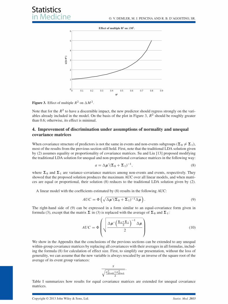
Figure 3. Effect of multiple R2 on �M 2.

Note that for the R2 to have a discernible impact, the new predictor should regress strongly on the vari-ables already included in the model. On the basis of the plot in Figure 3, R2 should be roughly greaterthan 0.6; otherwise, its effect is minimal.

4. Improvement of discrimination under assumptions of normality and unequalcovariance matrices

When covariance structure of predictors is not the same in events and non-events subgroups (†0 ¤†1/,most of the results from the previous section still hold. First, note that the traditional LDA solution givenby (2) assumes equality or proportionality of covariance matrices. Su and Liu [13] proposed modifyingthe traditional LDA solution for unequal and non-proportional covariance matrices in the following way:

aD��0.†0C†1/�1; (8)

where †0 and †1 are variance–covariance matrices among non-events and events, respectively. Theyshowed that the proposed solution produces the maximum AUC over all linear models, and when matri-ces are equal or proportional, their solution (8) reduces to the traditional LDA solution given by (2).

A linear model with the coefficients estimated by (8) results in the following AUC:

AUC Dˆ�p

��0.†0C†1/�1��: (9)

The right-hand side of (9) can be expressed in a form similar to an equal-covariance form given informula (3), except that the matrix † in (3) is replaced with the average of †0 and †1:

AUC Dˆ

0BB@vuut��0

�†0C†1

2

��1��

2

1CCA (10)

We show in the Appendix that the conclusions of the previous sections can be extended to any unequalwithin-group covariance matrices by replacing all covariances with their averages in all formulas, includ-ing the formula (8) for calculation of effect size. First, to simplify our presentation, without the loss ofgenerality, we can assume that the new variable is always rescaled by an inverse of the square root of theaverage of its event group variances:

xq�2DD0

C�2DD1

2

:

Table I summarizes how results for equal covariance matrices are extended for unequal covariancematrices.



Table I. Summary of factors that improve model performance.

Factors that improve model performance for

Equal covariance matrices Unequal covariance matrices

1. cov.xp ; rsp�1/ < 0 1. cov.xp ;rsp�1/DD0Ccov.xp ;rsp�1/DD12 < 0

2. High multiple R2 of regressing xp on .x1; : : :; xp�1/. 2. High modified R2 – see Appendix for the formula.3. High ıp provided ıp > cov.xp ; rsR/ 3. High ıp provided

ıp >cov.xp ;rsp�1/DD0Ccov.xp ;rsp�1/DD1

2

covDD0.xp , rsR/ and covDD1.xp , rsR/ is covariance between new predictor and the old risk score calculated sepa-rately among non-events and events, respectively, ıp is effect size calculated with respect to the average of variances:

ıp D��2q

varDD0.xp/CvarDD1.xp/2

D��2pvar.xp/

.

5. Connection between covariance matrices conditional on event status andunconditional covariance matrix

Results of the previous sections were formulated in terms of covariance matrices of the predictorsconditional on event status. However, we want to stress that conditional matrices are different fromcovariance matrix of the predictors calculated in the whole sample (also called unconditional variance–covariance matrix). In this section, we discuss the difference between the two types of matrices andhow it affects our results. In a bivariate case (p D 2), if the matrices are equal, a negative correlationbetween predictors remains beneficial even if it is calculated in the whole sample (unconditional). In theAppendix, we show that when the number of predictors p D 2 and the conditional matrices are equal,the within-group � of Section 2 is a linearly increasing function of �uncond. and negative �uncond. alsoleads to an improvement in the AUC. In Figure 4, we plot the AUC as a function of conditional andunconditional �.

Figure 4 shows that, in general, the two correlations are different even in this simple case of a bivari-ate model with equal covariance matrices. This figure illustrates that general relationships discussed inprevious sections from conditional case hold in the unconditional case. However, in the case of morethan two predictor variables, there is no clear relationship, and it is not possible to explicitly write thefunctional form when the matrices are unequal (see more details in the Appendix). This means that, ingeneral, there is a fundamental difference between the two definitions, and to correctly apply the resultsof this paper, one must operate with conditional covariance matrices.

6. Application to Framingham Heart Study data and simulations

We use the Framingham Heart Study data to illustrate our findings from the previous sections. In par-ticular, we will show situations where negative and high positive correlations are beneficial for discrim-ination. A total of 8365 observations on people free of cardiovascular disease at a baseline examination

AU

C

conditional and unconditional

AUC as a function of conditional and unconditional

δ2=.1 unconditional

δ2=.1 condotional


δ2=.5 conditional


δ2=.74 conditional

Figure 4. AUC as a function of conditional and unconditional correlation between new and old predictors fordifferent effect sizes.



in the 1970s were available. Measurements of risk factors and results of medical tests were obtained,including age, total and HDL cholesterol (tot and hdl), and systolic and diastolic blood pressure (sbpand dpf). Participants of the study were followed up for 12 years for the development of CHD and werecategorized as cases if they developed CHD or non-cases if they did not. To correct for skewness of thepredictors, simple logarithmic transformations were applied. The resulting distributions were unimodalwith moderate degree of skewness; however, normality could still be rejected using the Shapiro–Wilkstest [17, 18]. We present the average of the two correlation matrices of the transformed predictors andunivariate effect sizes in Table II.

To mimic an analysis most likely to occur in practical applications, we applied logistic regression toanalyze this data. Suppose we build a model ‘from scratch’. First, we select ln age because it has thelargest univariate effect size (0.72). Then, a common strategy would suggest adding ln sbp, because it hassecond largest effect size (0.62). Addition of ln sbp increases the AUC from 0.690 to 0.713. However,using the results of Section 2, we should consider variables negatively correlated with age, namely lnhdl. This variable has a much smaller effect size (0.46), yet its correlation with age is negative (�0:09).The model with ln age and ln hdl has an AUC of 0.734, clearly better than the AUC of the model basedon ln age and ln sbp. One might argue that ln sbp has a stronger correlation with ln age than ln hdl,so this is why the less correlated ln hdl improves discrimination by a larger amount. To illustrate thatnegative correlation with variables already in the model is beneficial for the improvement in the AUC,we looked at the impact of a variable with the same effect size as ln hdl and the same in magnitudebut opposite in direction correlation with ln age. Ln age has the same strength of correlation with lndpf as with as ln hdl but with the opposite sign: 0.09 versus �0:09. So ln dpf is a good candidate toillustrate the main idea. It has a smaller effect size than ln hdl, so we added a constant to it in the dis-order group to match the effect size of ln hdl. Although modified ln dpf now has the same effect sizeas ln hdl and a similar in magnitude but opposite in direction correlation with ln age, it results in theAUC of 0.716, still considerably smaller than the AUC of 0.734 obtained using the negatively correlatedln age and ln hdl. This illustrates that the negative correlation of ln hdl must play an important role inthis example.

To proceed further with model building, we should find new variables that are negatively correlatedwith the risk score (linear combination of ln age and ln hdl) and/or have a very high modified multipleR-squared. In the data described earlier, we do not have such variables. So we decided to keep the real-life ln age and ln hdl but simulate several versions of the candidate new variables. We created the newvariables as linear combinations of ln age and ln hdl plus a random normal term. We kept the effect sizeof the new predictor fixed at 0.60 and varied its correlation with the risk score based on the model with lnage and ln hdl. We present the AUCs of the model with ln age, ln hdl, and the theoretical new predictorin Table III (recall that the AUC of the model with ln age and ln hdl is 0.734).

Table III illustrates how the predictor that leads to the highest improvement in discrimination iseither negatively associated with original risk score (�0:70 in row 2) or regressed on the existing vari-ables with a very high multiple R2 (0.91 in row 4). The new predictor that is uncorrelated with theexisting ones in terms of R2 (0.00 in row 1) produces a much smaller AUC (0.789) than the nega-tively associated predictor (0.869) or the predictor with a very large R2 (AUC of 0.942). However, therelationship with R2 is non-monotonic – looking at row 3, we notice that not sufficiently large R2 isa disadvantage.

Table II. Average of the two correlation matrices of the transformed predictorsand univariate effect sizes.

Predictor ln age ln dpf ln sbp ln hdl* ln tot(effect size) (0.72) (0.42) (0.62) (0.46) (0.49)

ln age 1.0 0.09 0.41 �0:09 0.25ln dpf 1.0 0.67 0.06 0.11ln sbp 1.0 �0:01 0.15ln hdl* 1.0 �0:10

ln tot 1.0

To satisfy assumption of non-negative effect size, ln hdl was multiplied by �1 anddenoted as ln hdl*.



Table III. Impact of correlation on predictive ability of a new (third) biomarker.

Type of new predictor Univariate effect size Correlation with the old risk score R2 AUC

Uncorrelated 0.60 0.05 0.00 0.789Negatively correlated 0.60 �0:70 0.54 0.869Positively correlated I 0.60 0.73 0.58 0.766Positively correlated II 0.60 0.91 0.91 0.942

AUC is 0.734 for the baseline model with two predictors ln age and ln hdl.

When we have repeated analysis presented in Section 6 for training (80% of the data) and valida-tion (20% of the data) datasets, values of the AUC changed only slightly (second decimal place), andall conclusions of Section 6 remained the same (tables are available online as Web-based Supportinginformation)‡.

7. Discussion

In this paper, we prove that for normally distributed data, negative correlation between two predictorsis better than zero correlation in terms of discrimination between events and non-events. Furthermore,in some settings, a new predictor that is highly correlated with the existing predictors can also lead tolarger gains in discrimination.

We chose the AUC as a measure of discrimination, but the observed behavior of new predictors isnot a function of this choice. It should remain true for any sensible measure of discrimination. This canbe seen from the following plots in Figure 5. In this figure, we present a number of scatterplots of xversus y that represent two multivariate normal random variables with conditional distributions givenby (x;y/jD D 0 � N.0;†) and (x;y/jD D 1 � N.ı, †). We consider ı D .1:5; 0:6/ and differentvariance–covariance matrices †, which lead to conditional (on D) correlations � equal to 0, �0:85, and0.98. Events (D D 1) are marked as dots and non-events (D D 0) as circles. We note that for �D 0 dotsand circles form two round clouds with substantial overlap. As � changes, the two clouds become ellip-soidal, and for � D �0:85, we see almost compete separation between them. We need a higher positivecorrelation in order to achieve the same effect of almost perfect separation. The scatterplot for �D 0:98demonstrates a separation comparable with what is seen when �D�0:85.

This topic has been studied before. Mardia et al. [15] observed that correlation improved discrimi-nation in the bivariate normal case. Cochran [16] discussed the same issue, but both did it in terms ofthe probability of misclassification. Our paper addresses how those results are related to the improve-ment in model discrimination as quantified by the AUC and extends the earlier results to the multivariatenormal case and unequal covariance matrices. Further research is needed to extend these results rigor-ously beyond normality. However, it can be argued that any continuous predictor can be transformedto have its distribution approximate normality, so our assumption is not prohibitively restrictive in thiscase. Furthermore, our example using Framingham Heart Study data with variables that were not normalsuggested that the results seem to hold if normality is not grossly violated. This suggestion needs to beverified by simulations.

It is essential to note that our findings are theoretical in nature and they intend to point out that thecorrelation and effect size between the new predictor and the existing variables have a more compli-cated relationship with improvement in discrimination. The popular notion that no correlation and higheffect size offer all that we need is not true. However, this simple notion may not be far off from thetruth, when we are willing to restrict our attention to non-negative correlations and sufficiently largeeffect sizes. We see in Figure 1 that for effect sizes of 0.5 or 0.74 and correlations between 0 and0.6, the improvement in discrimination decreases as a function of correlation. On the other hand, inFigure 2, we observe that for correlations that are not overly large, the improvement increases as a func-tion of effect size. These effect sizes and limited correlations are the most likely scenarios occurringin practice.

‡Supporting information may be found in the online version of this article.



Figure 5. Scatterplots of x1 and x2 for different correlations between x1 and x2. Pluses are events and circlesare non-events.

Our findings, however, offer new directions in the search for novel predictors. Although it may beextremely difficult to identify variables with extremely large correlations and different effect sizes (wehad to simulate them ourselves), finding predictors with negative correlation need not be as formidable.As seen in our example with hdl, even small amount of negative correlation can lead to a noticeableimprovement in discrimination. Thus, identification of predictors that correlate negatively with the exist-ing risk factors and retain sufficient strength of association with the outcome may be the most promisingdirection in the search for new markers.

Appendix

Notation. A disease status D and p medical test results are available for N patients. We denote testresults as x D x1; : : : ; xp . We assume multivariate normality of test results conditional on the diseasestatus: xjD D 0 � N.�0, †0/ and xjD D 1 � N.�1, †1/, where �0 and �1 are vectors of meansfor the p test results among non-events and events, respectively, and †0 and †1 are the variance–covariance matrices of the predictor in the subgroups of non-events and events correspondingly. Wefurther denote differences in group means between events and non-events as��D �1��0 and assumethat mean differences are all non-negative: �� > 0. Our goal is to evaluate improvement in the AUCafter adding the pth variable to the first p�1 variables. We can write any variance–covariance matrix†

as† D

�†11†12†21†22

�, where†11 is the variance–covariance matrix for the first p�1 predictors,†12 is

the covariance matrix of the first p � 1 predictors with the new predictor and †22 is the variance of the

new predictor.�� can be written as

��1��2

�, where��1 is the vector of differences in the means of

the first p � 1 predictors and ��2 is the difference of means of the new predictor.



Part 1. Equal variance–covariance matrices (†0 D†1 D†)

A1. Mahalanobis Distance decomposition [15]

Using the notation of Section 2, the Mahalanobis distance of the full model based on all p predictors�M 2p

can be written as a function of the corresponding distance for the first p � 1 variables

�M 2p�1

�plus an increment .�M 2/:

M 2p D��

0†�1��D��0

1†�111��1

C��2 �†21†

�111��1

0 �†22 �†21†

�111†12

�1 ��2 �†21†

�111��1

DM 2

p�1C�M2;

where

�M 2 D��2 �†21†

�111��1

0 �†22 �†21†

�111†12

�1 ��2 �†21†

�111��1

(A1)

A2. �M 2 when p D 2

When p D 2, then we can simplify (A1) because †11 D var x1, †22 D var x2, †12 D cov.x1; x2/:

�M 2

��2 �

cov.x1;x2/var x1

��1

�2var x2 �

cov2.x1;x2/var x1

D.ı2 � �ı1/

2

1� �2; (A2)

where �D corr.x1; x2/.Therefore, improvement in the AUC is fully defined by (A2), which is a function of effect size and

correlation coefficient of the old and new predictor variables.

A3. Conditions of improvement in AUC when p D 2

Let us investigate the behavior of �M 2 defined in (A2) as function of � and effect size ı2.

Improvement in AUC as a function of �. The first derivative of �M 2 with respect to � is as follows:

.�M 2/0� D

.ı2 � ı1�/

2

1� �2

!0�

D2.ı2 � ı1�/.ı2�� ı1/

.1� �2/2

There are two possible cases:

Case 1. ı2 ¤ ı1

The first derivative is zero when �D

ı1=ı2, if ı1 < ı2ı2=ı1, if ı2 < ı1

and changes sign from negative to positive

as we approach the root from left to right. Therefore, �M 2 is a convex function with a minimum at thespecified values of �. Minimum is attained at the positive value of �, and hence any negative � is betterfor discrimination than �D 0.

Case 2. ı2 D ı1 D ı

In this case, �M 2 reduces to the following:

�M 2 D.ı2 � ı1�/

2

1� �2Dı2.1� �/

1C �

Its first derivative is equal to �2ı2

.1C�/2, and it is always negative. Therefore, �M 2 is a decreasing

function of �.Therefore, the following statements describe improvement in discrimination as measured by�M 2:

1. If ı1 ¤ ı2, then �M 2 is convex in terms of �. It achieves its minimum at � D ı2=ı1 or � D ı1=ı2(if ı2 < ı1 or ı1 < ı2, correspondingly) and achieves its maximum as �!˙ 1.



2. If ı1 D ı2, then �M 2 is monotone decreasing in �.3. If � <0 as �!�1, both numerator and denominator contribute to the growth of �M 2. Indeed, as� becomes closer to �1, the numerator is increasing, and the denominator is decreasing, which cre-ates synergistic effect on the growth of�M 2. This is different when � >0. As positive � increases,both the denominator and numerator decrease. Therefore, any negative correlation is beneficial, andalso �M 2 improves at a faster rate for negative correlation than for positive correlation.

Improvement in AUC as a function of effect size of new predictor. Let us investigate the behavior of

function �M 2 D .ı2�ı1�/2

1��2as a function of the effect size of the new predictor ı2. �M 2 is a quadratic

function with respect to ı2 with the minimum attained at ı2 D ı1�. If ı2 < ı1�, the derivative of �M 2

with respect to ı2 is negative, and we observe a paradoxical behavior when�M 2 is a decreasing functionof the effect size of the new variable, and a larger effect size ı2 translates into a smaller improvement inthe AUC. We illustrate this unexpected behavior in Figure 2. If ı2 > ı1�, then the derivative is positive,and the larger effect size is beneficial.

A4. Improvement in AUC when p > 2

Without loss of generality, we can assume that the new predictor xp has a unit variance. Therefore,†22 D 1 and the difference of means of the new variable equals its effect size, ��2 D ıp .

Statement. When p > 2,�M 2 D.ıp�cov.xp ; rsp�1//

2

1�R2, where cov.xp; rsp�1/ is the covariance between

the new predictor and the old risk score from the model based on the first p � 1 variables and R2

is the coefficient of determination from a multiple regression of xp on x1,. . . , xp�1 conditional onevents status.

ProofIndeed, when p > 2, �M 2 can be written as follows:

�M 2 D

�ıp �†21†

�111��1

21�†21†

�111†12

(A3)

We note that if rsp�1 is the risk score based on the reduced model, then

cov.xp; rsp�1/D cov�xp; ��

01†�111 .x1; : : : ; xp�1/

0D��01†

�111 cov.xp; .x1; : : : ; xp�1/

0/

D��01†�111†12 D†21†

�111��1

(A4)

Also 1�†21†�111†12 D 1�R

2, see [19].Hence, we can rewrite (A1) as follows:

�M 2 D.ıp � cov.xp; rsp�1//2

1�R2

�

Part 2. Unequal variance–covariance matrices

A5. Mahalanobis distance decomposition when †0 ¤†1

Su and Liu’s solution [13], a D ��0.†0 C†1/�1, is optimal for linear models when predictors have

different variance–covariance structure in event and non-event groups. This solution produces AUC that

can be written as in (8): AUC D�p

��0.†0C†1/�1��

. We still can apply Mahalanobis distance

decomposition to��0.†0C†1/�1�� as was shown in the Appendix of [20]. Therefore, improvement



in the AUC is again fully defined by the improvement in the�M 2, which can be written in the followingway:

M 2p D��

0 N†�1��D

��1��2

�0 � N†11 N†12N†21 N†22

��1 ��1��2

�

D��0

1N†�1

11��1C��2 �

N†21 N†�1

11��1

�0 �N†22 � N†21 N†

�1

11N†12

��1��2 �

N†21 N†�1

11��1

�DM 2

p�1C�M2;

where N†ij D†DD0ij C†DD1ij

2i; j D 1; 2

To simplify calculations, we assume that the new predictor is rescaled by the inverse of the aver-age of the two within-group variances. Therefore, without the loss of generality, we can assume that†22 D 1. Because within-group matrices are unequal, we suggest defining effect size as the ratio of

mean difference to the square of the average variance:p

var xp Dq

varDD0 xpCvarDD1 xp2

. Then, themean difference of the rescaled new predictor and its effect size are equal: ��2 D ıp . Therefore, wecan write �M 2 as follows:

�M 2 D�ıp � N†21 N†

�1

11��1

�0 �1� N†21 N†

�1

11N†12

��1 �ıp � N†21 N†

�1

11��1

�(A5)

A6. Improvement in AUC when p D 2

When p D 2, N†12 D 12.cov.x1; x2/DD0C cov.x1; x2/DD1/D cov.x1; x2/, and we can rewrite (A5) as

�M 2 D .ı2�ı1cov.x1;x2//2

1�cov2.x1;x2/.

A7. Conditions for improvement of AUC when p D 2

All conclusions of A3 hold for unequal covariance matrices once � is replaced with cov.x1; x2/.

A8. Improvement of AUC when p > 2

Statement.

If p > 2;�M 2 D

�ıp �

cov.xp ;rsp�1/DD0Ccov.xp ;rsp�1/DD12

�21�R2�

; (A6)

where R2� D N†21 N†�1

11N†12.

ProofWhen p > 2 �M 2 in (A5) can be written as follows:

�M 2 D

�ıp � N†21 N†

�1

11��1

�21� N†21 N†

�1

11N†12

(A7)

Let us show that N†21 N†�1

11��1 D cov.xp; rsp�1/. Conditioning on non-events groups, we can writethe following:

cov0.xp; rsp�1/D cov0.xp; ��0 N†�1

11 .x1; : : : ; xp�1/0/D��01

N†�1

11 cov0.xp; .x1; : : : ; xp�1/0/

D��01N†�1

11†DD012 D†DD021

N†�1

11��1:

Similarly among events, cov1.xp; rsp�1/D†DD121N†�1

11��1.

Thus, cov0.xp ;rsp�1/Ccov1.xp ;rsp�1/2

D.†DD021 C†DD121 /

2N†�1

11��1defD N†21 N†

�1

11��1.

1 � N†21 N†�1

11N†12 in the denominator of (A7) resembles formula (A4) for multiple regression R2,

except the covariance matrices in it should be replaced by the average of covariance matrices in the twosubgroups. So by analogy to (A3), we define it as R2� – modified multiple R2.



Hence, we can rewrite (A7) as follows:

�M 2 D

�ıp � cov.xp; rsp�1/

�21�R2� �

A9. Correlation conditional on event status versus correlation calculated among non-events and eventspooled together

If a model has two predictors with equal covariance structure within event and non-event categories,there exists a relationship between the two types of covariances.

Let

�x1x2

�DD0

�N

�0;

��21�12�12�

22

��;

�x1x2

�DD1

�N

��1��2

�;

"�21�12�12�

22

#!Denote the fraction of events as � and EDD0 D E0, EDD1 D E1. The covariance calculated in a

sample that pools events and non-events is as follows:

cov.x1; x2/DE.x1x2/�Ex1Ex2

Because E0.x1x2/D �12 and E1.x1x2/D �C12��1��2;

E.x1x2/D .1� �/E0.x1x2/C �E1.x1x2/D �12C ��1��2

Ex1Ex2 D �2��1��2

So cov.x1; x2/D �12C �.1� �/��1��2

Because var x1 D �21 C �.1� �/��21; var x2 D �22 C �.1� �/��

22,

�mixed D�12C �.1� �/��1��2

pvar x1var x2

D�C �.1� �/ı1ı2p

.1C �.1� �/ı1/.1C �.1� �/ı2/; (A8)

where �DD0 D �DD1 D � is the correlation coefficient between x1 and x2 conditional on event status. Itfollows from (A8) that unconditional correlation is a linear increasing function of within-group correla-tion coefficient �. However, there is no such clear relationship when the number of predictors is greaterthan two nor for unequal covariance matrices.

References1. Wilson PWF, D’Agostino RB, Levy D, Belanger AM, Silbershatz H, Kannel WB. Prediction of coronary heart disease

using risk factor categories. Circulation 1998; 97:1837–1847.2. Anderson KM, Odell PM, Wilson PWF, Kannel WB. Cardiovascular disease risk profiles. American Heart Journal 1991;

121:293–298.3. D’Agostino RB, Vasan RS, Pencina MJ, Wolf PA, Cobain MR, Massaro JM, Kannel WB. General cardiovascular risk

profile for use in primary care: the Framingham Heart Study. Circulation 2008; 117:743–753.4. Grundy SM, Becker D, Clark LT, Cooper RS, Denke MA, Howard WJ. Executive summary of the third report of the

National Cholesterol Education Program (NCEP) expert panel on detection, evaluation and treatment of high bloodcholesterol in adults (Adult Treatment Panel III). Journal of the American Medical Association 2001; 285:2486–2497.

5. Gail MH, Brinton LA, Byar DP, Corle DK, Green SB, Schairer C, Mulvihill JJ. Projecting individualized probabilities ofdeveloping breast cancer for white females who are being examined annually. Journal of the National Cancer Institute1989; 81:1879–1886.

6. Gail MH, Costantino JP, Pee D, Bondy M, Newman L, Selvan M, Anderson GL, Malone KE, Marchbanks PA,McCaskill-Stevens W, Norman SA, Simon MA, Spirtas R, Ursin G, Bernstein L. Projecting individualized absoluteinvasive breast cancer risk in African American women. Journal of the National Cancer Institute 2007; 99(23):1782–1792.

7. Golub TR, Slonim DK, Tamayo P, Huard C, Gaasenbeek M, Mesirov JP, Coller H, Loh ML, Downing JR, Caligiuri MA,Bloomfield CD, Lander ES. Molecular classification of cancer: class discovery and class prediction by gene expressionmonitoring. Science 1999; 286(5439):531–537.

8. Pepe MS. The Statistical Evaluation of Medical Tests for Classification and Prediction. Oxford University Press: NewYork, 2004, 77–79.

9. D’Agostino RB, Griffith JL, Schmidt CH, Terrin N. Measures for evaluating model performance. In Proceedings of theBiometrics Section. American Statistical Association, Biometrics Section: Alexandria, VA. U.S.A., 1997; 253–258.

10. Harrel FE. Tutorial in biostatistics: multivariable prognostic models: issues in developing models, evaluating assumptionsand adequacy, and measuring and reducing errors. Statistics in Medicine 1996; 15:361–387.

11. Bamber D. The area above the ordinal dominance graph and the area below the receiver operating characteristic graph.Journal of Mathematical Psychology 1975; 12:387–415.



12. Hanley JA, McNeil BJ. The meaning and use of the area under a receiver operating characteristic (ROC) curve. Radiology1982; 143:29–36.

13. Su JQ, Liu JS. Linear combinations of multiple diagnostic markers. Journal of American Statistical Association 1993;88(424):1350–1355.

14. Efron B. The efficiency of logistic regression compared to normal discriminant analysis. Journal of American StatisticalAssociation 1973; 70(352):892–898.

15. Mardia KV, Kent JT, Bibby JM. Multivariate Analysis. Academic Press: San Diego, 1979.16. Cochran WG. On the performance of the linear discriminant function. Technometrics 1964; 6(2):179–190.17. Shapiro SS, Wilk MB. An analysis of variance test for normality (complete samples). Biometrika 1965; 52(34):591–611.18. Pearson ES, D’Agostino RB, Bowman RO. Tests for departure from normality comparison of powers. Biometrika 1977;

64(2):231–246.19. Weisberg S. Applied Linear Regression. John Wiley and Sons: New Jersey, 2005, 62–64.20. Demler OV, Pencina MJ, D’Agostino RB Sr. Equivalence of improvement in area under ROC curve and linear discriminant

analysis coefficient under assumption of normality. Statistics in Medicine 2011; 30(12):1410–1418.


impact of correlation on predictive ability of biomarkers

Documents