Atmos. Chem. Phys., 12, 11329–11337, 2012www.atmos-chem-phys.net/12/11329/2012/doi:10.5194/acp-12-11329-2012© Author(s) 2012. CC Attribution 3.0 License.

AtmosphericChemistry

and Physics

Impact of 2000–2050 climate change on fine particulate matter(PM2.5) air quality inferred from a multi-model analysis ofmeteorological modes

A. P. K. Tai, L. J. Mickley, and D. J. Jacob

School of Engineering and Applied Sciences, Harvard University, Cambridge, Massachusetts, USA

Correspondence to:A. P. K. Tai (pkamostai@gmail.com)

Received: 6 June 2012 – Published in Atmos. Chem. Phys. Discuss.: 20 July 2012Revised: 5 November 2012 – Accepted: 24 November 2012 – Published: 3 December 2012

Abstract. Studies of the effect of climate change on fineparticulate matter (PM2.5) air quality using general circula-tion models (GCMs) show inconsistent results including inthe sign of the effect. This reflects uncertainty in the GCMsimulations of the regional meteorological variables affect-ing PM2.5. Here we use the CMIP3 archive of data from fif-teen different IPCC AR4 GCMs to obtain improved statisticsof 21st-century trends in the meteorological modes drivingPM2.5 variability over the contiguous US. We analyze 1999–2010 observations to identify the dominant meteorologicalmodes driving interannual PM2.5 variability and their syn-optic periods T. We find robust correlations (r > 0.5) of an-nual mean PM2.5 with T, especially in the eastern US wherethe dominant modes represent frontal passages. The GCMsall have significant skill in reproducing present-day statisticsfor T and we show that this reflects their ability to simulateatmospheric baroclinicity. We then use the local PM2.5-to-period sensitivity (dPM2.5/dT) from the 1999–2010 observa-tions to project PM2.5 changes from the 2000–2050 changesin T simulated by the 15 GCMs following the SRES A1Bgreenhouse warming scenario. By weighted-average statis-tics of GCM results we project a likely 2000–2050 increaseof ∼ 0.1 µg m−3 in annual mean PM2.5 in the eastern US aris-ing from less frequent frontal ventilation, and a likely de-crease albeit with greater inter-GCM variability in the Pa-cific Northwest due to more frequent maritime inflows. Po-tentially larger regional effects of 2000–2050 climate changeon PM2.5 may arise from changes in temperature, biogenicemissions, wildfires, and vegetation, but are still unlikely toaffect annual PM2.5 by more than 0.5 µg m−3.

1 Introduction

Air pollution is strongly sensitive to weather conditions andis therefore affected by climate change. A number of stud-ies reviewed by Jacob and Winner (2009) have used chem-ical transport models (CTMs) driven by general circulationmodels (GCMs) to diagnose the effects of 21st-century cli-mate change on air quality at northern mid-latitudes. TheseGCM-CTM studies generally concur that 2000–2050 climatechange will degrade ozone air quality in polluted regions by1–10 ppb, but they do not agree on even the sign of the ef-fect for fine particulate matter (PM2.5). Change in ozone islargely driven by change in temperature, but for PM2.5 thedependence on meteorological variables is far more complex,including different sensitivities for different PM2.5 compo-nents (Liao et al., 2006; Dawson et al., 2007; Heald et al.,2008; Kleeman, 2008; Pye et al., 2009; Tai et al., 2010).

Tai et al. (2012) proposed an alternate approach for diag-nosing the effect of climate change on PM2.5 through iden-tification of the principal meteorological modes driving ob-served PM2.5 variability. For example, it is well known thatcold fronts associated with mid-latitude cyclones drive pol-lutant ventilation in the eastern US (Cooper et al., 2001; Liet al., 2005). Tai et al. (2012) found that the frequency ofcold fronts was a major predictor of the observed interannualvariability of PM2.5 in the Midwest. GCMs project a gen-eral 21st-century decrease in mid-latitude cyclone frequencyas a result of greenhouse warming (Bengtsson et al., 2006;Lambert and Fyfe, 2006; Christensen et al., 2007; Pinto etal., 2007; Ulbrich et al., 2008), from which one could de-duce a general degradation of air quality. This cause-to-effect

Published by Copernicus Publications on behalf of the European Geosciences Union.

11330 A. P. K. Tai et al.: Impact of climate change on PM2.5 air quality

relationship has been found in a few GCM-CTM studies(Mickley et al., 2004; Murazaki and Hess, 2006).

However, there is substantial uncertainty in regional pro-jections of future cyclone frequency (Ulbrich et al., 2009;Lang and Waugh, 2011). Indeed, a general difficulty in pro-jecting the effect of climate change on air quality is theunderlying GCM uncertainty in simulating regional climatechange. This uncertainty arises both from model noise (cli-mate chaos) and from model error (physics, parameters, nu-merics). Model noise can be important. Tai et al. (2012) con-ducted five realizations of 2000–2050 climate change in theGISS GCM 3 (Rind et al., 2007) under the same radiativeforcing scenario and found that the frequency of cyclonesventilating the US Midwest decreased in three of the realiza-tions, increased in one, and had no trend in one. All GCM-CTM studies to date examining the effect of climate changeon PM2.5 have used a single climate change realization froma single GCM (Jacob and Winner, 2009), so it is no sur-prise that they would yield inconsistent results. This is lessof an issue for GCM-CTM projections of ozone air qualitybecause ozone responds most strongly to changes in temper-ature (Jacob and Winner, 2009), and all GCMs show consis-tent warming for the 21st-century climate even on regionalscales (Christensen et al., 2007).

The standard approach adopted by the Intergovernmen-tal Panel on Climate Change (IPCC) to reduce uncertain-ties in GCM projections of regional climate change is to usemultiple realizations from an ensemble of GCMs, assum-ing that model diversity provides some measure of modelerror (Christensen et al., 2007). Such an ensemble analy-sis is not practical for GCM-CTM studies of air quality be-cause of the computational expense associated with chem-istry and aerosol microphysics. An alternative is to focus onGCM projections of the meteorological modes determiningair quality. A resource for this purpose is the World Cli-mate Research Programme’s (WCRP’s) Coupled Model In-tercomparison Project phase 3 (CMIP3) multi-model datasetof 2000–2100 climate change simulations produced by theensemble of GCMs contributing to the IPCC 4th AssessmentReport (AR4).

Here we use this multi-model ensemble to project theresponses of PM2.5 air quality in different US regions to2000–2050 climate change. We focus on annual mean PM2.5,which is of primary policy interest (EPA, 2012). We first ex-amine the observed sensitivity of annual mean PM2.5 to thefrequencies of the dominant meteorological modes in differ-ent US regions. We then use the CMIP3 archive of 15 GCMsto project the effect of climate change on these frequencies,and from there we deduce the corresponding effect of climatechange on PM2.5.

2 Observed sensitivity of PM2.5 to meteorologicalmodes

Previous studies have demonstrated the importance of syn-optic weather in controlling PM2.5 variability (Thishan Dhar-shana et al., 2010; Tai et al., 2012). Tai et al. (2012) identi-fied cyclone passage with associated cold front as the me-teorological mode whose period T (length of one cycle,i.e., inverse of frequency) is most strongly correlated withinterannual variability of PM2.5 in the US Midwest. Theyproposed that the corresponding PM2.5-to-period sensitivity(dPM2.5/dT) could be used to project the response of PM2.5to future climate change; a change1T in cyclone periodwould cause a change1PM2.5 = (dPM2.5/dT)1T . This as-sumes that the local dPM2.5/dT relationships will remain un-changed, and that the same meteorological modes will re-main dominant for PM2.5 variability. The physical meaningof dPM2.5/dT is clear when the meteorological mode acts asa pulse, either ventilating a source region (as in the case of acold front) or polluting a remote region (as in the case of awarm front).

Daily mean PM2.5 data for 1999–2010 were obtained fromthe EPA Air Quality System (AQS) (http://www.epa.gov/ttn/airs/airsaqs/) Federal Reference Method (FRM) network ofabout 1000 sites in the contiguous US. The daily site mea-surements were interpolated following Tai et al. (2010) ontoa 4◦

× 5◦ latitude-by-longitude grid, and annual means foreach of the 12 yr were calculated for each grid cell. Such spa-tial averaging can smooth out local effects and yields morerobust correlation statistics of PM2.5 with synoptic weather(Tai et al., 2012). Figure 1 shows as an example the 1999–2010 time series of annual mean PM2.5 for the 4◦ × 5◦ gridcell centered over Chicago (asterisk in Fig. 2). Linear regres-sion indicates a downward trend of−0.34 µg m−3 a−1, re-flecting the improvement of air quality due to emission con-trols (EPA, 2012). Superimposed on this long-term trend isinterannual variability that we assume to be meteorologicallydriven. The standard deviation of the detrended annual meanPM2.5 is 0.79 µg m−3, or 5.3 % of the 12-yr mean PM2.5. Forthe ensemble of 4◦ × 5◦ grid cells in the US we find that theinterannual standard deviation of the detrended data rangesfrom 3 to 19 % of 12-yr mean PM2.5. Relative interannualvariability is largest in the western US but there it could bedriven in part by forest fires (Park et al., 2007).

We follow the approach of Tai et al. (2012) to deter-mine the dominant meteorological modes for interannualPM2.5 variability on the 4◦ × 5◦ grid. Daily meteorologi-cal variables for 1981–2010 (Table 1) were obtained fromthe National Center for Environmental Prediction/NationalCenter for Atmospheric Research (NCEP/NCAR) Reanal-ysis 1 (http://www.esrl.noaa.gov/psd/data/gridded/data.ncep.reanalysis.html) (Kalnay et al., 1996; Kistler et al., 2001). Weregridded the original 2.5◦ × 2.5◦ data onto the 4◦ × 5◦ gridand deseasonalized them by subtracting the 30-day movingaverages.

Atmos. Chem. Phys., 12, 11329–11337, 2012 www.atmos-chem-phys.net/12/11329/2012/

A. P. K. Tai et al.: Impact of climate change on PM2.5 air quality 11331

Table 1. Variables used to define meteorological modes for PM2.5variabilitya.

Variable Description

x1 Surface air temperature (K)b

x2 Surface air relative humidity (%)b

x3 Precipitation rate (mm d−1)

x4 Sea level pressure (hPa)x5 Sea level pressure tendency dSLP/dt (hPa d−1)

x6 Surface wind speed (m s−1)b,c

x7 East-west wind direction indicator cosθ (dimensionless)d

x8 North-south wind direction indicator sinθ (dimensionless)d

a From the National Center for Environmental Prediction/National Center forAtmospheric Research (NCEP/NCAR) Reanalysis 1 for 1981–2010. All data are24-h averages and are deseasonalized as described in the text.b “Surface” data are from 0.995 sigma level.c Calculated from the horizontal wind vectors (u, v).d θ is the angle of the horizontal wind vector counterclockwise from the east.Positive values ofx7 andx8 indicate westerly and southerly winds, respectively.

Fig. 1. Observed 1999–2010 time series of annual mean PM2.5and synoptic period T of the dominant meteorological mode (coldfrontal passage) for the 4◦

× 5◦ grid square centered over Chicagoat 42◦ N, 87.5◦ W (asterisk in Fig. 2). Linear regression lines areshown as dashed. The detrended variables have a correlation ofr = 0.62.

Following Tai et al. (2012), we decomposed the dailytime series of the meteorological variables (Table 1) for each4◦

× 5◦ grid cell to produce time series of eight principalcomponents (U1, ...,U8):

Uj (t) =

8∑k=1

αkj

xk(t) − xk

sk(1)

wherexk is the deseasonalized meteorological variable,xk

andsk are the temporal mean and standard deviation ofxk,αkj describes the elements of the orthogonal transformationmatrix defining the meteorological modes (Tai et al., 2012),andt is time. EachUj (t) represents the principal componenttime series for a distinct meteorological mode. We then ap-plied Fourier transform toUj (t) with a second-order autore-gressive (AR2) filter to obtain a smoothed frequency spec-trum for each year (Wilks, 2011), and extracted the medianAR2 spectral frequency (f ) to calculate the correspondingperiod of the meteorological mode (T= 1/f ). See Tai etal. (2012) for further description and example application, in-

Fig. 2. Interannual correlation of annual mean PM2.5 with the pe-riod T of the dominant meteorological mode for 1999–2010 ob-servations: correlation coefficients (top) and reduced-major-axis re-gression slopes dPM2.5/dT (bottom). Only values significant with90 % confidence (p-value< 0.1) are shown. The asterisk marks theChicago grid cell for which the time series of PM2.5 and T areshown in Fig. 1.

cluding justification for extracting median frequency insteadof mean.

From there we applied reduced major axis regression tothe 1999–2010 annual time series of detrended PM2.5 andT in each 4◦ × 5◦ grid cell to determine dPM2.5/dT. Thedominant meteorological mode for each grid cell was iden-tified as that whose period is most strongly correlated withannual mean PM2.5 and explains more than 25 % of inter-annual PM2.5 variability (p-value< 0.095). Figure 1 showsas an example the time series of the period of the domi-nant meteorological mode in the Chicago grid cell (frontalpassage). The detrended variables correlate withr = 0.62and dPM2.5/dT= 2.9± 1.4 µg m−3 d−1 (95 % confidence in-terval), reflecting the importance of the frequency of frontalventilation in controlling interannual PM2.5 variability in theMidwest.

Figure 2 shows the interannual correlations between PM2.5and T, and the corresponding slopes dPM2.5/dT, for the dom-inant meteorological modes across the US. The mean val-ues of T range from 5 to 9 days (Fig. 3), a typical synop-tic time scale for frontal passages. There are two outlyinggrid cells in the interior Northwest where T exceeds 13 daysand the physical meaning is not clear. The slopes dPM2.5/dTare usually positive in the eastern US, reflecting the venti-lation associated with frontal passage. Negative dPM2.5/dTvalues in two Northeast grid cells may reflect transport ofpollution in southwesterly flow behind warm fronts. PositivedPM2.5/dT in the Northwest can be understood to reflect pe-riodic ventilation by maritime inflow and scavenging by the

www.atmos-chem-phys.net/12/11329/2012/ Atmos. Chem. Phys., 12, 11329–11337, 2012

11332 A. P. K. Tai et al.: Impact of climate change on PM2.5 air quality

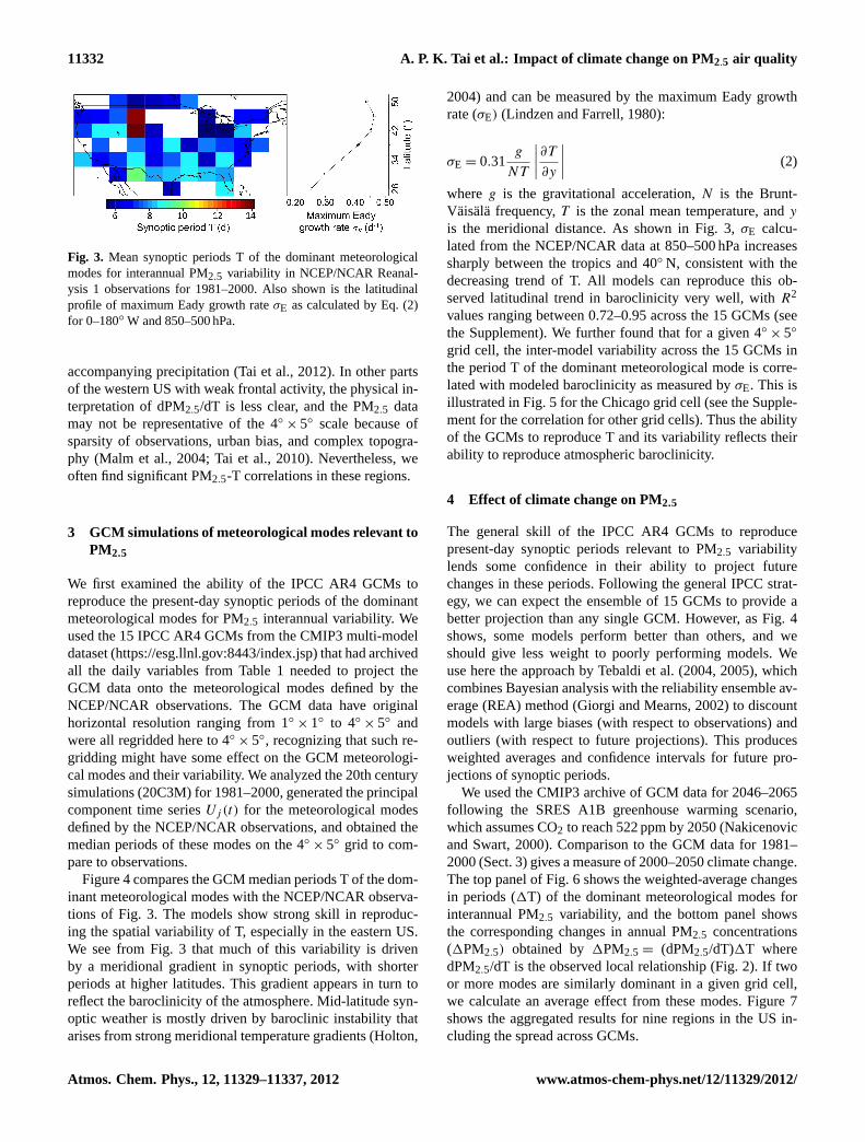
Fig. 3. Mean synoptic periods T of the dominant meteorologicalmodes for interannual PM2.5 variability in NCEP/NCAR Reanal-ysis 1 observations for 1981–2000. Also shown is the latitudinalprofile of maximum Eady growth rateσE as calculated by Eq. (2)for 0–180◦ W and 850–500 hPa.

accompanying precipitation (Tai et al., 2012). In other partsof the western US with weak frontal activity, the physical in-terpretation of dPM2.5/dT is less clear, and the PM2.5 datamay not be representative of the 4◦

× 5◦ scale because ofsparsity of observations, urban bias, and complex topogra-phy (Malm et al., 2004; Tai et al., 2010). Nevertheless, weoften find significant PM2.5-T correlations in these regions.

3 GCM simulations of meteorological modes relevant toPM2.5

We first examined the ability of the IPCC AR4 GCMs toreproduce the present-day synoptic periods of the dominantmeteorological modes for PM2.5 interannual variability. Weused the 15 IPCC AR4 GCMs from the CMIP3 multi-modeldataset (https://esg.llnl.gov:8443/index.jsp) that had archivedall the daily variables from Table 1 needed to project theGCM data onto the meteorological modes defined by theNCEP/NCAR observations. The GCM data have originalhorizontal resolution ranging from 1◦

× 1◦ to 4◦× 5◦ and

were all regridded here to 4◦× 5◦, recognizing that such re-

gridding might have some effect on the GCM meteorologi-cal modes and their variability. We analyzed the 20th centurysimulations (20C3M) for 1981–2000, generated the principalcomponent time seriesUj (t) for the meteorological modesdefined by the NCEP/NCAR observations, and obtained themedian periods of these modes on the 4◦

× 5◦ grid to com-pare to observations.

Figure 4 compares the GCM median periods T of the dom-inant meteorological modes with the NCEP/NCAR observa-tions of Fig. 3. The models show strong skill in reproduc-ing the spatial variability of T, especially in the eastern US.We see from Fig. 3 that much of this variability is drivenby a meridional gradient in synoptic periods, with shorterperiods at higher latitudes. This gradient appears in turn toreflect the baroclinicity of the atmosphere. Mid-latitude syn-optic weather is mostly driven by baroclinic instability thatarises from strong meridional temperature gradients (Holton,

2004) and can be measured by the maximum Eady growthrate (σE) (Lindzen and Farrell, 1980):

σE = 0.31g

NT

∣∣∣∣∂T

∂y

∣∣∣∣ (2)

whereg is the gravitational acceleration,N is the Brunt-Vaisala frequency,T is the zonal mean temperature, andy

is the meridional distance. As shown in Fig. 3,σE calcu-lated from the NCEP/NCAR data at 850–500 hPa increasessharply between the tropics and 40◦ N, consistent with thedecreasing trend of T. All models can reproduce this ob-served latitudinal trend in baroclinicity very well, withR2

values ranging between 0.72–0.95 across the 15 GCMs (seethe Supplement). We further found that for a given 4◦

× 5◦

grid cell, the inter-model variability across the 15 GCMs inthe period T of the dominant meteorological mode is corre-lated with modeled baroclinicity as measured byσE. This isillustrated in Fig. 5 for the Chicago grid cell (see the Supple-ment for the correlation for other grid cells). Thus the abilityof the GCMs to reproduce T and its variability reflects theirability to reproduce atmospheric baroclinicity.

4 Effect of climate change on PM2.5

The general skill of the IPCC AR4 GCMs to reproducepresent-day synoptic periods relevant to PM2.5 variabilitylends some confidence in their ability to project futurechanges in these periods. Following the general IPCC strat-egy, we can expect the ensemble of 15 GCMs to provide abetter projection than any single GCM. However, as Fig. 4shows, some models perform better than others, and weshould give less weight to poorly performing models. Weuse here the approach by Tebaldi et al. (2004, 2005), whichcombines Bayesian analysis with the reliability ensemble av-erage (REA) method (Giorgi and Mearns, 2002) to discountmodels with large biases (with respect to observations) andoutliers (with respect to future projections). This producesweighted averages and confidence intervals for future pro-jections of synoptic periods.

We used the CMIP3 archive of GCM data for 2046–2065following the SRES A1B greenhouse warming scenario,which assumes CO2 to reach 522 ppm by 2050 (Nakicenovicand Swart, 2000). Comparison to the GCM data for 1981–2000 (Sect. 3) gives a measure of 2000–2050 climate change.The top panel of Fig. 6 shows the weighted-average changesin periods (1T) of the dominant meteorological modes forinterannual PM2.5 variability, and the bottom panel showsthe corresponding changes in annual PM2.5 concentrations(1PM2.5) obtained by1PM2.5 = (dPM2.5/dT)1T wheredPM2.5/dT is the observed local relationship (Fig. 2). If twoor more modes are similarly dominant in a given grid cell,we calculate an average effect from these modes. Figure 7shows the aggregated results for nine regions in the US in-cluding the spread across GCMs.

Atmos. Chem. Phys., 12, 11329–11337, 2012 www.atmos-chem-phys.net/12/11329/2012/

A. P. K. Tai et al.: Impact of climate change on PM2.5 air quality 11333

Fig. 4. Scatterplots of modeled vs. observed synoptic periods T of the dominant meteorological modes for interannual PM2.5 variability inthe US for 1981–2000. Observed values are from NCEP/NCAR Reanalysis 1, and modeled values are from 15 IPCC AR4 GCMs. GCMnames are given in each panel, and the symbol above each name is used to identify the model in Figs. 5 and 7. Each data point represents Tfor one 4◦ × 5◦ grid cell, and the ensemble of points represents the continental US separated as eastern (east of 95◦ W), central (110–95◦ W),and western (west of 110◦ W). The solid black line is the reduced major-axis regression slope, with coefficient of variation (R2) also given.The 1: 1 line is shown as dashed.

Fig. 5.Relationship between atmospheric baroclinicity and synopticperiod T of the dominant meteorological mode for PM2.5 variabil-ity in the Chicago grid cell as simulated by 15 IPCC AR4 GCMsfor 1981–2000. The observed value from the NCEP/NCAR Reanal-ysis 1 is also indicated. Baroclinicity is measured as the maximumEady growth rateσE for 44–48◦ N and 850–500 hPa. Each symbolrepresents an individual GCM (see Fig. 4). Correlation coefficientand reduced-major-axis regression slope are also shown.

We see from Fig. 6 that the future climate features a gen-eral increase in PM2.5-relevant synoptic periods in the east-ern US, reflecting a more stagnant mid-latitude tropospherewith reduced ventilation by frontal passages. This is a robustresult which follows from reduced baroclinic instability andpoleward shift of storm tracks associated with greenhousewarming (Geng and Sugi, 2003; Mickley et al., 2004; Yin,2005; Lambert and Fyfe, 2006; Murazaki and Hess, 2006;Pinto et al., 2007; Ulbrich et al., 2008). This in turn leads toa likely (74–91 % chance) increase in annual mean PM2.5,with a weighted mean increase of about 0.1 µg m−3 (North-east, Midwest, and Southeast in Fig. 7). In the Northwest(Pacific and Interior NW in Fig. 7), we find a likely (71–83 % chance) decrease in PM2.5 with a weighted mean ofabout−0.3 µg m−3 due to reduced synoptic periods, albeitwith greater inter-model variability than in the eastern US.This reflects more frequent ventilation by maritime inflowsand scavenging by the associated precipitation, and is con-sistent with the general IPCC finding of increasing westerlyflow over the western parts of mid-latitude continents in thefuture climate (Christensen et al., 2007; Meehl et al., 2007).Projections for other parts of the western US are more uncer-tain. As pointed out earlier, the physical meaning of synopticperiods in the West is less clear than in the East, and the skillof GCMs to reproduce present-day synoptic periods is gen-erally lower (Fig. 4).

www.atmos-chem-phys.net/12/11329/2012/ Atmos. Chem. Phys., 12, 11329–11337, 2012

11334 A. P. K. Tai et al.: Impact of climate change on PM2.5 air quality

Fig. 6. Projected 2000–2050 changes in the periods of the dom-inant meteorological modes for PM2.5 variability (top), and im-plied changes in annual mean PM2.5 (bottom). The changes insynoptic periods (1T) are weighted averages from the ensem-ble of IPCC AR4 GCMs calculated using the Bayesian-REA ap-proach of Tebaldi et al. (2004, 2005). The implied changes inPM2.5 (1PM2.5) are calculated as1PM2.5 = (dPM2.5/dT)1Twhere dPM2.5/dT is the local relationship from Fig. 2. When twoor more meteorological modes have similar correlation with annualPM2.5, an average effect from these modes is calculated.

GCM-CTM studies in the literature have reported±0.1–1 µg m−3 changes in annual mean PM2.5 resulting from2000–2050 climate change, with no consistency across stud-ies (Jacob and Winner, 2009). As pointed out in the Intro-duction, such inconsistency is to be expected since individ-ual studies used a single future-climate realization from asingle GCM. Our multi-model ensemble analysis allows usto conclude with greater confidence that changes in synop-tic circulation brought about by climate change will degradePM2.5 air quality in the eastern US but that the effect will besmall (∼ 0.1 µg m−3). Effects in the western US are poten-tially larger but of uncertain sign even when the ensemble ofIPCC GCMs is considered.

Figure 8 summarizes the projected effects of 2000–2050climate change on annual PM2.5 in the US, drawing fromthis work for circulation changes (including modulation ofprecipitation frequency) and from previous studies for otherclimatic factors. Tai et al. (2012) pointed out that increasingmean temperature, independently from changes in circula-tion, could have a large effect on PM2.5 in the Southeast andsome parts of the western US through changes in emissions,wildfires, and nitrate aerosol volatility. Temperature-drivenchanges in the Southeast may reduce ammonium nitrate by∼ 0.2 µg m−3 due to increased volatility (Tagaris et al., 2007;Pye et al., 2009), but increase organic PM by∼ 0.4 µg m−3

due to increased biogenic emissions (Heald et al., 2008).

Fig. 7. 2000–2050 regional changes in annual mean PM2.5(1PM2.5) due to changes in the periods of dominant meteorologi-cal modes for nine US regions. Regional division follows that of Taiet al. (2012). Symbols represent individual IPCC AR4 GCMs (seeFig. 4). Weighted averages and confidence intervals are calculatedusing the Bayesian-REA approach from Tebaldi et al. (2004, 2005).

Fig. 8. Summary of projected effects of 2000–2050 climate changeon annual PM2.5 in the US as driven by changes in circulation,temperature (biogenic emissions and PM volatility), vegetation dy-namics, and wildfires. The affected regions and PM2.5 componentsare identified (OC≡ organic carbon; BC≡ black carbon). Errorbars represent either the approximate range or standard deviation ofthe estimate. Estimates are from this work (circulation); Tagaris etal. (2007), Heald et al. (2008) and Pye et al. (2009) (temperature);Wu et al. (2012) (vegetation); Spracklen et al. (2009) and Yue etal. (2012) (wildfires). All studies used the IPCC SRES A1B sce-nario for 2000–2050 climate forcing.

Wu et al. (2012) projected a 0.1–0.2 µg m−3 increase in or-ganic PM in the Midwest and western US due to climate-driven changes in ecosystem type. Spracklen et al. (2009)and Yue et al. (2012) projected a∼ 1 µg m−3 increase in sum-mertime carbonaceous aerosols in the Northwest due to in-creased wildfire activities. Tagaris et al. (2007) and Aviseet al. (2009) predicted an average decrease of summertimePM2.5 by ∼ 10 % and∼ 1 µg m−3 by 2050, respectively,

Atmos. Chem. Phys., 12, 11329–11337, 2012 www.atmos-chem-phys.net/12/11329/2012/

A. P. K. Tai et al.: Impact of climate change on PM2.5 air quality 11335

caused primarily by higher precipitation in their GCMs, buttrends in precipitation in most of the US are highly uncertain(Christensen et al., 2007). All in all, none of these effects(or their ensemble) is likely to affect annual mean PM2.5 bymore than 0.5 µg m−3 (∼ 3 % of the current annual standardof 15 µg m−3). Therefore, for PM2.5 regulatory purpose onan annual mean basis, 2000–2050 climate change will rep-resent only a modest penalty or benefit for air quality man-agers toward the achievement of PM2.5 air quality goals. Ofpotentially greater concern would be the effect of increasedwildfires on daily PM2.5 in the western US (Spracklen et al.,2009).

5 Conclusions

PM2.5 air quality depends on a number of regional meteoro-logical variables that are difficult to simulate in general circu-lation models (GCMs). This makes projections of the effectof 21st-century climate change on PM2.5 problematic. Con-sideration of a large ensemble of future-climate simulationsusing a number of independent GCMs can help to reducethe uncertainty. However, this is not computationally prac-tical in the standard GCM-CTM studies where a chemicaltransport model (CTM) is coupled to the GCM for explicitsimulation of air quality. We presented here an alternativemethod by first using climatological observations to identifythe dominant meteorological modes driving PM2.5 variabil-ity, and then analyzing CMIP3 archived data from 15 GCMsto diagnose the effect of 2000–2050 climate change on theperiods of these modes.

We focused on projections of annual mean PM2.5 over a4◦

× 5◦ grid covering the contiguous US. We showed that theobserved 1999–2010 interannual variability of PM2.5 acrossthe US is strongly correlated with the periods (T) of thedominant synoptic-scale meteorological modes, particularlyin the eastern US where these modes correspond to frontalpassages. The observed local relationship dPM2.5/dT thenprovides a means to infer changes in PM2.5 from GCM-simulated changes in T. We find that all GCMs have signif-icant skill in reproducing T and its spatial distribution overthe US, reflecting their ability to capture the baroclinicity ofthe atmosphere. Inter-model differences in synoptic periodscan be largely explained by differences in baroclinicity.

We then examined the 2000–2050 trends in synoptic pe-riods T across the continental US as simulated by the en-semble of GCMs for the SRES A1B greenhouse warmingscenario. We find a general slowing down of synoptic cir-culation in the eastern US, as measured by an increase in T.We infer that changes in circulation driven by climate changewill likely increase annual mean PM2.5 in the eastern US by∼ 0.1 µg m−3, reflecting a more stagnant mid-latitude tropo-sphere and less frequent ventilation by frontal passages. Wealso project a likely decrease by∼ 0.3 µg m−3 in the North-west due to more frequent ventilation by maritime inflows.

Potentially larger regional effects of climate change on PM2.5air quality may arise from changes in temperature, biogenicemissions, wildfires, and vegetation. Overall, however, it isunlikely that 2000–2050 climate change will modify annualmean PM2.5 by more than 0.5 µg m−3. These climate changeeffects, independent of changes in anthropogenic emissions,represent a relatively minor penalty or benefit for PM2.5 reg-ulatory purposes. Of more potential concern would be theeffect of increased wildfires on daily PM2.5.

An important caveat in our approach is the assumptionthat the dPM2.5/dT will remain unchanged and that the samemeteorological modes will remain dominant for PM2.5 vari-ability in the future climate. Very large changes in emissionscould affect the validity of these assumptions. This could beexplored in future work using GCM-CTM studies with per-turbed emissions.

Supplementary material related to this article isavailable online at:http://www.atmos-chem-phys.net/12/11329/2012/acp-12-11329-2012-supplement.pdf.

Acknowledgements.This work was supported by a Mustard SeedFoundation Harvey Fellowship to Amos P. K. ai, and the NASAApplied Sciences Program through the NASA Air Quality AppliedSciences Team (AQAST). We acknowledge the modeling groups,the Program for Climate Model Diagnosis and Intercomparison(PCMDI) and the WCRP’s Working Group on Coupled Modelling(WGCM) for their roles in making available the WCRP CMIP3multi-model dataset. Support of this dataset is provided by theOffice of Science, US Department of Energy. We also thank Su-san C. Anenberg and Carey Jang from US EPA for their thoughtfulinputs and suggestions.

Edited by: C. H. Song

References

Avise, J., Chen, J., Lamb, B., Wiedinmyer, C., Guenther, A.,Salathe, E., and Mass, C.: Attribution of projected changesin summertime US ozone and PM2.5 concentrations to globalchanges, Atmos. Chem. Phys., 9, 1111–1124,doi:10.5194/acp-9-1111-2009, 2009.

Bengtsson, L., Hodges, K. I., and Roeckner, E.: Storm tracks andclimate change, J. Climate, 19, 3518–3543, 2006.

Christensen, J. H., Hewitson, B., Busuioc, A., Chen, A., Gao, X.,Held, I., Jones, R., Kolli, R. K., Kwon, W.-T., Laprise, R., Mag-ana Rueda, V., Mearns, L., Menendez, C. G., Raisanen, J., Rinke,A., Sarr, A., and Whetton, P.: Regional climate projections, in:Climate change 2007: The physical science basis. Contributionof Working Groupi to the Fourth Assessment Report of the In-tergovernmental Panel on Climate Change, Cambridge Univer-sity Press, New York, NY, USA, 847–940, 2007.

Cooper, O. R., Moody, J. L., Parrish, D. D., Trainer, M., Ryerson, T.B., Holloway, J. S., Hubler, G., Fehsenfeld, F. C., Oltmans, S. J.,

www.atmos-chem-phys.net/12/11329/2012/ Atmos. Chem. Phys., 12, 11329–11337, 2012

11336 A. P. K. Tai et al.: Impact of climate change on PM2.5 air quality

and Evans, M. J.: Trace gas signatures of the airstreams withinNorth Atlantic Cyclones: case studies from the North Atlanticregional experiment (NARE ’97) aircraft intensive, J. Geophys.Res.-Atmos., 106, 5437–5456, 2001.

Dawson, J. P., Adams, P. J., and Pandis, S. N.: Sensitivity ofPM2.5 to climate in the Eastern US: a modeling case study, At-mos. Chem. Phys., 7, 4295–4309,doi:10.5194/acp-7-4295-2007,2007.

EPA: Our nation’s air: Status and trends through 2010, U.S. EPAOffice of Air Quality Planning and Standards, Research TrianglePark, NC, 2012.

Geng, Q. Z. and Sugi, M.: Possible change of extratropical cycloneactivity due to enhanced greenhouse gases and sulfate aerosols –study with a high-resolution AGCM, J. Climate, 16, 2262–2274,2003.

Giorgi, F. and Mearns, L. O.: Calculation of average, uncer-tainty range, and reliability of regional climate changes fromAOGCM simulations via the “reliability ensemble averaging”(REA) method, J. Climate, 15, 1141–1158, 2002.

Heald, C. L., Henze, D. K., Horowitz, L. W., Feddema, J., Lamar-que, J. F., Guenther, A., Hess, P. G., Vitt, F., Seinfeld, J. H.,Goldstein, A. H., and Fung, I.: Predicted change in global sec-ondary organic aerosol concentrations in response to future cli-mate, emissions, and land use change, J. Geophys. Res.-Atmos.,113, D05211,doi:10.1029/2007jd009092, 2008.

Holton, J. R.: An introduction to dynamic meteorology, 4th ed.,International geophysics series, 88, Elsevier Academic Press,Burlington, MA, xii, 535 pp., 2004.

Jacob, D. J. and Winner, D. A.: Effect of climate change on air qual-ity, Atmos. Environ., 43, 51–63, 2009.

Kalnay, E., Kanamitsu, M., Kistler, R., Collins, W., Deaven, D.,Gandin, L., Iredell, M., Saha, S., White, G., Woollen, J., Zhu, Y.,Chelliah, M., Ebisuzaki, W., Higgins, W., Janowiak, J., Mo, K.C., Ropelewski, C., Wang, J., Leetmaa, A., Reynolds, R., Jenne,R., and Joseph, D.: The NCEP/NCAR 40-year reanalysis project,B. Am. Meteorol. Soc., 77, 437–471, 1996.

Kistler, R., Kalnay, E., Collins, W., Saha, S., White, G., Woollen,J., Chelliah, M., Ebisuzaki, W., Kanamitsu, M., Kousky, V., vanden Dool, H., Jenne, R., and Fiorino, M.: The NCEP-NCAR 50-year reanalysis: Monthly means CD-ROM and documentation,B. Am. Meteorol. Soc., 82, 247–267, 2001.

Kleeman, M. J.: A preliminary assessment of the sensitivity ofair quality in California to global change, Climatic Change, 87,S273–S292,doi:10.1007/S10584-007-9351-3, 2008.

Lambert, S. J. and Fyfe, J. C.: Changes in winter cyclone frequen-cies and strengths simulated in enhanced greenhouse warmingexperiments: Results from the models participating in the IPCCdiagnostic exercise, Clim. Dynam., 26, 713–728, 2006.

Lang, C. and Waugh, D. W.: Impact of climate change on the fre-quency of Northern Hemisphere summer cyclones, J. Geophys.Res.-Atmos., 116, D04103,doi:10.1029/2010JD014300, 2011.

Li, Q. B., Jacob, D. J., Park, R., Wang, Y. X., Heald, C. L., Hudman,R., Yantosca, R. M., Martin, R. V., and Evans, M.: North Ameri-can pollution outflow and the trapping of convectively lifted pol-lution by upper-level anticyclone, J. Geophys. Res.-Atmos., 110,D10301,doi:10.1029/2004jd005039, 2005.

Liao, H., Chen, W. T., and Seinfeld, J. H.: Role of cli-mate change in global predictions of future troposphericozone and aerosols, J. Geophys. Res.-Atmos., 111, D12304,

doi:10.1029/2005jd006852, 2006.Lindzen, R. S. and Farrell, B.: A simple approximate result for the

maximum growth-rate of baroclinic instabilities, J.Atmos. Sci.,37, 1648–1654, 1980.

Malm, W. C., Schichtel, B. A., Pitchford, M. L., Ashbaugh, L. L.,and Eldred, R. A.: Spatial and monthly trends in speciated fineparticle concentration in the United States, J. Geophys. Res.-Atmos., 109, D03306,doi:10.1029/2003jd003739, 2004.

Meehl, G. A., Stocker, T. F., Collins, W. D., Friedlingstein, P., Gaye,A. T., Gregory, J. M., Kitoh, A., Knutti, R., Murphy, J. M., Noda,A., Raper, S. C. B., Watterson, I. G., Weaver, A. J., and Zhao,Z.-C.: Global climate projections, in: Climate change 2007: Thephysical science basis. Contribution of Working Group I to theFourth Assessment Report of the Intergovernmental Panel onClimate Change, Cambridge University Press, Cambridge, UKand New York, NY, USA, 2007.

Mickley, L. J., Jacob, D. J., Field, B. D., and Rind, D.:Effects of future climate change on regional air pollutionepisodes in the United States, Geophys. Res. Lett., 31, L24103,doi:10.1029/2004gl021216, 2004.

Murazaki, K. and Hess, P.: How does climate change contribute tosurface ozone change over the United States?, J. Geophys. Res.-Atmos., 111, D05301,doi:10.1029/2005jd005873, 2006.

Nakicenovic, N. and Swart, R.: Special report on emissions scenar-ios: A special report of Working Group III of the Intergovern-mental Panel on Climate Change, Cambridge University Press,Cambridge, New York, 599 pp., 2000.

Park, R. J., Jacob, D. J., and Logan, J. A.: Fire and biofuel contribu-tions to annual mean aerosol mass concentrations in the UnitedStates, Atmos. Environ., 41, 7389–7400, 2007.

Pinto, J. G., Ulbrich, U., Leckebusch, G. C., Spangehl, T., Reyers,M., and Zacharias, S.: Changes in storm track and cyclone activ-ity in three sres ensemble experiments with the ECHAM5/MPI-OM1 GCM, Clim. Dynam., 29, 195–210, 2007.

Pye, H. O. T., Liao, H., Wu, S., Mickley, L. J., Jacob, D. J.,Henze, D. K., and Seinfeld, J. H.: Effect of changes in climateand emissions on future sulfate-nitrate-ammonium aerosol lev-els in the United States, J. Geophys. Res.-Atmos., 114, D01205,doi:10.1029/2008jd010701, 2009.

Rind, D., Lerner, J., Jonas, J., and McLinden, C.: Effectsof resolution and model physics on tracer transports inthe NASA Goddard Institute for Space Studies general cir-culation models, J. Geophys. Res.-Atmos., 112, D09315,doi:10.1029/2006jd007476, 2007.

Spracklen, D. V., Mickley, L. J., Logan, J. A., Hudman, R. C.,Yevich, R., Flannigan, M. D., and Westerling, A. L.: Im-pacts of climate change from 2000 to 2050 on wildfire ac-tivity and carbonaceous aerosol concentrations in the west-ern United States, J. Geophys. Res.-Atmos., 114, D20301,doi:10.1029/2008jd010966, 2009.

Tagaris, E., Manomaiphiboon, K., Liao, K. J., Leung, L. R., Woo,J. H., He, S., Amar, P., and Russell, A. G.: Impacts of globalclimate change and emissions on regional ozone and fine partic-ulate matter concentrations over the United States, J. Geophys.Res.-Atmos., 112, D14312,doi:10.1029/2006jd008262, 2007.

Tai, A. P. K., Mickley, L. J., and Jacob, D. J.: Correlations betweenfine particulate matter (PM2.5) and meteorological variables inthe United States: Implications for the sensitivity of PM2.5 toclimate change, Atmos. Environ., 44, 3976–3984, 2010.

Atmos. Chem. Phys., 12, 11329–11337, 2012 www.atmos-chem-phys.net/12/11329/2012/

A. P. K. Tai et al.: Impact of climate change on PM2.5 air quality 11337

Tai, A. P. K., Mickley, L. J., Jacob, D. J., Leibensperger, E. M.,Zhang, L., Fisher, J. A., and Pye, H. O. T.: Meteorological modesof variability for fine particulate matter (PM2.5) air quality inthe United States: implications for PM2.5 sensitivity to climatechange, Atmos. Chem. Phys., 12, 3131–3145,doi:10.5194/acp-12-3131-2012, 2012.

Tebaldi, C., Mearns, L. O., Nychka, D., and Smith, R. L.: Re-gional probabilities of precipitation change: A Bayesian analy-sis of multimodel simulations, Geophys. Res. Lett., 31, L24213,doi:10.1029/2004gl021276, 2004.

Tebaldi, C., Smith, R. L., Nychka, D., and Mearns, L. O.: Quan-tifying uncertainty in projections of regional climate change: ABayesian approach to the analysis of multimodel ensembles, J.Climate, 18, 1524–1540, 2005.

Thishan Dharshana, K. G., Kravtsov, S., and Kahl, J. D. W.: Rela-tionship between synoptic weather disturbances and particulatematter air pollution over the United States, J. Geophys. Res.-Atmos., 115, D24219,doi:10.1029/2010jd014852, 2010.

Ulbrich, U., Pinto, J. G., Kupfer, H., Leckebusch, G. C., Spangehl,T., and Reyers, M.: Changing Northern Hemisphere storm tracksin an ensemble of IPCC climate change simulations, J. Climate,21, 1669–1679,doi:10.1175/2007jcli1992.1, 2008.

Ulbrich, U., Leckebusch, G. C., and Pinto, J. G.: Extra-tropical cy-clones in the present and future climate: A review, Theor. Appl.Climatol., 96, 117–131, 2009.

Wilks, D. S.: Statistical methods in the atmospheric sciences,3rd ed., International geophysics series, 100, Elsevier/AcademicPress, Amsterdam, Boston, xix, 676 pp., 2011.

Wu, S., Mickley, L. J., Kaplan, J. O., and Jacob, D. J.: Impacts ofchanges in land use and land cover on atmospheric chemistryand air quality over the 21st century, Atmos. Chem. Phys., 12,1597–1609,doi:10.5194/acp-12-1597-2012, 2012.

Yin, J. H.: A consistent poleward shift of the storm tracks in simu-lations of 21st century climate, Geophys. Res. Lett., 32, L18701,doi:10.1029/2005gl023684, 2005.

Yue, X., Mickley, L. J., Logan, J. A., and Kaplan, J. O.: Ensembleprojections of wildfire activity and carbonaceous aerosol concen-trations over the western United States in the mid-21st century,in preparation, 2012.

www.atmos-chem-phys.net/12/11329/2012/ Atmos. Chem. Phys., 12, 11329–11337, 2012