impact command reference manual - isp.ncifcrf.govthis is the impact command reference manual. it...
TRANSCRIPT
Impact Command Reference ManualImpact: Integrated Modeling Program using Applied Chemical Theory
Version 5.5, May 2009
For inquiries about Impact
Schrodinger101 SW Main St., Suite 1300Portland, OR 97204503–299–1150503–299–4532 faxEmail: [email protected]
Copyright c© 2009 Schrodinger, LLC All rights reserved.
CombiGlide, Epik, Glide, Impact, Jaguar, Liaison, LigPrep, Mae-stro, Phase, Prime, QikProp, QikFit, QikSim, QSite, SiteMap, andStrike are trademarks of Schrodinger, LLC. Schrodinger and Macro-Model are registered trademarks of Schrodinger, LLC.The C and C++ libraries for parsing PDB records are a copyrightedwork (1989) of the Regents of the University of California. Allrights reserved.To the maximum extent permitted by applicable law, this pub-lication is provided “as is” without warranty of any kind. Thispublication may contain trademarks of other companies.Please note that any third party programs (“Third Party Pro-grams”) or third party Web sites (“Linked Sites”) referred to inthis document may be subject to third party license agreementsand fees. Schrodinger, LLC and its affiliates have no responsibilityor liability, directly or indirectly, for the Third Party Programs orfor the Linked Sites or for any damage or loss alleged to be causedby or in connection with use of or reliance thereon. Any warrantiesthat we make regarding our own products and services do not applyto the Third Party Programs or Linked Sites, or to the interactionbetween, or interoperability of, our products and services and theThird Party Programs. Referrals and links to Third Party Pro-grams and Linked Sites do not constitute an endorsement of suchThird Party Programs or Linked Sites.
Impact Version 55108May 2009
Chapter 1: Introduction to Impact
1 Introduction to Impact
ImpactTM (Integrated Modeling Program using Applied Chemical Theory) isan integrated program for molecular mechanics simulations.1 It allows theuser to define the simulation system (usually a protein or DNA molecule inaqueous solution) and to perform Monte Carlo or molecular dynamics sim-ulations. In addition, the user has at her/his disposal a whole array of toolsfor analyzing the results of the simulations. Finally, Impact is the “driver”for the high-throughput ligand screening program GlideTM, the LiaisonTM
module for calculating ligand binding energies, and the mixed mode Quan-tum Mechanics/Molecular Mechanics program QSiteTM.This is the Impact Command Reference Manual. It documents using Impactfrom the command-line, and all the keywords of Impact input files. RunningImpact from Maestro, and discussion of the principal applications Glide,Liaison, and QSite, are more fully documented in other manuals:• Glide Quick Start Guide
A collection of tutorial examples that illustrate the use of Glide.• Glide User Manual
A description of Glide, focusing on its use from Maestro.• Glide Technical Notes
A collection of case studies elaborating on the scientific methods andresults of Glide.
• Liaison User Manual
A description of Liaison, including its use from Maestro, a tutorial, andnotes on the scientific methods and results.
• QSite User Manual
A description of QSite, including its use from Maestro, a tutorial, andnotes on the scientific methods and results.
1.1 A Brief History of ImpactThe current commercial version of Impact and the Glide, Liaison, and QSiteproducts was developed from the academic Impact originally designed in thelaboratory of Professor Ronald M. Levy at Rutgers University. The followingpeople have contributed to the development of Impact:
1.1.1 Commercial Versions
• v5.0 (June 2008) Jay Banks, Yixiang Cao, Wolfgang Damm, RichardFriesner, Emilio Gallicchio, Thomas Halgren, Ronald Levy, DanielMainz, Rob Murphy, and Matt Repasky
1 J. L. Banks et al., J. Comp. Chem., 26, 1752-1780 (2005)
Impact 5.5 Command Reference Manual 1
Chapter 1: Introduction to Impact
• v4.0 (November 2005) Jay Banks, Yixiang Cao, Wolfgang Damm,Richard Friesner, Emilio Gallicchio, Thomas Halgren, Ronald Levy,Daniel Mainz, Rob Murphy, Matt Repasky, and Linda Zhang.
• v3.5 (January 2005) Jay Banks, Yixiang Cao, Wolfgang Damm, RichardFriesner, Emilio Gallicchio, Thomas Halgren, Ronald Levy, DanielMainz, Rob Murphy, Matt Repasky, and Linda Zhang.
• v3.0 (June 2004) Jay Banks, Yixiang Cao, Wolfgang Damm, RichardFriesner, Emilio Gallicchio, Thomas Halgren, Ronald Levy, DanielMainz, Rob Murphy, and Matt Repasky.
• v2.7 (October 2003) Jay Banks, Yixiang Cao, Wolfgang Damm, RichardFriesner, Emilio Gallicchio, Thomas Halgren, Ronald Levy, DanielMainz, Rob Murphy, and Matt Repasky.
• v2.5 (January 2003) Jay Banks, Yixiang Cao, Wolfgang Damm, RichardFriesner, Emilio Gallicchio, Thomas Halgren, Ronald Levy, DanielMainz, and Rob Murphy.
• v2.0 (June 2002). Jay Banks, Yixiang Cao, Wolfgang Damm, RichardFriesner, Emilio Gallicchio, Thomas Halgren, Ronald Levy, DanielMainz, and Rob Murphy.
• v1.8 (September 2001). Jay Banks, Yixiang Cao, Wolfgang Damm,Richard Friesner, Emilio Gallicchio, Thomas Halgren, Ronald Levy,Daniel Mainz, and Rob Murphy.
• v1.7 (March 2001). Jay Banks, Yixiang Cao, Richard Friesner, EmilioGallicchio, Thomas Halgren, Ronald Levy, Daniel Mainz, Rob Murphy,and Ruhong Zhou.
• v1.6 (November 2000). Jay Banks, Michael Beachy, Yixiang Cao,Richard Friesner, Emilio Gallicchio, Ronald Levy, Daniel Mainz, RobMurphy, and Ruhong Zhou.
• v1.0 (June 1999). Jay Banks, Richard Friesner, Emilio Gallicchio, Avi-jit Ghosh, Ronald Levy, Rob Murphy, Anders Wallqvist, and RuhongZhou.
• v0.95 (Nov 1998). Jay Banks, Richard Friesner, Emilio Gallicchio, Avi-jit Ghosh, Ronald Levy, Rob Murphy, Anders Wallqvist, and RuhongZhou.
• v0.9 (Aug 1998). Jay Banks, Mark Friedrichs, Richard Friesner, EmilioGallicchio, Avijit Ghosh, Ronald Levy, Rob Murphy, Anders Wallqvist,and Ruhong Zhou.
• v0.8 (May 1998). Jay Banks, Chris Cortis, Shlomit Edinger, MarkFriedrichs, Richard Friesner, Emilio Gallicchio, Avijit Ghosh, RonaldLevy, Rob Murphy, Anders Wallqvist, and Ruhong Zhou.
1.1.2 Academic Versions
2 Impact 5.5 Command Reference Manual
Chapter 1: Introduction to Impact
• V7.0 (August 1996). Jay Banks, Yanbo Ding, Gabriela Del Buono,Francisco Figueirido, Ronald Levy, and Ruhong Zhou.
• V6.0 (January 1994). Les Clowney, Francisco Figueirido, Ronald Levy,Lynne Reed, Maureen Smith-Brown, Asif Suri and John Westbrook.
• V5.8 (December 10, 1991). Les Clowney, Francisco Figueirido, DouglasKitchen, Ronald Levy, Maureen Smith, Asif Suri and John Westbrook.
• V5.7 (December 17, 1990). Steve Back, Teresa Head-Gordon, DouglasKitchen, Dorothy Kominos, Ronald Levy and John Westbrook.
• V5.5 and earlier (June 1990). Steve Back, Donna Bassolino, JohnBlair, Fumio Hirata, Douglas Kitchen, David Kofke, Dorothy Kominos,Ronald Levy, Asif Suri and John Westbrook.
1.2 Major FeaturesThe major features of Impact include:• Energy Minimization• Molecular Dynamics• Fast Multipole Method (FMM)• Multiple Time-step Algorithm r-RESPA• S-Walking/J-Walking Methods• Explicit Solvation Model• Poisson-Boltzmann Continuum Solvation (PBF)• Surface Generalized Born Solvation Model (SGB)• OPLS-AA with Automatic Atomtype Recognition• Flexible Schemes for Freezing Part of System• QSite: Mixed-Mode QM/MM Simulations for Reactive Chemistry• Liaison: Calculating and Predicting Ligand Binding Energies• Glide: High-Throughput Ligand-Receptor Docking
1.3 Hardware RequirementsSchrodinger tests and distributes Glide 5.5, Liaison 5.5 and QSite 5.5 forSGI IRIX, IBM AIX, and Intel-x86 compatible Linux-based machines atthis time. Impact 5.5 is not distributed separately from these products. Forcurrent information on other platforms, please contact Schrodinger.
1.4 InstallationTo install Glide, Liaison, or QSite, see the Schrodinger Installation Guide. APDF version of this manual and product documentation should be on yourproduct CD.For those that want to get started quickly, installation is often as easy asrunning:
Impact 5.5 Command Reference Manual 3
Chapter 1: Introduction to Impact
% /bin/sh INSTALL
from the CD, and following the prompts. But please see the InstallationGuide.After installation, in the directory specified by your $SCHRODINGER environ-ment variable, there should be an Impact directory labelled with the currentversion number, at this printing, this is ‘impact-v55108’. In that directory,there are seven subdirectories:
bin/ The executable binary and scripts for running all manner ofImpact-based jobs. Since these are platform-dependent, thesefiles are separated into further subdirectories with their plat-form’s designation, e.g. Linux-x86/.
data/ The database parameters for the AMBER and the OPLS seriesof force fields.
docs/ Electronic versions of the Impact Reference Manual (this docu-ment) are located here.
lib/ Platform-dependent shared libraries needed by Impact are kepthere.
disabled_lib/Disabled shared libraries, moved from the ‘lib/’ subdirectoryshould be kept here. Disabling libraries should only be donewithin Schrodinger’s recommendations.
samples/ The example files noted in this manual’s appendices.
tutorial/Files that correspond to the instructional material in the GlideQuick Start Guide, Liaison User Manual, and QSite User Manualthat walks you through various types of calculations.
A file ‘compatibility’ is also in your ‘impact-v55108’ directory, listing theminimum version numbers of other Schrodinger products compatible withthis Impact release. All Schrodinger startup scripts will use this informationautomatically.The single important environment variable each Impact user has to have is$SCHRODINGER. It should be set to your top-level installation directory forSchrodinger products, e.g. /usr/local/bin/schrodinger. If you plan onusing some of the utility scripts from a command-line interface, you mightlike to add the directory $SCHRODINGER/utilities to your PATH enviromentvariable, so that the scripts in this directory are accessible by name withoutthe full directory name prepended. If your command-line shell is sh, ksh, orbash, this is done by:
(sh/ksh/bash)% export PATH=$PATH:$SCHRODINGER/utilities
and if your shell is csh or tcsh, then do:(csh/tcsh)% setenv PATH $PATH:$SCHRODINGER/utilities
4 Impact 5.5 Command Reference Manual
Chapter 1: Introduction to Impact
To run an Impact example, first make sure that $SCHRODINGER is set to yourSchrodinger installation directory. Then cd to one of example directory andtype:
% $SCHRODINGER/impact -i input_file -o log_file
This will read from the input file and write the log file to log file. If -o isnot specified, Impact will set the log file name to be the same as your inputfile, but with a .log extension in place of .inp.Note that the log file (stdout) is not the file specified in the top writecommand in the input file, which is usually more detailed than the log file.Just typing impact with no arguments is equivalent to typing main1m: theprogram then looks for an input file named ‘fort.1’, and writes to standardoutput.If an input file is specified but a log file is not, Impact constructs the logfile name by appending the suffix .log to the input file name, after firstremoving the suffix .inp if it is present. Thus
% $SCHRODINGER/impact -i myfile
and% $SCHRODINGER/impact -i myfile.inp
will both result in writing a log file called myfile.log.
1.5 Input FilesInstructions for Impact are placed in the main input file, which is then givenas the -i argument to the impact execution script.2 The program executescommands in the input file sequentially, or as directed by control structuresin Impact’s input scripting language, DICE. See Chapter 4 [Advanced InputScripts], page 131, for details of control structures, variables, and advancedfeatures of DICE. Here is a simple example:
WRITE file example.out -
title Example *
CREATE
build primary name species1 type auto read maestro -
file "example.mae"
build types name species1
QUIT
SETMODEL
setpotential
mmechanics consolv agbnp
quit
read parm file paramstd noprint
energy parm cutoff 9.5 listupdate 10 diel 1.0 nodist
energy rescutoff byatom all
2 Historically, the main input file had to be assigned to FORTRAN unit number 1, whichusually as the filename ‘fort.1’. The name may be different on other machines.
Impact 5.5 Command Reference Manual 5
Chapter 1: Introduction to Impact
zonecons auto
QUIT
DYNAMICS
input cntl -
nstep 1000 delt 0.001 stop rotations -
constant totalenergy nprnt 50 tol 1.e-7
run
write maestro file "example_out.mae"
QUIT
END
The input file always begins with a description of where to write the outputgenerated by Impact during its execution, and ends with the keyword endon a single line. The following meta-example is the simplest legal Impactprogram:
write file fname title your_favorite_title *
end
An optional verbose value argument before the * specifies the verbosity ofoutput from various parts of Impact.After the opening write statement, one specifies a sequence of tasks thatImpact should execute. In Impact tasks correspond to a high-level descrip-tion of the computer experiment. For example, the task create sets up theinternal variables describing the molecular structure of the system of inter-est, while inside of task dynamics one runs a molecular dynamics simulation.Typically it is important that tasks are executed in the correct order, whichis usually dictated by common sense (the least common of the senses).3
A task by itself does not produce any side effects. For instance, the fragmentcreate
quit
would do exactly nothing. When Impact begins executing a task it sets up aspecial environment, which is task-dependent. This environment exists untilthe keyword quit is encountered, closing the task. Within each of theseenvironments different collections of commands (subtasks) are in effect. Forinstance, within the create task one can execute the subtask build, but itis not defined inside of the task dynamics. Trying to execute build insideof the latter task would lead to an error.Impact requires that tasks (as well as their matching quit) be declared ona line by themselves. Subtasks, on the other hand, come in several flavors.They must always be the first non-blank word on a line and most often theyare followed on the same line by a series of subtask-specific keywords and
3 For example, few people we know would run a dynamics simulation before setting thesystem up.
6 Impact 5.5 Command Reference Manual
Chapter 1: Introduction to Impact
parameter values. A few, however, have the same formatting requirementsas tasks do, and must be ended by the keyword quit.4
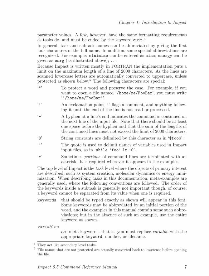
In general, task and subtask names can be abbreviated by giving the firstfour characters of the full name. In addition, some special abbreviations arerecognized. For example: minimize can be entered as minm; energy can begiven as enrg (as illustrated above); . . .Because Impact is written mostly in FORTRAN the implementation puts alimit on the maximum length of a line of 2000 characters. As the lines arescanned lowercase letters are automatically converted to uppercase, unlessprotected as shown below.5 The following characters are special:‘"’ To protect a word and preserve the case. For example, if you
want to open a file named ‘/home/me/FooBar’, you must write‘"/home/me/FooBar"’.
‘!’ An exclamation point ‘!’ flags a comment, and anything follow-ing it until the end of the line is not read or processed.
‘-’ A hyphen at a line’s end indicates the command is continued onthe next line of the input file. Note that there should be at leastone space before the hyphen and that the sum of the lengths ofthe continued lines must not exceed the limit of 2000 characters.
‘$’ String constants are delimited by this character as in ‘$foo$’.‘’’ The quote is used to delimit names of variables used in Impact
input files, as in ‘while ’foo’ lt 10’.‘*’ Sometimes portions of command lines are terminated with an
asterisk. It is required wherever it appears in the examples.The top level of Impact is the task level where the objects of primary interestare described, such as system creation, molecular dynamics or energy mini-mization. When describing tasks in this documentation, meta-examples aregenerally used, where the following conventions are followed. The order ofthe keywords inside a subtask is generally not important though, of course,a keyword cannot be separated from its value when one is required.keywords that should be typed exactly as shown will appear in this font.
Some keywords may be abbreviated by an initial portion of theword, and the examples in this manual contain some such abbre-viations; but in the absence of such an example, use the entirekeyword as shown.
variablesare meta-keywords, that is, you must replace variable with theappropriate keyword, number, or filename.
4 They act like secondary level tasks.5 File names that are not protected are actually converted back to lowercase before opening
the file.
Impact 5.5 Command Reference Manual 7
Chapter 1: Introduction to Impact
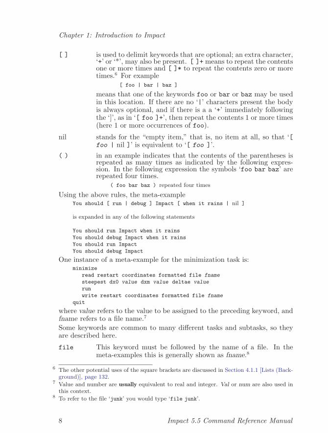
[ ] is used to delimit keywords that are optional; an extra character,‘+’ or ‘*’, may also be present. [ ]+ means to repeat the contentsone or more times and [ ]* to repeat the contents zero or moretimes.6 For example
[ foo | bar | baz ]
means that one of the keywords foo or bar or baz may be usedin this location. If there are no ‘|’ characters present the bodyis always optional, and if there is a a ‘+’ immediately followingthe ‘]’, as in ‘[ foo ]+’, then repeat the contents 1 or more times(here 1 or more occurrences of foo).
nil stands for the “empty item,” that is, no item at all, so that ‘[foo | nil ]’ is equivalent to ‘[ foo ]’.
( ) in an example indicates that the contents of the parentheses isrepeated as many times as indicated by the following expres-sion. In the following expression the symbols ‘foo bar baz’ arerepeated four times.
( foo bar baz ) repeated four times
Using the above rules, the meta-exampleYou should [ run | debug ] Impact [ when it rains | nil ]
is expanded in any of the following statements
You should run Impact when it rains
You should debug Impact when it rains
You should run Impact
You should debug Impact
One instance of a meta-example for the minimization task is:minimize
read restart coordinates formatted file fname
steepest dx0 value dxm value deltae value
run
write restart coordinates formatted file fname
quit
where value refers to the value to be assigned to the preceding keyword, andfname refers to a file name.7
Some keywords are common to many different tasks and subtasks, so theyare described here.
file This keyword must be followed by the name of a file. In themeta-examples this is generally shown as fname.8
6 The other potential uses of the square brackets are discussed in Section 4.1.1 [Lists (Back-ground)], page 132.
7 Value and number are usually equivalent to real and integer. Val or num are also used inthis context.
8 To refer to the file ‘junk’ you would type ‘file junk’.
8 Impact 5.5 Command Reference Manual
Chapter 1: Introduction to Impact
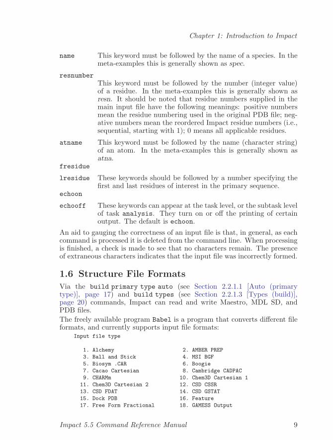
name This keyword must be followed by the name of a species. In themeta-examples this is generally shown as spec.
resnumberThis keyword must be followed by the number (integer value)of a residue. In the meta-examples this is generally shown asresn. It should be noted that residue numbers supplied in themain input file have the following meanings: positive numbersmean the residue numbering used in the original PDB file; neg-ative numbers mean the reordered Impact residue numbers (i.e.,sequential, starting with 1); 0 means all applicable residues.
atname This keyword must be followed by the name (character string)of an atom. In the meta-examples this is generally shown asatna.
fresidue
lresidue These keywords should be followed by a number specifying thefirst and last residues of interest in the primary sequence.
echoon
echooff These keywords can appear at the task level, or the subtask levelof task analysis. They turn on or off the printing of certainoutput. The default is echoon.
An aid to gauging the correctness of an input file is that, in general, as eachcommand is processed it is deleted from the command line. When processingis finished, a check is made to see that no characters remain. The presenceof extraneous characters indicates that the input file was incorrectly formed.
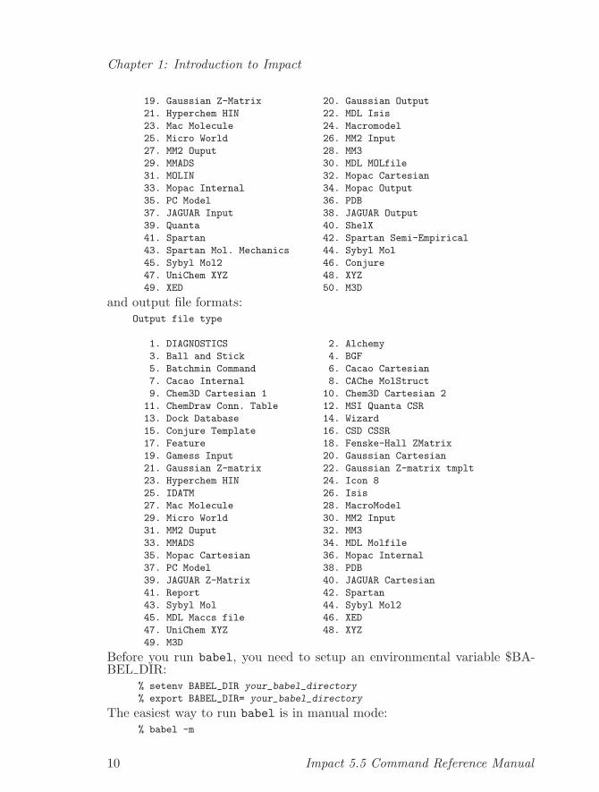
1.6 Structure File FormatsVia the build primary type auto (see Section 2.2.1.1 [Auto (primarytype)], page 17) and build types (see Section 2.2.1.3 [Types (build)],page 20) commands, Impact can read and write Maestro, MDL SD, andPDB files.The freely available program Babel is a program that converts different fileformats, and currently supports input file formats:
Input file type
1. Alchemy 2. AMBER PREP
3. Ball and Stick 4. MSI BGF
5. Biosym .CAR 6. Boogie
7. Cacao Cartesian 8. Cambridge CADPAC
9. CHARMm 10. Chem3D Cartesian 1
11. Chem3D Cartesian 2 12. CSD CSSR
13. CSD FDAT 14. CSD GSTAT
15. Dock PDB 16. Feature
17. Free Form Fractional 18. GAMESS Output
Impact 5.5 Command Reference Manual 9
Chapter 1: Introduction to Impact
19. Gaussian Z-Matrix 20. Gaussian Output
21. Hyperchem HIN 22. MDL Isis
23. Mac Molecule 24. Macromodel
25. Micro World 26. MM2 Input
27. MM2 Ouput 28. MM3
29. MMADS 30. MDL MOLfile
31. MOLIN 32. Mopac Cartesian
33. Mopac Internal 34. Mopac Output
35. PC Model 36. PDB
37. JAGUAR Input 38. JAGUAR Output
39. Quanta 40. ShelX
41. Spartan 42. Spartan Semi-Empirical
43. Spartan Mol. Mechanics 44. Sybyl Mol
45. Sybyl Mol2 46. Conjure
47. UniChem XYZ 48. XYZ
49. XED 50. M3D
and output file formats:Output file type
1. DIAGNOSTICS 2. Alchemy
3. Ball and Stick 4. BGF
5. Batchmin Command 6. Cacao Cartesian
7. Cacao Internal 8. CAChe MolStruct
9. Chem3D Cartesian 1 10. Chem3D Cartesian 2
11. ChemDraw Conn. Table 12. MSI Quanta CSR
13. Dock Database 14. Wizard
15. Conjure Template 16. CSD CSSR
17. Feature 18. Fenske-Hall ZMatrix
19. Gamess Input 20. Gaussian Cartesian
21. Gaussian Z-matrix 22. Gaussian Z-matrix tmplt
23. Hyperchem HIN 24. Icon 8
25. IDATM 26. Isis
27. Mac Molecule 28. MacroModel
29. Micro World 30. MM2 Input
31. MM2 Ouput 32. MM3
33. MMADS 34. MDL Molfile
35. Mopac Cartesian 36. Mopac Internal
37. PC Model 38. PDB
39. JAGUAR Z-Matrix 40. JAGUAR Cartesian
41. Report 42. Spartan
43. Sybyl Mol 44. Sybyl Mol2
45. MDL Maccs file 46. XED
47. UniChem XYZ 48. XYZ
49. M3D
Before you run babel, you need to setup an environmental variable $BA-BEL DIR:
% setenv BABEL_DIR your_babel_directory
% export BABEL_DIR= your_babel_directory
The easiest way to run babel is in manual mode:% babel -m
10 Impact 5.5 Command Reference Manual
Chapter 1: Introduction to Impact
and follow instructions to select desired input and output file formats. Youcan also run babel from the command line, as in
% babel -ix myfile.xyz -renum -oai myfile.dat "AM1 MMOK T=30000"
This will create a MOPAC input file with atom 1 from myfile.xyz as atom1 in myfile.dat. For details of how to run babel, etc, consult the READMEfiles under the babel directory. babel also comes with Schrodinger’s productJaguar, and is accessible therein via the jaguar babel command.
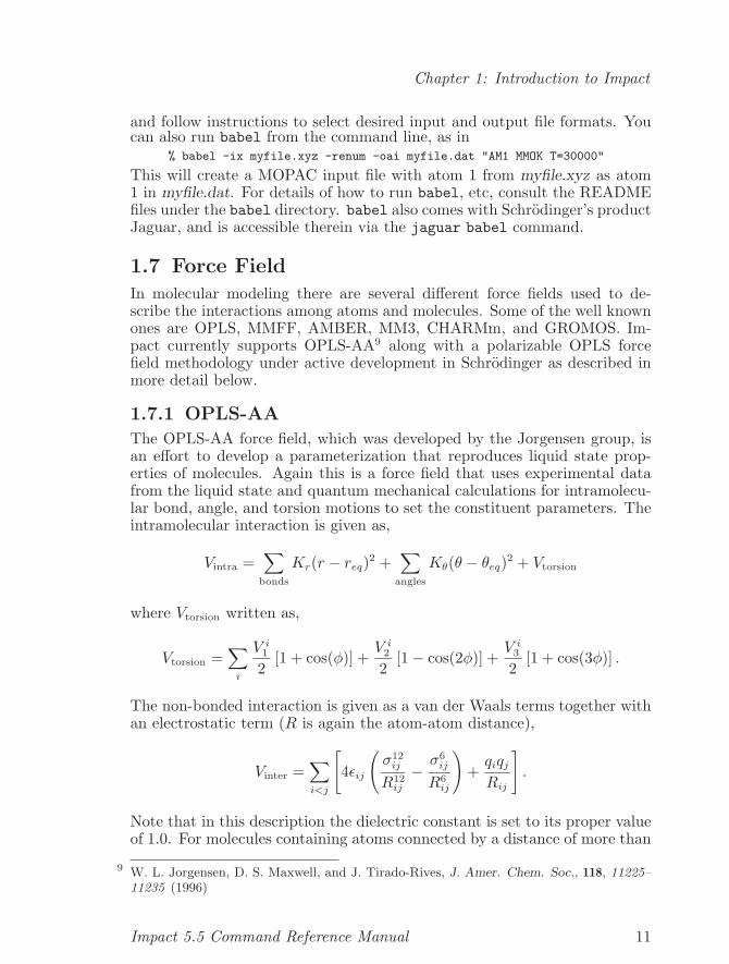
1.7 Force FieldIn molecular modeling there are several different force fields used to de-scribe the interactions among atoms and molecules. Some of the well knownones are OPLS, MMFF, AMBER, MM3, CHARMm, and GROMOS. Im-pact currently supports OPLS-AA9 along with a polarizable OPLS forcefield methodology under active development in Schrodinger as described inmore detail below.
1.7.1 OPLS-AA
The OPLS-AA force field, which was developed by the Jorgensen group, isan effort to develop a parameterization that reproduces liquid state prop-erties of molecules. Again this is a force field that uses experimental datafrom the liquid state and quantum mechanical calculations for intramolecu-lar bond, angle, and torsion motions to set the constituent parameters. Theintramolecular interaction is given as,
Vintra =∑
bonds
Kr(r − req)2 +∑
angles
Kθ(θ − θeq)2 + Vtorsion
where Vtorsion written as,
Vtorsion =∑
i
V i1
2[1 + cos(φ)] +
V i2
2[1− cos(2φ)] +
V i3
2[1 + cos(3φ)] .
The non-bonded interaction is given as a van der Waals terms together withan electrostatic term (R is again the atom-atom distance),
Vinter =∑i<j
[4εij
(σ12
ij
R12ij
−σ6
ij
R6ij
)+qiqj
Rij
].
Note that in this description the dielectric constant is set to its proper valueof 1.0. For molecules containing atoms connected by a distance of more than
9 W. L. Jorgensen, D. S. Maxwell, and J. Tirado-Rives, J. Amer. Chem. Soc., 118, 11225–11235 (1996)
Impact 5.5 Command Reference Manual 11
Chapter 1: Introduction to Impact
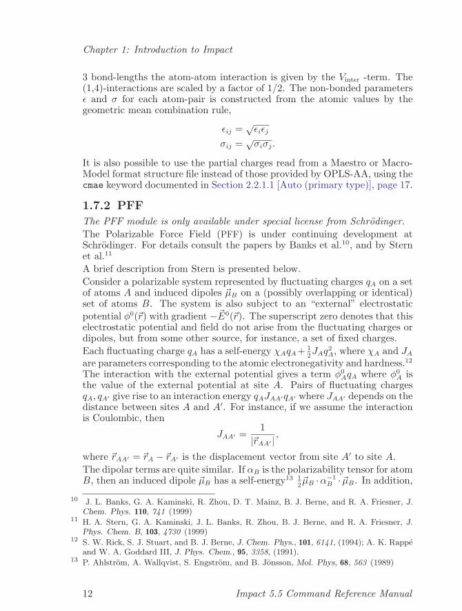
3 bond-lengths the atom-atom interaction is given by the Vinter -term. The(1,4)-interactions are scaled by a factor of 1/2. The non-bonded parametersε and σ for each atom-pair is constructed from the atomic values by thegeometric mean combination rule,
εij =√εiεj
σij =√σiσj.
It is also possible to use the partial charges read from a Maestro or Macro-Model format structure file instead of those provided by OPLS-AA, using thecmae keyword documented in Section 2.2.1.1 [Auto (primary type)], page 17.
1.7.2 PFF
The PFF module is only available under special license from Schrodinger.The Polarizable Force Field (PFF) is under continuing development atSchrodinger. For details consult the papers by Banks et al.10, and by Sternet al.11
A brief description from Stern is presented below.Consider a polarizable system represented by fluctuating charges qA on a setof atoms A and induced dipoles ~µB on a (possibly overlapping or identical)set of atoms B. The system is also subject to an “external” electrostaticpotential φ0(~r) with gradient −~E0(~r). The superscript zero denotes that thiselectrostatic potential and field do not arise from the fluctuating charges ordipoles, but from some other source, for instance, a set of fixed charges.Each fluctuating charge qA has a self-energy χAqA+ 1
2JAq
2A, where χA and JA
are parameters corresponding to the atomic electronegativity and hardness.12The interaction with the external potential gives a term φ0
AqA where φ0A is
the value of the external potential at site A. Pairs of fluctuating chargesqA, qA′ give rise to an interaction energy qAJAA′qA′ where JAA′ depends on thedistance between sites A and A′. For instance, if we assume the interactionis Coulombic, then
JAA′ =1
|~rAA′ |,
where ~rAA′ = ~rA −~rA′ is the displacement vector from site A′ to site A.The dipolar terms are quite similar. If αB is the polarizability tensor for atomB, then an induced dipole ~µB has a self-energy13 1
2~µB ·α−1
B ·~µB. In addition,
10 J. L. Banks, G. A. Kaminski, R. Zhou, D. T. Mainz, B. J. Berne, and R. A. Friesner, J.Chem. Phys. 110, 741 (1999)
11 H. A. Stern, G. A. Kaminski, J. L. Banks, R. Zhou, B. J. Berne, and R. A. Friesner, J.Phys. Chem. B, 103, 4730 (1999)
12 S. W. Rick, S. J. Stuart, and B. J. Berne, J. Chem. Phys., 101, 6141, (1994); A. K. Rappeand W. A. Goddard III, J. Phys. Chem., 95, 3358, (1991).
13 P. Ahlstrom, A. Wallqvist, S. Engstrom, and B. Jonsson, Mol. Phys, 68, 563 (1989)
12 Impact 5.5 Command Reference Manual
Chapter 1: Introduction to Impact
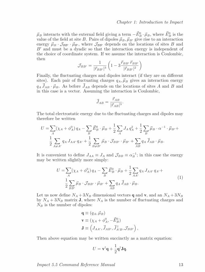
~µB interacts with the external field giving a term −~E0B ·~µB, where ~E0
B is thevalue of the field at site B. Pairs of dipoles ~µB, ~µB′ give rise to an interactionenergy ~µB · JBB′ · ~µB′ , where JBB′ depends on the locations of sites B andB′ and must be a dyadic so that the interaction energy is independent ofthe choice of coordinate system. If we assume the interaction is Coulombic,then
JBB′ =1
|~rBB′ |3(
1− 3~rBB′ ~rBB′
|~rBB′ |2)
Finally, the fluctuating charges and dipoles interact (if they are on differentsites). Each pair of fluctuating charges qA, ~µB gives an interaction energyqA~JAB · ~µB. As before ~JAB depends on the locations of sites A and B and
in this case is a vector. Assuming the interaction is Coulombic,
~JAB =~rAB
|~rAB|3.
The total electrostatic energy due to the fluctuating charges and dipoles maytherefore be written
U =∑A
(χA + φ0A) qA −
∑B
~E0B · ~µB +
12
∑A
JA q2A +
12
∑B
~µB · α−1 · ~µB′+
12
∑A 6=A′
qA JAA′ qA′ +12
∑B 6=B′
~µB · JBB′ · ~µB′ +∑AB
qA~JAB · ~µB.
It is convenient to define JAA ≡ JA and JBB ≡ α−1B ; in this case the energy
may be written slightly more simply:
U =∑A
(χA + φ0A) qA −
∑B
~E0B · ~µB +
12
∑AA′
qA JAA′ qA′+
12
∑BB′
~µB · JBB′ · ~µB′ +∑AB
qA~JAB · ~µB.
(1)
Let us now define NA +3NB dimensional vectors q and v, and an NA +3NB
by NA + 3NB matrix J, where NA is the number of fluctuating charges andNB is the number of dipoles:
q ≡ (qA, ~µB)
v ≡ (χA + φ0A,−~E0
B)
J ≡(JAA′ , ~JAB′ , ~J †
A′B,JBB′
),
Then above equation may be written succinctly as a matrix equation:
U = v†q +12q†Jq.
Impact 5.5 Command Reference Manual 13
Chapter 1: Introduction to Impact
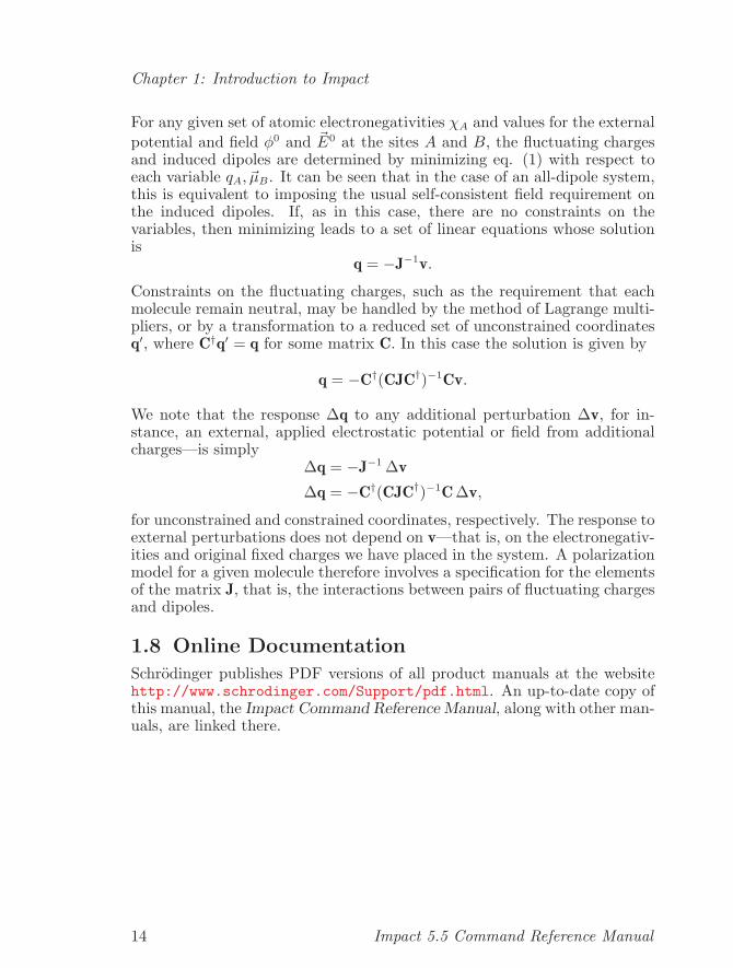
For any given set of atomic electronegativities χA and values for the externalpotential and field φ0 and ~E0 at the sites A and B, the fluctuating chargesand induced dipoles are determined by minimizing eq. (1) with respect toeach variable qA, ~µB. It can be seen that in the case of an all-dipole system,this is equivalent to imposing the usual self-consistent field requirement onthe induced dipoles. If, as in this case, there are no constraints on thevariables, then minimizing leads to a set of linear equations whose solutionis
q = −J−1v.
Constraints on the fluctuating charges, such as the requirement that eachmolecule remain neutral, may be handled by the method of Lagrange multi-pliers, or by a transformation to a reduced set of unconstrained coordinatesq′, where C†q′ = q for some matrix C. In this case the solution is given by
q = −C†(CJC†)−1Cv.
We note that the response ∆q to any additional perturbation ∆v, for in-stance, an external, applied electrostatic potential or field from additionalcharges—is simply
∆q = −J−1 ∆v
∆q = −C†(CJC†)−1C ∆v,
for unconstrained and constrained coordinates, respectively. The response toexternal perturbations does not depend on v—that is, on the electronegativ-ities and original fixed charges we have placed in the system. A polarizationmodel for a given molecule therefore involves a specification for the elementsof the matrix J, that is, the interactions between pairs of fluctuating chargesand dipoles.
1.8 Online DocumentationSchrodinger publishes PDF versions of all product manuals at the websitehttp://www.schrodinger.com/Support/pdf.html. An up-to-date copy ofthis manual, the Impact Command Reference Manual, along with other man-uals, are linked there.
14 Impact 5.5 Command Reference Manual
Chapter 2: Setup System
2 Setup System
This chapter describes tasks to set up Impact simulations: create system,and set up models, etc. This should be done before any real simulation taskscan be performed.
2.1 Set commandsThese commands are not true tasks, in that they are completely specifiedon one line, with no subtasks and no quit keyword. They are used tospecify conditions of the Impact execution that typically remain the samethroughout the duration of the program, so they should usually occur atthe beginning of the input file, either immediately after or even before theinitial write command that specifies the main output file. In particular,set ffield may have unpredictable results if it occurs in the middle of aninput script, or if two or more set ffield commands are issued in the samescript.
2.1.1 Set PathThis command specifies a directory where Impact will look for input filesspecified in subsequent commands. The directory name is added to alist stored in memory. When Impact starts up, the list contains ‘.’(the current working directory), and a default directory that normally is‘$SCHRODINGER/impact-v5.5/data’. The set path command adds one di-rectory to the end of this list. Thus the specified directory will be searchedonly for files that cannot be found in the current working directory, the de-fault directory, or directories specified by previous set path or set ffieldcommands. To specify more than one directory, use more than one set pathcommand, one for each directory in the order you wish them to be searched.
• set path dirname
2.1.2 Set Ffield (or Set Force)
This command specifies the force field that Impact uses to calculate energiesand forces. This has two consequences:
A directory that contains the parameter and residue database relevantto the specified force field is added to the beginning of the search path,after only the current working directory. Thus the correct residue andparameter files will be used instead of the default ones.A flag is set that indicates which force field is being used. This flagdetermines the functional form used in energy and force calculations.• set ffield ffname
Currently the values that can be used for ffname are OPLS2001,andOPLS20051 for fixed-charge force fields, as well as OPLS_PFF_2000 and
1 Impact 3.5 had (optimistically) referred to an earlier, incomplete form of this force fieldas OPLS2003.
Impact 5.5 Command Reference Manual 15
Chapter 2: Setup System
OPLS_PFF_2005 for Schrodinger’s polarizable force field. OPLS2005 is thedefault force field.OPLS2001 generally uses pre-2000 OPLS force field parameters. OPLS2005 isa new parameterization which includes optimized parameters for proteins2
and ligands.3
OPLS_PFF_2000 and OPLS_PFF_2005 select Schrodinger’s Polarizable ForceField (see Section 1.7.2 [PFF (ffield)], page 12), with bonded and torsionalparameters adapted from one of the fixed-charge force fields and atomtypingschemes OPLS2000 and OPLS2005. In order to use the PFF in a simulation,it is also necessary to include the pff keyword in the SETMODEL task. SeeSection 2.3.3.1 [Mmechanics (setpotential)], page 26.The PFF module is only available under special license from Schrodinger.
2.1.3 Set Noinvalidate
Maestro files can embed properties, such as energies and structure identifiers,that implicitly only correspond to the particular structure, connectivity, oreven precise Cartesian coordinates of the atoms. Maestro files can encodethese dependencies in such a way to tell other Schrodinger software whenthey are invalid and should be deleted from the structure.4
For example, if an input structure already has a property r_mmod_Potential_Energy-OPLS-AA, this is an energy that corresponds to theparticular geometry of the molecule. If any of the internal coordinates arechanged, the energy value is no longer valid. Such properties are removed ifand when geometries are modified, and upon output of the structure, theywill not appear.Sometimes, however, it is desired to retain all the input properties througha complicated workflow. Perhaps you have minimized a number of ligandstructures with MacroModel, and then dock them with Glide using its in-ternal conformation generator. Normally, when Glide does its conformationgeneration, it invalidates all the input properties known to depend on theinternal coordinates of the structure, including the MacroModel energies. Ifyou want your output PoseViewer files to keep these properties, even if theydon’t correspond to the coordinates anymore, and also have the Glide poseproperties, which do correspond, then you must add this set noinvalidateproperty to your Glide input file.
• set noinvalidate
Caution: This option is a temporary measure. In the future, we intendto introduce an easy-to-use method in Maestro to tailor each property’s
2 G. A. Kaminski, R. A. Friesner, J. Tirado-Rives and W. L. Jorgensen, J. Phys. Chem. B,105, 6474–6487 (2001)
3 J. L. Banks et al., J. Comp. Chem., 26, 1752-1780 (2005)4 These dependencies are denoted by a m_depend block in Maestro files.
16 Impact 5.5 Command Reference Manual
Chapter 2: Setup System
invalidation setting, so you can clear invalid ones while fixing other ones, toyour preference.
2.2 Task CreateThe object of this task is to set up, modify and process the internal coordi-nates of the molecules in the simulated system. Very few things can be donewithout first setting up the system, so this task is typically among the firstto be executed. Remember, however, that Impact input files should startwith a line that identifies the name of the log file and a descriptive title.Thus, the typical Impact input file has the structure
write file logfile title Some title *
set commands if desiredcreate
Set up the simulation systemquit
setmodel
Set up the model parametersquit
Perform the calculationsend
2.2.1 Subtask Build
This subtask is used to initialize or modify the connectivity arrays, internaland cartesian coordinate arrays, residue arrays, and charge arrays for themolecule(s) specified by the user. The modification may be a conformationalchange (i.e., a change in secondary structure), or the insertion of connectivityinformation (for crosslinks), or the addition of a user defined residue into amolecule. ‘Build primary’ must be called before any further calculations tofill the arrays.
2.2.1.1 Primary type Auto• build primary type auto name spec -
[mole molname] [check] -
[ gotostruct structnum | nextstruct ] -
read [ maestro | pdb | sd ] file filename -
[tagged tagname] [ cmae ] [ fos | fobo ] -
[ notestff | notest ]
The ‘type auto’ option of the ‘build primary’ command is generally usedto interface Impact to the Maestro graphical front end. An Impact speciesof type ‘auto’ contains internally all of the information necessary to producea molecular file in Maestro format that can later loaded into the Maestrographical front end. If the species is constructed using exclusively files inMaestro format it is ensured that graphical and other information originallycontained in the input Maestro files is carried over to the Maestro file inoutput (see Section 3.1.6 [Read/write (minimize)], page 57). The ‘buildprimary type auto’ command also supports input from PDB and SD files;
Impact 5.5 Command Reference Manual 17
Chapter 2: Setup System
in these cases Impact essentially converts these formats to Maestro formatinternally.
name Specifies the identifier spec of the species to be created or theof the existing species to which a new molecule is to be added.
mole Specifies the identifier molname of the molecule to be created.
check Instructs Impact to compare the molecular structures of themolecules currently loaded in the species with the ones beingloaded. If the two sets are considered chemically identical, ex-cept perhaps for a conformational difference, the automatic atomtyping of the molecules are not performed even if the buildtypes (see Section 2.2.1.3 [Types (build)], page 20) is subse-quently invoked. Otherwise all the molecules present in thespecies are deleted and replaced with the molecule being loadedand the ‘build types’ will preserve its normal behavior.
The check keyword is necessary after the first structure whenreading multiple structures sequentially into the same Impactspecies. Without it, the atoms of the new structure are ap-pended to those already in the species, rather than replacingthem. When reading multiple structures in a while-endwhileloop (see Section 4.3.1.1 [while (control)], page 144), the firstbuild primary command must occur before entering the loop,without the check keyword, whereas the build primary com-mand inside the loop must be build primary check. Such loopsare standard procedure in the Glide docking module (see Sec-tion 3.5 [Docking], page 76).
maestro Specifies that the molecular file in input is in Maestro format(usually denoted by a .mae file extension). The ‘tagged’ optionis used to specify that only the subset of the atoms tagged withthe specified tag tagname are to be loaded. Sets of atoms aresometimes tagged by the Maestro front end to identify specialstructures of the system (such as the ligand in a ligand-receptorcomplex, often tagged LIG_) in order to instruct Impact to han-dle them in special ways (such as loading the ligand in a differentImpact species from the receptor).
tagged An option used with files in Maestro format. See note above.
pdb Specifies that the molecular file in input is in PDB format (usu-ally denoted by a .pdb file extension).
sd Specifies that the molecular file in input is in MOL format (usuallydenoted by a .mol or .sdf file extension).
18 Impact 5.5 Command Reference Manual
Chapter 2: Setup System
gotostructnextstruct
Used for multi-structure files, files that contain a sequence ofstructures rather than a single structure. ‘gotostruct’ in-structs to read the structure at the position structnum in thefile. ‘nextstruct’ reads the next available structure in the filestarting from the last accessed position (or the first structureif the file has been accessed for the first time). The default isto read the current structure (the first structure or the last ac-cessed structure). Note that Impact maintains only a record ofthe position of the current open file, so that if file1 and thenfile2 are accessed in sequence, the position information of file1is lost.
cmae Read partial charges for all atoms from Maestro files. Theseoverride charges that OPLS-AA would assign.
fos Use formal charges from Maestro or SD files for single atoms.This allows you to choose specific oxidation states for ions, e.g.,Fe3+ instead of OPLS-AA’s default for Iron, Fe2+.
fobo Use all formal charges and bond orders from the input Maestroor SD file, overriding the assignments that the OPLS-AA typerwould make.
notestff The default behavior of build primary auto is to check theLewis structure of the species and skip further processing ofstructures for which no valid Lewis structure could be gener-ated. The ‘notestff’ keyword allows processing of the speciesregardless of the validity of its Lewis structure. Accepting inputstructures that are not correct Lewis structures may be nec-essary in the QM region of mixed QM/MM calculations (seeSection 2.3.8 [Subtask QMregion], page 44), where the Jaguarprogram will determine the correct structure. For additional in-formation regarding Lewis structure checking see the ‘lewis’ or‘ifo’ keywords.CAUTION: we strongly discourage use of the ‘notestff’ key-word for structures other than those that contain the QM regionof QSite jobs, unless you are sure that the connectivity, bondorders, and formal charges of your input structure are correct.Forcing the program to process incorrect structures can lead toserious errors in results.The keyword is applied to all species that undergo a buildtypes command until the next build primary auto commandwhere the default behavior is reverted to unless another‘notestff’ command is given.
Impact 5.5 Command Reference Manual 19
Chapter 2: Setup System
2.2.1.2 SolventImpact distinguishes between species that are used primarily as solvent andthose that are used as solute. This option should be used in the place of‘build primary’ to specify the nature of the solvent.5 A typical althoughsimplified use is given in the following example:
CREATE
build primary name dipep type auto read maestro file "gly2.mae"
build solvent name water type spc nmol 216 h2o
build types name dipep
build types name water
QUIT
If both solvent and solute are present, then Impact will automatically removethose solvent molecules that overlap the solute. The removal algorithm isbased on safe default settings which however may cause the removal of toomany solvent molecules, giving a total system density that is too low. Thesesettings can be modified using the mixture subtask of the setmodel task(see Section 2.3.5 [Mixture (setmodel)], page 38).
• build solvent name spec type [ spc | tips | tip4p ] nmol num h2o
Builds the structural arrays for the solvent species spec. It can handle SPC,TIP3P and TIP4P water models. The parameter to nmol gives the initialnumber of molecules (which might be different from the final value (seeSection 2.3.5 [Mixture (setmodel)], page 38) .
2.2.1.3 Types• build types name spec [pparam] [lewis int|ifo int] -
[patype int] [plewis int]
Assigns OPLS-AA atom types to species spec.Most, but not all, of the Impact tasks require the ability to calculate the en-ergy of the system using a force field. A force field is based on the assignmentof an atom type to each atom. Impact provides a facility to automaticallyassign OPLS-AA atom types to a molecular system and to automatically rec-ognize which bonds, bond angles and torsions are to be included in theenergy calculation. This facility is invoked by the ‘build types’ command.The automatic atomtyping procedure is time consuming especially for largemolecules. For species built stepwise from individual molecules invoke the‘build types’ command only when the species is completed rather thanafter each build command. For example the sequence of commands
CREATE
build primary type auto name complex mole receptor -
read maestro file receptor.mae
build types name complex
build primary type auto name complex mole ligand -
read maestro file ligand.mae
build types name complex
5 There can be only one solvent species in Impact.
20 Impact 5.5 Command Reference Manual
Chapter 2: Setup System
QUIT
andCREATE
build primary type auto name complex mole receptor -
read maestro file receptor.mae
build primary type auto name complex mole ligand -
read maestro file ligand.mae
build types name complex
QUIT
will generate identical molecular systems with identical OPLS-AA atom typesassignment, but the latter will execute in less time.The Lewis structures of all species to be typed are, by default, checked priorto the assignment of atomtypes and force field parameters. If the species isfound to have a valid Lewis structure, the species is passed to the automaticatomtyping routine. If the Lewis structure is found to be invalid, the Lewisstructure refinement process is initiated and an attempt is made to generatea valid Lewis structure. If no valid Lewis structure is generated, furtherprocessing on the species is halted unless the ‘notestff’ flag is employed inthe ‘build primary auto’ command. The behavior of the Lewis structurechecking/refinement process is controlled via the ‘lewis’ or ‘ifo’ argumentsas shown below.• ‘lewis 1’ - Use formal charges for isolated atoms from the input struc-
ture. Equivalent to setting the ‘fos’ flag for a ‘build primary auto’command.
• ‘lewis 2’ - Use formal charges and bond orders from the input structure.No Lewis structure check is performed. Equivalent to setting the ‘fobo’flag for a ‘build primary auto’ command.
• ‘lewis 5’ - Default behavior. First test if input structure is valid, if notthen attempt to generate a valid Lewis structure.
To print the atom types and force field parameters assigned, add the pparamflag to the ‘build types’ command. For more verbose printing from theautomatic atomtyping process, use the patype flag with increasing verbiagein going from values of 1 to 6. For more verbose printing from the Lewisstructure checking/refinement process, use the plewis flag which will outputincreasing verbosity in going from values of 1 to 6.
2.3 Task SetmodelThe object of this task is to process energy, structural and simulation pa-rameters required for the following simulations:• pure solute;• pure solvent;• mixed solute-solvent;• crystal.
Impact 5.5 Command Reference Manual 21
Chapter 2: Setup System
This task must be completed before calls to minimize, dynamics, or subtasksof analysis requiring energy evaluations.
2.3.1 Subtask Energy
Read in information needed to calculate force and energy in MM, MDand MC simulations, including boundary conditions, potential cutoff, con-straints, and screening of Coulomb interactions. The following options areallowed in subtask energy.
2.3.1.1 PeriodicSets up periodic boundary conditions for species spec based on the suppliedbx, by, bz box dimensions, which should be in A. Instead of specifying aspecies by name you can use the keyword all.
• energy periodic [ name spec | all ] [ bx val by val bz val ]
2.3.1.2 Molcutoff/Rescutoff• energy [ molcutoff | rescutoff ] [ byatom | bycm ] [ all | none | name spec ]
Specifies that a molecular (molcutoff) or residue-based (rescutoff) groupcutoff scheme should be used for species spec. The byatom and bycm optionscontrol the criteria according to which two atom groups (two molecules ortwo residues) are considered neighbors. Using byatom mode two atom groupsare considered neighbors if any two atoms belonging to different groups arecloser than the cutoff distance. Using bycm mode two atom groups areconsidered neighbors if the corresponding centers of mass are closer than thecutoff distance. If byatom is specified for species spec1 and bycm is specifiedfor spec2 then an atom group of spec1 is considered neighbor of an atomgroup of spec2 if the distance between any atom of the first atom group andthe center of mass of the second group is smaller than the cutoff distance.The default is byatom for the residue-based cutoff scheme (rescutoff) andbycm for the molecule-based cutoff scheme (molcutoff). The all option canbe used to apply to all species the specified group cutoff scheme. If insteadnone is given, an atom-based cutoff scheme is applied to all species. If agroup cutoff scheme is not specified for a species then an atom-based cutoffscheme is assumed.The term group cutoff implies that, if two atom groups (molecules orresidues) are considered neighbors, every atom in the first group are con-sidered neighbors to every atom in the other group regardless of their inter-atomic distance. (In the non-bonded energy calculation the actual distancebetween each pair of neighboring atoms is used.) For simulations involv-ing water, for example, molecular cutoffs should always be used in order toavoid splitting dipoles in the electrostatic energy calculation. With respectto molecular-based cutoffs a molecule is defined as a covalently linked setof atoms. A residue can not span more than one molecule so, for example,each water molecule is a separate residue. For proteins a residue-based cut-
22 Impact 5.5 Command Reference Manual
Chapter 2: Setup System
off scheme should be preferred over an atom-based cutoff scheme. In theOPLS force field each residue has a zero or integral total charge (a chargegroup) therefore a residue-based cutoff scheme avoids some of the majordipole splitting problems inherent in an atom-based cutoff scheme.
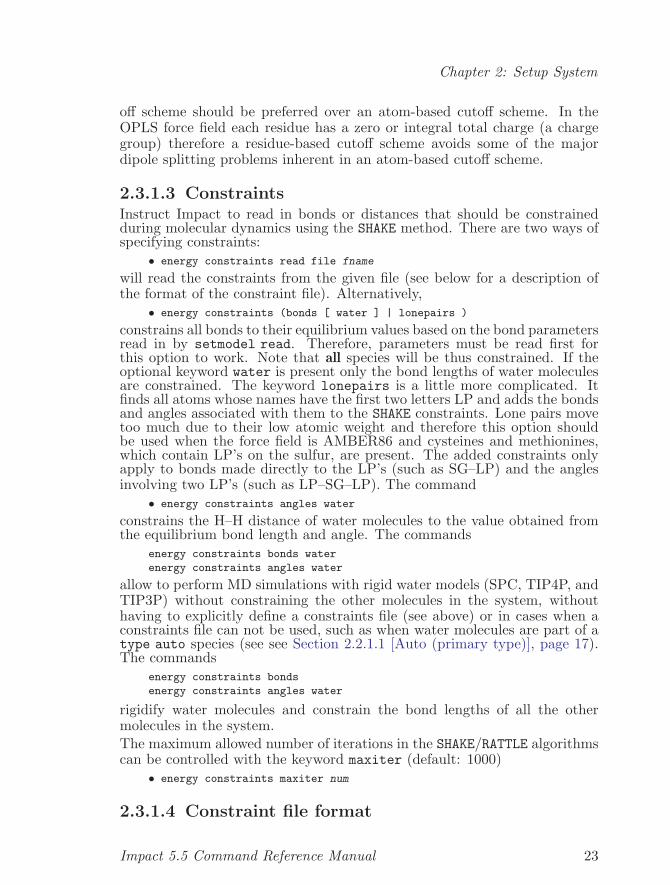
2.3.1.3 ConstraintsInstruct Impact to read in bonds or distances that should be constrainedduring molecular dynamics using the SHAKE method. There are two ways ofspecifying constraints:
• energy constraints read file fname
will read the constraints from the given file (see below for a description ofthe format of the constraint file). Alternatively,
• energy constraints (bonds [ water ] | lonepairs )
constrains all bonds to their equilibrium values based on the bond parametersread in by setmodel read. Therefore, parameters must be read first forthis option to work. Note that all species will be thus constrained. If theoptional keyword water is present only the bond lengths of water moleculesare constrained. The keyword lonepairs is a little more complicated. Itfinds all atoms whose names have the first two letters LP and adds the bondsand angles associated with them to the SHAKE constraints. Lone pairs movetoo much due to their low atomic weight and therefore this option shouldbe used when the force field is AMBER86 and cysteines and methionines,which contain LP’s on the sulfur, are present. The added constraints onlyapply to bonds made directly to the LP’s (such as SG–LP) and the anglesinvolving two LP’s (such as LP–SG–LP). The command
• energy constraints angles water
constrains the H–H distance of water molecules to the value obtained fromthe equilibrium bond length and angle. The commands
energy constraints bonds water
energy constraints angles water
allow to perform MD simulations with rigid water models (SPC, TIP4P, andTIP3P) without constraining the other molecules in the system, withouthaving to explicitly define a constraints file (see above) or in cases when aconstraints file can not be used, such as when water molecules are part of atype auto species (see see Section 2.2.1.1 [Auto (primary type)], page 17).The commands
energy constraints bonds
energy constraints angles water
rigidify water molecules and constrain the bond lengths of all the othermolecules in the system.The maximum allowed number of iterations in the SHAKE/RATTLE algorithmscan be controlled with the keyword maxiter (default: 1000)
• energy constraints maxiter num
2.3.1.4 Constraint file format
Impact 5.5 Command Reference Manual 23
Chapter 2: Setup System
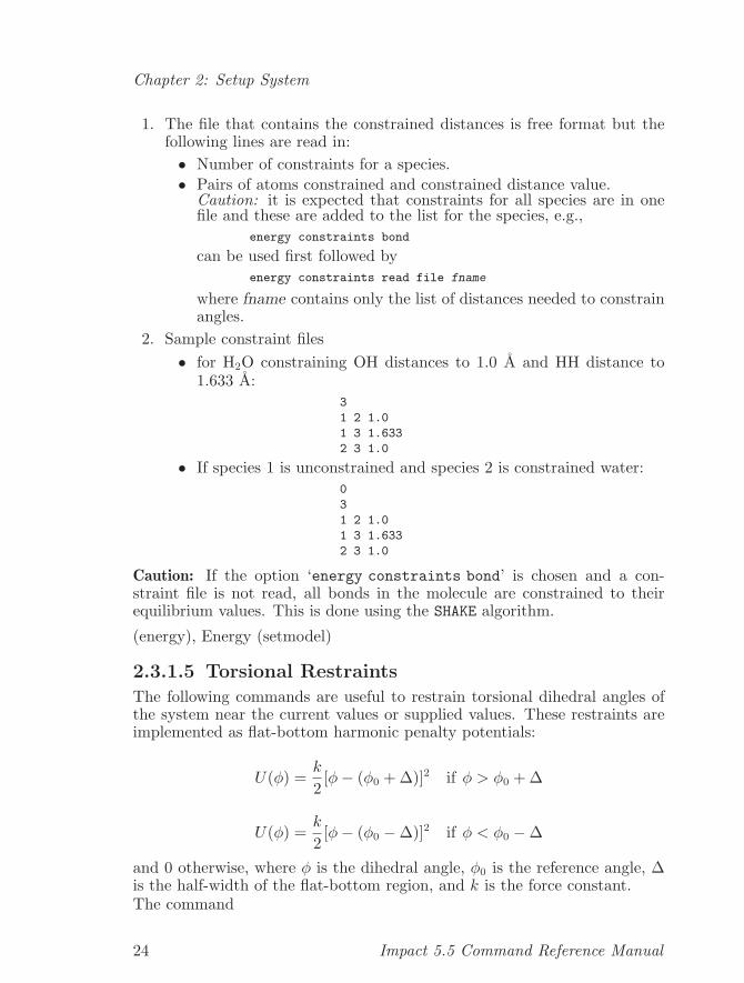
1. The file that contains the constrained distances is free format but thefollowing lines are read in:• Number of constraints for a species.• Pairs of atoms constrained and constrained distance value.
Caution: it is expected that constraints for all species are in onefile and these are added to the list for the species, e.g.,
energy constraints bond
can be used first followed byenergy constraints read file fname
where fname contains only the list of distances needed to constrainangles.
2. Sample constraint files• for H2O constraining OH distances to 1.0 A and HH distance to
1.633 A:3
1 2 1.0
1 3 1.633
2 3 1.0
• If species 1 is unconstrained and species 2 is constrained water:0
3
1 2 1.0
1 3 1.633
2 3 1.0
Caution: If the option ‘energy constraints bond’ is chosen and a con-straint file is not read, all bonds in the molecule are constrained to theirequilibrium values. This is done using the SHAKE algorithm.
(energy), Energy (setmodel)
2.3.1.5 Torsional Restraints
The following commands are useful to restrain torsional dihedral angles ofthe system near the current values or supplied values. These restraints areimplemented as flat-bottom harmonic penalty potentials:
U(φ) =k
2[φ− (φ0 + ∆)]2 if φ > φ0 + ∆
U(φ) =k
2[φ− (φ0 −∆)]2 if φ < φ0 −∆
and 0 otherwise, where φ is the dihedral angle, φ0 is the reference angle, ∆is the half-width of the flat-bottom region, and k is the force constant.The command
24 Impact 5.5 Command Reference Manual
Chapter 2: Setup System
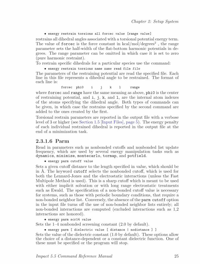
• energy restrain torsions all forcec value [range value]
restrains all dihedral angles associated with a torsional potential energy term.The value of forcec is the force constant in kcal/mol/degrees2 , the rangeparameter sets the half-width of the flat-bottom harmonic potentials in de-grees. The range parameter can be omitted in which case it is set to zero(pure harmonic restraint).To restrain specific dihedrals for a particular species use the command:
• energy restrain torsions name name read file file
The parameters of the restraining potential are read the specified file. Eachline in this file represents a dihedral angle to be restrained. The format ofeach line is:
forcec phi0 i j k l range
where forcec and range have the same meaning as above, phi0 is the centerof restraining potential, and i, j, k, and l, are the internal atom indexesof the atoms specifying the dihedral angle. Both types of commands canbe given, in which case the restrains specified by the second command areadded to the ones created by the first.Torsional restrain parameters are reported in the output file with a verboselevel of 3 or higher (see Section 1.5 [Input Files], page 5). The energy penaltyof each individual restrained dihedral is reported in the output file at theend of a minimization task.
2.3.1.6 ParmRead in parameters such as nonbonded cutoffs and nonbonded list updatefrequency, which are used by several energy manipulation tasks such asdynamics, minimize, montecarlo, tormap, and potfield.
• energy parm cutoff value
Sets a given cutoff distance to the length specified in value, which should bein A. The keyword cutoff selects the nonbonded cutoff, which is used forboth the Lennard-Jones and the electrostatic interactions (unless the FastMultipole Method is used). This is a sharp cutoff which is meant to be usedwith either implicit solvation or with long range electrostatic treatmentssuch as Ewald. The specification of a non-bonded cutoff value is necessaryfor systems, such as those with periodic boundary conditions, that require anon-bonded neighbor list. Conversely, the absence of the parm cutoff optionin the input file turns off the use of non-bonded neighbor lists entirely; allnon-bonded interactions are computed (excluded interactions such as 1,2interactions are honored).
• energy parm scr14 value
Sets the 1–4 nonbonded screening constant (2.0 by default).• energy parm [ dielectric value [ distance | nodistance ] ]
Sets the value of the dielectric constant (1.0 by default). These options allowthe choice of a distance-dependent or a constant dielectric function. One ofthese must be specified or the program will stop.
Impact 5.5 Command Reference Manual 25
Chapter 2: Setup System
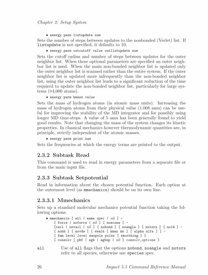
• energy parm listupdate num
Sets the number of steps between updates to the nonbonded (Verlet) list. Iflistupdate is not specified, it defaults to 10.
• energy parm outcutoff value outlistupdate num
Sets the cutoff radius and number of steps between updates for the outerneighbor list. When these optional parameters are specified an outer neigh-bor list is used. When the main non-bonded neighbor list is updated onlythe outer neighbor list is scanned rather than the entire system. If the outerneighbor list is updated more infrequently than the non-bonded neighborlist, using the outer neighbor list leads to a significant reduction of the timerequired to update the non-bonded neighbor list, particularly for large sys-tems (>4,000 atoms).
• energy parm hmass value
Sets the mass of hydrogen atoms (in atomic mass units). Increasing themass of hydrogen atoms from their physical value (1.008 amu) can be use-ful for improving the stability of the MD integrator and for possibly usinglonger MD time-steps. A value of 5 amu has been generally found to yieldgood results. Note that changing the mass of the system changes its kineticproperties. In classical mechanics however thermodynamic quantities are, inprinciple, strictly independent of the atomic masses.
• energy parm print num
Sets the frequencies at which the energy terms are printed to the output.
2.3.2 Subtask Read
This command is used to read in energy parameters from a separate file orfrom the main input file.
2.3.3 Subtask Setpotential
Read in information about the chosen potential function. Each option atthe outermost level (as mmechanics) should be on its own line.
2.3.3.1 Mmechanics
Sets up a standard molecular mechanics potential function taking the fol-lowing options.
• mmechanics [ all | name spec | nil ] -
[ force | noforce | nil ] [ noecons ] -
[tail | notail | nil ] [ nobond ] [ noangle ] [ notors ] [ no14 ] -
[ nohb ] [ novdw ] [ ewald [ kmax km ] [ alpha alfa ] ] -
[ fmm level level maxpole poles [ smoothing ] ]
[ consolv [ pbf | sgb | agbnp | nil ] consolv_options ]
all Use of all flags that the options nobond, noangle and notorsrefer to all species, otherwise use species spec.
26 Impact 5.5 Command Reference Manual
Chapter 2: Setup System
forcenoforce Force/noforce determine whether forces should be calculated.
Forces are required for minimization and dynamics. (This isthe default.) Currently this option is ignored if the Fast Multi-pole Method is used.
noecons Determines whether NOE (Nuclear Overhauser Effect) con-straints will be added to the potential (the default is no NOEconstraints).
tailnotail Determines whether long-range corrections to the van der Waals
energies due to cutoffs are made. Tail is needed for constantpressure simulations (the default is notail).
nobond Flag to turn off bond stretching term.
noangle Flag to turn off valence angle bending term.
notors Flag to turn off torsional twisting term.
no14 Flag to turn off both 1-4 interaction term (nonb14 and noel14).
noel Flag to turn off electrostatic term.
nohb Flag to turn off hydrogen bond term.
novdw Flag to turn off van der Waals (non-bonded) interaction term.
ewald Makes Impact use the Ewald summation method to handle thelong-range electrostatic interactions. It only works if all specieshave periodic boundary conditions. To describe the parametersfollowing the keywords kmax and alpha it is convenient to recallthe definition of the Ewald potential (with ‘conducting boundaryconditions’):
Φ(x) =∑n
erfc(α‖x + Ln‖)‖x + Ln‖
+∑k6=0
4πL3‖k‖2 exp
(−‖k‖
2
4α2 + ik · x)
− π
L3α2 .
This formula represents a solution to the Poisson equation fora unit charge under periodic boundary conditions (there is anegative background that renders the system neutral, as other-wise it can be shown that there is no solution) as a sum of twoinfinite series, both of which converge exponentially. The first,so-called ‘real-space sum’, converges faster the larger the valueof α is. Conversely, the second sum converges faster the smallerthis value. Impact restricts the first sum to the original copy,that is, it only considers the terms with n = 0. The second
Impact 5.5 Command Reference Manual 27
Chapter 2: Setup System
sum, the ‘reciprocal-space sum’, is restricted to those values ofk whose components are, in magnitude, less than or equal to theparameter specified by the keyword kmax (default: 5). The αparameter has by default the value 5.5/L, where L is the lin-ear dimension of the box (which must be cubic). The user canchange this value, however, with the alpha keyword. Note, how-ever, that changing this parameter might require changing themaximum number of reciprocal-space vectors also. A good refer-ence for the Ewald summation method is the book by Allen andTildesley, Computer Simulation of Liquids, Oxford UniversityPress, 1991. For the mathematically inclined we recommendalso the article: de Leeuw, Perram and Smith, Simulation ofelectrostatic systems in periodic boundary conditions. I. Latticesums and dielectric constants, Proc. R. Soc. London, A373,27–56 (1980).
fmm Selects the Fast Multipole Method (FMM) for the calculationof the electrostatic interactions. The number following levelshould be the desired number of levels in the hierarchical tree.Since the nodes of the tree correspond to subsequent subdivi-sions of the simulation box into halves along each direction, iflevel l is selected, the number of boxes at the lowest level willbe 8l and the linear dimension of each one box at that level willbe L/2l with L being the linear dimension of the simulation box(which must be cubic).The number following maxpole is the maximum number of mul-tipole moments that will be used to approximate the potentialand field produced by ‘far’ clusters. Currently a minimum of four(4) and a maximum of twenty (20) multipoles are allowed. Thekeyword smoothing determines whether a sharp or smooth cut-off are used to separate the direct forces into near and far com-ponents. It is only relevant when using the Reversible RESPAintegrators (see Section 3.2.2 [Dynamics Subtask Run], page 62)with more than two stages. If periodic boundary conditions arein effect, the potential that gets computed coincides with theEwald potential (see above), but the algorithm is completelydifferent. One important restriction when using the FMM withperiodic boundary conditions is that the system must be electri-cally neutral, i.e., the sum of all point charges must be zero. Themain reference for the FMM is Greengard’s thesis, The RapidEvaluation of Potential Fields in Particle Systems, The MITPress, Cambridge, 1988.Because FMM calculations scale linearly with the total num-ber of atoms, they can provide a significant speed advantage incalculating electrostatic interactions for large systems when it
28 Impact 5.5 Command Reference Manual
Chapter 2: Setup System
is not desirable to use cutoffs. Systems large enough for FMMto be advantageous may be large macromolecules or complexesof them, or smaller molecules with a large number of explicitsolvent molecules. If it is possible to impose periodic bound-ary conditions, then the Ewald method (which requires suchboundary conditions) tends to be faster than FMM for systemscontaining more than about 20000 atoms.PLEASE NOTE: The Fast Multipole Method cannot currentlybe used with the truncated Newton minimization algorithm(tnewton) (see Section 3.1.3 [Subtask Tnewton], page 56), orwith SGB continuum solvation (see below). It is available withPBF continuum solvation (see below), but the FMM is not ap-plied to the continuum solvent itself. Unless the solute is quitelarge, therefore, it may not be advantageous to use FMM withcontinuum solvent.
consolv [sgb]• mmechanics consolv sgb [ cutoff val ] -
[ npsolv ] [ debug val ]
SGB, the default option for consolv is a surface area based ver-sion of the Generalized Born model, which can be proved to bea well-defined approximation to the boundary element formula-tion of the Poisson-Boltzmann (PB) equation6. The relationshipof the surface area methodology to the volume-integration basedapproach of the original GB model7 can be found in Ghosh etal.’s paper. With empirical corrections, SGB produces signifi-cant improvements in accuracy, as compared to the uncorrectedGB model.PLEASE NOTE: This solvation method cannot currently beused with the Fast Multipole Method FMM (see above).
cutoff The cutoff parameter specifies how far any atommust move from the coordinates used in the previouscalculation before a new Reaction Field calculationis performed. The default value is 0.1 A. If all atomiccoordinates have moved less than this cutoff, thenthe previous calculated energy and forces are usedfor that step in the minimization. A relatively largevalue of cutoff can significantly reduce the requiredcomputational time at the expense of some loss inaccuracy.
npsolv The npsolv keyword will turn on the properlyparametrized dielectric radii and nonpolar param-
6 A. Ghosh, C. S. Rapp, and R. A. Friesner, J. Phys. Chem. B, 102, 10983, (1998)7 Still, et al. J. Am. Chem. Soc., 112, 6127, 1990
Impact 5.5 Command Reference Manual 29
Chapter 2: Setup System
eters for SGB continuum solvent simulations. Theparametrization was done by fitting the SGB cal-culated free energy coupled with a novel nonpolarfunction8 against small molecule experimental sol-vation free energies.
debug Setting debug to a nonzero value causes diagnosticmessages and files to be printed for each calculation.
The consolv sgb parameter files are in the directories$SCHRODINGER/impact-v5.5/data/opls
$SCHRODINGER/impact-v5.5/data/opls2000
and all start with sgb. The files should not need to be modifiedby the user on an ongoing basis; most useful parameters can bechanged via the sgbp input file keyword (see Section 2.3.4 [Sgbp(setmodel)], page 37).If the SGB model is activated, then the following line shouldappear in the output:
%IMPACT-I (mmstd): Using Surface Generalized Born Model
In the energy-decomposition printout provided by Impact dur-ing the course of a minimization, the continuum-solvent energyis provided under the heading ‘RxnFld(Sgb)’. These energiesinclude the interactions between the atomic-point charges andthe induced charges at the solute/solvent interface.Examples:
• mmechanics consolv sgb cutoff 0.1
• mmechanics consolv sgb nonpolar 1
consolv pbf• mmechanics consolv pbf [ pbfevery val ] [ cutoff val ] -
[ rxnf_cutoff val ] [ cavity_cutoff val ] -
[ low_res | med_res | high_res ] [ debug val ]
PBF is a Poisson-Boltzmann Solver. It takes as input a set ofatomic coordinates, their charges and radii, a solvent radius,and dielectric constants for the solute and solvent and computesthe electrostatic potential from the resulting Poisson-Boltzmannequation. The reaction-field energy (electrostatic interaction ofthe fixed atomic charges with the induced surface charges at thesolute/solvent interface) and gradient are then calculated. Thereaction-field terms effectively represent the average interactionbetween the solute molecule(s) and the solvent. The advantageof this approach is that the large number of solvent moleculestypically used in a solution-phase molecular simulation or min-imization are not required, thereby dramatically reducing the
8 E. Gallicchio, L. Y. Zhang, and R. M. Levy, J. Comput. Chem, 23, 517-529 (2002)
30 Impact 5.5 Command Reference Manual
Chapter 2: Setup System
computational expense. While treating the solvent as a contin-uum rather than a collection of discrete molecules is clearly anapproximation, it has been shown to be a fairly good one formany types of calculations.The novel feature of PBF over other algorithms used to solvethe Poisson-Boltzmann equation is the use of a finite-elementmesh with tetrahedron grids. This approach allows the densityof grid points used in solving the discretized equations to beoptimized such that accurate results may be achieved with aminimal number of grid points and hence with minimal compu-tational effort. For example, a high density of points is requiredat the solute/solvent interface to compute a accurate and numer-ically stable reaction-field gradient. Other approaches using, forinstance, a finite-difference method with cubic grids do not havethis flexibility and must use a large number of points to obtaincomparable accuracy. The use of a finite-element mesh also al-lows a high density of points to be used in a particular region ofinterest, e.g., a enzyme-binding site and a lower density of gridpoints elsewhere in the system, again minimizing the computa-tional effort.
pbfevery This parameter sets the frequency in timestepswhen a PBF calculation is performed. In betweentimesteps use the most recent PBF energies andforces.
cutoff The cutoff parameter specifies how far any atommust move from the coordinates used in the previ-ous calculation before a new Reaction Field calcula-tion is performed. The default value is 0.1 A. If allatomic coordinates have moved less than this cutoff,then the previous calculated energy and forces areused for that step in the minimization. Preliminaryresults suggest that the pbf energy and gradient areslowly varying functions of the atomic coordinates,relative to the other energies and forces involved ina typical molecular mechanics calculation. A rela-tively large value of cutoff can significantly reducethe required computational time at the expense ofsome loss in accuracy.
cavity_cutoffThe keyword cavity_cutoff is used for cavity termrecalculation. It is similar to the keyword cutoff.
low_res Use the low grid point resolution setting. This isthe default.
Impact 5.5 Command Reference Manual 31
Chapter 2: Setup System
med_res Use a medium grid point resolution setting.
high_res Use a high grid point resolution setting. This is themost expensive setting, but also the most accurate.
debug Setting debug to a nonzero value causes diagnosticmessages and files to be printed for each calculation.
The consolv pbf parameter files are in the directories$SCHRODINGER/impact-v5.5/data/opls
$SCHRODINGER/impact-v5.5/data/opls2000
and all start with pbf. The files should not need to be modifiedby the user on an ongoing basis. A few parameters, however,may need to be changed occasionally. For example, the dielectricconstants used for the solutes and solvent can be changed in the‘pbf.com’ file. Also the solvent radius can changed by editingthe same file.If the PBF model is activated, then the following line shouldappear in the output:
%IMPACT-I (mmstd): Using Poisson-Boltzmann Model
In the energy-decomposition printout provided by Impact dur-ing the course of a minimization, the continuum-solvent energyis provided under the heading ‘RxnFld(Pbf)’. These energiesinclude the interactions between the atomic-point charges andthe induced charges at the solute/solvent interface.Because of the large memory requirements for medium-sized andlarger proteins, PBF currently writes some arrays to disk andthen reads them back in as needed. Currently only one file isbeing written to disk, ‘zzZ_Ctbl_Pbf_Zzz’. Every effort is madeto remove this file after a calculation has completed. However,if a calculation is aborted or something goes amiss, this file maybe left on the disk.Examples:
• mmechanics consolv pbf cutoff 0.1
• mmechanics consolv pbf low_res cutoff 0.1 cavity_cutoff 0.9
consolv agbnp• mmechanics consolv agbnp
AGBNP is an analytical implicit solvent model based on thepairwise descreening (PD) Generalized Born (GB) model anda non-polar solvation free energy (NP) estimator which takesinto account independently the work of cavity formation and thesolute-solvent van der Waals interaction energy. The model andits derivation are described in detail in the following paper: E.Gallicchio, R. M. Levy, AGBNP: An Analytic Implicit SolventModel Suitable for Molecular Dynamics Simulations and High-Resolution Modeling, J. Comput. Chem., 25, 479-499 (2004).
32 Impact 5.5 Command Reference Manual
Chapter 2: Setup System
AGBNP is unique among pairwise descreening GB models inthat the overlap scaling coefficients depend on solute conforma-tion and are computed from purely geometric considerations,rather than being fit to experimental and Poisson Boltzmanndata. Hydrogen atoms do not contribute to descreening. Thenon-polar hydration free energy estimator is composed of twoterms. The first, related to the cavity hydration free energy,is proportional to the solute surface area of each atom throughsurface tension parameters that depend on atom type. The sur-face area is defined as the van der Waals surface area obtainedby increasing the van der Waals radius of each atom by 0.5 A.The surface area of each atom is calculated using an analyticalalgorithm based on the same method used to calculate overlapscaling factors. Hydrogen atoms do not contribute to the solutesurface area, that is they can be thought as of atoms of zeroradius in this respect. The second component of the non-polarhydration free energy model is a solute-solvent van der Waalsinteraction energy estimator that depends on the Born radiusand Lennard-Jones parameters of each atom. This estimatorincludes dimensionless scaling parameters for each atom typeadjusted to better reproduce solute-solvent van der Waals en-ergies obtained from explicit solvent simulations. In additionto the surface tension parameters and van der Waals scalingparameters, the other parameters of the model, atomic partialcharges and van der Waals radii, are derived from the under-lying force field without change (partial charges) or with smallmodifications (van der Waals radii).
The current AGBNP parameters are stored in a file calledagbnp.param in the directories
$SCHRODINGER/impact-v5.5/data/opls
$SCHRODINGER/impact-v5.5/data/opls2000
$SCHRODINGER/impact-v5.5/data/opls2001
$SCHRODINGER/impact-v5.5/data/opls2005
depending on the active force field version. The format of theagbnp.param file is as follows:
Impact 5.5 Command Reference Manual 33
Chapter 2: Setup System
Column Content1 Type index2 OPLS symbolic type3 van der Waals radius [A]4 non-polar gamma parameter [(kcal/mol)/A2]5 non-polar alpha parameter [dimensionless]6 non-polar delta parameter [kcal/mol]7 correction gamma parameter [(kcal/mol)/A2]8 correction alpha parameter [dimensionless]9 correction delta parameter [kcal/mol]10 screening parameter [dimensionless]
Lines that begin with ’#’ are comments. Lines beginning withdielectric_in and dielectric_out set the dielectric solventof the solute and the solvent, respectively, and should precedeany other non-comment line. gamma above refers to the surfacetension parameters, alpha to the solute-solvent van der Waalsscaling parameters, the values of the delta parameters shouldbe left to their default values (zero). The values of the non-polar parameters used internally are the sum of the pure andcorrection values. However the non-polar energy derived fromeach is reported separately as a pure non-polar energy and a cor-rection energy term. The correction energy term has the sameexpression as the non-polar estimator (this could change in thefuture) but it is calculated using the set of correction parame-ters rather than the pure non-polar parameters. The screeningparameter in column 10, normally set to 1 for all atom types, isdescribed in the following paper: A. K. Felts, Y. Harano, E. Gal-licchio, and R. M. Levy. Free energy surfaces of beta-hairpin andalpha-helical peptides generated by replica exchange moleculardynamics with the AGBNP implicit solvent model. PROTEINS:Structure, Function, and Bioinformatics, 56, 310-321 (2004). Tomodify the AGBNP parameters edit a copy of the agbnp.paramfile in the working directory. The agbnp.param file in the work-ing directory takes precedence over the agbnp.param file in thedata directory.If the AGBNP model is activated the following line should ap-pear in the output:
%IMPACT-I: Using AGBNP: Analytical Generalized Born Model + Analytic
Non-Polar Hydration Model
The running AGBNP energy components are reported under thelabels RxnFld(AGBNP) and NPolar(AGBNP) in the output file, forthe electrostatic and non-polar components (pure plus correc-tion) respectively. The energy summary at the end of the out-put file lists the total AGBNP solvation free energy under AGBNPSolvation Energy, the electrostatic component of the solva-tion free energy under AGBNP Solvation Energy (polar), the
34 Impact 5.5 Command Reference Manual
Chapter 2: Setup System
pure non-polar component under AGBNP Solv. Energy (non-polar), and the correction term under AGBNP Solv. Energy(correction).There are no options associated with the consolv agbnp set-ting. AGBNP applies the same distance cutoff as specified bythe energy parm cutoff command (see Section 2.3.1.6 [Parm(energy)], page 25) for the GB pair energies and for the pairwisedescreening calculation of Born radii.
2.3.3.2 Mmechanics Pff
Set up a polarizable force field potential function. Only a few of the optionsdescribed in Section 2.3.3.1 [Mmechanics (setpotential)], page 26 are appro-priate for use with PFF. For more information on the theory, see Section 1.7.2[PFF (ffield)], page 12. In order to use the PFF, you must also specify SETFFIELD OPLS_PFF_2000 or OPLS_PFF_2005 (see Section 2.1.2 [Ffield (set)],page 15).The PFF module is only available under special license from Schrodinger.
• mmechanics pff [ consolv pbf npsolv ]
PFF calculations should always use a large enough cutoff to encompass theentire system.
consolv pbf npsolvUse the parameterized PBF continuum solvent model with thepolarizable force field potential function. The PBF and non-polar models are in Section 2.3.3.1 [Mmechanics (setpotential)],page 26, but the nonpolar parameterization used here is opti-mized for PFF.Caution: The keywords pbf and npsolv should always be usedwith pff consolv as their parameterizations are coupled.
The corresponding parameter file to be read in must be ‘parampff.dat’ inthe read parm subtask, such as in the following example:
SETMODEL
setpotential
mmechanics pff consolv pbf npsolv
quit
read parm file parampff.dat noprint
energy parm cutoff 100.0 listupdate 10 diel 1.0 nodist
QUIT
2.3.3.3 Weight
Change the weights of terms in the potential function. Unless otherwiseindicated below, the weights are all initialized to 1.0 when mmechanics isused.
Impact 5.5 Command Reference Manual 35
Chapter 2: Setup System
Caution: Despite the terminology below, intramolecular nonbond terms areaffected both by intramolecular and intermolecular electrostatic and LJweights. The total nonbond weight is the product of the intramolecular(within one species) and intermolecular (between species) weights.
• weight intramolecular name spec -
[ bond | angle | torsion | el14 | lj14 | elin | ljin | hbin ] weight
The intramolecular keyword is used to change the weights of intramolecu-lar terms (those within a single species). The elin, ljin, and hbin keywordschange the weights for all included nonbond pairs within the molecule; el14and lj14 change them only for “1-4” pairs, i.e., atoms at the outer ends of aquartet that defines a torsion angle. hbin is only used with the AMBER86force field.
• weight intermolecular -
[ vdw | eel | hbond | hbelectrostatics ] weight
The intermolecular keyword is used to change the weights of intermolecu-lar terms within or between species, thus there is no name spec designation.hbond and hbelectrostatics are only used with the AMBER86 force field.
• weight constraints name spec -
[ noe | torsion | hbond ] weight
• weight constraints name spec buffer weight -
[ halfwidth sigma ]
The constraints keyword defines the weights of various restraint force con-stants terms. The noe, torsion, and hbond terms are zero by default anddefine NOE distance and torsion restraint weights.The buffer constraint energy is a harmonic term is applied to all “buffered”atoms specified via zonecons commands. See Section 2.3.7 [Zonecons (set-model)], page 40. The default buffer is 25 kcal/(A2 mol). You can controlthe sigma halfwidth value via the halfwidth keyword, whose default is 0.0,equivalent to a harmonic constraint.Caution: buffer is not a per-species parameter, but is applied to all bufferedatoms in the system.
2.3.3.4 ConstraintsRead in distance and torsional constraint lists from a file or the main inputfile.
• constraints name spec noec distance -
con1 num con2 num -
[ file fname ]
• constraints name spec noec torsion -
nsec num_sections -
( fres num lres num tpsi value -
tphi value range value ) repeated num sections times
distance signals that distance constraints will be read in.
torsion signals that torsion constraints will be read in.
36 Impact 5.5 Command Reference Manual
Chapter 2: Setup System
file name of constraint file (if different from main input file). Thisfile has the following 6 or 7 fields—in order but free format: (theindividual NOE weight is optional see Notes below)resn atna resn atna lower bound upper bound noe weight
con1 number of H-H distance constraints, type 1, to read in.
con2 number of distance constraints between heavy atoms, type 2, toread in.
If prochiral assignments can be made and you know theconstraint is between HB1-HG2 then the atoms namesshould be specified as such and no averaging over equiv-alent hydrogens will be implemented.If prochiral assignments can not be made (or in the caseof equivalent H atoms on methyl groups) you need to spec-ify only the character part of the atom name. In this caseaveraging over equivalent hydrogens is automatically imple-mented, ie., for a methylene proton-methyl group interac-tion.1. HB1-HG will result in no averaging on the methylene
but the methyl group will be averaged2. HB-HG will result in averaging over the protons in the
methylene group and the protons in the methyl group.
Number of sections of torsions to be constrained.
tphi Target value for φ angles (for constraining proteinsecondary structure).
tpsi Target value for ψ values (for constraining proteinsecondary structure).
range Allowed range (i.e., constraint will be tphi ± rang).
ncon Number of constraints to be read explicitly.These keywords are read in free format nsec times 4(res. no., atom name)target value, range. Caution: The weight for the individual NOE constraintis multiplied by the weight for the entire NOE term. It is one by default andcan be set to any arbitrary value except zero.
2.3.4 Subtask Sgbp
This keyword sets various SGB continuum solvent simulation parameters.It has no effect unless mmechanics consolv sgb is used in a precedingsetpotential subtask to activate the SGB method.
• sgbp grid_size max dock_grid_size glide_max -
min_grid_size min printe [0|1] printf [0|1] -
active_reg_incr val buffer_reg_size val accuracy val -
epsout val hydrogen_radius val
Impact 5.5 Command Reference Manual 37
Chapter 2: Setup System
grid_sizeThe maximum number of grid points each atom can have. Thedefault value is 70.
dock_grid_sizeIn a Glide calculation, the maximum number of grid points eachatom can have, the default is 30.
min_grid_sizeThe minimum number of grid points each atom can have. Thedefault value is 20.
printe If set to 1, print the SGB energy. The default is 0.
printf If set to 1, print the SGB forces. The default is 0.
active_reg_incrWhen setting up the active region region, this amount is addedto it. The default is 0.
buffer_reg_sizeThis defines the buffer region size; the buffer region is locatedbetween the active region and the frozen region.
accuracy The threshhold value used with the singlelong multiple timescale scheme, and is related to the number of surface grid pointsused. The default value is 0.00001. Smaller values result indenser grids.
epsout The exterior (solvent) dielectric constant. The default is 80.0,a value typical of water simulations. (The interior dielectricconstant is set by enrg parm diel, see Section 2.3.1.6 [Parm(energy)], page 25.)
hydrogen_radiusThe atomic radius of hydrogen, used in generating the surface.The default value is 1.0.
2.3.5 Subtask Mixture• mixture [ density val | keep num ] [ overlap val]
This command sets optional parameters for the removal of excess solventmolecules when solvent and solute are mixed. If mixture is not present thenthe default is to remove all solvent molecules that overlap (as defined below)with any solute atom. When the mixture command is issued only up to amaximum of N solvent molecules are removed. N is calculated in one oftwo ways. Either from the effective solute volume (which can be controlledusing the density parameter) or from the number of solvent molecules notto be removed (the keep parameter). A molecule is considered for removalif the ratio of the distance d and the sum R1+R2 of the van der Waals radii
38 Impact 5.5 Command Reference Manual
Chapter 2: Setup System
of any atom of the solvent molecule and any atom of the solute is smallerthan a overlap threshold value (the overlap parameter). If the minimumdistance d is larger than 10 A a solvent molecule is not considered for removalregardless of the value of the overlap threshold value. If more than N solventmolecules are flagged for removal only the N solvent molecules with thesmallest minimum distance d are removed. If instead the number of solventmolecules flagged for removal is less than N all flagged solvent molecules areremoved.
density Keyword density is used to set the solute density. The default is1 g/cm3. The volume of solvent removed is equal to the effectivevolume of the solute. The effective solute volume is calculatedfrom the solute mass and the solute density. The larger thesolute density the smaller the effective solute volume and thusthe smaller the maximum number N of solvent molecules to beremoved.
keep Keyword keep is used to set explicitly the minimum number ofsolvent molecules remaining after removal. The default is 0. Themaximum number N of solvent molecules to be removed is setas the current number of solvent molecules minus the numberof solvent molecules to keep. The keep option preempts thedensity option if both are given.
overlap The overlap option is used to set the overlap threshold valuebelow which a solvent atom is considered to overlap with a soluteatom. The default is 1. Decreasing the overlap parameter makesit less likely for two atoms to overlap.
2.3.6 Subtask Solute
This subtask is used to place solute molecules at certain positions in thecontainer “box” of solvent used for the simulations.
2.3.6.1 TranslateThe keyword translate brings the center of mass (COM) of the system ofsolute molecules to the origin (center of the box), and also finds the longestdistance between atoms along the principal axis, which determines the boxedge lengths. The option skip says to ignore the last num residues of thesolute when performing the operation. With rotate, the solute is rotatedso that the principal moments of inertia coincide with the x, y, z axis. Thelongest axis of the molecule is oriented along the z axis. Skip has the abovemeaning. If rotate diagonal is given on the command line the rotationis such that the principal moment of inertia lies along the diagonal of thesimulation box (which must be cubic for this option to work).
• solute translate [ rotate [ diagonal ] ] name spec [ skip num ]
Caution: skip num excludes residues that may not have meaningful coor-dinates yet (such as counterions) from the translation/rotation operation.
Impact 5.5 Command Reference Manual 39
Chapter 2: Setup System
This parameter may be read in for as many different species as necessary.The value given for skip means that the last num residues of the species areignored in the translation/rotation of the solute.
2.3.7 Subtask ZoneconsThis subtask is used to constrain (freeze) or restrain (buffer) various regionsof a molecule based on options specified by the user.
• zonecons [ auto | [ [freeze|genbuffer] | chain | resseq | -
residue | atom | sphere ] name spec sub-options ]
There are seven types of zonecons subtasks described below. All butzonecons auto are additive, so you can use combinations of them. By de-fault, all atoms are free to move, as if there are no zonecons subtasks atall.Any buffered atoms are restrained using an harmonic potential centered onthe original atom position. Any atom position can be restrained this way.A buffer zone is often used to to define an intermediate zone between a fixedregion where the atom positions are frozen and the free region where theatom positions are not restrained. The buffer option is also often used toperform constrained minimizations. The force constant of the restrainingharmonic potential is user selectable, see Section 2.3.3.3 [Weight (setpoten-tial)], page 35.
2.3.7.1 AutoUse the frozen/buffered settings from an input Maestro file.
• zonecons auto
Maestro files written by Maestro specifically for Glide, Liaison, or QSite jobs,or written as output from a Glide, Liaison, or QSite job, will contain an extraparameter (internally named i_i_constraint) for each atom. Zoneconsauto uses this parameter in lieu of any other zonecons option, where thevalues 0, 1, and 2 correspond to free, frozen, and buffered, respectively.
2.3.7.2 Freeze/Genbuffer
Freeze or restrain (buffer) a specified group of atoms, e.g., all heavy atoms,all C atoms, all N atoms, all O atoms, or all atoms.
• zonecons [freeze|genbuffer] name spec [all | allC | allN | allO | allheavy]
This is the general freezing or restraining option, it can be used tofreeze/restrain all atoms, all carbon atoms, all nitrogen atoms, all oxy-gen atoms, or all heavy atoms. The general restraining option is calledgenbuffer to differentiate it from the buffer designation available in someof the other zonecons options.
2.3.7.3 ChainChain-based scheme, select any chain in a protein to be in fixed, free, orbuffer region
40 Impact 5.5 Command Reference Manual
Chapter 2: Setup System
• zonecons chain name spec [chainname name [fixed|free|buffer] ]+
This is the chain option, which is used to classify the whole chain with nameto be in fixed, free, or buffer regions.
2.3.7.4 ResseqResidue sequence-based scheme, such as from residue number 20 to 50, tobe in fixed, free, or buffer region
• zonecons resseq name spec [resn fres to lres -
[all | allC | allN | allO | allheavy] [fixed|free|buffer] ]+
This is the residue sequence option, which states that in the specified residuesequence, starting from first residue fres to last residue lres, the specifiedatom types (all atoms, all carbons, etc.) are to be in fixed or free or bufferregions.
2.3.7.5 ResidueResidue-based scheme, such as backbone, sidechain, or amide of a residue tobe in fixed, free, or buffer region
• zonecons residue name spec [resn num -
[all|backbone|sidechain|amide|Calpha|Ncap|Ccap] [fixed|free|buffer] ]+
This is the residue option, which states that in the specified individualresidue(s), with residue number(s) num, the specified atoms (all, backbone,sidechain, amide, α carbon, etc.) are to be in fixed or free or buffer regions.
2.3.7.6 AtomAtom-based scheme, for any particular atom
• zonecons atom name spec [atmn num [fixed|free|buffer] resadj [0|1] ]+
The atom option, the lowest level option, which classifies each atom to bein the fixed or free or buffer regions.The option resadj is used for residue-based adjustment; if it equals 1, thenthe whole residue associated with that particular atom will be classified inthe the same region (in this case the residue becomes the basic operationalunit). The default value for resadj is 0, which means no residue-basedadjustment is performed.
2.3.7.7 SphereSphere-based scheme, freeze/relax any atoms inside a sphere with a centerand radius
• zonecons sphere [center x val y val z val | name spec resn num atom-
name name] -
[freeze | relax ] rad rad buffrad buffrad resadj [1|0]
This is the sphere option, which is used to relax or freeze a sphere with thecenter located at residue number num and atom name name, and a radiusof rad. The buffrad is the radius for buffer, the shell between radius rad and
Impact 5.5 Command Reference Manual 41
Chapter 2: Setup System
buffrad becomes the buffer region. It should be noted that buffrad shouldbe bigger or equal than rad.The option resadj has the same meaning as in the atom option, except thedefault value here is 1, which means the residue-based adjustment is turnedon in sphere option by default.
2.3.7.8 Example Zonecons Input
Here is an example for how to use the various options for zone constraints.setmodel
setpotential
mmechanics
quit
read parm file paramstd.dat noprint
enrg parm cutoff 20.0 -
listupdate 100 diel 1.0 nodist print 1
zonecons freeze name hiv allheavy
zonecons chain name hiv chainname A free chainname B fixed
zonecons sphere name hiv resn 20 atomname CA relax rad 10.0 buffrad 12.0
zonecons residue name hiv resn 10 backbone fixed resn 11 sidechain free
zonecons resseq name hiv resn 20 to 40 all buffer resn 41 to 100 all fixed
zonecons atom name hiv atmn 45 free atmn 50 fixed atmn 52 buffer
quit
2.3.7.9 Zonecons Keywords
Some of the keywords used above for various zonecons subtasks have thefollowing meanings. Not all keywords are appropriate for every zoneconsoption, see the above syntax diagrams for a list of those allowed.
freeze General freeze option, to freeze all atoms, all carbons or all heavyatoms.
chain Chain option, to freeze/relax/buffer proteins by chain name.
resseq Residue sequence option, to freeze/relax/buffer proteins byresidue sequence.
residue Residue option, to freeze/relax/buffer a residue’s backbone,sidechain, etc.
atom Atom option, to freeze/relax/buffer any particular atom.
sphere Sphere option, to freeze/relax a sphere with a center and a ra-dius.
free Free to move.
buffer In the buffer region.
fixed In the frozen region.
42 Impact 5.5 Command Reference Manual
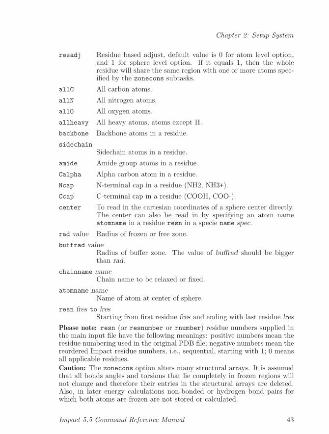
Chapter 2: Setup System
resadj Residue based adjust, default value is 0 for atom level option,and 1 for sphere level option. If it equals 1, then the wholeresidue will share the same region with one or more atoms spec-ified by the zonecons subtasks.
allC All carbon atoms.
allN All nitrogen atoms.
allO All oxygen atoms.
allheavy All heavy atoms, atoms except H.
backbone Backbone atoms in a residue.
sidechainSidechain atoms in a residue.
amide Amide group atoms in a residue.
Calpha Alpha carbon atom in a residue.
Ncap N-terminal cap in a residue (NH2, NH3+).
Ccap C-terminal cap in a residue (COOH, COO-).
center To read in the cartesian coordinates of a sphere center directly.The center can also be read in by specifying an atom nameatomname in a residue resn in a specie name spec.
rad value Radius of frozen or free zone.
buffrad valueRadius of buffer zone. The value of buffrad should be biggerthan rad.
chainname nameChain name to be relaxed or fixed.
atomname nameName of atom at center of sphere.
resn fres to lresStarting from first residue fres and ending with last residue lres
Please note: resn (or resnumber or rnumber) residue numbers supplied inthe main input file have the following meanings: positive numbers mean theresidue numbering used in the original PDB file; negative numbers mean thereordered Impact residue numbers, i.e., sequential, starting with 1; 0 meansall applicable residues.Caution: The zonecons option alters many structural arrays. It is assumedthat all bonds angles and torsions that lie completely in frozen regions willnot change and therefore their entries in the structural arrays are deleted.Also, in later energy calculations non-bonded or hydrogen bond pairs forwhich both atoms are frozen are not stored or calculated.
Impact 5.5 Command Reference Manual 43
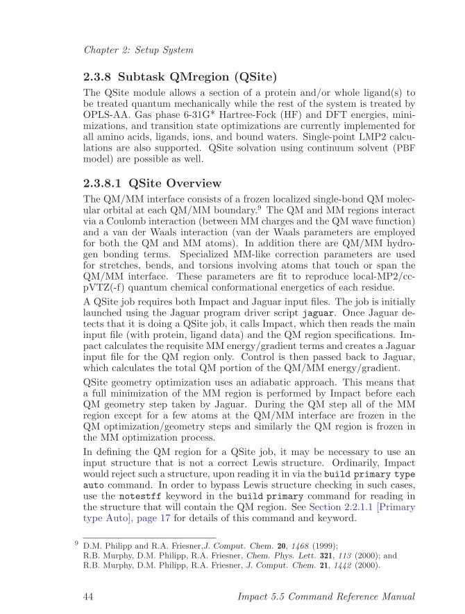
Chapter 2: Setup System
2.3.8 Subtask QMregion (QSite)
The QSite module allows a section of a protein and/or whole ligand(s) tobe treated quantum mechanically while the rest of the system is treated byOPLS-AA. Gas phase 6-31G* Hartree-Fock (HF) and DFT energies, mini-mizations, and transition state optimizations are currently implemented forall amino acids, ligands, ions, and bound waters. Single-point LMP2 calcu-lations are also supported. QSite solvation using continuum solvent (PBFmodel) are possible as well.
2.3.8.1 QSite Overview
The QM/MM interface consists of a frozen localized single-bond QM molec-ular orbital at each QM/MM boundary.9 The QM and MM regions interactvia a Coulomb interaction (between MM charges and the QM wave function)and a van der Waals interaction (van der Waals parameters are employedfor both the QM and MM atoms). In addition there are QM/MM hydro-gen bonding terms. Specialized MM-like correction parameters are usedfor stretches, bends, and torsions involving atoms that touch or span theQM/MM interface. These parameters are fit to reproduce local-MP2/cc-pVTZ(-f) quantum chemical conformational energetics of each residue.A QSite job requires both Impact and Jaguar input files. The job is initiallylaunched using the Jaguar program driver script jaguar. Once Jaguar de-tects that it is doing a QSite job, it calls Impact, which then reads the maininput file (with protein, ligand data) and the QM region specifications. Im-pact calculates the requisite MM energy/gradient terms and creates a Jaguarinput file for the QM region only. Control is then passed back to Jaguar,which calculates the total QM portion of the QM/MM energy/gradient.QSite geometry optimization uses an adiabatic approach. This means thata full minimization of the MM region is performed by Impact before eachQM geometry step taken by Jaguar. During the QM step all of the MMregion except for a few atoms at the QM/MM interface are frozen in theQM optimization/geometry steps and similarly the QM region is frozen inthe MM optimization process.In defining the QM region for a QSite job, it may be necessary to use aninput structure that is not a correct Lewis structure. Ordinarily, Impactwould reject such a structure, upon reading it in via the build primary typeauto command. In order to bypass Lewis structure checking in such cases,use the notestff keyword in the build primary command for reading inthe structure that will contain the QM region. See Section 2.2.1.1 [Primarytype Auto], page 17 for details of this command and keyword.
9 D.M. Philipp and R.A. Friesner,J. Comput. Chem. 20, 1468 (1999);R.B. Murphy, D.M. Philipp, R.A. Friesner, Chem. Phys. Lett. 321, 113 (2000); andR.B. Murphy, D.M. Philipp, R.A. Friesner, J. Comput. Chem. 21, 1442 (2000).
44 Impact 5.5 Command Reference Manual
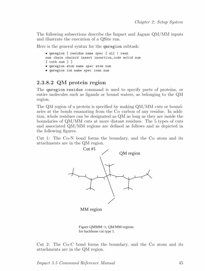
Chapter 2: Setup System
The following subsections describe the Impact and Jaguar QM/MM inputsand illustrate the execution of a QSite run.
Here is the general syntax for the qmregion subtask:• qmregion [ residue name spec [ all | resn
num chain chainid insert insertion_code molid num
[ cutb num ] ]
• qmregion atom name spec atom num
• qmregion ion name spec ionn num
2.3.8.2 QM protein region
The qmregion residue command is used to specify parts of proteins, orentire molecules such as ligands or bound waters, as belonging to the QMregion.
The QM region of a protein is specified by making QM/MM cuts or bound-aries at the bonds emanating from the Cα carbon of any residue. In addi-tion, whole residues can be designated as QM as long as they are inside theboundaries of QM/MM cuts at more distant residues. The 5 types of cutsand associated QM/MM regions are defined as follows and as depicted inthe following figures.
Cut 1: The Cα-N bond forms the boundary, and the Cα atom and itsattachments are in the QM region.
QM region
MM region
Cut #1
Figure QMMM−1; QM/MM regionsfor backbone cut type 1.
Cut 2: The Cα-C bond forms the boundary, and the Cα atom and itsattachments are in the QM region.
Impact 5.5 Command Reference Manual 45
Chapter 2: Setup System
QM region
MM regionCut #2
Figure QMMM−2; QM/MM regionsfor backbone cut type 2.
Cut 3: The Cβ-Cα bond forms the boundary, and the side chain is the QMregion.
QM region
MM region
Cut #3
Figure QMMM−3; QM/MM regions for side chain cut type 3.
Cut 4: The N-Cα bond forms the boundary, and the amide nitrogen (N)and its attachments are in the QM region.
46 Impact 5.5 Command Reference Manual
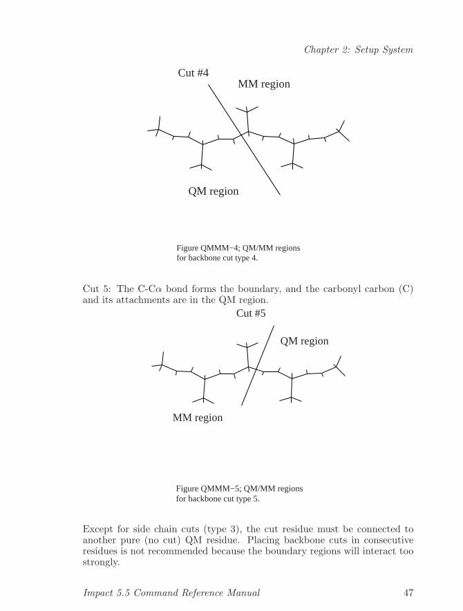
Chapter 2: Setup System
QM region
MM regionCut #4
Figure QMMM−4; QM/MM regionsfor backbone cut type 4.
Cut 5: The C-Cα bond forms the boundary, and the carbonyl carbon (C)and its attachments are in the QM region.
QM region
MM region
Cut #5
Figure QMMM−5; QM/MM regionsfor backbone cut type 5.
Except for side chain cuts (type 3), the cut residue must be connected toanother pure (no cut) QM residue. Placing backbone cuts in consecutiveresidues is not recommended because the boundary regions will interact toostrongly.
Impact 5.5 Command Reference Manual 47
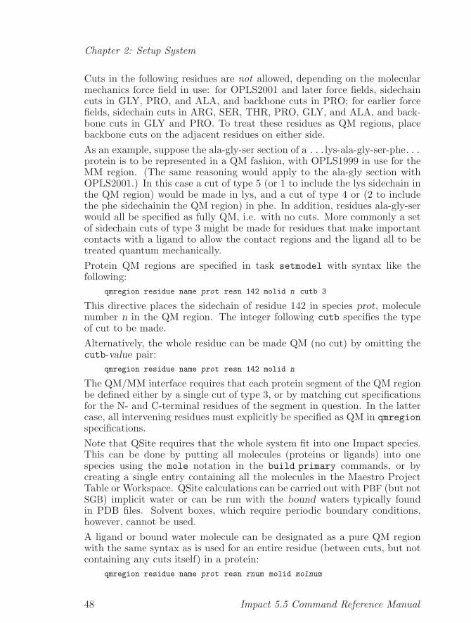
Chapter 2: Setup System
Cuts in the following residues are not allowed, depending on the molecularmechanics force field in use: for OPLS2001 and later force fields, sidechaincuts in GLY, PRO, and ALA, and backbone cuts in PRO; for earlier forcefields, sidechain cuts in ARG, SER, THR, PRO, GLY, and ALA, and back-bone cuts in GLY and PRO. To treat these residues as QM regions, placebackbone cuts on the adjacent residues on either side.As an example, suppose the ala-gly-ser section of a . . . lys-ala-gly-ser-phe. . .protein is to be represented in a QM fashion, with OPLS1999 in use for theMM region. (The same reasoning would apply to the ala-gly section withOPLS2001.) In this case a cut of type 5 (or 1 to include the lys sidechain inthe QM region) would be made in lys, and a cut of type 4 or (2 to includethe phe sidechainin the QM region) in phe. In addition, residues ala-gly-serwould all be specified as fully QM, i.e. with no cuts. More commonly a setof sidechain cuts of type 3 might be made for residues that make importantcontacts with a ligand to allow the contact regions and the ligand all to betreated quantum mechanically.Protein QM regions are specified in task setmodel with syntax like thefollowing:
qmregion residue name prot resn 142 molid n cutb 3
This directive places the sidechain of residue 142 in species prot, moleculenumber n in the QM region. The integer following cutb specifies the typeof cut to be made.Alternatively, the whole residue can be made QM (no cut) by omitting thecutb-value pair:
qmregion residue name prot resn 142 molid n
The QM/MM interface requires that each protein segment of the QM regionbe defined either by a single cut of type 3, or by matching cut specificationsfor the N- and C-terminal residues of the segment in question. In the lattercase, all intervening residues must explicitly be specified as QM in qmregionspecifications.Note that QSite requires that the whole system fit into one Impact species.This can be done by putting all molecules (proteins or ligands) into onespecies using the mole notation in the build primary commands, or bycreating a single entry containing all the molecules in the Maestro ProjectTable or Workspace. QSite calculations can be carried out with PBF (but notSGB) implicit water or can be run with the bound waters typically foundin PDB files. Solvent boxes, which require periodic boundary conditions,however, cannot be used.A ligand or bound water molecule can be designated as a pure QM regionwith the same syntax as is used for an entire residue (between cuts, but notcontaining any cuts itself) in a protein:
qmregion residue name prot resn rnum molid molnum
48 Impact 5.5 Command Reference Manual
Chapter 2: Setup System
where residue number rnum, in molecule number molnum, denotes the de-sired molecule in species prot. This syntax (with no cutb specification) des-ignates the whole molecule as a QM region. Note that QM/MM boundariescannot currently be made between ligand atoms.
2.3.8.3 Individual QM Atoms
The syntaxqmregion atom name spec atom num
indicates that the individual atom number num in species spec is to beincluded in the QM region.
2.3.8.4 QM Ions
Ions can be included in the QM region first by building the ion or ions. Thefollowing illustrates the placement of a Zn2+ ion:
CREATE
...
build newres zn2+ file zn
build primary ions name prot zn 1 xyz x 36.921 y 44.908 z -7.111 end
...
where build newres creates a Zn2+ residue with the name zn (the 1 followingzn is a specification for one ion), and build primary ions adds the ion intothe previously defined molecule of the species prot at coordinates (x,y,z).The specification of the ion as a QM region is done as follows:
qmregion ion name prot ionn 1
specifies that ion number (ionn) “1” of species prot should be treated asa QM ion. When multiple ions are present, one such qmregion directiveshould be given for each ion that is to be QM.
2.3.8.5 Basis set specifications.
All of the standard basis sets used in Jaguar are available for the QM regionof a QSite setup. Then basis sets can be specified within the Impact inputas follows.
• basis name spec [ atom num | resnumber num | nil ] [ radius rad ] basis bset
The default basis used is 6-31G* (LACVP* for metals), which must be en-tered into the Jaguar input file (see below) regardless of other basis setspecifications. To specify the basis on a particular residue the followingsyntax applies:
SETMODEL
..
qmregion residue name dipep resn 2 cutb 3
..
basis name dipep resnumber 2 basis cc-pvtz(-f)
..
QUIT
Impact 5.5 Command Reference Manual 49
Chapter 2: Setup System
This will setup a cc-pvtz(-f) basis on the QM atoms of previously speci-fied QM residue 2. Note that atoms comprising the QM/MM cut and theirbonded neighbors will automatically stay at 6-31G*. This restriction is nec-essary since the QM/MM boundary region is parametrized with 6-31G*.The code will automatically keep the necessary 6-31G* basis sets regardlessof basis set specifications made by the user.
The syntax for changing the basis set within a specified radius of a chosenatom is:10
SETMODEL
..
qmregion residue name dipep resn 2 cutb 3
..
basis name dipep atom 34 radius 5.0 basis cc-pvtz(-f)
..
QUIT
will change the basis set to cc-pvtz(-f) on atoms within 5 A of atom number34. This atom must be in a residue or a ligand in the QM region as specifiedby the qmregion commands.
2.3.8.6 QSite energy/minimization:
Single point QSite energies can be obtained using task analysis with thesubtask qmme, e.g.,
ANALYSIS
qmme
QUIT
will tell Impact to generate a QM/MM energy.
QSite geometry optimizations require the usual Impact MM minimizationsection, e.g.:
MINM
conjugate dx0 0.05 dxm 3.0 rest 50
input cntl mxcyc 10000 rmscut 1.9e-1 deltae 0.5
run
QUIT
with no special QSite flags.
The following Impact example, and the Jaguar input example below, are fora small polypeptide with a water molecule. A threonine residue and watermolecule constitute the QM region and are treated at the B3LYP level. Therest of the structure is treated with molecular mechanics.
10 N.B.: The radius option is not available via Maestro, but you can add it by hand into theinput file
50 Impact 5.5 Command Reference Manual
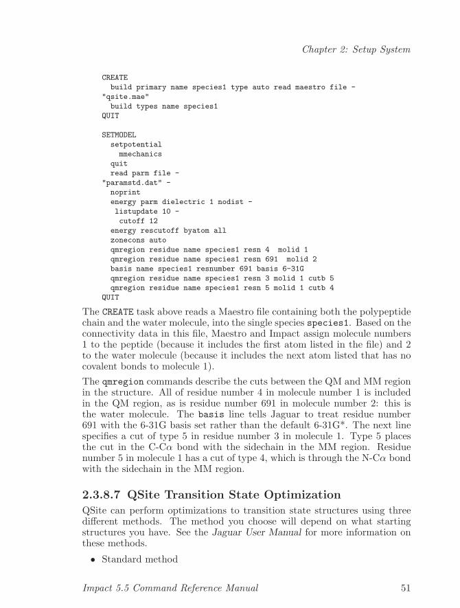
Chapter 2: Setup System
CREATE
build primary name species1 type auto read maestro file -
"qsite.mae"
build types name species1
QUIT
SETMODEL
setpotential
mmechanics
quit
read parm file -
"paramstd.dat" -
noprint
energy parm dielectric 1 nodist -
listupdate 10 -
cutoff 12
energy rescutoff byatom all
zonecons auto
qmregion residue name species1 resn 4 molid 1
qmregion residue name species1 resn 691 molid 2
basis name species1 resnumber 691 basis 6-31G
qmregion residue name species1 resn 3 molid 1 cutb 5
qmregion residue name species1 resn 5 molid 1 cutb 4
QUIT
The CREATE task above reads a Maestro file containing both the polypeptidechain and the water molecule, into the single species species1. Based on theconnectivity data in this file, Maestro and Impact assign molecule numbers1 to the peptide (because it includes the first atom listed in the file) and 2to the water molecule (because it includes the next atom listed that has nocovalent bonds to molecule 1).The qmregion commands describe the cuts between the QM and MM regionin the structure. All of residue number 4 in molecule number 1 is includedin the QM region, as is residue number 691 in molecule number 2: this isthe water molecule. The basis line tells Jaguar to treat residue number691 with the 6-31G basis set rather than the default 6-31G*. The next linespecifies a cut of type 5 in residue number 3 in molecule 1. Type 5 placesthe cut in the C-Cα bond with the sidechain in the MM region. Residuenumber 5 in molecule 1 has a cut of type 4, which is through the N-Cα bondwith the sidechain in the MM region.
2.3.8.7 QSite Transition State Optimization
QSite can perform optimizations to transition state structures using threedifferent methods. The method you choose will depend on what startingstructures you have. See the Jaguar User Manual for more information onthese methods.
• Standard method
Impact 5.5 Command Reference Manual 51
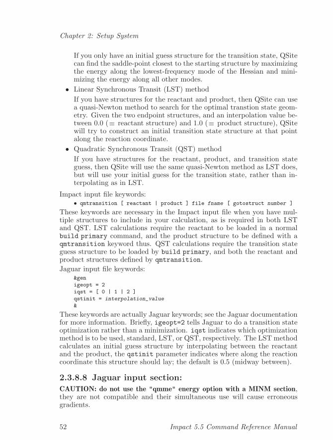
Chapter 2: Setup System
If you only have an initial guess structure for the transition state, QSitecan find the saddle-point closest to the starting structure by maximizingthe energy along the lowest-frequency mode of the Hessian and mini-mizing the energy along all other modes.
• Linear Synchronous Transit (LST) methodIf you have structures for the reactant and product, then QSite can usea quasi-Newton method to search for the optimal transtion state geom-etry. Given the two endpoint structures, and an interpolation value be-tween 0.0 (≡ reactant structure) and 1.0 (≡ product structure), QSitewill try to construct an initial transition state structure at that pointalong the reaction coordinate.
• Quadratic Synchronous Transit (QST) methodIf you have structures for the reactant, product, and transition stateguess, then QSite will use the same quasi-Newton method as LST does,but will use your initial guess for the transition state, rather than in-terpolating as in LST.
Impact input file keywords:• qmtransition [ reactant | product ] file fname [ gotostruct number ]
These keywords are necessary in the Impact input file when you have mul-tiple structures to include in your calculation, as is required in both LSTand QST. LST calculations require the reactant to be loaded in a normalbuild primary command, and the product structure to be defined with aqmtransition keyword thus. QST calculations require the transition stateguess structure to be loaded by build primary, and both the reactant andproduct structures defined by qmtransition.Jaguar input file keywords:
&gen
igeopt = 2
iqst = [ 0 | 1 | 2 ]
qstinit = interpolation_value
&
These keywords are actually Jaguar keywords; see the Jaguar documentationfor more information. Briefly, igeopt=2 tells Jaguar to do a transition stateoptimization rather than a minimization. iqst indicates which optimizationmethod is to be used, standard, LST, or QST, respectively. The LST methodcalculates an initial guess structure by interpolating between the reactantand the product, the qstinit parameter indicates where along the reactioncoordinate this structure should lay; the default is 0.5 (midway between).
2.3.8.8 Jaguar input section:
CAUTION: do not use the "qmme" energy option with a MINM section,they are not compatible and their simultaneous use will cause erroneousgradients.
52 Impact 5.5 Command Reference Manual
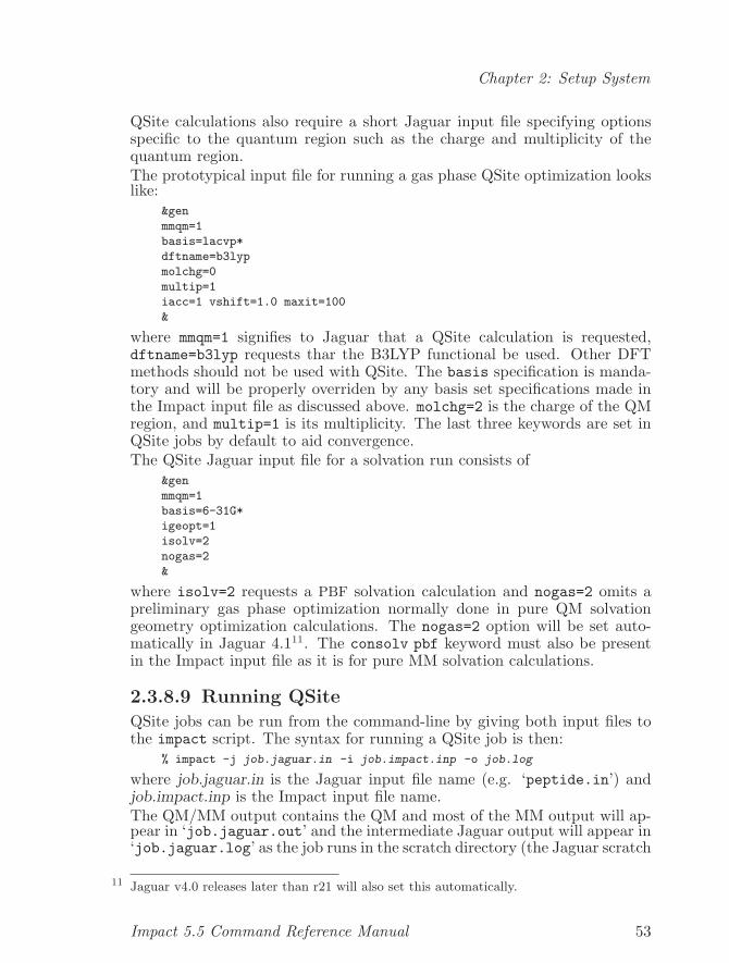
Chapter 2: Setup System
QSite calculations also require a short Jaguar input file specifying optionsspecific to the quantum region such as the charge and multiplicity of thequantum region.The prototypical input file for running a gas phase QSite optimization lookslike:
&gen
mmqm=1
basis=lacvp*
dftname=b3lyp
molchg=0
multip=1
iacc=1 vshift=1.0 maxit=100
&
where mmqm=1 signifies to Jaguar that a QSite calculation is requested,dftname=b3lyp requests thar the B3LYP functional be used. Other DFTmethods should not be used with QSite. The basis specification is manda-tory and will be properly overriden by any basis set specifications made inthe Impact input file as discussed above. molchg=2 is the charge of the QMregion, and multip=1 is its multiplicity. The last three keywords are set inQSite jobs by default to aid convergence.The QSite Jaguar input file for a solvation run consists of
&gen
mmqm=1
basis=6-31G*
igeopt=1
isolv=2
nogas=2
&
where isolv=2 requests a PBF solvation calculation and nogas=2 omits apreliminary gas phase optimization normally done in pure QM solvationgeometry optimization calculations. The nogas=2 option will be set auto-matically in Jaguar 4.111. The consolv pbf keyword must also be presentin the Impact input file as it is for pure MM solvation calculations.
2.3.8.9 Running QSite
QSite jobs can be run from the command-line by giving both input files tothe impact script. The syntax for running a QSite job is then:
% impact -j job.jaguar.in -i job.impact.inp -o job.log
where job.jaguar.in is the Jaguar input file name (e.g. ‘peptide.in’) andjob.impact.inp is the Impact input file name.The QM/MM output contains the QM and most of the MM output will ap-pear in ‘job.jaguar.out’ and the intermediate Jaguar output will appear in‘job.jaguar.log’ as the job runs in the scratch directory (the Jaguar scratch
11 Jaguar v4.0 releases later than r21 will also set this automatically.
Impact 5.5 Command Reference Manual 53
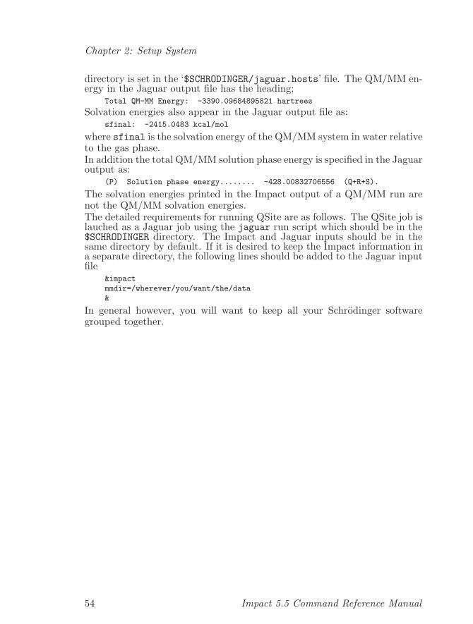
Chapter 2: Setup System
directory is set in the ‘$SCHRODINGER/jaguar.hosts’ file. The QM/MM en-ergy in the Jaguar output file has the heading;
Total QM-MM Energy: -3390.09684895821 hartrees
Solvation energies also appear in the Jaguar output file as:sfinal: -2415.0483 kcal/mol
where sfinal is the solvation energy of the QM/MM system in water relativeto the gas phase.In addition the total QM/MM solution phase energy is specified in the Jaguaroutput as:
(P) Solution phase energy........ -428.00832706556 (Q+R+S).
The solvation energies printed in the Impact output of a QM/MM run arenot the QM/MM solvation energies.The detailed requirements for running QSite are as follows. The QSite job islauched as a Jaguar job using the jaguar run script which should be in the$SCHRODINGER directory. The Impact and Jaguar inputs should be in thesame directory by default. If it is desired to keep the Impact information ina separate directory, the following lines should be added to the Jaguar inputfile
&impact
mmdir=/wherever/you/want/the/data
&
In general however, you will want to keep all your Schrodinger softwaregrouped together.
54 Impact 5.5 Command Reference Manual
Chapter 3: Perform Simulations
3 Perform Simulations
This chapter describes tasks that perform Impact simulations such as energyminimization and molecular dynamics, as well as linear response bindingaffinity calculations and ligand docking.
3.1 Task MinimizeMinimize a system using either the steepest descent or the conjugate gradientmethod. This task may only be called after the structural arrays have beenfilled and after a potential energy function has been set using setpotential.This task is used in many of the included examples.Results are printed every 10 steps by default, but this value can be adjustedvia the enrg parm print keywords in the SETMODEL task (see Section 2.3.1.6[Parm], page 25).Example:
minimize
read coordinates formatted file fname
steepest dx0 value dxm value deltae value
run
plot indiv quit
write coordinates formatted file fname
quit
3.1.1 Subtask SteepestUse the steepest descent algorithm for energy minimization of a system.
• steepest dx0 value dxm value
dx0 Initial step size (default = 0.05).dxm Maximum step size (default = 1.0).
3.1.2 Subtask ConjugateUse the conjugate gradient algorithm for energy minimization.
• conjugate dx0 value dxm value maxit number
dx0 step sizeSet the initial step size (default = 0.05).
dxm step sizeSet the maximum step size (default = 1.0).
maxit step sizeMaximum number of iterations for line search (default = 3).
rest Frequency of restarting with steepest descent (default =number of atoms ×3).
Impact 5.5 Command Reference Manual 55
Chapter 3: Perform Simulations
3.1.3 Subtask Tnewton
Use the truncated Newton algorithm (copyright (c) 1990 by Tamar Schlickand Aaron Fogelson, updated November 1998 by Dexuan Xie and TamarSchlick, used by permission)1 for energy minimization.PLEASE NOTE: This minimization algorithm cannot currently be used withperiodic boundary conditions, distance and torsional restraints and the FastMultipole Method.
• tnewton [nfull number] [nhscale number] -
[verbose number] [tncut value]
nfull Number of minimization steps per update of the long-rangeforces (as defined by the tncut value). The default is 10, andvalues higher than 20 are not recommended. Setting nfull toohigh can result in unrealistic structures and/or failure of theminimization. The short-range forces are updated at every min-imization step.
nhscale Scale factor for the size of the Hessian matrix. The amountof memory allocated for this matrix will be the nhscale valuetimes the number of atoms in the system. The default is 50.
verbose Controls the amount of printing. The default is 0. A positivevalue will result in a large amount of output, and is not recom-mended in general.
tncut Cutoff distance between short-range and long-range forces.Forces between atoms more distant than this will be calculatedonly every nfull minimization steps, as opposed to every stepfor the short-range forces. The default is 10.0 A.
3.1.4 Subtask InputThis subtask inputs parameters necessary for the minimizer.
• input cntl [ mxcyc num ] [ rmscut val ] [ deltae val ]
mxcyc The maximum number of cycles for the minimization (default= 100).
rmscut Criteria for convergence of the RMS gradient (default = 0.01).
deltae Criteria for convergence of the change in energy for each atom,average over the whole system (default = 1.0 · 10−7).
Important Notes:
1 For details, see Xie, D. and Schlick, T., “Remark on the Updated Truncated NewtonMinimization Package, Algorithm 702,” ACM Trans. Math Softw., 25, 108-122, March1999, and Xie, D. and Schlick, T., “Efficient implementation of the truncated-Newtonalgorithm for large-scale chemistry applications,” SIAM J. Opt., 10: 132-154, October1999.
56 Impact 5.5 Command Reference Manual
Chapter 3: Perform Simulations
1. The values for both rmscut and deltae must be met before a run isconverged.
2. The minimization will stop when the convergence criteria are met.
3.1.5 Subtask Run
This command signals the program to start running the minimization. Allother parameters must be set correctly before run is executed.
3.1.6 Subtasks Read and Write
Impact provides the write command to save to a file the molecular systemcoordinates in several formats. The write and read commands also offer asimple way of saving a snapshot of the system (coordinates and, if so desired,velocities) and restoring it afterwards.The following description applies not only to task minimize but also todynamics, and montecarlo, although in some cases (to be discussed below)not all options would make sense. There are three types of file that can beused to hold snapshots of the system: PDB (brookhaven or impact format),Maestro, residue template, restart and trajectory files.To write a PDB file use the following syntax:
• write pdb [ brookhaven | impact | nil ] -
name species_name file filename
Note: only coordinates can be written to a PDB file. To read a PDB fileyou must do so inside the create task.To write a Maestro file use the following syntax:
• write maestro [ name spec1 [ name spec2] ] -
file filename
If the species to be written to the Maestro file are of type ‘auto’ the infor-mation from the original Maestro file (or as converted from a PDB or SD file)is preserved in the output of this command. If the species is of type otherthan ‘auto’, Impact attempts to generate a valid Maestro file by creating atype ‘auto’ temporary copy of the species before writing it to the file. If twospecies are specified, a temporary species of type ‘auto’ obtained by mergingthe two species is written to the file. In absence of species specification thedefault is to merge both Impact species in the output file. To read a Maestrofile you must do so inside the create task.The write restart and read restart commands are used to save and re-store the coordinates (and velocities) of all particles in the system. A restartfile consists of a snapshot of the cartesian coordinates and, optionally, ve-locities of each atom of the system. When reading or writing restart filesthe behavior of Impact depends on the current task unless the files are writ-ten and read using the external keyword, in which case Impact honors allrequests made on the command line.
Impact 5.5 Command Reference Manual 57
Chapter 3: Perform Simulations
• In task minimize only coordinates can be written or read. If the com-mand line also specifies velocities Impact will not honor the requestunless external format is used, although no error will be generated.
• In task montecarlo only coordinates can be written but both coordi-nates and velocities can be read.2
• In task dynamics velocities are always written to a restart file, even ifthey are not specified on the command line. The user can, however,choose not to read them back.
In all cases the usage is the same:• [ read | write ] restart coordinates [ and velocities ]
[ box | nobox | nil ] -
[ formatted | unformatted | external | nil ] -
[ real8 | real4 | inte2 | nil ] -
file filename
The meaning of the keywords is explained below.A trajectory file contains a sequence of snapshots of the system (coordinatesand, sometimes, velocities of all atoms). Normally trajectory files are readusing the table subtasks starttrack and stoptrack but they can also beread wherever a restart file can be read.
• write trajectory coordinates [ and velocities ] [ box | nobox | nil ] -
[ unformatted | external | nil ] -
[ real8 | real4 | inte2 | nil ] -
file filename -
every number_of_steps
• read restart coordinates [ and velocities ] [ box | nobox | nil ] -
[ unformatted | external | nil ] -
[ real8 | real4 | inte2 | nil ] -
file filename -
skip to frame_number
Caution: reading a frame (snapshot) from a trajectory file using the lastsyntax shown should be done with care, since strange things may happen ifthe user mixes the coordinates with the velocities.
formattedunformattedexternal (default for restart and trajectory files) A formatted file is an
ASCII file containing the list of coordinates (and velocities, ifappropriate). The main advantage of these files is that theyare human readable, but they usually occupy too much space.An unformatted file, on the other hand, is binary and thusmuch smaller. The main disadvantage is that files generatedon one machine are usually not readily read on other machines.This prompted the development of the external way of writing
2 Though velocities are not very meaningful in this case.
58 Impact 5.5 Command Reference Manual
Chapter 3: Perform Simulations
restart and trajectory files, which offers a compact (since it is bi-nary), machine-independent representation. This is the defaultfor trajectory files and it is strongly recommended (unformattedfiles may not be supported in the future). As mentioned above,if the keyword external is specified Impact honors all requestson the command line.
inte2real4
real8 (default)These keywords control the size of the data written to (readfrom) a binary restart or trajectory file. When reading anunformatted file they must be specified, but that is not neces-sary when reading an external file since the program can findthis information from the file itself. The keyword inte2 will beignored when reading or writing an external file and real4 willbe substituted instead. The sizes are chosen as follows:
real8 Store the data as real*8 numbers. This is the high-est precision available and uses the most disk space.
real4 Stores the data as real*4 numbers. This halves thestorage requirements and also reduces the precision.
inte2 This option is somewhat more complicated. Thenumbers will be scaled by 1000. and stored asinteger*2 numbers. This will leave a maximumof 5 significant figures and maximum values of±32.767.
[ box | nobox | nil ]Write (or don’t write) the dimensions of the simulation volumewith the coordinates (these dimensions are needed when per-forming constant pressure simulations). If a constant pressuresimulation is being run, box is the default; otherwise it is nobox.This option applies to trajectory and restart files.
every number of stepsDetermines how often coordinate sets will be written.
skip to frame numberWhen reading a trajectory as a restart file one can specify whichframe (snapshot) to read. Frame numbers start at 1 and shouldnot exceed the number of frames that were written to the file.
Impact 5.5 Command Reference Manual 59

Chapter 3: Perform Simulations
3.2 Task DynamicsThe object of task dynamics is to perform a molecular dynamics (MD)simulation for a system prepared by tasks create and setmodel.Please Note: Dynamics simulations may not give useful results, or may ter-minate with errors, if the initial structure has steric clashes or other prob-lems. Even structures that have been minimized with other programs, orthose produced by Maestro’s build panel, may have such problems as mea-sured with Impact’s force fields. A short Impact minimization task prior todynamics is useful for fixing such problems.
3.2.1 Subtask Input
Reads in program control parameters for the MD run.• input cntl nstep steps [ delt time_step ]
• input cntl [ constant -
[ temperature [ byspecies ] [ relax value ] | totalenergy ] -
[ pressure [ dvdp value ] [ density value ] | volume ]
• input cntl [ initialize temperature -
[ forspecies ( name spec at T_i ) for all species | -
at T_i ] [ seed num ] ] -
[ stop rotations ] [ nprnt freq) ] -
[ tol tolerance ] [metric value]
• input cntl [ statistics [ on | off ] ]
Unless otherwise specified the default is to run MD simulations at con-stant temperature and volume. This results in coupling the system toan external heat bath (with a temperature that is independent of thespecies). Using the keyword byspecies results in velocity scalings thatare independent for each species. In this case the user should specifyan initial temperature for each species using the forspecies keyword,and all species should appear on the same (logical) line. Otherwisesome of the species will end up with the default initial temperature. If‘constant totalenergy’ is specified instead there will be no scaling.1
Specifying ‘constant pressure’, as opposed to ‘constant volume’, re-sults in coupling to a pressure bath using the algorithm of Berendsen etal. (J. Chem. Phys., 81, 3684 (1984)). Molecular center of mass coordi-nate rescaling is implemented. The distances between molecules changeproportionally to the change in box size and intramolecular distances re-main unchanged. Note that a "molecule" is defined as the entity createdby a ‘build primary’ command. Center of mass coordinate rescaling isineffective for systems composed of a single molecule (systems built withonly one ‘build primary’ command). A solvent species is composed ofas many molecules as created by the ‘build solvent’ command.
1 The total energy may actually not be conserved, due to the effects of a sharp cutoff. Inmost cases this will lead to an unstable simulation.
60 Impact 5.5 Command Reference Manual
Chapter 3: Perform Simulations
Independent of whether the simulation is run at ‘constanttemperature’ or ‘constant totalenergy’ the user can initialize thetemperature of all species (either the same for all or on a per-speciesbasis) with the keywords ‘initialize temperature’. Caution: bydefault the temperature is not initialized since this could result inoverwriting the velocities read from a restart file. Right after aminimization, the user should initialize the temperatures of all speciesto sensible values. The user should not use ‘initialize temperature’though, if there is an external restart file (with both coordinates andvelocities) read in.Several parameters can be specified in the ‘input cntl’ line:
nstep Number of MD steps (must be larger than one!).
nprnt Gives the number of steps after which contributions to theenergy will be printed out (5).
delt Gives the time step in picoseconds (0.001).
relax Relaxation time in ps for velocity scaling (if using ‘constanttemperature’) (0.01).
seed Seed to be used to start the random number generator wheninitializing the temperature of (any) species.
taup Relaxation time in ps for volume scaling (if using ‘constantpressure’) (0.01).
dvdp Isothermal compressibility 1/V (dV/dP ), in units of atm−1.The default is the value for water: 4.96 · 10−5 atm−1. Thisquantity is needed for constant pressure simulations.
density Effective density (g/cm3) of solute molecules. Needed tocompute long-range corrections to the pressure (1.0).
tol Tolerance to be used when applying the constraints in SHAKEand RATTLE (1.0 · 10−7).
stop rotationsFlag for stopping the center of mass motion. Default is notto stop the center of mass motion.
statistics onstatistics off
Toggles collection of statistics on the fluctuations of thedifferent energy terms during the simulation. In earlier ver-sions this was always on; now it is off by default.
• input target temperature T_f
• input target ( [ name spec ] temperature T_f ) repeated for all species
Allows the specification of the final temperature (T f ) for the wholesystem or by species. The first form should be used only if the scaling
Impact 5.5 Command Reference Manual 61
Chapter 3: Perform Simulations
is done on a species-independent basis. If the byspecies keyword wasused, however, the second form must be used and all the species shouldappear on the same (logical) line. Multiple ‘input target’ lines wouldresult in conflicts.The actual temperature will fluctuate about the desired value. At eachMD step the kinetic energies will be scaled so the temperature willapproach the desired value on a timescale determined by the relaxparameter.• input target pressure P_f
Reads in the final pressure (P f ) of the system. The same comment asin the previous paragraph applies, mutatis mutandis.
3.2.2 Subtask Run
Performs the actual molecular dynamics run. The temperatures are initial-ized at this step, not when the values are read from the ‘input cntl’ line.The user can choose among three different algorithms for the integration ofthe equations of motion: the Verlet algorithm, which is the default; and twobased on the reversible RESPA (r-RESPA) of Tuckerman, Berne and Mar-tyna, J. Chem. Phys., 97 (1992). Currently at most three inner stages areallowed and the frequency with which the corresponding forces are updatedis controlled by the parameters freqf (fast forces), freqm (medium and slowforces) and freqs (slow forces). Currently freqm and freqs only have meaningif the FMM (fast multipole) code is used. On the other hand, freqf can beused with or without the FMM since it controls only the bonding forces.If the FMM is used and freqs is present, the forces are separated in threepieces: those arising from nearby bodies; those arising from bodies in thefirst and second neighbors that are not very close, and those coming fromthe local expansions. If freqs is not present but freqm is, the second andthird are collected together.
• run [ verlet | rrespa fast freqf [ medium freqm [ slow freqs ] ] ]
3.2.3 Subtasks Read and Write
Read or Write a) a restart file containing final coordinates, and velocities(forces could also be written) or b) a trajectory file (see Section 3.1.6[Read/write (minimize)], page 57).
3.2.4 Subtask Convert
This subtask is provided to ease the transition to the new, default, externalbinary format (see Section 3.1.6 [Read/write (minimize)], page 57).
• convert -
from [ unformatted | external ] file filename -
to [ unformatted | external ] file filename -
[ real4 | real8 | inte2 ] [ box | nobox ] -
[ first start last end ]
62 Impact 5.5 Command Reference Manual
Chapter 3: Perform Simulations
Reads a trajectory file written in one format and writes it out in an-other. The keywords box, nobox, real8, real4 and inte2 apply onlyto the output file and allow the user to specify the corresponding op-tions differently from the ones used when the input file was written (seeSection 3.1.6 [Read/write (minimize)], page 57). Note that inte2 is thesame as real4 when using the external format.The parameters start and end allow the user to convert only a portionof the trajectory file. Since both input and output formats can be thesame this is a handy way of extracting a consecutive sequence of frames.
Impact 5.5 Command Reference Manual 63
Chapter 3: Perform Simulations
3.3 Task Hybrid Monte Carlo (HMC)The Hybrid Monte Carlo (HMC) method is often called “bad MD but goodMC”. Even though HMC is regarded as a Monte Carlo method, it usesMolecular Dynamics to perform the conformation-space search. Thus, inmany respects, HMC’s subtasks can be compared to those for MolecularDynamics, as both usually call the same functions. Since molecular dynamicsis only used for generating new conformations, a much larger time stepcan usually be used (this is why it is called bad MD), with the Metropoliscriterion determining which moves to accept or reject.
3.3.1 HMC Methodology
The J-Walking and S-Walking methods are also implemented on the basisof the HMC protocol, and can be turned on by specifying subtasks. SinceHMC performs the same simulation as does constant temperature moleculardynamics, many input controls for constant temperature MD are also suit-able for HMC or are very similar for it, as you can see from the exampleshown below.
The following is a brief description of the S-walking (Smart Walking) methodproposed by R. Zhou and B. J. Berne.1 The S-Walking method is closely re-lated to the J-Walking method proposed by Frantz et al.2 Like the J-Walkingmethod, the S-Walking method runs two walkers, one at the temperature ofinterest, the other at a higher temperature that more efficiently generatesergodic distributions. Instead of sampling from the Boltzmann distributionof the higher temperature walker as in J-Walking, S-Walking first approx-imately minimizes the structures being jumped into, and then uses the re-laxed structures as the trial moves at the low temperature. By jumping intoa relaxed structure, or a local minimum, the jump acceptance ratio increasesdramatically. This makes the protein system easily undergo barrier-crossingevents from one basin to another, thus greatly improving the ergodicity ofthe sampling. The method approximately preserves detailed balance pro-vided the time between jumps is large enough to allow effective sampling ofconformations in each local basin.
Here is a very simple example of a HMC calculation that uses S-Walking
1 J. Chem. Phys., 107, 9185 (1997)2 J. Chem. Phys. 93, 2769 (1990)
64 Impact 5.5 Command Reference Manual
Chapter 3: Perform Simulations
HMC
input cntl mxcyc 10000 nmdmc 5 delt 0.0015 relax 0.01 seed 101 -
nprnt 100 tol 2.0e-7
input cntl swalk cycgap 5000 cycrec 20 minstep 100 -
jtemp 500.0 jrate 0.1
input target temperature 300.0
write trajectory coordinates and velocities every 10 -
external file pentpep.trj
run
write restart coordinates and velocities formatted file pentpep.rst
write pdb brookhaven name pentpep file pentpep_swk.pdb
QUIT
3.3.2 Subtask Input
Reads in program control parameters for the HMC run.• input cntl mxcyc cycles [ nmdmc num ] [delt time_step ] -
[ relax val] [ seed num ] [ stop rotations ] [ nprnt freq ] -
[ tol tol ] [metric value]
• input cntl [ statistics [ on | off ] ]
• input cntl [ swalk | jwalk ] [ cycgap cycles ] [cycrec cycles ] -
[ jtemp temp ] [ jrate rate ] [ minstep steps ] [metric num ]
• input target temperature T_f
HMC samples the conformation space with the canonical ensemble.Thus the underlying molecular dynamics by default is constant tem-perature constant volume MD. This results in coupling the system toan external heat bath with a temperature that is specified by ‘targettemperature’. Note that unlike dynamics, there is no ‘initializetemperature’ option for HMC. Instead, HMC initializes velocities to adistribution based on ‘target temperature’ at the beginning of eachHMC step.Several parameters can be specified in the ‘input cntl’ line:
mxcyc Number of HMC cycles to be performed.
nmdmc Number of MD steps per HMC cycle (5). The total numberof MD steps will be equal to (mxcyc * nmdmc).
nprnt Number of MD steps after which contributions to the energywill be printed out (5).
delt Time step in picoseconds (0.001).
relax Relaxation time in ps for velocity scaling (if using ‘constanttemperature’) (0.01).
seed Seed to be used to start the random number generator wheninitializing the velocities for any species.
tol Tolerance to be used when applying the constraints in SHAKEand RATTLE (1.0 · 10−7).
Impact 5.5 Command Reference Manual 65
Chapter 3: Perform Simulations
jwalk Turn on the jwalk option. This option performs J-Walkingwith other parameters specified by following items. It runsan extra high-temperature walker for barrier crossing, sothe total MD steps will be doubled.
swalk Turn on the swalk option. This option performs S-Walkingwith other parameters specified by following items. It alsoruns an extra high-temperature walker for barrier crossing,so the total MD steps will be doubled. The difference be-tween swalk and jwalk is that swalk option performs arough local minimization for high-temperature conforma-tions, while the jwalk option does not.
cycgap Number of HMC cycles for the high-temperature walker orlow-temperature walker before they switch (1000). The twowalkers are run in tandem.
cycrec Number of HMC cycles between records written of thehigh temperature-walker’s configuration (20), where cyc-gap/cycrec = number of records stored in file highT.cnf.
jrate Trial jump rate (1.0%).
jtemp Jump-S/Jwalker’s (high-temperature walker) temperature(500.0 K).
minstep Steepest decent minimization steps in S-walking (100)
metric Parameter for ergodicity analysis (0). metric = 1, performergodic metric calculation; metric = 0, no metric calcula-tion.
stop rotationsFlag for stopping the center of mass motion. Default is notto stop the center of mass motion.
statistics onstatistics off
Toggles collection of statistics on the fluctuations of thedifferent energy terms during the simulation. In earlier ver-sions this was always on; now it is off by default.
• input target temperature T_f
Allows the specification of the final temperature (T f ) for the wholesystem. The actual temperature will fluctuate about the desired value.At each MD step the kinetic energies will be scaled so the temperaturewill approach the desired value on a timescale determined by the relaxparameter.
66 Impact 5.5 Command Reference Manual
Chapter 3: Perform Simulations
3.3.3 Subtask Run
Performs the actual molecular dynamics run, as described in the MolecularDynamics Run subection (see Section 3.2.2 [Run (dynamics)], page 62). Thetemperatures are initialized at this step, not when the values are read fromthe ‘input cntl’ line. The user can choose among three different algorithmsfor the integration of the equations of motion: the Verlet algorithm, whichis the default; and two based on the reversible RESPA (r-RESPA) of Tuck-erman, Berne and Martyna, J. Chem. Phys., 97 (1992). Currently at mostthree inner stages are allowed and the frequency with which the correspond-ing forces are updated is controlled by the parameters freqf (fast forces),freqm (medium and slow forces) and freqs (slow forces). Currently freqmand freqs only have meaning if the FMM (fast multipole) code is used. Onthe other hand, freqf can be used with or without the FMM since it controlsonly the bonding forces. If the FMM is used and freqs is present, the forcesare separated in three pieces: those arising from nearby bodies; those arisingfrom bodies in the first and second neighbors that are not very close, andthose coming from the local expansions. If freqs is not present but freqm is,the second and third are collected together.
• run [ verlet | rrespa fast freqf [ medium freqm [ slow freqs ] ] ]
3.3.4 Subtasks Read and Write
Read or Write a) a restart file containing final coordinates, and velocities(forces could also be written) or b) a trajectory file (see Section 3.1.6[Read/write (minimize)], page 57).
3.3.5 Subtask Convert
This subtask is provided to ease the transition to the new, default, externalbinary format (see Section 3.1.6 [Read/write (minimize)], page 57).
• convert -
from [ unformatted | external ] file filename -
to [ unformatted | external ] file filename -
[ real4 | real8 | inte2 ] [ box | nobox ] -
[ first start last end ]
Reads a trajectory file written in one format and writes it out in an-other. The keywords box, nobox, real8, real4 and inte2 apply onlyto the output file and allow the user to specify the corresponding op-tions differently from the ones used when the input file was written (seeSection 3.1.6 [Read/write (minimize)], page 57). Note that inte2 is thesame as real4 when using the external format.The parameters start and end allow the user to convert only a portionof the trajectory file. Since both input and output formats can be thesame this is a handy way of extracting a consecutive sequence of frames.
Impact 5.5 Command Reference Manual 67
Chapter 3: Perform Simulations
3.4 Task Linear Response Method (Liaison, LRM,or LIA)
Liaison, embodied in the LRM or LIA task, is Schrodinger’s implementation ofthe Linear Response Method (LRM), also called the Linear Interaction Ap-proximation (LIA), a method of combining molecular mechanics calculationswith experimental data to build a model scoring function for the evaluationof ligand-protein binding free energies.
3.4.1 Liaison Overview
LRM-type methods were first suggested by Aqvist (J. Aqvist, C. Medinaand J. EA. Samuelsson, Protein Eng. 7, 385-391, 1994; T. Hansson and J.Aqvist, Protein Eng. 8, 1137-1144, 1995), based upon approximating thecharging integral in the free energy perturbation formula with a mean valueapproach in which the integral is represented as half the sum of the valuesat the endpoints, namely the free and bound states of the ligand. Since thenthey have been pursued by a number of research groups including that ofJorgensen (D. K. Jones-Hertzog and W. L. Jorgensen, J. Med. Chem., 40,1539-1549, 1997), who has reported very good results for a number of ligandbinding data sets. From a computational standpoint, this approximationhas a number of highly attractive features:
1. In contrast to free energy perturbation (FEP), where a large number ofintermediate windows must be evaluated, the LIA requires simulationsof only the ligand in solution and the ligand bound to the protein. Theidea is that one views the binding event as a replacement of the aqueousenvironment of the ligand with a mixed aqueous/protein environment.
2. Again in contrast to FEP, one can study disparate ligands as long asthey have similar binding modes. FEP allows only very small changesbetween ligands to be investigated; the differences in the data sets wehave examined up to this point are much more significant.
3. Only interactions between the ligand and either the protein or the aque-ous environment enter into the quantities that are accumulated duringthe simulation; the ligand-ligand, protein-protein and protein-water in-teractions are part of the “reference” Hamiltonian and hence are usedto generate configurations in the simulation (via either Monte Carlo ormolecular dynamics) but are not used as descriptors in the resultingmodel for the binding free energy (see below). This eliminates a consid-erable amount of noise and systematic uncertainties in the calculations,for example arising from different conformations of the protein obtainedfrom cocrystallized structures of different ligands.
4. The method as implemented by Jorgensen et al. contains three termsin the empirical formula for the binding energy: electrostatic, van derWaals, and solvent accesible surface area (SASA):
68 Impact 5.5 Command Reference Manual
Chapter 3: Perform Simulations
∆G = α(〈U belec〉 − 〈U f
elec〉) + β(〈U bvdw〉 − 〈U f
vdw〉) + γ(〈U bSASA〉 − 〈U f
SASA〉)
〈...〉means ensemble average from a Monte Carlo or Molecular Dynamicssimulation, and all terms are evaluated only for interactions betweenligand and its “environment”. Aqvist et al. used only two terms intheir original work, i.e., electrostatic and van der Waals interaction.However, Jorgensen et al. found that it is necessary to add one moreterm for larger data sets, and the third term was also proposed to bejust a constant term. In our implementation as discussed later, the thirdterm is based on the cavity energy in the SGB continuum solvent model.
If the linear response approximation was rigorously valid, the coefficientof the electrostatic term would be 0.5, corresponding to the mean valueapproximation to the charging integral. In fact, one can recover a value veryclose to this for less complex systems, such as solvation of small molecules inwater. However, some of the steps involved in the binding event, such as theremoval of water from the protein cavity and subsequent introduction of theligand, are unlikely to be accurately described by a linear model. Therefore,in practice, optimization of fitting parameters yields electrostatic coefficientsthat are significantly different from the ideal value of 0.5. By allowing thisempirical element, one is sacrificing generality; the method probably requiresthat the ligands have similar binding modes, and new parameters must bedeveloped for each receptor. In return, however, one can obtain a reasonablelevel of accuracy (reflected in cross-validation studies as well as the overallfitting accuracy) with a modest expenditure of CPU time, under assumptionsthat are quite reasonable for many structure-based drug design projects.We have developed an implementation of the LIA, in the context of theImpact program, using the generalized Born continuum solvation model andthe OPLS-AA force field of Jorgensen and coworkers. To our knowledge, thisis the first commercially available version of the LIA and the first versionof any type to utilize continuum solvation. Key features of the Schrodingerimplementation are as follows:1. First, we replaced the solvent accessible surface area term in Jorgensen’s
LIA formulation by the cavity term in the continuum solvent model:
∆G = α(〈U belec〉 − 〈U f
elec〉) + β(〈U bvdw〉 − 〈U f
vdw〉) + γ(〈U bcav〉 − 〈U f
cav〉).
We think it makes sense to use such a term in the context of a continuumsolvent model. Indeed, it is not clear why the solvent accessible surfacearea is needed in an explicit solvent model, since waters are explicitlyrepresented already.
Impact 5.5 Command Reference Manual 69
Chapter 3: Perform Simulations
2. The use of a continuum model provides much more rapid convergenceof the simulations. The statistics on the various interaction terms aresignificantly better converged than in an explicit solvent simulation, andthe required CPU time is much smaller.
3. We have implemented an automatic atom typing scheme for the OPLS-AA force field that assigns charges, van der Waals, and valence parame-ters with no human intervention. A key feature of OPLS-AA is excellentreproduction of condensed phase properties, obtained via fitting to liq-uid state simulations. Over the past years Jorgensen and coworkers haverapidly extended the functional-group coverage of OPLS-AA to includea larger number of pharmaceutically relevant species. This work willbe continued and expanded at Schrodinger and at Columbia University(Prof. Richard Friesner) in collaboration with Professor Jorgensen. Weintend in the coming year to increase both the accuracy and coverageof OPLS-AA substantially.
4. The Maestro interface to Liaison produces scripts that allow a series ofLiaison jobs to be run automatically. This makes it convenient to usethe method in the context of an industrial structure-based drug designeffort, in which a large number of molecules need to be examined.
Here is a very simple LRM example that uses the SGB continuum solventmodel
LRM
assign ligand name drug
input cntl average every 10 file lrm_bound.ave
sample dynamics
input cntl nstep 10000 delt 0.001 relax 0.01 nprnt 100 seed 101 -
constant temperature
input target temperature 300.0
run rrespa fast 2
write restart coordinates and velocities formatted file cmpx_lrm.rst
write pdb brookhaven name prot file prot_lrm.pdb
write pdb brookhaven name drug file lig_lrm.pdb
QUIT
3.4.2 Subtask Assign
Specifies the LRM or LIA ligand in the LRM simulation. This ligand canin fact be any entity; it could be a single ligand, a pair of ligands from aternary complex, or even a protein, as long as all the components reside ina single species.
• assign ligand name spec
name spec determines the LRM ligand. The program thus will calculate andcollect all interactions between this ligand and its “environment” (proteinor water), but not the interactions within ligand itself or the protein (water)itself. In the continuum solvent model, this means that we need to separate
70 Impact 5.5 Command Reference Manual
Chapter 3: Perform Simulations
the single and pairwise energies in the Generalized Born model into properpartial contributions to represent the LIA interaction between ligand andprotein.
3.4.3 Subtask Param
Specifies LRM or LIA parameters, i.e., α, β, γ in the LRM simulation.
• param elec val vdw val cavity val
As mentioned above, the current method requires that new parameters bedeveloped for each receptor, so this option is not actually used at present.Schrodinger’s Maestro user interface generates scripts, as described below,that automate the LRM simulations on various ligands with known bindingenergies, and perform the requisite data collection. Then the user can runanother script to calculate the LRM parameters and report the goodnessof the fit to the experimental binding energies. Finally, the user can applythese parameters to predict the binding energies of new systems.
3.4.4 Subtask Input
Reads in program control parameters for the LRM simulation.
• input cntl average every num file filename
This command controls options for collection of the LRM statistics. It speci-fies how often the average LRM interaction energies are to be calculated andwhich file to use to print out the ensemble averages. (Other LRM-specificoptions may also be specifiable here in the future.)
every Calculate the LRM ensemble average every num steps.
file Write out the ensemble averages to file filename.
3.4.5 Subtask Sample
Selects a sampling method for the LRM simulation, such as Molecular Dy-namics or Hybrid Monte Carlo.
• sample [ dynamics | HMC ]
The commands that follow the choice of sampling method are identical tothose that would be needed if that method were invoked as a standalone task.This is illustrated in the previous example, where dynamics was chosen asthe sampling method; all commands after dynamics are identical to thoseexpected for the dynamics task. The following example uses HMC as thesampling method:
Impact 5.5 Command Reference Manual 71
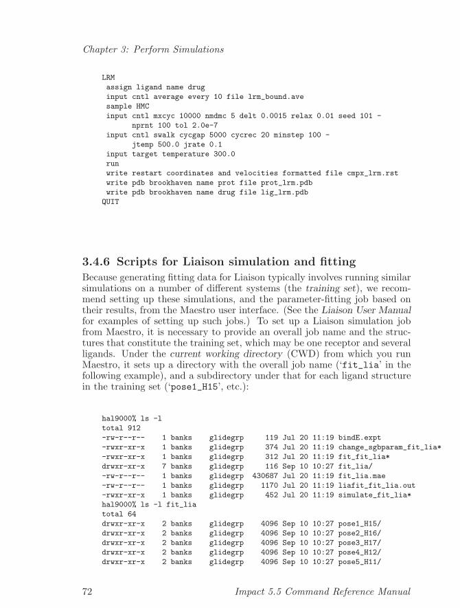
Chapter 3: Perform Simulations
LRM
assign ligand name drug
input cntl average every 10 file lrm_bound.ave
sample HMC
input cntl mxcyc 10000 nmdmc 5 delt 0.0015 relax 0.01 seed 101 -
nprnt 100 tol 2.0e-7
input cntl swalk cycgap 5000 cycrec 20 minstep 100 -
jtemp 500.0 jrate 0.1
input target temperature 300.0
run
write restart coordinates and velocities formatted file cmpx_lrm.rst
write pdb brookhaven name prot file prot_lrm.pdb
write pdb brookhaven name drug file lig_lrm.pdb
QUIT
3.4.6 Scripts for Liaison simulation and fitting
Because generating fitting data for Liaison typically involves running similarsimulations on a number of different systems (the training set), we recom-mend setting up these simulations, and the parameter-fitting job based ontheir results, from the Maestro user interface. (See the Liaison User Manualfor examples of setting up such jobs.) To set up a Liaison simulation jobfrom Maestro, it is necessary to provide an overall job name and the struc-tures that constitute the training set, which may be one receptor and severalligands. Under the current working directory (CWD) from which you runMaestro, it sets up a directory with the overall job name (‘fit_lia’ in thefollowing example), and a subdirectory under that for each ligand structurein the training set (‘pose1_H15’, etc.):
hal9000% ls -l
total 912
-rw-r--r-- 1 banks glidegrp 119 Jul 20 11:19 bindE.expt
-rwxr-xr-x 1 banks glidegrp 374 Jul 20 11:19 change_sgbparam_fit_lia*
-rwxr-xr-x 1 banks glidegrp 312 Jul 20 11:19 fit_fit_lia*
drwxr-xr-x 7 banks glidegrp 116 Sep 10 10:27 fit_lia/
-rw-r--r-- 1 banks glidegrp 430687 Jul 20 11:19 fit_lia.mae
-rw-r--r-- 1 banks glidegrp 1170 Jul 20 11:19 liafit_fit_lia.out
-rwxr-xr-x 1 banks glidegrp 452 Jul 20 11:19 simulate_fit_lia*
hal9000% ls -l fit_lia
total 64
drwxr-xr-x 2 banks glidegrp 4096 Sep 10 10:27 pose1_H15/
drwxr-xr-x 2 banks glidegrp 4096 Sep 10 10:27 pose2_H16/
drwxr-xr-x 2 banks glidegrp 4096 Sep 10 10:27 pose3_H17/
drwxr-xr-x 2 banks glidegrp 4096 Sep 10 10:27 pose4_H12/
drwxr-xr-x 2 banks glidegrp 4096 Sep 10 10:27 pose5_H11/
72 Impact 5.5 Command Reference Manual
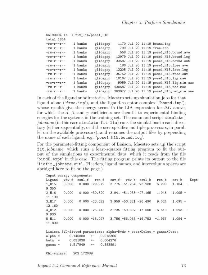
Chapter 3: Perform Simulations
hal9000% ls -l fit_lia/pose1_H15
total 1864
-rw-r--r-- 1 banks glidegrp 1170 Jul 20 11:19 bound.inp
-rw-r--r-- 1 banks glidegrp 799 Jul 20 11:19 free.inp
-rw-r--r-- 1 banks glidegrp 558 Jul 20 11:19 pose1_H15.bound.ave
-rw-r--r-- 1 banks glidegrp 12979 Jul 20 11:19 pose1_H15.bound.log
-rw-r--r-- 1 banks glidegrp 33587 Jul 20 11:19 pose1_H15.bound.out
-rw-r--r-- 1 banks glidegrp 186 Jul 20 11:19 pose1_H15.free.ave
-rw-r--r-- 1 banks glidegrp 12205 Jul 20 11:19 pose1_H15.free.log
-rw-r--r-- 1 banks glidegrp 35752 Jul 20 11:19 pose1_H15.free.out
-rw-r--r-- 1 banks glidegrp 10167 Jul 20 11:19 pose1_H15_lig.mae
-rw-r--r-- 1 banks glidegrp 9059 Jul 20 11:19 pose1_H15_lig_min.mae
-rw-r--r-- 1 banks glidegrp 430687 Jul 20 11:19 pose1_H15_rec.mae
-rw-r--r-- 1 banks glidegrp 363077 Jul 20 11:19 pose1_H15_rec_min.mae
In each of the ligand subdirectories, Maestro sets up simulation jobs for thatligand alone (‘free.inp’), and the ligand-receptor complex (‘bound.inp’),whose results give the energy terms in the LIA expression for ∆G above,for which the α, β, and γ coefficients are then fit to experimental bindingenergies for the systems in the training set. The command script simulate_jobname (in this case simulate_fit_lia) runs the simulations in each direc-tory (either sequentially, or if the user specifies multiple processors, in paral-lel on the available processors), and renames the output files by prependingthe name of each ligand, e.g. ‘pose1_H15.bound.log’.For the parameter-fitting component of Liaison, Maestro sets up the scriptfit_jobname, which runs a least-squares fitting program to fit the out-put of the simulations to experimental data, which it reads from the file‘bindE.expt’ in this case. The fitting program prints its output to the file‘liafit_jobname.out’. (Headers, ligand names, and intercolumn spaces areabridged here to fit on the page.)
Input energy components:
Ligand vdw_f coul_f rxn_f cav_f vdw_b coul_b rxn_b cav_b Expt
1_H15 0.000 0.000 -29.979 3.775 -51.264 -23.280 6.290 1.104 -
9.350
2_H16 0.000 0.000 -30.520 3.941 -51.035 -27.165 1.046 1.095 -
11.190
3_H17 0.000 0.000 -23.622 3.959 -56.821 -26.490 9.024 1.095 -
12.160
4_H12 0.000 0.000 -25.415 3.735 -50.892 -17.000 -6.610 1.093 -
9.930
5_H11 0.000 0.000 -18.047 3.756 -56.033 -16.753 -1.967 1.094 -
11.890
Liaison SVD-fitted parameters: alpha*Dvdw + beta*Delec + gamma*Dcav:
alpha = 0.145880 +- 0.018366
beta = 0.031038 +- 0.004276
gamma = 1.517949 +- 0.383891
Chi-square: 202.172089
Impact 5.5 Command Reference Manual 73
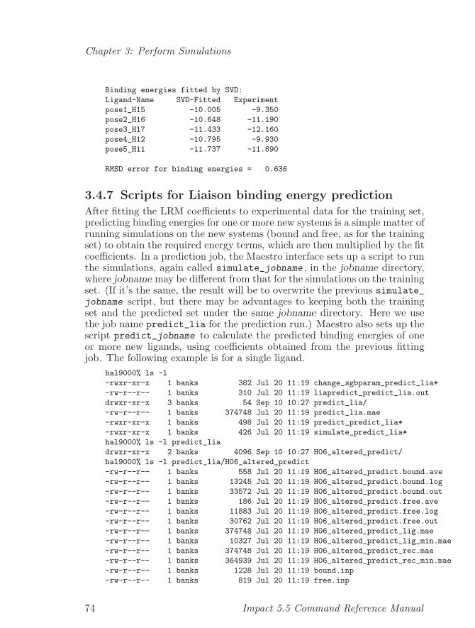
Chapter 3: Perform Simulations
Binding energies fitted by SVD:
Ligand-Name SVD-Fitted Experiment
pose1_H15 -10.005 -9.350
pose2_H16 -10.648 -11.190
pose3_H17 -11.433 -12.160
pose4_H12 -10.795 -9.930
pose5_H11 -11.737 -11.890
RMSD error for binding energies = 0.636
3.4.7 Scripts for Liaison binding energy prediction
After fitting the LRM coefficients to experimental data for the training set,predicting binding energies for one or more new systems is a simple matter ofrunning simulations on the new systems (bound and free, as for the trainingset) to obtain the required energy terms, which are then multiplied by the fitcoefficients. In a prediction job, the Maestro interface sets up a script to runthe simulations, again called simulate_jobname , in the jobname directory,where jobname may be different from that for the simulations on the trainingset. (If it’s the same, the result will be to overwrite the previous simulate_jobname script, but there may be advantages to keeping both the trainingset and the predicted set under the same jobname directory. Here we usethe job name predict_lia for the prediction run.) Maestro also sets up thescript predict_jobname to calculate the predicted binding energies of oneor more new ligands, using coefficients obtained from the previous fittingjob. The following example is for a single ligand.
hal9000% ls -l
-rwxr-xr-x 1 banks 382 Jul 20 11:19 change_sgbparam_predict_lia*
-rw-r--r-- 1 banks 310 Jul 20 11:19 liapredict_predict_lia.out
drwxr-xr-x 3 banks 54 Sep 10 10:27 predict_lia/
-rw-r--r-- 1 banks 374748 Jul 20 11:19 predict_lia.mae
-rwxr-xr-x 1 banks 498 Jul 20 11:19 predict_predict_lia*
-rwxr-xr-x 1 banks 426 Jul 20 11:19 simulate_predict_lia*
hal9000% ls -l predict_lia
drwxr-xr-x 2 banks 4096 Sep 10 10:27 H06_altered_predict/
hal9000% ls -l predict_lia/H06_altered_predict
-rw-r--r-- 1 banks 558 Jul 20 11:19 H06_altered_predict.bound.ave
-rw-r--r-- 1 banks 13245 Jul 20 11:19 H06_altered_predict.bound.log
-rw-r--r-- 1 banks 33572 Jul 20 11:19 H06_altered_predict.bound.out
-rw-r--r-- 1 banks 186 Jul 20 11:19 H06_altered_predict.free.ave
-rw-r--r-- 1 banks 11883 Jul 20 11:19 H06_altered_predict.free.log
-rw-r--r-- 1 banks 30762 Jul 20 11:19 H06_altered_predict.free.out
-rw-r--r-- 1 banks 374748 Jul 20 11:19 H06_altered_predict_lig.mae
-rw-r--r-- 1 banks 10327 Jul 20 11:19 H06_altered_predict_lig_min.mae
-rw-r--r-- 1 banks 374748 Jul 20 11:19 H06_altered_predict_rec.mae
-rw-r--r-- 1 banks 364939 Jul 20 11:19 H06_altered_predict_rec_min.mae
-rw-r--r-- 1 banks 1228 Jul 20 11:19 bound.inp
-rw-r--r-- 1 banks 819 Jul 20 11:19 free.inp
74 Impact 5.5 Command Reference Manual
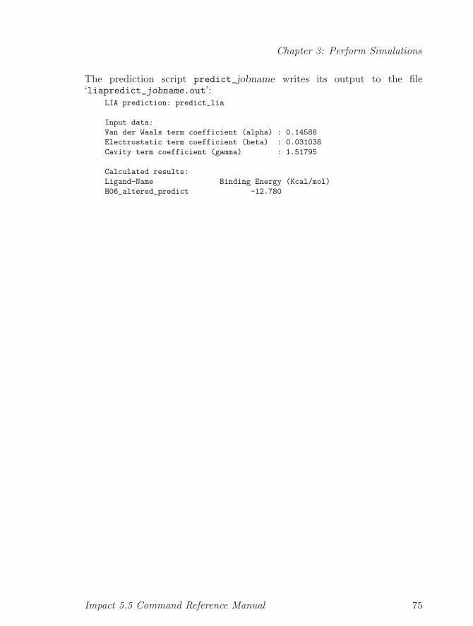
Chapter 3: Perform Simulations
The prediction script predict_jobname writes its output to the file‘liapredict_jobname.out’:
LIA prediction: predict_lia
Input data:
Van der Waals term coefficient (alpha) : 0.14588
Electrostatic term coefficient (beta) : 0.031038
Cavity term coefficient (gamma) : 1.51795
Calculated results:
Ligand-Name Binding Energy (Kcal/mol)
H06_altered_predict -12.780
Impact 5.5 Command Reference Manual 75
Chapter 3: Perform Simulations
3.5 Task Docking (DOCK or GLIDE)The DOCK task, also called Glide (for Grid-based LIgand Docking withEnergetics), is the heart of Schrodinger’s Glide product. The docking al-gorithm searches for favorable interactions between a (typically) small lig-and molecule and a (typically) larger receptor molecule, usually a protein.The ligand and receptor typically occupy separate Impact species, thoughthey may also be separate molecules in the same species. The ligand mustbe a single Impact molecule, while the receptor may include more than onemolecule, e.g. a protein and a cofactor. Because of the relative complexity ofthis task, several examples of its use are included in this section, in additionto the usual meta-examples under each subtask or command.
3.5.1 Description of the Docking Algorithm
The docking procedure for a given ligand molecule runs through two stages,which we refer to as rough scoring and grid energy optimization. Each stagerelies on grids representing the receptor binding site, but the grids for onestage are not the same as for the other. As in other docking programssuch as DOCK (E.C. Meng, B.K. Shoichet and I.D. Kuntz, J. Comput.Chem. 13, 505, 1992) and Autodock (G.M. Morris, D.S. Goodsell, R.S.Halliday, R. Huey, W.E. Hart, R.K. Belew and A.J. Olson, J. Comput.Chem. 19, 1639, 1998), the grids can be precomputed and stored on disk, soit is unnecessary to read in the receptor molecule, and perform computationson it, repeatedly for multiple ligands or multiple conformers of the sameligand. Using grids also makes computing the ligand-receptor interactionenergy an O(nlig) rather than O(nlig ∗ nprot) process, where nlig is thenumber of atoms in the ligand and nprot is the number of atoms in thereceptor.In a typical project, the user will set up the grids in one Glide run, anddock ligands in one or more subsequent runs, as described below. It is notcurrently possible to set up grids and dock ligands in the same run. (See“Important Operational Notes” in the Glide Technical Notes.) In all cases,the user should specify saving the grids to disk whenever calculating them.In the current version of Glide, there are two possible ways to incorporateligand flexibility: include multiple conformers of a given ligand in the inputto Impact, or use the program’s internal conformation generator startingwith a single conformer of a given ligand. We strongly recommend thelatter. It covers conformational space systematically, and by clustering con-formers that have a common “core,” it runs much faster than docking thesame number of externally generated conformers. In conjunction with in-ternal conformation generation, Glide also allows ligand torsional flexibilityduring the optimization of the ligand-receptor interaction energy, and werecommend using this feature. Future versions of Glide will allow for recep-tor flexibility; for now, scaling of the van der Waals radii of receptor atoms(also available for ligand atoms) mimics some possible motions of the re-
76 Impact 5.5 Command Reference Manual
Chapter 3: Perform Simulations
ceptor, such as “breathing” to fit a larger ligand than the one present in aparticular co-crystallized structure.In addition to generating or processing multiple conformations of a givenmolecule, Glide can also dock, and compare the predicted binding affinitiesof, multiple ligand molecules in a single Impact run, using a loop in the inputscripting language (DICE). In the case of externally generated conformers,the same loop can run over a list of input structures that includes bothdifferent molecules and different conformers of each, using Impact’s buildprimary check syntax to determine which is which. (The input structuresfor internal conformation generation can in principle also include multipleconformers of the same ligand, but there is no reason to do so, and we donot recommend it.)The first stage of the algorithm, known as screening or rough scoring, mea-sures the geometric “fit” between the ligand and receptor molecules, and ap-proximations to specific interactions between them such as hydrogen bonds.The grids for the rough-scoring stage contain values of a rough score functionrepresenting how favorable or unfavorable it would be to place ligand atomsof given general types (e.g. polar hydrogens, hydrogen bond acceptors, hy-drophobic heavy atoms) in given elementary cubes of the grid. These gridshave a constant spacing, which defaults to 1 A. The rough score for a givenpose (position and orientation) of the ligand relative to the receptor is sim-ply the sum of the appropriate grid scores for each of its atoms. By analogywith energy, favorable scores are negative, and the lower (more negative) thebetter.The screening stage is actually a hierarchical series of filters that drasticallynarrow down the set of poses that are considered candidates for docking.A given pose is defined by three Cartesian coordinates of the ligand center,and three Euler angles. The ligand center is taken to be the midpoint of thediameter, which in turn is taken to be the longest line segment connectingtwo ligand atoms. Although some of the commands in the docking task usethe abbreviation cm in keywords to refer to this point, this definition is verydifferent from the centroid or “center of mass” of the ligand atom positions.Note also that it may be far from the actual position of any ligand atom. (Infact, if the ligand “wraps around” a convex portion of the receptor surface,the ligand center may be inside the receptor.) The Cartesian coordinatesof the center position are defined relative to the origin of coordinates in thereceptor coordinate file. The Euler angles ψ and θ are defined relative to anorientation in which the ligand diameter points along the z-axis; the φ angle(rotation of the ligand about its diameter) is taken to be zero in the inputcoordinates of the ligand. This biases one of the six coordinates in favor ofits input value, but we have not found this to be a problem even when theinput is the “correct answer”, e.g., a co-crystallized ligand-receptor complex.It is also possible to choose the grid points to include the ligand centercoordinates in the input, which introduces additional bias. The ligand poses
Impact 5.5 Command Reference Manual 77
Chapter 3: Perform Simulations
that constitute the search space for the screening step correspond to discretevalues of these six coordinates. The ligand center is placed at selected pointson the rough-score grid, with the default being every other point. The ψ andθ angles are taken from the polar coordinates of a set of points uniformlydistributed on the unit sphere (by default, a set of 302 such points from thefile ‘grid.pts’), and φ is distributed evenly between 0 and 360 degrees, withthe default being 25 values at intervals of 14.4 degrees.
Early filters in the screening stage are purely geometric, weeding out sitesfor the ligand center that have no chance of being good docking positions,because they are too far from the receptor or have no chance of shape com-plementarity. The later filters involve evaluating the rough-score function onsubsets of the ligand atoms, such as those near the diameter (whose scoresshould be independent of φ, so ruling them out for one value of φ kills 25poses based on as few as 2 ligand atoms), or hydrogen-bonding atoms (orothers expected to make major contributions to favorable scores, so that ifthe score is not favorable for the subset, there’s no point in evaluating it forthe rest of the ligand). Effective application of the filters can rapidly reducethe number of poses to be considered from hundreds of thousands or millionsto a few dozen (or less), before evaluating the full rough-score function onall the ligand atoms in any pose.
By default, and by our recommendation, the rough-scoring function is de-fined on a 1 A grid. In the interest of execution speed, the default sitesfor the ligand center occupy a 2 A grid consisting of alternating points ofthe rough-score grid. The default rough-score function is based on count-ing receptor atoms of various types within certain distances of grid points,and thus has a step-function character, and can vary considerably from onegrid point to the next. Therefore a pose that gets an unfavorable score maybe very close in space to one that would get a favorable score, and possiblywould minimize to a good docked configuration. If the favorable score occursfor a pose with the ligand center on a skipped grid point, it might never befound. This is particularly likely for receptors with tight binding pockets.
To address this potential problem, Glide allows two enhancements of therough-score function, which we call greedy scoring and pose refinement.Both involve examining scores at grid points surrounding the current po-sitions of ligand atoms, but avoid the considerable expense of moving everyatom of every pose through a 3x3x3 set of neighboring points.
Greedy scoring involves setting up alternative rough-score grids, which ateach grid point incorporate some “influence” of the most favorable score inthe 3x3x3 neighborhood of the central grid point. To construct a “greedygrid” given the original rough-score grid, the algorithm first finds the mostfavorable (lowest or most negative) score in the 3x3x3 neighborhood. Thevalue stored in the greedy grid at the given grid point is then a linear com-bination of the original grid value and the best neighboring one: greedy = x
78 Impact 5.5 Command Reference Manual
Chapter 3: Perform Simulations
* best + (1−x) * original. The default is x = 0.33, but the user may specifyany value between 0 (the same as non-greedy scoring) and 1, inclusive.Pose refinement is a method for evaluating the rough-scores of selected poseson a finer translational grid than the default. The refinement step takeseach pose that passed all the screening tests, and moves the ligand centerto neighboring grid points. The default step size for these moves is one gridpoint (1 A), which with the default spacing of ligand center sites means thatall the poses it covers other than the central one were skipped in the originalsearch. If any of these “refined” poses gets a better score than the original(central) one, the algorithm passes the best such pose on to subsequent steps,instead of the central one.Greedy scoring adds computational overhead for reading (and the first time,computing and writing) the greedy grid, and also, in our tests, about 10–20%to the CPU time for screening poses of a given conformation (presumablybecause more poses pass some of the filters). Pose refinement adds a negli-gible amount of time to a multiple-conformation or multiple-ligand run, andtends to decrease the number of poses that need to be passed to minimiza-tion. Because they significantly enhance the likelihood of finding good poses,we recommend using both features.In a run with multiple externally-generated conformations of a given ligand,the program executes most efficiently (in both time and memory use) if itperforms the (greedy) rough-score calculation for all the conformers first,keeps some specified total number of best poses over all the conformers, andthen proceeds to pose refinement (and subsequent steps) only on those bestoverall poses of the given ligand. For internal conformation generation, therough-scoring algorithm treats all the conformers for a given input ligandin tandem, so it automatically does pose refinement only on the best posesover all conformers.The second stage of the docking algorithm begins with evaluation and min-imization of a grid approximation to the nonbonded interaction energy be-tween the ligand and the receptor. The grids store the values of the electro-static potential due to the receptor atoms (with a constant or linear dielec-tric, at user option), and the attractive and repulsive parts of the Lennard-Jones energy. The docking algorithm is implemented only for the OPLS-AAforce field. Attempting to use it with a different force field will result in anerror exit from Impact.The energy values are defined on an adaptive grid, with a finer spacing closeto the receptor for accuracy where the potential energy is changing rapidly,and coarser far from the receptor to save time and space where the potentialvaries slowly (and contributes less to the total in any case). The default forthe finest grid spacing is 0.4 A, increasing to 3.2 A in three steps. At useroption, the grid energy also incorporates smoothing functions that eliminatethe singularity in the potential energy at zero distance, and thus softenthe hard walls that could otherwise trap the algorithm in local minima. We
Impact 5.5 Command Reference Manual 79
Chapter 3: Perform Simulations
recommend starting the grid-energy minimization on the smoothed potentialsurface, and annealing to the full OPLS-AA grid energy. To accomplish this,include the subtask smooth anneal 2 in the DOCK task.The energy evaluations and minimizations use a continuous function for theenergy, obtained by linear interpolation among the values at the corners ofthe cube of grid points surrounding each ligand atom position. The positionand orientation coordinates of the ligand are varied continuously during theminimization. With Glide’s internal conformation generation feature, wealso provide, and recommend, the option of varying ligand dihedral anglesduring the minimization.Glide performs its calculations in the context of two concentric rectangularboxes, representing different aspects of the receptor active site. The bound-ing box (or “ligand center box”) delimits the space in which the ligand center(as defined above) can move. The size of this box determines the size of thespace that the algorithm explores, and thus the amount of computer time(and to some extent memory) it takes to execute, so to optimize perfor-mance, it should be as small as the user’s knowledge of the binding site willallow. Around this bounding box, the enclosing box is the space in whichGlide defines and calculates the grid values for the rough-score and energyfunctions. The algorithm rejects a candidate site for the ligand center ifany conformation and pose of the ligand, with its center at that site, wouldhave any atom outside the enclosing box. Therefore it is important to makethe enclosing box large enough relative to the bounding box so that the lig-and will fit inside it at all likely sites for its center. Memory restrictions,unfortunately, limit the size of the enclosing box to 50 A on a side.The location and dimensions of the bounding and enclosing boxes are eithercalculated from the coordinates of the receptor atoms in residues that theuser specifies as active, taken directly from user specifications via the boxkeyword in the receptor and/or screen subtasks, or read from grid filespreviously stored to disk.
3.5.2 Example 1: Set up grids
The following example sets up grids based on the receptor in the co-crystallized thrombin-inhibitor complex contained in PDB entry 1ETS. Sub-sequent examples dock ligands to this receptor, as represented by these grids.In the text accompanying these examples, we briefly explain the subtasks ofthe DOCK task. In later sections devoted to each subtask, we provide moredetailed descriptions, and information about overriding defaults for param-eters or options not shown here. It is important to note that all of thesubtasks except confgen, simil, and run simply set up the specificationsand parameters for the docking run; except for confgen, which immediatelygenerates conformations, and simil, which immediately generates or readssimilarity weights, Impact does not perform any docking calculations untilit encounters run. Thus every invocation of the DOCK task must end with
80 Impact 5.5 Command Reference Manual
Chapter 3: Perform Simulations
the run subtask. Note also that every subtask of this task occupies a singlelogical line of the Impact input file. Thus it is crucial to include the hyphensto indicate continuation of the command (subtask) on the next physicalline. Furthermore, it is important to remember that each physical line ofthe Impact input file is truncated after 132 characters. For this reason, allfile names in the examples shown here are on separate physical lines (withhyphens for continuation as needed). Users must insure that all their filepathnames (including directories) are short enough to fit in this limit, whichtypically means 128 or 130 characters in order to leave room for quotationmarks and/or hyphens. The Maestro user interface will refuse to write anImpact input file, or start the corresponding job, if the user specifies a path-name that is too long. We recommend that users who have complicateddirectory structures should either run Impact in directories close to wheretheir files are located, or if this is not practical, use such Unix system fea-tures as symbolic links or environment variables to shorten the names to bewritten to the Impact input file.It will be noted that unlike most Impact input files, none of the examplesin this section contains a setmodel task. This is because Glide computesenergies differently from other tasks such as minimize and dynamics. Itdoes so by precomputing receptor grids using the OPLS-AA force field, andreading (and interpolating) energies from them for ligand atoms, rather thanlooping over atom pairs. For this reason, this task does not require setmodelto specify features and parameters of the energy function.
Impact 5.5 Command Reference Manual 81
Chapter 3: Perform Simulations
write file "1ets_single_grid.out" -
title "1ets_single_grid" *
CREATE
build primary name recep type auto -
read maestro file -
"1ets_single_grid.mae" -
tag REC_
build types name recep
QUIT
DOCK
smooth anneal 2
receptor name recep -
writef -
"1ets_single_grid" -
protvdwscale factor 0.900000 ccut 0.250000 -
box center read xcent -37.510494 ycent -28.946030 zcent 44.411289 -
boxxrange 27.346889 boxyrange 27.346889 boxzrange 27.346889 -
actxrange 27.346889 actyrange 27.346889 actzrange 27.346889
screen greedy -
box center read xcent -37.510494 ycent -28.946030 zcent 44.411289 -
ligxrange 12.000000 ligyrange 12.000000 ligzrange 12.000000 -
writescreen -
"1ets_single_grid.save" -
writegreed -
"1ets_single_grid_greedy.save"
parameter clean
final glidescore
run
QUIT
END
smooth Indicates that the calculation of the energy grids should incor-porate short-distance smoothing functions. anneal 2 indicatesthat the grids should include two different potential-energy sur-faces, one with smoothing and one without. In a DOCK task to dogrid-energy optimization, smooth anneal 2 means that the op-timization should start on the smoothed surface and end on theunsmoothed one. Alternatively, a subsequent DOCK task couldinclude smooth anneal 1 to use only the smoothed surface, oromit the smooth subtask in order to use only the unsmoothedsurface; but we strongly recommend using smooth anneal 2 inall cases.
receptor Specifies the receptor molecule(s) and its active site.name recep
Indicates that the receptor is in the Impact speciesdesignated recep in the preceding CREATE task. If
82 Impact 5.5 Command Reference Manual
Chapter 3: Perform Simulations
this species contained more than one molecule, thenby default the receptor would include all moleculesin the species; specifying mole mol in this subtaskwould restrict the receptor to that single molecule.
writef 1ets_single_gridIndicates that the energy grids will be writ-ten to files whose names are built fromthe base 1ets_single_grid. Specifically,‘1ets_single_grid.grd’ will contain struc-tural information about the adaptive griditself (size and coordinates of each gridbox), ‘1ets_single_grid_vdw.fld’ willcontain the Lennard-Jones energy grid,‘1ets_single_grid_coul.fld’ will contain theCoulomb potential with a dielectric constant of 1,and ‘1ets_single_grid_coul2.fld’ will containthe Coulomb potential with a distance-dependentdielectric of 1 ∗ r. In addition, Impact willwrite the receptor structure to a Maestro formatfile, ‘1ets_single_grid_recep.mae’, for use insubsequent Glide jobs. (To compute and write justone of the Coulomb files and not the other, usethe keyword writecdie for the constant dielectricor writerdie for the r-dependent dielectric.writerdie overrides writecdie, so if you specifyboth, only the r-dielectric will be computed andwritten. To specify a dielectric other than 1 or 1∗r,use the dielco keyword in the minimize subtask.)NOTE: The files read and written by Glide can bevery large (tens of megabytes). To save space onuser disks, and also to save time (network latency)in environments where the user disk is on a serverother than the local CPU, we recommend readingand writing these files on local “scratch” diskswhile running Impact, and transferring them tomore “permanent” locations separately.
protvdwscaleSpecifies a scale factor (factor) for the van derWaals radii of nonpolar receptor atoms. All atomswhose partial charge (absolute value) is less thanccut are considered nonpolar for this purpose.Specifying factor < 1.0, by effectively makingreceptor atoms seem smaller to ligands, is a wayof letting the receptor “breathe” to accommodate
Impact 5.5 Command Reference Manual 83
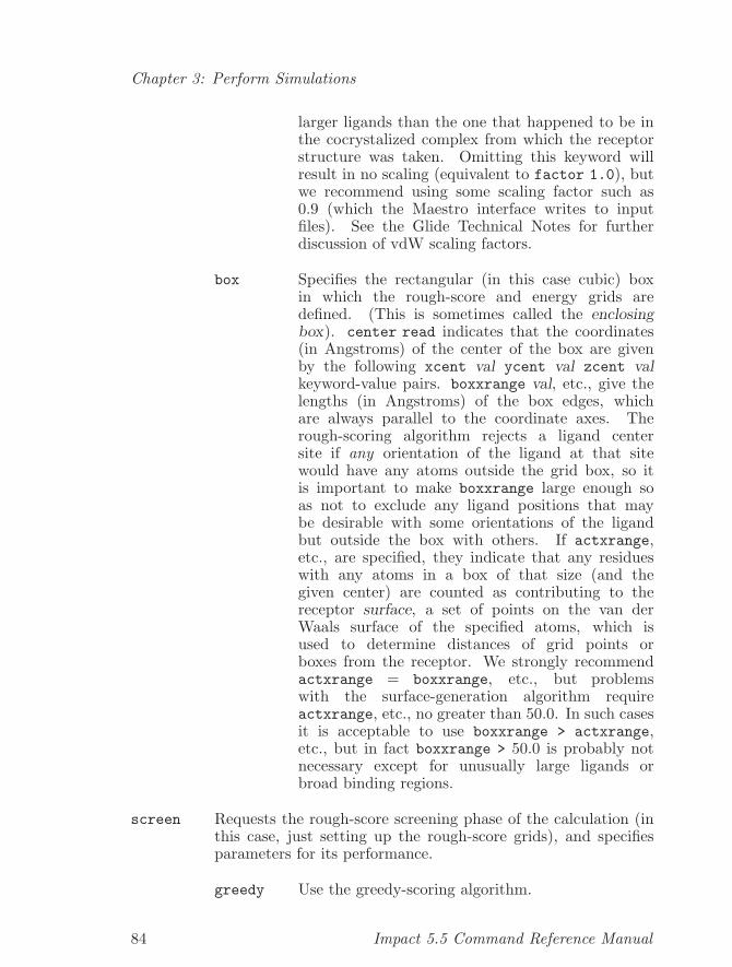
Chapter 3: Perform Simulations
larger ligands than the one that happened to be inthe cocrystalized complex from which the receptorstructure was taken. Omitting this keyword willresult in no scaling (equivalent to factor 1.0), butwe recommend using some scaling factor such as0.9 (which the Maestro interface writes to inputfiles). See the Glide Technical Notes for furtherdiscussion of vdW scaling factors.
box Specifies the rectangular (in this case cubic) boxin which the rough-score and energy grids aredefined. (This is sometimes called the enclosingbox). center read indicates that the coordinates(in Angstroms) of the center of the box are givenby the following xcent val ycent val zcent valkeyword-value pairs. boxxrange val, etc., give thelengths (in Angstroms) of the box edges, whichare always parallel to the coordinate axes. Therough-scoring algorithm rejects a ligand centersite if any orientation of the ligand at that sitewould have any atoms outside the grid box, so itis important to make boxxrange large enough soas not to exclude any ligand positions that maybe desirable with some orientations of the ligandbut outside the box with others. If actxrange,etc., are specified, they indicate that any residueswith any atoms in a box of that size (and thegiven center) are counted as contributing to thereceptor surface, a set of points on the van derWaals surface of the specified atoms, which isused to determine distances of grid points orboxes from the receptor. We strongly recommendactxrange = boxxrange, etc., but problemswith the surface-generation algorithm requireactxrange, etc., no greater than 50.0. In such casesit is acceptable to use boxxrange > actxrange,etc., but in fact boxxrange > 50.0 is probably notnecessary except for unusually large ligands orbroad binding regions.
screen Requests the rough-score screening phase of the calculation (inthis case, just setting up the rough-score grids), and specifiesparameters for its performance.
greedy Use the greedy-scoring algorithm.
84 Impact 5.5 Command Reference Manual
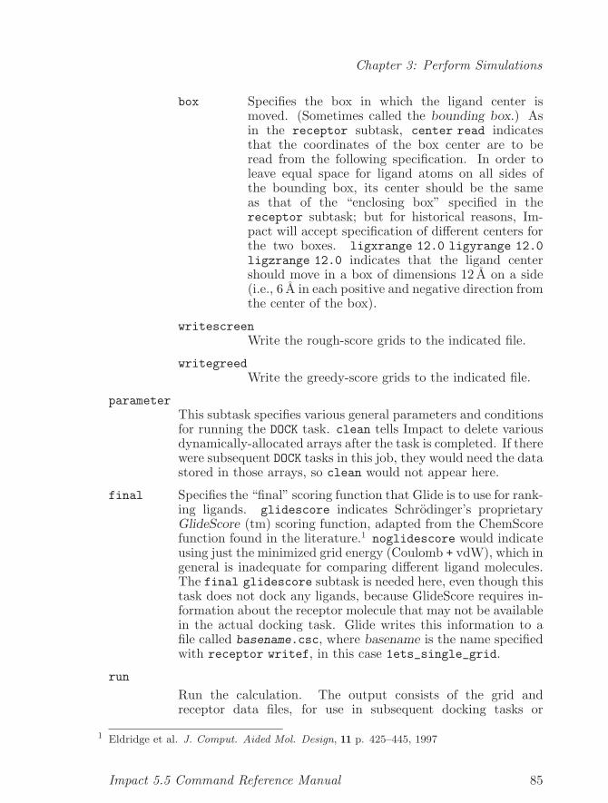
Chapter 3: Perform Simulations
box Specifies the box in which the ligand center ismoved. (Sometimes called the bounding box.) Asin the receptor subtask, center read indicatesthat the coordinates of the box center are to beread from the following specification. In order toleave equal space for ligand atoms on all sides ofthe bounding box, its center should be the sameas that of the “enclosing box” specified in thereceptor subtask; but for historical reasons, Im-pact will accept specification of different centers forthe two boxes. ligxrange 12.0 ligyrange 12.0ligzrange 12.0 indicates that the ligand centershould move in a box of dimensions 12 A on a side(i.e., 6 A in each positive and negative direction fromthe center of the box).
writescreenWrite the rough-score grids to the indicated file.
writegreedWrite the greedy-score grids to the indicated file.
parameterThis subtask specifies various general parameters and conditionsfor running the DOCK task. clean tells Impact to delete variousdynamically-allocated arrays after the task is completed. If therewere subsequent DOCK tasks in this job, they would need the datastored in those arrays, so clean would not appear here.
final Specifies the “final” scoring function that Glide is to use for rank-ing ligands. glidescore indicates Schrodinger’s proprietaryGlideScore (tm) scoring function, adapted from the ChemScorefunction found in the literature.1 noglidescore would indicateusing just the minimized grid energy (Coulomb + vdW), which ingeneral is inadequate for comparing different ligand molecules.The final glidescore subtask is needed here, even though thistask does not dock any ligands, because GlideScore requires in-formation about the receptor molecule that may not be availablein the actual docking task. Glide writes this information to afile called basename.csc, where basename is the name specifiedwith receptor writef, in this case 1ets_single_grid.
run
Run the calculation. The output consists of the grid andreceptor data files, for use in subsequent docking tasks or
1 Eldridge et al. J. Comput. Aided Mol. Design, 11 p. 425–445, 1997
Impact 5.5 Command Reference Manual 85
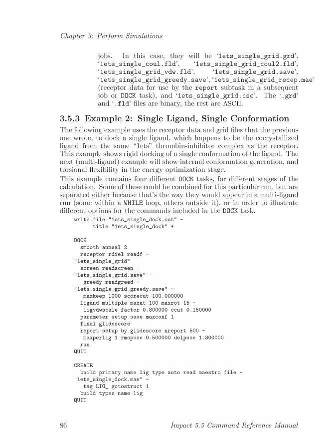
Chapter 3: Perform Simulations
jobs. In this case, they will be ‘1ets_single_grid.grd’,‘1ets_single_coul.fld’, ‘1ets_single_grid_coul2.fld’,‘1ets_single_grid_vdw.fld’, ‘1ets_single_grid.save’,‘1ets_single_grid_greedy.save’, ‘1ets_single_grid_recep.mae’(receptor data for use by the report subtask in a subsequentjob or DOCK task), and ‘1ets_single_grid.csc’. The ‘.grd’and ‘.fld’ files are binary, the rest are ASCII.
3.5.3 Example 2: Single Ligand, Single Conformation
The following example uses the receptor data and grid files that the previousone wrote, to dock a single ligand, which happens to be the cocrystallizedligand from the same “1ets” thrombin-inhibitor complex as the receptor.This example shows rigid docking of a single conformation of the ligand. Thenext (multi-ligand) example will show internal conformation generation, andtorsional flexibility in the energy optimization stage.This example contains four different DOCK tasks, for different stages of thecalculation. Some of these could be combined for this particular run, but areseparated either because that’s the way they would appear in a multi-ligandrun (some within a WHILE loop, others outside it), or in order to illustratedifferent options for the commands included in the DOCK task.
write file "1ets_single_dock.out" -
title "1ets_single_dock" *
DOCK
smooth anneal 2
receptor rdiel readf -
"1ets_single_grid"
screen readscreen -
"1ets_single_grid.save" -
greedy readgreed -
"1ets_single_grid_greedy.save" -
maxkeep 1000 scorecut 100.000000
ligand multiple maxat 100 maxrot 15 -
ligvdwscale factor 0.800000 ccut 0.150000
parameter setup save maxconf 1
final glidescore
report setup by glidescore nreport 500 -
maxperlig 1 rmspose 0.500000 delpose 1.300000
run
QUIT
CREATE
build primary name lig type auto read maestro file -
"1ets_single_dock.mae" -
tag LIG_ gotostruct 1
build types name lig
QUIT
86 Impact 5.5 Command Reference Manual
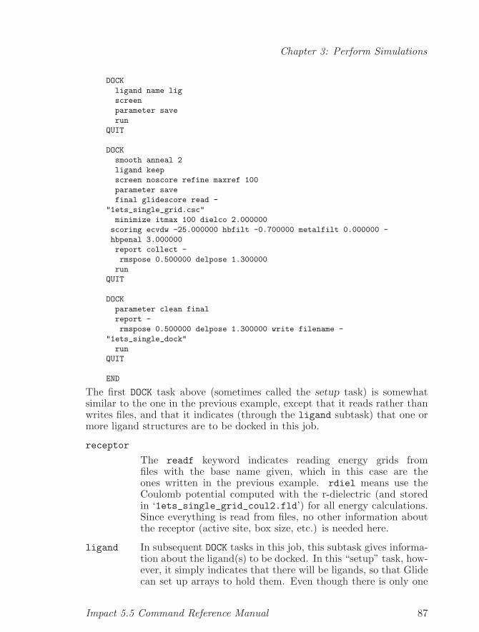
Chapter 3: Perform Simulations
DOCK
ligand name lig
screen
parameter save
run
QUIT
DOCK
smooth anneal 2
ligand keep
screen noscore refine maxref 100
parameter save
final glidescore read -
"1ets_single_grid.csc"
minimize itmax 100 dielco 2.000000
scoring ecvdw -25.000000 hbfilt -0.700000 metalfilt 0.000000 -
hbpenal 3.000000
report collect -
rmspose 0.500000 delpose 1.300000
run
QUIT
DOCK
parameter clean final
report -
rmspose 0.500000 delpose 1.300000 write filename -
"1ets_single_dock"
run
QUIT
END
The first DOCK task above (sometimes called the setup task) is somewhatsimilar to the one in the previous example, except that it reads rather thanwrites files, and that it indicates (through the ligand subtask) that one ormore ligand structures are to be docked in this job.
receptor
The readf keyword indicates reading energy grids fromfiles with the base name given, which in this case are theones written in the previous example. rdiel means use theCoulomb potential computed with the r-dielectric (and storedin ‘1ets_single_grid_coul2.fld’) for all energy calculations.Since everything is read from files, no other information aboutthe receptor (active site, box size, etc.) is needed here.
ligand In subsequent DOCK tasks in this job, this subtask gives informa-tion about the ligand(s) to be docked. In this “setup” task, how-ever, it simply indicates that there will be ligands, so that Glidecan set up arrays to hold them. Even though there is only one
Impact 5.5 Command Reference Manual 87
Chapter 3: Perform Simulations
ligand in this case, the multiple keyword must precede maxatand maxrot, which give the maximum number of atoms and ro-tatable bonds allowed in any ligand molecule in the current job.If we were indeed looping over multiple ligands, any one thatexceeded these limits would be skipped. In addition, maxat isused in allocating storage for the ligand atom coordinates. Theligvdwscale keyword invokes scaling of the ligand vdW radiiused in energy calculations, similar to protvdwscale above. Asfor the protein, omitting this keyword results in setting factor1.0 (no scaling), but we recommend using a scale factor < 1.0,and the Maestro interface writes factor 0.8, as shown. Again,see the Glide Technical Notes for further discussion.
parameterThe setup keyword indicates that no actual calculations are tobe done in this invocation of the task. Instead, the receptor andligand data are simply read in and stored in dynamically allo-cated arrays. (The sizes of most of these arrays are read fromthe same grid files that contain their contents.) The save key-word indicates that these arrays should be retained in memoryfor use by subsequent invocations of the task. The maxconf key-word gives the dimension of dynamically allocated arrays that,in general, store information for multiple ligands or (externallygenerated) conformations. In this case, maxconf 1 indicates asingle ligand structure.
screen As with readf above, readscreen and readgreed here meanread the rough-score grids from the indicated files, and we don’tneed a box specification because it’s in the same files. Thefollowing additional parameters give details of the rough-scorescreening task to follow.
maxkeep Indicates the maximum number of ligand poses tobe passed to the energy minimization. The numberactually kept may be less than this, because fewerposes pass the various rough-score filters.
scorecut Rough-score window for passing poses togrid-energy optimization. A pose survives if itsrough-score is within scorecut of the best poseaccumulated so far.
report Gives instructions for the “reporting” (output) of docked ligandposes (A pose is the structure of a single conformation of asingle ligand, in a single position and orientation relative to thereceptor). The setup task requires some information about whatis to be reported and how.
88 Impact 5.5 Command Reference Manual
Chapter 3: Perform Simulations
setup Indicates that we’re specifying the reporting func-tion here. Of course we can’t actually collect datafor the report (much less write it to output files) un-til we’ve actually docked the ligands. But we needto allocate space for the report data, etc.
by glidescoreIndicates that the poses to be reported will be sortedin order of the GlideScore scoring function.
nreport The maximum number of poses to report. (Theactual number may be smaller because fewer passall screening or scoring tests, or because of themaxperlig keyword.
maxperligThe maximum number of poses to report for anygiven ligand molecule. maxperlig 1 is particularlyuseful for rapid screening of large databases, produc-ing one pose for each of the nreport best-scoring lig-ands, which can then be subjected to more detailedcalculations.
rmsposedelpose The rough-score and energy-optimization stages of
a Glide may generate poses for a given ligand thatare similar to each other. In order to avoid dupli-cation in the report, these keyword-value pairs in-dicate that two poses of the same ligand are to beconsidered distinct (and thus both reported if theyotherwise qualify) only if the RMS deviation of theiratomic positions exceeds the rmspose value, or themaximum deviation for any atom exceeds delpose.These keyword-value pairs must appear in every oc-curence of the report subtask in a given Glide inputfile.
The second DOCK task above runs the rough-score screening (except for poserefinement). Glide knows that it should do this (rather than just allocatearrays) because there is no setup keyword in the parameter subtask.
ligand name ligCopy the indicated Impact species into the Glide ligand arrays.
screen Run the rough-score screening using the parameters and infor-mation specified in the previous DOCK task.
The third DOCK task runs pose refinement and grid-energy optimization.
Impact 5.5 Command Reference Manual 89
Chapter 3: Perform Simulations
smooth anneal 2Needed here to tell Glide to use both the smoothed and “hard”potential energy surfaces in the actual minimization. It’s possi-ble to use smooth anneal 2 in the first task in order to calculateor read both surfaces, but smooth anneal 1 here to use only thesmoothed one, or leave out the smooth subtask here to use onlythe hard surface.
ligand keepContinue to run calculations on the ligand structure used in theprevious DOCK task, rather than reading in a new one.
screen
noscore Don’t do the whole rough-score process here, be-cause we did it in a previous task.
refine Use pose refinement.
maxref Maximum number of poses to keep after pose refine-ment.
minimize Minimize the Coulomb+vdW interaction energy (interpolated onthe grids) for each ligand pose that survives through the rough-score and refinement steps.
itmax Maximum number of conjugate-gradient iterations
dielco Dielectric coefficient. If cdiel appears in thereceptor subtask above, this is the dielectricconstant. If rdiel, the dielectric is this num-ber multiplied by the interatomic distance inAngstroms.
scoring Various filters for keeping poses after energy minimization.
ecvdw Reject any pose whose minimized Coul+vdW energyis greater (in this case, less negative) than this num-ber.
hbfilt Reject any pose for which the hydrogen-bond con-tribution to GlideScore is greater than this number.
metalfiltReject any pose for which the metal-binding contri-bution to GlideScore is greater than this number
hbpenal Assign this penalty in GlideScore for each buriedpolar interaction.
report collectAfter minimization, and in this case GlideScore evaluation, col-lect data on top poses for final output. For a single ligand, this
90 Impact 5.5 Command Reference Manual
Chapter 3: Perform Simulations
could be combined with the report write subtask in the nexttask. But for a loop over multiple ligands, collection is doneinside the loop for each ligand, and final output is done once atthe end of the job, outside the loop.
The fourth DOCK task writes the final output.
parameter clean finalDelete dynamically allocated arrays at the end of the task. Thefinal keyword insures that the Glide report function is executedeven if the last ligand’s structure was problematic.
report ... write filename ...Write the best poses (up to nreport of them, but subject tomaxperlig and survival through all scoring filters) to the outputfiles. For filename base, write the receptor structure and theligand pose structures to base pv.mae, and a summary of theposes and their scores to base.rept. The user can view the poseson screen, in conjunction with the receptor, by using the GlidePose Viewer, available from the Maestro “Analysis” menu.
3.5.4 Example 3: Multiple Ligands, Flexible Docking
The above example treats a single conformation of a single ligand, to find themost favorable pose for docking to the given receptor. Probably the morecommon use of Glide is to determine which of a number of conformations,or which ligand of a number of candidates, has the most favorable interac-tion with the receptor. The DOCK task can be invoked repeatedly to handlemultiple input ligand structures, as in the loop shown below using the DICEscripting language. (See Chapter 4 [Advanced Input Scripts], page 131 fordetails of DICE.) We recommend using a loop as shown here, over multipleligands in a single file (Maestro or MDL SD format), with each structure adifferent ligand, and using Impact’s internal conformation generator (sub-task confgen) and torsional flexibility during grid-energy optimization (flexkeyword in minimize subtask) to sample the conformational space of eachligand in turn.After the example, we describe the ways in which this example differs fromthe single-structure example above.
write file "1ets_example_mult.out" -
title "1ets_example_mult" *
PUT 0 INTO ’buildcheck’
PUT 1 INTO ’startlig’
PUT 0 INTO ’endlig’
PUT -1 INTO ’strucseq’
DOCK
Impact 5.5 Command Reference Manual 91
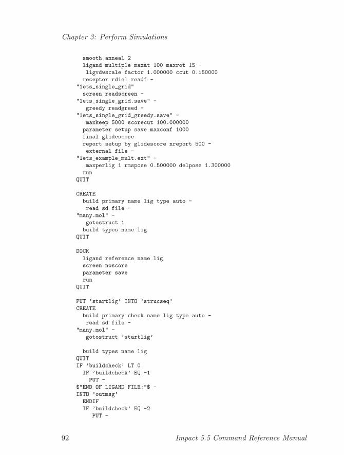
Chapter 3: Perform Simulations
smooth anneal 2
ligand multiple maxat 100 maxrot 15 -
ligvdwscale factor 1.000000 ccut 0.150000
receptor rdiel readf -
"1ets_single_grid"
screen readscreen -
"1ets_single_grid.save" -
greedy readgreed -
"1ets_single_grid_greedy.save" -
maxkeep 5000 scorecut 100.000000
parameter setup save maxconf 1000
final glidescore
report setup by glidescore nreport 500 -
external file -
"1ets_example_mult.ext" -
maxperlig 1 rmspose 0.500000 delpose 1.300000
run
QUIT
CREATE
build primary name lig type auto -
read sd file -
"many.mol" -
gotostruct 1
build types name lig
QUIT
DOCK
ligand reference name lig
screen noscore
parameter save
run
QUIT
PUT ’startlig’ INTO ’strucseq’
CREATE
build primary check name lig type auto -
read sd file -
"many.mol" -
gotostruct ’startlig’
build types name lig
QUIT
IF ’buildcheck’ LT 0
IF ’buildcheck’ EQ -1
PUT -
$"END OF LIGAND FILE:"$ -
INTO ’outmsg’
ENDIF
IF ’buildcheck’ EQ -2
PUT -
92 Impact 5.5 Command Reference Manual
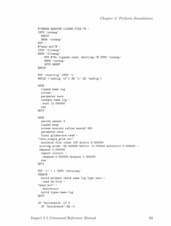
Chapter 3: Perform Simulations
$"ERROR READING LIGAND FILE:"$ -
INTO ’outmsg’
ENDIF
SHOW ’outmsg’
PUT -
$"many.mol"$ -
INTO ’filemsg’
SHOW ’filemsg’
PUT $"No ligands read; aborting."$ INTO ’outmsg’
SHOW ’outmsg’
GOTO ABORT
ENDIF
PUT ’startlig’ INTO ’i’
WHILE (’endlig’ LT 1 OR ’i’ LE ’endlig’)
DOCK
ligand name lig
screen
parameter save
confgen name lig -
ecut 12.000000
run
QUIT
DOCK
smooth anneal 2
ligand keep
screen noscore refine maxref 400
parameter save
final glidescore read -
"1ets_single_grid.csc"
minimize flex itmax 100 dielco 2.000000
scoring ecvdw -25.000000 hbfilt -0.700000 metalfilt 0.000000 -
hbpenal 3.000000
report collect -
rmspose 0.500000 delpose 1.300000
run
QUIT
PUT ’i’ + 1 INTO ’strucseq’
CREATE
build primary check name lig type auto -
read sd file -
"many.mol" -
nextstruct
build types name lig
QUIT
IF ’buildcheck’ LT 0
IF ’buildcheck’ EQ -1
Impact 5.5 Command Reference Manual 93
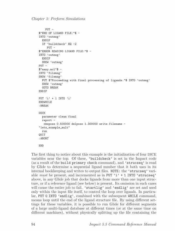
Chapter 3: Perform Simulations
PUT -
$"END OF LIGAND FILE:"$ -
INTO ’outmsg’
ENDIF
IF ’buildcheck’ EQ -2
PUT -
$"ERROR READING LIGAND FILE:"$ -
INTO ’outmsg’
ENDIF
SHOW ’outmsg’
PUT -
$"many.mol"$ -
INTO ’filemsg’
SHOW ’filemsg’
PUT $"Proceeding with final processing of ligands."$ INTO ’outmsg’
SHOW ’outmsg’
GOTO BREAK
ENDIF
PUT ’i’ + 1 INTO ’i’
ENDWHILE
:BREAK
DOCK
parameter clean final
report -
rmspose 0.500000 delpose 1.300000 write filename -
"1ets_example_mult"
run
QUIT
:ABORT
END
The first thing to notice about this example is the initialization of four DICEvariables near the top. Of these, ’buildcheck’ is set in the Impact code(as a result of the build primary check command), and ’strucseq’ is readby Glide to determine a sequential ligand number that it both uses in itsinternal bookkeeping and writes to output files. NOTE: the ’strucseq’ vari-able must be present, and incremented as in PUT ’i’ + 1 INTO ’strucseq’above, in any Glide job that docks ligands from more than one input struc-ture, or if a reference ligand (see below) is present. Its omission in such caseswill cause the entire job to fail. ’startlig’ and ’endlig’ are set and usedonly within the input file itself, to control the loop over ligands. In particu-lar, PUT 0 INTO ’endlig’, combined with the subsequent WHILE command,means loop until the end of the ligand structure file. By using different set-tings for these variables, it is possible to run Glide for different segmentsof a large multi-ligand database at different times (or at the same time ondifferent machines), without physically splitting up the file containing the
94 Impact 5.5 Command Reference Manual
Chapter 3: Perform Simulations
ligand structures. The script para_glide, in the $SCHRODINGER/utilitiesdirectory, is useful for running such “parallel” Glide jobs.The first (setup) DOCK task is almost identical to that in the previous, single-ligand case. The order of the subtasks (ligand before receptor here, theopposite order above) is irrelevant, both because the two subtasks are in-dependent and because neither actually results in any action until the runsubtask. The larger values of maxconf and maxkeep in this case are the oneswe recommend for multiple ligands with internal conformation generation.Another difference in this task is the presence of the external file spec-ification in the report setup subtask. This indicates a file to which Glidewrites poses that pass all tests, in the order they are generated. Glide writesits final output (see report write below) after processing this file to findand sort the best nreport poses in the order requested. The glide_sortscript, in the $SCHRODINGER/utilities directory, is also available for post-processing of this file according to different (user-selectable) criteria, andsorting in order of different scoring functions, including customizable combi-nations of various terms in GlideScore. Writing poses to an external file alsoserves as a checkpointing facility. If a job is interrupted in the middle, thedata remain available in the external file for all ligands already docked. Notethat The external file sorting mechanism is not compatible with “rigiddocking” jobs such as the example in the previous section,2, or with “Scorein place” jobs (see below). For rigid docking jobs (or confgen jobs if theexternal file specification is omitted), the poses that pass are stored andsorted in program memory instead. For “Score in place,” only the singleinput pose is treated, so saving, sorting, and structural reporting are notrelevant.This example also differs from the previous one by the presence of a refer-ence ligand. This is useful in cases where one of the ligands to be dockedis a known binder to the receptor, with a co-crystallized structure available.That is not actually the case here, but we specify a reference ligand anyway,just to illustrate the syntax. ligand reference name lig indicates that thestructure just read into species lig is the reference structure: if the firstligand actually docked is the same molecule as this structure (as determinedby build primary check below), the output will include RMS deviations ofits docked pose(s) from this reference structure. screen noscore indicatesthat no actual docking calculations are to be done on this reference struc-ture in this task; just its input coordinates are stored for subsequent RMScomparisons.Like the first one, the subsequent DOCK tasks here are also very similar tothose in the previous example. The differences are the increase in maxrefto the number recommended for a multiple-ligand job; the presence of the
2 Actually, external file would work with that specific example, because there is only oneinput ligand structure. But it doesn’t work in general.
Impact 5.5 Command Reference Manual 95

Chapter 3: Perform Simulations
confgen subtask in the rough-scoring task, which invokes Impact’s internalconformation generator; and the keyword flex in the minimize subtask,which enables ligand torsional flexibility during the grid-energy minimiza-tion. The execution of the task is changed by confgen, however, in that foreach ligand structure read in, Glide loops over the conformations it gener-ates. The specifications appearing in this confgen subtask have the followingmeanings:
name lig Generate conformations for the indicated species.
ecut Reject any conformation whose internal energy (torsional and1-4 vdW terms only) is more than the specified amount (inkcal/mol) higher than that of the best (lowest-energy) confor-mation generated.
Other than the implicit loops over conformations generated by confgen,the main differences in the Glide procedure between this example and theprevious one come from the nature of the input (ligand) structure file andthe CREATE tasks that read it, and more important, from the DICE loopitself, and other control structures.
build primary checkBefore storing the structure (and other actions normally invokedby build primary in a CREATE task), check whether it is thesame molecule as the one previously read. For this purpose,two structures are considered to be the same molecule if theycontain the same atom types (to the extent that atom type isencoded in the file), with the same connectivity, listed in thesame order. If they do, Impact does not need to repeat theatomtyping procedure, or to reset other parameters. (Note: ifthere were no reference ligand, this would be the first structureread into the ligand species, so build primary check and thesubsequent parsing of ’buildcheck’ would not be needed here.They would still be needed inside the loop, as described below.)The result of build primary check is encoded in the value ofthe DICE variable ’buildcheck’. The possible values are:
1 Structures are the same molecule
2 Structures are different molecules
-1 End of file (no “next structure” to read)
-2 Error reading next structure
IF ’buildcheck’ LT 0If we hit end of file or error on reading the first ligand to bedocked, we must exit the program.The PUT and SHOW commands here are simply to provide informa-tive output. Note that SHOW writes only to the “main output” file
96 Impact 5.5 Command Reference Manual
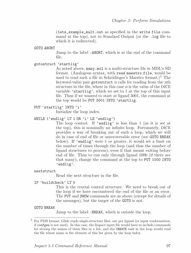
Chapter 3: Perform Simulations
(1ets_example_mult.out as specified in the write file com-mand at the top), not to Standard Output (or the .log file towhich it is redirected).
GOTO ABORTJump to the label :ABORT, which is at the end of the commandfile.
gotostruct ’startlig’As noted above, many.mol is a multi-structure file in MDL’s SDformat. (Analogous syntax, with read maestro file, would beused to read such a file in Schrodinger’s Maestro format.)3 Thekeyword-value pair gotostruct n calls for reading from the nthstructure in the file, where in this case n is the value of the DICEvariable ’startlig’, which we set to 1 at the top of this inputfile. Thus if we wanted to start at ligand 3001, the command atthe top would be PUT 3001 INTO ’startlig.
PUT ’startlig’ INTO ’i’Initialize the loop index.
WHILE (’endlig’ LT 1 OR ’i’ LE ’endlig’)The loop control. If ’endlig’ is less than 1 (as it is set atthe top), this is nominally an infinite loop. Fortunately, DICEprovides a way of breaking out of such a loop, which we willdo in case of end of file or unrecoverable error (see GOTO BREAKbelow). If ’endlig’ were 1 or greater, it would set a limit onthe number of times through the loop (and thus the number ofligand structures to process), even if that meant exiting beforeend of file. Thus to run only through ligand 1000 (if there arethat many), change the command at the top to PUT 1000 INTO’endlig’.
nextstructRead the next structure in the file.
IF ’buildcheck’ LT 0This is the crucial control structure. We need to break out ofthe loop if we have encountered the end of the file or an error.The PUT and SHOW commands are as above (except for details ofthe messages), but the target of the GOTO is not.
GOTO BREAKJump to the label :BREAK, which is outside the loop.
3 For PDB format, Glide reads single-structure files, one per ligand (or input conformation,if confgen is not used). In this case, the Impact input file would have to include commandsfor storing the names of these files in a list, and the CREATE task in the loop would readthe file whose name is the element of this list given by the loop index.
Impact 5.5 Command Reference Manual 97
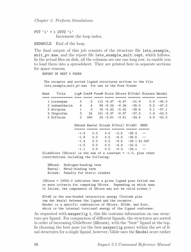
Chapter 3: Perform Simulations
PUT ’i’ + 1 INTO ’i’Increment the loop index.
ENDWHILE End of the loop.
The final output of this job consists of the structure file 1ets_example_mult_pv.mae, and the report file 1ets_example_mult.rept, which follows.In the actual files on disk, all the columns are one one long row, to enable youto load them into a spreadsheet. They are printed here in separate sectionsfor space reasons.
REPORT OF BEST 5 POSES
The receptor and sorted ligand structures written to the file
1ets_example_mult_pv.mae for use in the Pose Viewer
Rank Title Lig# Conf# Pose# Score GScore E(Cvdw) Eintern Emodel
==== ============ ==== ===== ===== ===== ====== ======= ======= ======
1 Lorazepam 5 2 112 -6.47 -6.47 -31.9 0.6 -45.3
2 indomethacin 4 4 84 -6.24 -6.24 -35.0 8.5 -47.2
3 Atropine 1 3 16 -5.42 -5.42 -38.8 2.1 -57.1
4 Ibuprofen 3 24 151 -5.37 -5.37 -27.3 1.8 -42.2
5 Diflucan 2 340 24 -3.61 -3.61 -34.4 4.9 -42.3
Ehbond Emetal Eclash E(Coul) E(vdW) RMSD
====== ====== ====== ======= ====== ======
-1.9 0.0 0.0 -2.5 -29.3 --
-1.9 0.0 0.0 -6.5 -28.5 --
-1.4 0.0 0.0 -9.6 -29.1 61.597
-1.5 0.0 0.0 -4.9 -22.4 --
-1.1 0.0 0.0 -5.3 -29.1 --
GlideScore (GScore) is the sum of a constant = -1.0, plus other
contributions including the following:
EHbond: Hydrogen-bonding term
Emetal: Metal-binding term
Eclash: Penalty for steric clashes
(GScore = 10000.0 indicates that a given ligand pose failed one
or more criteria for computing GScore. Depending on which ones
it failed, the components of GScore may not be valid either.)
ECvdW is the non-bonded interaction energy (Coulomb plus
van der Waals) between the ligand and the receptor.
Emodel is a specific combination of GScore, ECvdW, and Eint,
which is the internal torsional energy of the ligand conformer.
As requested with maxperlig 1, this file contains information on one struc-ture per ligand. For comparison of different ligands, the structures are sortedin order of increasing GlideScore (GScore), with the “best” ligand at the top.In choosing the best pose (or the best maxperlig poses) within the set of fi-nal structures for a single ligand, however, Glide uses the Emodel score rather
98 Impact 5.5 Command Reference Manual
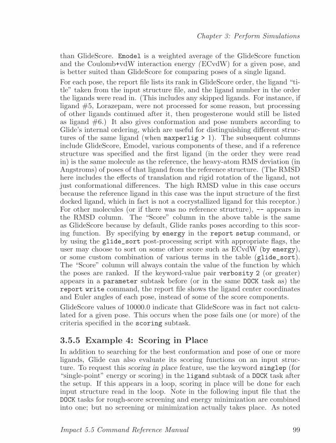
Chapter 3: Perform Simulations
than GlideScore. Emodel is a weighted average of the GlideScore functionand the Coulomb+vdW interaction energy (ECvdW) for a given pose, andis better suited than GlideScore for comparing poses of a single ligand.For each pose, the report file lists its rank in GlideScore order, the ligand “ti-tle” taken from the input structure file, and the ligand number in the orderthe ligands were read in. (This includes any skipped ligands. For instance, ifligand #5, Lorazepam, were not processed for some reason, but processingof other ligands continued after it, then progesterone would still be listedas ligand #6.) It also gives conformation and pose numbers according toGlide’s internal ordering, which are useful for distinguishing different struc-tures of the same ligand (when maxperlig > 1). The subsequent columnsinclude GlideScore, Emodel, various components of these, and if a referencestructure was specified and the first ligand (in the order they were readin) is the same molecule as the reference, the heavy-atom RMS deviation (inAngstroms) of poses of that ligand from the reference structure. (The RMSDhere includes the effects of translation and rigid rotation of the ligand, notjust conformational differences. The high RMSD value in this case occursbecause the reference ligand in this case was the input structure of the firstdocked ligand, which in fact is not a cocrystallized ligand for this receptor.)For other molecules (or if there was no reference structure), -- appears inthe RMSD column. The “Score” column in the above table is the sameas GlideScore because by default, Glide ranks poses according to this scor-ing function. By specifying by energy in the report setup command, orby using the glide_sort post-processing script with appropriate flags, theuser may choose to sort on some other score such as ECvdW (by energy),or some custom combination of various terms in the table (glide_sort).The “Score” column will always contain the value of the function by whichthe poses are ranked. If the keyword-value pair verbosity 2 (or greater)appears in a parameter subtask before (or in the same DOCK task as) thereport write command, the report file shows the ligand center coordinatesand Euler angles of each pose, instead of some of the score components.GlideScore values of 10000.0 indicate that GlideScore was in fact not calcu-lated for a given pose. This occurs when the pose fails one (or more) of thecriteria specified in the scoring subtask.
3.5.5 Example 4: Scoring in Place
In addition to searching for the best conformation and pose of one or moreligands, Glide can also evaluate its scoring functions on an input struc-ture. To request this scoring in place feature, use the keyword singlep (for“single-point” energy or scoring) in the ligand subtask of a DOCK task afterthe setup. If this appears in a loop, scoring in place will be done for eachinput structure read in the loop. Note in the following input file that theDOCK tasks for rough-score screening and energy minimization are combinedinto one; but no screening or minimization actually takes place. As noted
Impact 5.5 Command Reference Manual 99
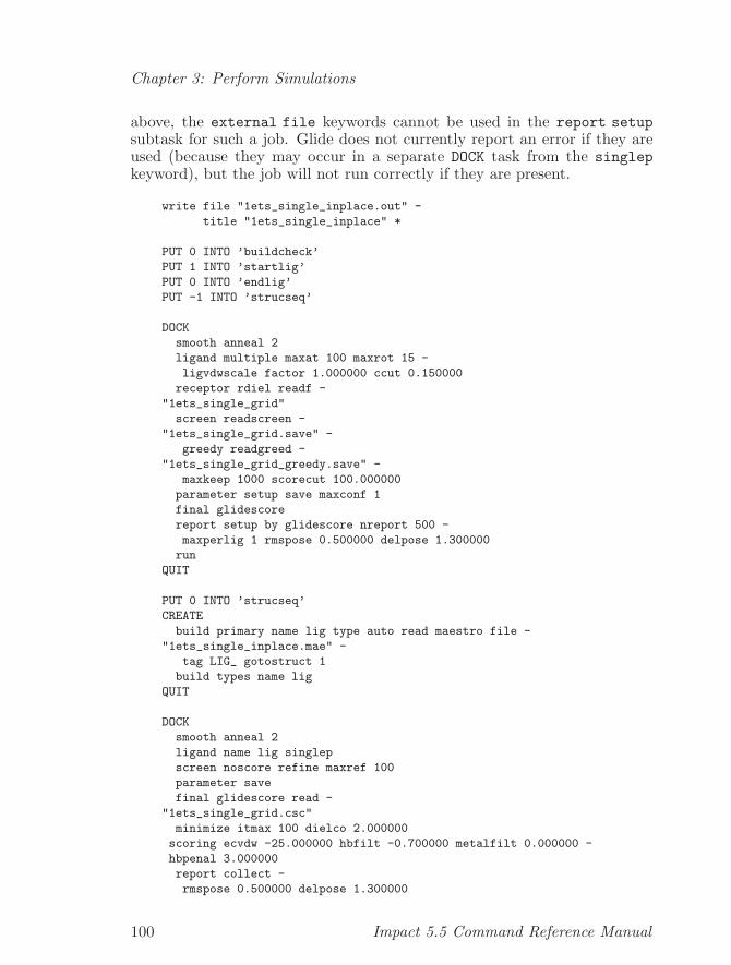
Chapter 3: Perform Simulations
above, the external file keywords cannot be used in the report setupsubtask for such a job. Glide does not currently report an error if they areused (because they may occur in a separate DOCK task from the singlepkeyword), but the job will not run correctly if they are present.
write file "1ets_single_inplace.out" -
title "1ets_single_inplace" *
PUT 0 INTO ’buildcheck’
PUT 1 INTO ’startlig’
PUT 0 INTO ’endlig’
PUT -1 INTO ’strucseq’
DOCK
smooth anneal 2
ligand multiple maxat 100 maxrot 15 -
ligvdwscale factor 1.000000 ccut 0.150000
receptor rdiel readf -
"1ets_single_grid"
screen readscreen -
"1ets_single_grid.save" -
greedy readgreed -
"1ets_single_grid_greedy.save" -
maxkeep 1000 scorecut 100.000000
parameter setup save maxconf 1
final glidescore
report setup by glidescore nreport 500 -
maxperlig 1 rmspose 0.500000 delpose 1.300000
run
QUIT
PUT 0 INTO ’strucseq’
CREATE
build primary name lig type auto read maestro file -
"1ets_single_inplace.mae" -
tag LIG_ gotostruct 1
build types name lig
QUIT
DOCK
smooth anneal 2
ligand name lig singlep
screen noscore refine maxref 100
parameter save
final glidescore read -
"1ets_single_grid.csc"
minimize itmax 100 dielco 2.000000
scoring ecvdw -25.000000 hbfilt -0.700000 metalfilt 0.000000 -
hbpenal 3.000000
report collect -
rmspose 0.500000 delpose 1.300000
100 Impact 5.5 Command Reference Manual
Chapter 3: Perform Simulations
run
QUIT
DOCK
parameter clean final
report -
rmspose 0.500000 delpose 1.300000 write filename -
"1ets_single_inplace"
run
QUIT
END
The output of a score-in-place job is written to a .scor file, in this case1ets_single_inplace.scor. This file gives the components of GlideScoreand ECvdW for each input ligand (in this case only one). There is nostructural output file (like the _pv.mae files in previous examples), becausethe structure is the same as in the input file.
-----------------------------------------------------------------------------
Lig # Title GScore HBond Metal Lipo RotB Clash BuryP ECvdW ECoul EvdW
1 -11.40 -4.55 0.00 -6.58 0.73 0.00 0.00 -70.01 -19.98 -50.03
-----------------------------------------------------------------------------
GlideScore (GScore) is the sum of a constant = -1.0, plus the
following contributions:
HBond: Hydrogen-bonding term
Metal: Metal-binding term
Lipo: Lipophilic contact term
RotB: Penalty for freezing rotatable bonds
Clash: Penalty for steric clashes
BuryP: Penalty for buried polar groups
(GScore = 10000.0 indicates that a given ligand pose failed one
or more criteria for computing GScore. Depending on which ones
it failed, the components of GScore may not be valid either.)
ECvdW is the non-bonded interaction energy (Coulomb plus
van der Waals) between the ligand and the receptor.
3.5.6 Example 5: Glide Constraints
Glide constraints are requirements that docked ligands have specific inter-actions with the receptor. During grid generation, you can define up to tenconstraints in the receptor, each of which may be a polar hydrogen atom,hydrogen-bond acceptor, or metal ion (atom-based constraint); a hydropho-bic region on and near the receptor surface (hydrophobic constraint); or thespherical region within a specified distance of a specified point (positionalconstraint). For atom-based constraints, if you specify a receptor atom that
Impact 5.5 Command Reference Manual 101
Chapter 3: Perform Simulations
is part of a functional group, and has a structural symmetry with one ormore other atoms of the same chemical type in the group, then Glide willautomatically include the symmetry-related atoms as part of the same con-straint specification, and will consider a ligand interaction with any one ofthem as satisfying the constraint.During ligand docking, you can specify that ligand poses must have appro-priate atoms in appropriate positions relative to up to four of these receptorconstraint sites, in order to be considered for docking. The categories of lig-and atoms that qualify to satisfy each constraint are specified by SMARTSpatterns in a feature file, which allows both restriction within and flexibil-ity beyond the atom types normally considered as participating in hydro-gen bonding, metal ligation, etc. For each hydrophobic constraint that youchoose to enforce, you can specify the minimum number of ligand hydropho-bic heavy atoms (default 1) that must lie in the corresponding hydrophobicregion around the receptor in order to satisfy the constraint.Because Glide incorporates any constraint specifications in several of its hi-erarchical filters (and incurs little additional computational cost in doingso), using constraints can accelerate docking calculations. This occurs be-cause large regions of pose space can be quickly eliminated (as well as entireligands that don’t have the right kind of atoms to satisfy the constraints),beyond what a given Glide filter would eliminate without the constraints.In addition, by eliminating “false positive” ligands or poses, constraints canimprove enrichment factors in database screening. And by restricting the al-lowed binding modes, judiciously chosen constraints may also improve dock-ing accuracy.As the following two examples demonstrate, you must specify constraints inthe receptor subtask of the initial DOCK task, in both the grid generation andligand docking jobs. The grid generation job needs to know which receptoratoms or regions you want to require ligand atoms to interact with. Inaddition, because hydrophobic constraints are not associated with individualatoms, a grid generation job needs to read a file containing a description ofthe hydrophobic regions (a list of the grid cells included in each region) thatdefine such constraints. The name of this file must be supplied explicitlyin the main input file; the Maestro interface calls the file base.phob, wherebase is the “base name” specified with the readf and writef keywords.For a positional constraint, you must specify the Cartesian coordinates of aposition, and the radius of the sphere around that position in which one ormore ligand atoms must lie to satisfy the constraint. The grid generationjob extracts or calculates information about the receptor atoms that definehydrogen-bond and metal constraints (such as their types and locations)that the docking job will use in enforcing the constraints, and writes theinformation to a file (default name base.cons), along with the grid cell listsit gets from the base.phob file for hydrophobic constraints, and those itcalculates from the sphere centers and radii for positional constraints. The
102 Impact 5.5 Command Reference Manual
Chapter 3: Perform Simulations
docking job needs to know that it must read the constraint definition file thatthe grid generation job wrote, and which of the constraints defined thereinit must enforce.
DOCK
smooth anneal 2
receptor rdiel name recep -
constraints ncons 4 nphobic 2 file "1kv2_grid.phob" -
consatom 1065 -
consatom 2531 -
writef "1kv2_grid" writerdiel -
protvdwscale factor 1.000000 ccut 0.250000 -
box center read xcent 4.700036 ycent 15.307946 zcent 33.614067 -
boxxrange 29.622122 boxyrange 29.622122 boxzrange 29.622122 -
actxrange 29.622122 actyrange 29.622122 actzrange 29.622122
screen greedy -
box center read xcent 4.700036 ycent 15.307946 zcent 33.614067 -
ligxrange 10.000000 ligyrange 10.000000 ligzrange 10.000000 -
writescreen "1kv2_grid.save" -
writegreed "1kv2_grid_greedy.save" -
maxkeep 5000 scorecut 100.000000
parameter clean
final glidescore
run
QUIT
In this grid generation job, we define four constraints (ncons 4) in the proteinkinase P38 (Protein Data Bank entry 1KV2). Two of the constraints arehydrophobic (nphobic 2), and the hydrophobic regions of interest are inthe file 1kv2_grid.phob, which the Maestro interface wrote (based on acalculation of a hydrophobic surface for the protein, and user selection ofdesired grid cells) in setting up the job. In this case, the regions correspondto the locations of naphthalene and tert-butyl moieties of the cocrystallizedligand in the 1KV2 structure. The other two constraints (the number is notexplicitly listed, but obviously equal to the difference between the nconsand nphobic values) are either hydrogen bonds or metal ions, in either casedefined by single protein atoms (and symmetry-equivalent ones, if any). Welist each of these atoms (consatom) by its atom index in the input structure.In this case, the atoms are the side-chain (carboxylate) oxygen(s) of residueGLU 71 and the backbone (amide) hydrogen of ASP 168; the cocrystallizedligand in the 1KV2 structure makes hydrogen bonds to both of these atoms,though not all known active ligands do.In a ligand docking job, you may specify up to four of the constraints definedin the previous gridgen job, for Glide to enforce when docking ligands. Thelisting of which constraints are eligible for enforcement, and the specificationof how many of those eligible are required to be satisfied, are contained inthe feature file, along with the specification for each listed constraint ofSMARTS patterns that ligand atoms must match in order to satisfy thatconstraint.
Impact 5.5 Command Reference Manual 103
Chapter 3: Perform Simulations
In the excerpt shown below from a ligand docking job, the receptor subtaskindicates that we want to apply constraints set up in a prior grid generationjob. The feature file 1kv2_dock_1cons.feat might list any number of thepreviously defined constraints (and SMARTS patterns to match ligand atomsthat can satisfy them), but specify that only some smaller number of them isrequired to be satisfied. For instance, if it lists three constraints and specifiesthat one is required, then ligands and poses that satisfy any one of thosethree constraints may appear in the output. If the grid generation job definedten constraints, then the feature file can in principle list all ten, but cannotspecify a number greater than four as the satisfaction requirement. For agiven set of grid files, different docking jobs will in general have differentfeature files associated with them.The keywords restcoef and restexp give parameters of a restraining po-tential that Glide uses to enforce the constraints during grid-energy opti-mization. This potential is a Gaussian function of the distance r betweena polar hydrogen and a hydrogen-bond acceptor, or a metal ion and its co-ordinating atom in the ligand, centered at the equilibrium distance for thegiven interaction:
V (r) = −A exp[−b (r − r0)
2]
where r0 is the equilibrium distance, 1.85A for a hydrogen bond or 2.11Afor a metal-ligand interaction. The default values for the coefficients A andb are those shown below for restcoef and restexp: A = 30.0kcal/mol andb = 0.3A −2. These values of the parameters have yielded good results in oursimulations, but we do not claim that they are the only reasonable values.
DOCK
...
receptor rdiel readf -
"1kv2_grid" -
constraints loosedock 2 featurefile -
"1kv2_dock_1cons.feat" -
consname -
"1kv2_grid.cons" -
restcoef 30.0 restexp 0.3
...
QUIT
3.5.7 Subtask Smooth
Request smoothing of energy functions used in constructing grids.• smooth [cwall val] [csoft val] [vsoft val]
[anneal [1|2]]
104 Impact 5.5 Command Reference Manual
Chapter 3: Perform Simulations
cwall, csoftSmoothing parameters for Coulomb energy.
vsoft Smoothing parameter for Lennard-Jones energy.
anneal Controls minimization on smoothed and/or unsmoothed energysurface.
Both smoothing functions work by evaluating the standard energy functionsfor two atoms at an effective distance that is positive when the actual dis-tance between the atoms is zero. For the Coulomb energy, the effectivedistance at an actual distance d is given by
ceff = sqrt[d * d + cwall * cwall * exp( - (d * d) / csoft)],
and for the Lennard-Jones energy, byveff = d + vwall * exp( - (d * d) / vsoft).
(Note that in each case, the wall parameter is the value of the effectiveradius at d = 0, and the soft parameter determines how rapidly the functionreverts to its unsmoothed value as d increases, with a larger parameter givinga slower (or “softer”) transition.)Note that vwall is not user-specifiable. Instead, for the contribution of agiven protein atom, Glide uses half of the Lennard-Jones σ parameter forthat atom. The default values for the other parameters are cwall = 2.0 A,and csoft = vsoft = 4.0 A2. All of the parameters must be positive num-bers; if the user specifies any negative, all are ignored, a warning is issued,and smoothing is not performed. In addition, if the softness parameters arebelow certain lower bounds, the resulting smoothed potential will have alocal maximum (for a repulsive potential) at some positive distance, and aspurious minimum rather than a maximum at zero distance. For Coulombsmoothing, the lower bound is csoft = cwall * cwall. For Lennard-Jones,since vwall varies with the protein atom type, we use a lower bound largeenough to accommodate the largest σ/2 in paramstd.dat (3.358 A for theCs+ ion, which gives a lower bound of vsoft = 2.075 A2). If the user spec-ifies a softness lower than the applicable lower bound, a warning is issuedand the parameter is reset to equal the lower bound.With the smoothing functions, Glide offers the option of annealing duringgrid-energy minimization. This involves starting the minimization on thepotential-energy surface defined by the smoothed functions, and graduallyshifting to the unsmoothed functions. The advantage of this procedure is toallow exploration of more regions of ligand pose and conformational spaceearly in the process (because the smoothed functions have lower barriers),while still ending at a minimum of the original grid potential rather thanat a pose whose energy is made artificially low by smoothing. Specifyingsmooth anneal 2 when calculating grids will result in both smoothed andunsmoothed functions being calculated (and saved to disk); the same specifi-cation in the task where minimization is done will result in annealing duringminimization. Smooth anneal 1 means calculate, save, and/or minimize on
Impact 5.5 Command Reference Manual 105
Chapter 3: Perform Simulations
only the smoothed surface. To calculate or minimize on only the unsmoothedpotentials, omit the smooth subtask entirely. We strongly recommend usingsmooth anneal 2 in all cases.
3.5.8 Subtask Receptor
Specify receptor molecule(s) and active site.• receptor [writef writebase] [readf readbase] -
[cdiel | rdiel | nil] -
[writecdie | writerdie | nil] -
[name spec [mole [mol | all]] -
[constraints [ncons num_cons -
[nphobic num_phob file fname] -
[nposit num_posit (xpos val ypos val zpos val -
rpos val constitle cons) repeated num posit times] -
(consatom num constitle cons) -
repeated (num cons − num phob − num posit) times] -
[consname file] [restcoef val][restexp val] -
[metalbind [charged | neutral | any]] -
[featurefile fname [featverb num] | -
nusecons num_ucons [nusephob num_uphob -
(usephob num nfill num) repeated num uphob times] -
(usecons num) repeated (num ucons − num uphob) times] -
[loosegrid num] [loosedock num] [finalonly]] -
[bsize size] [nlev nlevels] -
[(scut val) repeated nlevels-1 times] -
[box center read xcent val ycent val zcent val -
boxxr val boxyr val boxzr val -
actxr val actyr val actzr val] -
[active nsec num_sections -
(fres num lres num) repeated num sections times -
[buffer val]] [readsurface file] [writesurface file]
writefreadf Write/read energy grids (or fields) to/from disk files. writef
writes adaptive grid structure information to writebase.grd,Coulomb potential (constant dielectric) to writebase coul.fld,Coulomb potential (linear dielectric) to writebase coul2.fld, andLennard-Jones grids to writebase vdw.fld. readf reads the filesif they exist, and calculates the energy grids from scratch if theydon’t (and there is a receptor structure specified with the namekeyword). At least one of readf and writef should always bespecified. If both are specified, Impact reads whatever files arepresent, and calculates and writes those that aren’t. (If read-base and writebase are different, Impact reads from the formerand writes to the latter.) The files specified by readf should ofcourse have previously been written as a result of a writef in aprevious docking task.
106 Impact 5.5 Command Reference Manual
Chapter 3: Perform Simulations
cdielrdiel Specifies whether the Coulomb energy should be calculated as-
suming a constant dielectric (cdiel) or a dielectric linear inthe interatomic distance (rdiel). If neither is specified, thedefault is to use the constant dielectric. If both cdiel andrdiel are specified, rdiel wins, i.e., the linear dielectric is used.We recommend rdiel (and dielco 2.0 in the minimize sub-task), to account, however roughly, for solvent effects. Notethat these keywords affect which grid file is read, not the orig-inal calculation and writing of the grids, which is controlled bywritecdie/writerdie.
writecdiewriterdie
Specifies whether Coulomb grids are written to disk for the con-stant (writecdie) or linear distance-dependent (writerdie) di-electric model. If neither is specified, both grids are written. (Ifboth are specified, the one that comes last wins.) Because gridfiles are large and we recommend always using the linear dielec-tric, we also recommend using writerdie to save disk space.
namemole Specifies the Impact species that includes the receptor
molecule(s). If the species contains more than one molecule(apart from bound solvent), then the mole keyword is required,with either the name (mol) of a single molecule, or all toindicate all molecules in the species are included.
constraintsRequire ligand poses to make specified interactions with the re-ceptor. As noted above (see Section 3.5.6 [Constraints (Dock-ing)], page 101), the constraints keyword must appear in bothgrid generation and ligand docking jobs in order for constraintsto be used. The appearance of the following keywords dependson the type of job.
ncons This keyword appears in grid generation jobs, andthe value gives the total number of constraints (ofall types combined) defined.
nphobic num file fnameThe value num gives the number of hydrophobicconstraints defined in a grid generation job. Thefile fname contains lists of grid cells near the recep-tor that constitute the hydrophobic region for eachsuch constraint.
Impact 5.5 Command Reference Manual 107
Chapter 3: Perform Simulations
npositxposyposzposrpos Specification of positional constraints, which are re-
quirements that a ligand atom (whose desired chem-ical characteristics will be defined in the ligand dock-ing job) occupy a specifed (generally small) regionof space. The nposit value gives the number of suchconstraints, each of which is defined as a sphericalregion centered at the Cartesian coordinates givenby (xpos,ypos,zpos), with radius rpos.
consatom For each atom-based (H-bond or metal) constraintdefined in a grid generation job, this specificationlists the index of the constraint atom (or one of a setof symmetry-equivalent atoms) in the input receptorstructure file.
constitleAn ASCII label for each constraint. This is specifiedin the Glide input file for positional and atom-basedconstraints only. For hydrophobic constraints, Glidereads the title from the file listed with nphobic.
consname This may appear in either grid generation or liganddocking jobs. It specifies an alternative file name forwriting or reading information about the receptorconstraint atoms. The default is writefbase.consor readfbase.cons, whichever is present in the samereceptor subtask.
restcoefrestexp These may be specified in a ligand docking job.
They are the depth (multiplicative coefficient, with-out the negative sign) and inverse square half-width(coefficient of the exponent) in a Gaussian potentialfunction added to enforce the constraints during en-ergy minimization. For the form of the potential,See Section 3.5.6 [Constraints (Docking)], page 101.
featurefileGives the name of a “feature” file, which specifieswhich constraints must be satisfied in a ligand dock-ing job (including optional as well as required con-straints, in one or more groups with a “number re-quired” specified for each group). In addition tolisting the constraints (by title and index in the
108 Impact 5.5 Command Reference Manual
Chapter 3: Perform Simulations
consname file that the grid generation job wrote),this file specifies what type of ligand atoms (thosematching listed SMARTS patterns) will be acceptedas matching each constraint.
featverb This number is a “verbosity” parameter used bythe portions of Glide that read the feature file, andmatch ligand atoms against SMARTS patterns. Thedefault, equivalent to featverb 1, prints very littleinformation about the file and the matches, whereasfeatverb 4 gives a complete listing of which con-straints and patterns are listed in the file, and whichpatterns are matched by each ligand to be docked.
loosegridIncrease the distance tolerance (by num A) for con-sidering grid cells to be appropriate locations forconstraint-satisfying ligand atoms. Used in gridgeneration jobs only, not docking, and affects onlyatom-based (H-bond and metal) and positional con-straints, not hydrophobic. (The qualifying grid cellsfor hydrophobic constraints are always consideredto be those stored in the file associated with thenphobic keyword, no more and no less.) Default,or loosegrid 0, is to use the distance tolerancesbuilt into the algorithm for calculating the grid cells.Looser criteria may improve pose recovery (i.e., in-crease the likelihood of finding constraint-satisfyingposes for active ligands), possibly at the cost of adecrease in computational speed.
loosedockIncrease the tolerances (by num A) for distancematches used to determine constraint satisfactionduring the rough-score stage of the Glide funnel.Used in ligand docking jobs only. Default, orloosedock 0, is to use the distance tolerancesbuilt into the constraint algorithm. Loosercriteria may increase the likelihood of findingconstraint-satisfying poses for active ligands,possibly at the cost of a decrease in computationalspeed.
finalonlyWith this keyword, used in ligand docking jobs only,constraints are used only at the beginning of thedocking run to filter out ligands that lack appropri-
Impact 5.5 Command Reference Manual 109
Chapter 3: Perform Simulations
ate atoms to satisfy the constraints, and at the endto filter out final poses that do not satisfy them, notat any intermediate stages of the Glide funnel. Theoutput poses from a constraints finalonly run,for each ligand that contains appropriate atoms,are the best (by Emodel score) constraint-satisfyingposes of that ligand that would have emerged froman unconstrained docking job.
metalbind [DEPRECATED]This may appear in a ligand docking job. It speci-fies that any ligand atom that satisfies a constraintto bind a metal ion in the receptor must bear anonzero formal charge (charged), must bear zeroformal charge (neutral), or may be in any formalcharge state (any). The default, and the recom-mended value, is charged.
nusecons [DEPRECATED]This and the following keywords may appear in aligand docking job, to select constraints to enforcefrom among those defined in the consname file thatthe grid generation job wrote. The nusecons valuegives the total number of constraints to enforce, ofall types.
nusephob [DEPRECATED]This gives the total number of hydrophobic con-straints to enforce.
usephob [DEPRECATED]nfill [DEPRECATED]
For each selected hydrophobic constraint, theusephob value gives its position in the consnamefile, and nfill the number of ligand hydrophobicheavy atoms that must be located in thecorresponding hydrophobic region.
usecons [DEPRECATED]These values are the positions of the selected non-hydrophobic constraints in the consname file. Notethat hydrophobic constraints are listed first in thisfile, so if there are two hydrophobic constraints,the “first” non-hydrophobic one is selected usingusecons 3.
bsize The size of the finest grid spacing for the energy grids, inAngstroms. Default 0.4.
110 Impact 5.5 Command Reference Manual
Chapter 3: Perform Simulations
nlev Number of levels of the adaptive grid. At each successive level(farther from the receptor surface), the grid spacing is twicewhat it is at the previous level. Thus if the smallest grid spacingis size, then the largest is 2(nlevels−1) * size. Default nlevels = 4.
scut Distances from the receptor (the closest receptor surface point)at which the grid spacing changes. Thus
bsize 0.4 nlev 2 scut 1.0
means that the grid spacing is 0.4 A for points closer than 1.0 Afrom the receptor surface, and 0.8 A farther away. If there ismore than one scut value (i.e., if nlevels > 2), they must begiven in descending order. The default (corresponding to bsize0.4 nlev 4) is scut 4.4 scut 2.8 scut 2.0.
box Explicitly specify the rectangular box in which the energy gridis defined, rather than building it based on a specification ofactive site residues.center read
Gives the three Cartesian coordinates of the cen-ter of the box, as the the numbers following xcent,ycent, and zcent. The keyword read is requiredhere because another option is available with thecenter keyword in the screen subtask, and thesame code is used to parse the box input in bothsubtasks.
boxxrboxyrboxzr The size of the grid box (in Angstroms) in the x,
y, and z directions. That is, the x-coordinates ofthe grid points in the box range from approximatelyxcent − boxxr/2 to xcent + boxxr/2. This is ap-proximate because extra space may be added to theends of the box so that it contains a whole numberof elementary cubes of the grid.
actxractyractzr Dimensions (Angstroms) of the box used to deter-
mine “active” residues whose surface is used in earlyrough-score filters. Surface points are calculated forall residues that have any atom in this box. In gen-eral this should be the same size as the grid box, butmemory limitations in the surface-generation algo-rithm require a box no larger than 50 A on a side.
active An alternative method of defining the dimensions of the gridand “active surface” boxes. Specifies which residues are to be
Impact 5.5 Command Reference Manual 111
Chapter 3: Perform Simulations
considered the active site of the receptor. The grid box is com-puted using the largest and smallest x-, y-, and z-coordinates ofatoms in these residues, and adding a distance in each direction(positive and negative) as specified with the buffer keyword.As when directly specifying actxr, etc., surface points are actu-ally generated for all residues with any atom in the box, not justthe ones specified here. The initial active residues are specifiedas num sections ranges, each given by a fres lres pair. Eachfres value must be greater than the previous lres (the firstmust be greater than zero), and each lres must be greater thanor equal to the corresponding fres (with equality implying arange consisting of a single residue). The maximum value ofnum sections is 100. (If you need more than that, consider fill-ing in to combine several ranges into one.) If neither active norbox is present, then all residues of the receptor are consideredto be in the active site, with a buffer of the default size, 11.0Angstroms.
nsec Indicates that the active site residues are given by the followingfres num1 lres num2 pairs, where each of the num sectionspairs indicates that all residues in the range num1 throughnum2, inclusive, are part of the active site. (Note that sucha “range” may consist of a single residue, as fres 79 lres 79.)
buffer Indicates that the box in which the grids are defined extends adistance bufval Angstroms beyond the minimal box that enclosesthe active site, in each of the positive and negative x, y, and zdirections. Default is 11.0.
readsurfacewritesurface
Read/write receptor surface points from/to the indicated file.The surface points are calculated from the positions and radii ofreceptor atoms in residues contained in the “active” box definedby either actxr, etc., or active, and are used in early filtersin the rough-score screening step. The surface calculation issomewhat time-consuming, so it may be convenient to store thepoints for future use, particularly in runs where the energy gridsare not being recalculated (which takes a much longer time) butthe rough-score grids are (which is quite fast, so recalculatingthe surface can add significantly to it).
3.5.9 Subtask Ligand
Specify ligand molecule.• ligand keep
• ligand multiple maxat nat [maxrot nbond] -
112 Impact 5.5 Command Reference Manual
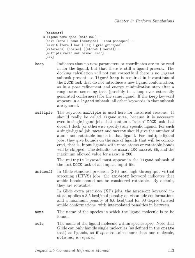
Chapter 3: Perform Simulations
[amideoff]
• ligand name spec [mole mol] -
[init [zero | rand [randopts] | read posespec] -
[cminit [zero | box | lig | grid gridspec] -
[reference] [noelec] [[stdrot | norot]] -
[multiple maxat nat maxmol nmol] -
[new]
keep Indicates that no new parameters or coordinates are to be readin for the ligand, but that there is still a ligand present. Thedocking calculation will not run correctly if there is no ligandsubtask present, so ligand keep is required in invocations ofthe DOCK task that do not introduce a new ligand conformation,as in a pose refinement and energy minimization step after arough-score screening task (possibly in a loop over externallygenerated conformers) for the same ligand. If the keep keywordappears in a ligand subtask, all other keywords in that subtaskare ignored.
multiple The keyword multiple is used here for historical reasons. Itshould really be called ligand size, because it is necessaryeven in single-ligand jobs that contain a “setup” DOCK task thatdoesn’t dock (or otherwise specify) any specific ligand. For sucha single-ligand job, maxat and maxrot should give the number ofatoms and rotatable bonds in that ligand. For multiple-ligandjobs, they give bounds on the size of ligands that will be consid-ered, that is, input ligands with more atoms or rotatable bondswill be skipped. The defaults are maxat 100 maxrot 35, and themaximum allowed value for maxat is 200.The multiple keyword must appear in the ligand subtask ofthe first DOCK task of an Impact input file.
amideoff In Glide standard precision (SP) and high throughput virtualscreening (HTVS) jobs, the amideoff keyword indicates thatamide bonds should not be considered rotatable. By default,they are rotatable.In Glide extra precision (XP) jobs, the amideoff keyword in-stead applies a 3.5 kcal/mol penalty on cis-amide conformationsand a maximum penalty of 6.0 kcal/mol for 90 degree twistedamide conformations, with interpolated penalties in between.
name The name of the species in which the ligand molecule is to befound.
mole The name of the ligand molecule within species spec. Note thatGlide can only handle single molecules (as defined in the createtask) as ligands, so if spec contains more than one molecule,mole mol is required.
Impact 5.5 Command Reference Manual 113
Chapter 3: Perform Simulations
referenceSpecifies that the current ligand molecule (the one most re-cently read in to the specified species) is to be taken as thereference conformation for root-mean-square deviation (rmsd)calculations. Such calculations are only meaningful, and Glideonly does them, for ligands that are the same molecule as thereference. Glide also issues a warning that rmsd calculationsmay not be meaningful for a multiple-ligand job, but the rmsdsit does calculate should be correct. In general (and in jobs setup and/or launched from the Maestro user interface), no actualdocking calculations are done in the DOCK task that specifies thereference ligand. It is of course possible to include the referenceligand in a subsequent DOCK task that actually does dock it.
initcminit Specify the initial pose of the ligand for energy minimization, if
rough-score screening is not performed. The usual specificationof these keywords (and the default) is init zero cminit lig.If rough-score screening is run, these keywords are ignored, be-cause the initial poses for minimization are those that survivescreening.
init zero Specifies that the ligand center should start at theorigin of coordinates, unless displaced by cminit.
init rand [cmrange val] [thetarange val] [phirangeval] [psirange val] [seed num]
Specifies a random starting pose. This is chosenin the ranges given with the keywords cmrange,thetarange, phirange, and psirange. Thatis, each Cartesian coordinate of the centerposition starts in the range (-cmrange/2) to(cmrange/2) Angstroms about the positionspecified by cminit; the Euler angle θ starts inthe range 0 to (thetarange) degrees; φ starts inthe range (-phirange/2) to (phirange/2), andsimilarly for ψ. iseed is a seed for the randomnumber generator. The defaults are cmrange 2.0thetarange 30.0 phirange 60.0 psirange 60.0iseed 137.
init read xcm val ycm val zcm val phi val theta val psival
Initializes the ligand to the specified pose (centercoordinates in Ansgtroms, angles in degrees), againsubject to modification by cminit.
114 Impact 5.5 Command Reference Manual
Chapter 3: Perform Simulations
cminit zeroSpecifies that the starting position of the ligand cen-ter should be at the origin, or unmodified from theposition specified by init. Thus specifying cminitzero with init zero or init rand would indeedplace the ligand at the origin of coordinates, or ran-domly in the specified range around it, which is un-likely to be useful. But cminit zero is the defaultwith init read, in which case it leaves the ligandat the specified position.
cminit ligStarts the ligand at the position given in the inputfile. This is the default with init zero and initrand. In the latter case, the starting position israndomly displaced in the specified range about theinput position.
noelec Turn off electrostatic interactions, by setting partial charges tozero for all atoms in the current ligand. This is reset for eachligand structure read in, so the noelec keyword must appear inthe first DOCK subtask for each ligand, e.g. in the ligand loop.Note also that the final reported Coulomb energy for a ligandpose is a “scaled” energy that depends on formal charges as wellas partial charges, and noelec does not zero the formal charges,so the output files (.rept and .mae) may report nonzero Coulombenergies even if noelec is set. But noelec does guarantee thatno electrostatic interactions are included in the sampling andenergy minimization steps, in which the final poses are produced.
stdrotnorot Control the starting orientation of the ligand. stdrot places the
ligand in a standard orientation, with its diameter (the line seg-ment connecting the two most widely separated ligand atoms)pointing along the z-axis. norot leaves the ligand in the ori-entation specified with the init keyword. With init read ...cminit zero, the ligand starts in the user-specified position andorientation, and the default is norot to leave it there. In allother cases, the default is stdrot. The Euler angles that de-fine poses, in both phases of the docking calculation, are thendefined relative to the standard orientation.
new Indicates that the current ligand molecule has a distinct struc-ture (not just a different conformation) from the preceding one.This keyword is usually unnecessary, because the newness of theligand is perceived automatically by build primary check in itsCREATE task.
Impact 5.5 Command Reference Manual 115
Chapter 3: Perform Simulations
3.5.10 Subtask Parameter
Specify various parameters and flags.• parameter [verbosity num] [maxconf num] -
[setup] [save] [clean]
This subtask sets certain controls on the overall operation of the task.
verbosityControls the amount of information printed to STDOUT andto the main output file. The default is verbosity 1, whichshould be sufficient for most users’ purposes. Certain things areprinted independent of the value of this parameter, including thesummary (labeled DOCKING RESULTS) of the best-scoring poses(by various criteria) for each ligand and their scores. verbosity0 (or less, which is equivalent to 0), prints a bare minimum ofadditional information. Values higher than 2 or 3, and especiallyhigher than 5, print information that’s very unlikely to be usefulto anyone other than developers and debuggers, and can resultin extremely large output files. A given verbosity level remainsin effect unless and until the parameter subtask of a subsequentDOCK task changes it.
maxconf The maximum number of ligand conformations to be processedin this job. This parameter sets the size of a dynamically allo-cated array, and attempting to read conformations beyond thisnumber will result in an error.
setup Indicates that the current invocation of the DOCK task is onlyfor the purpose of setting up arrays (including rough-score andenergy grids) for use by subsequent invocations in the same Im-pact job (as in multi-conformation loops). Though there willin general be a screen subtask along with parameter setup toset parameters for the rough-score screening, no actual screen-ing calculation on the ligand will actually be done at this point.(Nor will minimization, which there’s no reason to specify at allin a task with parameter setup.)
saveclean Specify the disposition of various dynamically allocated arrays
(including those that hold the rough-score grids, and the ligandand receptor coordinates copied from the main Impact arrays)at the end of the current invocation of the DOCK task. savemeans leave them in place for use by subsequent invocations ofthe task, clean means delete them, which means any subsequentinvocations must build them again. If setup is specified, saveis the default. (Indeed, setup clean doesn’t make sense: set upthe grids, don’t use them, and then throw them away.) If neithersetup nor save is specified, clean is the default. (But it doesn’t
116 Impact 5.5 Command Reference Manual
Chapter 3: Perform Simulations
hurt to specify save or clean, where appropriate, even if it isthe default.)
3.5.11 Subtask Confgen
Request internal generation of ligand conformers.• confgen -
ecut val [baddist val] -
[maxcore num] [corescale val] -
[noringconf]
This is the recommended method of incorporating ligand flexibility intoGlide, especially in a multi-ligand job. As shown in the examples above, thecommand sequence in an Impact input file should be different depending onwhether there is one input structure per ligand, with confgen specified, ormultiple structures assumed to be externally generated conformers for eachligand. In the latter case, we recommend a loop over screen subtasks, to runthe first stages of rough-score screening (through greedy score evaluation)on all of the conformers of a given ligand, before running pose refinement,grid-energy optimization, and final (GlideScore) scoring on all poses thatpass the first stages for that ligand. With confgen, by contrast, the loopover the internally generated conformations is specified by a single screensubtask, so the subsequent steps should ensue immediately.By default, confgen generates alternative ring conformations for five andsix membered non-aromatic rings. To turn off this procedure, use thenoringconf keyword. For six membered rings, the alternative chair confor-mation is generated if the equatorial–axial conformational change of the sub-stituents is empirically not too energetically costly. The five membered ringscurrently treated are sugar rings and five membered rings with N and/or Satoms. The alternative sugar ring conformation generated from the inputconsists of the energetically preferred pseudorotation. Five membered ringswith N or S atoms have a second ring conformation generated by rotationof the out-of-plane corner.
ecut This parameter is the energy cutoff used in the gas phase con-formation generation. Conformations with an energy above ecutrelative to the lowest energy conformation are not considered.Note that the energy scale here is with respect to the modeltorsion/1-4 vdW confgen potential and not a full force field po-tential.
baddist The baddist parameter is used to generate a pair list for in-tra ligand repulsion terms used in the gas phase generation ofconformations. We do not recommend changing this parameterfrom its default value of 2.45 A.
maxcore The maxcore parameter allows the user to define a maximumnumber of core conformations to be generated. The default be-
Impact 5.5 Command Reference Manual 117
Chapter 3: Perform Simulations
havior is to use a functional form depending on the number ofrotatable bonds. The maxcore parameter could be used to makea very approximate rough quick pass at docking. See Section 2of the Glide Technical Notes for details.
corescaleCorescale is a fractional value to scale down the default numberof core conformations kept. See Section 2 of the Glide TechnicalNotes.
noringconfThe noringconf keyword disables ring conformation generation.
3.5.12 Subtask Similarity
Request Glide similarity scoring.Similarity scoring entails assigning a number to each ligand based on itssimilarity to one or more of a set of selected active ligands, and optionally(weighted or calibrated similarity) also its dissimilarity to a set of selectedinactive or decoy ligands. Unlike most quantities calculated in Glide, sim-ilarity is a ligand-based rather than a structure-based property. That is,the similarity between two molecules depends only on the types and con-nectivity of the atoms in those molecules, and not on any details of theircoordinates or conformations, or on anything to do with the receptor. Glidethus performs similarity scoring, if requested, just once per ligand. It there-fore adds negligible overhead to a typical Glide database screening job, andmay even speed it up because some ligands can be immediately rejected.Weight calibration adds a small amount of time to a grid generation job.The similarity of one ligand (in the test set) to another (in the training set) isevaluated by comparing the set of all atom pairs in the test ligand to the setof all atom pairs in the training ligand. Within each ligand, each atom pairis characterized by the element types, bond orders, and formal charges of thetwo atoms, and the number of bonds in the shortest path connecting them.The similarity is normalized to a number between 0 (the two molecules haveno atom pairs in common) and 1, in which case the molecules have all thesame atoms with the same connectivities, and are thus either identical orstereoisomers of each other. For weighted similarity, each atom pair in thetraining set (actives) is assigned a weight factor, which is higher if the givenpair appears more often in the actives and lower if it appears in the inactives.To use similarity scoring, put simil subtasks in the grid generation (only forcalibration in weighted similarity) and ligand docking tasks, following themeta-examples below. Glide will then adjust the Glidescore of each dockedligand pose by adding a term that depends on the maximum similarity ofthat ligand to any of the actives.
• simil weight actives [maestro | sd] afile fname -
inactives [maestro | sd] ifile fname -
118 Impact 5.5 Command Reference Manual
Chapter 3: Perform Simulations
percent val wfile fname [allprint | noprint]
• simil actives [maestro | sd] afile fname -
[wfile fname] -
[penalty val] [lowsim val] -
[highsim val] [reject val] [allprint | noprint]
• simil name spec
The calibration step for weighted similarity is specified by the weight key-word. This step should be performed in a grid generation job, and all of thefollowing keywords are required.
actives [maestro | sd] afile fnameSpecifies that the active ligands in the training set are in filefname, which may be in either Maestro or MDL SD format.Note that at least two active ligands are required for calibration.
inactives [maestro | sd] ifile fnameSpecifies the file containing the decoy ligands.
percent valRoughly specifies the percentage of the inactives to be includedin weight calibration. Rather than using preselected ligandsfrom the inactives file, each molecule in the file has val percentprobability of being used in weight calibration. Thus, the num-ber of ligands selected may not exactly match the user’s percentinput. Note that at least one decoy compound is required forcalibration, and that a weight calibration job will exit if it hasnot read in at least two active ligand structures, and chosenat least one inactive. For best results, we recommend makingthe inactives file large enough, and the percent probabilityhigh enough, to use about 5 to 15 times as many decoys as ac-tives. For instance, if the actives file contains 10 ligands andthe inactives file contains 1000, use a percent value between5.0 and 15.0. Weight calibration may produce a message statingthat it did not converge (more likely the higher the ratio of inac-tives to actives), but this is not a problem: a valid weights file isproduced in any case, and contains the "best" weights obtainedwith the given structures.
wfile fnameWrite the weights to the file fname. This will be a text file, witheach line containing a symbolic representation of an atom pair,followed by the calibrated weight for that pair.
allprint The allprint keyword enables maximum printing of outputfrom the similarity machinery including output of the similarityof each docked ligand to each probe molecule. Default printingoutputs only the maximum simiarity of the docked ligand to anyprobe molecule.
Impact 5.5 Command Reference Manual 119
Chapter 3: Perform Simulations
noprint The keyword noprint disables printing of output from the sim-ilarity machinery.
To use similarity scoring in a ligand docking job, all that’s required is thespecification of an actives file. The simil subtask should appear in thefirst (setup) DOCK task of the job.
actives [maestro | sd] afile fnameAdjust the Glidescore values for poses of each ligand accordingto the similarity of that ligand to those in file fname. This neednot be the same file as was used for weight calibration in theprevious grid generation job, even if the weights generated inthat job are to be used.
wfile fnameUse calibrated similarity, with weights taken from file fname.
penalty val lowsim val highsim valParameters for adjusting Glidescores. If the maximum similaritybetween a given docked ligand and any ligand in the actives fileis less than lowsim, add the full penalty value to the Glidescoresof all docked poses of that ligand. If the maximum similarity isgreater than highsim, do not adjust the Glidescores for thatligand. If the maximum similarity is between those two values,the Glidescore adjustment is determined by a linear ramp be-tween the maximum penalty value and zero. Note that whilelowsim must be less than or equal to highsim, there are noother restrictions on their values; in particular, they need notbe between 0.0 and 1.0, even though all similarity scores will bein that interval. Choosing lowsim less than zero, for instance,simply means that the maximum penalty value will never beapplied to any ligand. Also, penalty may be negative, in orderto reward ligands that are not similar to any of the actives (topromote diversity, for instance). The defaults are penalty 6.0lowsim 0.3 highsim 0.7.
reject valSkip any ligand whose maximum similarity to any active ligandis less than val. Must be between 0.0 (accept all ligands) and1.0 (skip all ligands that are not identical to or stereoisomers ofone of the actives). Default is reject 0.0.
The third form of the simil command, simil name spec , should appear inthe DOCK task for each ligand. (The first for that ligand, with ligand namespec rather than ligand keep.) It simply indicates that similarity scoringis to be applied to species spec (the current ligand), using the actives file(and weights, if any) read in the initial (setup) DOCK task.
120 Impact 5.5 Command Reference Manual
Chapter 3: Perform Simulations
3.5.13 Subtask Screen
Request screening phase of docking calculation.• screen noscore -
[refine [refstep num] [maxref num] [refgreedy]]
• screen [scbsize val] [skipb num] -
[maxkeep num] [scorecut val] -
[readscreen fname] [writescreen fname] -
[box center -
[lig | read xcent val ycent val zcent val] -
[boxxr val boxyr val boxzr val] -
[ligxr val ligyr val ligzr val]] -
[readcmsite fname] [writecmsite fname] -
[greedy [fraction weight] [readgreed fname] -
[writegreed fname]] -
[refine [refstep num] [maxref num] [refgreedy]]
noscore Do not perform rough-score calculations or screening on the cur-rent ligand. This keyword is needed when the refine step mustbe performed after a loop (either in DICE or internally) has al-ready done screening on multiple (internally or externally gen-erated) conformations. It is probably not useful otherwise.
scbsize The grid spacing, in Angstroms, of the rough-score grid. Defaultis scbsize 1.0.
skipb n Use only every n’th grid point in each direction as a possible sitefor the ligand center. Thus skipb 2, the default uses one-eighthof all grid points.
maxkeep Maximum number of poses to pass to the grid energy calculation.Default is maxkeep 1, but it’s generally not useful to leave it atthat. In our tests, we have found that a few hundred poses, overmultiple conformations, are usually enough to find one or moregood docked poses, at least if greedy scoring and pose refinementare employed.
scorecut Rough-score cutoff for keeping poses. When accumulating posesto pass to the grid energy calculations (after they have passedall other screening tests), a given pose survives if its rough scoreis within scorecut of the best pose accumulated so far. Defaultis scorecut 100.0.
readscreenwritescreen
Read/write the rough-score grids (and possibly other informa-tion: see readcmsite below) from/to the indicated file. The filespecified in a readscreen should have been written as the resultof a writescreen in a previous run with the same receptor.
Impact 5.5 Command Reference Manual 121
Chapter 3: Perform Simulations
writecmsiteWrite to disk information about possible grid sites for the ligandcenter, for those sites that pass an initial (ligand-independent)filter. This is generally a much smaller set than the entire boxwhere the rough-score grid is defined, so Glide calculates it oncefor a given receptor and store the list on disk for subsequent usewith different ligands. If writecmsite is not specified, this in-formation is appended to the file specified in writescreen. Dif-ferent box specifications, or different skipb specifications, resultin different lists of sites, so we provide the option of writing theseto separate files, without repeating the much larger rough-scoregrids in the writescreen file, which are independent of skipb.
box Specifies the rectangular box where the rough-score function isdefined (enclosing box), and/or narrower limits on the positionof the ligand center (bounding box). Default for the enclosingbox is that specified in the receptor subtask for the energygrids, either by the active and buffer specifications or by abox specification in that subtask. The box center and boxxrspecifications are as in the receptor subtask, with the addi-tional option box center lig to put the center of the box atthe coordinates of the ligand center in the input file. If theinput is a known co-crystallized complex, box center lig bi-ases the calculation in favor of the known correct answer, andshould not be used except for testing. The parameters ligxr,ligyr, and ligzr give the size of the search space for posi-tions of the ligand center. That is, the ligand center may beplaced at grid points with x-coordinates between approximatelyxcent−ligxr/2 and xcent+ligxr/2, and similarly for y and z.In general, the bounding box should be much smaller than theenclosing box, because grid points near the edges of the enclos-ing box will have many ligand atoms outside the box, and thusbe rejected as possible ligand center positions. The Maestro userinterface determines the size of the enclosing box (purple outlineon the Maestro display) by adding to the user-specified size ofthe bounding box (green) a buffer big enough to fit ligands upto a user-specified size, when the ligand center is at the edges orcorners of the bounding box. The limits on the ligand center po-sition are incorporated in the grid file written by writescreen(or writecmsite), so box ... ligxr ... is unnecessary whenreading existing grid files from disk readscreen.
greedy Specifies the greedy scoring algorithm, as described above.fraction weight specifies that the combination to use is weighttimes the score at the best surrounding grid point, plus (1 −weight) times the original score at the central point. The de-
122 Impact 5.5 Command Reference Manual
Chapter 3: Perform Simulations
fault is fraction 0.33, and acceptable values are between 0and 1. readgreed and writegreed specify reading/writing thegreedy grid (the linear combination at each point, not the bestsurrounding score) from/to the indicated file.
refine Specifies the pose refinement step of the screening algorithm.This involves moving each pose from its original central gridpoint to a 3 x 3 cube of surrounding grid points. Each pointis either zero or refstep grid points away from the centralone in each of the positive or negative x, y, and z directions,where refstep must be smaller than skipb (so as not to getto a position already tested for the ligand center), and the de-fault is refstep 1. The algorithm evaluates the score of thepose centered at each of the 27 grid points (in the same orien-tation as the original), and chooses the best (lowest) score topass to energy minimization. The refinement step improves thescores of poses that are close to favorable ones that were ini-tially skipped because of the skipb specification, and thus oftendecreases the number of poses that need to be passed to energyminimization in order to assure that good ones are included. Todecrease the number actually passed, specify maxref less thanmaxkeep. Since pose refinement and greedy scoring are bothintended to find good scores that would otherwise be missedbecause of skipb, the default is for refinement to evaluate the27 poses using the original (non-greedy) score, even if the restof the screening process used the greedy score. The keywordrefgreed specifies that refinement should use greedy scoring (ifthe greedy-score grid is available), but we have not found anyadvantage in doing this, and it runs the risk of increasing therate of false positives.
3.5.14 Subtask Minimize
Request energy minimization phase of docking calculation.• minimize flex ftol val dielco val -
[ maxhard val ] [ maxsoft [val] [ sampling val ] -
[ highacc [ ncycle val ] ]
flex Indicates that ligand torsional angles are to be varied duringminimization.
ftol Convergence criterion for the minimizer, expressed as a boundon the relative energy change at the last iteration. The defaultis ftol 1.0e-4.
dielco The dielectric constant, or coefficient of the interatomic dis-tance in the distance-dependent dielectric function, to be usedin calculating electrostatic energies. Thus if rdiel is specified
Impact 5.5 Command Reference Manual 123
Chapter 3: Perform Simulations
in the receptor subtask, and dielco 2.0 is specified here, thedielectric used is 2r. The default is dielco 1.0, but we recom-mend (and the Maestro interface writes) dielco 2.0, along withrdiel, to weaken long-range electrostatic interactions.
sampling The value of this keyword controls the sampling of ligand tor-sions, performed after minimization and before final scoring.Lower values indicate more sampling. The default, sampling-1, does the most sampling, and sampling 10 does no post-minimization sampling. In general, more sampling results inbetter-docked and better-scoring poses, at the cost of increasedcomputation time.
maxhard The maximum number of minimization iterations on the hardCoulomb-vdW surface, default is 50.
maxsoft The maximum number of minimization iterations on the softCoulomb-vdW surface, default is 100.
highacc This keyword activates Glide’s extra precision mode, it directlycorresponds to choosing “Extra Precision” in the Maestro Glidepanel “Choose Docking Mode” pull-down selector.
ncycle valThis keyword is only available when highacc is also used, andsets the number of times the ligands are recycled through thedocking process. This additional effort greatly improves Glide’sability to sample all the docking positions of the ligand in thereceptor grid. The default value is 5.
3.5.15 Subtask Final
Specify final scoring function.• final [glidescore|noglidescore] [read fname]
The final subtask specifies the scoring function to be used for final eval-uation of the docking affinity of ligand poses. The recommended scoringfunction is Schrodinger’s proprietary GlideScore (tm). final glidescoreshould appear in the setup DOCK task, and in cases where receptor infor-mation is to be read from disk, the keyword-value pair read fname shouldappear in the DOCK tasks that do the scoring, to indicate the file that con-tains receptor information needed for calculating GlideScore. In general, thename of this file will be gridjob.csc, where gridjob is the name of the jobin which receptor grids were created.
3.5.16 Subtask ScoringFilters and parameters for final scoring.
scoring ecvdw val hbfilt val metalfilt val -
hbpenal val
124 Impact 5.5 Command Reference Manual
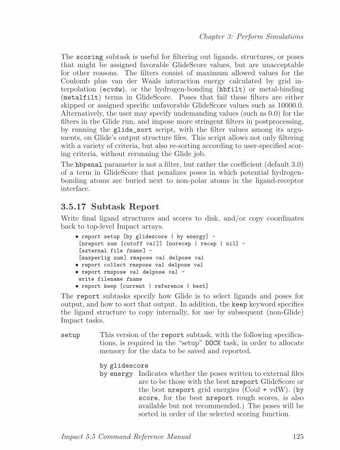
Chapter 3: Perform Simulations
The scoring subtask is useful for filtering out ligands, structures, or posesthat might be assigned favorable GlideScore values, but are unacceptablefor other reasons. The filters consist of maximum allowed values for theCoulomb plus van der Waals interaction energy calculated by grid in-terpolation (ecvdw), or the hydrogen-bonding (hbfilt) or metal-binding(metalfilt) terms in GlideScore. Poses that fail these filters are eitherskipped or assigned specific unfavorable GlideScore values such as 10000.0.Alternatively, the user may specify undemanding values (such as 0.0) for thefilters in the Glide run, and impose more stringent filters in postprocessing,by running the glide_sort script, with the filter values among its argu-ments, on Glide’s output structure files. This script allows not only filteringwith a variety of criteria, but also re-sorting according to user-specified scor-ing criteria, without rerunning the Glide job.The hbpenal parameter is not a filter, but rather the coefficient (default 3.0)of a term in GlideScore that penalizes poses in which potential hydrogen-bonding atoms are buried next to non-polar atoms in the ligand-receptorinterface.
3.5.17 Subtask Report
Write final ligand structures and scores to disk, and/or copy coordinatesback to top-level Impact arrays.
• report setup [by glidescore | by energy] -
[nreport num [cutoff val]] [norecep | recep | nil] -
[external file fname] -
[maxperlig num] rmspose val delpose val
• report collect rmspose val delpose val
• report rmspose val delpose val -
write filename fname
• report keep [current | reference | best]
The report subtasks specify how Glide is to select ligands and poses foroutput, and how to sort that output. In addition, the keep keyword specifiesthe ligand structure to copy internally, for use by subsequent (non-Glide)Impact tasks.
setup This version of the report subtask, with the following specifica-tions, is required in the “setup” DOCK task, in order to allocatememory for the data to be saved and reported.
by glidescoreby energy Indicates whether the poses written to external files
are to be those with the best nreport GlideScore orthe best nreport grid energies (Coul + vdW). (byscore, for the best nreport rough scores, is alsoavailable but not recommended.) The poses will besorted in order of the selected scoring function.
Impact 5.5 Command Reference Manual 125
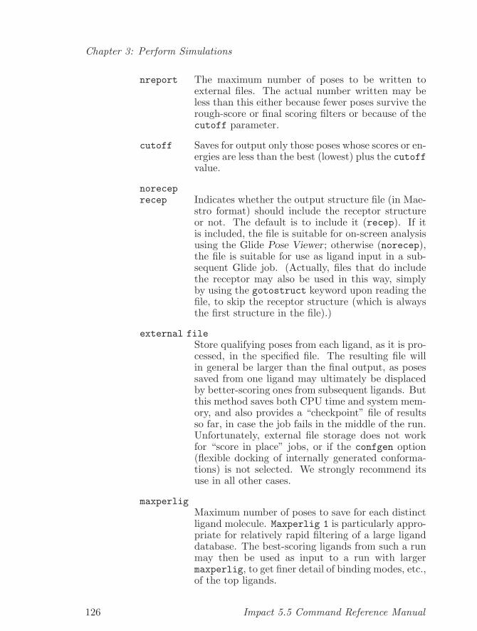
Chapter 3: Perform Simulations
nreport The maximum number of poses to be written toexternal files. The actual number written may beless than this either because fewer poses survive therough-score or final scoring filters or because of thecutoff parameter.
cutoff Saves for output only those poses whose scores or en-ergies are less than the best (lowest) plus the cutoffvalue.
noreceprecep Indicates whether the output structure file (in Mae-
stro format) should include the receptor structureor not. The default is to include it (recep). If itis included, the file is suitable for on-screen analysisusing the Glide Pose Viewer; otherwise (norecep),the file is suitable for use as ligand input in a sub-sequent Glide job. (Actually, files that do includethe receptor may also be used in this way, simplyby using the gotostruct keyword upon reading thefile, to skip the receptor structure (which is alwaysthe first structure in the file).)
external fileStore qualifying poses from each ligand, as it is pro-cessed, in the specified file. The resulting file willin general be larger than the final output, as posessaved from one ligand may ultimately be displacedby better-scoring ones from subsequent ligands. Butthis method saves both CPU time and system mem-ory, and also provides a “checkpoint” file of resultsso far, in case the job fails in the middle of the run.Unfortunately, external file storage does not workfor “score in place” jobs, or if the confgen option(flexible docking of internally generated conforma-tions) is not selected. We strongly recommend itsuse in all other cases.
maxperligMaximum number of poses to save for each distinctligand molecule. Maxperlig 1 is particularly appro-priate for relatively rapid filtering of a large liganddatabase. The best-scoring ligands from such a runmay then be used as input to a run with largermaxperlig, to get finer detail of binding modes, etc.,of the top ligands.
126 Impact 5.5 Command Reference Manual
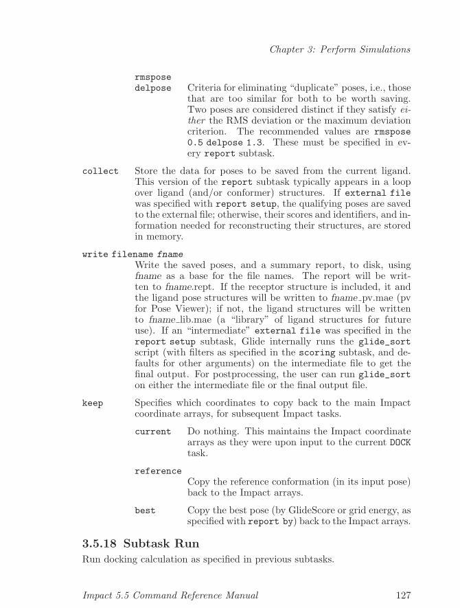
Chapter 3: Perform Simulations
rmsposedelpose Criteria for eliminating “duplicate” poses, i.e., those
that are too similar for both to be worth saving.Two poses are considered distinct if they satisfy ei-ther the RMS deviation or the maximum deviationcriterion. The recommended values are rmspose0.5 delpose 1.3. These must be specified in ev-ery report subtask.
collect Store the data for poses to be saved from the current ligand.This version of the report subtask typically appears in a loopover ligand (and/or conformer) structures. If external filewas specified with report setup, the qualifying poses are savedto the external file; otherwise, their scores and identifiers, and in-formation needed for reconstructing their structures, are storedin memory.
write filename fnameWrite the saved poses, and a summary report, to disk, usingfname as a base for the file names. The report will be writ-ten to fname.rept. If the receptor structure is included, it andthe ligand pose structures will be written to fname pv.mae (pvfor Pose Viewer); if not, the ligand structures will be writtento fname lib.mae (a “library” of ligand structures for futureuse). If an “intermediate” external file was specified in thereport setup subtask, Glide internally runs the glide_sortscript (with filters as specified in the scoring subtask, and de-faults for other arguments) on the intermediate file to get thefinal output. For postprocessing, the user can run glide_sorton either the intermediate file or the final output file.
keep Specifies which coordinates to copy back to the main Impactcoordinate arrays, for subsequent Impact tasks.
current Do nothing. This maintains the Impact coordinatearrays as they were upon input to the current DOCKtask.
referenceCopy the reference conformation (in its input pose)back to the Impact arrays.
best Copy the best pose (by GlideScore or grid energy, asspecified with report by) back to the Impact arrays.
3.5.18 Subtask Run
Run docking calculation as specified in previous subtasks.
Impact 5.5 Command Reference Manual 127
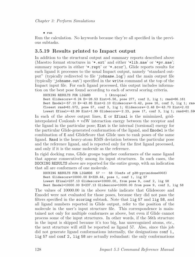
Chapter 3: Perform Simulations
• run
Run the calculation. No keywords because they’re all specified in the previ-ous subtasks.
3.5.19 Results printed to Impact output
In addition to the structural output and summary reports described above(Maestro format structures in ‘*.ext’ and either ‘*lib.mae’ or ‘*pv.mae’;summary reports in either ‘*.rept’ or ‘*.scor’), Glide reports results foreach ligand it processes to the usual Impact output, namely “standard out-put” (typically redirected to file ‘jobname.log’) and the main output file(typically ‘jobname.out’) specified in the write command at the top of theImpact input file. For each ligand processed, this output includes informa-tion on the best pose found according to each of several scoring criteria.
DOCKING RESULTS FOR LIGAND 1 (Atropine)
Best Glidescore=-6.24 E=-26.53 Eint=5.56, pose 277, conf 2, lig 1; rmsd=66.161
Best Emodel=-57.10 E=-43.85 Eint=2.10 Glidescore=-5.42, pose 16, conf 3, lig 1; rmsd=61.597
Closest rmsd=61.572, pose 57, conf 3, lig 1; Glidescore=-2.48 E=-43.70 Eint=2.02
Lowest Efinal=-43.99 Eint=1.99 Glidescore=-2.23, pose 17, conf 3, lig 1; rmsd=61.596
In each of the above output lines, E or Efinal is the minimized, grid-interpolated Coulomb + vdW interaction energy between the receptor andthe ligand in the particular pose; Eint is the internal (torsional) energy forthe particular Glide-generated conformation of the ligand, and Emodel is thecombination of E and GlideScore that Glide uses to rank poses of the sameligand. Rmsd is the heavy-atom RMS deviation between the particular poseand the reference ligand, and is reported only for the first ligand processed,and only if it is the same molecule as the reference.In rigid docking runs, Glide groups together conformers of the same ligandthat appear consecutively among its input structures. In such cases, theDOCKING RESULTS above are reported for the entire group, with an indicationthat all are conformers of one molecule.
DOCKING RESULTS FOR LIGANDS 57 -- 58 (Confs of p38-pyrimidone0003)
Best Glidescore=10000.00 E=329.44, pose 1, conf 1, lig 57
Lowest Efinal=237.13 Glidescore=10000.00, from pose 9, conf 2, lig 58
Best Emodel=10000.00 E=237.13 Glidescore=10000.00 from pose 9, conf 2, lig 58
The values of 10000.00 in the above table indicate that Glidescore andEmodel were not evaluated for those poses, because they did not pass thefilters specified in the scoring subtask. Note that lig 57 and lig 58, andall ligand numbers reported in Glide output, refer to the position of themolecule in the user’s input structure file. This correspondence is main-tained not only for multiple conformers as above, but even if Glide cannotprocess some of the input structures. In other words, if the 56th structurein the input is skipped because it’s too big, has unrecognized atoms, etc.,the next structure will still be reported as ligand 57. Also, since this jobdid not generate ligand conformations internally, the designations conf 1,lig 57 and conf 2, lig 58 are actually redundant: the only conformations
128 Impact 5.5 Command Reference Manual
Chapter 3: Perform Simulations
analyzed are those that were in the input, so lig 57 is the first conformationof this molecule, and lig 58 is the second.In addition to the above output of “best” poses, Glide will print tables ofposes processed from each ligand, after the rough-score and energy mini-mization steps, if the verbosity parameter is set higher than 1. Since thisoutput can run to tens or hundreds of poses per ligand, we strongly recom-mend against setting verbosity that high in jobs with many ligands, exceptfor testing or debugging purposes.
Impact 5.5 Command Reference Manual 129

Chapter 3: Perform Simulations
130 Impact 5.5 Command Reference Manual
Chapter 4: Advanced Input Scripts
4 Advanced Input Scripts
In this chapter, we will discuss some advanced features of Impact inputscripts (DICE scripts). You will find it is very powerful after you spend sometime with it. You can manipulate internal data lists; you can use if elseendif statements inside the input file; you can specify a while endwhile doloop to control a simulation; you can even call a previously written scriptsubroutine to perform a common task, etc.
4.1 BackgroundAs you have probably noticed already, at its core Impact is a program forprocessing a series of commands in a control file, the input file. These basiccommands comprise a set of powerful tools for modeling complex chemi-cal structures; the three levels of commands are the task, subtask and the“program” levels. The last level is independent of which task or subtaskis presently being used, and consists of a set of data structures and pro-gramming constructs. At the program level it is possible to write programsdefining the execution of Impact, as well as to access and modify internalImpact data structures using lists. For example, counters can be createdand incremented, tasks and subtasks can be executed inside of looping con-structs, and the internal state of Impact can be examined or modified.The task level communicates to the program that a group of complex op-erations will be performed. Each task is invoked by giving the task namealone on a line of the input file. For example, for the dynamics task, whichintegrates the equations of motion for a chemical system, the word dynamicsappears alone on a line. This causes the program to branch into the portionthat performs a molecular dynamics simulation. The word quit (alone on aline) ends the current task and returns the execution pathway to the maincontroller. At this point the subsequent task is performed.Inside each task a series of subtasks are performed. Here details are givenabout the particular pathways to follow or parameters to use in the con-text of the current task. For example, in the task setmodel (which specifiesthe features of the energy model to be used in simulations) the subtasksetpotential specifies the types and weights to be used in the energy func-tion. The subtask mixture takes a solute molecule and places it in a box ofsolvent molecules.At the lowest level, programming constructs and data structures are ma-nipulated in a task/subtask independent way. When these programmingconstructs are used, the commands appear by themselves on a commandline. For example, in using Impact’s conditional construct, an if block, aline such as ‘if ’a’ eq ’b’ dynamics endif’ would not work, however, thefollowing multiple line command is acceptable:
if ’a’ eq ’b’
dynamics ! do the task dynamics if ’a’ and ’b’ are equal
Impact 5.5 Command Reference Manual 131
Chapter 4: Advanced Input Scripts
< some dynamics operations >
quit
endif
The existence of a programming language inside of Impact greatly increasesboth its ease of use and the ability to express complex computational exper-iments that might otherwise be all but impossible to perform.The data structures available in Impact are scalars and lists, which corre-spond to variables and constants in typical programming languages. Listsare perhaps most similar to arrays of records, and may contain one number,or thousands. An Impact list is like a two dimensional array in containingrows and columns; the number of rows is called the size and the number ofcolumns is called the dimension of the list. An element of a list is, for exam-ple, the value at row 1 and column 1.1 Generally the size of a list is flexibleand will grow as needed, whereas the dimension is fixed and is determinedby how the list was first created. Arithmetic operations on lists normallyrequire that both operands be of the same dimension or that one be scalar.When used as a logical expression, an empty list will be the same as a falseexpression. Conversely, a list with any elements in it is a true expression.Theelements of lists can be referenced in a number of ways.
4.1.1 Lists
For the user of Impact, the primary means to manipulate data is using thedata structures referred to here as lists or tables.2 The names of lists arealways placed within single quotes when used, and these names have max-imum lengths of 30 characters. All characters supported by the computerare allowed with the exceptions of single quotes and underscores. Some validnames are ’Validname’, ’themotherofalllists’’ and ’abc123me&u’. Note thatunderscores should not be used in list names since they are used to delimitcolumns of real numbers.A list is a collection of related elements with a well defined structure, both insize and dimension. Some major types of list structures in Impact are atom,residue, molecule and species number; these types of structure are automat-ically recognized within Impact. Properties such as charge and surface areaare frequently calculated in one of these types of list. Other types of listmay also be used, for example lists to store properties with cartesian (x, y,z) components, or lists of position, force and velocity. Another type of listis a set of of statistics containing the three components sum, average andstandard deviation.There are two broad catagories of lists, user defined and internal. Mostproperties are shared by these two types. However, several internal lists
1 A list with size 1 and dimension 1 would be the same as a scalar variable found in manycomputer languages.
2 Lists and tables are equivalent.
132 Impact 5.5 Command Reference Manual
Chapter 4: Advanced Input Scripts
are tied to the internal system state. Internal lists are “peep holes” intothe major Impact data structures. These lists are created the first timethey are referenced as a copy of the current state of the related Impactdata structure.3 These lists are are structured according to the informationcontained within them, since Impact is able to create the structure of thelist from the information in the chemical system currently being used. Forexample, the list surfacearea is structured by atom.Both internal (built-in) and user defined lists only “come into existence”the first time they are specified. Because internal lists are only copies ofthe internal data structures used by Impact, they stay fixed after the initialcopy is made, even if subsequent Impact tasks modify the correspondinginternal data structures. These lists are only “refreshed” with current datawhen used the first time. To subsequently update the lists with new datathe old copies are first erased using the reset command, after which anysubsequent use of the list will cause it to be updated with the current Impactdata. For later updating, the reset command must be used again. Manyof these built-in lists are useful for storing information from tasks for laterretrieval. This is particularly useful if dynamics is being run on the samesystem many times. Then the average of the averages of individual runs canbe obtained.While internal lists may be used before being assigned values, they will some-times be undefined until certain subtasks are executed. For example, thebondlist has a component that is the actual bond energy, but this assumesthat the parameters have been defined by using the setmodel task. Thelist Current.kinetic contains the current kinetic energy but this requiresthat dynamics has been run. Other internal lists requiring that a task orsubtask be performed before they may be used are the lists for surface area(surfacearea) and the rms deviation (rms.dev.atom), where the analysistask must be run and the appropriate subtasks performed before the lists areproperly defined. The creation of these lists is done automatically, and theymay be used after the subtasks are run. The cartesian coordinate list (cord)can be used at any point after the task create is performed. In general,the contents of the list will vary depending on when the list is used. Forexample, the values of cord change after a dynamics run. Remember thecaveat that the value of internal lists are set as soon as they are used, butif the values need to be updated the command reset must be used to clearthe old contents of the list. The next use of the list name will then causethe values of the list to be updated.
4.1.2 Internal Lists
The following tables show the internal (“built-in”) lists that carry the currentstate of various Impact internal data structures.
3 We emphasize that internal lists are user-accessible copies of the Impact data structures.
Impact 5.5 Command Reference Manual 133
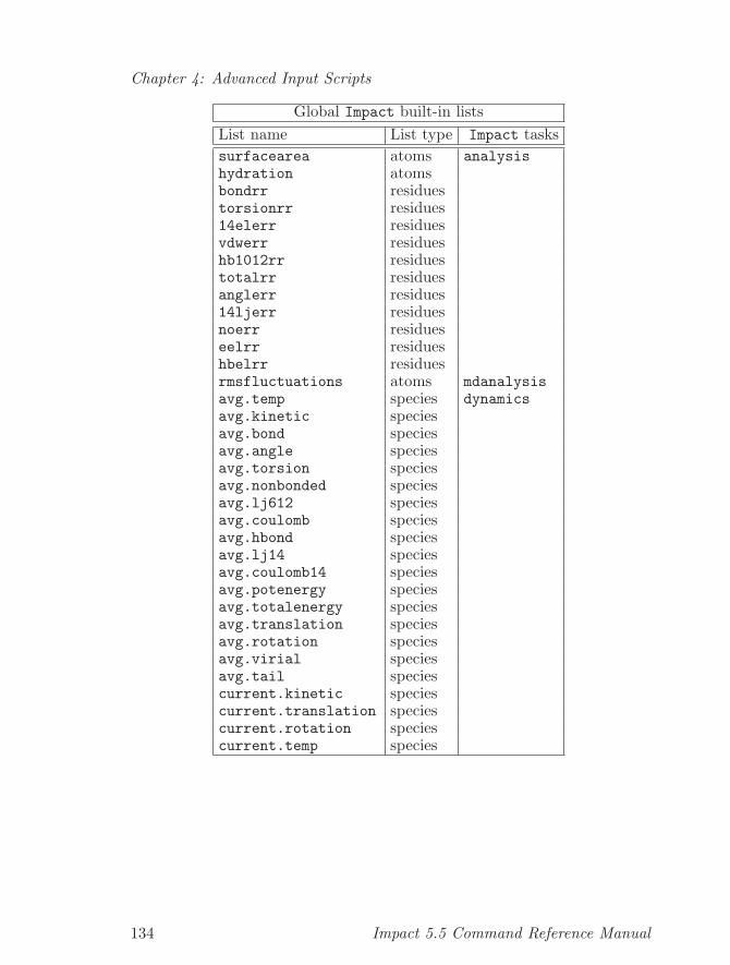
Chapter 4: Advanced Input Scripts
Global Impact built-in listsList name List type Impact taskssurfacearea atoms analysishydration atomsbondrr residuestorsionrr residues14elerr residuesvdwerr residueshb1012rr residuestotalrr residuesanglerr residues14ljerr residuesnoerr residueseelrr residueshbelrr residuesrmsfluctuations atoms mdanalysisavg.temp species dynamicsavg.kinetic speciesavg.bond speciesavg.angle speciesavg.torsion speciesavg.nonbonded speciesavg.lj612 speciesavg.coulomb speciesavg.hbond speciesavg.lj14 speciesavg.coulomb14 speciesavg.potenergy speciesavg.totalenergy speciesavg.translation speciesavg.rotation speciesavg.virial speciesavg.tail speciescurrent.kinetic speciescurrent.translation speciescurrent.rotation speciescurrent.temp species
134 Impact 5.5 Command Reference Manual
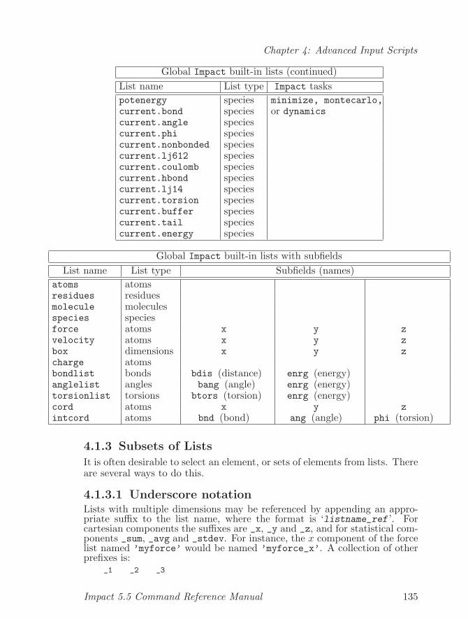
Chapter 4: Advanced Input Scripts
Global Impact built-in lists (continued)List name List type Impact taskspotenergy species minimize, montecarlo,current.bond species or dynamicscurrent.angle speciescurrent.phi speciescurrent.nonbonded speciescurrent.lj612 speciescurrent.coulomb speciescurrent.hbond speciescurrent.lj14 speciescurrent.torsion speciescurrent.buffer speciescurrent.tail speciescurrent.energy species
Global Impact built-in lists with subfieldsList name List type Subfields (names)
atoms atomsresidues residuesmolecule moleculesspecies speciesforce atoms x y zvelocity atoms x y zbox dimensions x y zcharge atomsbondlist bonds bdis (distance) enrg (energy)anglelist angles bang (angle) enrg (energy)torsionlist torsions btors (torsion) enrg (energy)cord atoms x y zintcord atoms bnd (bond) ang (angle) phi (torsion)
4.1.3 Subsets of Lists
It is often desirable to select an element, or sets of elements from lists. Thereare several ways to do this.
4.1.3.1 Underscore notationLists with multiple dimensions may be referenced by appending an appro-priate suffix to the list name, where the format is ‘listname_ref ’. Forcartesian components the suffixes are _x, _y and _z, and for statistical com-ponents _sum, _avg and _stdev. For instance, the x component of the forcelist named ’myforce’ would be named ’myforce_x’. A collection of otherprefixes is:
_1 _2 _3
Impact 5.5 Command Reference Manual 135
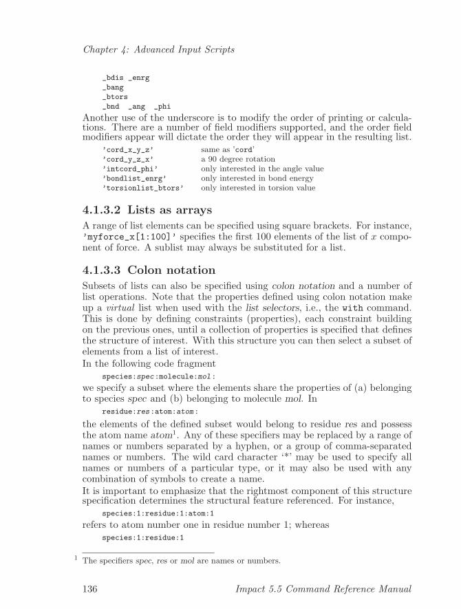
Chapter 4: Advanced Input Scripts
_bdis _enrg
_bang
_btors
_bnd _ang _phi
Another use of the underscore is to modify the order of printing or calcula-tions. There are a number of field modifiers supported, and the order fieldmodifiers appear will dictate the order they will appear in the resulting list.
’cord_x_y_z’ same as ’cord’’cord_y_z_x’ a 90 degree rotation’intcord_phi’ only interested in the angle value’bondlist_enrg’ only interested in bond energy’torsionlist_btors’ only interested in torsion value
4.1.3.2 Lists as arrays
A range of list elements can be specified using square brackets. For instance,’myforce_x[1:100]’ specifies the first 100 elements of the list of x compo-nent of force. A sublist may always be substituted for a list.
4.1.3.3 Colon notation
Subsets of lists can also be specified using colon notation and a number oflist operations. Note that the properties defined using colon notation makeup a virtual list when used with the list selectors, i.e., the with command.This is done by defining constraints (properties), each constraint buildingon the previous ones, until a collection of properties is specified that definesthe structure of interest. With this structure you can then select a subset ofelements from a list of interest.In the following code fragment
species:spec:molecule:mol:
we specify a subset where the elements share the properties of (a) belongingto species spec and (b) belonging to molecule mol. In
residue:res:atom:atom:
the elements of the defined subset would belong to residue res and possessthe atom name atom1. Any of these specifiers may be replaced by a range ofnames or numbers separated by a hyphen, or a group of comma-separatednames or numbers. The wild card character ‘*’ may be used to specify allnames or numbers of a particular type, or it may also be used with anycombination of symbols to create a name.It is important to emphasize that the rightmost component of this structurespecification determines the structural feature referenced. For instance,
species:1:residue:1:atom:1
refers to atom number one in residue number 1; whereasspecies:1:residue:1
1 The specifiers spec, res or mol are names or numbers.
136 Impact 5.5 Command Reference Manual
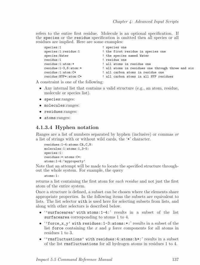
Chapter 4: Advanced Input Scripts
refers to the entire first residue. Molecule is an optional specification. Ifthe species or the residue specification is omitted then all species or allresidues are implied. Here are some examples:
species:1 ! species one
species:1:residue:1 ! the first residue in species one
species:Water ! the species named Water
residue:1 ! residue one
residue:1:atom:* ! all atoms in residue one
residue:1-3,6:atom:* ! all atoms in residues one through three and six
residue:1:atom:C* ! all carbon atoms in residue one
residue:HYP*:atom:C* ! all carbon atoms in all HYP residues
A constraint is one of the following:• Any internal list that contains a valid structure (e.g., an atom, residue,
molecule or species list).• species:ranges:• molecules:ranges:• residues:ranges:• atoms:ranges:
4.1.3.4 Hyphen notation
Ranges are a list of numbers separated by hyphen (inclusive) or commas ora list of strings with or without wild cards, the ‘*’ character.
residues:1-4:atoms:CA,C,N:
molecules:1:atoms:1,3-5:
species:1:
residues:*:atoms:C*:
atoms:1-4:’myproperty’
Note that an attempt will be made to locate the specified structure through-out the whole system. For example, the query
atoms:1:
returns a list containing the first atom for each residue and not just the firstatom of the entire system.Once a structure is defined, a subset can be chosen where the elements shareappropriate properties. In the following items the subsets are equivalent tolists. The list selector with is used here for selecting subsets from lists, andalong with other selectors is described below.• ‘’surfacearea’ with atoms:1-4:’ results in a subset of the list
surfacearea corresponding to atoms 1 to 4.• ‘’force_x_y’ with residues:1-3:atoms:*:’ results in a subset of the
list force containing the x and y force components for all atoms inresidues 1 to 3.
• ‘’rmsfluctuations’ with residues:4:atoms:h*:’ results in a subsetof the list rmsfluctuations for all hydrogen atoms in residues 1 to 4.
Impact 5.5 Command Reference Manual 137
Chapter 4: Advanced Input Scripts
Having selected the range of properties you wish to work with you can dooperations on those properties. A large library of arithmetic and statisticalfunctions is available.
4.1.4 List Creation
Lists are generally created using the command put; however, create hassome uses that the other doesn’t.
4.1.4.1 PutThe put statement is used to assign values to lists. In doing so the list iscreated if it didn’t already exist.
put ’expression’ into ’list’
4.1.4.2 Create
Create a new list.
4.1.5 List Selection
As noted above, the properties describing subsets of lists are built up us-ing several notations, and subsets of lists are actually constructed using listconstructors like with; this and other list functions are described here. Theresultant subsets are often placed in new lists, which is the convention fol-lowed in these examples.
4.1.5.1 WithThe function with returns those elements in one list that are found in bothlists. Atoms, molecules, residues, and species are recognized by these func-tions. In the following example those elements in the ’charge’ list belongingto atoms with names beginning with the letters ’CA’ are selected.
put ’charge’ with atoms:CA*: into ’result’
4.1.5.2 WithonlyThe withonly function extracts those elements in the list whose atom,molecule, residue or species specification match the entire target specifi-cation. In the following example, only those bonds containing both CA*and N* atoms are extracted. In contrast the selector with returns all bondswith CA or N atoms.
put ’bondlist’ withonly atoms:CA*,N*: into ’result’
4.1.5.3 WithoutThe without function returns those elements in the first list that do nothave relations with the second list. This example extracts those elementsfrom the torsional internal coordinate list that are not hydrogen atoms.
put ’intcord_phi’ without atoms:h*: into ’result’
138 Impact 5.5 Command Reference Manual
Chapter 4: Advanced Input Scripts
4.1.5.4 ByThe by function returns a list that is the result of applying the previousfunction over a long list split up by its structures. By requires two lists.One of these is called the limit and must be of type residue, molecule orspecies, and the other is called the range and must be of type atom, residueor molecule. The result is a list the same length as the limit, with eachelement storing the result of applying the previous function over the rangesplit up along the structures of the limit. The functions you can apply byto include: abs, int, avg, stat, sum, sum2, ln, sin, cos, tab, asin, acos,and atan. The following example results in a list of type residue with eachelement storing the sum of the atom charges for each residue. (In most casesthis would be a of list of zeros, ones and minus ones.)
put sum ’charge’ by ’residue’ into ’result’
4.2 Operations on DataA range of functions and list-selectors are available, including the standardarithmetic expressions and a set of functions defined solely for lists. A listexpression is a list or any arithmetic or functional expression that resultsin a list, and a list-expression may always be substituted for a list. Thearithmetic operators include exponentiation (^), multiplication (*), division(/), addition (+), subtraction (binary -) and negation (unary -). These maybe applied to constants, such as ‘2 * 2’, or used as list operators. Operationsmay be performed between lists with common structures, or between listsand scalars.When operations occur between lists of different dimensions, the result of theoperation inherits the dimensionality of the list of higher dimension. Con-sider the following examples in which ’myforces’ is a list of atomic forceshaving an atomic cartesian (x, y, z) structure, ’jscal’ is a user-defined listhaving a simple atomic structure, and ’const’ is a scalar sonstant.
’myforces_x’ * ’jscal’
multiplies the corresponding elements of the x component of ’myforces’ and’jscal’.
4.2.1 General Operations
Arithmetic functions are applied to a list in one of three ways:1. If one of the operators is a single element, the operation is done with
the value of that element against all the values in the other list. (Thatmeans that you can multiply an entire list by a single constant.)
2. Some functions take only a single list and return a few elements ofinformation about that list, such as the average value of the list, or itsfour (4) greatest values.
3. If you are applying a function between two lists and both lists have sizegreater than 1, that function will be applied to each element in the two
Impact 5.5 Command Reference Manual 139
Chapter 4: Advanced Input Scripts
lists that correspond to each other. This means you can add the valuesof two lists in an element by element manner.1 + ’mydata’ ! every element gains 1
’mydata’ + ’mydata’ ! <--- these are
2 * ’mydata’ ! the same
’mydata’ pow 0.33333 ! cube root
7 lowest ’mydata’ ! sorted lowest 7 elements
avg ’mydata’ ! the list average put in a new 1 element list
(sum ’mydata’)/(length ’mydata’) ! silly way to avg
(’newdata’+’olddata’)/2 ! result is a new list consisting of the
! average values of each of the list elements
’myforces_x’ * ’const’
multiplies all the x components of ’myforces’ by the value of ’const’.The command
’myforces’ + 2.0
adds the value of 2.0 to all of the components (x, y, z) of ’myforces’.
140 Impact 5.5 Command Reference Manual
Chapter 4: Advanced Input Scripts
General OperatorsOperator Function Parameters Units+ Addition 2- Subtraction 2* Multiplication 2/ Division 2abs Absolute value 1acos Arc Cosine 1 radianadd Addition 2asin Arc Sine 1 radianatan Arc Tangent 1 radianavg Average 1avgb Special case of by function 2by Apply a 1 parameter function over
a list of values(e.g. sum ’charge’ by ’residues’)
cos Cosine 1 radiandistance Distance Function 2 cord unitsdiv Division 2grdist Greatest Distance 2 atoms unitsgreatest N Maximum values 2
e.g., 3 greatest ’bondlist bdis’index Extracts an element from a list 2
e.g. index 10 ’charge’gets the 10th value from the charge list)
int Truncation 1length Size of list 1lowest N Minimum values 2ln Natural Log 1^ Exponentiation 2exp Exponentiation (base e) 1lstdist Least Distance 2 atoms unitsalldist All distances 2 atoms unitshist Histogram 2max Maximum value 1min Minumum value 1mul Multiplication 2pow Power function (base 10) 1rand Random number 1runavg Running Average 1
Impact 5.5 Command Reference Manual 141
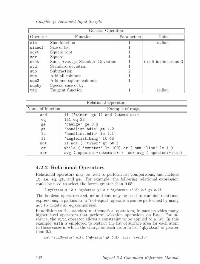
Chapter 4: Advanced Input Scripts
General OperatorsOperator Function Parameters Unitssin Sine function 1 radiansizeof Size of list 1sqrt Square root 1sqr Square 1stat Sum, Average, Standard Deviation 1 result is dimension 3std Standard deviation 1sub Subtraction 2sum Add all columns 1sum2 Add and square columns 1sumby Special case of bytan Tangent function 1 radian
Relational OperatorsName of function Example of usage
and if (’timer’ gt 1) and (atoms:ca:)eq 131 eq 23ge ’charge’ ge 0.2gt ’bondlist bdis’ gt 1.2le ’bondlist bdis’ le 1.1lt ’anglelist bang’ lt 45not if not ( ’timer’ gt 50 )or while ( ’counter’ lt 100) or ( sum ’list’ lt 1 )xor avg ( species:*:atoms:c*:) xor avg ( species:*:ca:)
4.2.2 Relational Operators
Relational operators may be used to perform list comparisons, and includelt, le, eq, gt, and ge. For example, the following relational expressioncould be used to select the forces greater than 0.05:
(’myforces_x’^2 + ’myforces_y’^2 + ’myforces_z’^2)^0.5 gt 0.05
The boolean operators and, or and not may be used to combine relationalexpressions; in particular, a “not-equal” operation can be performed by usingnot to negate an eq comparison.In addition to the standard mathematical operators, Impact provides manyhigher level operators that perform selection operations on lists. For in-stance, the with operator allows a constraint to be applied to a list. In thisexample, with is employed to restrict the list of surface area for each atomto those cases in which the charge on each atom in list ’qbyatom’ is greaterthan 0.2:
put ’surfbyatom’ with (’qbyatom’ gt 0.2) into ’result’
142 Impact 5.5 Command Reference Manual
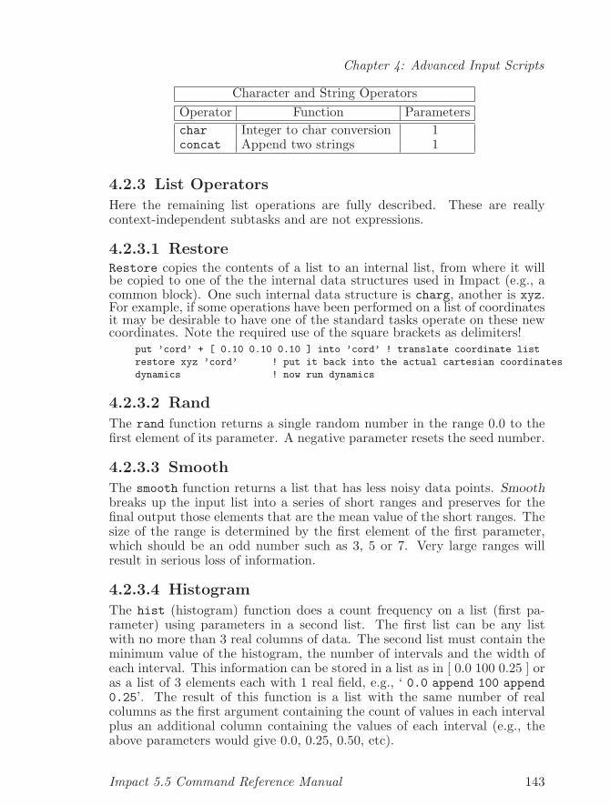
Chapter 4: Advanced Input Scripts
Character and String OperatorsOperator Function Parameterschar Integer to char conversion 1concat Append two strings 1
4.2.3 List Operators
Here the remaining list operations are fully described. These are reallycontext-independent subtasks and are not expressions.
4.2.3.1 RestoreRestore copies the contents of a list to an internal list, from where it willbe copied to one of the the internal data structures used in Impact (e.g., acommon block). One such internal data structure is charg, another is xyz.For example, if some operations have been performed on a list of coordinatesit may be desirable to have one of the standard tasks operate on these newcoordinates. Note the required use of the square brackets as delimiters!
put ’cord’ + [ 0.10 0.10 0.10 ] into ’cord’ ! translate coordinate list
restore xyz ’cord’ ! put it back into the actual cartesian coordinates
dynamics ! now run dynamics
4.2.3.2 Rand
The rand function returns a single random number in the range 0.0 to thefirst element of its parameter. A negative parameter resets the seed number.
4.2.3.3 Smooth
The smooth function returns a list that has less noisy data points. Smoothbreaks up the input list into a series of short ranges and preserves for thefinal output those elements that are the mean value of the short ranges. Thesize of the range is determined by the first element of the first parameter,which should be an odd number such as 3, 5 or 7. Very large ranges willresult in serious loss of information.
4.2.3.4 Histogram
The hist (histogram) function does a count frequency on a list (first pa-rameter) using parameters in a second list. The first list can be any listwith no more than 3 real columns of data. The second list must contain theminimum value of the histogram, the number of intervals and the width ofeach interval. This information can be stored in a list as in [ 0.0 100 0.25 ] oras a list of 3 elements each with 1 real field, e.g., ‘ 0.0 append 100 append0.25’. The result of this function is a list with the same number of realcolumns as the first argument containing the count of values in each intervalplus an additional column containing the values of each interval (e.g., theabove parameters would give 0.0, 0.25, 0.50, etc).
Impact 5.5 Command Reference Manual 143
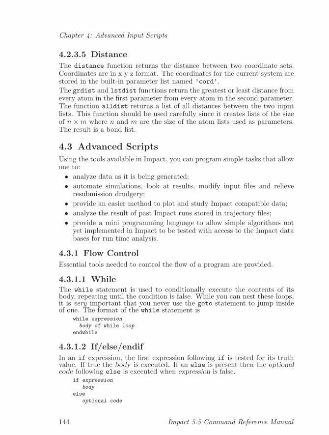
Chapter 4: Advanced Input Scripts
4.2.3.5 Distance
The distance function returns the distance between two coordinate sets.Coordinates are in x y z format. The coordinates for the current system arestored in the built-in parameter list named ’cord’.The grdist and lstdist functions return the greatest or least distance fromevery atom in the first parameter from every atom in the second parameter.The function alldist returns a list of all distances between the two inputlists. This function should be used carefully since it creates lists of the sizeof n ×m where n and m are the size of the atom lists used as parameters.The result is a bond list.
4.3 Advanced ScriptsUsing the tools available in Impact, you can program simple tasks that allowone to:• analyze data as it is being generated;• automate simulations, look at results, modify input files and relieve
resubmission drudgery;• provide an easier method to plot and study Impact compatible data;• analyze the result of past Impact runs stored in trajectory files;• provide a mini programming language to allow simple algorithms not
yet implemented in Impact to be tested with access to the Impact databases for run time analysis.
4.3.1 Flow Control
Essential tools needed to control the flow of a program are provided.
4.3.1.1 WhileThe while statement is used to conditionally execute the contents of itsbody, repeating until the condition is false. While you can nest these loops,it is very important that you never use the goto statement to jump insideof one. The format of the while statement is
while expression
body of while loop
endwhile
4.3.1.2 If/else/endifIn an if expression, the first expression following if is tested for its truthvalue. If true the body is executed. If an else is present then the optionalcode following else is executed when expression is false.
if expression
body
else
optional code
144 Impact 5.5 Command Reference Manual
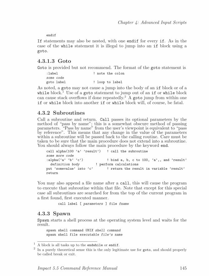
Chapter 4: Advanced Input Scripts
endif
If statements may also be nested, with one endif for every if. As in thecase of the while statement it is illegal to jump into an if block using agoto.
4.3.1.3 GotoGoto is provided but not recommend. The format of the goto statement is
:label ! note the colon
some code
goto label ! loop to label
As noted, a goto may not cause a jump into the body of an if block or of awhile block.1 Use of a goto statement to jump out of an if or while blockcan cause stack overflows if done repeatedly.2 A goto jump from within oneif or while block into another if or while block will, of course, be fatal.
4.3.2 SubroutinesCall a subroutine and return. Call passes its optional parameters by themethod of “pass by name”; this is a somewhat obscure method of passingparameters. “Pass by name” from the user’s viewpoint is equivalent to “passby reference”. This means that any change in the value of the parameterswithin a subroutine will be passed back to the calling routine. Care must betaken to be sure that the main procedure does not extend into a subroutine.You should always follow the main procedure by the keyword end.
call alpha(100 ’a’ ’result’) ! call the subroutine
some more code
:alpha(’a’ ’b’ ’c’) ! bind a, b, c to 100, ’a’,, and ’result’
definition body ! perform calculations
put ’somevalue’ into ’c’ ! return the result in variable ’result’
return
You may also append a file name after a call, this will cause the programto execute that subroutine within that file. Note that except for this specialcase all subroutines are searched for from the top of the current program ina first found, first executed manner.
call label [ parameters ] file fname
4.3.3 SpawnSpawn starts a shell process at the operating system level and waits for theresult.
spawn shell command UNIX shell command
spawn shell file executable file’s name
1 A block is all tasks up to the endwhile or endif.2 In a purely theoretical sense this is the only legitimate use for goto, and should properly
be called break or exit.
Impact 5.5 Command Reference Manual 145
Chapter 4: Advanced Input Scripts
4.3.4 Lists as Parameters
Numeric lists can be placed anywhere a number normally can be specified;if an operation requires a scalar value then the first element from the list’snumeric field is used. Short character lists can also be used to hold filenames,which is especially useful when many files are being created and uniquenames are needed. Though we are getting ahead of ourselves by discussingspecific tasks in the following example,3 it does illustrate the use of differentlist operations and types of lists. Here we loop over the run subtask indynamics4. While it would often only be desired to save the final state ina restart file, saving intermediate states assures that intermediate work hasbeen saved if the job is terminated for any reason. A series of trajectory filesmight be saved in the same way.
’i’ is a list that is used as if it were an integer variable.
’filename’is a list of characters that is modified in each stage of the dy-namics run. Thus, unique trajectory files may be written foreach phase.
$protein$ and $ps$are string constants. Note the use of the dollar sign to delimitstring constants.
3 The example uses meta-variables that are explained in Chapter 2 [Setup System], page 15.4 The task dynamics is described in Section 3.2 [Dynamics], page 60
146 Impact 5.5 Command Reference Manual
Chapter 5: Trouble Shooting
5 Trouble Shooting
This chapter describes some common problems with starting or runningImpact. Naturally, we hope that you will never need to use this chapter.However, if you have problems using Impact, you may find useful advicehere. You may also contact us using the information on the cover page.
5.1 Problems Getting StartedThis section describes how to overcome some problems in starting up yourImpact jobs. The next section describes problems that occur during jobexecution.
5.1.1 Environment variable SCHRODINGER not set.
Before running Impact, or any Schrodinger product, on any particularmachine, you must set the environment variable SCHRODINGER to yourSchrodinger installation directory. If this environment variable is not setcorrectly, you will be told directly:
unix% /usr/apps/schrodinger/impact -i dynamics_job.inp
ERROR: SCHRODINGER is undefined
unix%
Or if the program stops at automatic atom-typing for ligand molecules, itwill prints out message like this:
%IMPACT-I (readhead): input file 23 has no header information.
%IMPACT-I (readhead): input file 23 has no header information.
PARM read from file paramstd.dat
Environment variables MMSHARE_EXEC and OPLS_DIR not defined
Set OPLS_DIR so that ATOMTYPE can find data files
It is easy to fix this problem, first check whether SCHRODINGER is set or not,enter the command
% echo $SCHRODINGER
If you see this environment variable is not set or set to a wrong directory,change it to a right directory. If you are running C shell (csh) or tcsh, typethe command
% setenv SCHRODINGER your Schrodinger installation directory
or if you are using bash, sh or ksh, type the command% export SCHRODINGER=your Schrodinger installation directory
5.1.2 Bad residue labelThe current Impact program requires the user to separate a ligand moleculefrom the protein in the input PDB files. This means PDB files for proteinsmust contain only the regular amino acids and buried waters, but not anonstandard residue name unless it has previously been defined. Here is anexample of a PDB file containing a residue named NOA (NAPHTHYLOXY-ACETYL):
Impact 5.5 Command Reference Manual 147
Chapter 5: Trouble Shooting
...............
...............
ATOM 1485 CD2 NOA I 201 4.098 9.733 20.948 0.50 20.67
ATOM 1486 CD1 NOA I 201 6.413 10.411 21.013 0.50 20.84
ATOM 1487 CE1 NOA I 201 6.706 9.320 21.850 0.50 21.17
ATOM 1488 CZ1 NOA I 201 5.694 8.437 22.228 0.50 20.95
ATOM 1489 CE2 NOA I 201 4.385 8.645 21.778 0.50 21.01
ATOM 1490 CZ3 NOA I 201 1.771 9.028 20.869 0.50 21.10
ATOM 1491 CE3 NOA I 201 2.786 9.926 20.504 0.50 20.98
ATOM 1492 CZ2 NOA I 201 3.379 7.740 22.165 0.50 21.13
ATOM 1493 CH2 NOA I 201 2.067 7.934 21.703 0.50 21.20
ATOM 1494 C NOA I 201 4.312 13.086 17.860 0.50 18.24
ATOM 1493 CH2 NOA I 201 2.067 7.934 21.703 0.50 21.20
ATOM 1494 C NOA I 201 4.312 13.086 17.860 0.50 18.24
ATOM 1495 O NOA I 201 5.155 13.679 17.160 0.50 17.86
..............
..............
The program will stop because (we presume) there is no template file forresidue NOA. The message printed out in the primary output file looks likethis:
*** BAD RESIDUE LABEL NOA
%IMPACT-E (die): Fatal error at line 5
At present, the user has to separate the NOA molecule from the proteinresidues in the PDB file, and read it in through type ligand:
build primary name hiv type protein read file hiv.pdb
build primary name noa type ligand read file noa.pdb
5.2 Runtime ProblemsThis section documents some situations when an Impact job may terminateprematurely.
5.2.1 SHAKE problemsSHAKE is a commonly used algorithm for constraining bond lengths and (or)bond angles in protein or solvent molecules, such as water. It is especiallyuseful for rigid water models such as SPC, TIP3P, and TIP4P. However,the algorithm is only useful for small perturbations from their equilibriumvalues. If the bond lengths are too far away from their equilibrium values,the algorithm will encounter problems with numerical instability:
%IMPACT-W (ishake): SHAKE was not accomplished within 1000 iterations
%IMPACT-W (ishake): SHAKE was not accomplished within 1000 iterations
%IMPACT-W (ishake): SHAKE was not accomplished within 1000 iterations
The problem is usually due to a too-large timestep in molecular dynamics,or the molecular structure is not well minimized. Thus, extremely largerepulsion forces might appear in van der Waals interactions, which results ina large move in bond lengths. The way to avoid this problem is to check yourstructure first, make sure it is well defined and minimized to some extent,then try again. If it still fails, use smaller time steps.
148 Impact 5.5 Command Reference Manual
Chapter 5: Trouble Shooting
5.2.2 FMM problemsIf you specify fmm in setmodel task, the program will call the FMM methodfor calculating electrostatic interactions. Here is a common problem:
%IMPACT-W(FMM_load_bodies): particle out of box in FMM
%IMPACT-W(FMM_load_bodies): particle out of box in FMM
%IMPACT-W(FMM_load_bodies): particle out of box in FMM
%IMPACT-E(FMM_load_bodies) Too many particles out of box, check your timestep!
The problem usually appears when some particles move too much inside oner-RESPA big time step (or one VERLET time step). The box size, which isupdated after every big time step in r-RESPA, might not be large enoughto hold all the particles, thus some particles move out of the range of boxsize. Of course, the real underlying reason for this problem is similar tothat in SHAKE, a too-large timestep in molecular dynamics, or an ill-definedmolecular structure is used. Thus, the way to avoid this problem is similarto that in SHAKE, i.e., check your structure first, make sure it is well definedand minimized to some extent, then try again. If the problem still appears,use smaller time steps.
5.2.3 Atom overlap problemsThe program may stop if two or more atoms overlap in space. Impact checksfor atom overlaps in the very beginning when non-bonded lists are generated.Here is one example error message:
%IMPACT-I(code): found all bond parameters for system
%IMPACT-I(code): found all bend parameters for system
%IMPACT-I(code): found all tors parameters for system
Moment of inertia tensor
0.46449E+07 0.90790E+06 0.87475E+06
0.90790E+06 0.45322E+07 -0.61956E+06
0.87475E+06 -0.61956E+06 0.43931E+07
Moment of inertia tensor after diagonalizing
0.29204E+07 0.90495E-10 0.17211E-08
0.90495E-10 0.50757E+07 -0.17493E-08
0.17211E-08 -0.17493E-08 0.55741E+07
Maximum distance along x,y,z-axis
0.61017E+02 0.38485E+02 0.35377E+02
Solutes are rotated 90 degree about y-axis
Maximum distance along x,y,z-axis after the rotation
0.35377E+02 0.38485E+02 0.61017E+02
%IMPACT-I (trans): The system will be rotated to align the principal
axis with the largest eigenvalue along the diagonal
Maximum distance along coordinate axis after the rotation
0.46611E+02 0.44300E+02 0.45865E+02
%IMPACT-I (allocnb): Verlet list size = 261232
%IMPACT-I (allochb): Hydrogen bond list size = 206421
%IMPACT-E (die): At line 29
%IMPACT-E: TWO ATOMS HAVE THE SAME COORDINATES
The program stops because it finds that two or more atoms overlap. Thismay happen when missing H atoms generated by Impact sit on top of other
Impact 5.5 Command Reference Manual 149
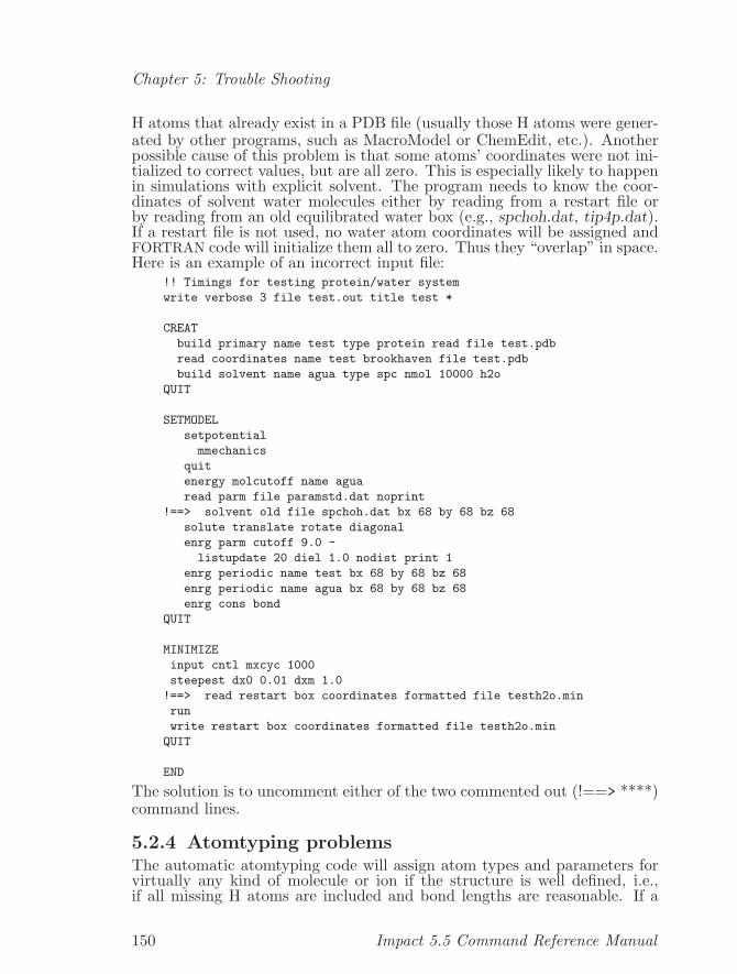
Chapter 5: Trouble Shooting
H atoms that already exist in a PDB file (usually those H atoms were gener-ated by other programs, such as MacroModel or ChemEdit, etc.). Anotherpossible cause of this problem is that some atoms’ coordinates were not ini-tialized to correct values, but are all zero. This is especially likely to happenin simulations with explicit solvent. The program needs to know the coor-dinates of solvent water molecules either by reading from a restart file orby reading from an old equilibrated water box (e.g., spchoh.dat, tip4p.dat).If a restart file is not used, no water atom coordinates will be assigned andFORTRAN code will initialize them all to zero. Thus they “overlap” in space.Here is an example of an incorrect input file:
!! Timings for testing protein/water system
write verbose 3 file test.out title test *
CREAT
build primary name test type protein read file test.pdb
read coordinates name test brookhaven file test.pdb
build solvent name agua type spc nmol 10000 h2o
QUIT
SETMODEL
setpotential
mmechanics
quit
energy molcutoff name agua
read parm file paramstd.dat noprint
!==> solvent old file spchoh.dat bx 68 by 68 bz 68
solute translate rotate diagonal
enrg parm cutoff 9.0 -
listupdate 20 diel 1.0 nodist print 1
enrg periodic name test bx 68 by 68 bz 68
enrg periodic name agua bx 68 by 68 bz 68
enrg cons bond
QUIT
MINIMIZE
input cntl mxcyc 1000
steepest dx0 0.01 dxm 1.0
!==> read restart box coordinates formatted file testh2o.min
run
write restart box coordinates formatted file testh2o.min
QUIT
END
The solution is to uncomment either of the two commented out (!==> ****)command lines.
5.2.4 Atomtyping problemsThe automatic atomtyping code will assign atom types and parameters forvirtually any kind of molecule or ion if the structure is well defined, i.e.,if all missing H atoms are included and bond lengths are reasonable. If a
150 Impact 5.5 Command Reference Manual
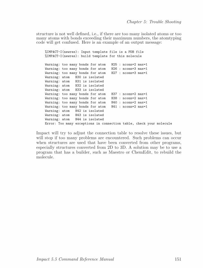
Chapter 5: Trouble Shooting
structure is not well defined, i.e., if there are too many isolated atoms or toomany atoms with bonds exceeding their maximum numbers, the atomtypingcode will get confused. Here is an example of an output message:
%IMPACT-I(newres): Input template file is a PDB file
%IMPACT-I(newres): build template for this molecule
Warning: too many bonds for atom H25 : nconn=2 max=1
Warning: too many bonds for atom H26 : nconn=3 max=1
Warning: too many bonds for atom H27 : nconn=3 max=1
Warning: atom H30 is isolated
Warning: atom H31 is isolated
Warning: atom H32 is isolated
Warning: atom H33 is isolated
Warning: too many bonds for atom H37 : nconn=2 max=1
Warning: too many bonds for atom H38 : nconn=2 max=1
Warning: too many bonds for atom H40 : nconn=2 max=1
Warning: too many bonds for atom H41 : nconn=2 max=1
Warning: atom H42 is isolated
Warning: atom H43 is isolated
Warning: atom H44 is isolated
Error: Too many exceptions in connection table, check your molecule
Impact will try to adjust the connection table to resolve these issues, butwill stop if too many problems are encountered. Such problems can occurwhen structures are used that have been converted from other programs,especially structures converted from 2D to 3D. A solution may be to use aprogram that has a builder, such as Maestro or ChemEdit, to rebuild themolecule.
Impact 5.5 Command Reference Manual 151

Chapter 5: Trouble Shooting
152 Impact 5.5 Command Reference Manual
Function Index
Function Index
(( ) . . . . . . . . . . . . . . . . . . . . . . . . . . . . . . . . . . 8
--1 . . . . . . . . . . . . . . . . . . . . . . . . . . . . . . . . . . 96-2 . . . . . . . . . . . . . . . . . . . . . . . . . . . . . . . . . . 96
[[ ] . . . . . . . . . . . . . . . . . . . . . . . . . . . . . . . . . . 8
11 . . . . . . . . . . . . . . . . . . . . . . . . . . . . . . . . . . . 96
22 . . . . . . . . . . . . . . . . . . . . . . . . . . . . . . . . . . . 96
Aaccuracy . . . . . . . . . . . . . . . . . . . . . . . . . . . . 38active . . . . . . . . . . . . . . . . . . . . . . . . . . . . . 111active_reg_incr . . . . . . . . . . . . . . . . . . . . 38actives [maestro | sd] afile fname
. . . . . . . . . . . . . . . . . . . . . . . . . . . 119, 120actxr . . . . . . . . . . . . . . . . . . . . . . . . . . . . . . 111actyr . . . . . . . . . . . . . . . . . . . . . . . . . . . . . . 111actzr . . . . . . . . . . . . . . . . . . . . . . . . . . . . . . 111agbnp . . . . . . . . . . . . . . . . . . . . . . . . . . . . . . . 32all . . . . . . . . . . . . . . . . . . . . . . . . . . . . . . . . . 26alldist . . . . . . . . . . . . . . . . . . . . . . . . . . . . 144allprint . . . . . . . . . . . . . . . . . . . . . . . . . . . 119alpha . . . . . . . . . . . . . . . . . . . . . . . . . . . . . . . 27amideoff . . . . . . . . . . . . . . . . . . . . . . . . . . . 113anneal . . . . . . . . . . . . . . . . . . . . . . . . . . . . . 105arrays . . . . . . . . . . . . . . . . . . . . . . . . . . . . . 136assign ligand . . . . . . . . . . . . . . . . . . . . . . . 70atname . . . . . . . . . . . . . . . . . . . . . . . . . . . . . . . 9
Bbaddist . . . . . . . . . . . . . . . . . . . . . . . . . . . . 117basis . . . . . . . . . . . . . . . . . . . . . . . . . . . . . . . 49best . . . . . . . . . . . . . . . . . . . . . . . . . . . . . . . 127bond . . . . . . . . . . . . . . . . . . . . . . . . . . . . . . . . 23
box . . . . . . . . . . . . . . . . . . . . . 84, 85, 111, 122boxxr . . . . . . . . . . . . . . . . . . . . . . . . . . . . . . 111boxyr . . . . . . . . . . . . . . . . . . . . . . . . . . . . . . 111boxzr . . . . . . . . . . . . . . . . . . . . . . . . . . . . . . 111bsize . . . . . . . . . . . . . . . . . . . . . . . . . . . . . . 110buffer . . . . . . . . . . . . . . . . . . . . . . . . . . . . . 112buffer_reg_size . . . . . . . . . . . . . . . . . . . . 38build . . . . . . . . . . . . . . . . . . . . . . . . . . . . . . . 17build primary check . . . . . . . . . . . . . . . . 96build primary type auto . . . . . . . . . . . . . 17build solvent . . . . . . . . . . . . . . . . . . . . . . . 20build types . . . . . . . . . . . . . . . . . . . . . . . . . 20by . . . . . . . . . . . . . . . . . . . . . . . . . . . . . . . . . 139by energy . . . . . . . . . . . . . . . . . . . . . . . . . . 125by glidescore . . . . . . . . . . . . . . . . . . 89, 125byspecies . . . . . . . . . . . . . . . . . . . . . . . 60, 65
Ccall . . . . . . . . . . . . . . . . . . . . . . . . . . . . . . . 145cavity_cutoff . . . . . . . . . . . . . . . . . . . . . . 31cdiel . . . . . . . . . . . . . . . . . . . . . . . . . . . . . . 107center read . . . . . . . . . . . . . . . . . . . . . . . . 111char . . . . . . . . . . . . . . . . . . . . . . . . . . . . . . . 143check . . . . . . . . . . . . . . . . . . . . . . . . . . . . . . . 18clean . . . . . . . . . . . . . . . . . . . . . . . . . . . . . . 116cmae . . . . . . . . . . . . . . . . . . . . . . . . . . . . . . . . 19cminit . . . . . . . . . . . . . . . . . . . . . . . . . . . . . 114cminit lig . . . . . . . . . . . . . . . . . . . . . . . . . 115cminit zero . . . . . . . . . . . . . . . . . . . . . . . . 115cntl. . . . . . . . . . . . . . . . . . . . . . . . . . . . . 60, 65collect . . . . . . . . . . . . . . . . . . . . . . . . . . . . 127concat . . . . . . . . . . . . . . . . . . . . . . . . . . . . . 143confgen . . . . . . . . . . . . . . . . . . . . . . . . 91, 117conjugate . . . . . . . . . . . . . . . . . . . . . . . . . . . 55consatom . . . . . . . . . . . . . . . . . . . . . . 101, 108consname . . . . . . . . . . . . . . . . . . . . . . . . . . . 108consolv [sgb] . . . . . . . . . . . . . . . . . . . . . . . 29consolv agbnp . . . . . . . . . . . . . . . . . . . . . . . 32consolv pbf . . . . . . . . . . . . . . . . . . . . . . . . . 30consolv pbf npsolv . . . . . . . . . . . . . . . . . . 35consolv sgb . . . . . . . . . . . . . . . . . . . . . . . . . 29constitle . . . . . . . . . . . . . . . . . . . . . . . . . 108constraints . . . . . . . . . . . . 23, 36, 101, 107convert . . . . . . . . . . . . . . . . . . . . . . . . . 62, 67corescale . . . . . . . . . . . . . . . . . . . . . . . . . 118create . . . . . . . . . . . . . . . . . . . . . . . . . . . . . . 17
Impact 5.5 Command Reference Manual 153
Function Index
csoft . . . . . . . . . . . . . . . . . . . . . . . . . . . . . . 105current . . . . . . . . . . . . . . . . . . . . . . . . . . . . 127cutoff. . . . . . . . . . . . . . . . . . . 25, 29, 31, 126cwall, csoft . . . . . . . . . . . . . . . . . . . . . . . 105cycgap . . . . . . . . . . . . . . . . . . . . . . . . . . . . . . 66cycrec . . . . . . . . . . . . . . . . . . . . . . . . . . . . . . 66
Ddebug . . . . . . . . . . . . . . . . . . . . . . . . . . . 30, 32delpose . . . . . . . . . . . . . . . . . . . . . . . . 89, 127delt. . . . . . . . . . . . . . . . . . . . . . . . . . . . . 61, 65deltae . . . . . . . . . . . . . . . . . . . . . . . . . . . . . . 56density . . . . . . . . . . . . . . . . . . . . . . . . . 39, 61DICE . . . . . . . . . . . . . . . . . . . . . . . . . . . . . . . 131dielco . . . . . . . . . . . . . . . . . . . . . . . . . 90, 123dielectric . . . . . . . . . . . . . . . . . . . . . . . . . 25distance . . . . . . . . . . . . . . . . . . . . . . . 25, 144dock . . . . . . . . . . . . . . . . . . . . . . . . . . . . . . . . 76DOCK . . . . . . . . . . . . . . . . . . . . . . . . . . . . . . . . 76dock_grid_size . . . . . . . . . . . . . . . . . . . . . 38docking . . . . . . . . . . . . . . . . . . . . . . . . . . . . . 76dvdp . . . . . . . . . . . . . . . . . . . . . . . . . . . . . . . . 61dx0 . . . . . . . . . . . . . . . . . . . . . . . . . . . . . . . . . 55dxm . . . . . . . . . . . . . . . . . . . . . . . . . . . . . . . . . 55dxm/ . . . . . . . . . . . . . . . . . . . . . . . . . . . . . . . . 55dynamics . . . . . . . . . . . . . . . . . . . . . . . . 57, 60
Eechooff . . . . . . . . . . . . . . . . . . . . . . . . . . . . . . 9echoon . . . . . . . . . . . . . . . . . . . . . . . . . . . . . . . 9ecut . . . . . . . . . . . . . . . . . . . . . . . . . . . 96, 117ecvdw . . . . . . . . . . . . . . . . . . . . . . . . . . . . . . . 90else . . . . . . . . . . . . . . . . . . . . . . . . . . . . . . . 144endif . . . . . . . . . . . . . . . . . . . . . . . . . . . . . . 144ENDWHILE . . . . . . . . . . . . . . . . . . . . . . . . . . . . 98energy . . . . . . . . . . . . . . . . . . . . . . . . . . . . . . 22epsout . . . . . . . . . . . . . . . . . . . . . . . . . . . . . . 38eq . . . . . . . . . . . . . . . . . . . . . . . . . . . . . . . . . 142every . . . . . . . . . . . . . . . . . . . . . . . . . . . 59, 71ewald . . . . . . . . . . . . . . . . . . . . . . . . . . . . . . . 27external . . . . . . . . . . . . . . . . . . . . . . . . . . . . 59external file . . . . . . . . . . . . . . . . . . . . . . 126
Ffast. . . . . . . . . . . . . . . . . . . . . . . . . . . . . 62, 67featurefile . . . . . . . . . . . . . . . . . . . . . . . 108featverb . . . . . . . . . . . . . . . . . . . . . . . . . . . 109file . . . . . . . . . . . . . . . . . . . . . . . . . . 8, 23, 71
final . . . . . . . . . . . . . . . . . . . . . . . . . . 85, 124finalonly . . . . . . . . . . . . . . . . . . . . . . . . . 109flex . . . . . . . . . . . . . . . . . . . . . . . . . . . 91, 123fmm . . . . . . . . . . . . . . . . . . . . . . . . . . . . . . . . . 28fobo. . . . . . . . . . . . . . . . . . . . . . . . . . . . . 19, 21force . . . . . . . . . . . . . . . . . . . . . . . . . . . . . . . 27formatted . . . . . . . . . . . . . . . . . . . . . . . . . . . 59forspecies . . . . . . . . . . . . . . . . . . . . . . 60, 65fos . . . . . . . . . . . . . . . . . . . . . . . . . . . . . . 19, 21fresidue . . . . . . . . . . . . . . . . . . . . . . . . . . . . . 9ftol . . . . . . . . . . . . . . . . . . . . . . . . . . . . . . . 123functions . . . . . . . . . . . . . . . . . . . . . . . . . 139
Gge . . . . . . . . . . . . . . . . . . . . . . . . . . . . . . . . . 142Glide . . . . . . . . . . . . . . . . . . . . . . . . . . . . . . . 76GLIDE . . . . . . . . . . . . . . . . . . . . . . . . . . . . . . . 76goto . . . . . . . . . . . . . . . . . . . . . . . . . . . . . . . 145GOTO ABORT . . . . . . . . . . . . . . . . . . . . . . . . . . 97GOTO BREAK . . . . . . . . . . . . . . . . . . . . . . . . . . 97gotostruct . . . . . . . . . . . . . . . . . . . . . . . . . 19gotostruct ’startlig’ . . . . . . . . . . . . . . 97grdist . . . . . . . . . . . . . . . . . . . . . . . . . . . . . 144greedy . . . . . . . . . . . . . . . . . . . . . . 78, 84, 122grid_size . . . . . . . . . . . . . . . . . . . . . . . . . . . 38gt . . . . . . . . . . . . . . . . . . . . . . . . . . . . . . . . . 142
Hh2o . . . . . . . . . . . . . . . . . . . . . . . . . . . . . . . . . 20hbfilt . . . . . . . . . . . . . . . . . . . . . . . . . . . . . . 90hbpenal . . . . . . . . . . . . . . . . . . . . . . . . . . . . . 90high_res . . . . . . . . . . . . . . . . . . . . . . . . . . . . 32highacc . . . . . . . . . . . . . . . . . . . . . . . . . . . . 124histogram . . . . . . . . . . . . . . . . . . . . . . . . . 143hmass . . . . . . . . . . . . . . . . . . . . . . . . . . . . . . . 26HMC . . . . . . . . . . . . . . . . . . . . . . . . . . . . . . . . . 64hydrogen_radius . . . . . . . . . . . . . . . . . . . . 38
Iif . . . . . . . . . . . . . . . . . . . . . . . . . . . . . . . . . 144IF ’buildcheck’ LT 0 . . . . . . . . . . . . 96, 97ifo . . . . . . . . . . . . . . . . . . . . . . . . . . . . . . 19, 21Impact output of Glide . . . . . . . . . . . . . 128inactives [maestro | sd] ifile fname
. . . . . . . . . . . . . . . . . . . . . . . . . . . . . . . 119init . . . . . . . . . . . . . . . . . . . . . . . . . . . . . . . 114
154 Impact 5.5 Command Reference Manual
Function Index
init rand [cmrange val] [thetarange
val] [phirange val] [psirange
val] [seed num] . . . . . . . . . . . . . . . 114init read xcm val ycm val zcm val phi
val theta val psi val . . . . . . . . . 114init zero . . . . . . . . . . . . . . . . . . . . . . . . . . 114input . . . . . . . . . . . . . . . . . . . . . . . . . . . 60, 65input cntl . . . . . . . . . . . . . . . . . . . . . . . . . . 71intermolecular . . . . . . . . . . . . . . . . . . . . . 36intramolecular . . . . . . . . . . . . . . . . . . . . . 36itmax . . . . . . . . . . . . . . . . . . . . . . . . . . . . . . . 90
Jjrate . . . . . . . . . . . . . . . . . . . . . . . . . . . . . . . 66jtemp . . . . . . . . . . . . . . . . . . . . . . . . . . . . . . . 66jwalk . . . . . . . . . . . . . . . . . . . . . . . . . . . . . . . 66
Kkeep . . . . . . . . . . . . . . . . . . . . . . . 39, 113, 127keywords . . . . . . . . . . . . . . . . . . . . . . . . . . . . . 7kmax . . . . . . . . . . . . . . . . . . . . . . . . . . . . . . . . 27
Lle . . . . . . . . . . . . . . . . . . . . . . . . . . . . . . . . . 142level . . . . . . . . . . . . . . . . . . . . . . . . . . . . . . . 28lewis . . . . . . . . . . . . . . . . . . . . . . . . . . . 19, 21LIA . . . . . . . . . . . . . . . . . . . . . . . . . . . . . . . . . 68ligand . . . . . . . . . . . . . . . . . . . . . . . . . 87, 113ligand keep . . . . . . . . . . . . . . . . . . . . . . . . . 90ligand name lig . . . . . . . . . . . . . . . . . . . . . 89lists . . . . . . . . . . . . . . . . . . . . . . . . . 132, 146listupdate . . . . . . . . . . . . . . . . . . . . . . . . . 25loosedock . . . . . . . . . . . . . . . . . . . . . . . . . 109loosegrid . . . . . . . . . . . . . . . . . . . . . . . . . 109low_res . . . . . . . . . . . . . . . . . . . . . . . . . . . . . 31lresidue . . . . . . . . . . . . . . . . . . . . . . . . . . . . . 9LRM . . . . . . . . . . . . . . . . . . . . . . . . . . . . . . . . . 68lstdist . . . . . . . . . . . . . . . . . . . . . . . . . . . . 144lt . . . . . . . . . . . . . . . . . . . . . . . . . . . . . . . . . 142
Mmaestro . . . . . . . . . . . . . . . . . . . . . . . . . . . . . 18maxconf . . . . . . . . . . . . . . . . . . . . . . . . . . . . 116maxcore . . . . . . . . . . . . . . . . . . . . . . . . . . . . 117maxhard . . . . . . . . . . . . . . . . . . . . . . . . . . . . 124maxit . . . . . . . . . . . . . . . . . . . . . . . . . . . . . . . 55maxiter . . . . . . . . . . . . . . . . . . . . . . . . . . . . . 23
maxkeep . . . . . . . . . . . . . . . . . . . . . . . . 88, 121maxperlig . . . . . . . . . . . . . . . . . . . . . . 89, 126maxpole . . . . . . . . . . . . . . . . . . . . . . . . . . . . . 28maxref . . . . . . . . . . . . . . . . . . . . . . . . . . . . . . 90maxsoft . . . . . . . . . . . . . . . . . . . . . . . . . . . . 124med_res . . . . . . . . . . . . . . . . . . . . . . . . . . . . . 32medium . . . . . . . . . . . . . . . . . . . . . . . . . . 62, 67metalbind [DEPRECATED] . . . . . . . . . . . . 110metalfilt . . . . . . . . . . . . . . . . . . . . . . . . . . . 90metric . . . . . . . . . . . . . . . . . . . . . . . . . . . . . . 66min_grid_size . . . . . . . . . . . . . . . . . . . . . . 38minimize . . . . . . . . . . . . . . . . 57, 79, 90, 123minstep . . . . . . . . . . . . . . . . . . . . . . . . . . . . . 66mixture . . . . . . . . . . . . . . . . . . . . . . . . . . . . . 38mmechanics . . . . . . . . . . . . . . . . . . . . . . . . . 26molcutoff . . . . . . . . . . . . . . . . . . . . . . . . . . . 22mole . . . . . . . . . . . . . . . . . . . . . . . 18, 107, 113montecarlo . . . . . . . . . . . . . . . . . . . . . . . . . 57multiple . . . . . . . . . . . . . . . . . . . . . . . . . . . 113mxcyc . . . . . . . . . . . . . . . . . . . . . . . . . . . 56, 65
Nname . . . . . . . . . . . . . . . . . . . . . 9, 18, 107, 113name lig . . . . . . . . . . . . . . . . . . . . . . . . . . . . 96name recep . . . . . . . . . . . . . . . . . . . . . . . . . . 82ncon . . . . . . . . . . . . . . . . . . . . . . . . . . . . . . . . 37ncons . . . . . . . . . . . . . . . . . . . . . . . . . 101, 107ncycle val . . . . . . . . . . . . . . . . . . . . . . . . . 124new . . . . . . . . . . . . . . . . . . . . . . . . . . . . . . . . 115nextstruct . . . . . . . . . . . . . . . . . . . . . . 19, 97nfill [DEPRECATED] . . . . . . . . . . . . . . . . 110nfull . . . . . . . . . . . . . . . . . . . . . . . . . . . . . . . 56nhscale . . . . . . . . . . . . . . . . . . . . . . . . . . . . . 56nlev . . . . . . . . . . . . . . . . . . . . . . . . . . . . . . . 111nmdmc . . . . . . . . . . . . . . . . . . . . . . . . . . . . . . . 65no14 . . . . . . . . . . . . . . . . . . . . . . . . . . . . . . . . 27noangle . . . . . . . . . . . . . . . . . . . . . . . . . . . . . 27nobond . . . . . . . . . . . . . . . . . . . . . . . . . . . . . . 27nodistance . . . . . . . . . . . . . . . . . . . . . . . . . 25noecons . . . . . . . . . . . . . . . . . . . . . . . . . . . . . 27noel . . . . . . . . . . . . . . . . . . . . . . . . . . . . . . . . 27noel14 . . . . . . . . . . . . . . . . . . . . . . . . . . . . . . 27noelec . . . . . . . . . . . . . . . . . . . . . . . . . . . . . 115noforce . . . . . . . . . . . . . . . . . . . . . . . . . . . . . 27nohb . . . . . . . . . . . . . . . . . . . . . . . . . . . . . . . . 27noprint . . . . . . . . . . . . . . . . . . . . . . . . . . . . 120norecep . . . . . . . . . . . . . . . . . . . . . . . . . . . . 126noringconf . . . . . . . . . . . . . . . . . . . . . . . . 118norot . . . . . . . . . . . . . . . . . . . . . . . . . . . . . . 115noscore . . . . . . . . . . . . . . . . . . . . . . . . 90, 121
Impact 5.5 Command Reference Manual 155
Function Index
notail . . . . . . . . . . . . . . . . . . . . . . . . . . . . . . 27notestff . . . . . . . . . . . . . . . . . . . . . . . . . . . . 19notors . . . . . . . . . . . . . . . . . . . . . . . . . . . . . . 27novdw . . . . . . . . . . . . . . . . . . . . . . . . . . . . . . . 27nphobic num file fname . . . . . . . . . . . . 107nposit . . . . . . . . . . . . . . . . . . . . . . . . . . . . . 108nprnt . . . . . . . . . . . . . . . . . . . . . . . . . . . 61, 65npsolv . . . . . . . . . . . . . . . . . . . . . . . . . . . . . . 29nreport . . . . . . . . . . . . . . . . . . . . . . . . 89, 126nsec . . . . . . . . . . . . . . . . . . . . . . . . . . . 37, 112nstep . . . . . . . . . . . . . . . . . . . . . . . . . . . . . . . 61nusecons [DEPRECATED] . . . . . . . . . . . . . 110nusephob [DEPRECATED] . . . . . . . . . . . . . 110
Ooperations . . . . . . . . . . . . . . . . . . . . . . . . 139OPLS . . . . . . . . . . . . . . . . . . . . . . . . . . . . . . . . 15OPLS-AA . . . . . . . . . . . . . . . . . . . . . . . . . . . . . 20OPLS2001 . . . . . . . . . . . . . . . . . . . . . . . . . . . . 15OPLS2005 . . . . . . . . . . . . . . . . . . . . . . . . . . . . 15outcutoff . . . . . . . . . . . . . . . . . . . . . . . . . . . 26outlistupdate . . . . . . . . . . . . . . . . . . . . . . 26overlap . . . . . . . . . . . . . . . . . . . . . . . . . . . . . 39
Pparam (Liaison) . . . . . . . . . . . . . . . . . . . . 71parameter . . . . . . . . . . . . . . . . . . . 85, 88, 116parameter clean final . . . . . . . . . . . . . . 91parm . . . . . . . . . . . . . . . . . . . . . . . . . . . . . . . . 25patype . . . . . . . . . . . . . . . . . . . . . . . . . . . . . . 21pbf . . . . . . . . . . . . . . . . . . . . . . . . . . . . . . . . . 30pbfevery . . . . . . . . . . . . . . . . . . . . . . . . . . . . 31pdb . . . . . . . . . . . . . . . . . . . . . . . . . . . . . . . . . 18penalty val lowsim val highsim val
. . . . . . . . . . . . . . . . . . . . . . . . . . . . . . . 120percent val . . . . . . . . . . . . . . . . . . . . . . . 119periodic . . . . . . . . . . . . . . . . . . . . . . . . . . . . 22pff . . . . . . . . . . . . . . . . . . . . . . . . . . . . . . . . . 35plewis . . . . . . . . . . . . . . . . . . . . . . . . . . . . . . 21pparam . . . . . . . . . . . . . . . . . . . . . . . . . . . . . . 21print . . . . . . . . . . . . . . . . . . . . . . . . . . . . . . . 26printe . . . . . . . . . . . . . . . . . . . . . . . . . . . . . . 38printf . . . . . . . . . . . . . . . . . . . . . . . . . . . . . . 38protvdwscale . . . . . . . . . . . . . . . . . . . . . . . 83put . . . . . . . . . . . . . . . . . . . . . . . . . . . . . . . . 138PUT ’i’ + 1 INTO ’i’ . . . . . . . . . . . . . . . . . 98PUT ’startlig’ INTO ’i’ . . . . . . . . . . . . . 97
QQMMM . . . . . . . . . . . . . . . . . . . . . . . . . . . . . . . . 44qmregion . . . . . . . . . . . . . . . . . . . . . . . . . . . . 44qmtransition . . . . . . . . . . . . . . . . . . . . . . . 51
Rrand . . . . . . . . . . . . . . . . . . . . . . . . . . . . . . . 143range . . . . . . . . . . . . . . . . . . . . . . . . . . . . . . . 37RATTLE . . . . . . . . . . . . . . . . . . . . . . . . . . 61, 65rdiel . . . . . . . . . . . . . . . . . . . . . . . . . . . . . . 107read . . . . . . . . . . . . . . . . . . 23, 26, 57, 62, 67readf . . . . . . . . . . . . . . . . . . . . . . . . . . . . . . 106readgreed . . . . . . . . . . . . . . . . . . . . . . 88, 122readscreen . . . . . . . . . . . . . . . . . . . . . 88, 121readsurface . . . . . . . . . . . . . . . . . . . . . . . 112recep . . . . . . . . . . . . . . . . . . . . . . . . . . . . . . 126receptor . . . . . . . . . . . . . . . . . . . . 82, 87, 106reference . . . . . . . . . . . . . . . . . . . . . 114, 127refine . . . . . . . . . . . . . . . . . . . . . . 79, 90, 123reject val . . . . . . . . . . . . . . . . . . . . . . . . . 120relax . . . . . . . . . . . . . . . . . . . . . . . . . . . 61, 65report . . . . . . . . . . . . . . . . . . . . . . . . . 88, 125report ... write filename ... . . . . . . 91report collect. . . . . . . . . . . . . . . . . . . . . . 90rescutoff . . . . . . . . . . . . . . . . . . . . . . . . . . . 22resnumber . . . . . . . . . . . . . . . . . . . . . . . . . . . . 9rest . . . . . . . . . . . . . . . . . . . . . . . . . . . . . . . . 55restcoef . . . . . . . . . . . . . . . . . . . . . . . . . . . 108restexp . . . . . . . . . . . . . . . . . . . . . . . . . . . . 108restore . . . . . . . . . . . . . . . . . . . . . . . . . . . . 143return . . . . . . . . . . . . . . . . . . . . . . . . . . . . . 145rmscut . . . . . . . . . . . . . . . . . . . . . . . . . . . . . . 56rmspose . . . . . . . . . . . . . . . . . . . . . . . . 89, 127rotations . . . . . . . . . . . . . . . . . . . . . . . 61, 66rpos . . . . . . . . . . . . . . . . . . . . . . . . . . . . . . . 108rrespa . . . . . . . . . . . . . . . . . . . . . . . . . . 62, 67run . . . . . . . . . . . . . . . . . . 57, 62, 67, 85, 128
Ssample . . . . . . . . . . . . . . . . . . . . . . . . . . . . . . 71sampling . . . . . . . . . . . . . . . . . . . . . . . . . . . 124save . . . . . . . . . . . . . . . . . . . . . . . . . . . . . . . 116scbsize . . . . . . . . . . . . . . . . . . . . . . . . . . . . 121scorecut . . . . . . . . . . . . . . . . . . . . . . . 88, 121scoring . . . . . . . . . . . . . . . . . . . . . . . . 90, 124scr14 . . . . . . . . . . . . . . . . . . . . . . . . . . . . . . . 25screen . . . . . . . . . . . . 77, 84, 88, 89, 90, 121scut . . . . . . . . . . . . . . . . . . . . . . . . . . . . . . . 111
156 Impact 5.5 Command Reference Manual
Function Index
sd . . . . . . . . . . . . . . . . . . . . . . . . . . . . . . . . . . 18seed. . . . . . . . . . . . . . . . . . . . . . . . . . . . . 61, 65set . . . . . . . . . . . . . . . . . . . . . . . . . . . . . . . . . 15Set ffield . . . . . . . . . . . . . . . . . . . . . . . . . . 15Set force . . . . . . . . . . . . . . . . . . . . . . . . . . . 15Set Noinvalidate . . . . . . . . . . . . . . . . . . . 16set path . . . . . . . . . . . . . . . . . . . . . . . . . . . . 15setmodel . . . . . . . . . . . . . . . . . . . . . . . . . . . . 21setpotential . . . . . . . . . . . . . . . . . . . . . . . 26setup . . . . . . . . . . . . . . . . . . . . . . 89, 116, 125sgb . . . . . . . . . . . . . . . . . . . . . . . . . . . . . . . . . 29sgbp . . . . . . . . . . . . . . . . . . . . . . . . . . . . . . . . 37SHAKE . . . . . . . . . . . . . . . . . . . . . . . . . . . 61, 65simil . . . . . . . . . . . . . . . . . . . . . . . . . . . . . . 118singlep . . . . . . . . . . . . . . . . . . . . . . . . . . . . . 99skipb n . . . . . . . . . . . . . . . . . . . . . . . . . . . . 121smooth . . . . . . . . . . . . . . . . . . . . . 82, 104, 143smooth anneal 2 . . . . . . . . . . . . . . . . . . . . . 90smoothing . . . . . . . . . . . . . . . . . . . . . . . . . . . 28solute . . . . . . . . . . . . . . . . . . . . . . . . . . 38, 39solvent . . . . . . . . . . . . . . . . . . . . . . . . . 20, 38spawn . . . . . . . . . . . . . . . . . . . . . . . . . . . . . . 145spc . . . . . . . . . . . . . . . . . . . . . . . . . . . . . . . . . 20statistics . . . . . . . . . . . . . . . . . . . . . . 61, 66statistics off . . . . . . . . . . . . . . . . . . 61, 66statistics on . . . . . . . . . . . . . . . . . . . 61, 66stdrot . . . . . . . . . . . . . . . . . . . . . . . . . . . . . 115steepest . . . . . . . . . . . . . . . . . . . . . . . . . . . . 55stop. . . . . . . . . . . . . . . . . . . . . . . . . . . . . 61, 66stop rotations . . . . . . . . . . . . . . . . . . 61, 66swalk . . . . . . . . . . . . . . . . . . . . . . . . . . . . . . . 66
Ttagged . . . . . . . . . . . . . . . . . . . . . . . . . . . . . . 18tail . . . . . . . . . . . . . . . . . . . . . . . . . . . . . . . . 27target . . . . . . . . . . . . . . . . . . . . . . . . . . 61, 66taup . . . . . . . . . . . . . . . . . . . . . . . . . . . . . . . . 61testff . . . . . . . . . . . . . . . . . . . . . . . . . . . . . . 19tip4p . . . . . . . . . . . . . . . . . . . . . . . . . . . . . . . 20tips . . . . . . . . . . . . . . . . . . . . . . . . . . . . . . . . 20tncut . . . . . . . . . . . . . . . . . . . . . . . . . . . . . . . 56tnewton . . . . . . . . . . . . . . . . . . . . . . . . . . . . . 56tol . . . . . . . . . . . . . . . . . . . . . . . . . . . . . . 61, 65tphi . . . . . . . . . . . . . . . . . . . . . . . . . . . . . . . . 37tpsi . . . . . . . . . . . . . . . . . . . . . . . . . . . . . . . . 37Types . . . . . . . . . . . . . . . . . . . . . . . . . . . . . . . 20
Uunformatted . . . . . . . . . . . . . . . . . . . . . . . . 59usecons [DEPRECATED] . . . . . . . . . . . . . . 110usephob [DEPRECATED] . . . . . . . . . . . . . . 110
Vvariables . . . . . . . . . . . . . . . . . . . . . . . . . . . . 7verbose . . . . . . . . . . . . . . . . . . . . . . . . . . . . . . 6verbosity . . . . . . . . . . . . . . . . . . . . . . . . . 116verlet . . . . . . . . . . . . . . . . . . . . . . . . . . 62, 67vsoft . . . . . . . . . . . . . . . . . . . . . . . . . . . . . . 105
Wweight constraints . . . . . . . . . . . . . . . . . 36weight intermolecular . . . . . . . . . . . . . . 36weight intramolecular . . . . . . . . . . . . . . 36wfile fname . . . . . . . . . . . . . . . . . . . 119, 120while . . . . . . . . . . . . . . . . . . . . . . . . . . . . . . 144WHILE (’endlig’ LT 1 OR ’i’ LE
’endlig’) . . . . . . . . . . . . . . . . . . . . . . 97with . . . . . . . . . . . . . . . . . . . . . . . . . . . . . . . 138withonly . . . . . . . . . . . . . . . . . . . . . . . . . . . 138without . . . . . . . . . . . . . . . . . . . . . . . . . . . . 138write . . . . . . . . . . . . . . . . . . . . . . . . 57, 62, 67write filename fname . . . . . . . . . . . . . . 127writecdie . . . . . . . . . . . . . . . . . . . . . . . . . 107writecmsite . . . . . . . . . . . . . . . . . . . . . . . 122writef . . . . . . . . . . . . . . . . . . . . . . . . . . . . . 106writef 1ets_single_grid . . . . . . . . . . . . 83writegreed . . . . . . . . . . . . . . . . . . . . . 85, 122writerdie . . . . . . . . . . . . . . . . . . . . . . . . . 107writescreen . . . . . . . . . . . . . . . . . . . . 85, 121writesurface . . . . . . . . . . . . . . . . . . . . . . 112
Xxpos . . . . . . . . . . . . . . . . . . . . . . . . . . . . . . . 108
Yypos . . . . . . . . . . . . . . . . . . . . . . . . . . . . . . . 108
Zzonecons . . . . . . . . . . . . . . . . . . . . . . . . . . . . 40zpos . . . . . . . . . . . . . . . . . . . . . . . . . . . . . . . 108
Impact 5.5 Command Reference Manual 157

Function Index
158 Impact 5.5 Command Reference Manual
Concept Index
Concept Index
AActive site . . . . . . . . . . . . . . . . . . . . . . . . . 106Adaptive grid . . . . . . . . . . . . . . . . . . . . . . 106Adding long-range corrections . . . . . . . . 27Advanced Scripts . . . . . . . . . . . . . . . . . . . 144AGBNP implicit solvent model . . . . . . . 32Arithmetic operations . . . . . . . . . . . . . . . 139Atom Types, automatic generation of
atom types . . . . . . . . . . . . . . . . . . . . . . 20Atom types, printing . . . . . . . . . . . . . . . . . 21Atoms, specifying . . . . . . . . . . . . . . . . . . . . . 9Authors of Impact . . . . . . . . . . . . . . . . . . . . 1
BBackground in Impact . . . . . . . . . . . . . . 131Binding energy prediction, Liaison . . . . 74Bond constraints . . . . . . . . . . . . . . . . . . . . . 23Bond distance . . . . . . . . . . . . . . . . . . . . . . 144Boolean operators . . . . . . . . . . . . . . . . . . 142Buffering atoms/regions . . . . . . . . . . . . . . 40Building the molecular structure of the
solvent . . . . . . . . . . . . . . . . . . . . . . . . . . 20Building the simulation system . . . . . . . 17By, function mapping . . . . . . . . . . . . . . . 139
CCalling subroutines . . . . . . . . . . . . . . . . . 145Collecting statistics . . . . . . . . . . . . . . . 61, 66Colon notation . . . . . . . . . . . . . . . . . . . . . 136Command language . . . . . . . . . . . . . . . . . 131Comments in the input file . . . . . . . . . . . . 7Communication between docking and
other tasks . . . . . . . . . . . . . . . . . . . . . 125Conformation generation for docking
. . . . . . . . . . . . . . . . . . . . . . . . . . . . . . . 117Conjugate gradient. . . . . . . . . . . . . . . . . . . 55Constant energy simulations . . . . . . . . . . 61Constant pressure simulations . . . . . 27, 60Constant temperature simulations . . . . . 61Constant volume simulations . . . . . . . . . 60Constraint regions . . . . . . . . . . . . . . . . . . . 40Constraints . . . . . . . . . . . . . . . . . . . . . . 61, 65Constraints, bonds or distances . . . . . . . 23Constraints, distance and torsional . . . . 36
Constraints, Glide . . . . . . . . . . . . . . 101, 107Constructs, programming . . . . . . . . . . . . 144continuum solvent models . . . . . 29, 30, 32Converting trajectories between the old
and the new formats. . . . . . . . . . 62, 67Coordinates, reading and writing . . . . . . 57Coulomb-vdW interaction energy, Glide
. . . . . . . . . . . . . . . . . . . . . . . . . . . . 79, 123Create task . . . . . . . . . . . . . . . . . . . . . . . . . . 17Cutoff, molecular . . . . . . . . . . . . . . . . . . . . 22Cutoff, residue-based . . . . . . . . . . . . . . . . . 22Cutoffs . . . . . . . . . . . . . . . . . . . . . . . . . . . . . . 25Cutoffs, read . . . . . . . . . . . . . . . . . . . . . . . . 25
DData directories . . . . . . . . . . . . . . . . . . . . . 15Data representation . . . . . . . . . . . . . . . . . . 59Data structures, lists . . . . . . . . . . . . . . . . 132Decision making . . . . . . . . . . . . . . . . . . . . 144Defining the model potential . . . . . . . . . . 26Dependencies, machine . . . . . . . . . . . . . . . 59DICE . . . . . . . . . . . . . . . . . . . . . . . . . . . . . . 131Dielectric constant . . . . . . . . . . . . . . . . . . . 25Disposition of arrays . . . . . . . . . . . . . . . . 116Distance constraints . . . . . . . . . . . . . . 23, 36Distance, bond . . . . . . . . . . . . . . . . . . . . . 144Distance-dependent dielectric . . . . . . . . . 25Distances between sets of points . . . . . 144DOCK task . . . . . . . . . . . . . . . . . . . . . . . . . 76Docking a single conformation . . . . . . . . 86Docking grid setup . . . . . . . . . . . . . . . . . . . 80Docking multiple ligands . . . . . . . . . . . . . 91Docking task . . . . . . . . . . . . . . . . . . . . . . . . 76Docking, communication with other tasks
. . . . . . . . . . . . . . . . . . . . . . . . . . . . . . . 125Docking, conformation generation for
. . . . . . . . . . . . . . . . . . . . . . . . . . . . . . . 117Docking, output of . . . . . . . . . . . . . . . . . . 128Docking, reporting results of . . . . . . . . . 125Docking, running the calculation . . . . . 128Docking, similarity scoring for . . . . . . . 118Docking, smoothing functions for . . . . 104Docking, specifying minimization phase of
. . . . . . . . . . . . . . . . . . . . . . . . . . . . . . . 123Docking, specifying parameters for . . . 116
Impact 5.5 Command Reference Manual 159
Concept Index
Docking, specifying screening phase of. . . . . . . . . . . . . . . . . . . . . . . . . . . . . . . 121
Docking, specifying the ligand for . . . . 113Docking, specifying the receptor for . . 106Documentation, online . . . . . . . . . . . . . . . 14Dynamics task . . . . . . . . . . . . . . . . . . . . . . . 60Dynamics, input control parameters . . . 60Dynamics, read . . . . . . . . . . . . . . . . . . . . . . 62Dynamics, run . . . . . . . . . . . . . . . . . . . . . . . 62Dynamics, write . . . . . . . . . . . . . . . . . . . . . 62
EEnergies, printing the . . . . . . . . . . . . . . . . 26Energy parameters, reading . . . . . . . . . . . 22Ewald summation . . . . . . . . . . . . . . . . 27, 28Examining skipped rough-score sites . . 79,
123
FFast Multipole Method . . . . . . . . 25, 27, 28Files, specifying . . . . . . . . . . . . . . . . . . . . . . . 8Filters and parameters for Glide scoring
function . . . . . . . . . . . . . . . . . . . . . . . 124Flexible docking . . . . . . . . . . . . . . . . . . . . . 91Flow control . . . . . . . . . . . . . . . . . . . . . . . . 144FMM . . . . . . . . . . . . . . . . . . . . . . . . 25, 27, 28Force field . . . . . . . . . . . . . . . . . . . . . . . . . . . 15Force field terms, printing . . . . . . . . . . . . 21Force field, setting . . . . . . . . . . . . . . . . . . . 15Freezing atoms/regions . . . . . . . . . . . . . . . 40Function mapping . . . . . . . . . . . . . . . . . . 139Functions in Impact . . . . . . . . . . . . . . . . . 139Functions, applying over lists . . . . . . . . 139
GGeneralized Born solvent model . . . . . . . 29Glide constraints . . . . . . . . . . . . . . . 101, 107Glide energy minimization . . . . . . . 79, 123Glide greedy scoring . . . . . . . . . . . . . 78, 122Glide pose refinement . . . . . . . . . . . . 79, 123Glide pose screening . . . . . . . . . . . . . 77, 121Glide rough scoring . . . . . . . . . . . . . . 77, 121Glide, communication with other tasks
. . . . . . . . . . . . . . . . . . . . . . . . . . . . . . . 125Glide, conformation generation for . . . 117Glide, extra precision . . . . . . . . . . . . . . . 124Glide, final scoring . . . . . . . . . . . . . . . . . . 124Glide, flexible docking . . . . . . . . . . . . . . . . 91
Glide, grid setup for . . . . . . . . . . . . . . . . . 80Glide, ligand recycling . . . . . . . . . . . . . . 124Glide, multiple ligands . . . . . . . . . . . . . . . 91Glide, output of . . . . . . . . . . . . . . . . . . . . 128Glide, penalizing amide rotations . . . . 113Glide, reporting results of . . . . . . . . . . . 125Glide, requiring specific interactions
. . . . . . . . . . . . . . . . . . . . . . . . . . . 101, 107Glide, rigid docking . . . . . . . . . . . . . . . . . . 86Glide, running the calculation . . . . . . . 128Glide, scoring input structure(s) . . . . . . 99Glide, similarity scoring for . . . . . . . . . . 118Glide, single ligand . . . . . . . . . . . . . . . . . . 86Glide, smoothing functions for . . . . . . . 104Glide, specifying minimization phase of
. . . . . . . . . . . . . . . . . . . . . . . . . . . . . . . 123Glide, specifying parameters for . . . . . . 116Glide, specifying screening phase of . . 121Glide, specifying the ligand for . . . . . . . 113Glide, specifying the receptor for . . . . . 106Glide, turning off amide rotations . . . . 113GlideScore . . . . . . . . . . . . . . . . . . . . . . . . . 124Goto, transfer of control . . . . . . . . . . . . . 145Greedy scoring, Glide . . . . . . . . . . . . 78, 122Grid box . . . . . . . . . . . . . . . . . . . . . . . . . . . 106Grid energy minimization, Glide . . 79, 123Grid setup for Glide . . . . . . . . . . . . . . . . . 80
HHMC task . . . . . . . . . . . . . . . . . . . . . . . . . . . 64HMC, input control parameters . . . . . . . 65HMC, read . . . . . . . . . . . . . . . . . . . . . . . . . . 67HMC, run . . . . . . . . . . . . . . . . . . . . . . . . . . . 67HMC, write . . . . . . . . . . . . . . . . . . . . . . . . . 67Hybrid Monte Carlo, HMC . . . . . . . . . . . 64Hyphen notation . . . . . . . . . . . . . . . . . . . . 137
Iif/else/endif . . . . . . . . . . . . . . . . . . . . . . . . 144Impact Background . . . . . . . . . . . . . . . . . 131Initial array sizes . . . . . . . . . . . . . . . . . . . 116Initial pose . . . . . . . . . . . . . . . . . . . . . . . . . 113Input control parameters for dynamics
. . . . . . . . . . . . . . . . . . . . . . . . . . . . . . . . 60Input control parameters for HMC . . . . 65Input files, reading . . . . . . . . . . . . . . . . . . . . 5Input scripting language . . . . . . . . . . . . . 131installation . . . . . . . . . . . . . . . . . . . . . . . . . . . 3Integrator, multiple-time step . . . . . 62, 67
160 Impact 5.5 Command Reference Manual
Concept Index
Integrator, r-RESPA . . . . . . . . . . . . . . 62, 67Integrator, Verlet . . . . . . . . . . . . . . . . . 62, 67Internal lists . . . . . . . . . . . . . . . . . . . . . . . . 133
JJ-Walking . . . . . . . . . . . . . . . . . . . . . . . . . . . 64
LLewis structure checking/refinement . . 19,
21Liaison . . . . . . . . . . . . . . . . . . . . . . . . . . . . . . 68Liaison, assigning ligand . . . . . . . . . . . . . . 70Liaison, binding energy prediction . . . . . 74Liaison, fitting . . . . . . . . . . . . . . . . . . . . . . . 72Liaison, general overview . . . . . . . . . . . . . 68Liaison, input control parameters . . . . . 71Liaison, parameters . . . . . . . . . . . . . . . . . . 71Liaison, prediction . . . . . . . . . . . . . . . . . . . 74Liaison, selecting sampling method . . . . 71Liaison, simulation . . . . . . . . . . . . . . . . . . . 72Ligand-receptor docking . . . . . . . . . . . . . . 76Linear Interaction Approximation (LIA)
. . . . . . . . . . . . . . . . . . . . . . . . . . . . . . . . 68Linear Response Method (LRM) . . . . . . 68List operators . . . . . . . . . . . . . . . . . . . . . . 143List selection . . . . . . . . . . . . . . . . . . . . . . . 138List subsets . . . . . . . . . . . . . . . . . . . . 135, 138Lists as data structures . . . . . . . . . . . . . 132Lists as parameters . . . . . . . . . . . . . . . . . 146Lists, creating . . . . . . . . . . . . . . . . . . . . . . 138Lists, internal . . . . . . . . . . . . . . . . . . . . . . 133
MMachine dependencies . . . . . . . . . . . . . . . . 59Maestro files, writing . . . . . . . . . . . . . . . . . 57Maestro properties, retaining . . . . . . . . . 16Mapping of functions over lists . . . . . . . 139mass, hydrogen atoms . . . . . . . . . . . . . . . . 26Math functions . . . . . . . . . . . . . . . . . . . . . 139Max/min distance between sets of points
. . . . . . . . . . . . . . . . . . . . . . . . . . . . . . . 144Minimization, beginning . . . . . . . . . . . . . . 57Minimization, conjugate gradient . . . . . . 55Minimization, output frequency . . . . . . . 55Minimization, steepest descent . . . . . . . . 55Minimization, truncated Newton . . . . . . 56Molecular cutoff . . . . . . . . . . . . . . . . . . . . . 22
Molecular mechanics potential function. . . . . . . . . . . . . . . . . . . . . . . . . . . . . . . . 26
Molecular structure, specifying the . . . . 17Multiple-time step integrators . . . . . 62, 67
NNaming atoms in commands . . . . . . . . . . . 9Naming files in commands . . . . . . . . . . . . . 8Naming residues in commands . . . . . . . . . 9Naming species in commands . . . . . . . . . . 9NOE . . . . . . . . . . . . . . . . . . . . . . . . . . . . . . . . 27NOE constraints, flag to add NOE
constraint term to potential function.. . . . . . . . . . . . . . . . . . . . . . . . . . . . . . . . 27
Nonbonded interactions . . . . . . . . . . . . . . 25Nonbonded list update, read . . . . . . . . . . 25Nonbonded list, outer . . . . . . . . . . . . . . . . 26Nonbonded list, updating the . . . . . . . . . 25Notation, colon . . . . . . . . . . . . . . . . . . . . . 136Notation, hyphen . . . . . . . . . . . . . . . . . . . 137Notation, underscore . . . . . . . . . . . . . . . . 135Nuclear Overhauser Effect . . . . . . . . . . . . 27
OOperations on data . . . . . . . . . . . . . . . . . 139Outer neighbor list . . . . . . . . . . . . . . . . . . . 26Output of docking task . . . . . . . . . . . . . . 128Overview of Impact . . . . . . . . . . . . . . . . . . . 1
PParameters, dynamics . . . . . . . . . . . . . . . . 60Parameters, HMC . . . . . . . . . . . . . . . . . . . 65Parameters, read. . . . . . . . . . . . . . . . . . . . . 25Parameters, setting . . . . . . . . . . . . . . . . . . 21PDB files, reading and writing . . . . . . . . 57Periodic boundary conditions . . . . . . . . . 22PFF . . . . . . . . . . . . . . . . . . . . . . . . . . . . . . . . 35Poisson-Boltzmann solvent model . . . . . 30Polarizable force field . . . . . . . . . . . . . . . . 35Pose refinement, Glide . . . . . . . . . . . 79, 123Potential, defining the model . . . . . . . . . 26Potential, electrostatic . . . . . . . . . . . . . . . 28Potential, Ewald summation. . . . . . . 27, 28Potential, Fast Multipole Method . . . . . 28Potential, long-range . . . . . . . . . . . . . . 27, 28Potential, molecular mechanics . . . . . . . . 26Potential, no truncation . . . . . . . . . . . . . . 28Prediction, Liaison . . . . . . . . . . . . . . . . . . . 74
Impact 5.5 Command Reference Manual 161
Concept Index
Printing atom types . . . . . . . . . . . . . . . . . . 21Printing force field terms . . . . . . . . . . . . . 21Printing the energy terms . . . . . . . . . . . . 26Programming statements . . . . . . . . . . . . 144Protein Data Bank . . . . . . . . . . . . . . . . . . . 57
QQMMM . . . . . . . . . . . . . . . . . . . . . . . . . . . . . 44QMregion . . . . . . . . . . . . . . . . . . . . . . . . . . . 44QSite . . . . . . . . . . . . . . . . . . . . . . . . . . . . . . . 44QSite, transition state optimizations. . . 51
Rr-RESPA . . . . . . . . . . . . . . . . . . . . . . . . 62, 67Random numbers . . . . . . . . . . . . . . . . . . . 143Read dynamics . . . . . . . . . . . . . . . . . . . . . . 62Read HMC . . . . . . . . . . . . . . . . . . . . . . . . . . 67Read parameters . . . . . . . . . . . . . . . . . . . . . 25Reading and writing the coordinates (and
velocities) . . . . . . . . . . . . . . . . . . . . . . . 57Reading energy parameters from a file
. . . . . . . . . . . . . . . . . . . . . . . . . . . . . . . . 26Reading input files . . . . . . . . . . . . . . . . . . . . 5Reading machine-independent trajectory
files . . . . . . . . . . . . . . . . . . . . . . . . . . . . 59Reading structure files . . . . . . . . . . . . . . . 17Reading the model energy parameters
. . . . . . . . . . . . . . . . . . . . . . . . . . . . . . . . 22Regions, constraining . . . . . . . . . . . . . . . . 40Relational operators . . . . . . . . . . . . . . . . 142Removing excess solvent . . . . . . . . . . . . . . 38Reporting results of docking . . . . . . . . . 125Requiring specific interactions in Glide
. . . . . . . . . . . . . . . . . . . . . . . . . . . 101, 107Residue-based cutoff . . . . . . . . . . . . . . . . . 22Residues, specifying . . . . . . . . . . . . . . . . . . . 9Restart files, reading and writing . . . . . . 57Returning from subroutines . . . . . . . . . . 145Reversible RESPA . . . . . . . . . . . . 28, 62, 67Rigid docking . . . . . . . . . . . . . . . . . . . . . . . 86Rough scoring, Glide . . . . . . . . . . . . 77, 121Rough-score improvements . . . . . . . . . . . 78run Impact . . . . . . . . . . . . . . . . . . . . . . . . . . . 3Run, dynamics . . . . . . . . . . . . . . . . . . . . . . 62Run, HMC . . . . . . . . . . . . . . . . . . . . . . . . . . 67Running shell processes . . . . . . . . . . . . . 145Running the docking calculation . . . . . 128Running the MD simulation . . . . . . . 62, 67
SS-Walking . . . . . . . . . . . . . . . . . . . . . . . . . . . 64sampling method for Liaison . . . . . . . . . . 71Saving a snapshot of the system . . . . . . 57SCHRODINGER envirionment variable . . . 147Score in Place . . . . . . . . . . . . . . . . . . . . . . . 99Scripting language . . . . . . . . . . . . . . . . . . 131Setmodel task . . . . . . . . . . . . . . . . . . . . . . . 21Setting the directory search path . . . . . . 15Setting the force field . . . . . . . . . . . . . . . . 15Setting the model parameters . . . . . . . . . 21Setup System . . . . . . . . . . . . . . . . . . . . . . . . 15SGB, setting parameters . . . . . . . . . . . . . 37Similarity scoring for Glide ligands . . . 118Simulation, specifying the system . . . . . 17Single-point scoring (Glide) . . . . . . . . . . . 99Smoothing functions for docking . . . . . 104Smoothing out the rough score . . . 78, 122Soaking a system . . . . . . . . . . . . . . . . . . . . 20Solute, adding . . . . . . . . . . . . . . . . . . . . . . . 38Solute, centering . . . . . . . . . . . . . . . . . . . . . 39Solute, rotating . . . . . . . . . . . . . . . . . . . . . . 39Solvent, removing excess . . . . . . . . . . . . . 38Solvent, specifying the molecular nature of
the . . . . . . . . . . . . . . . . . . . . . . . . . . . . . 20SPC water model . . . . . . . . . . . . . . . . . . . . 20Species, specifying . . . . . . . . . . . . . . . . . . . . 9Specifying a data directory . . . . . . . . . . . 15Specifying atoms by name . . . . . . . . . . . . . 9Specifying docking output . . . . . . . . . . . 125Specifying files by name . . . . . . . . . . . . . . . 8Specifying final scoring function for Glide
. . . . . . . . . . . . . . . . . . . . . . . . . . . . . . . 124Specifying Glide output . . . . . . . . . . . . . 125Specifying minimization phase of docking
. . . . . . . . . . . . . . . . . . . . . . . . . . . . . . . 123Specifying parameters for docking . . . . 116Specifying residues by number . . . . . . . . . 9Specifying screening phase of docking
. . . . . . . . . . . . . . . . . . . . . . . . . . . . . . . 121Specifying species by name . . . . . . . . . . . . 9Specifying the force field . . . . . . . . . . . . . 15Specifying the ligand for docking . . . . . 113Specifying the receptor for docking . . . 106Statements, programming . . . . . . . . . . . 144Steepest descent . . . . . . . . . . . . . . . . . . . . . 55Structure files, reading . . . . . . . . . . . . . . . 17Subroutines, calling . . . . . . . . . . . . . . . . . 145Subsets of lists . . . . . . . . . . . . . . . . . 135, 138Subtasks, description . . . . . . . . . . . . . . 7, 15
162 Impact 5.5 Command Reference Manual
Concept Index
Surface Generalized Born solvent model. . . . . . . . . . . . . . . . . . . . . . . . . . . . . . . . 29
System, building the . . . . . . . . . . . . . . . . . 17System, soaking the . . . . . . . . . . . . . . . . . . 20
TTail corrections . . . . . . . . . . . . . . . . . . . . . . 27Task create . . . . . . . . . . . . . . . . . . . . . . . . . . 17Task docking . . . . . . . . . . . . . . . . . . . . . . . . 76Task dynamics . . . . . . . . . . . . . . . . . . . . . . . 60Task HMC . . . . . . . . . . . . . . . . . . . . . . . . . . 64Task LIA. . . . . . . . . . . . . . . . . . . . . . . . . . . . 68Task LRM . . . . . . . . . . . . . . . . . . . . . . . . . . 68Task setmodel . . . . . . . . . . . . . . . . . . . . . . . 21Tasks and subtasks . . . . . . . . . . . . . . . . . . . 7Tasks, description . . . . . . . . . . . . . . . . . 7, 15Temperature, dynamics . . . . . . . . . . . . . . 60Temperature, HMC . . . . . . . . . . . . . . . . . . 65TIP3P water model . . . . . . . . . . . . . . . . . . 20TIP4P water model . . . . . . . . . . . . . . . . . . 20Torsional constraints . . . . . . . . . . . . . . . . . 36Trajectories, convert between the old and
the new formats . . . . . . . . . . . . . . 62, 67Trajectories, reading and writing . . . . . . 57Trajectory file format . . . . . . . . . . . . . . . . 59Transfer of control, goto . . . . . . . . . . . . . 145Trouble shooting . . . . . . . . . . . . . . . . . . . . 147Truncated Newton . . . . . . . . . . . . . . . . . . . 56
UUnderscore notation . . . . . . . . . . . . . . . . 135Updating the nonbonded list . . . . . . . . . . 25
VVelocities, reading and writing . . . . . . . . 57Verlet list . . . . . . . . . . . . . . . . . . . . . . . . . . . 25
WWater models. . . . . . . . . . . . . . . . . . . . . . . . 20Water, immersing a solute in . . . . . . . . . 20Weights, intermolecular . . . . . . . . . . . . . . 36Weights, intramolecular . . . . . . . . . . . . . . 36Weights, potential function . . . . . . . . . . . 35Weights, restraining potentials . . . . . . . . 36While loop . . . . . . . . . . . . . . . . . . . . . . . . . 144Write dynamics . . . . . . . . . . . . . . . . . . . . . . 62Write HMC . . . . . . . . . . . . . . . . . . . . . . . . . 67Writing a snapshot of the system . . . . . . 57Writing and reading the coordinates (and
velocities) . . . . . . . . . . . . . . . . . . . . . . . 57Writing machine-independent trajectory
files . . . . . . . . . . . . . . . . . . . . . . . . . . . . 59
ZZones, constraining . . . . . . . . . . . . . . . . . . 40
Impact 5.5 Command Reference Manual 163

Concept Index
164 Impact 5.5 Command Reference Manual
Table of Contents
1 Introduction to Impact . . . . . . . . . . . . . . . . . . . . . 11.1 A Brief History of Impact . . . . . . . . . . . . . . . . . . . . . . . . . . . . . . . . . . . . 1
1.1.1 Commercial Versions . . . . . . . . . . . . . . . . . . . . . . . . . . . . . . . . . . . . 11.1.2 Academic Versions . . . . . . . . . . . . . . . . . . . . . . . . . . . . . . . . . . . . . . 2
1.2 Major Features . . . . . . . . . . . . . . . . . . . . . . . . . . . . . . . . . . . . . . . . . . . . . . 31.3 Hardware Requirements. . . . . . . . . . . . . . . . . . . . . . . . . . . . . . . . . . . . . . 31.4 Installation . . . . . . . . . . . . . . . . . . . . . . . . . . . . . . . . . . . . . . . . . . . . . . . . . 31.5 Input Files . . . . . . . . . . . . . . . . . . . . . . . . . . . . . . . . . . . . . . . . . . . . . . . . . . 51.6 Structure File Formats . . . . . . . . . . . . . . . . . . . . . . . . . . . . . . . . . . . . . . . 91.7 Force Field . . . . . . . . . . . . . . . . . . . . . . . . . . . . . . . . . . . . . . . . . . . . . . . . 11
1.7.1 OPLS-AA . . . . . . . . . . . . . . . . . . . . . . . . . . . . . . . . . . . . . . . . . . . . . 111.7.2 PFF . . . . . . . . . . . . . . . . . . . . . . . . . . . . . . . . . . . . . . . . . . . . . . . . . . 12
1.8 Online Documentation . . . . . . . . . . . . . . . . . . . . . . . . . . . . . . . . . . . . . . 14
2 Setup System. . . . . . . . . . . . . . . . . . . . . . . . . . . . . 152.1 Set commands . . . . . . . . . . . . . . . . . . . . . . . . . . . . . . . . . . . . . . . . . . . . . 15
2.1.1 Set Path . . . . . . . . . . . . . . . . . . . . . . . . . . . . . . . . . . . . . . . . . . . . . . 152.1.2 Set Ffield (or Set Force) . . . . . . . . . . . . . . . . . . . . . . . . . . . . . . . . 152.1.3 Set Noinvalidate . . . . . . . . . . . . . . . . . . . . . . . . . . . . . . . . . . . . . . . 16
2.2 Task Create. . . . . . . . . . . . . . . . . . . . . . . . . . . . . . . . . . . . . . . . . . . . . . . . 172.2.1 Subtask Build . . . . . . . . . . . . . . . . . . . . . . . . . . . . . . . . . . . . . . . . . 17
2.2.1.1 Primary type Auto . . . . . . . . . . . . . . . . . . . . . . . . . . . . . . . . 172.2.1.2 Solvent . . . . . . . . . . . . . . . . . . . . . . . . . . . . . . . . . . . . . . . . . . . 202.2.1.3 Types . . . . . . . . . . . . . . . . . . . . . . . . . . . . . . . . . . . . . . . . . . . . 20
2.3 Task Setmodel . . . . . . . . . . . . . . . . . . . . . . . . . . . . . . . . . . . . . . . . . . . . . 212.3.1 Subtask Energy . . . . . . . . . . . . . . . . . . . . . . . . . . . . . . . . . . . . . . . . 22
2.3.1.1 Periodic . . . . . . . . . . . . . . . . . . . . . . . . . . . . . . . . . . . . . . . . . . 222.3.1.2 Molcutoff/Rescutoff . . . . . . . . . . . . . . . . . . . . . . . . . . . . . . . 222.3.1.3 Constraints . . . . . . . . . . . . . . . . . . . . . . . . . . . . . . . . . . . . . . . 232.3.1.4 Constraint file format. . . . . . . . . . . . . . . . . . . . . . . . . . . . . . 232.3.1.5 Torsional Restraints . . . . . . . . . . . . . . . . . . . . . . . . . . . . . . . 242.3.1.6 Parm . . . . . . . . . . . . . . . . . . . . . . . . . . . . . . . . . . . . . . . . . . . . . 25
2.3.2 Subtask Read . . . . . . . . . . . . . . . . . . . . . . . . . . . . . . . . . . . . . . . . . 262.3.3 Subtask Setpotential . . . . . . . . . . . . . . . . . . . . . . . . . . . . . . . . . . . 26
2.3.3.1 Mmechanics . . . . . . . . . . . . . . . . . . . . . . . . . . . . . . . . . . . . . . 262.3.3.2 Mmechanics Pff . . . . . . . . . . . . . . . . . . . . . . . . . . . . . . . . . . . 352.3.3.3 Weight . . . . . . . . . . . . . . . . . . . . . . . . . . . . . . . . . . . . . . . . . . . 352.3.3.4 Constraints . . . . . . . . . . . . . . . . . . . . . . . . . . . . . . . . . . . . . . . 36
2.3.4 Subtask Sgbp. . . . . . . . . . . . . . . . . . . . . . . . . . . . . . . . . . . . . . . . . . 372.3.5 Subtask Mixture . . . . . . . . . . . . . . . . . . . . . . . . . . . . . . . . . . . . . . . 382.3.6 Subtask Solute . . . . . . . . . . . . . . . . . . . . . . . . . . . . . . . . . . . . . . . . 39
Impact 5.5 Command Reference Manual i
2.3.6.1 Translate . . . . . . . . . . . . . . . . . . . . . . . . . . . . . . . . . . . . . . . . . 392.3.7 Subtask Zonecons . . . . . . . . . . . . . . . . . . . . . . . . . . . . . . . . . . . . . . 40
2.3.7.1 Auto . . . . . . . . . . . . . . . . . . . . . . . . . . . . . . . . . . . . . . . . . . . . . 402.3.7.2 Freeze/Genbuffer . . . . . . . . . . . . . . . . . . . . . . . . . . . . . . . . . . 402.3.7.3 Chain . . . . . . . . . . . . . . . . . . . . . . . . . . . . . . . . . . . . . . . . . . . . 402.3.7.4 Resseq . . . . . . . . . . . . . . . . . . . . . . . . . . . . . . . . . . . . . . . . . . . 412.3.7.5 Residue . . . . . . . . . . . . . . . . . . . . . . . . . . . . . . . . . . . . . . . . . . 412.3.7.6 Atom . . . . . . . . . . . . . . . . . . . . . . . . . . . . . . . . . . . . . . . . . . . . 412.3.7.7 Sphere . . . . . . . . . . . . . . . . . . . . . . . . . . . . . . . . . . . . . . . . . . . 412.3.7.8 Example Zonecons Input . . . . . . . . . . . . . . . . . . . . . . . . . . . 422.3.7.9 Zonecons Keywords . . . . . . . . . . . . . . . . . . . . . . . . . . . . . . . 42
2.3.8 Subtask QMregion (QSite) . . . . . . . . . . . . . . . . . . . . . . . . . . . . . 442.3.8.1 QSite Overview . . . . . . . . . . . . . . . . . . . . . . . . . . . . . . . . . . . 442.3.8.2 QM protein region . . . . . . . . . . . . . . . . . . . . . . . . . . . . . . . . 452.3.8.3 Individual QM Atoms . . . . . . . . . . . . . . . . . . . . . . . . . . . . . 492.3.8.4 QM Ions. . . . . . . . . . . . . . . . . . . . . . . . . . . . . . . . . . . . . . . . . . 492.3.8.5 Basis set specifications. . . . . . . . . . . . . . . . . . . . . . . . . . . . . 492.3.8.6 QSite energy/minimization: . . . . . . . . . . . . . . . . . . . . . . . . 502.3.8.7 QSite Transition State Optimization . . . . . . . . . . . . . . . . 512.3.8.8 Jaguar input section: . . . . . . . . . . . . . . . . . . . . . . . . . . . . . . 522.3.8.9 Running QSite . . . . . . . . . . . . . . . . . . . . . . . . . . . . . . . . . . . . 53
3 Perform Simulations . . . . . . . . . . . . . . . . . . . . . . 553.1 Task Minimize . . . . . . . . . . . . . . . . . . . . . . . . . . . . . . . . . . . . . . . . . . . . . 55
3.1.1 Subtask Steepest . . . . . . . . . . . . . . . . . . . . . . . . . . . . . . . . . . . . . . 553.1.2 Subtask Conjugate . . . . . . . . . . . . . . . . . . . . . . . . . . . . . . . . . . . . . 553.1.3 Subtask Tnewton . . . . . . . . . . . . . . . . . . . . . . . . . . . . . . . . . . . . . . 563.1.4 Subtask Input . . . . . . . . . . . . . . . . . . . . . . . . . . . . . . . . . . . . . . . . . 563.1.5 Subtask Run . . . . . . . . . . . . . . . . . . . . . . . . . . . . . . . . . . . . . . . . . . 573.1.6 Subtasks Read and Write . . . . . . . . . . . . . . . . . . . . . . . . . . . . . . . 57
3.2 Task Dynamics . . . . . . . . . . . . . . . . . . . . . . . . . . . . . . . . . . . . . . . . . . . . . 603.2.1 Subtask Input . . . . . . . . . . . . . . . . . . . . . . . . . . . . . . . . . . . . . . . . . 603.2.2 Subtask Run . . . . . . . . . . . . . . . . . . . . . . . . . . . . . . . . . . . . . . . . . . 623.2.3 Subtasks Read and Write . . . . . . . . . . . . . . . . . . . . . . . . . . . . . . . 623.2.4 Subtask Convert . . . . . . . . . . . . . . . . . . . . . . . . . . . . . . . . . . . . . . . 62
3.3 Task Hybrid Monte Carlo (HMC) . . . . . . . . . . . . . . . . . . . . . . . . . . . 643.3.1 HMC Methodology . . . . . . . . . . . . . . . . . . . . . . . . . . . . . . . . . . . . 643.3.2 Subtask Input . . . . . . . . . . . . . . . . . . . . . . . . . . . . . . . . . . . . . . . . . 653.3.3 Subtask Run . . . . . . . . . . . . . . . . . . . . . . . . . . . . . . . . . . . . . . . . . . 673.3.4 Subtasks Read and Write . . . . . . . . . . . . . . . . . . . . . . . . . . . . . . . 673.3.5 Subtask Convert . . . . . . . . . . . . . . . . . . . . . . . . . . . . . . . . . . . . . . . 67
3.4 Task Linear Response Method (Liaison, LRM, or LIA) . . . . . . . . 683.4.1 Liaison Overview . . . . . . . . . . . . . . . . . . . . . . . . . . . . . . . . . . . . . . 683.4.2 Subtask Assign . . . . . . . . . . . . . . . . . . . . . . . . . . . . . . . . . . . . . . . . 703.4.3 Subtask Param . . . . . . . . . . . . . . . . . . . . . . . . . . . . . . . . . . . . . . . . 71
ii Impact 5.5 Command Reference Manual
3.4.4 Subtask Input . . . . . . . . . . . . . . . . . . . . . . . . . . . . . . . . . . . . . . . . . 713.4.5 Subtask Sample . . . . . . . . . . . . . . . . . . . . . . . . . . . . . . . . . . . . . . . 713.4.6 Scripts for Liaison simulation and fitting. . . . . . . . . . . . . . . . . 723.4.7 Scripts for Liaison binding energy prediction . . . . . . . . . . . . . 74
3.5 Task Docking (DOCK or GLIDE) . . . . . . . . . . . . . . . . . . . . . . . . . . . 763.5.1 Description of the Docking Algorithm . . . . . . . . . . . . . . . . . . . 763.5.2 Example 1: Set up grids . . . . . . . . . . . . . . . . . . . . . . . . . . . . . . . . 803.5.3 Example 2: Single Ligand, Single Conformation . . . . . . . . . . 863.5.4 Example 3: Multiple Ligands, Flexible Docking . . . . . . . . . . 913.5.5 Example 4: Scoring in Place . . . . . . . . . . . . . . . . . . . . . . . . . . . . 993.5.6 Example 5: Glide Constraints . . . . . . . . . . . . . . . . . . . . . . . . . 1013.5.7 Subtask Smooth . . . . . . . . . . . . . . . . . . . . . . . . . . . . . . . . . . . . . . 1043.5.8 Subtask Receptor . . . . . . . . . . . . . . . . . . . . . . . . . . . . . . . . . . . . . 1063.5.9 Subtask Ligand . . . . . . . . . . . . . . . . . . . . . . . . . . . . . . . . . . . . . . . 1123.5.10 Subtask Parameter . . . . . . . . . . . . . . . . . . . . . . . . . . . . . . . . . . 1163.5.11 Subtask Confgen . . . . . . . . . . . . . . . . . . . . . . . . . . . . . . . . . . . . 1173.5.12 Subtask Similarity . . . . . . . . . . . . . . . . . . . . . . . . . . . . . . . . . . . 1183.5.13 Subtask Screen . . . . . . . . . . . . . . . . . . . . . . . . . . . . . . . . . . . . . . 1213.5.14 Subtask Minimize . . . . . . . . . . . . . . . . . . . . . . . . . . . . . . . . . . . 1233.5.15 Subtask Final . . . . . . . . . . . . . . . . . . . . . . . . . . . . . . . . . . . . . . . 1243.5.16 Subtask Scoring . . . . . . . . . . . . . . . . . . . . . . . . . . . . . . . . . . . . . 1243.5.17 Subtask Report . . . . . . . . . . . . . . . . . . . . . . . . . . . . . . . . . . . . . . 1253.5.18 Subtask Run . . . . . . . . . . . . . . . . . . . . . . . . . . . . . . . . . . . . . . . . 1273.5.19 Results printed to Impact output . . . . . . . . . . . . . . . . . . . . . 128
4 Advanced Input Scripts . . . . . . . . . . . . . . . . . . 1314.1 Background . . . . . . . . . . . . . . . . . . . . . . . . . . . . . . . . . . . . . . . . . . . . . . . 131
4.1.1 Lists . . . . . . . . . . . . . . . . . . . . . . . . . . . . . . . . . . . . . . . . . . . . . . . . . 1324.1.2 Internal Lists . . . . . . . . . . . . . . . . . . . . . . . . . . . . . . . . . . . . . . . . . 1334.1.3 Subsets of Lists . . . . . . . . . . . . . . . . . . . . . . . . . . . . . . . . . . . . . . . 135
4.1.3.1 Underscore notation . . . . . . . . . . . . . . . . . . . . . . . . . . . . . . 1354.1.3.2 Lists as arrays . . . . . . . . . . . . . . . . . . . . . . . . . . . . . . . . . . . 1364.1.3.3 Colon notation . . . . . . . . . . . . . . . . . . . . . . . . . . . . . . . . . . . 1364.1.3.4 Hyphen notation . . . . . . . . . . . . . . . . . . . . . . . . . . . . . . . . . 137
4.1.4 List Creation . . . . . . . . . . . . . . . . . . . . . . . . . . . . . . . . . . . . . . . . . 1384.1.4.1 Put . . . . . . . . . . . . . . . . . . . . . . . . . . . . . . . . . . . . . . . . . . . . . 1384.1.4.2 Create . . . . . . . . . . . . . . . . . . . . . . . . . . . . . . . . . . . . . . . . . . 138
4.1.5 List Selection . . . . . . . . . . . . . . . . . . . . . . . . . . . . . . . . . . . . . . . . . 1384.1.5.1 With . . . . . . . . . . . . . . . . . . . . . . . . . . . . . . . . . . . . . . . . . . . . 1384.1.5.2 Withonly . . . . . . . . . . . . . . . . . . . . . . . . . . . . . . . . . . . . . . . . 1384.1.5.3 Without . . . . . . . . . . . . . . . . . . . . . . . . . . . . . . . . . . . . . . . . . 1384.1.5.4 By . . . . . . . . . . . . . . . . . . . . . . . . . . . . . . . . . . . . . . . . . . . . . . 139
4.2 Operations on Data . . . . . . . . . . . . . . . . . . . . . . . . . . . . . . . . . . . . . . . 1394.2.1 General Operations . . . . . . . . . . . . . . . . . . . . . . . . . . . . . . . . . . . 1394.2.2 Relational Operators . . . . . . . . . . . . . . . . . . . . . . . . . . . . . . . . . . 142
Impact 5.5 Command Reference Manual iii
4.2.3 List Operators . . . . . . . . . . . . . . . . . . . . . . . . . . . . . . . . . . . . . . . . 1424.2.3.1 Restore . . . . . . . . . . . . . . . . . . . . . . . . . . . . . . . . . . . . . . . . . . 1434.2.3.2 Rand . . . . . . . . . . . . . . . . . . . . . . . . . . . . . . . . . . . . . . . . . . . . 1434.2.3.3 Smooth . . . . . . . . . . . . . . . . . . . . . . . . . . . . . . . . . . . . . . . . . 1434.2.3.4 Histogram . . . . . . . . . . . . . . . . . . . . . . . . . . . . . . . . . . . . . . . 1434.2.3.5 Distance . . . . . . . . . . . . . . . . . . . . . . . . . . . . . . . . . . . . . . . . . 144
4.3 Advanced Scripts . . . . . . . . . . . . . . . . . . . . . . . . . . . . . . . . . . . . . . . . . . 1444.3.1 Flow Control . . . . . . . . . . . . . . . . . . . . . . . . . . . . . . . . . . . . . . . . . 144
4.3.1.1 While . . . . . . . . . . . . . . . . . . . . . . . . . . . . . . . . . . . . . . . . . . . 1444.3.1.2 If/else/endif . . . . . . . . . . . . . . . . . . . . . . . . . . . . . . . . . . . . . 1444.3.1.3 Goto . . . . . . . . . . . . . . . . . . . . . . . . . . . . . . . . . . . . . . . . . . . . 145
4.3.2 Subroutines . . . . . . . . . . . . . . . . . . . . . . . . . . . . . . . . . . . . . . . . . . 1454.3.3 Spawn . . . . . . . . . . . . . . . . . . . . . . . . . . . . . . . . . . . . . . . . . . . . . . . 1454.3.4 Lists as Parameters . . . . . . . . . . . . . . . . . . . . . . . . . . . . . . . . . . . 146
5 Trouble Shooting . . . . . . . . . . . . . . . . . . . . . . . . 1475.1 Problems Getting Started . . . . . . . . . . . . . . . . . . . . . . . . . . . . . . . . . . 147
5.1.1 Environment variable SCHRODINGER not set. . . . . . . . . . . . . . 1475.1.2 Bad residue label . . . . . . . . . . . . . . . . . . . . . . . . . . . . . . . . . . . . . 147
5.2 Runtime Problems . . . . . . . . . . . . . . . . . . . . . . . . . . . . . . . . . . . . . . . . 1485.2.1 SHAKE problems . . . . . . . . . . . . . . . . . . . . . . . . . . . . . . . . . . . . . 1485.2.2 FMM problems . . . . . . . . . . . . . . . . . . . . . . . . . . . . . . . . . . . . . . . 1495.2.3 Atom overlap problems . . . . . . . . . . . . . . . . . . . . . . . . . . . . . . . . 1495.2.4 Atomtyping problems . . . . . . . . . . . . . . . . . . . . . . . . . . . . . . . . . 150
Function Index . . . . . . . . . . . . . . . . . . . . . . . . . . . . . 153
Concept Index . . . . . . . . . . . . . . . . . . . . . . . . . . . . . . 159
iv Impact 5.5 Command Reference Manual