Impact Assessment with Multiple Interventions:

Evidence from a rural development project in Nicaragua

M. Alexandra Peralta

Department of Agricultural, Food and Resource Economics

Michigan State University

Corresponding author:

Address: Room 200 Cook Hall

458 Circle Drive, East Lansing MI, 48824

Email: peralta3@msu.edu, Phone: 001-517-512-2978, Fax: 001-517-432-1800

Acknowledgements: I would like to thank Scott Swinton for comments and edits on several versions of this paper, as well as Mywish Maredia, Songqin Jin, Andrew Dillon, and Jeffrey Wooldridge for their comments and suggestions. I also would like to acknowledge the funding by the Howard G. Buffett Foundation through the Catholic Relief Services Central America office. The collaboration from Nitlapán at Universidad Centroamericana during the data collection and data cleaning conducted for this research. I also thank the Catholic Relief Services (CRS) office in Nicaragua, Caritas, and the Foundation for Research and Rural Development (FIDER) for their collaboration during the fieldwork stage of this research.

ABSTRACT

In this paper we conduct impact evaluation of a pro-poor rural development project in Central

America that promoted multiple interventions with opt-in. We identify changed behavior −

measure as adoption of technologies and practices promoted − as the first step toward long-term

impacts on incomes and sustainable production. In order to control for purposive program

placement and project participant self selection to project interventions, we use several quasi-

experimental panel data techniques − first difference, propensity score matching difference-in-

differences estimation, and propensity score weighted regression − to correct for selection bias.

We find increases in adoption of agricultural conservation practices, construction of agricultural

conservation structures, use of improve storage technologies, and household savings. These are

likely to translate into stabilization of annual crop yields and cash flows, further reduction of

stored grain losses, and reduction of risk of asset liquidation. Analysis of project impacts by area

of cultivated land revealed that adoption of different practices is related to the farm size,

suggesting that targeting project interventions by asset level can enhance impacts.

  1  

1. Introduction

In spite of efforts to reduce poverty worldwide rural areas still lag behind. Of the 1.4 billion

people living with less than $1.25 a day in 2005, around 70% lived in rural areas (International

Fund for Agricultural Development, 2010). Adoption of improved agricultural technologies has

the potential to reduce poverty, either directly by increasing production for home consumption,

raising revenues from sales, or reducing production costs for the adopters of the technology,

and/or indirectly by reducing prices of food, increasing wages in agricultural production, or

through linkages with other economic sectors (de Janvry & Sadoulet, 2002; Minten & Barrett,

2008).

Questions on how effective are the strategies promoted by development projects in achieving the

goal of poverty reduction is of particular interest for governments, project implementers and

donors. Impact evaluations of projects promoting improved agricultural technologies have been

conducted with the goal of answering these questions. Several studies find that improved seed

varieties increases household consumption and expenditures (Becerril & Abdulai, 2010;

Mendola, 2007); technological changes brought by agricultural conservation projects increase

technological efficiency (Cavatassi, Salazar, González-Flores, & Winters, 2011; Solis, Bravo-

Ureta, & Quiroga, 2008); and the use of improved storage technologies reduces stored grain

losses (Gitonga, De Groote, Kassie, & Tefera, 2013).

Sometimes rural development projects promote multiple interventions to achieve the goal of

poverty reduction. Techniques for evaluating projects with this design are available to determine

the impact of each intervention and some combinations (Cuong, 2009; Lechner, 2001;

Wooldridge, J., 2010). Data collection requires a sample size that allows for meaningful

  2  

inferences about these effects. Yet when project participants self-select into different program

interventions, it is difficult ex ante to forecast levels of participation. These challenges make

difficult to conduct evaluations of rural development projects with multiple interventions, and

may explain why the literature on impact evaluation of these projects is scant.

When two or more agricultural technologies are promoted as a package and the elements of the

package are divisible, project participants may adopt elements of this package instead of the

package as a whole (Byerlee & Hesse de Polanco, 1986; Feder, Just, & Zilberman, 1985). To

achieve project goals, such as increase in agricultural productivity and agricultural income,

increases in adoption rates of improved technologies is required (Teklewold, Kassie, & Shiferaw,

2013). But adoption is not automatic upon exposure to a project treatment. Learning about the

benefits of different technologies does not imply that project beneficiaries will adopt them. This

is because of costs associated with adoption (Feder et al., 1985). Resource constraints also affect

adoption, so farm households may be willing but unable to adopt the recommended technologies

(Nowak, 1992).

Different project interventions are also likely to vary in the time horizons for achieving impacts

(King & Behrman, 2009; Tjernström, Toledo, & Carter, 2013). For instance, agricultural

conservation practices and structures will take a long time before stabilizing soils can stabilize

crop yields. In contrast, interventions such as improved storage can lead to fairly rapid reduction

of storage losses. These different periods of elapsed time from project start date to moment of

project impact mean that consideration must be given to two issues: 1) what outcomes to

evaluate at different stages of project implementation, and 2) how to identify early indicators of

project effectiveness.

  3  

Our objective with this research is to conduct an impact evaluation of a rural development

project with multiple interventions after two years of project implementation, and identify early

outcomes to answer an empirical question: whether the project strategy – promoting multiple

interventions for all beneficiaries – changed behaviors as measure by impacts on adoption of

improved agricultural technologies. We test for heterogeneity of project impacts according to

relative wealth, as measured by the area of cultivated land. With this study we contribute to the

literature on impact evaluation of rural development projects with multiple, opt-in interventions.

The project to be evaluated, called Agriculture for Basic Needs (A4N), promoted agricultural

conservation practices and structures, post-harvest management, nutritious crops in kitchen

gardens, and saving and lending groups, among other interventions. Farm households in

participating villages had the opportunity to opt in to a set of A4N interventions. We focus on the

evaluation of A4N in Nicaragua, a country characterized by high concentration of the poor in

rural areas, and by low levels of agricultural productivity(World Bank, 2008), which is the case

for many developing countries(International Fund for Agricultural Development, 2010).

Project beneficiaries were not randomly assigned. Instead, they self-selected into project

interventions, so selection bias was a concern for impact evaluation. Since experimental design

was not feasible, the program evaluation uses quasi-experimental methods. First difference (FD),

propensity score matching difference in difference (PSM-DID) and propensity score weighting

(PSW) are quasi-experimental methods that can be used to control for time invariant,

unobservable characteristics and to correct for selection bias on observables (Smith & Todd,

2005).

  4  

Our results suggest that the project increased the adoption of agricultural practices that are likely

to translate into longer-term impacts of increase in farm productivity and agricultural income.

The results also suggest that project interventions should be targeted according to the resource

constraints that households face, instead of being promoted to all households.

This paper is organized as follows: section 2 presents the project to be evaluated; section 3

describes a conceptual framework for the analysis of project impacts; section 4 describes the

survey data used of analysis; section 5 addresses the problem of impact evaluation and presents

the methods we use for evaluating project impacts; section 6 presents results and finally section 7

concludes.

2. The Agriculture for Basic Needs (A4N) Project

The Agriculture for Basic Needs (A4N) project was three year integrated rural development

project implemented in four Central American countries during 2009-2012. It was managed by

Catholic Relief Services (CRS) and implemented in the field by its partners Caritas and the

Foundation for Research and Rural Development (FIDER).

The A4N project aimed to provide farmers with a set of skills for achieving sustainable farm

production and increased agricultural income, training farmers on farmer field schools, producer

groups, and saving and lending groups, as well as providing technical assistance at the farm. The

project promoted agricultural conservation practices and construction of agricultural

conservation structures, training in post harvest management, storage practices, use of metallic

silos for storage of grains, and training in small livestock management (husbandry, feed

production, vaccination regimes, manure collection). Participation in farmer innovation groups,

  5  

implementation of trial plots with improved varieties of maize and beans, improved farming

practices, nutritious vegetable crops in kitchen gardens (cabbage, carrots, onion, tomatoes and

green leafy vegetables). The project also addressed market failure by promoting saving and

lending groups to establish the habit of saving and to increase access to credit.

The project provided beneficiaries with agricultural assets, such as metallic silos, construction

material for animal enclosures, water harvesting structures, plastic water tanks and water filters,

and small animals, such as poultry, pigs and goats. Project interventions were available for all

project participants, the project encouraged participants in different project activities to

participate on other project interventions; for instance, producer groups were encourage to form

saving groups. The project also encouraged members of the same household to participate in

multiple project interventions.

The A4N project first targeted villages considered poor, in terms of limited access to basic

services such as water and sanitation, predominance of small land holdings and reliance on

production of staple grains (maize and beans). These villages are located in areas of natural

resource degradation with relatively high vulnerability to natural disasters. Within these villages,

in order to be eligible to participate in the A4N project, households were expected to be

characterized by most of the following official eligibility criteria:

• Cultivated land area less than two manzanas (1 Mz = 1.73 acres).

• Cultivated land on steep slopes.

• Lack of access to any of the following public services: piped water, sanitation, and

electricity.

  6  

• Materials for house walls not brick or concrete; roof not concrete, zinc or brick; floor not

concrete, ceramic or tile.

• Household experiences hunger during some period of the year.

• Household head is female.

• Household includes children younger than five years old.

In spite of these formal eligibility criteria, the A4N’s village-level managers found it difficult to

exclude participation of village members. So the program allowed some technically ineligible

individuals to participate, in the hope that they would help to spread A4N interventions during

and after program implementation.

Two different processes led to nonrandom participation in specific A4N interventions. First,

official eligibility criteria that were not evenly enforced, so households permitted to participate in

the A4N project vary on observable traits. Second, the self-selection of individuals into specific

A4N interventions means that unobservable traits may also affect participation assignments.

3. Conceptual framework.

Development projects with multiple interventions like A4N provide treatment in the form of

exposure to training and provision of inputs. As beneficiaries, farmer households learn about

new technologies and practices, they update the information used for solving the inter-temporal

maximization process, to make decisions on input allocation in each period (Besley & Case,

1993; Feder et al., 1985). These decisions are made in a process of learning by doing and

learning by using (Feder et al., 1985). Moreover, adoption of new technologies and practices

implies different costs. These costs could take the form of labor (e.g. building agricultural

  7  

conservation structures), purchased inputs (e.g. high yield seed varieties, fertilizer), or acquiring

information about the new technology, both on its use and its benefits (Sunding & Zilberman,

2001).

Farmer households that are both willing and able to adopt a given technology will do so. But

timing for adopters to realized project impacts will differ for different technologies. Figure 1,

panel I, illustrates the impact of a technology with benefits that happen in the long term after

adoption. Whereas Figure 1, panel II, shows a technology that leads to impacts in short term,

close to adoption. Practices such as the construction of terraces and stone barriers, which are

agricultural conservation structures, imply significant up-front investments by project

beneficiaries for construction and maintenance. Benefits in the form of averted yield decline and

reduced yield variability are realized only gradually and unevenly, with the greatest benefits

occurring under rare, extreme rainfall conditions. The contrary will occur with the adoption of

the use of metallic silos for storage. Once the silos have been provided by the project and farmers

trained in their use, the costs are the time that needed to prepare the grain for storage. Reduced

storage losses can be realized in less than a year.

Figure 1. Here.

If the project is evaluated at an early stage, say time 1 (t1) in Figure 1, we are able to observe

adoption of the technologies and practices promoted by the project and their early benefits. For a

conservation technology like the one in Panel I, early impacts will be small, regardless of the

degree of adoption; for a storage technology like the one in Panel II, early impacts tend to be

  8  

relatively much larger. With this difference in mind, we evaluate project impacts on the adoption

of a range behaviors promoted, including agricultural conservation structures and practices,

improved storage technologies, vegetable kitchen gardens, and membership in savings and credit

associations. We also evaluate early outcomes from these practices, specifically the number of

households that experiencing stored grain losses or food scarcity.

4. Evaluating project impacts

We approach program evaluation though Rubin’s potential outcome framework (Rubin, 1974).

The objective of program evaluation is to determine how the intervention or applied treatment

affects a desired outcome, evaluating the treatment effect against a counterfactual. Participation

of individual i in the project is referred to as a “treatment” given by wi=1, so wi=0 if the

individual has not been exposed to treatment. The observed outcome for individual i is:

€

yi = wiy1i + (1+ wi)y0i (1)

which means that the outcome for an individual who participates is y1i and if she does not

participate the outcome is y0i. The treatment effect of the program intervention is:

€

τ i = Δyi = y1i − y0i (2)

But the resulting outcome attributable to a program cannot be observed in an individual

participating and not participating in the program at the same time. Therefore, the problem of

program evaluation is a problem of missing data, and the program effect cannot be calculated for

the same individual, but instead requires constructing a counterfactual to calculate average

treatment effects across individuals in a sample from the population.

  9  

The average treatment effect on the treated, ATT, is the expected value of the outcome for those

who participated in the program, conditional on the individual characteristics that determine

program participation, x:

€

ATT = E(τ(x) |w =1) = E(y1 | x,w =1) − E(y0 | x,w =1) (3)

As already mentioned, E(y0|x, w=1), the expected outcome of the treated if they were not

exposed to the treatment, cannot be observed directly. However, we can observe E(y0|x, w=0),

the expected outcome of the untreated, given that they were not exposed to the treatment.

Subject to the assumption of no selection bias, in the absence of the program, those who

participated in the program would have had equal outcomes to those who did not:

€

E(y0 | x,w =1) − E(y0 | x,w = 0) = 0 (4)

However, if program selection has not been made randomly selection bias occurs, and

individuals exposed to the treatment will systematically differ from those not exposed to the

treatment. Hence, program impact appears as a consequence of these differences, distorting the

measure of the benefits from the program.

Selection bias can be a consequence of difference in characteristics between participants and

non-participants: Some differences can be observed by the researcher, such as housing

characteristics, land allocated to agricultural production, and topographical location of fields.

These characteristics are by the program, and they determined eligibility for program

participation. Other differences are not observed by the researcher and can be assumed not to

change over time, including such individual characteristics as motivation, cognitive learning

ability, and attitudes towards innovation.

  10  

In this paper we use first difference (FD) estimation and compare its results with propensity

score matching difference-in-difference (PSM-DID) and propensity score weighted regression

(PSW) (Heckman, Ichimura, & Todd, 1997; Smith & Todd, 2005), to estimate program impacts.

As detailed below, these methods are based on different assumptions to control for different

sources of selection bias.

4.1. Propensity score based methods:

Propensity score matching (PSM) consists of choosing the comparison group according to the

probability of being selected for a treatment, given a set of observable pre-treatment

characteristics and outcome values that do not change with program intervention but that affect

program placement. The main assumptions for propensity score matching are:

1) Unconfoundedness:

€

y0,y1⊥w | x (5)

where y0 is the outcome for non-participants and y1 is the outcome for participants, w is

participation and x represents a set of variables that may influence participation. Program

outcomes are independent of program participation, conditional on x.

2) Mathematically, there is common support (overlap) between the probability distributions

of program participants and non-participants (Caliendo & Kopeinig, 2008; Imbens &

Wooldridge, 2008; Ravallion, 2008) (Eq. 6):

€

0 < Pr(w =1 |w) <1 (6)

  11  

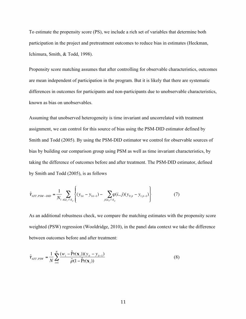
To estimate the propensity score (PS), we include a rich set of variables that determine both

participation in the project and pretreatment outcomes to reduce bias in estimates (Heckman,

Ichimura, Smith, & Todd, 1998).

Propensity score matching assumes that after controlling for observable characteristics, outcomes

are mean independent of participation in the program. But it is likely that there are systematic

differences in outcomes for participants and non-participants due to unobservable characteristics,

known as bias on unobservables.

Assuming that unobserved heterogeneity is time invariant and uncorrelated with treatment

assignment, we can control for this source of bias using the PSM-DID estimator defined by

Smith and Todd (2005). By using the PSM-DID estimator we control for observable sources of

bias by building our comparison group using PSM as well as time invariant characteristics, by

taking the difference of outcomes before and after treatment. The PSM-DID estimator, defined

by Smith and Todd (2005), is as follows

€

ˆ τ ATT ,PSM −DID =1N1

(y1it − y1it−1) − ϕ(i,, j)(y0 jt − y1 jt−1)j∈I 0 ∩Sp

∑⎫ ⎬ ⎪

⎭ ⎪

⎧ ⎨ ⎪

⎩ ⎪ i∈I1 ∩Sp

∑ (7)

As an additional robustness check, we compare the matching estimates with the propensity score

weighted (PSW) regression (Wooldridge, 2010), in the panel data context we take the difference

between outcomes before and after treatment:

€

ˆ τ ATT ,PSW =1N

(wi − ˆ P r(x i))(yit − yit−1)ˆ ρ (1− ˆ P r(x i))i=1

N

∑ (8)

  12  

For equations (8) and (9) the subscripts 1 and 0 refer to treated and untreated respectively, Sp

refers to the common support, t refers to the time period, N to the total number of observations,

ϕ(.) is a weight that depends on the matching method used, Pr(xi) is the propensity score and ρ

refers to the proportion of treated observations in the sample (N1/N).

4.2. Regression based methods.

The main assumption of FD is that the unobserved differences between participants and non-

participants are invariant in time. Examples would be particular individual characteristics like

motivation and cognitive ability. By taking the first difference we removed time invariant

unobservable characteristics. Then obtaining the first difference between periods t and t-1, the

unobservable characteristics, assumed invariant in time are eliminated, correcting for this source

of bias in the program impact estimation (Wooldridge, J., 2010):

€

Δyit = α0 +τwit + βΔx it + Δuit (9)

where Δyit=yit-yit-1, Δxit=xit-xit-1 and Δuit=uit-uit-1. We obtain the program impact by the regression

of the change in the outcome variable y the project participation variable w, and the change in a

set of time varying covariates x. The first difference equation will be consistent if E(Δxitʹ′Δuit)=0.

The parameter of interest is τ, when we omit Δxit we obtain the difference in difference (DID)

estimator.

The difference in difference estimator assumes parallel trends for both treatment and control in

the absence of the treatment (Abadie, 2005). Therefore, correcting for differences between the

two groups requires controlling for covariates related to household characteristics (Abadie,

  13  

2005). To take care of possible differences of covariates between treatment and control, we

include some time varying household characteristics as in equation (9) for estimating program

impacts.

4.3. Heterogeneity of program impacts.

Our study focuses on the ATT, the mean effect of a program on the treated. Yet as an overall

average, the ATT can miss program impacts that vary among subsets of individuals or

households. Even if our results on the program ATT for some outcomes are not statistically

significant, given the wide range of interventions within A4N, households with certain

characteristics might have benefited differentially. For example, the poorest groups might have

benefited from most of the project interventions, or to the contrary, the better off beneficiaries

might have gotten the most from the project. This analysis is conducted for different groups

identified in the sample, according to a pretreatment indicator of wealth or income generating

capacity. We estimate project impact on outcome y for each of group g.

5. Survey data use for evaluation of impacts.

The dataset was based on two-stage sampling of treatment and non-treatment villages, where

“treatment” refers to being offered the package of interventions under the A4N project. We

randomly selected villages from the list of beneficiary villages, and chose similar non-participant

villages using the population and agricultural census data from Nicaragua. The sampled villages

were selected according to the population weights of each of the municipalities where the project

intervened. Non-participant villages were identified according to national census data on poverty

  14  

levels, as measured by the index of unmet basic needs, the importance of staple crops, small

landholdings (Instituto Nacional de Información de Desarrollo, 2008a, 2008b, 2008c, 2008d,

2008e, 2008f, 2008g, 2008h), and location in the same agrarian zones (Nitlapan, 2001). From

each village we randomly selected 10 households in the participant villages and 10 to 15

households in the non-participant villages, depending on village size. In A4N participant

villages, CRS provided lists of participating households. In non-participant villages, sample lists

were developed in consultation with village leaders, who were requested to identify households

that would meet the eligibility criteria of the A4N program.

A baseline survey measured livelihoods and income for the agricultural year 2008-09, before

project implementation, and a follow up survey did the same for the agricultural year 2010-11,

the second year after project implementation. The survey also collected information on the

different technologies and practices implemented by farmers in their plots. The survey was

conducted in the departments of Estelí, Jinotega and Matagalpa, located in the northeast of

Nicaragua. The final balanced panel includes 578 households, 284 in participant villages and 294

in non-participant villages. The abandonment rate between the two rounds of the survey was 6%,

and we did found no evidence of systematic attrition. More non-participant households were

interviewed intentionally, in order to permit the trimming of observations when applying

propensity score matching. A survey of village characteristics was conducted among village

leaders in each of the 63 villages.

The data set was reduced from the original set of 578 observations due to dropping two outliers,

for a total of 576 observations. For the PSM-DID and PSW analysis, missing data for the

estimation of the PS (11 observations) and the trimming of observations with PS above 0.90 and

  15  

below 0.10 (11 observations) was conducted (Imbens & Wooldridge, 2008; Wooldridge, J.,

2010). The total number of observations used for the PSM-DID and PSW analysis is 554.

6. Results: A4N project impacts.

The estimation of project impacts starts with estimating the probability of participation in the

project using a logit model. These estimated probabilities will later be used for propensity score

matching. Balancing tests after matching are presented to measure the degree of differences

between treatment and control households. Then we show the estimated impacts for intermediate

outcomes related to the adoption of the technologies and practices promoted by the project.

Finally, we estimate project impacts by terciles of area of cultivated land.

Project treatment effects were estimated using FD, PSM-DID and PSW. The point estimates are

very similar for most of the outcomes across the methods used. We present these results showing

first the regression approach with FD and compare these results with PSM-DID and PSW in

order to compare regression-based method results with PS based methods results.

The FD estimation includes as control variables household size, average of years of education of

household members and cultivated land1. Then we estimate program impacts using PSM-DID

kernel Epanechnikov (kernel(epan)), nearest neighbor with replacement, using five neighbors

(NN(5)), and local linear regression with the tricube kernel (LLR), to conduct sensitivity analysis

of the matching results. We estimated program impact using the difference in the outcome

variables before and after the project as dependent variable, for both continuous and binary

                                                                                                               1  We also conducted fixed effects estimation, and the results did not differ from the FD ones. Therefore we consider that violation of the strict exogeneity assumption is not a concern (Wooldridge, J., 2010).  

  16  

outcomes. Treatment refers to whether the household was exposed to the package of

interventions promoted by the project2. Before presenting the results for the average treatment

effects, we present the estimation for the propensity score of probability of participating in the

A4N project.

6.1. Propensity score estimation

The probability of program participation or propensity score was estimated using a logit model

with the data from 272 treated and 282 non-treated households. Upon application of Dehejia and

Wahba’s (2002) algorithm for estimating the propensity scores, it was determined that no

interaction terms and higher level terms were justified to improve the estimation, so the logit

model was estimated with all covariates entering linearly.

The logit model estimates the probability of program participation (Table 1). Focusing on

variables that are statistically significant (p-value less than 0.10), the A4N households were more

likely to be female-headed and to have lower value of farm infrastructure but also less

inadequate services as defined by the basic needs index (housing lacking piped water and where

a toilet is missing). A4N households tended to be situated in villages closer to markets but with

fewer large farms and less likely to have a health facility. These variables reflect some

pretreatment differences between treatment and comparison households.

                                                                                                               2 Information on participation in other projects was collected in one of the household survey questions. To test for attribution to the A4N project of impacts that are due to other projects, we estimated the correlation of participation in A4N and participation in other development projects. We found no correlation (ρ=-0.03), so misattribution is not a concern. We also estimated DID including a dummy variable for participation in other projects and did not find this variable statistically significant.  

  17  

Table 1 Here

The predicted probabilities of selection into the A4N participant and non-participant groups are

presented in Figure 2. The non-participant distribution contains more observations with

propensity scores below 0.6, and a disproportionate number of observations with propensity

scores below 0.4. In spite of this, overlap does not seem to be a problem, and we have

comparison observations to match treatment ones.

Figure 2 Here

Matching of participant and non-participant observations using according to the values of the

propensity score, was conducted using STATA’s psmatch2 (Leuven & Sianesi, 2012). The

results for the balancing tests (Caliendo & Kopeinig, 2008; Wooldridge, J., 2010) after matching

with replacement are provided in Table 2. Matching improved overlap between the marginal

distributions of the covariates. As evidence, the percentage bias decreases for the covariates

below the benchmark of 25% for covariate balance (Imbens & Wooldridge, 2008).

Table 2 Here

  18  

6.2. Project impacts on outcomes related to adoption of technologies and practices.

With the goal of determining whether there was a project impact in the adoption of promoted

practices, the evaluation of intermediate outcomes focuses on six groups of outcomes: (1)

agricultural conservation structures, (2) agricultural conservation practices, (3) post-harvest grain

storage, (4) kitchen gardens, (5) saving and credit, and (6) food scarcity3. Table 3 presents

detailed definitions of the outcomes to be evaluated. Tables 4 and 5 present the results for the

average treatment effect on the treated (ATT) for the different methods use for estimating

program impacts, FD, PSM-DID for kernel(epan), NN(5) and LLR matching to compare the

sensitivity of estimates to different matching methods (Abadie & Imbens, 2008), and PSW

regression.

Table 3. Here.

The results are robust to different estimation methods, as can be seen by the similar point

estimates and levels of significance obtained for project treatment effects. Overall, our results

using FD, PSM-DID and PS weighting were almost identical. This was expected because the

sampling frame explicitly included a set of control villages and households for comparison with

similar characteristics to the A4N ones according to poverty and population indicators. The

comparison group was similar by construction to the treatment group according to observable

characteristics.

                                                                                                               3  We did not conduct impact evaluation on the use of improved maize and beans varieties due to unreliable data on the names of the varieties planted by farmers  collected in the survey.  

  19  

The construction of agricultural conservation structures and the use of agricultural conservation

practices for soil and water conservation increased thanks to the project, as shown in Table 4.

Agricultural conservation structures represent significant investments of capital and labor with a

gradual payoff. The adoption of their construction under the A4N project was measured by the

change in length of rows built structures per unit of cultivated land (meters/manzana). The

information was obtained with a recall question in 2011 on the length of agricultural

conservation structures built over the past two years. This question was asked for each of the

plots under the management of the household. On average the increase in agricultural

conservation structures was 77m/Mz, measured by first differences (Table 4); the estimates for

PSM-DID and PSW are similar, and all are highly statistically significant. This increase was

explained mostly by the increase in area under stone barriers and terraces (24m/Mz), live barriers

(16m/Mz), and ditches (7m/Mz) (Table 4).

Table 4. Here

Agricultural conservation practices included reduced tillage, vermiculture and cover crops, all

three of which are much less demanding than the construction of terraces, barriers, or ditches.

The adoption of practices was measured by changes in whether the household was implementing

one or more of the practices promoted by A4N on at least one of the plots managed by the

household. On average there was not an overall impact in the use of these practices, but there

was significant substitution of minimum tillage for zero tillage. The percentage of households

using minimum tillage in at least one of their plots decreased by 14%, whereas this percentage

  20  

increased by 19% for zero tillage (Table 4). In addition, there was an increase in households

implementing vermiculture and cover crops in at least one of their plots.

The project had a significant, positive effect on adoption of metallic silos for grain storage. On

average there was an increase of 11% in the share of households using metallic silos for storage

(Table 5). Presumably associated with this, the number of households that experienced stored

grain losses fell by 11% to 16%, based the four estimates with p-values below 0.15. The

increased use of metallic silos translated into a reduction on stored grain losses within the first

two years of the A4N project, and it is possible that project beneficiaries were still in the process

of learning how to best apply postharvest management practices to avoid losses. The successful

adoption of these practice can lead to further reduction of losses of grain stored for consumption

(Gitonga, De Groote, Kassie, & Tefera, 2013).

Table 5. Here

The project had a significant impact in the percentage of households with savings, which

increased by 14% (Table 5). This is not an agricultural technology intervention, but this was a

very successful intervention of the project that aimed to stabilize income flow over the year and

to provide funds in times of household food scarcity. This outcome is mostly a result of the

formation of saving and lending groups promoted by the project. Savings gains are likely to

reduce vulnerability to asset liquidation in times of food scarcity, and consumption smoothing

(Kaboski & Townsend, 2005). Savings accumulation can also be used for productive investments

(e.g., in agricultural assets) (Chowa & Elliott III, 2011).

  21  

6.3. Heterogeneity if project impacts by area of cultivated land.

Continuing with the analysis of project impacts, we look at the distribution of project effects

across households of varying asset levels. It is possible that even if average treatment effects for

the agricultural income and household wealth related outcomes were not statistically significant,

some groups benefited more (or less) than others (Khandker, Koolwal, & Samad, 2010). The

sample was divided into approximate terciles using the information on the pretreatment area of

cultivated land. Farmland, an important asset, is the key input for agricultural production. The

first group is composed of households with less than 1.5 Mz (small area) of cultivated land, the

second one with households with between 1.5 Mz and 3 Mz of land (medium area) and the third

one with households with more than 3 Mz of cultivated land (large area).

Table 6 presents the estimated coefficients of average treatment effects for each of the three

groups formed using the area of cultivated land in 2009. The FD, PSM-DID and PSW estimates

of average treatment effects are all very similar, so for this analysis we simply report FD, for

each tercile of area of cultivated land. The FD estimation uses the same explanatory variables as

those included in the estimation of overall program effects: household size, average of years of

education of household members and cultivated land.

Table 6. Here.

The results pointed to notable differences in impact by asset level. Households with large and

medium area of cultivated land built higher densities of agricultural conservation structures,

  22  

whereas households with small area were more likely to increase their use of agricultural

conservation practices. On average, households with medium and large cultivated area built

41m/Mz and 74m/Mz of agricultural conservation structures (see Table 6). The implementation

of agricultural conservation practices in at least one of the plots under the management of the

household increased by 20% among the households with small area, and 20% of these

households also increased the use of zero tillage. In contrast, 30% of households with larger area

decreased their use of minimum tillage, and 19% increased the use of zero tillage (Table 6).

These results are consistent with results of studies about decisions of carrying out agricultural

conservation investments, which depend on access to land and labor, as well as land tenure

security (Gebremedhin & Swinton, 2003), indicating that differences in household characteristics

matter for household decisions of take up of project interventions.

The households with medium cultivated area are the ones most likely to increase adoption of

improved grain storage practices and to experience decreased stored grain losses. A total of 30%

more of medium area households experienced reduced losses of stored grain, and 16% more of

these households stored grain in metallic silos (Table 6).

Households with small cultivated area were the ones to add kitchen gardens and to gain savings.

The ATT for households with kitchen gardens was not statistically significant for the whole

sample, but 12% more households with small land area have kitchen gardens thanks to the

project (Table 6), which in turn helps to improve food security. Also these households are the

ones that take advantage of the creation of savings and lending groups, with a 22% increase in

households with savings.

  23  

These results suggest that household resource constraints may limit adoption of certain practices.

Capital is required to undertake the investments in construction of agricultural structures,

including the hiring of labor. For households with small cultivated area, practices that do not

require this level of investment, such as participation in savings groups or growing small

vegetable gardens, constitute practices that they are more likely to adopt.

7. Conclusion

Using different methods, FD, PSM-DID and PSW, we find identical results. Stability of project

impact estimates across the methods used was expected. Due to careful design of the impact

evaluation with data collected of comparison households to construct a valid counterfactual for

analysis.

We focused on the adoption of improved agricultural technologies to measure changes in

behavior, as early indicators of project impact. We found that adoption did increase for many of

the technologies promoted. If these behavioral changes are maintained over time, they are likely

to translate into increases in agricultural productivity and agricultural income by several

mechanisms: Investments in agricultural conservation structures and adoption of agricultural

conservation practices are both likely to lead to long-term stabilization of yields. Adoption of

improved storage technologies, the associated reduction in the number of households

experiencing stored grain losses, and increases in households with savings should all lead to

more stable, rising cash flows and reduced of risks of food scarcity and asset liquidation.

However, rates of adoption of project technologies were not the same across households of

different asset levels. The analysis of project impacts by farm size reveals that they vary

  24  

according to the household’s area of cultivated land. Hence, the targeting of project

interventions by participant asset level can increase rates of adoption of practices by tailoring

interventions to household resources. Such an approach could increase project impacts for

different groups of beneficiaries, instead of promoting all the interventions for all the

beneficiaries—a more cost-effective strategy.

An important recommendation from this impact assessment is that the heterogeneity across

project interventions of the expected time lapse before participants experience benefits should be

considered both for project design and for impact evaluation. As shown here, the realization of

gains for some interventions (e.g. construction of stone barriers and terraces) takes much longer

than others (e.g. storage in metallic silos). Therefore, development projects that promote multiple

interventions may want to set poverty relief objectives that explicitly incorporate the timing of

expected benefits from adoption of specific practices. In an environment of donor impatience to

see rapid impacts, such an approach would calibrate donor expectations to a realistic sequence of

intermediate impacts that culminate in long-term desired outcomes.

  25  

Figure 1. Impact trajectories of different type of project interventions.

Adapted from King and Behrman (2009)

Impact

Impact

time

time

t1

t1

I

II

 

  26  

Figure  1. Estimated propensity score or probability of program participation.

  27  

Table 1. Logit model for estimating the propensity score or probability of participation in A4N.

 

Explanatory variables Coefficient Standard

errors Farm characteristics Cultivated land Mz 0.03 (0.03) Steep slope=1 0.18 (0.20) hh characteristics Inadequate services=1 -0.51** (0.22) Inadequate housing=1 0.11 (0.29) Electricity=1 -0.05 (0.22) Hunger=1 0.34* (0.20) head female=1 1.19*** (0.31) #children<5 0.06 (0.15) head age 0.00 (0.01) head education -0.01 (0.04) household size -0.05 (0.06) people per room -0.02 (0.06) Value of productive assets Infraestructure C$/1000 -0.09* (0.06) Livestock C$/1000 -0.02* (0.01) Equipment C$/1000 0.00 (0.02) Village charcteristics Population 2009 0.00 (0.00) Dist. Market Km/10 -0.05*** (0.01) Dist. Paved road Km/10 0.02 (0.01) Health facility=1 -0.82*** (0.26) % basic grains 2003 -0.18 (0.63) % lanholdings<10Mz 2003 2.25*** (0.50) Constant -0.20 (0.84) Log likelihood -345 n 554 Levels of significance ***1%, **5%, *10% Standard error in parenthesis 1 Mz = 1.73 acres U$1=C$22.42 in 2011

  28  

Table 2. Balancing tests of pretreatment covariates used for estimation of the propensity score.

Before matching After matching Mean Mean

Variable A4N Non-A4N %bias A4N

Non-A4N %bias

Cultivated land Mz 3.29 3.50 -2.68 3.32 3.37 -1.6 Steep slope=1 0.32 0.32 -25.87 0.32 0.37 -9.7 Inadequate services=1 0.66 0.79 21.39 0.67 0.66 3.6 Inadequate housing=1 0.88 0.85 60.10 0.88 0.86 4.4 Electricity=1 0.61 0.63 15.32 0.60 0.58 4.9 Hunger=1 0.39 0.32 -17.89 0.38 0.40 -4.2 head female=1 0.20 0.07 -73.06 0.18 0.22 -12.8 #children<5 0.51 0.51 -24.23 0.51 0.41 14.1 head age 49 48 68 49 49 -1.2 head education 2.83 3.04 3.13 2.84 2.79 1.7 household size 5.20 5.36 49.55 5.20 4.99 9.3 people per room 3.82 3.86 40.94 3.84 3.85 -0.6 Infraestructure C$/1000 0.52 1.48 -11.12 0.53 0.47 3.3 Livestock C$/1000 6.71 9.07 -17.33 6.80 6.08 5.7 Equipment C$/1000 1.76 2.08 -49.91 1.80 2.09 -6.2 Population 2009 637 640 16.68 645 678 -5.9 Dist. Market Km/10 14.09 16.29 38.19 14.34 14.46 -1.5 Dist. Paved road Km/10 9.53 8.95 -0.99 9.56 8.63 10 Health facility=1 0.21 0.28 -37.29 0.21 0.21 0.7 % basic grains 2003 0.86 0.88 71.93 0.86 0.87 -4.9 % lanholdings<10Mz 2003 0.59 0.52 64.34 0.58 0.54 18

1 Mz = 1.73 Acres U$1=C$22.42

  29  

Table 3. Definition of intermediate outcome variables and units of measurement.

Outcome Variables Unit Definition Agricultural Conservation Structures (Length built in meters between 2009 and 2011)

All structures m/Mz

Difference length built in agricultural conservation structures 2011-2009

Stone barriers/terraces m/Mz

Difference length built in stone barriers and terraces 2011-2009

Live barriers m/Mz Difference length built in live barriers 2011-2009 Ditches m/Mz Difference length built in ditches 2011-2009 Agricultural Conservation Practices

All practices 1=yes, 0=no

The household has implemented at least one cons ag practice in one of the plots under its management

Minimum tillage 1=yes, 0=no

The household has implemented minimum tillage at least in one plot

Zero tillage 1=yes, 0=no

The household has implemented zero tillage at least in one of its plots

Vermiculture 1=yes, 0=no

The household has implemented vermiculture at least in one of its plots

Cover crops 1=yes, 0=no

The household has implemented cover crops at leas in one of its plots

Storage Practices Household experienced stored grain losses 1=yes, 0=no

The household has experienced stored grain losses. Only for households that stored grain.

Household stored grain in metallic silos 1=yes, 0=no

The household uses metallic silos for grain storage. Only for households that stored grain

Number of metallic silos number Number of metallic silos owned by the household Kitchen Garden hh had a kitchen garden 1=yes, 0=no Household has a kitchen garden Savings and Credit hh has savings 1=yes, 0=no Household had savings on January 1st hh has credit 1=yes, 0=no Household had credit on January 1st Food Scarcity hh experience food scarcity 1=yes, 0=no

Household experienced a period of the year when they could not cook one of the daily meals

hh means household 1 Mz = 1.73 acres

  30  

Table 4.  Project impacts on construction of agricultural conservation structures and on agricultural conservation practices.  

PSM-DID

Difference outcome variables FD

kernel (epan) NN(5)

llr (tricube) PSW

Agricultural Conservation Structures 77*** 76*** 75*** 73*** 72*** All structures

m/Mz (25) (25) (27) (27) (27) 24*** 24*** 23** 22** 24** Stone

barriers/terraces m/Mz

(10) (10) (10) (11) (10)

16*** 17*** 17*** 17*** 17*** Live barriers m/Mz (5) (5) (6) (5) (5) Ditches m/Mz 7*** 7*** 8*** 7*** 7*** (3) (3) (3) (3) (3)

Agricultural Conservation Practices 0.04 -0.02 -0.03 -0.02 0.00 All practices1

(0.05) (0.06) (0.06) (0.06) (0.05) -0.14*** -0.17*** -0.16** -0.17** -0.15*** Minimum tillage1

(0.05) (0.07) (0.08) (0.07) (0.05) 0.19*** 0.19*** 0.20*** 0.18*** 0.18*** Zero tillage1

(0.0 (0.07) (0.07) (0.07) (0.07) 0.05*** 0.05** 0.05** 0.05** 0.04*** Vermiculture1 (0.02) (0.02) (0.02) (0.02) (0.02)

0.03*** 0.04* 0.04* 0.04* 0.04* Cover crops1 (0.01) (0.02) (0.02) (0.02) (0.02)

Levels of significance ***1%, **5%, *10% NN refers to nearest neighbor, LLR to local linear regression untrimmed sample n=567, trimmed sample n=546 A total of 265 pairs formed with PSM-DID 1 Mz = 1.73 acres 1 For binary outcomes the difference takes values -1, 0 and 1.

  31  

Table 5.  Project impacts on storage practices, kitchen gardens, savings and credit and food scarcity.  

PSM-DID Difference outcome variables FD

kernel (epan) NN(5)

llr (tricube) PSW

Storage Practices -0.16*** -0.11~ -0.07 -0.13~ -0.11~ Experienced

stored grain losses1,2

(0.06) (0.08) (0.08) (0.09) (0.08)

0.11*** 0.10** 0.11** 0.10* 0.09~ hh stored grain in metalic silos1,2 (0.04) (0.05) (0.05) (0.05) (0.06)

0.14*** 0.13*** 0.12** 0.13*** 0.13*** Number of metalic silos owned

(0.05) (0.05) (0.06) (0.05) (0.05)

Kitchen garden 0.04 0.04 0.04 0.04 0.04 hh had a kitchen

garden1 (0.03) (0.04) (0.03) (0.03) (0.03) Savings and credit

0.14*** 0.13*** 0.13*** 0.12*** 0.13*** hh has savings1 (0.04) (0.04) (0.05) (0.05) (0.04) -0.01 -0.01 -0.03 -0.03 0.00 hh has credit1 (0.04) (0.05) (0.06) (0.05) (0.05)

Food scarcity -0.06 0.04 0.05 0.05 0.04 hh experienced

food scarcity1 (0.05) (0.05) (0.06) (0.05) (0.04) 2 Correspond only to the households that stored grain, non trimmed sample n=476, trimmed sample n=460 1 For binary outcomes the difference takes values -1, 0 and 1 Levels of significance ***1%, **5%, *10%, ~ 15%. NN refers to nearest neighbor, LLR to local linear regression hh means household untrimmed sample n=575, trimmed sample n=554 A total of 265 pairs formed with PSM-DID

  32  

 

Table 6. Project impacts by area of cultivated land on outcomes related to adoption of practices and technologies.  

<=1.5Mz

n=191 1.5<land<=3Mz

n=199 >3Mz n=186

Outcomes Coef se Coef se Coef se Agricultural Conservation structures All structures m/Mz 111 (73) 41*** (16) 74*** (27) Stone barriers m/Mz 3 (27) 27** (12) 31*** (11) Live barriers m/Mz 16 (15) 13*** (5) 18*** (7) Ditches m/Mz 11** (5) 4** (2) 8 (8) Agricultural conservation practices All practices1 0.20** (0.09) -0.03 (0.08) -0.06 (0.06) Minimum tillage1 -0.08 (0.09) -0.05 (0.09) -0.30** (0.09) Zero tillage1 0.20** (0.08) 0.15 (0.08) 0.19* (0.08) Vermiculture1 0.05** (0.03) 0.02 (0.02) 0.08* (0.04) Cover crops1 0.03 (0.02) 0.02 (0.02) 0.03 (0.02) Storage Practices Stored grain losses1 -0.06 (0.12) -0.28*** (0.09) -0.12 (0.09) Stored in metallic silos1 0.06 (0.06) 0.15** (0.06) 0.10 (0.08) Number of metallic silos owned 0.07 (0.07) 0.16** (0.07) 0.21* (0.10) Kitchen garden hh has a kitchen garden1 0.12** (0.05) -0.02 (0.04) 0.02 (0.05) Saving and credit Saving1 0.22*** (0.07) 0.08 (0.06) 0.09 (0.08) Credit1 0.10 (0.07) -0.03 (0.07) -0.13 (0.09) Food scarcity Experienced period of hunger1 -0.03 (0.08) -0.06 (0.08) -0.08 (0.08)

1 For binary outcomes the difference takes values -1, 0 and 1 1 Mz = 1.73 acres hh means household Note: the total sample of 576 observations was divided in terciles, and for each tercile there was an approximate equal share of treatment and comparison observations.

  33  

 

References

Abadie, A. (2005). Semiparametric Difference-in-Differences Estimators. The Review of

Economic Studies, 72(1), 1–19. doi:10.1111/0034-6527.00321

Abadie, A., & Imbens, G. W. (2008). On the Failure of the Bootstrap for Matching Estimators.

Econometrica, 76(6), 1537–1557. doi:10.3982/ECTA6474

Besley, T., & Case, A. (1993). Modeling Technology Adoption in Developing Countries. The

American Economic Review, 83(2), 396–402. doi:10.2307/2117697

Byerlee, D., & Hesse de Polanco, E. (1986). Farmers’ Stepwise Adoption of Technological

Packages: Evidence from the Mexican Altiplano. American Journal of Agricultural

Economics, 68(3), 519–527. doi:10.2307/1241537

Caliendo, M., & Kopeinig, S. (2008). Some practical guidance for the implementation of

propensity score matching. Journal of economic surveys, 22(1), 31–72.

Chowa, G. A. N., & Elliott III, W. (2011). An asset approach to increasing perceived household

economic stability among families in Uganda. The Journal of Socio-Economics, 40(1),

81–87. doi:10.1016/j.socec.2010.02.008

Cuong, N. V. (2009). Impact evaluation of multiple overlapping programs under a conditional

independence assumption. Research in Economics, 63(1), 27–54.

doi:10.1016/j.rie.2008.10.001

Dehejia, R. H., & Wahba, S. (2002). Propensity score-matching methods for nonexperimental

causal studies. Review of Economics and statistics, 84(1), 151–161.

  34  

Feder, G., Just, R. E., & Zilberman, D. (1985). Adoption of Agricultural Innovations in

Developing Countries: A Survey. Economic Development and Cultural Change, 33(2),

255–298. doi:10.2307/1153228

Gebremedhin, B., & Swinton, S. M. (2003). Investment in soil conservation in northern Ethiopia:

the role of land tenure security and public programs. Agricultural Economics, 29(1), 69–

84. doi:10.1111/j.1574-0862.2003.tb00148.x

Gitonga, Z. M., De Groote, H., Kassie, M., & Tefera, T. (2013). Impact of metal silos on

households’ maize storage, storage losses and food security: An application of a

propensity score matching. Food Policy, 43, 44–55. doi:10.1016/j.foodpol.2013.08.005

Heckman, J.J., Ichimura, H., Smith, J., & Todd, P. (1998). Characterizing Selection Bias Using

Experimental Data. Econometrica, 66(5), 1017–1098. doi:10.2307/2999630

Heckman, James J., Ichimura, H., & Todd, P. E. (1997). Matching As An Econometric

Evaluation Estimator: Evidence from Evaluating a Job Training Programme. The Review

of Economic Studies, 64(4), 605–654. doi:10.2307/2971733

Imbens, G. M., & Wooldridge, J. M. (2008). Recent developments in the econometrics of

program evaluation. National Bureau of Economic Research. Retrieved from

http://www.nber.org/papers/w14251

Instituto Nacional de Información de Desarrollo. (2008a). Esquipulas en cifras. Instituto

Nacional de Informacion de Desarrollo. Retrieved from

http://www.inide.gob.ni/censos2005/CifrasMun/tablas_cifras.htm

Instituto Nacional de Información de Desarrollo. (2008b). Esteli en cifras. Instituto Nacional de

Informacion de Desarrollo. Retrieved from

http://www.inide.gob.ni/censos2005/CifrasMun/tablas_cifras.htm

  35  

Instituto Nacional de Información de Desarrollo. (2008c). Jinotega en cifras. Instituto Nacional

de Informacion de Desarrollo. Retrieved from

http://www.inide.gob.ni/censos2005/CifrasMun/tablas_cifras.htm

Instituto Nacional de Información de Desarrollo. (2008d). La Trinidad en cifras. Instituto

Nacional de Informacion de Desarrollo. Retrieved from

http://www.inide.gob.ni/censos2005/CifrasMun/tablas_cifras.htm

Instituto Nacional de Información de Desarrollo. (2008e). San Isidro en cifras. Instituto Nacional

de Informacion de Desarrollo. Retrieved from

http://www.inide.gob.ni/censos2005/CifrasMun/tablas_cifras.htm

Instituto Nacional de Información de Desarrollo. (2008f). San Nicolas en cifras. Instituto

Nacional de Informacion de Desarrollo. Retrieved from

http://www.inide.gob.ni/censos2005/CifrasMun/tablas_cifras.htm

Instituto Nacional de Información de Desarrollo. (2008g). San Rafael del Norte en cifras.

Instituto Nacional de Informacion de Desarrollo. Retrieved from

http://www.inide.gob.ni/censos2005/CifrasMun/tablas_cifras.htm

Instituto Nacional de Información de Desarrollo. (2008h). Terrabona en cifras. Instituto Nacional

de Informacion de Desarrollo. Retrieved from

http://www.inide.gob.ni/censos2005/CifrasMun/tablas_cifras.htm

International Fund for Agricultural Development. (2010). Rural Poverty Report 2011. New

realities, new challenges: new opportunities for tomorrow’s generation. International

Fund for Agricultural Development (IFAD).

  36  

Kaboski, J. P., & Townsend, R. M. (2005). Policies and Impact: An Analysis of Village-Level

Microfinance Institutions. Journal of the European Economic Association, 3(1), 1–50.

doi:10.1162/1542476053295331

Khandker, S. R., Koolwal, G. B., & Samad, H. A. (2010). Handbook on Impact Evaluation:

Quantitative Methods and Practices. World Bank Publications.

King, E. M., & Behrman, J. R. (2009). Timing and Duration of Exposure in Evaluations of

Social Programs. The World Bank Research Observer, 24(1), 55–82.

doi:10.1093/wbro/lkn009

Lechner, M. (2001). Identification and estimation of causal effects of multiple treatments under

the conditional independence assumption. Econometric evaluation of labour market

policies, 43–58.

Leuven, E., & Sianesi, B. (2012). PSMATCH2: Stata module to perform full Mahalanobis and

propensity score matching, common support graphing, and covariate imbalance test.

Nitlapan. (2001). Tipología Nacional de Productores y Zonificación Socio-económica. Managua:

Nitlapan.

Nowak, P. (1992). Why farmers adopt production technology Overcoming impediments to

adoption of crop residue management techniques will be crucial to implementation of

conservation compliance plans. Journal of Soil and Water Conservation, 47(1), 14–16.

Ravallion, M. (2008). Evaluation in the Practice of Development (SSRN Scholarly Paper No. ID

1103727). Rochester, NY: Social Science Research Network. Retrieved from

http://papers.ssrn.com/abstract=1103727

Smith, J., & Todd, P. (2005). Does matching overcome LaLonde’s critique of nonexperimental

estimators? Journal of econometrics, 125(1), 305–353.

  37  

Sunding, D., & Zilberman, D. (2001). Chapter 4 The agricultural innovation process: Research

and technology adoption in a changing agricultural sector. In Bruce L. Gardner and

Gordon C. Rausser (Ed.), Handbook of Agricultural Economics (Vol. Volume 1, Part A,

pp. 207–261). Elsevier. Retrieved from

http://www.sciencedirect.com/science/article/pii/S1574007201100071

Teklewold, H., Kassie, M., & Shiferaw, B. (2013). Adoption of Multiple Sustainable

Agricultural Practices in Rural Ethiopia. Journal of Agricultural Economics, 64(3), 597–

623. doi:10.1111/1477-9552.12011

Tjernström, E., Toledo, P., & Carter, M. R. (2013). Identifying the Impact Dynamics of a Small-

Farmer Development Scheme in Nicaragua. American Journal of Agricultural

Economics, 95(5), 1359–1365. doi:10.1093/ajae/aat042

Wooldridge, J. (2010). Econometric Analysis of Cross Section and Panel Data. Cambridge,

Massachusetts: The MIT Press.

World Bank. (2008). Poverty Assessment Nicaragua (No. 39736-NI) (p. 215). Retrieved from

http://web.worldbank.org/WBSITE/EXTERNAL/TOPICS/EXTPOVERTY/EXTPA/0,,co

ntentMDK:20207612~menuPK:435735~pagePK:148956~piPK:216618~theSitePK:4303

67~isCURL:Y~isCURL:Y,00.html