impact 2002+: user guide - quantis | sustainability ...€¦ · 1 life cycle assessment expert,...
TRANSCRIPT

IMPACT2002+_UserGuide_for_vQ2 21_1November2012
i
IMPACT 2002+: User Guide
Draft for version Q2.21
(version adapted by Quantis)
Prepared by:
Sébastien Humbert1*
An De Schryver1
Xavier Bengoa1
Manuele Margni2
Olivier Jolliet3
* Corresponding author ([email protected],
1
Life Cycle Assessment Expert, Quantis, Lausanne, Switzerland 2
CIRAIG, École Polytechnique de Montréal, Montréal QC, Canada 3
Center for Risk Science and Communication, Department of Environmental Health
Sciences, School of Public Health, University of Michigan, Ann Arbor MI, USA
IMPACT 2002+ is a methodology that was originally developed at the Swiss Federal
Institute of Technology Lausanne (EPFL), Switzerland. It is now maintained and further
developed by The IMPACT Modeling Team.
November 1, 2012
Note:
The difference between the versions Q2.21 (November 2012) and 2.2 (March 2012) is an additional set of characterization factors improving the method’s
completeness. All changes are documented in the Annex 5.
The difference between the versions Q2.2 (updated by Quantis) and 2.1 are mainly that water turbined, water withdrawal and water consumption are
added, and that aquatic acidification, aquatic eutrophication and water turbined are brought to the damage category ecosystem quality. Furthermore,
climate change CFs are adapted with GWP for 100 year time horizon.
The differences between the versions v2.1 and v2.0 are minor. They concern mainly 1° adaptation reflecting the update of the DALY used per case of cancer
and non-cancer (respectively 13 and 1.3 instead of 6.7 and 0.67) and 2° some format update (typos corrected, email addresses updated, font improved,
references updated, etc.).

IMPACT2002+_UserGuide_for_vQ2 21_1November2012
ii
A user guide for the Life Cycle Impact Assessment Methodology
IMPACT 2002+ (Jolliet et al. 2003c)
The paper (Jolliet et al. 2003c) and characterization factors
(IMPACT2002+_vQ2.2_CF_1a.xls) can be downloaded at
http://www.quantis-intl.com
The supporting paper (Jolliet et al. 2003c) and (Pennington et al. 2005) can be
obtained via the International Journal of Life Cycle Assessment
(http://www.scientificjournals.com/sj/lca/Pdf/aId/6237 or
http://dx.doi.org/10.1007/BF02978505) and the Environmental Science and
Technology (http://pubs.acs.org/journals/esthag/) websites respectively.
This user guide is intended for supporting users to apply and interpret the
LCIA methodology IMPACT 2002+ version Q2.21.

IMPACT2002+_UserGuide_for_vQ2 21_1November2012
iii
Why a version adapted by Quantis and what has been adapted?
The original IMPACT 2002+ version 2.1 is not bringing all possible impact categories to an
endpoint and neglects some impact categories which are increasingly demanded by industry. We see
it necessary to create an adapted version Q2.2 for the following reasons:
1. There is a strong demand of companies for analyzing climate change using IPCC 100 year
instead of 500 year time horizon
2. Issues relating to water withdrawal, consumption and turbine are increasingly demanded by
companies and should be considered
3. Eutrophication and acidification should be brought to endpoint level to add capacity to
interpret results of ecosystem quality at endpoint without neglecting these important
categories
The following adaptations are made in vQ2.2 (March 2012) and vQ2.21 (November 2012):
1. Climate change CFs are adapted a 100 year time horizon
2. Water withdrawal, water consumption and water turbined are added
3. Aquatic acidification, aquatic eutrophication and water turbined are added at endpoint to the
damage category ecosystem quality
4. Normalization factors are updated
5. (November 2012) New set of characterization factors (see Annex 5 for details)

IMPACT2002+_UserGuide_for_vQ2 21_1November2012
iv
CONTENT
ABSTRACT ......................................................................................................................... 1
KEYWORDS ....................................................................................................................... 1
0. INTRODUCTION ....................................................................................................... 2
0.1. STRUCTURE OF LCA ............................................................................................... 2 0.2. PRINCIPLES OF LCIA .............................................................................................. 2
1. IMPACT 2002+: GENERAL CONCEPT ................................................................. 3
1.1. IMPACT 2002+: GENERAL CHARACTERISTICS ....................................................... 4
1.2. UNITS ..................................................................................................................... 5 1.3. MIDPOINT CATEGORIES........................................................................................... 7
1.3.1. Human toxicity (carcinogenic and non-carcinogenic effects) ....................... 7
1.3.2. Respiratory effects (caused by inorganics) ................................................... 8 1.3.3. Ionizing radiation .......................................................................................... 9 1.3.4. Ozone layer depletion .................................................................................... 9 1.3.5. Photochemical oxidation ............................................................................... 9
1.3.6. Aquatic ecotoxicity ........................................................................................ 9 1.3.7. Terrestrial ecotoxicity .................................................................................. 10
1.3.8. Aquatic acidification .................................................................................... 10 1.3.9. Aquatic eutrophication ................................................................................ 10 1.3.10. Terrestrial acidification & nutrification ...................................................... 11
1.3.11. Land occupation .......................................................................................... 11 1.3.12. Water turbined ............................................................................................. 11
1.3.13. Global warming ........................................................................................... 12 1.3.14. Non-renewable energy ................................................................................. 13 1.3.15. Mineral extraction ....................................................................................... 13
1.3.16. Water withdrawal ........................................................................................ 14
1.3.17. Water consumption ...................................................................................... 14 1.4. DAMAGE CATEGORIES .......................................................................................... 14
1.4.1. Human health .............................................................................................. 15 1.4.2. Ecosystem quality ........................................................................................ 15 1.4.2.1. Transformation of units ............................................................................... 15
1.4.3. Climate change ............................................................................................ 16 1.4.4. Resources ..................................................................................................... 16
1.5. NORMALIZATION .................................................................................................. 16
2. CAUTIONS, LIMITATIONS AND INTERPRETATION ................................... 18
2.1. LINK BETWEEN LIFE CYCLE INVENTORY AND LIFE CYCLE IMPACT ASSESSMENT 18 2.1.1. Some relevant points to be aware of ............................................................ 18 2.1.2. Implementation in different types of software ............................................. 18
2.2. HOW TO CHECK AND INTERPRET RESULTS? ........................................................... 18 2.3. UNCERTAINTIES .................................................................................................... 20
3. WEIGHTING ............................................................................................................. 21
4. ABBREVIATIONS AND NUMERICAL HYPOTHESIS ..................................... 22
4.1. ABBREVIATIONS AND GLOSSARY ......................................................................... 22 4.2. NUMERICAL HYPOTHESIS ..................................................................................... 23

IMPACT2002+_UserGuide_for_vQ2 21_1November2012
v
5. ACKNOWLEDGEMENTS ...................................................................................... 24
6. SOURCES .................................................................................................................. 24
6.1. REFERENCES ......................................................................................................... 24 6.2. INTERNET LINKS AND DOWNLOADABLE FILES ...................................................... 27
7. ANNEXES .................................................................................................................. 29
7.1. ANNEX 1: NORMALIZATION FACTORS FOR THE MIDPOINT CATEGORIES ................ 29 7.2. ANNEX 2: THE MIXING TRIANGLE ......................................................................... 30
7.3. ANNEX 3: HOW TO USE IMPACT 2002+ IN DIFFERENT SOFTWARE? .................... 31 7.4. ANNEX 4: HISTORICAL CHANGES OF IMPACT 2002+ .......................................... 32 7.5. ANNEX 5: IMPACT 2002+ VQ2.21 ADDED SUBSTANCES ..................................... 33

IMPACT2002+_UserGuide_for_vQ2 21_1November2012
1
Abstract The life cycle impact assessment methodology IMPACT 2002+ vQ2.2 (version adapted by Quantis)
proposes a feasible implementation of a combined midpoint/damage approach, linking all types of life
cycle inventory results (elementary flows and other interventions) via several midpoint categories to
several damage categories. For IMPACT 2002+ vQ2.2 new concepts and methods have been developed,
especially for the comparative assessment of human toxicity and ecotoxicity as well as inclusion of impacts
from turbined water and assessment of water withdrawal and consumption. IMPACT 2002+ vQ2.2 considers
several midpoint categories, namely human toxicity carcinogenic effects, human toxicity non-carcinogenic
effects (these two categories are sometimes grouped in one category: human toxicity), respiratory effects
(due to inorganics), ionizing radiation, ozone layer depletion, photochemical oxidation, aquatic ecotoxicity,
terrestrial ecotoxicity, aquatic acidification, aquatic eutrophication, terrestrial acidification/nutrification1, land
occupation, water turbined, global warming, non-renewable energy consumption, mineral extraction, water
withdrawal and water consumption. All midpoint scores are expressed in units of a reference substance and
related to the four damage categories human health, ecosystem quality, climate change, and resources. These
four damage categories are expressed respectively in DALY, PDF·m2·y, kg CO2-eq, and MJ. Normalization
can be performed either at midpoint or at damage level. The IMPACT 2002+ methodology presently
provides midpoint characterization factors, damage factors, normalized midpoint characterization factors and
normalized damage factors for almost 1500 different life cycle inventory results, which can be downloaded at
http://www.impactmodeling.org (IMPACT 2002+ v2.1) or http://www.quantis-intl.com (IMPACT 2002+
vQ2.2, version adapted by Quantis, presented in the current document).
Keywords IMPACT 2002+; life cycle assessment; life cycle impact assessment; midpoint/damage approach;
characterization/damage/normalization factors; human toxicity; carcinogenic; non-carcinogenic; respiratory
effects; ionizing radiation; ozone layer depletion; photochemical oxidation; aquatic ecotoxicity; terrestrial
ecotoxicity; aquatic acidification; aquatic eutrophication; terrestrial acidification/nutrification; land
occupation; water turbined; global warming; non-renewable energy consumption; mineral extraction; water
withdrawal; water consumption; human health; ecosystem quality; climate change; resources.
1 Note that some documents use the term “nitrification” instead of “nutrification”. Because the method Eco-indicator 99 uses the term
“nutrification” we decided to use the same for simplification reasons.

IMPACT2002+_UserGuide_for_vQ2 21_1November2012
2
0. Introduction
0.1. Structure of LCA
According to ISO 14044 life cycle assessment (LCA) is a method for assessing the environmental aspects
and potential impacts associated with a good or a service delivered, by:
compiling an inventory of relevant input and output of a product system [i.e., the life cycle
inventory (LCI)],
evaluating the potential environmental impacts associated with those inputs and outputs [i.e., the life
cycle impact assessment (LCIA)] through the use of characterization factors (CFs), and
interpreting the results of the inventory analysis and impacts assessment phases in relation to the
objective of the study.
0.2. Principles of LCIA
According to ISO 14040 and ISO 14044, life cycle assessment (LCA) is a method for assessing the
environmental aspects and potential impacts associated with a good or a service delivered by the following:
identify product system improvement opportunities and assist the prioritization of them,
characterize or benchmark a product system and its unit processes over time,
make relative comparisons among product systems based on selected category indicators, or
indicate environmental issues for which other techniques can provide complementary environmental
data and information useful to decision-makers.
Thus LCIA methodologies aim to connect, as far as possible and desired, each LCI result (elementary flow or
other intervention) to the corresponding environmental impacts by using CFs. According to ISO 14044, LCI
results are classified into impact categories, each with a category indicator. The category indicator can be
located at any point between the LCI results and the damage category (where the environmental effect
occurs) in the cause-effect chain. Within this framework, two main schools of methodologies have evolved:
a) Classical impact assessment methodologies [e.g., CML (Guinée et al. 2002) and EDIP (Hauschild
and Wenzel 1998)] restrict quantitative modeling to relatively early stages in the cause-effect chain
and, classify and characterize LCI results in so-called midpoint categories by quantifying midpoint
CFs. Themes are common mechanisms (e.g., climate change) or commonly accepted grouping (e.g.,
aquatic ecotoxicity).
b) Damage oriented methodologies such as ReCiPe (Goedkoop et al. 2008), Eco-indicator 99
(Goedkoop and Spriensma 2000) or EPS (Steen 1999) try to model the cause-effect chain up to the
damage and quantify endpoint CFs.
The definition study of the UNEP-SETAC Life Cycle Initiative suggests utilizing the advantages of both
approaches by grouping similar category endpoints into a structured set of damage categories. In addition, the
concept also works with midpoint categories, each midpoint category relating to one or several damage
categories. IMPACT 2002+ addresses this new challenge by presenting an implementation working both at
midpoint and damage.

IMPACT2002+_UserGuide_for_vQ2 21_1November2012
3
1. IMPACT 2002+: general concept
Figure 1-1: Overall scheme of the IMPACT 2002+ vQ2.2 framework2, linking LCI results via the
midpoint categories to damage categories, based on Jolliet et al. (2003a).
As shown in Figure 1-1, LCI results with similar impact pathways (e.g., all elementary flows influencing the
stratospheric ozone concentration) are allocated to impact categories at midpoint level, also called midpoint
categories. A midpoint indicator characterizes the elementary flows and other environmental interventions
that contribute to the same impact. The term ‘midpoint’ expresses the fact that this point is located
somewhere on an intermediate position between the LCI results and the damage on the impact pathway. In
consequence, a further step may allocate these midpoint categories to one or more damage categories, the
latter representing quality changes of the environment. A damage indicator result is the quantified
representation of this quality change and calculated by multiplying the damage factor with the inventory data.
The damage indicator result is often also named ‘damage impact score’ or simply ‘damage category’. More
information on the general concept of such a methodological LCIA framework can be found in Jolliet et al.
(2003a).
2 Note that, water turbined, water withdrawal and water consumption are not proper midpoint categories, but rather inventory indicators
that Quantis decided to use within the default midpoint profiles as a proxy until better models are available.
LCI results
Midpoint categories Damage categories
Human toxicity
Respiratory effects
Ionizing radiation
Land occupation
Ozone layer depletion
Photochemical oxidation
Aquatic ecotoxicity
Terrestrial ecotoxicity
Aquatic acidification
Terrestrial acid/nutr
Non-renewable energy
Mineral extraction
Human health
Ecosystem quality
Climate change (Life Support System)
Resources
Global warming
Aquatic eutrophication
Water turbined
Water withdrawal
Water consumption
IMPACT2002+_UserGuide_for_vQ2 21_1November2012
4
1.1. IMPACT 2002+: general characteristics
The LCIA methodology IMPACT 2002+ vQ2.2 proposes a feasible implementation of the aforementioned
combined midpoint/damage-oriented approach. Figure 1-1 shows the overall scheme of the IMPACT 2002+
vQ2.2 framework, linking all types of LCI results via several midpoint categories [human toxicity
carcinogenic effects, human toxicity non-carcinogenic effects (these both categories are sometimes grouped
in one category: human toxicity), respiratory effects (due to inorganics), ionizing radiation, ozone layer
depletion, photochemical oxidation, aquatic ecotoxicity, terrestrial ecotoxicity, aquatic acidification, aquatic
eutrophication, terrestrial acidification/nutrification, land occupation, water turbined, global warming, non-
renewable energy consumption, mineral extraction, water withdrawal, and water consumption] to four
damage categories (human health, ecosystem quality, climate change, and resources). An arrow symbolizes
that a relevant impact pathway is known and quantitatively modeled. Impact pathways between midpoint and
damage levels that are assumed to exist, but that are not modeled quantitatively due to missing knowledge or
that are in development or that are double counting are represented by dotted arrows.
New concepts and methods for the comparative assessment of human toxicity and ecotoxicity were
developed for the IMPACT 2002+ methodology3. For other categories, methods have been transferred or
adapted mainly from the Eco-indicator 99 (Goedkoop and Spriensma 2000), the CML 2002 (Guinée et al.
2002) methodology, the IPCC list (IPCC 2001), the USEPA ODP list (EPA), the ecoinvent database
(Frischknecht et al. 2003), and Maendly and Humbert (2011) for water turbined. The following sections
shortly describe the main assessment characteristics for midpoint and damage categories, as well as related
normalization factors, and explain how to apply the methodology IMPACT 2002+ (version Q2.2). Table 1-1
shows a summary of IMPACT 2002+ (version Q2.2) characteristics.
Table 1-1: Main sources for characterization factors, reference substances, and damage units used in
IMPACT 2002+ (version Q2.2).
[source] Midpoint category Midpoint reference
substance4
Damage category
Damage unit Normalized damage unit
[a]
Human toxicity
(carcinogens +
non-carcinogens)
kg Chloroethylene
into air-eq Human health
DALY point
[b] Respiratory (inorganics)
kg PM2.5 into air-eq Human health
[b] Ionizing radiations Bq Carbon-14 into
air-eq Human health
[USEPA and b]
Ozone layer depletion
kg CFC-11 into air-
eq Human health
[b]
Photochemical oxidation (= Respiratory
(organics) for human health)
kg Ethylene into air-
eq
Human health
Ecosystem quality n/a n/a
3Human Damage Factors are calculated for carcinogens and non-carcinogens, employing intake fractions, best estimates of dose-
response slope factors, as well as severities. The transfer of contaminants into the human food is no more based on consumption surveys, but accounts for agricultural and livestock production levels. Indoor and outdoor air emissions can be compared and the intermittent
character of rainfall is considered. Both human toxicity and ecotoxicity effect factors are based on mean responses rather than on
conservative assumptions. 4 The conditions to decide which substance will be used as a midpoint reference substance are the following: a clear example substance
(with proven effects) for the considered category, substance with proven effects (e.g., CFC-11 for ozone layer depletion), a generally
accepted reference substance (e.g., CO2 for global warming) and a substance with relatively low uncertainties in the fate, exposure and effect modelisation (e.g., chloroethylene into air for human toxicity: this substance has a dominant intake pathway through inhalation
and inhalation is the pathway where the lowest uncertainties occur).

IMPACT2002+_UserGuide_for_vQ2 21_1November2012
5
[a] Aquatic ecotoxicity kg Triethylene
glycol into water-eq Ecosystem quality
PDF·m2·y point
[a] Terrestrial ecotoxicity
kg Triethylene glycol into soil-eq
Ecosystem quality
[b] Terrestrial
acidification/nutrification
kg SO2 into air-eq Ecosystem quality
[c] Aquatic
acidification kg SO2 into air-eq Ecosystem quality
[c] Aquatic
eutrophication kg PO4
3- into water -
eq Ecosystem quality
[b] Land occupation m
2 Organic arable
land-eq · y Ecosystem quality
Water turbined inventory in m3 Ecosystem quality
[IPCC] Global warming kg CO2 into air-eq Climate change (life
support system) kg CO2 into air-eq point
[d] Non-renewable energy
MJ or kg Crude oil-eq (860 kg/m
3)
Resources MJ point
[b] Mineral extraction MJ
or kg Iron-eq (in ore) Resources
Water withdrawal inventory in m3 n/a n/a n/a
Water consumption inventory in m3
Human health (DALY) (point)
Ecosystem quality (PDF·m2·y) (point)
Resources (MJ) (point)
Note that the water impact score is currently under development. Sources: [a] IMPACT 2002 (Pennington et al. 2005, 2006), [b] Eco-
indicator 99 (Goedkoop and Spriensma 2000), [c] CML 2002 (Guinée et al. 2002), [d] ecoinvent (Frischknecht et al. 2003), [IPCC]
(IPCC 2001), and [USEPA] (EPA). DALY= Disability-Adjusted Life Years; PDF= Potentially Disappeared Fraction of species; -eq=
equivalents; y= year.
The updated midpoint CFs for the substances indicated in Table 1-1 can be downloaded from the internet at
http://www.quantis-intl.com.
1.2. Units
Different types of units are used in IMPACT 2002+.
At midpoint level:
“kg substance s-eq” (“kg equivalent of a reference substance s”) expresses the amount of a reference
substance s that equals the impact of the considered pollutant within the midpoint category studies (e.g.,
the Global Warming Potential on a 100-y scale of fossil based methane is 27.75 times higher than CO2,
thus its CF is 27.75 kg CO2-eq).
At damage level:
“DALY” (“Disability-Adjusted Life Years”) characterizes the disease severity, accounting for both
mortality (years of life lost due to premature death) and morbidity (the time of life with lower quality
due to an illness, e.g., at hospital). Default DALY values of 13 and 1.3 [years/incidence] are adopted for
most carcinogenic and non-carcinogenic effects, respectively (Keller 2005). Note that these values
replace the values of 6.7 and 0.67 calculated by Crettaz et al. (2002) and used in the previous versions of
IMPACT 2002+ (v1.0, v1.1 and v2.0). For example, a product having a human health score of 3 DALYs
implies the loss of three years of life over the overall population5.
“PDF·m2·y” (“Potentially Disappeared Fraction of species over a certain amount of m
2 during a certain
amount of year”) is the unit to “measure” the impacts on ecosystems. The PDF·m2·y represents the
5 3 years of life lost distributed over the overall population and NOT per person!

IMPACT2002+_UserGuide_for_vQ2 21_1November2012
6
fraction of species disappeared on 1 m2 of earth surface during one year. For example, a product having
an ecosystem quality score of 0.2 PDF·m2·y implies the loss of 20% of species on 1 m
2 of earth surface
during one year.
MJ (“Mega Joules”) measures the amount of energy extracted or needed to extract the resource.
At normalized damage level:
“points” are equal to “pers·y”. A “point” represents the average impact in a specific category caused by
a person during one year in Europe6. In a first approximation
7, for human health, it also represents the
average impact on a person during one year (i.e., an impact of 3 points in ecosystem quality represents
the average annual impact of 3 Europeans. This last interpretation is also valid for climate change and
resources.) It is calculated as the total yearly damage score due to emissions and extractions in Europe
divided by the total European population.
6 This average impact caused by a person per year in Europe is the total impact of the specific category divided by the total European
population. The total impact is the sum of the product between all European emissions and the respective factors (see chapter 1.5 for details about normalization). 7 Without taking into account intergenerational and transboundary impacts.

IMPACT2002+_UserGuide_for_vQ2 21_1November2012
7
1.3. Midpoint categories
1.3.1. Human toxicity (carcinogenic and non-carcinogenic effects)
Human toxicity represents all effects on human health, except for respiratory effects caused by inorganics,
ionizing radiation effects, ozone layer depletion effects and photochemical oxidation effects that are
considered separately. This is mainly due because their evaluation is based on different approaches.
CFs for chronic toxicological effects on human health, termed ‘human toxicity potentials’ at midpoint- and
‘human damage factors’ at damage level, provide estimates of the cumulative toxicological risk and potential
impacts associated with a specified mass (kg) of a chemical emitted into the environment. These are
determined with the IMPACT 2002 model (IMPact Assessment of Chemical Toxics), which models risks and
potential impacts per emission for several thousand chemicals (Pennington et al. 2005, 2006). ‘IMPACT
2002’ denotes the multimedia fate & multipathway exposure and effects model assessing toxic emission on
human toxicity and ecotoxicity. The damage CFs are expressed in DALY/kg. For the midpoint CFs the
reference substance is chloroethylene emitted into air and the CFs are expressed in kg chloroethylene into air-
eq/kg. Figure 1-2 represents the general scheme of impact pathway for human toxicity and ecotoxicity used in
the tool IMPACT 2002.
Figure 1-2: General scheme of the impact pathway for human toxicity and ecotoxicity (Jolliet et al.
2003b)
Basic characteristics for human toxicity are the following:
Generic factors are calculated at a continental level for Western Europe nested in a World box.
CFs are given for emissions into air, water, soil and agricultural soils [“soil (agr.)”].
No CFs are yet available for ocean, underground water and stratospheric emissions.
For stratospheric emissions, the CFs for ozone depletion potential and climate change can be
considered valid. However, CFs for other midpoint categories can be neglected because of the
assumption that the pollutants will be degraded before reaching the ground and thus will not have
other effects on human health and ecosystems.
Emissions in compartment m
Time integrated concentration in n
Dose taken in
Risk of affected
persons
Damage on
human health
Chemical
fate
Human
exposure
Potency
(Dose -
response)
Concentration
- response
Fraction transferred to n
Severity
Species
exposure - intake
Potentiall affected
fraction of species
Intake
fraction
iF
Effect
factor
Fate
factor
Time and space
integrated
damage on
ecosystems
Severity
Effect
factor

IMPACT2002+_UserGuide_for_vQ2 21_1November2012
8
Human toxicity through emission into agricultural soil [“soil (agr.)”] is derived from an emission into
average soil with some modifications.
The impact through food pathways is multiplied by a factor of 4.6. Because 22% (1/4.6) of the
European soil is used as agricultural soil, the intake through food pathway - except for the one due
to animal breathing - is 4.6 times higher than if the emissions would have been released on the entire
European soil area.
Human toxicity CFs for heavy metals only apply for metals emitted in dissolved form (ions). Currently, the
state of the art in human toxicity assessment enables a precision of about a factor of 100 (two orders of
magnitude) compared to an overall variation of about 12 orders of magnitude (Rosenbaum et al. 2008). Thus
all flows that have an impact over 1% of the total score should be considered as potentially important.
A new CF has been included in vQ2.2 for C10-C50 hydrocarbons (excluding benzene and PAH) emitted into
water (Sanscartier et al. 2010): midpoint CF = 0.0015 chloroethylene into air-eq/kg, damage CF = 4.21E-9
DALY/kg.
Additional CFs for human toxicity. A user interested in calculating human toxicity CFs for further pollutants
can always use the model IMPACT 2002 downloadable at http://www.impactmodeling.org.
1.3.2. Respiratory effects (caused by inorganics)
This impact category refers to respiratory effects which are caused by inorganic substances. The CFs are
given for emissions into air only (as it is not very likely that these pollutants will be emitted into soil or
water). Damage CFs are expressed in DALY/kg and taken directly from Eco-indicator 99 (Goedkoop and
Spriensma 2000). These are based on the work of Hofstetter (1998) using epidemiological studies to evaluate
effect factors. The midpoint CFs are expressed in kg PM2.5 into air-eq/kg and obtained by dividing the damage
factor of the considered substance by the damage factor of the reference substance (PM2.5 into air).
Particulate matter (PM) can be classified based on their particle size. “PM2.5” covers all particles < 2.5 m,
“PM10” covers all particles < 10 m and PMtot covers all particles < 100 m. Caution should be taken to
avoid double counting. This is especially valid for PM10 and PM2.5 (the latter is already counted in PM10) and
for NOx and NO2 (the latter is already counted in NOx). Therefore, only one of the three CFs (PM2.5, PM10 or
PMtot) should be applied to the inventory.
Carcinogenic effects of PM are directly included in epidemiologic studies. According to Dockery and Pope
(1994) particles above 2.5 µm have no adverse effects, because they cannot enter the lung. Thus respiratory
effects are only due to the fraction of particles <2.5 m. However, as in many inventory studies data are
given for PM10, i.e., including all particulates < 10µm, the CF for “PM10” is the factor for “PM2.5” multiplied
by a correction factor of 0.6, which according to Dockery and Pope (1994) represents the mass ratio of
PM2.5/PM10 measured in the air. Similarly for PMtot inventory flows, the CF for “PMtot” is the CF for “PM2.5”
multiplied by a correction factor of 0.33, which according to Dockery and Pope (1994) represents the mass
ratio of PM2.5/PMtot.
Note that an extensive review and recommendation of intake fractions and CFs for CO, primary PM10 and
PM2.5, and secondary PM from SO2, NOx and NH3 has been conducted between 2008 and 2010 by some of
the authors of IMPACT 2002+, resulting in updated intake factors and CFs for the category ‘respiratory
inorganics’ (see Humbert 2009, Humbert et al. 2011b). However, for consistency reasons with earlier

IMPACT2002+_UserGuide_for_vQ2 21_1November2012
9
assessment using IMPACT 2002+, the version Q2.2 of IMPACT 2002+ keeps using the original version of
the CF. Factors from Humbert (2009) and Humbert et al. (2011b) can be used in sensitivity analysis if needed
and will be incorporated in the IMPACT World+ model.
1.3.3. Ionizing radiation
For the impact category ionizing radiation the CFs are given for emissions into air and water. No CFs are
currently available for emissions into soil. Damage CFs are expressed in DALY/Bq and taken directly from
Eco-indicator 99 (Goedkoop and Spriensma 2000). Midpoint CFs are expressed in Bq Carbon-14 into air-eq /
Bq and obtained by dividing the damage factor of the considered substance by the damage factor of the
reference substance (Carbon-14 into air).
1.3.4. Ozone layer depletion
The CFs of ozone layer depletion are given for emissions into air only, as it is not very likely that the
considered pollutants will be emitted into soil or water. The midpoint CFs are expressed in kg CFC-11 into
air-eq / kg and obtained from the US Environmental Protection Agency Ozone Depletion Potential List (EPA).
Damage CFs are expressed in DALY/kg and for the midpoint reference substance (CFC-11=
Trichlorofluoromethane) directly taken from Eco-indicator 99 (Goedkoop and Spriensma 2000). The damage
CFs for other substances are obtained by multiplying the midpoints (in kg CFC-11 into air-eq / kg) with the
CFC-11 damage CF.
1.3.5. Photochemical oxidation
The CFs of photochemical oxidation are given for emissions into air only, as it is not very likely that the
considered pollutants will be emitted into soil or water.
Impact on human health:
The Impact of photochemical oxidation on human health is sometimes named “Respiratory effects from
organics”. Damage CFs are expressed in DALY/kg and taken directly from Eco-indicator 99 (Goedkoop and
Spriensma 2000). The midpoint CFs are expressed in kg Ethylene into air-eq / kg and are obtained by dividing
the damage factor of the substance considered by the damage factor of the reference substance (Ethylene into
air).
Impact on ecosystem quality:
Photochemical oxidation is known to have an impact on the growth of plants (a reduction of yield in Europe
between 10% and 20%). However, currently no available studies support calculations of the damage on
ecosystem quality due to photochemical oxidation. Note that “Ethylene” is also known as “Ethene”.
1.3.6. Aquatic ecotoxicity
The CFs of aquatic ecotoxicity” are given for emissions into air, water and soil and quantify the ecotoxicity
effects on (surface) fresh water (referring to streams and lakes). No CFs are available for emissions into
groundwater, stratosphere and oceans. The aquatic ecotoxicity CFs for heavy metals only apply for metals
emitted in dissolved form (ions). The damage CFs are expressed in PDF·m2·y/kg and determined with the
IMPACT 2002 model (Pennington et al. 2005, 2006; see Figure 1-2). The midpoint CFs are expressed in kg

IMPACT2002+_UserGuide_for_vQ2 21_1November2012
10
Triethylene glycol into water-eq / kg and obtained by dividing the damage CF of the substance considered by
the damage CF of the reference substance (Triethylene glycol into water).
Currently, the state of the art in aquatic ecotoxicity assessment enables a precision of about a factor of 100
(two orders of magnitude) compared to an overall variation of about 12 orders of magnitude (Rosenbaum et
al. 2008). Thus, all flows that have an impact over 1% of the total score should be considered as potentially
important.
A new CF has been included in vQ2.2 for C10-C50 hydrocarbons (excluding benzene and PAH) emitted into
water (Sanscartier et al. 2010): midpoint CF = 0.013 kg Triethylene glycol into water-eq / kg, damage CF =
6.53E-7 PDF·m2·y/kg.
Additional CFs for aquatic ecotoxicity. A user interested in calculating aquatic ecotoxicity CFs for further
pollutants can always use the fate, exposure and effects model IMPACT 2002 downloadable at
http://www.impactmodeling.org.
1.3.7. Terrestrial ecotoxicity
Terrestrial ecotoxicity CFs are calculated in a similar way as aquatic ecotoxicity CFs for emissions into air,
water and soil. CFs for heavy metals only applies for metals emitted in dissolved form (ions).It has been
estimated that the substances have ecotoxic effects only by exposure through the aqueous phase in soil.
Damage CFs are expressed in PDF·m2·y/kg and determined with the IMPACT 2002 model (Pennington et al.
2005, 2006) (see Figure 1-2). The midpoints CFs are expressed in kg Triethylene glycol into soil-eq / kg and
obtained by dividing the damage CF of the considered substance by the damage CF of the reference
substance (Triethylene glycol into soil).
A new CF has been included in vQ2.2 for C10-C50 hydrocarbons (excluding benzene and PAH) emitted into
water (Sanscartier et al. 2010): midpoint CF = 0.11 kg Triethylene glycol into soil-eq / kg, damage CF = 8.7E-
4 PDF·m2·y/kg.
Currently, the state of the art in terrestrial ecotoxicity assessment enables a precision two orders of magnitude
compared to an overall variation of about 12 orders of magnitude (Rosenbaum et al. 2008). Thus, all flows
that have an impact over 1% of the total score should be considered as potentially important.
1.3.8. Aquatic acidification
The CFs for aquatic acidification are given for emissions into air, water and soil. Damage CFs are expressed
in PDF·m2·y/kg and calculated by multiplying the midpoint CFs by 8.82E-3 PDF·m
2·y/kg SO2 into air-eq
(Tirado Seco, 2005)8. Note that this value is preliminary and a further study is going on to update this value.
The midpoint CFs for aquatic acidification are expressed in kg SO2 into air-eq / kg and taken directly from
CML (Guinée et al. 2002).
1.3.9. Aquatic eutrophication
The CFs for aquatic eutrophication are given for emissions into air, water and soil. Damage CFs are
expressed in PDF·m2·y/kg and calculated by multiplying the midpoint CFs by 11.4 PDF·m
2·y/ kg PO4
3--eq
8 The effect factor’s model is created on the basis of a dose-effect curve. To calculate the dose-effect curve, changes in concentration of
“acidifying” substances are linked to effects on European aquatic ecosystems. Effects are based on Tachet et al. (2000).

IMPACT2002+_UserGuide_for_vQ2 21_1November2012
11
into water (Pablo Tirado, personal communication). Note that this value is preliminary and a further study is
going on to update this value. The effect factor’s model is created on the basis of a dose-effect curve. To
calculate the dose-effect curve, changes in concentration of “eutrophying” substances are linked to effects on
European aquatic ecosystems. Effects are based on Tachet et al. (2000). The midpoints CFs are expressed in
kg PO43-
into water-eq / kg and taken directly from CML (Guinée et al. 2002).
Three different versions of the characterization factors exist: P-limited, N-limited and undefined. As default
within IMPACT 2002+ the P-limited version is applied.
1.3.10. Terrestrial acidification & nutrification
The CFs are given for emissions into air only. No CFs are currently available for emissions into soil and
water. Damage CFs are expressed in PDF·m2·y/kg and taken directly from Eco-indicator 99 (Goedkoop and
Spriensma 2000). The midpoint CFs are expressed in kg SO2-eq into air / kg and have been obtained from the
damage CFs by dividing the damage CF of the substance considered by the damage CF of the reference
substance (SO2 into air).
1.3.11. Land occupation
Land occupation damage CFs are expressed in PDF·m2·y/m
2·y and are taken directly from Eco-indicator 99
(Goedkoop and Spriensma 2000).
Although Eco-indicator 99 (Goedkoop and Spriensma 2000) gives two “sub-categories” for land-use
(land occupation and land conversion), in IMPACT 2002+ only land occupation is considered.
Midpoints CFs are expressed in m2 Organic arable land-eq· y / m
2 · y and obtained by dividing the damage CF
of the considered flow (namely, type of land) by the damage CF of the reference flow (Organic arable
land·y).
Although this midpoint unit is given, land occupation is often directly expressed in damage units
(PDF·m2·y).
As specified in Eco-indicator 99 (Goedkoop and Spriensma 2000), the damage factors are based on empirical
observations of the number of plant species per area type. In such observations all effects of the area type are
included. This means that next to occupation effects, the effects of emissions (pesticides and fertilizers) are
also included. To avoid double counting in these categories [(eco) toxicity of pesticides and acidification and
eutrophication potential of fertilizers], only emissions that “leave” the field (through water, erosion and
harvest) and emissions that are “above normal use” should be taken into account in the LCI.
1.3.12. Water turbined
The inventory of water used only by turbines (in hydropower dams) for energy (i.e., electricity) generation is
expressed in m3 of water. It is the sum of the total quantity of water turbined to generate the electricity
necessary during the life cycle processes. The potential impacts of water turbined, e.g., on ecosystems
quality, biodiversity or human health, vary depending on the location (whether the region is short of water or
not) and the type of dam (run-of-river, non-alpine dams or alpine dams). The midpoints CFs are based on
volumes of m3 water turbined. Damage CFs for aquatic biodiversity are expressed in PDF·m2·y/m
3 of water
turbined and based on Maendly and Humbert (2011) as follows:

IMPACT2002+_UserGuide_for_vQ2 21_1November2012
12
o 0.004 PDF*m2*y per m
3 of water turbined for run-of-river and non-alpine dams, and
o 0.001 PDF*m2*y per m
3 of water turbined for alpine dams.
o When only the elementary flow “water turbined” exist without specifying whether it is
from run-of-river, non-alpine dams or alpine dams, a weighted average value of 0.004
PDF*m2*y per m
3 of water turbined can be used.
Although water turbined is also associated with some damage to human health, no CFs exist yet.
1.3.13. Global warming
Global warming CFs are given for emissions into air only. At the damage level the impact from global
warming is presented in a separate damage category that is expressed in kg CO2-eq into air / kg, identical to
the midpoint category. The midpoint CFs for global warming are expressed in kg CO2-eq into air / kg and
taken from the IPCC list (IPCC 2001, and IPCC 2007 for CH4, N2O and CO). The Global Warming
Potentials (GWPs) for a 100-year time horizon are used. The following CFs (for a 100-year time horizon) are
applied:
CO2, in air = 0 kg CO2-eq/kg
CO2, fossil = 1 kg CO2-eq/kg
CO2, land transformation = 1 kg CO2-eq/kg
CO2, biogenic = 0 kg CO2-eq/kg
CO, fossil = 1.9 kg CO2-eq/kg (IPCC 2007; value used in IMPACT 2002+ v2.1
and previous was 1.57 simply based on the stoichiometric transformation of CO
to CO2)
CO, biogenic = 0 kg CO2-eq/kg
CH4, fossil = 27.75 kg CO2-eq/kg effect of CO2 from methane degradation
included, see explanation below
CH4, biogenic = 25 kg CO2-eq/kg
Explanation on biogenic CO2, CH4 and CO:
o Closed biologic cycles are considered mass balanced over a time that is small compared to
human life. Therefore both raw CO2 and biogenic CO2 have a CF of 0. In case the mass
balance is not zero (e.g., non-degradable biomaterial in landfill or long term storage of
biogenic carbon in materials) adaptation to the model can be done by calculating the mass
balance of what is not released or considering dynamic LCA to evaluate the effects from
long term storage.
o CO2 from land transformation is assumed to come mostly from deforestation or of net
reduction in the carbon content of agricultural soils because of oxidation and therefore not
replaced by an equivalent amount of carbon in forest or soil OVER THE SAME LAND. It
is therefore looked at as a « fossil » emission and therefore has a CF of 1. Note that if an
inventory would classify a certain amount of CO2 emitted from forest or soil as «
transformation » whereas this same carbon is also considered as an uptake somewhere else

IMPACT2002+_UserGuide_for_vQ2 21_1November2012
13
in the same inventory, then it should actually be classified as « biogenic » and therefore be
attributed a CF of 0.
o CH4, fossil is given a CF of 27.75. The GWP for 100y from IPCC2007 is adapted by
including the effects from the CO2 that will be created once the CH4 degrades into CO2.
o CH4, biogenic is given a CF of 25, which reflects the GWP of the CH4 before it becomes
biogenic CO2 (the later having a GWP of 0). 1 kg of CH4 results in 2.75 kg of CO2,
meaning that in the value of 27.25 kg CO2-eq/kg CH4, actually 2.75 kg CO2-eq/kg CH4 come
from the CO2 that will be formed once the CH4 degrade, and only 25 kg CO2-eq/kg CH4
comes from the CH4 itself before it degrades into CO2.
Note that the values published in IPCC 2007 for CH4 only includes the direct effects from CH4 and do not
include the effects from the CO2 that will be created once the CH4 degrades into CO2. Indeed, IPCC suggests
doing so to avoid double counting the impacts from the CO2 that forms when CH4 degrades arguing that
often national inventories already consider the CO2 from CH4 degradation in the CO2 inventory. This is the
same reason why CO is actually not reported in IPCC (2007). However, in LCA, inventory databases often
make a carbon mass balance and discount the carbon emitted as CH4 from the carbon emitted as CO2.
Therefore, in the case of LCA, there is no double counting if the effects of CO2 from CH4 degradation are
included in the GWP from CH4. Unspecified methane is assumed to be biogenic methane unless it can be
shown that it is fossil based methane. For sensitivity or interpretation purpose, the damage of the impact of
climate change on ecosystem quality and human health can be calculated using the CFs of De Schryver et al.
(2009).
1.3.14. Non-renewable energy
CFs for non-renewable energy consumption, in terms of the total primary energy extracted, are calculated
using upper heating values. Damage CFs are expressed in MJ total primary non-renewable energy / unit
extracted (unit is kg or m3) and taken from ecoinvent (Frischknecht et al. 2003)9. The midpoint CFs are
expressed MJ as well. The midpoint CFs can be expressed in kg Crude oil-eq (860 kg/m3) / kg extracted,
obtained by dividing the damage CF of the considered substance by the damage CF of the reference
substance (crude oil=860 kg/m3), however, this is not recommended for use.
Until v2.1 the value for wood was 16.9 MJ/kg. It was changed to 15 MJ/kg in vQ2.2. Note that this value
represents renewable energy and therefore is not part of the non-renewable energy indicator but only given to
be used as an indicator. There is one case in which wood can be taken into account: when counting the
energy loss from deforestation (since standing wood in a steady state forest can be seen as an energy stock
that is dissipated once for all once burnt).
1.3.15. Mineral extraction
Damage CFs for mineral extraction are expressed in MJ surplus energy / kg extracted and taken directly from
Eco-indicator 99 (Goedkoop and Spriensma 2000). Surplus energy expresses the expected increase of
extraction energy needed to extract 5 times the cumulative extracted amount since the beginning of extraction
until 1990. For more details see Goedkoop and Spriensma (2000). The midpoint CFs are expressed in MJ as
9 Former characterization factors for non-renewable energy given in versions 1.0 and 1.1 have been taken from BUWAL (1996, p.396).

IMPACT2002+_UserGuide_for_vQ2 21_1November2012
14
well. The midpoint CFs can be expressed in kg Iron-eq (in ore)-eq / kg extracted, obtained by dividing the
damage CF of the considered substance by the damage CF of the reference substance (iron, in ore), however,
this is not recommended for use.
1.3.16. Water withdrawal
Due to the current incapacity of major software to perform a spatially differentiated assessment, the inventory
indicator “water withdrawal” is used in the midpoint profile. The inventory “water withdrawal” includes the
water use expressed in m3 of water needed, whether it is evaporated, consumed or released again
downstream, without water turbined (i.e., water flowing through hydropower dams). It considers drinking
water, irrigation water and water for and in industrialized processes (including cooling water). It considers
fresh water and sea water. The actual impacts of water withdrawal, e.g., on human health, ecosystems quality
or resources, vary depending on the location (whether the region is short of water or not, sometimes referred
to as “water stressed”). The midpoint CFs are based on volume of water withdrawal expressed in m3. No
damage factors yet exist for water withdrawal as such though some work can assess part of the water
withdrawal impacts [e.g., using the CF of Van Zelm et al. (2011) for shallow ground water extraction]. As a
preliminary assessment, damage to ecosystem quality can be approximated by using 5% of the CFs of Pfister
et al. (2009) for water consumption (first approximation).
Note that in the default studies, the impact assessment is not performed due to the complexity to evaluate the
regionalization component of the study. Regionalized impact assessment has to be performed either by hand
(for very simple studies) or using the Quantis water tool associated with the Quantis water database (contact:
[email protected] or [email protected]) and should be part of a separate
option in LCA studies.
1.3.17. Water consumption
Water consumption can be part of the water withdrawal. Note that water evaporated from dams is sometimes
included in the water withdrawal values, and sometimes not. Due to the current incapacity of major software
to perform a spatially differentiated assessment, the inventory indicator “water consumption” is used in the
midpoint profile. Therefore, the midpoint CFs are simply based on volume of water consumed expressed in
m3. A regionalized impact assessment can be done using the factors of different available impact assessment
methods (see Quantis Water Database, contact: [email protected] or
Note that in the default studies, the damage assessment is not performed due to the complexity to evaluate the
regionalization component of the study. Damage assessment has to be performed either by hand (for very
simple studies) or using the Quantis water tool associated with the Quantis Water Database (contact:
[email protected] or [email protected]).
1.4. Damage categories
As shown in Figure 1-1, all midpoint categories can be grouped into five damage categories.

IMPACT2002+_UserGuide_for_vQ2 21_1November2012
15
1.4.1. Human health
The “human health” damage category is the sum of the midpoint categories “human toxicity”, “respiratory
effects”, “ionizing radiation”, “ozone layer depletion” and “photochemical oxidation”. Human health impact
is expressed in “DALYs” (see chapter 1.2 about units). The human health average damage is 0.0071
DALY/point (in version 2.1; see Table 1-2)10
and is dominated by respiratory effects caused by inorganic
substances emitted into air.
1.4.2. Ecosystem quality
The “ecosystem quality” damage category is the sum of the midpoint categories “aquatic ecotoxicity”,
“terrestrial ecotoxicity”, “terrestrial acid/nutr”, “land occupation”, and, as of April 2011, “aquatic
acidification”, “aquatic eutrophication” and “Water turbined”. Ecosystem quality impact is expressed in
“PDFm2y” (see chapter 1.2 about units).
The ecosystem quality damage is 13’800 PDFm2y/point (in version Q2.2)
11 and is dominated by
terrestrial ecotoxicity (9’500 PDFm2y/point) and land occupation (3’770 PDFm
2y/point).
1.4.2.1. Transformation of units
To express the PDF·m2·y in PAF·m
3·d (unit used in USEtox), the value in PDF·m
2·y needs to be multiplied
by 2 PAF/PDF, by 17.8 m3/m
2 (note: value to be discussed depending on which model one wants to be
consistent with – e.g., a value of 2.5 m3/m
2 is used in USEtox) and by 365 d/y (= 12’994
PAF·m3·d/PDF·m
2·y). When the eutrophication result is given in kg PO4
3--eq (using IMPACT 2002+) into
water, then to transform it into PAF·m3·d (unit used in USEtox), the value in kg PO4
3--eq into water needs to
be multiplied by 148’132 PAF·m3·d/kg PO4
3--eq into water.
In ReCiPe, the endpoint factor for P emissions to freshwater is 21’685 PDF·m3.day/kg P. This value
represents 21’685*2 = 43’370 PAF.m3.day/kg P, assuming 2 PAF/PDF (value used in IMPACT 2002+). If
the midpoint CF is expressed in P-eq emitted to freshwater, the conversion factor from midpoint to endpoint is
equal to 21’685 PDF·m3.day/kg per P-eq or 21’685/365 PDF.m3.year/kg per P-eq If you want to convert to
PDF.m2.day/kg, the conversion factor becomes 21’685/3 PDF.m2.day/kg (average river depth is set equal to
3 m). (M. Huijbregts, personal communication, May 23, 2011; based on Struijs et al 2011 IJLCA - CF for P
and Struijs et al 2011 IEAM - CF for P) So if the results for eutrophication is expressed using kg P-eq from the
methodology ReCiPe, then, the conversion to PDF·m2·y and PAF·m3·d is done by multiplying the value in g
P-eq by respectively 19.8 PDF·m2·y/kg P-eq (ReCiPe) and 43’370 PAF·m3·d/kg P-eq (using 2 PAF/PDF).
In addition, 1 kg P-eq = 3.1 kg PO43-
. Therefore, 43’370 PAF·m3·d/kg P-eq = 43’370/3.1 = 14’000
PAF·m3·d/kg PO43-
(based on ReCiPe).
In the Water Footprint Network, the limit is set at 10 mgN/L. Using the characterization factor of 0.42 kg
PO43-
-eq /kg N (IMPACT 2002+, based on CML), 1 L of water polluted by N at the limit of 10 mgN/L = 5.0E-
5 PDF·m2·y = 0.64 PAF·m
3·d. This can also be expressed as 20’000 L-eqN and 1.6 L-eqN polluted respectively
for 1 PDF·m2·y and 1 PAF·m
3·d. These damage values are based on IMPACT 2002+. Using the damage
values of ReCiPe, 1 L of water polluted by N at the limit of 10 mgN/L = 2.7E-5 PDF·m2·y = 0.06 PAF·m
3·d.
10 The Eco-indicator 99 HA v2 average human health damage is 0.0155 DALY/point (Goedkoop and Spriensma 2000). 11 In versions 2.0 and 2.1 it was 13’700 PDF-m2-y and was not considering impacts from “aquatic acidification”, “aquatic
eutrophication” and “turbined water”.

IMPACT2002+_UserGuide_for_vQ2 21_1November2012
16
This can also be expressed as 37’000 L-eqN and 17 L-eqN polluted respectively for 1 PDF·m2·y and 1 PAF·m
3·d
calculated with ReCiPe.
The Swiss legal limits for RELEASE (OEaux 1998)12
for phosphate are 0.8 mgP/L = 2.5 mgPO43-
/L. The
impact per liter polluted with phosphate at the legal release limit of Switzerland is therefore = 0.035
PAF·m3·d.
1.4.3. Climate change
The damage category “Climate change” is the same category as the midpoint category “global warming”.
Even if it is considered as a damage category, climate change impact is still expressed in “kg CO2-eq”. The
climate change damage factor of 9’950 kg CO2-eq/point (see Table 1-2) is largely dominated by CO2
emissions.
1.4.4. Resources
The damage category “Resources” is the sum of the midpoint categories “non-renewable energy
consumption” and “mineral extraction”. This damage category is expressed in “MJ”. The resources damage
factor of 152’000 MJ/point (see Table 1-2)13
is largely dominated by non-renewable energy consumption.
1.5. Normalization
The idea of normalization is to analyze the respective share of each impact to the overall damage of the
considered category. It facilitates interpretation of results by comparing the different categories on the same
graph with the same units. It also enables a discussion of the implications of weighting. Indeed, it gives an
estimation of the magnitude of the weighting factors required to discriminate between the different
categories.
Example: If scenario A contributes to 0.01 points (pers·y) to human health impact (i.e. 1% of the
human health impact caused by the European emissions and resource consumption per European
person during one year), and 0.1 points to ecosystem quality (i.e. 10% of the ecosystem quality
impact caused by the European emissions and resource consumption per European person during
one year), then, to have both damages equivalent (in terms of impact), human health should be
weighted 10 times more important than ecosystem quality. This analysis can be extended to other
categories and to compare and discriminate different scenarios.
The normalization is performed by dividing the impact (at damage categories) by the respective normalization
factors (see Table 1-2).
A normalization factor represents the total impact of the specific category divided by the total European
population. The total impact of the specific category is the sum of the products between all European
emissions + resource consumption and the respective damage factors. The normalized characterization factor
is determined by the ratio of the impact per unit of emission divided by the total impact of all substances of
the specific category (for which CFs exist) per person per year. The unit of all normalized characterization
factors is therefore [point/unitemission] = [pers·y/unitemission] and can be expressed per kg, per Bq, or per
12The European directive 91/271CEE fixes limits for the release of phosphate compounds in receiving water bodies. In function of the size of the waste water treatment plant these limits for Ptot are of 2 mg/l (10 000 - 100 000 EH) or of 1 mg/l (> 100 000 EH). 13 Note: The Eco-indicator 99 HA v2 (Goedkoop and Spriensma 2000) average resources damage is 8’410 MJ surplus energy/pers·y.

IMPACT2002+_UserGuide_for_vQ2 21_1November2012
17
(m2y). In other words, it is the impact caused by a Unitarian emission that is equivalent to the impact
generated by the given number of persons during 1 year.
Example: An average European has an annual global warming impact of 9’950 kg CO2-eq (through all
activities in Europe). Thus if a substance A emitted into the air has a normalized CF of 2 point/kg, it
means that the emission into air of 1 kg of that substance A will have the same impact (effect) on
global warming as two Europeans during one year (2 · 9’950 kg CO2-eq = 19’900 kg CO2-eq).
Normalized damage scores can be obtained by either of the following methods:
by dividing by normalization factors (NFd in DALY
14/point) after having applied damage factors
(DFdm
in DALY15
/unitemission) to emissions (unitemission), or
directly by applying normalized damage factors (DFn in point/unitemission) to emissions (unitemission).
An overview of normalization factors for the four damage categories is given in Table 1-2. The main source
used for European emissions is CML (Guinée et al. 2002). Table 1-3 shows the European population (EUpop)
used for modeling and normalization.
Table 1-2 : Normalization factors (NFd) for the four damage categories for Western Europe, for
versions 1.0, 1.1, 2.0 and 2.1.
Damage categories Normalization factors for damage categories (NF
d) Unit
version 1.0 & 1.1 version 2.0 version 2.1 version Q2.2
Human Health 0.0077 0.006816
0.007117
0.007118
DALY/point
Ecosystem Quality 4’650 13’70019
13’700 13’800 PDF.m2.y/point
Climate Change 9’950 9’950 9’950 11’600 kg CO2 into air/point
Resources 152’000 152’000 152’000 152’000 MJ/point
Table 1-3: European population used for modeling and normalization in the different versions.
EUpop
version 1.0 & 1.1 version 2.0 & 2.1 version Q2.2
IMPACT 2002 human toxicity and ecotoxicity modeling
431’000’000 pers 431’000'000 pers 431’000'000 pers
IMPACT 2002+ normalization (except global warming and non-renewable energy consumption)
380’000'000 pers 431’000'000 pers 431’000'000 pers
IMPACT 2002+ normalization (global warming)
380’000'000 pers 380’000'000 pers 431’000'000 pers
IMPACT 2002+ normalization (non-renewable energy consumption, at midpoint)
380’000'000 pers 380’000'000 pers 380’000'000 pers
IMPACT 2002+ normalization (minerals, at midpoint)
431’000'000 pers 431’000'000 pers
IMPACT 2002+ normalization (resources, at damage)
380’000'000 pers 380’000'000 pers 380’000'000 pers
14 or PDF·m2·y, or kg CO2-eq, or MJ. 15 or PDF·m2·y, or kg CO2-eq, or MJ. 16 Difference between version 2.0 and the previous versions is coming from the update of European population (431’000’000 instead of
380’000’000) and the update of several emissions. 17 Difference between version 2.1 and version 2.0 is coming from the update of the DALY per case of cancer and non-cancer to 13 and 1.3 respectively instead of 6.7 and 0.67 in the previous versions. 18 Difference between version 2.1 and version 2.0 is coming from the update of the DALY per case of cancer and non-cancer to 13 and
1.3 respectively instead of 6.7 and 0.67 in the previous versions. 19 Difference between version 2.0 and the previous versions is coming from the addition of several “dominant” emissions (mainly heavy
metals) for aquatic and terrestrial ecotoxicity.

IMPACT2002+_UserGuide_for_vQ2 21_1November2012
18
2. Cautions, Limitations and interpretation
2.1. Link between Life Cycle inventory and Life Cycle Impact Assessment
2.1.1. Some relevant points to be aware of
Emission of metals. The user should be aware that current Life Cycle Impact Assessment (LCIA)
methodologies have problems in modeling speciation, bioavailability and bioconcentration of metals, both for
short term and long term emissions. Current Characterization Factors (CFs) of IMPACT 2002+ only apply
for metals emitted in dissolved form (ions). Therefore, metal emissions have to be appropriately specified in
the life cycle inventory analysis. For practical reasons, in the IMPACT 2002+ substance list, the factors have
been associated to the CAS-number and names of the elementary form of the metals (not ions). However, as
mentioned above, if CFs are not applied only to dissolved forms (ions) the final score results can be
substantially overestimated.
Short term emissions and long term emissions. Considered as long term emissions are the emissions
occurring after 100 years (up to a maximum of 60’000 years; e.g., for heavy metals leaching from a landfill).
Emissions occurring before 100 years are considered as short term emissions. In the LCIA we are evaluating
as a default long term emissions equal to present emissions (same CF), as there is little reason that a pollutant
emission in 2000 years is less harmful than in the present. However, the developers of IMPACT 2002+
suggest that long and short term emissions should never be directly added up or only be used one by one, but
both should be presented in the results and used for interpretation. This is particularly the case for persistent
chemicals such as heavy metals. We therefore recommend users to check impacts of long term emissions –
for which the same CFs as for short-term emissions are used – within a sensitivity study to verify if these
pollutants could potentially represent a problem for future generations, being conscious that uncertainty on
those estimations might be extremely important. In addition, it is not clear if these long term
emissions+exposure are higher than the long term natural emissions + exposure, which could have occurred
anyway without human intervention (as a substitution principle). If stabilization can be considered
comparable to nature, in some respect there is no increase in emission levels.
2.1.2. Implementation in different types of software
IMPACT 2002+ can be formatted to be used with the different types of LCIA software available on the
market. Presently, this methodology is formatted for Quantis SUITE 2.0, SimaPro and GaBi. It can be
downloaded from our website http://www.impactmodeling.org or obtained through the contact with the main
authors of this user guide. Annex 3 presents the way IMPACT 2002+ is implemented into Quantis SUITE
2.0, SimaPro and GaBi and how it has to be used.
2.2. How to check and interpret results?
When calculating the environmental impact using IMPACT2002+, several things have to be considered
while interpreting the results.
IMPACT2002+_UserGuide_for_vQ2 21_1November2012
19
Climate change and resources consumption are in general correlated, except when a lot of nuclear power
energy has been used, which will increase the impact of resource consumption compared to climate change.
This is the case when comparing European and Swiss or French electricity mix. The Swiss or French mix
show a smaller ratio CO2/MJprim non-renewable, due to the fact that 40%-80% of the electricity is generated by the
nuclear power plant. Some other particular cases exist where climate change will increase compared to
resource consumption, like for instance for processes that emit a lot of methane (CH4)20
or sulfur
hexafluoride (SF6)21
.
When climate change and resource consumption are dominated by road transports, the ratio between CO2
emitted and energy consumed should be approximately 60 gCO2/MJ. This ratio is valid for most of the fossil
fuels based energy use. For scenarios that are dominated by road transport or fossil fuels consumption
(coal/oil electricity, heating, etc.), human health (in DALYs) is generally dominated by respiratory effects
due to inorganics. Next to this, the ranking of respiratory effects due to inorganics are correlated to energy
and especially climate change midpoint categories.
If toxicity is dominated by heavy metals, one should check if they are coming from short term or long term
emissions and interpret the results appropriately (see 2.1). Currently, the state of the art in human toxicity and
ecotoxicity assessment enable a precision about a factor 100 (two orders of magnitude) compared to an
overall variation of about 12 orders of magnitude. Thus all flows that have an impact over 1% of the total
score should be considered as potentially important.
For a very initial discussion, any difference lower than 10% is not considered significant for the
energy and global warming scores. The difference needs to be higher than 30% to be significant for
respiratory inorganics or acidification and eutrophication. For the toxicity categories, an order of
magnitude (factor 10) difference is typically required for a difference to be significant, especially if
the dominant emissions are different between scenarios or are dominated by long-term emissions
from landfill that can be highly uncertain. (based on Humbert et al. 2009 – LCA of baby jars and
pots)
The following examples give a first indication of the orders of magnitude expected for some results.
However, these are rough estimations and shouldn’t be used as such for specific applications.
A car has an average impact of 0.02 DALY for human health, 4’000 PDFm2y for ecosystem
quality, 50’000 kg CO2-eq for global warming and 700’000 MJ for resource consumption (Internal
results of different studies by EPFL). These values include the manufacturing, use during 200’000
km and end-of-life.
The use of 1 kWh of electricity (UCTE low voltage) has an average impact of 4E-7 DALY for
human health, 0.2 PDFm2y for ecosystem quality, 0.6 kg CO2-eq for global warming and 12 MJ
for resource consumption (ecoinvent 2.2).
The production of 1 m3 of concrete has an average impact of 8E-5 DALY for human health, 19
PDFm2y for ecosystem quality, 260 kg CO2-eq for global warming and 1400 MJ for resource
consumption (ecoinvent 2.2).
20 like with landfills or agriculture.
21 SF6 can dominate the production of magnesium for instance.

IMPACT2002+_UserGuide_for_vQ2 21_1November2012
20
2.3. Uncertainties
Uncertainties can occur in the inventory, in the fate, in the exposure or in the effect part of the impact
assessment calculation. For instance, exposure can be the driving overall uncertainty source for chemicals
mainly taken in via milk or meat. Generally speaking, uncertainties in global warming and resources are low
compared to uncertainties in human health and ecosystem quality. Table 2-1 gives a rough approximation of
the “type” of uncertainties (for the fate, exposure and effect parts) for the different midpoint and damage
categories for IMPACT 2002+ version 2.0, 2.1 and Q2.2.
Currently, the state of the art in human toxicity and ecotoxicity assessments enables a precision of about two
orders of magnitude compared to an overall variation of about 12 orders of magnitude. Thus, all flows that
have an impact over 1% of the total score should be considered as potentially important.
Table 2-1: Type of uncertainties (for the fate and effect parts) for the different midpoint and damage
categories for IMPACT 2002+ version 2.0 and 2.1 and Q2.2.
Midpoint category uncertainties for fate, exposure and effect
Damage category
uncertainties for fate, exposure and effect
uncertainties for fate, exposure and effect
Human toxicity
(carcinogens +
non-carcinogens)
High (higher for non-carcinogens than for
carcinogens) Human health High
Medium (since in general dominated by respiratory inorganics)
Respiratory (inorganics) Low Human health Low
Ionizing radiations High Human health High
Ozone layer depletion Medium Human health Medium
Photochemical oxidation (= Respiratory (organics) for human health)
Medium
Human health Medium
Ecosystem quality n/a
High
Aquatic ecotoxicity High Ecosystem quality Medium
Terrestrial ecotoxicity Very high Ecosystem quality High
Terrestrial acidification/nutrification
High Ecosystem quality Medium
Aquatic acidification Low Ecosystem quality Medium
Aquatic eutrophication Low Ecosystem quality Medium
Land occupation High Ecosystem quality Low
Water turbined Low Ecosystem quality Medium
Global warming Low Climate change (life
support system) Low at midpoint High at damage
Low at midpoint High at damage
Non-renewable energy Low Resources Low Low
Mineral extraction Medium Resources Medium
Water withdrawal Low
Human health High High
Ecosystem quality High High
Resources n/a n/a
Water consumption Low
Human health High High
Ecosystem quality Medium Medium
Resources Medium Medium

IMPACT2002+_UserGuide_for_vQ2 21_1November2012
21
3. Weighting The authors suggest considering the four (or five if water impact score is used) damage oriented impact
categories human health, ecosystem quality, climate change, and resources separately for the interpretation
phase of Life Cycle Assessment (LCA). However, if aggregation is needed, one could use self-determined
weighting factors or a default weighting factor of one, unless other social weighting values are available.
Also, it is always possible to use the factors of De Schryver et al. (2009) to bring global warming to human
health and ecosystem quality therefore reducing the number of damage categories to interpret.
An intelligent way of analyzing the different weightings possible can be done by applying the mixing
triangle. This method is presented in Annex 2.
Finally, the authors would like to stress again that, according to ISO norms, weighting is not usable for
comparative assertions disclosed to the public (ISO 14044).

IMPACT2002+_UserGuide_for_vQ2 21_1November2012
22
4. Abbreviations and Numerical Hypothesis
4.1. Abbreviations and Glossary
AEEF Aquatic Ecotoxicological Effect Factor [PAFm3/kg]
BUWAL Bundesamt für Umwelt, Wald und Landwirtschaft (Swiss Agency for the
Environment, Forests and Landscape, SAEFL)
BW Body Weight [kg/pers]
category endpoint Attribute or aspect of natural environment, human health, or resources, identifying an
environmental issue giving cause for concern (ISO 14044)
characterization
factor
factor derived from a characterization model which is applied to convert an assigned
life cycle inventory analysis result to the common unit of the category indicator (ISO
14044)
CF Characterization Factor (in general)
CFm
Midpoint Characterization Factor [kg SubstanceX-eq/kg]
DALY Disability-Adjusted Life Years [year]
DFdm
Damage Factor for the considered midpoint categories [“damage”22
/kg]
DFdm
refsub Damage Factor of the considered reference substance for the considered midpoint
category [“damage”23
/kg-reference_substance]
DFn Normalized Damage Factor [points
24/kg]
EC50 Effect Concentration for 50%
ED10 Effect-Dose, 10%
EF Effect Factor
elementary flow material or energy entering the system being studied that has been drawn from the
environment without previous human transformation, or material or energy leaving
the system being studied that is released into the environment without subsequent
human transformation (ISO 14044)
functional unit Quantified performance of a product system for use as a reference unit (ISO 14040)
EPA US Environmental Protection Agency
GWP Global Warming Potential
HDF Human Damage Factor
iF intake Fraction [kgintake/kg]
IMPACT 2002 IMPact Assessment of Chemical Toxics and denotes the multimedia fate &
multipathway exposure and effects model assessing toxic emission on human toxicity
22 in DALY, PDFm2y, kg CO2-eq or MJ 23 in DALY, PDFm2y, kg CO2-eq or MJ 24 point = persy

IMPACT2002+_UserGuide_for_vQ2 21_1November2012
23
and ecotoxicity
IMPACT 2002+ the complete LCIA methodology, including all impact categories
impact category class representing environmental issues of concern to which LCI results may be
assigned (ISO 14044)
IPCC Intergovernmental Panel on Climate Change
Kow octanol-water partition coefficient, Kow = [kgsub/loctanol] / [kgsub/lwater] = [lwater/loctanol]
LCI Life Cycle Inventory
LC(I)A Life Cycle (Impact) Assessment Methodology
LO(A)EL Low Observed (Adverse) Effect Level
LTh average Life Time of humans [years]
MJ Mega Joules
NFd Normalization Factor for the considered damage category [“damage” /points] (see
Table 1-2). Damage can be in DALY, PDFm2y, kg CO2-eq or MJ
NO(A)EL No Observed (Adverse) Effect Level
OBD Oxygen Biological Demand
ODP Ozone Depletion Potential
OFEFP Office Fédéral de l’Environnement, des Forêts et du Paysage (Swiss Agency for the
Environment, Forests and Landscape, SAEFL)
PAF Potentially Affected Fraction of species
PDF Potentially Disappeared Fraction of species
product Product systems and service systems (in the International Standard (ISO 14044) the
term “product” used alone includes not only product systems but can also include
service systems).
TD Tumor Dose
TEEF Terrestrial Ecotoxicological Effect Factor [PAFm3/kg]
UBP Umweltbelastungspunkte = eco-point in German
YLL Years of Life Lost
4.2. Numerical Hypothesis
BW = Average Body Weight = 70 kg/pers.
Foc = soil’s relative content of organic carbon by dry matter = 0.02 kgorg matter/kgdry soil (Hauschild and Wenzel.
1998. P.257)
LTh = 70 years.
Octanol: octanol = Volumetric mass of octanol = 800 kgoctanol/m3octanol
Organic Matter: Redfield ratio: C:N:P = 106:16:1 (SETC-LCIA p.91). Average composition of algae:
C106H263O110N16P (CML92 “Backgrounds-October92” p.101).
IMPACT2002+_UserGuide_for_vQ2 21_1November2012
24
Soil: Dry soil = 2’400 kgdry soil/m3
dry soil (Mackay 2001)
Soil structure/composition (% volume) (MacKay 2001, p. 64)
20% air = ~ 0 kgair/m3
bulk
30% water = 300 kgwater/m3
bulk
50% dry soil = 1’200 kgdry soil/m3bulk
Total = bulk = 1’500 kgbulk/m3
bulk
Water = 1’000 kgwater/m3
water
5. Acknowledgements The authors would like to thank all researchers who reviewed and commented on the previous draft in order
to improve this user guide, especially Gerald Rebitzer, Ralph Rosenbaum, Isabelle Blanc, Jérôme Payet,
Josef Kaenzig, Cécile Guignard and Vincent Rossi.
6. Sources
6.1. References
Barroin G (2003). Phosphore, Azote et Prolifération des Végétaux Aquatiques. Courrier de l’Environnement
de l’INRA 48, 13-25.
Bennett DH, McKone TE, Evans JS, Nazaroff WW, Margni MD, Jolliet O and Smith KR (2002a). Defining
Intake Fraction. Environmental Science and Technology 36, 207A-211A.
Bennett DH, Margni M, McKone TE and Jolliet O (2002b). Intake fraction for multimedia pollutants: A tool
for life cycle analysis and comparative risk assessment. Risk Analysis 22, 903-916.
BUWAL (1996). Ökoinventare für Verpackungen. Vol. 250/II, Schriftenreihe Umwelt, Abfälle, BUWAL,
Bern, Switzerland.
BUWAL (1999). Ökologische Bewertung mit Hilfe der Grauen Energie. Schriftenreihe Umwelt,
Ökobilanzen, Vol. 307, Bern, Switzerland.
Crettaz P, Pennington D, Rhomberg L, Brand B and Jolliet O (2002). Assessing Human Health Response in
Life Cycle Assessment Using ED10s and DALYs: Part 1-Cancer Effects. Risk Analysis 22, 931-946.
De Schryver AM, Brakkee KW, Goedkoop MJ and Huijbregts MAJ (2009). Characterization Factors for
Global Warming in Life Cycle Assessment Based on Damages to Humans and Ecosystems. Environmental
Science and Technology 43, 1689-1695.
Dockery DW and Pope CA (1994). Acute respiratory effects of particulate pollution. Annual Review of
Public Health 15, 107-132.
USEPA. Ozone Depletion Potential List. US Environmental Protection Agency, visited March 2004.
Available at http://www.epa.gov/ozone/ods.html.
Frischknecht R, Steiner R, Braunschweig A, Egli N and Hildesheimer G (2006). Swiss ecological scarcity
method: the new version 2006. ESU-services, Uster, Switzerland.

IMPACT2002+_UserGuide_for_vQ2 21_1November2012
25
Frischknecht R, Steiner R and Jungbluth N (2008). Ökobilanzen: Methode der ökologischen Knappheit-
Ökofaktoren 2006. Methode für die Wirkungsabschätzung in Ökobilanzen Öbu SR 28/2008. Öbu works for
sustainability, Zürich, Switzerland.
Frischknecht et al. (2003). Ecoinvent Database, Duebendorf, Switzerland. Available at
http://www.ecoinvent.ch/.
Goedkoop M and Spriensma R (2000). The Eco-indicator 99: A Damage Oriented Method for Life Cycle
Assessment, Methodology Report, second edition. PRé Consultants, Amersfoort, The Netherlands.
Goedkoop M, Heijungs R, Huijbregts MAJ, De Schryver AM, Struijs J and Van Zelm R (2008). ReCiPe
2008: A life-cycle impact assessment method which comprises harmonised category indicators at the
midpoint and the endpoint level; First edition; Report I: Characterisation. VROM, Den Haag, The
Netherlands. Available at http://www.lcia-recipe.net.
Guinée JB, Gorrée M, Heijungs R, Huppes G, Kleijn R, van Oers L, Wegener Sleeswijk A, Suh S, Udo de
Haes HA, de Bruijn H, van Duin R and Huijbregts MAJ (2002). Life Cycle Assessment: An Operational
Guide to the ISO Standards. Kluwer Academic Publishers, Dordrecht, The Netherlands.
Hauschild M and Wenzel H (1998). Environmental Assessment of Products – Vol. 2: Scientific Background,
Chapman & Hall. ISBN 0412 808102.
Heijungs R, Guinée JB, Huppes G, Lankreijer RM, Udo de Haes HA, Wegener Sleeswijk A, Ansems AMM,
Eggels PG, van Duin R and Goede HP (1992). Environmental Life Cycle Assessment of Products. Centre of
Environmental Science (CML), Leiden, The Netherlands.
Hofstetter P (1998). Perspectives in Life Cycle Impact Assessment. A structured approach to combine
models of the technosphere, ecosphere and valuesphere. Kluwer Academic Publishers, Dordrecht, The
Netherlands.
Humbert S (2009). Geographically Differentiated Life-cycle Impact Assessment of Human Health. Doctoral
Dissertation, University of California, Berkeley, Berkeley, California, USA.
Humbert S, Rossi V, Margni M, Jolliet O and Loerincik Y (2009). Life cycle assessment of two baby food
packaging alternatives: glass jars vs. plastic pots. International Journal of Life Cycle Assessment 14, 95–106,
DOI 10.1007/s11367-008-0052-6. Avialable at http://dx.doi.org/10.1007/s11367-008-0052-6.
Humbert S, Marshall JD, Shaked S, Spadaro J, Nishioka Y, Preiss Ph, McKone TE, Horvath A and Jolliet O
(2011). Intake fractions for particulate matter: Recommendations for life cycle impact assessment.
Environmental Science and Technology 45, 4808-4816.
IPCC (2001). Climate change 2001: The Scientific Basis. Intergovernmental Panel on Climate Change 385-
391. Available at http://www.grida.no/climate/ipcc_tar/.
IPCC (2007). Forster P, Ramaswamy V, Artaxo P, Berntsen T, Betts R, Fahey DW, Haywood J, Lean J,
Lowe DC, Myhre G, Nganga J, Prinn R, Raga G, Schulz M, Van Dorland R. Chapter 2: Changes in
atmospheric constituents and in radiative forcing. In: Climate change 2007: The physical science basis.
Contribution of Working Group I to the Fourth Assessment Report of the Intergovernmental Panel on
Climate Change [Solomon S, Qin D, Manning M, Chen Z, Marquis M, Averyt KB, Tignor M, Miller HL
(eds.)]. Cambridge University Press, Cambridge, United Kingdom and New York, New York, USA.
IMPACT2002+_UserGuide_for_vQ2 21_1November2012
26
ISO (2006a). ISO 14040: Environmental management: Life-cycle assessment: Principles and framework.
International Organization for Standardization, Geneva, Switzerland. Available at http://www.iso.org.
ISO (2006b). ISO 14044: Environmental management: Life-cycle assessment: Requirements and guidelines.
International Organization for Standardization, Geneva, Switzerland. Available at http://www.iso.org.
Jolliet O, Brent A, Goedkoop M, Itsubo N, Mueller-Wenk R, Peña C, Schenk R, Stewart M and Weidema B
(2003a). LCIA Definition Study of the SETAC-UNEP Life Cycle Initiative. UNEP. Available at
http://www.uneptie.org/pc/sustain/lcinitiative/.
Jolliet O, Pennington D, Amman C, Pelichet T, Margni M and Crettaz P (2003b). Comparative Assessment
of the Toxic Impact of Metals on Humans within IMPACT 2002. In: Dubreuil A (Ed.): Life Cycle
Assessment of Metals – Issues and Research Directions, SETAC Press, ISBN 1-880611-62-7.
Jolliet O, Margni M, Charles R, Humbert S, Payet J, Rebitzer G and Rosenbaum R (2003c). IMPACT 2002+:
A New Life Cycle Impact Assessment Methodology. International Journal of Life Cycle Assessment 8 (6),
324-330.
Jolliet O and Crettaz P (1997). Critical Surface-Time 95, a Life Cycle Impact Assessment Methodology,
including Exposure and Fate. EPFL, Lausanne, Switzerland.
Jolliet O (1994). Critical Surface-Time: An Evaluation Method for Life Cycle Assessment. In: Udo de Haes
HA et al. (Ed.): Integrating Impact Assessment into LCA. SETAC Press, 133-142.
Keller S-P (2005). Assessing human Effect Factors for cancer in Life Cycle Impact Assessment (LCIA).
Diploma thesis, ENAC – SSIE, EPFL , Lausanne, Switzerland.
Mackay D (2001). Multimedia Environmental Models: The Fugacity Approach, 2nd
edition. Lewis
Publishers, Boca Raton, Florida, USA.
Murray C and Lopez A (1996). The Global Burden of Disease, a Comprehensive Assessment of Mortality
and Disability from Diseases, Injuries, and Risk Factors in 1990 and Projected to 2020. Global Burden of
Disease and Injury Series, Vol.1 & 2. Harvard School of Public Health, World Health Organization and
World Bank, Geneva, Switzerland.
Payet J (2004). Assessing toxic impacts on aquatic ecosystems in life cycle assessment (LCA). PhD
dissertation. ENAC, SSIE, EPFL, Lausanne, Switzerland.
Payet J and Jolliet O (2003). Comparative Assessment of the Toxic Impact of Metals on Aquatic Ecosystems:
the AMI Method. In: Dubreuil A (Ed.): Life Cycle Assessment of Metals – Issues and Research Directions,
SETAC Press, ISBN 1-880611-62-7.
Payet J (2002). Développement de la Méthode AMI. Agence de l’Environnement et de la Maîtrise de
l’Energie, Paris, France.
Pennington DW, Margni M, Payet J and Jolliet O (2006)25
. Risk and Regulatory Hazard Based Toxicological
Effect Indicators in Life Cycle Assessment (LCA). Human and Ecotoxicological Risk Assessment Journal
12, 450-475.
Pennington DW, Margni M, Amman C and Jolliet O (2005). Spatial versus non-spatial multimedia fate and
exposure modeling: Insights for Western Europe. Environmental Science and Technology 39(4), 1119-1128.
25 This paper (Pennington et al. 2006) has been awarded as the best paper of the year integrating human and ecotoxicological risk
assessment.

IMPACT2002+_UserGuide_for_vQ2 21_1November2012
27
Pennington D, Crettaz P, Tauxe A, Rhomberg L, Brand B and Jolliet O (2002). Assessing Human Health
Response in Life Cycle Assessment Using ED10s and DALYs: Part 2-Noncancer Effects. Risk Analysis 22,
947-963.
Pfister S, Koehler A and Hellweg S (2009). Assessing the environmental impacts of freshwater consumption
in LCA. Environmental Science and Technology 43, 4098-4104.
Sanscartier D, Margni M, Reimer K and Zeeb B (2010). Comparison of the Secondary Environmental
Impacts of Three Remediation Alternatives for a Diesel-Contaminated Site in Northern Canada. Soil and
Sediment Contamination 19, 338-355.
Steen B (1999). A systematic approach to environmental priority strategies in product development (EPS).
Version 2000 – Models and data of the default method. Chalmers, Gothenburg, Sweden. Available at
http://eps.esa.chalmers.se/download.htm.
Tachet H, Richoux P, Bournaud M and Usseglio-Polatera (2000). Invertébrés d’eau douce. Systématique,
biologie, écologie. CNRS Editions, Paris, France.
Tirado Seco P (2005). Development of damage functions for aquatic eutrophication in Life Cycle
Assessment. Mémoire 116. Direction : Prof. Jolliet O, Payet DJ, EPFL, Lausanne, répondant Dr J.-L.
Loizeau, Institut F.-A. Forel, Université de Genève, Switzerland.
Van Zelm R, Schipper AM, Rombouts M, Snepvangers J and Huijbregts MAJ (2011). Implementing
Groundwater Extraction in Life Cycle Impact Assessment: Characterization Factors Based on Plant Species
Richness for the Netherlands. Environmental Science and Technology 45, 629–635.
Verones F, Hanafiah MM, Pfister S, Huijbregts MAJ, Pelletier GJ and Koehler A (2010). Characterization
Factors for Thermal Pollution in Freshwater Aquatic Environments. Environmental Science and Technology
44, 9364-9369.
6.2. Internet Links and downloadable files
The multimedia model IMPACT 2002 and the LCIA methodology IMPACT 2002+, including all the
supporting information (summary, papers, model and characterization factors) is accessible for download at
the following web page: http://www.impactmodeling.org or by contacting the corresponding authors
([email protected]). Table 6-1 gives an exhaustive list of the files mentioned in this
document and available for download.
Table 6-1: Main computer files mentioned in this document.
LCIA methodology IMPACT 2002+
Subject Name of the file IMPACT 2002+ version Q2.2 (version adapted by
Quantis) characterization factors.
Excel spreadsheet including the complete list of
characterization factors of all 17 midpoint and 4 damage
categories.
IMPACT2002+_vQ2.2_CF_1a.xls
IMPACT 2002+ version 2.1 characterization factors.
Excel spreadsheet including the complete list of
characterization factors of all 17 midpoint and 5
IMPACT2002+_v2.1_CF_2b.xls
CANCELED

IMPACT2002+_UserGuide_for_vQ2 21_1November2012
28
damage categories. CANCELED
IMPACT 2002+ version 2.1 characterization factors.
Excel spreadsheet including the complete list of
characterization factors of all 14 midpoint and 4 damage
categories.
IMPACT2002+_v2.1_CF_1b.xls
IMPACT2002+_v2.1_CF_3a.xls
IMPACT 2002+ version 2.0 characterization factors.
Excel spreadsheet including the complete list of
characterization factors of all 14 midpoint and 4 damage
categories.
IMPACT2002+_v2.0_CF_2f.xls
IMPACT 2002+ version 2.1 characterization factors for
SimaPro 6.0.
“.cvs” file with characterization factors ready to be
imported in SimaPro 6.0 software.
IMPACT2002+_v2.1_SimaPro6.0_1a.csv
IMPACT 2002+ version 2.0 characterization factors for
SimaPro 6.0.
“.cvs” file with characterization factors ready to be
imported in SimaPro 6.0 software.
IMPACT2002+_v2.0_SimaPro6.0_2b.csv
IMPACT 2002+ version 2.0 characterization factors for
SimaPro 5.1.
“.cvs” file with characterization factors ready to be
imported in SimaPro 5.1 software.
IMPACT2002+_v2.0_SimaPro5.1_1a.csv
IMPACT 2002+ version 2.1 characterization factors for
Gabi 4.
“.xls” file with characterization factors ready to be
imported in GaBi software (upgraded version 4).
IMPACT2002+_v2.1_GaBi4_1a.xls
IMPACT 2002+ version 2.0 characterization factors for
Gabi 4.
“.xls” file with characterization factors ready to be
imported in GaBi software (upgraded version 4).
IMPACT2002+_v2.0_GaBi4_1c.xls
IMPACT 2002+ version 2.1 User Guide.
Practical guide supporting the user for a proper
application of the LCIA methodology, explaining how to
represent and interpret results with meaning and
limitation about the characterization factors
IMPACT2002+ User Guide (for v2.1), Draft.pdf
IMPACT 2002+ version 2.1 Methodology Description.
It gives the scientific background how the
characterization factors are calculated.
IMPACT2002+ Methodology Description (for
v2.1), Draft.pdf
Old versions/files available by contacting [email protected] & [email protected]
IMPACT 2002+ version 1.0 characterization factors IMPACT2002+_v1.0_CF_1c.xls
IMPACT 2002+ version 1.1 characterization factors IMPACT2002+_v1.1_CF_1f.xls
Multimedia fate & multipathways exposure and effect model IMPACT 2002
Subject Name of the file IMPACT 2002 model – Europe Single Zone.
Model used in versions 1.0, 1.1, 2.0 and 2.1 of IMPACT
2002+.
IMPACT2002-EuropeSingleZone-public1.2.xls

IMPACT2002+_UserGuide_for_vQ2 21_1November2012
29
7. Annexes
7.1. Annex 1: Normalization factors for the midpoint categories
In priority, the authors suggest to analyze normalized scores at damage level. Indeed, this will avoid doing an
unconscious weighting of 1 between the different midpoint categories within the same damage category.
Nevertheless, for those who would like to stop at midpoint level, appropriate normalized characterization
factors are also available). An overview of normalization factors for the fourteen midpoint categories is given
in Table 7-1.
Table 7-1: Normalization factors for the fourteen midpoint categories for Western Europe, for
versions 1.0, 1.1, 2.0, 2.1 & Q2.2.
Normalization factors
Unit version 1.0 & 1.1
version 2.026
and 2.1
version Q2.2
Midpoint categories
Human toxicity (carcinogens)
50.2 45.5 45.5
kg Chloroethylene into air -eq
Human toxicity (non-carcinogens)
168 173 173
kg Chloroethylene into air -eq
Human toxicity (carcinogens +
non-carcinogens) 218 219
219 kg Chloroethylene into air -eq
Respiratory (inorganics) 9.98 8.80 8.80 kg PM2.5 into air -eq
Ionizing radiations 6.04E+5 5.33E+5 5.33E+5 Bq Carbon-14 into air -eq
Ozone layer depletion 0.225 0.204 0.204 kg CFC-11 into air -eq
Photochemical oxidation (= Respiratory (organics) for
human health) 14.1 12.4
12.4 kg Ethylene into air -eq
Water withdrawal27
3.65E+5 kg Water withdrawal
Aquatic ecotoxicity 3.02E+4 1.36E+628
1.36E+6 kg Triethylene glycol into water -eq
Terrestrial ecotoxicity
7’160 kg Triethylene glycol-eq into
water (v1.0)29
1.68E+4 (v1.1)
1.20E+630
1.2E+6
kg Triethylene glycol into soil -eq
Terrestrial acidification/nutrification
358 315 315
kg SO2 into air -eq
Aquatic acidification 75.1 66.2 66.2 kg SO2 into air -eq
Aquatic eutrophication 13.4 11.8 11.8 kg PO43-
into water -eq
Land occupation 3’930 3’460 3460 m2 Organic arable land-eq · y
Water turbined31
1.70E+4 m3 Water turbined
Global warming 9’950 9’950 11’600 kg CO2 into air -eq
Non-renewable energy 152’000 152’000 15’200 MJ
1’77032
3’330 3’32033
kg Crude oil-eq (860 kg/m3)
26 Little differences between version 1.1 and version 2.0 (the decrease of about 10%) is due to update of the European population and addition of some emissions.
27 1’000 l/pers.day = 365’000 kg/pers.y
28 The big difference between version 1.1 and 2.0 for aquatic ecotoxicity is due to the addition of emissions of several dominant pollutants (mainly heavy metals). The
user should be aware that this normalization factor is subject to a lot of discussions (high uncertainties).
29 This number was a mistake in version 1.0.
30 The big difference between version 1.1 and 2.0 for terrestrial ecotoxicity is due to the addition of emissions of several dominant pollutants (mainly heavy metals).
The user should be aware that this normalization factor is subject to a lot of discussions (high uncertainties).
31 ~4’000 kWh/pers.y * 4.34 m3/kWh UCTE (Low Voltage) = 17’000 m3/pers.y
32 This value is wrong. The correct values is the one specified for version 2.0 & 2.1 (3’330 kg Crude oil-eq (860 kg/m3)).
33 "=" 152'000 MJ/pers.y / 45.8 MJ/kg crude oil

IMPACT2002+_UserGuide_for_vQ2 21_1November2012
30
Mineral extraction34
24.7 292 292 MJ
485 5’730 5730 kg Iron-eq (in ore)
7.2. Annex 2: The mixing triangle
Since equal weighting is highly debatable, we propose to the user to apply the method of the mixing triangle
(Hofstetter 1998. p.362), which is especially appropriated to discuss the trade-off between different impact
categories. The mixing triangle can only be used to compare three categories. Thus if the user want to take
into account all four damage categories two of them have to be summed (e.g. climate change and resources,
because of high correlations in most situations).
As an example, in the following mixing triangle, relations between the normalized damage of three scenarios
S1, S2 and S3 have been represented. This example is based without considering water use.
Table 7-2: Normalized damage [points/scenario (= pers·y/scenario)] used in the mixing triangle.
S1 S2 S3
Human Health 1.35E+00 8.09E-01 9.88E-01
Ecosystem Quality 1.78E-01 1.41E-01 1.40E-01
Climate Change 3.98E+00 4.22E+00 4.12E+00
Resources 4.08E+00 4.32E+00 4.22E+00
Figure 7-1: The mixing triangle for IMPACT 2002+, for
comparison between three scenarios S1, S2 and S3.
WEQ = Weighting factor for
the damage to ecosystem
quality.
WHH = Weighting factor for
the damage to human health.
WR = Weighting factor for the
damage categories Climate
Change and Resources.
WEG + WHH + WR = 100%
WR = WCC + WResource
Since in most situations
Climate Change and
Resources are highly
correlated, as a matter of
simplification, it is possible to
represent their weight by the
sum WR.
Arrows represent the direction
in which the different weights
should be read.
34 The difference between version 1.1 and 2.0 is coming mainly from the additions of “dominant” extractions in version 2.0 for the computation of normalization factor.

IMPACT2002+_UserGuide_for_vQ2 21_1November2012
31
How to interpret this mixing triangle?
The red line represents the respective weights where scenario S2 is equal to scenario S3. At the left side (dark
yellow), S2 is better than S3, and at the right side (light yellow), S3 is better than S2. This means that if
Human Health is weighted more than 36% of the total, whatever the weight given to (Climate Change +
Resources), the scenario S2 will always be better than S3. With a 50% weight given to Climate change and
resources, the minimum weight for human health decreases to 28% making S2 better than S3.
The blue line represents the respective weights where scenario S3 is equal to scenario S1. The same
explanation as above goes with this blue line. The two areas are not drawn with a color, but we see that if
Human Health is weighted more than 28%, scenario S3 will always be better than S1, whatever the weight
given to (Climate Change + Resources).
Between the two lines, S3 is the best scenario.
In a general overview, S2 is generally the best scenario, if a minimal weight is given to human health, a high
weight has to be given to (Climate Change + Resources) to have another scenario becoming more interesting
than S2.
7.3. Annex 3: How to use IMPACT 2002+ in different software?
With Quantis SUITE 2.0:
The most up-to-date version of IMPACT 2002+ is implemented in Quantis SUITE 2.0
For more information, contact [email protected] or www.quantis-intl.com for more info.
With SimaPro:
Several versions of IMPACT 2002+ already exist for SimaPro (or are ready to be imported into the
software). The version 2.1 has the following properties:
1. 15 midpoint categories35
, in kg SubstanceX-eq (or Bq C14
-eq, or m2 Organic arable land-eq·y,
or MJ),
2. 4 damage categories (aquatic acidification and aquatic eutrophication not taken into
account), normalized at damage, in points36
,
3. default weighting of 1, but not recommended to use by the authors.
For more information, contact [email protected] or [email protected] or
www.pre.nl for more info.
35 “carcinogenic” and “non-carcinogenic” are considered as two separated midpoint categories instead of only one commonly named “human toxicity”. 36 = pers·yr

IMPACT2002+_UserGuide_for_vQ2 21_1November2012
32
With GaBi 4:
The version 2.1 contains 14 midpoint categories. Human toxicity is considered as two separate
categories (cancer and non-cancer), but the category non-renewable energy not considered (indeed,
it is already present in GaBi 4).
All categories are given at midpoint (in kg SubstanceX-eq: Bq C14
-eq, or m2 Organic arable land-eq·y,
or MJ).
Three sets of factors allow to go from:
o Midpoint to Normalized Midpoint,
o Midpoint to Damage,
o Midpoint to Normalized Damage.
For more information, contact [email protected] or [email protected] or
www.pe-international.com for more info.
7.4. Annex 4: Historical changes of IMPACT 2002+
IMPACT 2002+ version Q2.21 (version adapted by Quantis): November 1, 2012
o CFs added to land occupation
o CFs added to non-renewable energy
o CFs added to respiratory inorganics
o CFs added to water withdrawal
o New substance added for loss of biodiversity due to deforestation with 100-year horizon
IMPACT 2002+ version Q2.2 (version adapted by Quantis): March 25, 2012
o Climate change CFs are adapted with GWP for a 100 year time horizon
o Addition of water withdrawal, water consumption and water turbined
o Addition of aquatic acidification, aquatic eutrophication and water turbined to the damage
category ecosystem quality
o Updated normalization factors
IMPACT 2002+ version 2.1: October 2005
o Implemented into GaBi 4
o DALY per case of cancer and non-cancer have been updated to 13 and 1.3 instead of 6.7
and 0.67 respectively
IMPACT 2002+ version 2.0: March 2004
o Implemented into ecoinvent 1.1
o More substances for Ozone layer depletion and for Global warming
o Human toxicity through emission into agricultural soil corrected
o Non-renewable energy adapted to ecoinvent

IMPACT2002+_UserGuide_for_vQ2 21_1November2012
33
o Normalization factors improved (mainly by addition of more emissions)
IMPACT 2002+ version 1.1: January 2004
o Main difference with version 1.0: terrestrial ecotoxicity corrected
IMPACT 2002+ version 1.0: September 2003
o Implemented into ecoinvent 1.0
7.5. Annex 5: IMPACT 2002+ vQ2.21 added substances
The method was updated by Quantis on 11/01/2012, to version Q2.21. Characterization
factors were added for the elementary flows (substances) listed in the table below.
Table 7-5: Added characterization factors in version Q2.21
Impact category Elementary flow CF Comment
Respiratory
inorganics Carbon monoxide, biogenic (unspecified)
0.001044286 kg PM2.5-eq / kg
Same as Carbon monoxide (unspecified)
Respiratory
inorganics Carbon monoxide, fossil (unspecified) 0.001044286 kg
PM2.5-eq / kg
Same as Carbon monoxide (unspecified)
Respiratory
inorganics Particulates, > 2.5 um, and < 10um (unspecified)
0 kg PM2.5-eq / kg
Particles above 2.5 um assumed to have no impact
Land occupation Occupation, forest, intensive, short-
cycle
0.100917431
m2org.arable /
m2a
Same as Occupation,
forest, intensive
Land occupation Occupation, permanent crops 1.055045872
m2org.arable /
m2a
Same as Occupation,
permanent crop, fruit,
intensive
Land occupation Occupation, permanent crops, irrigated 1.055045872
m2org.arable /
m2a
Same as Occupation,
permanent crop, fruit,
intensive
Land occupation Biodiversity loss due to deforestation,
100 years horizon
45.87
m2org.arable / m2
New substance added
(see details below)
Non-renewable
energy
Energy, from peat 1 MJ primary / MJ Same as all other non-
renewable resources
Non-renewable
energy
Energy, gross calorific value, in
biomass
0 MJ primary / MJ Considered a
renewable resource
Non-renewable
energy
Energy, gross calorific value, in
biomass, primary forest
1 MJ primary / MJ Same as all other non-
renewable resources
Non-renewable
energy
Energy, gross calorific value, in peat 1 MJ primary / MJ Same as all other non-
renewable resources
Water withdrawal Water, unspecified natural origin, AD 1 m3 / m3 WSI not accounted for
Water withdrawal Water, unspecified natural origin, AE 1 m3 / m3 WSI not accounted for
Water withdrawal Water, unspecified natural origin, AF 1 m3 / m3 WSI not accounted for
Water withdrawal Water, unspecified natural origin, AFR 1 m3 / m3 WSI not accounted for
Water withdrawal Water, unspecified natural origin, AG 1 m3 / m3 WSI not accounted for
Water withdrawal Water, unspecified natural origin, AI 1 m3 / m3 WSI not accounted for
Water withdrawal Water, unspecified natural origin, AL 1 m3 / m3 WSI not accounted for
Water withdrawal Water, unspecified natural origin, AM 1 m3 / m3 WSI not accounted for
Water withdrawal Water, unspecified natural origin, AN 1 m3 / m3 WSI not accounted for

IMPACT2002+_UserGuide_for_vQ2 21_1November2012
34
Impact category Elementary flow CF Comment
Water withdrawal Water, unspecified natural origin, AO 1 m3 / m3 WSI not accounted for
Water withdrawal Water, unspecified natural origin, AQ 1 m3 / m3 WSI not accounted for
Water withdrawal Water, unspecified natural origin, AR 1 m3 / m3 WSI not accounted for
Water withdrawal Water, unspecified natural origin, AS 1 m3 / m3 WSI not accounted for
Water withdrawal Water, unspecified natural origin, AT 1 m3 / m3 WSI not accounted for
Water withdrawal Water, unspecified natural origin, AU 1 m3 / m3 WSI not accounted for
Water withdrawal Water, unspecified natural origin, AW 1 m3 / m3 WSI not accounted for
Water withdrawal Water, unspecified natural origin, AX 1 m3 / m3 WSI not accounted for
Water withdrawal Water, unspecified natural origin, AZ 1 m3 / m3 WSI not accounted for
Water withdrawal Water, unspecified natural origin, BA 1 m3 / m3 WSI not accounted for
Water withdrawal Water, unspecified natural origin, BB 1 m3 / m3 WSI not accounted for
Water withdrawal Water, unspecified natural origin, BD 1 m3 / m3 WSI not accounted for
Water withdrawal Water, unspecified natural origin, BE 1 m3 / m3 WSI not accounted for
Water withdrawal Water, unspecified natural origin, BF 1 m3 / m3 WSI not accounted for
Water withdrawal Water, unspecified natural origin, BG 1 m3 / m3 WSI not accounted for
Water withdrawal Water, unspecified natural origin, BH 1 m3 / m3 WSI not accounted for
Water withdrawal Water, unspecified natural origin, BI 1 m3 / m3 WSI not accounted for
Water withdrawal Water, unspecified natural origin, BJ 1 m3 / m3 WSI not accounted for
Water withdrawal Water, unspecified natural origin, BM 1 m3 / m3 WSI not accounted for
Water withdrawal Water, unspecified natural origin, BN 1 m3 / m3 WSI not accounted for
Water withdrawal Water, unspecified natural origin, BO 1 m3 / m3 WSI not accounted for
Water withdrawal Water, unspecified natural origin, BR 1 m3 / m3 WSI not accounted for
Water withdrawal Water, unspecified natural origin, BS 1 m3 / m3 WSI not accounted for
Water withdrawal Water, unspecified natural origin, BT 1 m3 / m3 WSI not accounted for
Water withdrawal Water, unspecified natural origin, BV 1 m3 / m3 WSI not accounted for
Water withdrawal Water, unspecified natural origin, BW 1 m3 / m3 WSI not accounted for
Water withdrawal Water, unspecified natural origin, BY 1 m3 / m3 WSI not accounted for
Water withdrawal Water, unspecified natural origin, BZ 1 m3 / m3 WSI not accounted for
Water withdrawal Water, unspecified natural origin, CA 1 m3 / m3 WSI not accounted for
Water withdrawal Water, unspecified natural origin, Caribbean
1 m3 / m3 WSI not accounted for
Water withdrawal Water, unspecified natural origin, CC 1 m3 / m3 WSI not accounted for
Water withdrawal Water, unspecified natural origin, CD 1 m3 / m3 WSI not accounted for
Water withdrawal Water, unspecified natural origin, CF 1 m3 / m3 WSI not accounted for
Water withdrawal Water, unspecified natural origin, CG 1 m3 / m3 WSI not accounted for
Water withdrawal Water, unspecified natural origin, CH 1 m3 / m3 WSI not accounted for
Water withdrawal Water, unspecified natural origin, CI 1 m3 / m3 WSI not accounted for
Water withdrawal Water, unspecified natural origin, CK 1 m3 / m3 WSI not accounted for
Water withdrawal Water, unspecified natural origin, CL 1 m3 / m3 WSI not accounted for
Water withdrawal Water, unspecified natural origin, CM 1 m3 / m3 WSI not accounted for
Water withdrawal Water, unspecified natural origin, CN 1 m3 / m3 WSI not accounted for
Water withdrawal Water, unspecified natural origin, CO 1 m3 / m3 WSI not accounted for
Water withdrawal Water, unspecified natural origin, CPA 1 m3 / m3 WSI not accounted for
Water withdrawal Water, unspecified natural origin, CR 1 m3 / m3 WSI not accounted for

IMPACT2002+_UserGuide_for_vQ2 21_1November2012
35
Impact category Elementary flow CF Comment
Water withdrawal Water, unspecified natural origin, CU 1 m3 / m3 WSI not accounted for
Water withdrawal Water, unspecified natural origin, CV 1 m3 / m3 WSI not accounted for
Water withdrawal Water, unspecified natural origin, CX 1 m3 / m3 WSI not accounted for
Water withdrawal Water, unspecified natural origin, CY 1 m3 / m3 WSI not accounted for
Water withdrawal Water, unspecified natural origin, CZ 1 m3 / m3 WSI not accounted for
Water withdrawal Water, unspecified natural origin, DE 1 m3 / m3 WSI not accounted for
Water withdrawal Water, unspecified natural origin, DJ 1 m3 / m3 WSI not accounted for
Water withdrawal Water, unspecified natural origin, DK 1 m3 / m3 WSI not accounted for
Water withdrawal Water, unspecified natural origin, DM 1 m3 / m3 WSI not accounted for
Water withdrawal Water, unspecified natural origin, DO 1 m3 / m3 WSI not accounted for
Water withdrawal Water, unspecified natural origin, DZ 1 m3 / m3 WSI not accounted for
Water withdrawal Water, unspecified natural origin, EC 1 m3 / m3 WSI not accounted for
Water withdrawal Water, unspecified natural origin, EE 1 m3 / m3 WSI not accounted for
Water withdrawal Water, unspecified natural origin, EG 1 m3 / m3 WSI not accounted for
Water withdrawal Water, unspecified natural origin, EH 1 m3 / m3 WSI not accounted for
Water withdrawal Water, unspecified natural origin, ER 1 m3 / m3 WSI not accounted for
Water withdrawal Water, unspecified natural origin, ES 1 m3 / m3 WSI not accounted for
Water withdrawal Water, unspecified natural origin, ET 1 m3 / m3 WSI not accounted for
Water withdrawal Water, unspecified natural origin, extreme water stress
1 m3 / m3 WSI not accounted for
Water withdrawal Water, unspecified natural origin, FI 1 m3 / m3 WSI not accounted for
Water withdrawal Water, unspecified natural origin, FJ 1 m3 / m3 WSI not accounted for
Water withdrawal Water, unspecified natural origin, FK 1 m3 / m3 WSI not accounted for
Water withdrawal Water, unspecified natural origin, FM 1 m3 / m3 WSI not accounted for
Water withdrawal Water, unspecified natural origin, FO 1 m3 / m3 WSI not accounted for
Water withdrawal Water, unspecified natural origin, FR 1 m3 / m3 WSI not accounted for
Water withdrawal Water, unspecified natural origin, GA 1 m3 / m3 WSI not accounted for
Water withdrawal Water, unspecified natural origin, GB 1 m3 / m3 WSI not accounted for
Water withdrawal Water, unspecified natural origin, GD 1 m3 / m3 WSI not accounted for
Water withdrawal Water, unspecified natural origin, GE 1 m3 / m3 WSI not accounted for
Water withdrawal Water, unspecified natural origin, GF 1 m3 / m3 WSI not accounted for
Water withdrawal Water, unspecified natural origin, GH 1 m3 / m3 WSI not accounted for
Water withdrawal Water, unspecified natural origin, GI 1 m3 / m3 WSI not accounted for
Water withdrawal Water, unspecified natural origin, GL 1 m3 / m3 WSI not accounted for
Water withdrawal Water, unspecified natural origin, GM 1 m3 / m3 WSI not accounted for
Water withdrawal Water, unspecified natural origin, GN 1 m3 / m3 WSI not accounted for
Water withdrawal Water, unspecified natural origin, GP 1 m3 / m3 WSI not accounted for
Water withdrawal Water, unspecified natural origin, GQ 1 m3 / m3 WSI not accounted for
Water withdrawal Water, unspecified natural origin, GR 1 m3 / m3 WSI not accounted for
Water withdrawal Water, unspecified natural origin, GS 1 m3 / m3 WSI not accounted for
Water withdrawal Water, unspecified natural origin, GT 1 m3 / m3 WSI not accounted for
Water withdrawal Water, unspecified natural origin, GU 1 m3 / m3 WSI not accounted for
Water withdrawal Water, unspecified natural origin, GW 1 m3 / m3 WSI not accounted for
Water withdrawal Water, unspecified natural origin, GY 1 m3 / m3 WSI not accounted for

IMPACT2002+_UserGuide_for_vQ2 21_1November2012
36
Impact category Elementary flow CF Comment
Water withdrawal Water, unspecified natural origin, GZ 1 m3 / m3 WSI not accounted for
Water withdrawal Water, unspecified natural origin, high water stress
1 m3 / m3 WSI not accounted for
Water withdrawal Water, unspecified natural origin, HK 1 m3 / m3 WSI not accounted for
Water withdrawal Water, unspecified natural origin, HN 1 m3 / m3 WSI not accounted for
Water withdrawal Water, unspecified natural origin, HR 1 m3 / m3 WSI not accounted for
Water withdrawal Water, unspecified natural origin, HT 1 m3 / m3 WSI not accounted for
Water withdrawal Water, unspecified natural origin, HU 1 m3 / m3 WSI not accounted for
Water withdrawal Water, unspecified natural origin, ID 1 m3 / m3 WSI not accounted for
Water withdrawal Water, unspecified natural origin, IE 1 m3 / m3 WSI not accounted for
Water withdrawal Water, unspecified natural origin, IL 1 m3 / m3 WSI not accounted for
Water withdrawal Water, unspecified natural origin, IM 1 m3 / m3 WSI not accounted for
Water withdrawal Water, unspecified natural origin, IN 1 m3 / m3 WSI not accounted for
Water withdrawal Water, unspecified natural origin, IQ 1 m3 / m3 WSI not accounted for
Water withdrawal Water, unspecified natural origin, IR 1 m3 / m3 WSI not accounted for
Water withdrawal Water, unspecified natural origin, IS 1 m3 / m3 WSI not accounted for
Water withdrawal Water, unspecified natural origin, IT 1 m3 / m3 WSI not accounted for
Water withdrawal Water, unspecified natural origin, JM 1 m3 / m3 WSI not accounted for
Water withdrawal Water, unspecified natural origin, JO 1 m3 / m3 WSI not accounted for
Water withdrawal Water, unspecified natural origin, JP 1 m3 / m3 WSI not accounted for
Water withdrawal Water, unspecified natural origin, KE 1 m3 / m3 WSI not accounted for
Water withdrawal Water, unspecified natural origin, KG 1 m3 / m3 WSI not accounted for
Water withdrawal Water, unspecified natural origin, KH 1 m3 / m3 WSI not accounted for
Water withdrawal Water, unspecified natural origin, KM 1 m3 / m3 WSI not accounted for
Water withdrawal Water, unspecified natural origin, KN 1 m3 / m3 WSI not accounted for
Water withdrawal Water, unspecified natural origin, KP 1 m3 / m3 WSI not accounted for
Water withdrawal Water, unspecified natural origin, KR 1 m3 / m3 WSI not accounted for
Water withdrawal Water, unspecified natural origin, KW 1 m3 / m3 WSI not accounted for
Water withdrawal Water, unspecified natural origin, KZ 1 m3 / m3 WSI not accounted for
Water withdrawal Water, unspecified natural origin, LA 1 m3 / m3 WSI not accounted for
Water withdrawal Water, unspecified natural origin, LB 1 m3 / m3 WSI not accounted for
Water withdrawal Water, unspecified natural origin, LC 1 m3 / m3 WSI not accounted for
Water withdrawal Water, unspecified natural origin, LI 1 m3 / m3 WSI not accounted for
Water withdrawal Water, unspecified natural origin, LK 1 m3 / m3 WSI not accounted for
Water withdrawal Water, unspecified natural origin, low water stress
1 m3 / m3 WSI not accounted for
Water withdrawal Water, unspecified natural origin, LR 1 m3 / m3 WSI not accounted for
Water withdrawal Water, unspecified natural origin, LS 1 m3 / m3 WSI not accounted for
Water withdrawal Water, unspecified natural origin, LT 1 m3 / m3 WSI not accounted for
Water withdrawal Water, unspecified natural origin, LU 1 m3 / m3 WSI not accounted for
Water withdrawal Water, unspecified natural origin, LV 1 m3 / m3 WSI not accounted for
Water withdrawal Water, unspecified natural origin, LY 1 m3 / m3 WSI not accounted for
Water withdrawal Water, unspecified natural origin, MA 1 m3 / m3 WSI not accounted for
Water withdrawal Water, unspecified natural origin, MC 1 m3 / m3 WSI not accounted for
Water withdrawal Water, unspecified natural origin, MD 1 m3 / m3 WSI not accounted for

IMPACT2002+_UserGuide_for_vQ2 21_1November2012
37
Impact category Elementary flow CF Comment
Water withdrawal Water, unspecified natural origin, MEA 1 m3 / m3 WSI not accounted for
Water withdrawal Water, unspecified natural origin, medium water stress
1 m3 / m3 WSI not accounted for
Water withdrawal Water, unspecified natural origin, MG 1 m3 / m3 WSI not accounted for
Water withdrawal Water, unspecified natural origin, MK 1 m3 / m3 WSI not accounted for
Water withdrawal Water, unspecified natural origin, ML 1 m3 / m3 WSI not accounted for
Water withdrawal Water, unspecified natural origin, MM 1 m3 / m3 WSI not accounted for
Water withdrawal Water, unspecified natural origin, MN 1 m3 / m3 WSI not accounted for
Water withdrawal Water, unspecified natural origin, MO 1 m3 / m3 WSI not accounted for
Water withdrawal Water, unspecified natural origin, moderate water stress
1 m3 / m3 WSI not accounted for
Water withdrawal Water, unspecified natural origin, MQ 1 m3 / m3 WSI not accounted for
Water withdrawal Water, unspecified natural origin, MR 1 m3 / m3 WSI not accounted for
Water withdrawal Water, unspecified natural origin, MT 1 m3 / m3 WSI not accounted for
Water withdrawal Water, unspecified natural origin, MU 1 m3 / m3 WSI not accounted for
Water withdrawal Water, unspecified natural origin, MW 1 m3 / m3 WSI not accounted for
Water withdrawal Water, unspecified natural origin, MX 1 m3 / m3 WSI not accounted for
Water withdrawal Water, unspecified natural origin, MY 1 m3 / m3 WSI not accounted for
Water withdrawal Water, unspecified natural origin, MZ 1 m3 / m3 WSI not accounted for
Water withdrawal Water, unspecified natural origin, NA 1 m3 / m3 WSI not accounted for
Water withdrawal Water, unspecified natural origin, NC 1 m3 / m3 WSI not accounted for
Water withdrawal Water, unspecified natural origin, NE 1 m3 / m3 WSI not accounted for
Water withdrawal Water, unspecified natural origin, NG 1 m3 / m3 WSI not accounted for
Water withdrawal Water, unspecified natural origin, NI 1 m3 / m3 WSI not accounted for
Water withdrawal Water, unspecified natural origin, NL 1 m3 / m3 WSI not accounted for
Water withdrawal Water, unspecified natural origin, NO 1 m3 / m3 WSI not accounted for
Water withdrawal Water, unspecified natural origin, NP 1 m3 / m3 WSI not accounted for
Water withdrawal Water, unspecified natural origin, NZ 1 m3 / m3 WSI not accounted for
Water withdrawal Water, unspecified natural origin, OCE 1 m3 / m3 WSI not accounted for
Water withdrawal Water, unspecified natural origin, OM 1 m3 / m3 WSI not accounted for
Water withdrawal Water, unspecified natural origin, PA 1 m3 / m3 WSI not accounted for
Water withdrawal Water, unspecified natural origin, PAO 1 m3 / m3 WSI not accounted for
Water withdrawal Water, unspecified natural origin, PE 1 m3 / m3 WSI not accounted for
Water withdrawal Water, unspecified natural origin, PG 1 m3 / m3 WSI not accounted for
Water withdrawal Water, unspecified natural origin, PH 1 m3 / m3 WSI not accounted for
Water withdrawal Water, unspecified natural origin, PK 1 m3 / m3 WSI not accounted for
Water withdrawal Water, unspecified natural origin, PL 1 m3 / m3 WSI not accounted for
Water withdrawal Water, unspecified natural origin, PR 1 m3 / m3 WSI not accounted for
Water withdrawal Water, unspecified natural origin, PT 1 m3 / m3 WSI not accounted for
Water withdrawal Water, unspecified natural origin, PY 1 m3 / m3 WSI not accounted for
Water withdrawal Water, unspecified natural origin, QA 1 m3 / m3 WSI not accounted for
Water withdrawal Water, unspecified natural origin, RE 1 m3 / m3 WSI not accounted for
Water withdrawal Water, unspecified natural origin, RER 1 m3 / m3 WSI not accounted for
Water withdrawal Water, unspecified natural origin, RLA 1 m3 / m3 WSI not accounted for
Water withdrawal Water, unspecified natural origin, RNA 1 m3 / m3 WSI not accounted for

IMPACT2002+_UserGuide_for_vQ2 21_1November2012
38
Impact category Elementary flow CF Comment
Water withdrawal Water, unspecified natural origin, RO 1 m3 / m3 WSI not accounted for
Water withdrawal Water, unspecified natural origin, RU 1 m3 / m3 WSI not accounted for
Water withdrawal Water, unspecified natural origin, RW 1 m3 / m3 WSI not accounted for
Water withdrawal Water, unspecified natural origin, SA 1 m3 / m3 WSI not accounted for
Water withdrawal Water, unspecified natural origin, SD 1 m3 / m3 WSI not accounted for
Water withdrawal Water, unspecified natural origin, SE 1 m3 / m3 WSI not accounted for
Water withdrawal Water, unspecified natural origin, SG 1 m3 / m3 WSI not accounted for
Water withdrawal Water, unspecified natural origin, SI 1 m3 / m3 WSI not accounted for
Water withdrawal Water, unspecified natural origin, SK 1 m3 / m3 WSI not accounted for
Water withdrawal Water, unspecified natural origin, SL 1 m3 / m3 WSI not accounted for
Water withdrawal Water, unspecified natural origin, SM 1 m3 / m3 WSI not accounted for
Water withdrawal Water, unspecified natural origin, SN 1 m3 / m3 WSI not accounted for
Water withdrawal Water, unspecified natural origin, SO 1 m3 / m3 WSI not accounted for
Water withdrawal Water, unspecified natural origin, SR 1 m3 / m3 WSI not accounted for
Water withdrawal Water, unspecified natural origin, ST 1 m3 / m3 WSI not accounted for
Water withdrawal Water, unspecified natural origin, SV 1 m3 / m3 WSI not accounted for
Water withdrawal Water, unspecified natural origin, SY 1 m3 / m3 WSI not accounted for
Water withdrawal Water, unspecified natural origin, SZ 1 m3 / m3 WSI not accounted for
Water withdrawal Water, unspecified natural origin, TD 1 m3 / m3 WSI not accounted for
Water withdrawal Water, unspecified natural origin, TG 1 m3 / m3 WSI not accounted for
Water withdrawal Water, unspecified natural origin, TH 1 m3 / m3 WSI not accounted for
Water withdrawal Water, unspecified natural origin, TJ 1 m3 / m3 WSI not accounted for
Water withdrawal Water, unspecified natural origin, TM 1 m3 / m3 WSI not accounted for
Water withdrawal Water, unspecified natural origin, TN 1 m3 / m3 WSI not accounted for
Water withdrawal Water, unspecified natural origin, TO 1 m3 / m3 WSI not accounted for
Water withdrawal Water, unspecified natural origin, TR 1 m3 / m3 WSI not accounted for
Water withdrawal Water, unspecified natural origin, TT 1 m3 / m3 WSI not accounted for
Water withdrawal Water, unspecified natural origin, TW 1 m3 / m3 WSI not accounted for
Water withdrawal Water, unspecified natural origin, TZ 1 m3 / m3 WSI not accounted for
Water withdrawal Water, unspecified natural origin, UA 1 m3 / m3 WSI not accounted for
Water withdrawal Water, unspecified natural origin, UG 1 m3 / m3 WSI not accounted for
Water withdrawal Water, unspecified natural origin, US 1 m3 / m3 WSI not accounted for
Water withdrawal Water, unspecified natural origin, UY 1 m3 / m3 WSI not accounted for
Water withdrawal Water, unspecified natural origin, UZ 1 m3 / m3 WSI not accounted for
Water withdrawal Water, unspecified natural origin, VC 1 m3 / m3 WSI not accounted for
Water withdrawal Water, unspecified natural origin, VE 1 m3 / m3 WSI not accounted for
Water withdrawal Water, unspecified natural origin, VN 1 m3 / m3 WSI not accounted for
Water withdrawal Water, unspecified natural origin, VU 1 m3 / m3 WSI not accounted for
Water withdrawal Water, unspecified natural origin, WO 1 m3 / m3 WSI not accounted for
Water withdrawal Water, unspecified natural origin, YE 1 m3 / m3 WSI not accounted for
Water withdrawal Water, unspecified natural origin, YU 1 m3 / m3 WSI not accounted for
Water withdrawal Water, unspecified natural origin, ZA 1 m3 / m3 WSI not accounted for
Water withdrawal Water, unspecified natural origin, ZM 1 m3 / m3 WSI not accounted for
Water withdrawal Water, unspecified natural origin, ZR 1 m3 / m3 WSI not accounted for
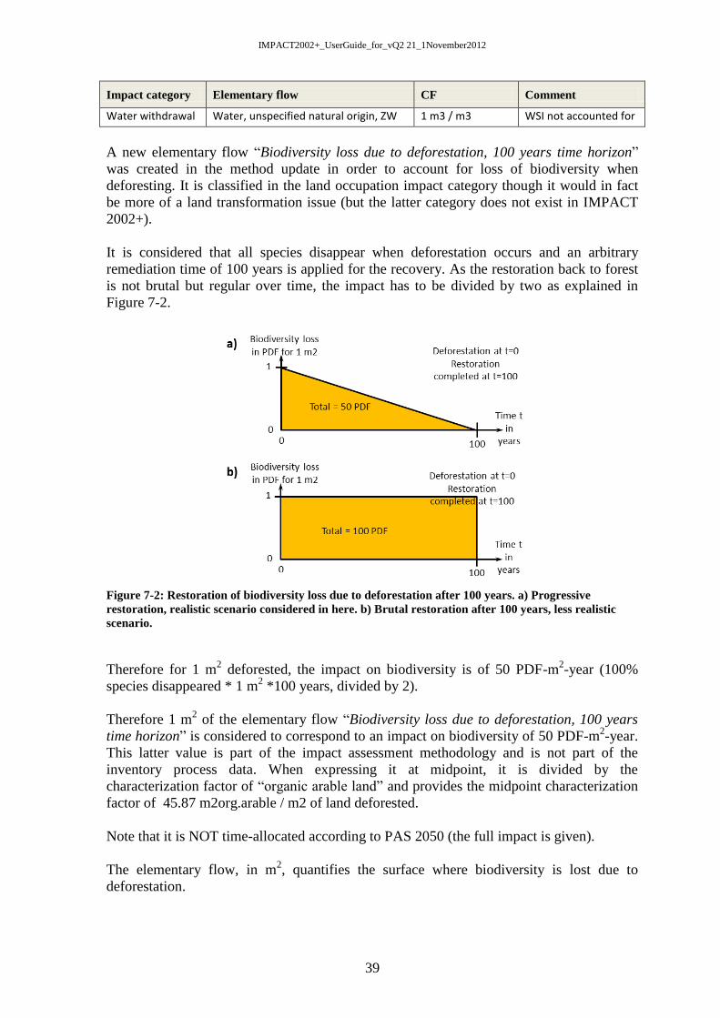
IMPACT2002+_UserGuide_for_vQ2 21_1November2012
39
Impact category Elementary flow CF Comment
Water withdrawal Water, unspecified natural origin, ZW 1 m3 / m3 WSI not accounted for
A new elementary flow “Biodiversity loss due to deforestation, 100 years time horizon”
was created in the method update in order to account for loss of biodiversity when
deforesting. It is classified in the land occupation impact category though it would in fact
be more of a land transformation issue (but the latter category does not exist in IMPACT
2002+).
It is considered that all species disappear when deforestation occurs and an arbitrary
remediation time of 100 years is applied for the recovery. As the restoration back to forest
is not brutal but regular over time, the impact has to be divided by two as explained in
Figure 7-2.
Figure 7-2: Restoration of biodiversity loss due to deforestation after 100 years. a) Progressive
restoration, realistic scenario considered in here. b) Brutal restoration after 100 years, less realistic
scenario.
Therefore for 1 m2 deforested, the impact on biodiversity is of 50 PDF-m
2-year (100%
species disappeared * 1 m2 *100 years, divided by 2).
Therefore 1 m2 of the elementary flow “Biodiversity loss due to deforestation, 100 years
time horizon” is considered to correspond to an impact on biodiversity of 50 PDF-m2-year.
This latter value is part of the impact assessment methodology and is not part of the
inventory process data. When expressing it at midpoint, it is divided by the
characterization factor of “organic arable land” and provides the midpoint characterization
factor of 45.87 m2org.arable / m2 of land deforested.
Note that it is NOT time-allocated according to PAS 2050 (the full impact is given).
The elementary flow, in m2, quantifies the surface where biodiversity is lost due to
deforestation.

IMPACT2002+_UserGuide_for_vQ2 21_1November2012
40
This elementary flow was created by Quantis, on November 2012, for IMPACT 2002+
vQ.2.21, to assess biodiversity loss on the scale of PDF.m2.yr.
The user needs to enter the inventory flow (in m2 deforested per functional unit) already
allocated over the number of years over which the deforestation has to be allocated (20
years by default, to be consistent with PAS 2050).