immigration, unemployment and gdp in the host country ... · centre d’economie de la sorbonne...

HAL Id: halshs-00800970https://halshs.archives-ouvertes.fr/halshs-00800970

Submitted on 14 Mar 2013

HAL is a multi-disciplinary open accessarchive for the deposit and dissemination of sci-entific research documents, whether they are pub-lished or not. The documents may come fromteaching and research institutions in France orabroad, or from public or private research centers.

L’archive ouverte pluridisciplinaire HAL, estdestinée au dépôt et à la diffusion de documentsscientifiques de niveau recherche, publiés ou non,émanant des établissements d’enseignement et derecherche français ou étrangers, des laboratoirespublics ou privés.

Immigration, unemployment and GDP in the hostcountry: Bootstrap panel Granger causality analysis on

OECD countriesEkrame Boubtane, Dramane Coulibaly, Christophe Rault

To cite this version:Ekrame Boubtane, Dramane Coulibaly, Christophe Rault. Immigration, unemployment and GDP inthe host country: Bootstrap panel Granger causality analysis on OECD countries. 2013. �halshs-00800970�

https://halshs.archives-ouvertes.fr/halshs-00800970

https://hal.archives-ouvertes.fr

Documents de Travail du Centre d’Economie de la Sorbonne

Immigration, unemployment and GDP in the host country :

Bootstrap panel Granger causality analysis

on OECD countries

Ekrame BOUBTANE, Dramane COULIBALY, Christophe RAULT

2013.14

Maison des Sciences Économiques, 106-112 boulevard de L'Hôpital, 75647 Paris Cedex 13 http://centredeconomiesorbonne.univ-paris1.fr/bandeau-haut/documents-de-travail/

ISSN : 1955-611X

Immigration, unemployment and GDP in the host

country: Bootstrap panel Granger causality

analysis on OECD countries∗

Ekrame Boubtane

CES-University Paris 1 and CERDI-University of Auvergne

Dramane Coulibaly

EconomiX-CNRS, University of Paris Ouest

Christophe Rault

LEO - University of Orleans and Toulouse Business School, France

Abstract

This paper examines the causality relationship between immigra-tion, unemployment and economic growth of the host country. Weemploy the panel Granger causality testing approach of Konya (2006)that is based on SUR systems and Wald tests with country specificbootstrap critical values. This approach allows to test for Granger-causality on each individual panel member separately by taking intoaccount the contemporaneous correlation across countries. Using an-nual data over the 1980-2005 period for 22 OECD countries, we findthat, only in Portugal, unemployment negatively causes immigration,while in any country, immigration does not cause unemployment. Onthe other hand, our results show that, in four countries (France, Ice-land, Norway and the United Kingdom), growth positively causes im-migration, whereas in any country, immigration does not cause growth.

Keywords: Immigration, growth, unemployment, causality.JEL classification: E20, F22, J61.

∗We are very grateful to two anonymous referees for their useful comments and sug-gestions. This paper was written while the second author was researcher at CEPII. Theauthors wish to thank Agnes Benassy-Quere, Agnes Chevallier, Gunther Capelle-Blancard,Christophe Destais, Lionel Fontagne and Lionel Ragot for their many helpful commentson a previous version of this paper. The usual disclaimer applies.

1

Documents de Travail du Centre d'Economie de la Sorbonne - 2013.14

1 Introduction

During the last decades, most OECD countries experienced an increase in in-ternational migration. Indeed, the number of immigrants received in OECDcountries substantially increased in the last decades, from about 82 millionsin the 1990 to 127 million in the 2010 (United Nation, 2009). Immigrantsare the main source of population growth in the OECD countries. Theycontribute more and more to population growth, compared to natural in-crease (the excess of births over deaths), particularly in European countriesduring the last years (Figure 1). In the context of the aging population andthe shrinking working age population, migration flows are likely to continueat a sustained pace in the next decades.

010

020

030

040

0Au

stra

liaAu

stria

Belg

ium

Can

ada

Den

mar

kFi

nlan

dFr

ance

Ger

man

yG

reec

eIc

elan

dIre

land

Italy

Luxe

mbo

urg

Net

herla

nds

New

Zea

land

Nor

way

Portu

gal

Spai

nSw

eden

Switz

erla

nd

Uni

ted

King

dom

Uni

ted

Stat

es

Natural increase Net migration

Figure 1: Components of population change, 1980-2005 (Variables are ex-pressed per 1,000 population). Temporary immigration flows are excluded.Source: Authors’ calculation, Labour Force Statistics, OECD (2010)

However, there is a public and political concern about the impact of theinternational migration on economic conditions in the receiving countries.Economists have studied, both theoretically and empirically, the impact ofimmigration on a variety of host country outcomes1 and also how economic

1See Okkerse (2008) and Keer and Keer (2011) for a review of literature.

2


conditions in the receiving countries affect migration flows.Theoretical studies (Johnson, 1980; Grossman, 1982) on the impact of

immigration on labour market in host countries show that the effects of im-migrants on the employment of residents depend on whether immigrants andnatives are substitutes or complements in production. Generally, the empir-ical studies on the impact of immigration on labour market in host countriesconclude that migration flows do not reduce the labour market prospects ofnatives (Simon et al., 1993; Pischke and Velling, 1997; Dustmann et al.,2005).

Theoretical studies on the effect of immigration on growth show that ifmigrants are skilled an inflow of migrants will have a less negative effect ongrowth compared to the natural increase in population (Dolado et al., 1994;Barro and Sala-i-Martin, 1995). This result is corroborated by the findingsfrom the empirical papers (Dolado et al., 1994; Ortega and Peri, 2009).

Some empirical papers have examined the causality between immigrationand unemployment and growth on data from different countries (Pope andWithers, 1985; Marr and Siklos, 1994; Islam, 2007; Morley, 2006). The ideais based on the fact that migrants take into account job opportunities intheir decision to migrate and the economic conditions are likely to have asignificant impact on migrations policies. Generally, the empirical paperson the causal link between immigration and host economic activity find noevidence of migration causing unemployment and growth, but find evidenceof causation running in the opposite direction.

This paper contributes to the existing literature on immigration by in-vestigating the causality relationship between immigration and host countryeconomic conditions (unemployment and growth) using the panel Grangercausality testing approach recently developed by Konya (2006) that is basedon SUR systems and Wald tests with country specific bootstrap critical val-ues. This approach allows to test for Granger-causality on each individualpanel member separately by taking into account the contemporaneous cor-relation across countries. Therefore, for each country, it allows to test forthe causality relationship between immigration and host economic variablesdepending on immigration policy.

We use annual data over the 1980-2005 period for 22 OECD countrieswhich are the major host countries (Figure 1). Our study provides evidencethat immigration does not cause host economic conditions (unemploymentand income per capita) and the influence of host economic conditions onimmigration depends on the host country. Indeed, on the one hand, ourfinding suggests that, only in Portugal, unemployment negatively Grangercauses immigration inflow, while in any country, immigration inflow doesnot Grange cause unemployment. On the other, our results indicate that,in four countries (France, Iceland, Norway and the United Kingdom), eco-nomic growth positively Granger causes immigration inflow, while in anycountry, immigration inflow does not Granger cause economic growth. This

3


heterogeneity in the influence of host economic conditions on immigrationcan be related to the characteristics of host country immigration policies.

The remainder of the paper is organized as follows. The existing litera-ture on the interaction between immigration, unemployment and growth isreviewed in Section 2. Section 3 presents the econometric methodology. Sec-tion 4 describes the data and reports the empirical results. Finally, Section5 offers some concluding remarks.

2 Literature review

Since the early 1980s a considerable literature on immigration has beendeveloped. The main concern is about the effect of immigration on labourmarket and economic growth in the host country.

Theoretical papers by Johnson (1980), Borjas (1987), Schmidt et al.(1994) and Greenwood and Hunt (1995) show that the effects of immigrantson the employment of residents depend on whether immigrants and nativesare substitutes or complements in production. If the labour suppliers ofresidents and recent immigrants are substitutes, an inflow of immigrants willreduce wages (assuming wage adjustment to clear the labour market) andwill increase the total employment. If labour force participation rates aresensitive to real wage rates, part of adjustment will occur through residentemployment. So, immigration may cause unemployment among natives whoare not willing to work at this lower wages. On the contrary, if residentsand immigrant workers are complements in production (immigrants maybe particularly adept at some types of jobs) the arrival of new immigrantsmay increase resident productivity and then raise their wages and theiremployment opportunities.

Generally, empirical studies on the impact of immigration on labourmarket in host countries conclude that migration flows do not reduce thelabour market prospects of natives. For example, the empirical studies basedon the spatial correlation approach (Simon et al., 1993 for the U.S; Pischkeand Velling, 1997 for Germany; Dustmann et al., 2005 for the U.K.) findno adverse effects of immigration on native unemployment. This result iscorroborated by findings from the studies based on natural experiments, i.e.,immigration caused by political rather than economic factors (Card, 1990 forthe Mariel Boatlift2 and Hunt, 1992 for the return of “pieds-noirs” in Franceafter the independence of Algeria). Contrary to the studies mentioned abovethat are conducted at the country level, Angrist and Kugler (2003) usea panel of 18 European countries from 1983 to 1999 and find a slightlynegative impact of immigrants on native labour market employment. Jean

2In 1980, Fidel Castro permitted any any person wished to leave Cuba free access todepart from the port of Mariel. Approximately, 125000 Cubans, mostly unskilled workers,migrated to Miami. As a result, Miami’s labour force increased by 7 percent.

4


and Jimenez (2007) evaluate the unemployment impact of immigration (andits link with output and labour market policies) in 18 OECD countries overthe period 1984 to 2003, and they do not find any permanent effect ofimmigration.

Some theoretical works (Dolado et al., 1994; Barro and Sala-i-Martin,1995) use a Solow growth model augmented by human capital to analyze theeffects of immigrants on growth. They conclude that the effects of migrationon economic growth depend on the skill composition of immigrants. Themore migrants are educated, the more immigration has a positive effect onthe economic growth in the host country.

Estimating an augmented Solow model on data from OECD economiesduring the 1960-1985 period, Dolado et al. (1994) find empirical evidencethat corroborates its theoretical result. Their empirical result shows thatbecause of their human capital content, migration inflows have less than halfthe negative impact of comparable natural population increases. However,more recently, Ortega and Peri (2009) estimate a pseudo-gravity model on14 OECD countries over the period 1980 to 2005 and find that immigrationdoes not affect income per capita.

A number of studies evaluate the fiscal impacts of immigration to exam-ine whether immigration burdens the host country’s social welfare systemsmore than is covered by the taxes paid by the immigrants (Auerbach andOreopoulos, 1999; Borjas, 1995, 2001; Passel and Clark, 1994). These stud-ies generally conclude that the total economic impact on the host countryis relatively small.

Since migrants take into account job opportunities in their decision tomigrate and because the economic conditions in host countries are likelyto have a significant impact on migration policies, some empirical papersexamine whether the migration flows respond to host country economicconditions. Particularly, some previous papers examine the Granger causal-ity links between immigration and unemployment using data on individualcountry (Pope and Withers, 1985 for Australia; Marr and Siklos, 1994 andIslam, 2007 for Canada). They find no evidence of migration causing higheraverage rates of unemployment, but find evidence of causation running in theopposite direction. However, Shan et al. (1999) find no Granger-causalitybetween immigration and unemployment, using data from Australia andNew Zealand. Morley (2006) finds evidence of a long-run Granger causalityrunning from per capita GDP to immigration on data for Australia, Canadaand the USA.

Contrary to these previous empirical papers that examine the Grangercausality between immigration and unemployment and growth using dataon individual country, we employ here panel Granger causality techniquesfor a panel of OECD countries. We use the panel Granger causality testingapproach of Konya (2006) that is based on SUR systems and Wald testswith country specific bootstrap critical values. Firstly, since country spe-

5


cific bootstrap critical values are generated, this approach allows to testfor Granger-causality on each individual panel member separately by tak-ing into account the possible contemporaneous correlation across countries.Generating country specific bootstrap critical values allows not to implementpretesting for unit roots and cointegration. Finally, bootstrapping providesa way to account for the distortions caused by small samples.

3 Econometric methodology

Three approaches can be implemented to test for Granger-causality in apanel framework. The first one is based on the Generalized Method of Mo-ments (GMM) that estimates (homogeneous) panel model by eliminatingthe fixed effect. However, it does not account for neither heterogeneity norcross-sectional dependence3. A second approach that deals with heterogene-ity was proposed by Hurlin (2008), but its main drawback is that the possiblecross-sectional dependence is not taken into account. The third approachdeveloped by Konya (2006) allows to account for both cross-sectional de-pendence and heterogeneity. It is based on Seemingly Unrelated Regression(SUR) systems and Wald tests with country specific bootstrap critical valuesand enables to test for Granger-causality on each individual panel memberseparately, by taking into account the possible contemporaneous correlationacross countries. Given its generality, we will implement this last approachin this paper.

The panel causality approach by Konya (2006) that examines the re-lationship between Y and X can be studied using the following bivariatefinite-order vector autoregressive (VAR) model:

yi,t = α1,i +ly1∑

s=1

β1,i,syi,t−s +lx1∑

s=1

γ1,i,sxi,t−s + ε1,i,t

xi,t = α2,i +ly2∑

s=1

β2,i,syi,t−s +lx2∑

s=1

γ2,i,sxi,t−s + ε2,i,t

(1)

where the index i (i = 1, ..., N) denotes the country, the index t (t =1, ..., T ) the period, s the lag, and ly1, lx1, ly2 and lx2 indicate lag lengths.The error terms, ε1,i,t and ε2,i,t are supposed to be white-noises (i.e. theyhave zero means, constant variances and are individually serially uncorre-lated) and may be correlated with each other for a given country. Moreover,it is assumed that Y and X are stationary or cointegrated so, depending onthe time-series properties of the data, they might denote the level, the firstdifference or some higher difference.

3Moreover, as shown by Pesaran et al. (1999) the GMM estimators can lead to in-consistent and misleading estimated parameters unless the slope coefficients are in factidentical.

6


We consider two bivariate systems. In the former system System 1 :(Y = U,X = M) where U and M denote unemployment rate and netmigration rate, respectively. In the latter System 2 : (Y = LGDP,X = M),where LGDP denotes the natural logarithm of per capita real GDP (or realincome).4

With respect to system (1) for instance, in country i there is one-wayGranger-causality running from X to Y if in the first equation not all γ1,i’sare zero but in the second all β2,i’s are zero; there is one-way Granger-causality from Y to X if in the first equation all γ1,i’s are zero but in thesecond not all β2,i’s are zero; there is two-way Granger-causality between Yand X if neither all β2,i’s nor all γ1,i’s are zero; and there is no Granger-causality between Y and X if all β2,i’s and γ1,i’s are zero.

Since for a given country the two equations in (1) contain the same pre-determined, i.e. lagged exogenous and endogenous variables, the OLS esti-mators of the parameters are consistent and asymptotically efficient. Thissuggests that the 2N equations in the system can be estimated one-by-one,in any preferred order. Then, instead of N VAR systems in (1), we canconsider the following two sets of equations:

y1,t = α1,1 +ly1∑

s=1

β1,1,sy1,t−s +lx1∑

s=1

γ1,1,sx1,t−s + ε1,1,t

y2,t = α1,2 +ly1∑

s=1

β1,2,sy2,t−s +lx1∑

s=1

γ1,2,sx2,t−s + ε1,2,t

...

yN,t = α1,2 +ly1∑

s=1

β1,N,syN,t−s +lx1∑

s=1

γ1,N,sxN,t−s + ε1,N,t

(2)

and

x1,t = α2,1 +ly2∑

s=1

β2,1,sy1,t−s +lx2∑

s=1

γ2,1,sx1,t−s + ε2,1,t

x2,t = α2,2 +ly2∑

s=1

β2,2,sy2,t−s +lx2∑

s=1

γ2,2,sx2,t−s + ε2,2,t

...

xN,t = α2,N +ly2∑

s=1

β2,N,sy2,t−s +lx2∑

s=1

γ2,N,sxN,t−s + ε2,N,t

(3)

Compared to (1), each equation in (2), and also in (3), has differentpredetermined variables. The only possible link among individual regres-sions is contemporaneous correlation within the systems. Therefore, system2 and 3 must be estimated by (SUR) procedure to take into account contem-poraneous correlation within the systems (in presence of contemporaneous

4Since per capita real GDP grows exponentially, it is taken in logarithm.

7


correlation the SUR estimator is more efficient than the OLS one). Follow-ing Konya (2006), we use country specific bootstrap Wald critical values toimplement Granger causality5. Generating bootstrap Wald critical allowsY and X not to be necessary stationary, they can denote the level, the firstdifference or some higher difference.

This procedure has several advantages. Firstly, it does not assume thatthe panel is homogeneous, so it is possible to test for Granger-causality oneach individual panel member separately by taking into account the possiblecontemporaneous correlation across countries. Therefore, for each country,it allows to test the causality relationship between immigration and host eco-nomic variables depending on immigration policy. Secondly, this approachwhich extends the framework by Phillips (1995) by generating country spe-cific bootstrap critical values does not require pretesting for unit roots andcointegration. This is an important feature since unit-root and cointegra-tion tests in general suffer from low power, and different tests often lead tocontradictory results. Finally, bootstrapping provides a way to account forthe distortions caused by small samples.

To check the robustness of our results, we consider two trivariate speci-fications. However, our focus will remain on the bivariate, one-period-aheadrelationship between migration and unemployment or per capita GDP, sowe will not consider the possibility of two variables jointly causing the thirdone. In the former System 3 : (Y = U,X = M,Z = LGDP ), whentesting for the causality between migration and unemployment, GDP percapita is treated as an auxiliary variable; whereas in the latter System 4 :(Y = LGDP,X = M,Z = U) when testing for the causality between mi-gration and GDP per capita, unemployment is treated as an auxiliary vari-able. Therefore, the trivariate specifications allows to test for the causalitybetween migration and unemployment, or GDP per capita by taking intoaccount the correlation between unemployment and economic growth. Forthe trivariate systems, the corresponding augmented variants of (2) and (3)are

y1,t = α1,1 +ly1∑

s=1

β1,1,sy1,t−s +lx1∑

s=1

γ1,1,sx1,t−s +lz1∑

s=1

λ1,1,sz1,t−s + ε1,1,t

y2,t = α1,2 +ly1∑

s=1

β1,2,sy2,t−s +lx1∑

s=1

γ1,2,sx2,t−s +lz1∑

s=1

λ1,2,sz2,t−s + ε1,2,t

...

yN,t = α1,N +ly1∑

s=1

β1,N,syN,t−s +lx1∑

s=1

γ1,N,sxN,t−s +lz1∑

s=1

λ1,N,szN,t−s + ε1,N,t

(4)and

5See Appendix for the procedure regarding how bootstrap samples are generated foreach country.

8


x1,t = α2,1 +ly2∑

s=1

β2,1,sy1,t−1 +lx2∑

s=1

γ2,1,sx1,t−s +lz2∑

s=1

λ2,1,sz1,t−s + ε2,1,t

x2,t = α2,2 +ly2∑

s=1

β2,2,sy2,t−1 +lx2∑

s=1

γ2,2,sx2,t−s +lz2∑

s=1

λ2,2,sz2,t−s + ε2,2,t

...

xN,t = α2,N +ly2∑

s=1

β2,N,sy2,t−1 +lx2∑

s=1

γ2,N,sxN,t−s +lz2∑

s=1

λ2,N,szN,t−s + ε2,N,t

(5)

4 Data and Econometric investigation

We use annual data over the period 1980 to 2005 for 22 OECD countries6

which are the major host countries. We use net migration, because, asmentioned by OECD, the main sources of information on migration varyacross countries. This may pose problem for the comparability of availabledata on inflows and outflows. Since the comparability problem is generallycaused by short-term movements, as argued by OECD (2009), taking netmigration tends to eliminate these movements that are the main source ofnon-comparability. Besides, compared to data on inflows and outflows, forthe countries that we consider, there are long available series on data on netmigration. Net migration rate is measured as total annual arrivals less totaldepartures, divided by the total population. Net migration data includeimmigrants from OECD countries and do not make a distinction betweennationals and foreigners. Entries of persons admitted on a temporary basisare not included in this statistic. Only permanent and long-term movementsare considered7. Real GDP (in 2000 Purchasing Power Parities) per capitais used to measure real income. The unemployment rate is the ratio of thelabour force that actively seeks work but is unable to find work. All variablesare taken from OECD Databases. Table 1 reports summary statistics ofvariables. The figures in Table 1 show that, on average, immigration rateincreased from 0.92 per thousand during the period 1980-1984 to 4.57 perthousand during the 2000-2005 period. At the same time, GDP per capitaincreased, whereas it is difficult to point out a decrease or an increase inunemployment rate.

Since the results from the causality test may be sensitive to lag structure,determining optimal lag length(s) is crucial for the robustness of findings.For a relatively large panel, equation- and variable-varying lag structure

6The sample includes: Australia, Austria, Belgium, Canada, Denmark, Finland,France, Germany, Greece, Ireland, Iceland, Italy, Luxembourg, Netherlands, New Zealand,Norway, Spain, Sweden, Switzerland, Portugal, United Kingdom and United States.

7Unauthorized migrants are not taken into account at the time of arrival. They maybe included when they are regularized and obtain a long-term status in the country.

9


Table 1: Descriptive statistics of 22 OECD countries

Period Immigration Unemployment GDP per capitarate (in thousand) rate (in percent) (2000 PPP)

1980-1984 0.9251 6.81 185891985-1989 1.4407 7.22 209461990-1994 3.4877 8.17 228681995-1999 2.8396 7.95 254602000-2005 4.5671 6.05 29288

would lead to an increase in the computational burden substantially. Toovercome this problem, following Konya (2006) we allow maximal lags todiffer across variables, but to be the same across equations. We estimatethe system for each possible pair of ly1, lx1, ly2, and lx2 respectively byassuming from 1 to 4 lags and then choose the combinations minimizing theAkaike Information Criterion (AIC). The AIC selects the following lags: inthe first bivariate system ly1 = 2, lx1 = 1, ly2 = 1, and lx2 = 1; and in thesecond one ly1 = 2, lx1 = 1, ly2 = 1 and lx2 = 2. In the first trivariatesystem, we take ly1 = 2, lx1 = 1, lz1 = 1, ly2 = 1, lx2 = 1 and lz2 = 1; andin the second one ly1 = 2, lx1 = 1, lz1 = 1, ly2 = 1, lx2 = 2 and lz2 = 1.

As mentioned above, testing for the cross-sectional dependence in a panelcausality study is crucial for selecting the appropriate estimator. FollowingKonya (2006) and Kar et al. (2010), to investigate the existence of cross-sectional dependence we employ three different tests: Lagrange multipliertest statistic of Breusch and Pagan (1980) for cross-sectional dependenceand two cross-sectional dependence tests statistic of Pesaran (2004), onebased on Lagrange multiplier and the other based on the pair-wise correla-tion coefficients.The Lagrange multiplier test statistic for cross-sectional dependence of Breuschand Pagan (1980) is given by:

CDBP = TN−1∑

i=1

N∑

j=i+1

ρ2ij (6)

where ρij is the estimated correlation coefficient among the residuals ob-tained from individual OLS estimations. Under the null hypothesis of nocross-sectional dependence with a fixed N and large T, CDBP asymptoti-cally follows a chi-squared distribution with N(N − 1)/2 degrees of freedom(Greene (2003), p.350).Since, BP test has a drawback (indiquer lequel ?Dramane) when N islarge, Pesaran (2004) proposes another Lagrange multiplier (CDLM ) statis-tic for cross-sectional dependence that does nor suffer from this problem.The CDLM statistic is given as follows:

10


Table 2: Results for cross-sectional dependence tests

Bivariate systemModel CDBP CDLM CD

System 1 (U) 450.7726*** 10.2246*** 83.1740***(0.000) (0.000) (0.000)

System 1 (M) 280.7111** 2.3128** 35.8008***(0.014) (0.021) (0.000)

System 2 (LGDP) 709.8659*** 22.2789*** 131.8569***(0.000) (0.000) (0.000)

System 2 (M) 308.4733** 3.6044*** 12.2688***(0.000) (0.000) (0.000)

Trivariate systemModel CDBP CDLM CD

System 3 (U) 449.2574*** 10.1543*** 89.0142***(0.000) (0.000) (0.000)

System 3 (M) 308.1410 3.5889 3510(0.001) (0.000) (0.000)

System 4 (LGDP) 634.9612*** 18.7940*** 120.2349***(0.000) (0.000) (0.000)

System 4 (M) 326.7683** 4.4556*** 6.1835***(0.000) (0.000) (0.000)

U , M and LGDP denote unemployment rate, net migration rate and natu-ral logarithm of per capita real GDP, respectively. CDBP , CDLM and CDdenote respectively the test statistic of Breusch and Pagan Lagrange mul-tiplier statistic for cross-sectional dependence, Pesaran Lagrange multiplierstatistic for cross-sectional dependence, and Pesaran cross-sectional depen-dence statistic based on the pair-wise correlation coefficients. Under thenull hypothesis of no cross-sectional dependence, CDBP follows a chi-squaredistribution with N(N − 1)/2 degrees of freedom, CDLM and CD followstandard normal distribution . ***, ** and * indicate rejection of the nullhypothesis at 1 and 5 and 10 percent level of significance, respectively.

CDLM =

√

1

N(N − 1)

N−1∑

i=1

N∑

j=i+1

(T ρ2ij − 1) (7)

Under the null hypothesis of no cross-sectional dependence with the firstT → ∞ and then N → ∞ , CDLM asymptotically follows a normal dis-tribution. However, this test is likely to exhibit substantial size distortionswhen N is large relative to T. To tackle this issue, Pesaran (2004) proposesa new test for cross-sectional dependence (CD) that can be used where Nis large and T is small. This test is based on the pair-wise correlation coef-ficients rather than their squares used in the LM test. The CD statistic isgiven by:

11


CD =

√

2T

N(N − 1)

N−1∑

i=1

N∑

j=i+1

ρij (8)

Under the null hypothesis of no cross-sectional dependence with the T →

∞ and then N → ∞ in any order, CD asymptotically follows a normaldistribution. Pesaran (2004) show that the CD test is likely to have goodsmall sample properties (for both N and T small).

Tables 2 reports the results of these cross-sectional dependence tests.The results in 2 show that, for bivarriate and trivariate systems, all the threetests reject the null of no cross-sectional dependence across the membersof the panel at 5% level of significance, implying that the SUR methodis appropriate rather than a country-by-country OLS estimation. Cross-sectional dependence tests confirm that strong economic links exist betweenOECD countries members.

5 Results and Discussion

Tables 3-6 report the results of Granger causality. Notice that the bootstrapcritical values are substantially higher than the chi-square critical ones usu-ally applied with the Wald test, and that they vary considerably from acountry to another and across tables8. This reflects Christophe proposede supprimer (the stationary property of the series and) Dramaneconfirmation? the cross-section dependance.

The results of causality tests from immigration to unemployment andfrom unemployment to immigration are displayed in Table 3 and Table 4,respectively. The results of causality from immigration to per capita GDPand from GDP per capita to immigration are displayed in Table 5 and Table6, respectively. In tables 3-6, the column ‘estimated coefficient’ representsthe estimated coefficient of xt−1 (yt−1) in the equation testing from Grangercausality from X to Y (Y to X). Since, in each case, in testing from Grangercausality from X to Y (Y to X), we have only one lag for X (Y ), thisestimated coefficient represent both the short run and the long impact.

The results in Table 3 show that, in any country, there is no causalityfrom immigration to unemployment. Table 4 shows that, for only Portugal,there is a significant (at the 10% level of significance) negative causalityrunning from unemployment to immigration, whereas for the other countriesthere is no significant causality running from unemployment to immigration.

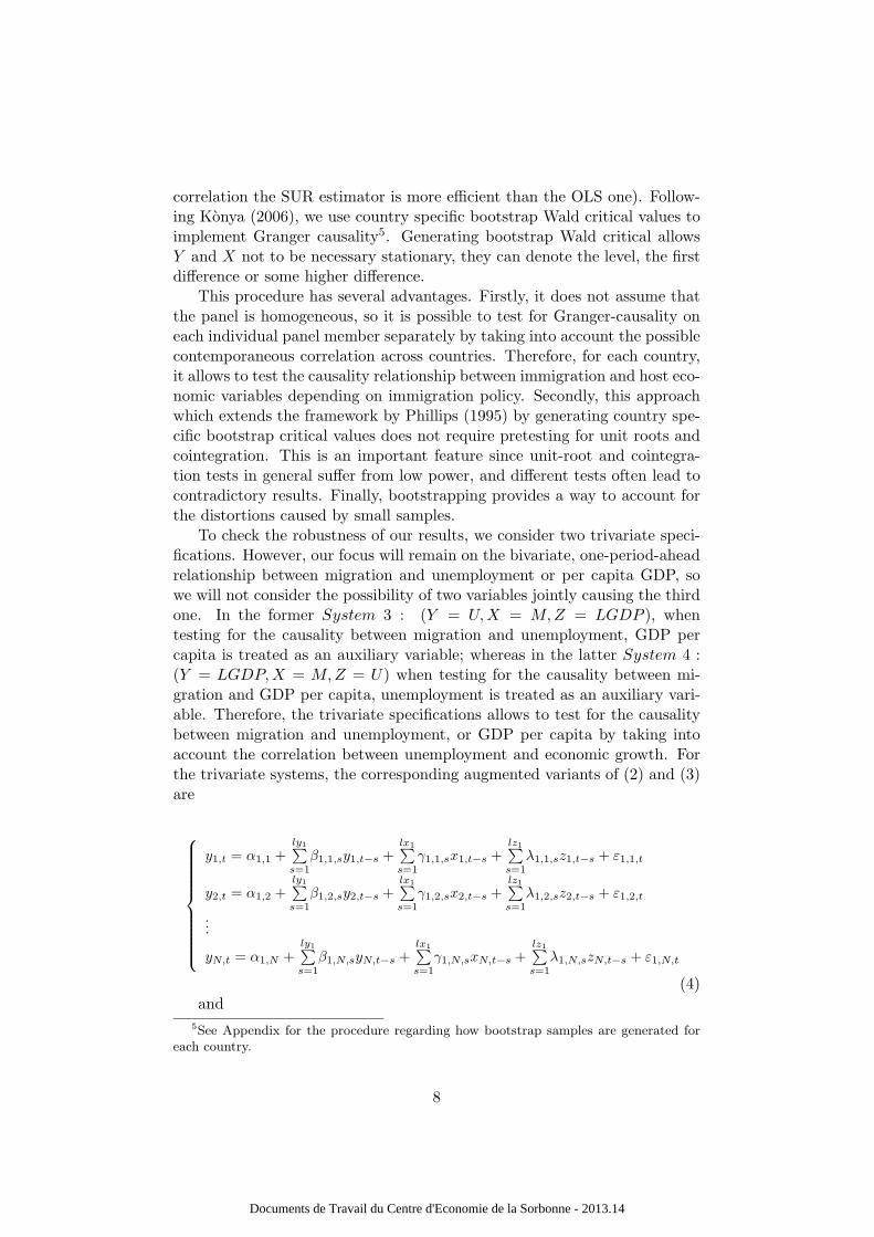
The results in Table 5 suggest that, in any country, there is no signif-icant causality running from immigration to GDP. Table 6 shows that infour countries (France, Iceland, Norway and the United Kingdom) there is a

8The chi-square critical values for one degree of freedom, i.e. for Wald tests with onerestriction, are 6.6349, 3.8415, 2.7055 for 1%, 5% and 10%, respectively.

12


Table 3: Granger causality tests from immigration to unemployment - bi-variate modelCountry Estimated Test Stat. Bootstrap critical values

coefficient 1% 5% 10%

Australia 0.1938 13.0198 287.7363 138.7766 90.6493Austria 0.0234 5.6799 286.6355 125.8565 80.5467Belgium -0.1245 3.6805 175.4215 77.6084 50.1208Canada 0.0059 0.0140 274.5667 139.4946 91.9954Denmark -0.2288 5.7721 337.5072 140.8359 90.8154Finland 1.2062 52.9716 316.3091 150.2173 96.7384France -0.0292 0.0222 173.9483 81.8138 52.8704Germany 0.0173 1.9601 295.8401 139.7354 93.7130Greece 0.0821 9.0246 230.2833 109.3694 72.4079Iceland 0.0610 15.7417 286.9114 132.6577 86.1520Ireland -0.1138 23.1385 342.9583 154.8923 103.2070Italy -0.0583 11.3306 207.7941 85.4204 54.6998Luxembourg 0.0072 2.4710 331.8680 159.0345 106.0899Netherlands 0.1967 11.7020 230.3935 99.0387 62.2805New Zealand -0.0130 0.4398 248.4385 112.1155 75.7471Norway 0.2627 58.7593 303.4181 134.9851 85.3963Portugal 0.0218 0.6693 156.7490 75.7666 49.2947Spain -0.2794 57.3525 241.2615 110.0584 72.6988Sweden 0.0373 1.2791 404.1338 196.2905 125.7544Switzerland 0.0767 35.3416 296.1276 143.5848 92.3061United Kingdom -0.1357 3.8144 263.5924 119.9834 77.9560United States -0.1908 7.7114 284.1708 132.2164 83.6499

Note: H0 : immigration does not cause unemployment. The column “Estimatedcoefficient” denotes the estimated coefficient of the lag of immigration rate in theequation testing for Granger causality from immigration to unemployment rate.Column “Test Stat.” represents the Wald test statistic for Granger causality fromimmigration to unemployment rate. ***, **, and * indicate the rejection of the nullhypothesis at the 1, 5, and 10 percent levels of significance, respectively.

13


Table 4: Granger causality tests from unemployment to immigration - bi-variate modelCountry Estimated Test Stat. Bootstrap critical values


Australia -0.3315 8.2290 306.8964 143.4189 93.5239Austria 0.0892 0.0347 326.9468 141.4868 90.3277Belgium -0.0858 13.4350 206.6685 90.3308 58.6337Canada -0.2170 6.5177 292.1500 125.6811 80.9669Denmark 0.1012 4.8414 350.6973 150.9016 100.5670Finland -0.0378 9.5450 273.6004 130.8957 85.1077France -0.0540 16.1243 290.4957 147.3383 99.4058Germany -0.0490 0.1187 294.3776 144.2217 95.1106Greece -0.0161 0.0375 341.1858 171.5095 111.4617Iceland -0.2756 1.1717 218.2504 100.4272 64.8144Ireland -0.3785 5.1142 244.2332 107.9090 69.3826Italy -0.1845 1.7309 369.5746 169.3226 113.8005Luxembourg 1.4298 5.7080 207.6518 99.2973 64.7285Netherlands 0.1746 16.5221 236.9243 124.0193 81.6781New Zealand 0.2662 1.7910 290.4320 134.6834 85.8611Norway 0.0597 0.3610 264.9229 119.5181 74.3819Portugal -0.6033 122.3191* 334.0911 146.9617 97.5169Spain -0.1282 6.1913 132.1068 59.5167 38.1426Sweden -0.0153 0.1089 232.5700 108.9333 69.3073Switzerland -0.5030 14.4276 241.6980 116.7093 76.3445United Kingdom -0.0364 0.6224 221.8538 102.3553 66.4853United States -0.0649 4.0023 314.9698 153.4151 100.2002

Note: H0 : unemployment does not cause immigration. Column “Estimatedcoefficient” denotes the estimated coefficient of the lag of unemployment rate inthe equation testing for Granger causality from unemployment to immigration.Column “Test Stat.” represents the Wald test statistic for Granger causality fromunemployment to immigration. ***, **, and * indicate the rejection of the nullhypothesis at the 1, 5, and 10 percent levels of significance, respectively.

14


Table 5: Granger causality tests from immigration to per capita GDP -bivariate modelCountry Estimated Test Stat. Bootstrap critical values


Australia -0.0062 145.2363 642.1363 300.2588 184.0594Austria -0.0014 20.1850 509.7105 216.5362 133.1134Belgium -0.0030 18.2444 681.2106 284.3846 186.9683Canada -0.0071 107.2464 908.8519 393.7506 258.2969Denmark -0.0000 0.0018 651.5292 255.4873 155.2668Finland -0.0223 136.2913 603.1720 268.2465 169.2409France -0.0207 103.0732 585.3197 304.6188 206.4012Germany 0.0004 7.8763 558.5621 269.2568 182.6525Greece -0.0007 0.6512 185.0076 83.9402 53.1138Iceland -0.0041 25.0658 528.0840 232.1546 141.7218Ireland -0.0016 23.6291 531.9374 223.8201 144.6197Italy -0.0004 1.1934 524.0714 244.2464 159.6062Luxembourg 0.0001 0.0160 475.9581 197.6779 119.3652Netherlands -0.0028 24.4681 609.2427 270.3311 176.1551New Zealand -0.0005 1.9322 528.0105 229.6578 144.5666Norway -0.0036 38.4940 883.3209 343.9916 215.0718Portugal -0.0010 1.0132 472.0737 216.6576 137.7028Spain -0.0000 0.0004 517.1960 249.8073 168.2989Sweden -0.0021 7.7808 704.4112 310.1129 197.6469Switzerland -0.0026 28.3606 491.3078 230.0392 150.7396United Kingdom -0.0039 24.8869 770.9085 344.2256 229.1871United States -0.0016 1.4538 638.4730 305.0717 199.0662

Note:H0 : immigration does not cause per capita GDP. Column “Estimated coeffi-cient” denotes the estimated coefficient of the lag of immigration rate in the equationtesting for Granger causality from immigration rate to log (per capita GDP). Column“Test Stat.” represents the Wald test statistic for Granger causality from immigra-tion rate to log(per capita GDP). ***, **, and * indicate the rejection of the nullhypothesis at the 1, 5, and 10 percent levels of significance, respectively.

15


Table 6: Granger causality tests from GDP per capita to immigration -bivariate modelCountry Estimated Test Stat. Bootstrap critical values


Australia 0.5966 0.2133 44.1132 21.2758 14.2802Austria 4.1763 3.0485 69.4796 31.4398 19.9934Belgium 2.2344 7.9633 165.3051 81.3064 53.7078Canada 4.7688 16.5011 67.4497 31.3532 20.3437Denmark 0.9893 0.5960 64.1267 29.2654 19.2426Finland 0.7857 4.5312 96.3905 45.0952 28.9216France 0.3803 14.5200* 38.4159 19.2248 12.9537Germany -1.9891 0.5180 103.0069 50.1292 32.2102Greece -1.6919 1.8655 190.9693 90.9634 60.1493Iceland 19.4588 72.6350** 78.6381 34.7857 21.7824Ireland 12.0384 37.9026 229.9758 104.5681 68.5805Italy 5.5991 7.6469 42.8646 21.7309 14.0878Luxembourg 2.1905 1.8097 77.9690 36.2650 22.8619Netherlands -1.3450 2.8127 57.4609 25.3127 16.4470New Zealand 14.6758 8.0079 70.7573 32.1478 20.4502Norway 4.9385 43.0513*** 42.8830 21.1842 13.4986Portugal 3.2272 19.6184 175.9970 80.2091 51.6689Spain 4.7815 13.5030 243.5550 128.0488 89.6999Sweden 1.4345 0.9856 66.7698 29.7692 19.2975Switzerland 3.9219 1.3726 93.4584 43.4481 27.4950United Kingdom 3.9982 34.5706** 66.1783 29.5176 18.6249United States 0.3443 0.4280 93.8299 42.5891 27.7797

Note: H0 : per capita GDP does not cause immigration. Column “Estimated coef-ficient” denotes the estimated coefficient of the lag of log (per capita GDP) in theequation testing for Granger causality from log(per capita GDP) to immigration rate.Column “Test Stat.” represents the Wald test statistic for Granger causality fromlog(per capita GDP) to immigration rate. ***, **, and * indicate the rejection of thenull hypothesis at the 1, 5, and 10 percent levels of significance, respectively.

16


positive significant causality running from GDP to immigration; while in theother countries there is no significant causality running from GDP to immi-gration. There is a positive causality running from GDP to immigration at1 percent level of significance for Norway, 5 percent level of significance forIceland and the United Kingdom Norway and 10 percent level of significancefor France.

17


Table 7: Granger causality tests from immigration to unemployment -trivariate modelCountry Estimated Test Stat. Bootstrap critical values


Australia -0.0236 0.2616 334.7989 149.5224 96.9316Austria 0.0000 0.0000 217.9372 95.8341 67.7080Belgium 0.2315 7.8663 239.4201 127.4790 88.2908Canada 0.0332 1.6553 301.0002 151.0504 94.8809Denmark -0.1222 2.1206 245.3595 118.8353 81.0714Finland 1.1832 60.0880 281.9510 159.2575 95.2094France 0.4630 2.9252 209.0307 98.4185 70.4652Germany -0.0683 21.2939 239.9914 124.7901 84.8816Greece 0.0730 6.5802 221.2246 99.5950 67.9572Iceland 0.0601 18.4297 173.9361 79.5713 52.5650Ireland -0.0140 0.1830 340.5097 174.8992 122.6541Italy -0.0338 1.7075 269.7529 118.0978 68.6167Luxembourg -0.0109 7.2257 323.5371 141.3815 98.4819Netherlands -0.1284 3.6164 234.9126 129.9640 83.6289New Zealand 0.0025 0.0227 216.0790 100.3512 67.0414Norway 0.2228 27.7386 198.0062 104.7487 65.6404Portugal 0.1705 38.8816 178.8365 88.6373 54.7418Spain -0.3758 40.2969 355.6600 159.9856 107.8534Sweden -0.0597 5.3803 271.3265 148.3409 101.0271Switzerland 0.0461 6.9727 284.6761 166.0940 113.5712United Kingdom 0.1884 13.7985 299.0586 177.7895 124.2034United States -0.1235 4.0838 185.7634 94.4119 60.1460

Note: H0 : immigration does not cause unemployment. The column “Estimatedcoefficient” denotes the estimated coefficient of lag of immigration rate in theequation testing for Granger causality from immigration to unemployment rate.Column “Test Stat.” represents the Wald test statistic for Granger causality fromimmigration to unemployment rate. ***, **, and * indicate the rejection of the nullhypothesis at the 1, 5, and 10 percent levels of significance, respectively.

18


Table 8: Granger causality tests from unemployment to immigration -trivariate modelCountry Estimated Test Stat. Bootstrap critical values


Australia -0.3544 7.4992 279.1272 112.9311 72.3312Austria -1.1704 4.7155 298.8886 129.4893 84.5797Belgium -0.0346 1.4860 242.8462 119.6951 89.1278Canada -0.0754 0.4910 188.0826 91.5665 61.4262Denmark 0.2585 32.4278 188.2056 118.6136 80.7883Finland -0.0561 22.5583 138.6604 72.7321 51.4282France -0.1242 64.9696 300.9184 155.5800 99.3673Germany 0.4609 4.6375 203.8046 109.3860 76.4460Greece 0.2199 4.5983 185.7841 97.2281 64.1550Iceland -0.9214 13.8203 107.5253 60.1570 38.9982Ireland -0.1921 2.1211 224.5771 110.0444 64.4107Italy -0.8811 41.1152 243.3718 132.7531 89.5198Luxembourg 1.1127 2.3414 177.9395 106.4410 71.6757Netherlands 0.6740 63.0093 189.7809 105.0316 75.0042New Zealand 0.5082 6.5117 191.1896 91.0532 61.8064Norway -0.2136 6.7821 159.1635 85.6986 56.1403Portugal -0.3488 19.2426* 258.8398 107.6579 13.2983Spain -0.3087 38.6889 249.8439 126.8201 82.2173Sweden -0.0442 0.6697 128.9744 75.5884 52.1674Switzerland -1.1771 82.4006 175.6078 102.6137 94.8856United Kingdom 0.0972 2.6250 205.7940 100.9149 66.4243United States -0.1923 14.9663 227.6817 118.0697 76.5009

Note: H0 : unemployment does not cause immigration. Column “Estimatedcoefficient” denotes the estimated coefficient of the lag of unemployment rate inthe equation testing for Granger causality from unemployment to immigration.Column “Test Stat.” represents the Wald test statistic for Granger causality fromunemployment to immigration. ***, **, and * indicate the rejection of the nullhypothesis at the 1, 5, and 10 percent levels of significance, respectively.

19


Table 9: Granger causality tests from immigration to GDP per capita -trivariate modelCountry Estimated Test Stat. Bootstrap critical values


Australia -0.0019 2.7210 263.0225 145.8187 95.8702Austria -0.0016 52.1135 176.8970 98.1363 70.2374Belgium -0.0013 1.4123 201.3232 113.9322 80.0250Canada -0.0036 49.2108 426.2160 207.6525 143.1817Denmark -0.0005 0.3593 236.7658 103.3482 69.9353Finland -0.0151 148.9112 354.1961 250.0251 165.7849France -0.0104 21.8196 217.7683 125.9724 84.1495Germany 0.0018 109.6546 359.8191 196.2351 117.6784Greece -0.0022 12.2776 84.4463 43.1847 30.1339Iceland -0.0037 55.9620 258.6184 108.5395 71.9754Ireland 0.0004 0.2885 314.5068 123.1126 84.9670Italy 0.0020 22.0193 247.4185 125.6980 78.8425Luxembourg 0.0004 0.2612 271.3135 102.4394 66.6438Netherlands 0.0002 0.0469 302.4367 138.8919 97.4181New Zealand -0.0012 7.2373 212.6498 97.5138 63.3307Norway -0.0007 0.8258 248.7915 131.7521 83.3682Portugal -0.0026 4.8777 252.3874 136.2109 89.8816Spain 0.0022 51.7245 360.7482 177.4140 113.8133Sweden -0.0005 0.3652 331.6734 166.9935 113.4156Switzerland -0.0021 38.1448 203.7382 104.0096 72.0211United Kingdom -0.0032 14.1634 390.5799 165.6081 106.3365United States 0.0038 5.1356 223.9490 123.8660 73.3980

Note:H0 : immigration does not cause per capita GDP. Column “Estimated coeffi-cient” denotes the estimated coefficient of the lag of immigration rate in the equationtesting for Granger causality from immigration rate to log(per capita GDP). Column“Test Stat.” represents the Wald test statistic for Granger causality from immigra-tion rate to log(per capita GDP). ***, **, and * indicate the rejection of the nullhypothesis at the 1, 5, and 10 percent levels of significance, respectively.

20


Table 10: Granger causality tests from GDP per capita to immigration -trivariate modelCountry Estimated Test Stat. Bootstrap critical values


Australia -0.1911 0.0193 33.1207 15.8983 10.5450Austria 4.7758 3.2613 57.7751 24.6857 17.7721Belgium 1.9504 4.6028 132.3694 54.3006 35.0875Canada 5.1178 14.6852 41.5492 20.1348 14.7413Denmark 3.4962 5.0764 59.8428 33.2786 21.2082Finland 1.0496 6.4777 52.4382 27.2489 16.6740France 0.5871 33.3279** 50.1890 20.1720 12.6587Germany 2.5736 0.5161 74.3589 36.0617 23.8127Greece 1.1091 0.6373 163.6991 73.3959 49.7018Iceland 24.8554 95.9432*** 36.1925 19.7481 13.4029Ireland 10.8065 29.0963 75.1909 35.3527 29.7500Italy 13.9791 100.5827 349.7739 220.4192 115.0919Luxembourg 3.7774 2.9931 63.2546 33.8113 20.9812Netherlands 4.3278 3.2520 84.4697 43.4926 29.1752New Zealand 15.9942 11.6162 38.2584 19.3498 12.3952Norway 5.6071 59.6025*** 31.2682 16.1885 10.7985Portugal 0.1791 0.0395 104.1727 42.8774 27.2084Spain 7.5361 31.3371 237.2832 96.6455 65.7927Sweden 2.0523 1.8519 58.4588 25.7216 17.3191Switzerland 29.7581 158.6569 397.1388 249.7637 162.9928United Kingdom 3.3460 8.5492* 28.8443 8.8169 4.8859United States -0.8556 1.3413 76.4092 32.2444 19.1393

Note: H0 : GDP does not cause immigration. Column “Estimated coefficient” denotesthe estimated coefficient of the lag of log (per capita GDP) in the equation testingfor Granger causality from log(per capita GDP) to immigration rate. Column “TestStat.” represents the Wald test statistic for Granger causality from log(per capitaGDP) to immigration rate. ***, **, and * indicate the rejection of the null hypothesisat the 1, 5, and 10 percent levels of significance, respectively.

21


To check the robustness of our findings, Tables 7-10 report the resultsusing a trivariate specification. In the trivariate specifications, the focuswill remain on the bivariate, one-period-ahead relationship between migra-tion and and unemployment or GDP per capita, so we will not study thepossibility of two variables jointly causing the third one. The results in Ta-bles 7-10 corroborate the findings from the bivariate specifications (exceptfor the significance level in some cases).

Our finding that immigration does not impact host economic variablessupports the results from some previous studies (Simon et al., 1993; Doladoet al., 1994; Marr and Siklos, 1994; Pischke and Velling, 1997; Dustmann etal., 2005 Ortega and Peri, 2009).

The result that immigration does not impact host GDP per capita canbe explained by the human capital content of migration inflow (Dolado etal., 1994). On the one hand, due to reduction in the capital/labour ratioin the host economy, increase in immigration (population) would leads toa decrease in output per capita. On the other hand, the more migrantsare educated, the more immigration has a positive effect on the economicgrowth of the host country. If immigrants have little human capital, thenegative impact caused by the reduction in the capital/labour ratio willdominate. If immigrant human capital levels are higher than natives’ by asufficient amount, immigration will increase output per capita. Therefore,our results suggest that, the human capital content of the migration inflowis high in order to compensate the negative effect caused by reduction inthe capital/labour ratio. As a result there will be no negative impact ofimmigration on growth and employment.

The result that immigration does not cause resident unemployment canbe explained as follows. According to theoretical models, the effects of immi-gration on wages and employment of host country residents, depend on theextent to which migrants are substitutes or complements to those of existingworkers (Borjas, 1995). If migrants and residents are substitutes, immigra-tion will decrease wages by increasing competition in the labour market.The extent to which declining wages increases unemployment or inactivityamong host country residents depends on the willingness of existing workersto accept lower wages. If, on the other hand, migrants are complementary tohost country residents, the arrival of new immigrants may increase residentproductivity and then raise their wages and their employment opportunities.Thus, our finding that immigration does not cause resident unemploymentreflects the fact there may be a coexistence of substitutability and comple-mentarity between migrants and residents. As mentioned by Orrenius andZavodny (2007), the degree of substitution between immigrants and nativesis likely to vary across skill levels and over time. In fact, substitution canoccur in industries with less skilled workers because employees are more in-terchangeable and training costs are lower than in industries with skilledworkers. Moreover, the differences in the quality and relevance of education

22


and experience acquired abroad make skilled immigrants less substitutablefor skilled natives.

For some countries, the particular findings of causality from immigrationto host economic variables can be related to their immigration policies. Inthe case of Portugal, the negative influence of unemployment on immigra-tion can be explained by the fact that the needs of Portuguese employersplay a significant role in the recruitment process of the newly arrived immi-grants. Moreover, both Portuguese nationals and foreigners are more likelyto immigrate to a third European country when the labour market situationis less favorable in Portugal.

In France, family component is the main channel of entry for long-termimmigrants. The positive influence of the economic growth on migrationflows may be related to family reunification requirements. In order to bringtheir families, immigrants have to satisfy a minimum level of income. Duringa period of higher growth, immigrants have great possibility to satisfy thisminimum level of income criteria. Moreover, economic migration to Francemainly includes immigrants from European countries (such as Portugal) thatare attracted by better economic prospects.

Norway and Iceland are two small countries with high incomes and highdemand for labour. So, the main attraction for immigrants to these twocountries is the high standard of living. A large percentage of labour im-migration is from Nordic neighbours and OECD countries. The boomingeconomy and the increased demand of labour in Norway and Iceland ledauthorities to allow the entry of labour migrants over the last years.

Finally, the explanation of the result for the United-Kingdom is as fol-lows. Immigrants to the United Kingdom are more attracted by the prospectof higher wages produced by the greater economic growth. In the UnitedKingdom, labour migration represents a sizable percentage of total inflows(44 percent in 2005)9. If family members accompanying workers are takeninto account, the percentage of economic migration is around 60 percentin 2005. The inflow of labour migration increased from 124 thousands onaverage per year in the 1980s to 200 thousands in the 1990s. From 2000 to2005, labour migration inflows reached 333 thousand per year on average.

6 Concluding Remarks

This paper has examined the causality between immigration and the eco-nomic conditions of host countries (unemployment and growth). We haveemployed the panel Granger causality testing approach recently developed

9The work category combines two reasons for migration in the International PassengerSurvey: “definite job” and “looking for work”. Authors’ calculation is based on Office forNational Statistics (2008); Office for National Statistics (2009).

23


by Konya (2006) that is based on SUR systems and Wald tests with countryspecific bootstrap critical values. We have used annual data over the 1980-2005 period for 22 OECD countries which are the major host countries.

Our study has provided evidence that immigration does not cause hosteconomic conditions (unemployment and income per capita) and the in-fluence of host economic conditions on immigration depends on the hostcountry. Indeed, on the one hand, our finding suggests that, only in Portu-gal, unemployment negatively Granger causes immigration inflow, while inany country, immigration inflow does not Granger cause unemployment. Onthe other hand, our results indicate that, in four countries (France, Iceland,Norway and United Kingdom), economic growth positively Granger causesimmigration inflow, whereas in any country, immigration inflow does notGranger cause economic growth. This heterogeneity in the influence of hosteconomic conditions on immigration can be related to the characteristics ofhost country immigration policies.

In order to tackle the problem of ageing population, many OECD coun-tries see immigration as a potential solution to compensate for labour short-age. Our results have revealed that immigration flows do not harm theemployment prospects of residents.

24


Appendix

A-1 The bootstrap procedure

The procedure to generate bootstrap samples and country specific criticalvalues (in the test of no causality from X to Y ) consists of the following fivesteps (Konya, 2006)

1st step: Implement an estimation of (2) under the null hypothesis of no-causality from X to Y by (i.e. imposing γ1,i,s = 0 the for all i and s) andget the corresponding residuals:

eH0,i,t = yi,t − αi,1 +

ly1∑

s=1

β1,i,syi,t−s

From these residuals, build the N × T [eH0,i,t] matrix.

2nd step: In order to preserve the contemporaneous dependence betweenerror terms in (2), randomly select a full column from [eH0,i,t] matrix at atime (i.e do not draw the residuals for each country one-by-one); and denote

the selected bootstrap residuals as[

e∗H0,i,t

]

where t = 1, ..., T ∗ and T ∗ can

be greater than T.

3rd step: Build the bootstrap sample of Y under the hypothesis of no-causality from X to Y, i.e. using the following formula:

y∗i,t = αi,1 +

ly1∑

s=1

β1,i,sy∗

i,t−s + e∗H0,i,t

4th step: Replace yi,t by y∗i,t, estimate (2) without any parameter restric-tions and then implement the Wald test for each country to test for theno-causality null hypothesis.

5th step: Develop the empirical distributions of the Wald test statisticsby repeating (10,000 replications) the steps 2-4 many times and build thebootstrap critical values.

A-2 Test for serial correlation in residual

Since each system (2) and (3) is estimated separately by accounting for con-temporaneous correlated within the system(Konya, 2006), for each systemwe implement separately a panel test for serial correlation (for each countryerror is assumed to be a white noise).

25


We employ a test for serial correlation in residual based on the ap-proach proposed by Wooldridge (2002), p. 282-283. Let εi,t be the resid-uals that are assumed to be white noises (i.e. with zero means, constantvariances and are individually serially uncorrelated) and contemporaneouscorrelated across countries: var(εi,t) = σ2

i , cov(εi,t, εi,s) = 0 for t 6= s,cov(εi,t, εj,t) = σ2

ij , for i 6= j.Let consider the errors uit = ∆εi,t. Under the assumptions on εi,t,

Corr(uit, ui,t−1) =cov(ui,t, ui,t−1)

√

var(ui,t)var(ui,t−1)=

−σ2i

√

(2σ2i )(2σ

2i )

= −0.5

To test for serial correlation in εi,t, Wooldridge (2002) propose to testρ = Corr(uit, ui,t−1) = −0.5 in the following regression of ui,t on ui,t−1

ui,t = ρui,t−1 + ηi,t

The errors ηi,t are heteroskedastic (because var(εi,t) = σ2i ), and contrary

to Wooldridge (2002), in our case, the errors ηi,t are cross-sectional corre-lated (because cov(εi,t, εj,t) 6= 0). Then, we implement the regression of ui,ton ui,t−1 using Feasible Generalized Least Squares (FGLS) estimation thatallows for heteroskedastic error structure with cross-sectional correlation.To test for ρ = −0.5, we use the Wald test statistic that follows, under thenull hypothesis, a chi-squared distribution with 1 degree of freedom.

The results of serial correlation test are reported in Table A-1.

26


Table A-1: Test for serial correlation in residualBivariate system

System Lag Length Test Statistic

(Y = U,X = M) (ly1, lx1) = (2, 1) 0.22(0.639)(ly2, lx2) = (1, 1) 0.38(0.536)

(Y = LGDP,X = M) (ly1, lx1) = (2, 1) 0.40(0.529)(ly2, lx2) = (1, 2) 0.43(0.511)

Trivariate systemSystem Lag Length Test Statistic

(Y = U,X = M,Z = LGDP ) (ly1, lx1, lz1) = (2, 1, 1) 0.03(0.868)(ly2, lx2, lz2) = (1, 2, 1) 0.93(0.334)

(Y = LGDP,X = M,Z = U) (ly1, lx1, lz1) = (2, 1, 1) 0.00(0.962)(ly2, lx2, lz2) = (1, 2, 1) 0.55(0.459)

U , M and LGDP denote unemployment rate, net migration rate and naturallogarithm of per capita real GDP, respectively. The lag length are selected byAkaike Information Criterion and Schwarz Bayesian Criterion. The test for serialcorrelation is based on the approach proposed byWooldridge (2002). H0: no first-order autocorrelation. The test statistic is the Wald test statistic that follows,under the null hypothesis, a chi-squared distribution with 1 degree of freedom.P-values are in parentheses.

27


References

Angrist, J.D. and Kugler, A.D. (2003). Protective or counter-productive?Labour market institutions and the effect of immigration on EU natives?Economic Journal, 113(488), 302-331.

Auerbach A. and Oreopoulos P. (1999). Analyzing the Fiscal Impact of U.S.Immigration. The American Economic Review, 89(2), 176-180.

Barro, R. and Sala-i-Martin, X. (1995). Economic Growth. McGraw-Hill.New York

Breusch, T., Pagan, A. (1980). The LM test and its applications to modelspecification in econometrics. Review of Economic Studies, 47, 239-254.

Borjas, G. (1987). Immigrants, minorities, and labor market competition.Industrial and Labor Relations Review, 40(3), 382-92.

Borjas, G. (1995). The economic benefis from immigration. Journal of Eco-nomic Perspectives, 9(2), 3-22.

Borjas G. (2001). Does immigration grease the wheels of the labor mar-ket?Brookings Papers on Economic Activity, 1, 69-134.

Card, D. (1990) The impact of the Mariel boatlift on the Miami labor mar-ket. Industrial and Labor Relations Review, 43(2), 245-257.

Card, D. (2001) Immigrant inflows, native outflows and the local labor mar-ket impacts of higher immigration.Journal of Labor Economics, 19(1),22-64.

Dolado, J., Goria, A. and Ichino, A. (1994). Immigration, human capital andgrowth in the host country: evidence from pooled country Data. Journalof Population Economics, 7(2), 193-215.

Dustmann, C., F. Fabbri and I. Preston. (2005). The Impact of Immigrationon the British Labour Market. The Economic Journal, 115(507), 324-341.

Greene, W.H., (2003). Econometric Analysis. 2nd ed. Prentice-Hall.

Greenwood, M.J and Hunt G.L (1995). Economic effects of immigrants onnative and foreign-born workers: Complementarity, substitutability, andother channels of influence. Southern Economic Journal 61(4), 1076-1097.

Grossman, J.B (1982) The Substitutability of Natives and Immigrants inProduction, Review of Economics and Statistics 64(4), 596-603.

Hunt, J. (1992) The impact of the 1962 repatriates from Algeria on theFrench labor market. Industrial and Labor Relations Review 45(3), 556-572.

Hurlin, C. (2008), ‘Testing for Granger Non Causality in HeterogeneousPanels’ Mimeo, Department of Economics: University of Orleans.

Im, K., Pesaran, H., and Shin, Y. (2003). Testing for Unit Roots in Hetero-geneous Panels. Journal of Econometrics 115(1), 53-74.

28


Islam, A. (2007). Immigration and Unemployment Relationship: Evidencefrom Canada. Australian Economic Papers, 46(1), 52-66.

Jean, S. and Jimenez, M. (2007). The Unemployment Impact of Immigrationin OECD Countries. OECD Economics Department Working Paper, No.563.

Johnson, G.E. (1980) The labor market effects of immigration Industrial

and Labor Relations Review, 33(3), 331-341.

Kar, M., Nazlogluc, S., and Agr, H. (2010). Financial development andeconomic growth nexus in the MENA countries: Bootstrap panel grangercausality analysis. Economic Modelling.

Keer S.P., Keer, W.R. (2011). Economic Impacts of Immigration: A Survey.NBER Working Paper No. 16736.

Konya, L. 2006. Exports and growth: Granger causality analysis on OECDCountries with a panel data approach. Economic Modelling 23, 978-992.

Marr, W. and Siklos, P. (1994). The Link between Immigration and Unem-ployment in Canada. Journal of Policy Modeling, 16(1), 1-26.

Morley, B. (2006). Causality between economic growth and immigration:An ARDL bounds testing approach. Economics Letters, 90(1), 72-76.

OECD,(2009). Recent Trends in International Migration, International Mi-gration Outlook. Paris.

OECD (2010). Labour Force Statistics 2010.OECD Publishing.

Office for National Statistics (2008). Long-term international migration es-timates from the International Passenger Survey (IPS): 1975-1990.

———-(2009). Long-term international migration from International Pas-senger Survey (IPS) tables: 1991-latest.

Okkerse, L. (2008). How to measure labour market effects of immigration:A review. Journal of Economic Surveys, 22(1), 1-30.

Orrenius, P.M. and Zavodny, M. (2007). Does immigration affect wages? Alook at occupation-level evidence. Labour Economics, 14(5), 757-773

Ortega, F., and Peri, G. (2009). The Causes and Effects of InternationalMigrations: Evidence from OECD Countries 1980-2005. NBER Working

Paper No. 14833.

Passel J. and Clark R. (1994). How much do immigrants really cost? Areappraisal of Huddle.s .The cost of immigrants. Urban Institute Working

Paper.

Pesaran, M.H., (2004). General Diagnostic Tests for Cross Section Depen-dence in Panels. CESifo Working Paper 1229; IZA Discussion Paper 1240.

Pesaran, M.H., Shin, Y., Smith, R.J. (1999). Pooled Mean Group Estima-tion of Dynamic Heterogeneous Panels Journal of the American Statistical

Association, Vol. 94, No. 446, pp. 621-634.

29


Pischke, J. and Velling, J. (1997). Employment effects of immigration toGermany: an analysis based on local labor markets. Review of Economics

and Statistics 79(4), 594-604.

Phillips, P.C.B. (1995). Fully modified least squares and vector autoregres-sion. Econometrica, 63, 1023-1078.

Pope, D. and Withers, G. (1985). Immigration and Unemployment. Eco-nomic Record 61(2), 554-563.

Schmidt, M., Stilz, A. and Zimmermann, K. (1994). Mass migration, unions,and government intervention, Journal of Public Economics 55(2), 185-201.

Shan, J, Morris, A. and Sun, F. (1999). Immigration and Unemployment:New evidence from Australia and New Zealand. International Review of

Applied Economics 13(2), 253-258.

Simon, J.L., Moore, S. and Sullivan, R. (1993). The effect of immigrationon aggregate native unemployment: an across-city estimation. Journal ofLabor Research, 14(3), 299-316.

Wooldridge JM. 2002. Econometric Analysis of Cross Section and PanelData. Cambridge, MA: MIT Press.

Zellner, A. (1962). An efficient method of estimating seemingly unrelatedregressions and tests for aggregation bias. Journal of the American Sta-

tistical Association 57, 348-368.

30
