imaging and aberration theory... imaging and aberration theory lecture 8: astigmastism and field...
TRANSCRIPT
www.iap.uni-jena.de
Imaging and Aberration Theory
Lecture 8: Astigmastism and field curvature
2013-12-19
Herbert Gross
Winter term 2013
2
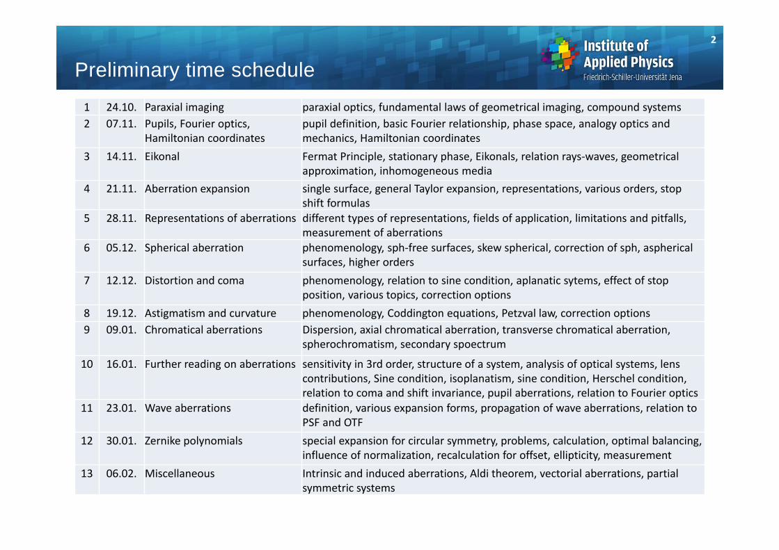
Preliminary time schedule
1 24.10. Paraxial imaging paraxial optics, fundamental laws of geometrical imaging, compound systems2 07.11. Pupils, Fourier optics,
Hamiltonian coordinatespupil definition, basic Fourier relationship, phase space, analogy optics and mechanics, Hamiltonian coordinates
3 14.11. Eikonal Fermat Principle, stationary phase, Eikonals, relation rays‐waves, geometrical approximation, inhomogeneous media
4 21.11. Aberration expansion single surface, general Taylor expansion, representations, various orders, stop shift formulas
5 28.11. Representations of aberrations different types of representations, fields of application, limitations and pitfalls, measurement of aberrations
6 05.12. Spherical aberration phenomenology, sph‐free surfaces, skew spherical, correction of sph, asphericalsurfaces, higher orders
7 12.12. Distortion and coma phenomenology, relation to sine condition, aplanatic sytems, effect of stop position, various topics, correction options
8 19.12. Astigmatism and curvature phenomenology, Coddington equations, Petzval law, correction options9 09.01. Chromatical aberrations Dispersion, axial chromatical aberration, transverse chromatical aberration,
spherochromatism, secondary spoectrum
10 16.01. Further reading on aberrations sensitivity in 3rd order, structure of a system, analysis of optical systems, lens contributions, Sine condition, isoplanatism, sine condition, Herschel condition, relation to coma and shift invariance, pupil aberrations, relation to Fourier optics
11 23.01. Wave aberrations definition, various expansion forms, propagation of wave aberrations, relation to PSF and OTF
12 30.01. Zernike polynomials special expansion for circular symmetry, problems, calculation, optimal balancing,influence of normalization, recalculation for offset, ellipticity, measurement
13 06.02. Miscellaneous Intrinsic and induced aberrations, Aldi theorem, vectorial aberrations, partial symmetric systems
1. Geometrical astigmatism
2. Point spread function for astigmatism
3. Field curvature
4. Petzval theorem
5. Correcting field curvature
6. Examples
3
Contents
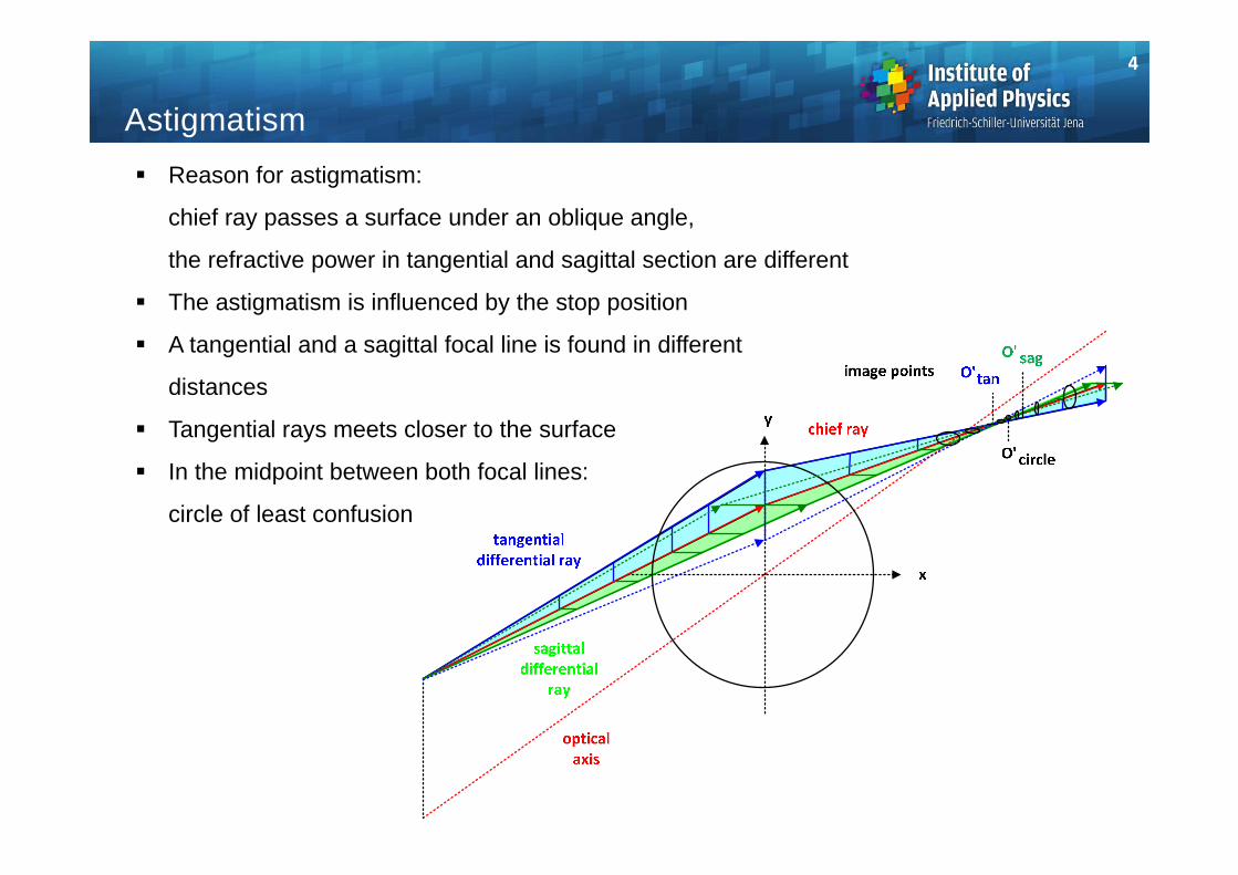
Reason for astigmatism:
chief ray passes a surface under an oblique angle,
the refractive power in tangential and sagittal section are different
The astigmatism is influenced by the stop position
A tangential and a sagittal focal line is found in different
distances
Tangential rays meets closer to the surface
In the midpoint between both focal lines:
circle of least confusion
Astigmatism
4
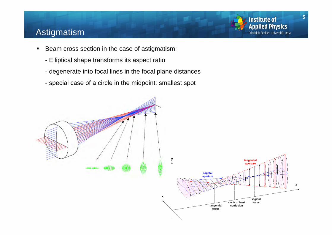
Beam cross section in the case of astigmatism:
- Elliptical shape transforms its aspect ratio
- degenerate into focal lines in the focal plane distances
- special case of a circle in the midpoint: smallest spot
y
x
z
tangentialfocus
sagittalfocuscircle of least
confusion
tangentialaperture
sagittalaperture
Astigmatism
5
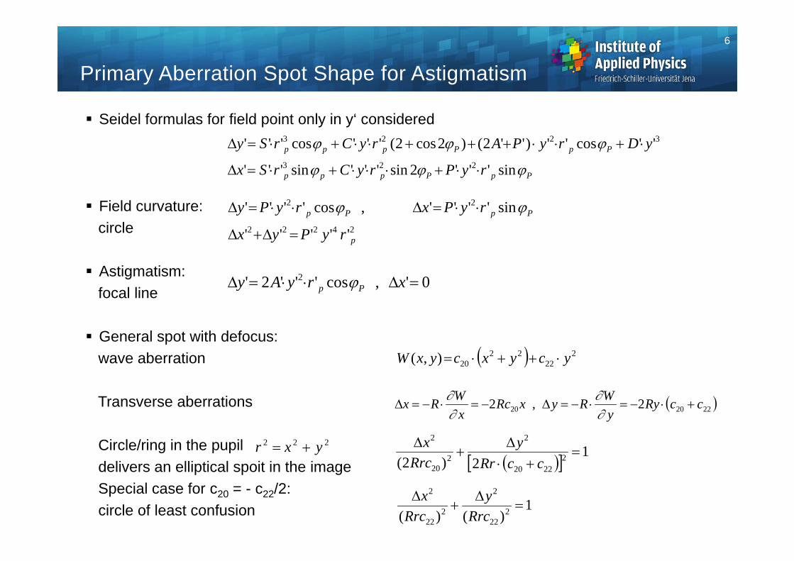
Primary Aberration Spot Shape for Astigmatism
Seidel formulas for field point only in y‘ considered
Field curvature:circle
Astigmatism:focal line
General spot with defocus:wave aberration
Transverse aberrations
Circle/ring in the pupil delivers an elliptical spoit in the imageSpecial case for c20 = - c22/2:circle of least confusion
PpPppp
PpPppp
ryPryCrSx
yDryPAryCrSy
sin'''2sin'''sin'''
''cos'')''2()2cos2('''cos'''223
3223
0',cos'''2' 2 xryAy Pp
24222
22
'''''
sin'''',cos''''
p
PpPp
ryPyx
ryPxryPy
222
2220),( ycyxcyxW
222020 2,2 ccRyy
WRyxRcx
WRx
r x y2 2 2 1
2)2( 22220
2
220
2
ccRr
yRrc
x
1)()( 2
22
2
222
2
Rrcy
Rrcx
6

At sagittal focus Defocus only in tangential cross section
Astigmatism
Wave aberrationtangential sagittal
22
Primary astigmatism at sagittal focus
Transverse ray aberration y x y
Pupil: y-section x-section x-section
0.01 mm 0.01 mm 0.01 mm
Modulation Transfer Function MTF MTF at paraxial focus MTF through focus for 100 cycles per mm
Geometrical spot through focus
0.02
mm
sagittal
tangential
tangential
sagittal
z/mm-0.04 0.040.0-0.02 0.02
1
0
0.5
0 100 200cyc/mm z/mm
1
0
0.5
0.040.0-0.04
Ref: H. Zügge
7
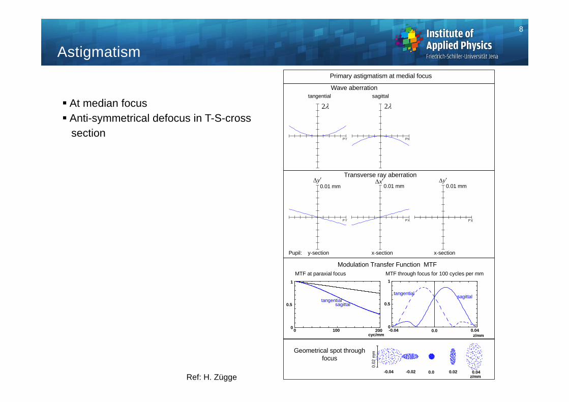
At median focus Anti-symmetrical defocus in T-S-cross
section
Astigmatism
Wave aberrationtangential sagittal
22
Primary astigmatism at medial focus
Transverse ray aberration y x y
Pupil: y-section x-section x-section
0.01 mm 0.01 mm 0.01 mm
Modulation Transfer Function MTF MTF at paraxial focus MTF through focus for 100 cycles per mm
sagittaltangentialtangential
sagittal
1
0
0.5
0 100 200cyc/mm z/mm
1
0
0.5
0.040.0-0.04
Geometrical spot through focus
0.02
mm
z/mm-0.04 0.040.0-0.02 0.02
Ref: H. Zügge
8
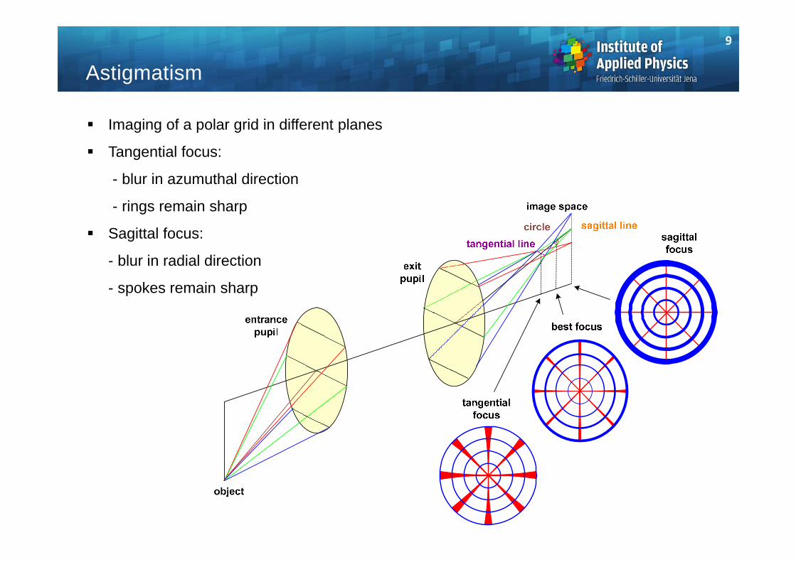
Imaging of a polar grid in different planes
Tangential focus:
- blur in azumuthal direction
- rings remain sharp
Sagittal focus:
- blur in radial direction
- spokes remain sharp
Astigmatism
9
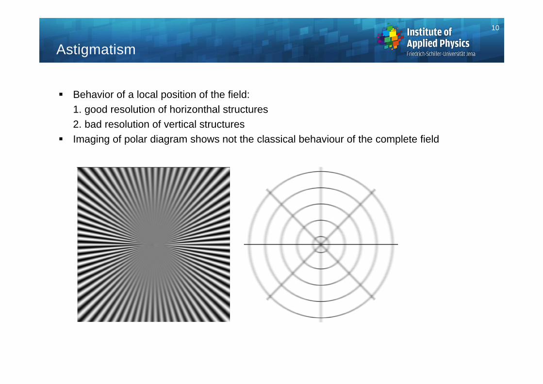
Astigmatism
Behavior of a local position of the field:1. good resolution of horizonthal structures2. bad resolution of vertical structures
Imaging of polar diagram shows not the classical behaviour of the complete field
10
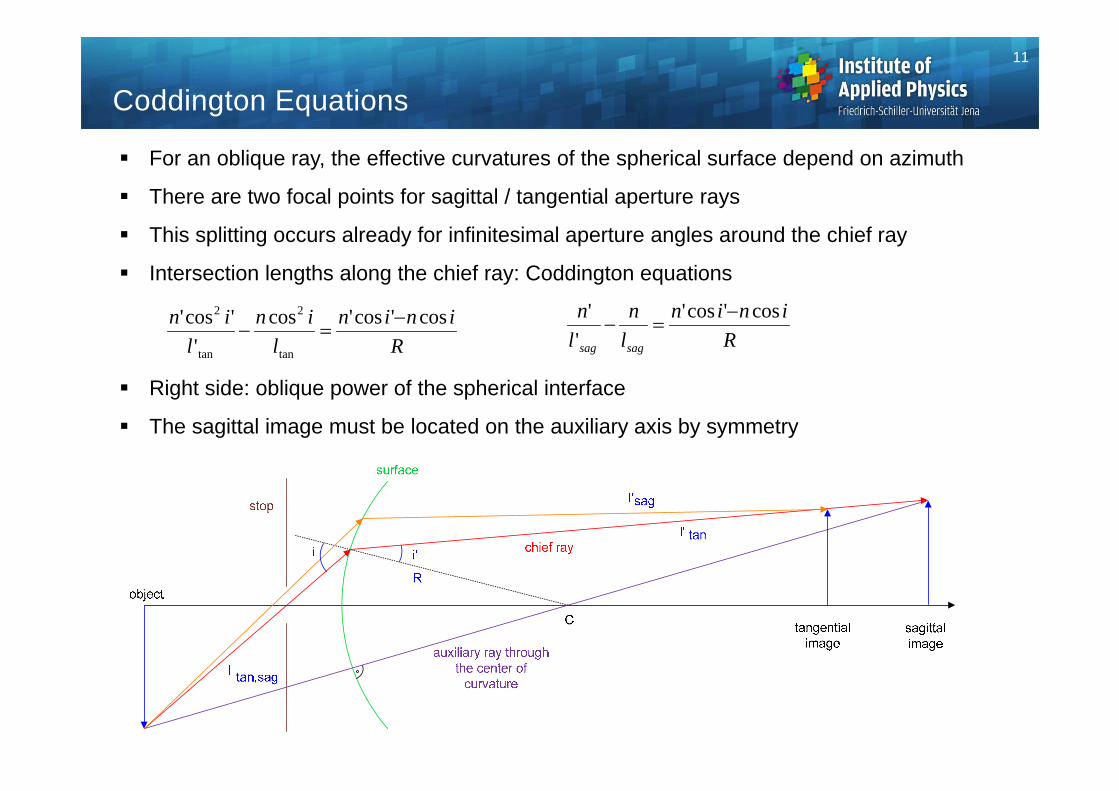
For an oblique ray, the effective curvatures of the spherical surface depend on azimuth
There are two focal points for sagittal / tangential aperture rays
This splitting occurs already for infinitesimal aperture angles around the chief ray
Intersection lengths along the chief ray: Coddington equations
Right side: oblique power of the spherical interface
The sagittal image must be located on the auxiliary axis by symmetry
Coddington Equations
Rinin
lin
lin cos'cos'cos
''cos'
tan
2
tan
2 R
ininln
ln
sagsag
cos'cos''
'
11
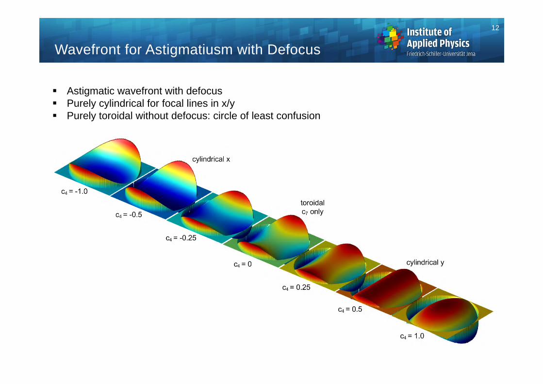
Wavefront for Astigmatiusm with Defocus
Astigmatic wavefront with defocus Purely cylindrical for focal lines in x/y Purely toroidal without defocus: circle of least confusion
12
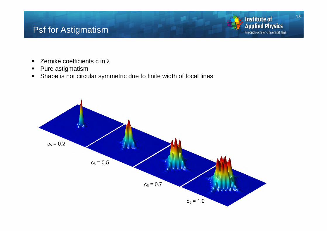
Psf for Astigmatism
Zernike coefficients c in Pure astigmatism Shape is not circular symmetric due to finite width of focal lines
13
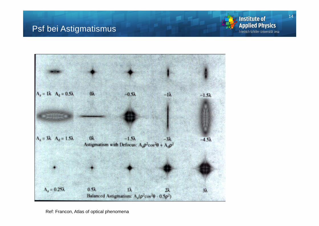
Psf bei Astigmatismus
Ref: Francon, Atlas of optical phenomena
14
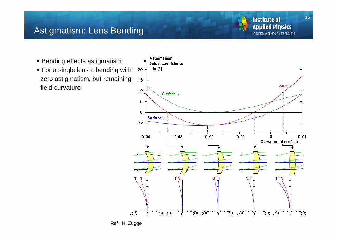
Bending effects astigmatism For a single lens 2 bending with
zero astigmatism, but remainingfield curvature
Astigmatism: Lens Bending
Ref : H. Zügge
15
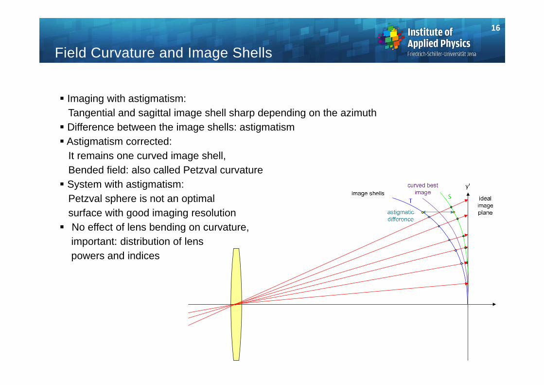
Field Curvature and Image Shells
Imaging with astigmatism:Tangential and sagittal image shell sharp depending on the azimuth Difference between the image shells: astigmatism Astigmatism corrected:
It remains one curved image shell,Bended field: also called Petzval curvature System with astigmatism:
Petzval sphere is not an optimalsurface with good imaging resolution No effect of lens bending on curvature,
important: distribution of lenspowers and indices
16
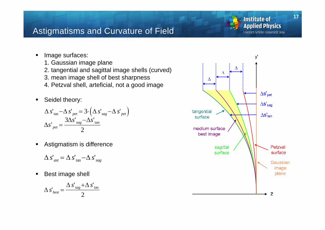
Astigmatisms and Curvature of Field
ss s
bestsag'' 'tan
2
s s s spet sag pet' ' ' 'tan 3
s s sast sag' ' 'tan
Image surfaces:1. Gaussian image plane2. tangential and sagittal image shells (curved)3. mean image shell of best sharpness4. Petzval shell, arteficial, not a good image
Seidel theory:
Astigmatism is difference
Best image shell
2''3
' tansss sag
pet
17
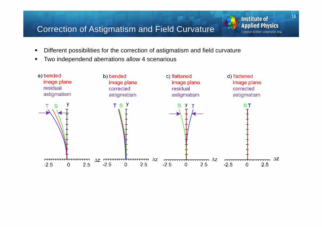
Correction of Astigmatism and Field Curvature
Different possibilities for the correction of astigmatism and field curvature Two independend aberrations allow 4 scenarious
18
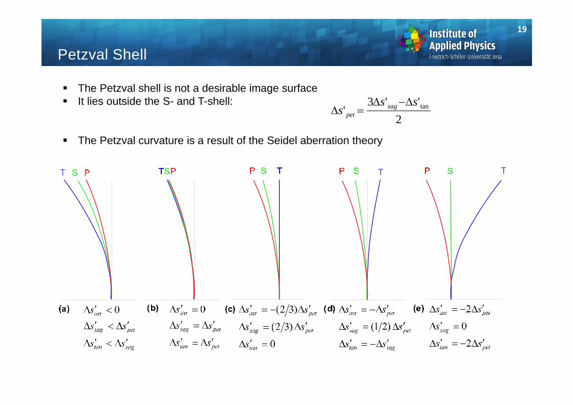
Petzval Shell
The Petzval shell is not a desirable image surface It lies outside the S- and T-shell:
The Petzval curvature is a result of the Seidel aberration theory
19
2''3
' tansss sag
pet
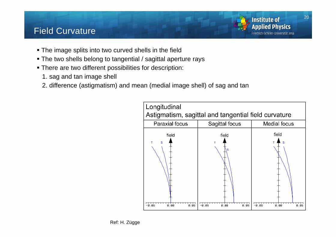
The image splits into two curved shells in the field The two shells belong to tangential / sagittal aperture rays There are two different possibilities for description:
1. sag and tan image shell2. difference (astigmatism) and mean (medial image shell) of sag and tan
Field Curvature
Ref: H. Zügge
20
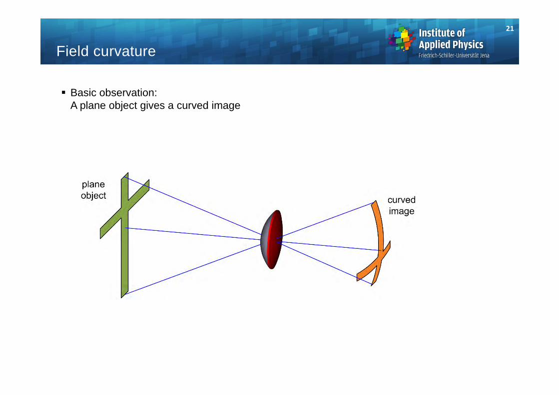
Basic observation:A plane object gives a curved image
21
Field curvature
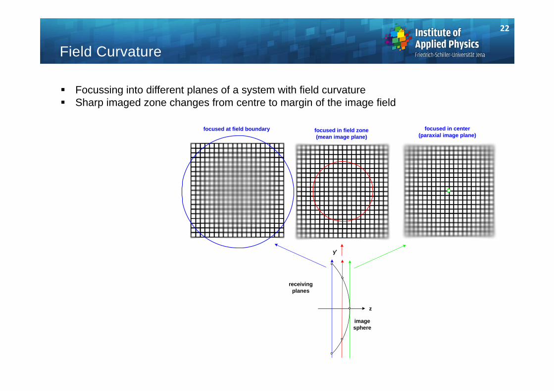
Focussing into different planes of a system with field curvature Sharp imaged zone changes from centre to margin of the image field
focused in center(paraxial image plane)
focused in field zone(mean image plane)
focused at field boundary
z
y'
receivingplanes
imagesphere
Field Curvature
22
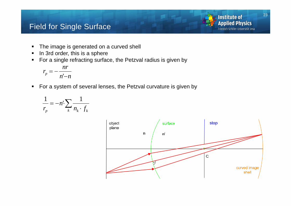
The image is generated on a curved shell In 3rd order, this is a sphere For a single refracting surface, the Petzval radius is given by
For a system of several lenses, the Petzval curvature is given by
Field for Single Surface
1 1r
nn fp k kk
'
r nrn np '
23
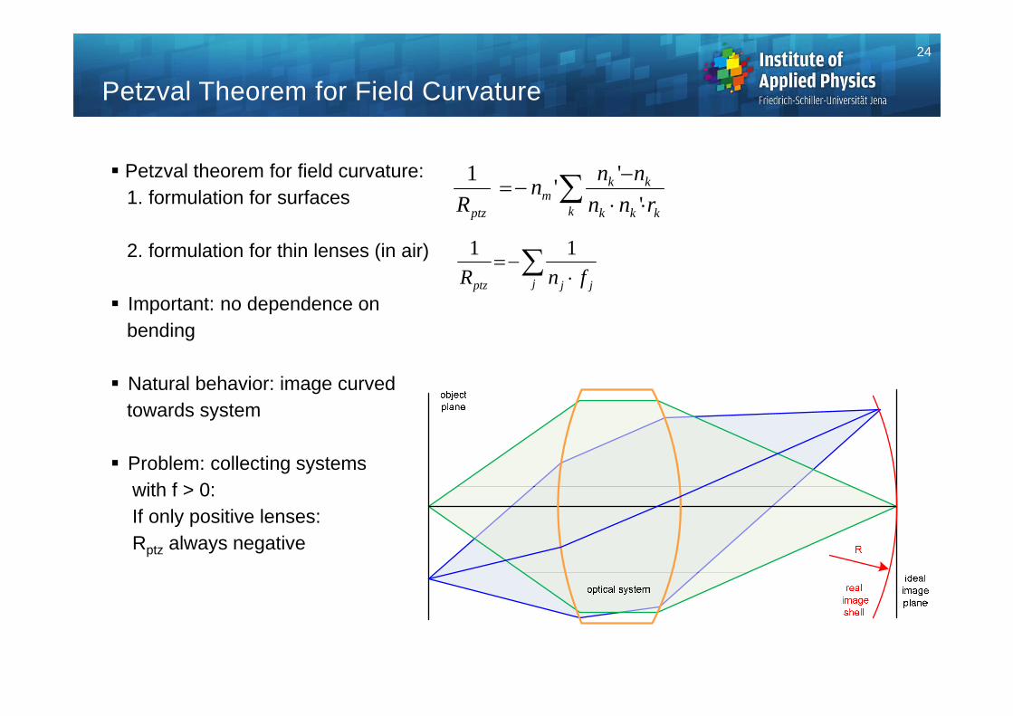
Petzval Theorem for Field Curvature
Petzval theorem for field curvature:1. formulation for surfaces
2. formulation for thin lenses (in air)
Important: no dependence on bending
Natural behavior: image curved towards system
Problem: collecting systems with f > 0:If only positive lenses: Rptz always negative
k kkk
kkm
ptz rnnnnn
R '''1
j jjptz fnR11
24
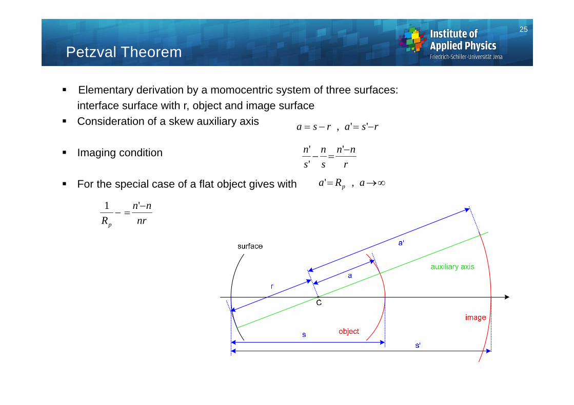
Petzval Theorem
Elementary derivation by a momocentric system of three surfaces:interface surface with r, object and image surface
Consideration of a skew auxiliary axis
Imaging condition
For the special case of a flat object gives with
rsarsa '',
rnn
sn
sn
'
''
nrnn
Rp
'1
aRa p ,'
25
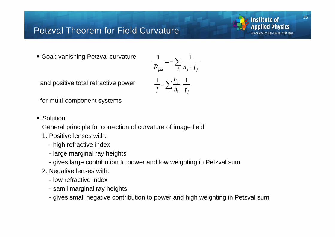
Petzval Theorem for Field Curvature
Goal: vanishing Petzval curvature
and positive total refractive power
for multi-component systems
Solution:General principle for correction of curvature of image field:1. Positive lenses with:
- high refractive index- large marginal ray heights- gives large contribution to power and low weighting in Petzval sum
2. Negative lenses with: - low refractive index- samll marginal ray heights- gives small negative contribution to power and high weighting in Petzval sum
j jjptz fnR11
jj
j
fhh
f11
1
26
Flattening Meniscus Lenses
Possible lenses / lens groups for correcting field curvature Interesting candidates: thick meniscus shaped lenses
1. Hoeghs mensicus: identical radii- Petzval sum zero- remaining positive refractive power
2. Concentric meniscus, - Petzval sum negative- weak negative focal length- refractive power for thickness d:
3. Thick meniscus without refractive powerRelation between radii
F n dnr r d
' ( )( )
1
1 1
r r d nn2 1
1
21
211'
'1rrd
nn
fnrnnnn
R k kkk
kk
ptz
r2
d
r1
2
2)1('rn
dnF
drr 12
drrndn
Rptz
11
)1(1
0)1(
)1(1
11
2
ndnrrndn
Rptz
27
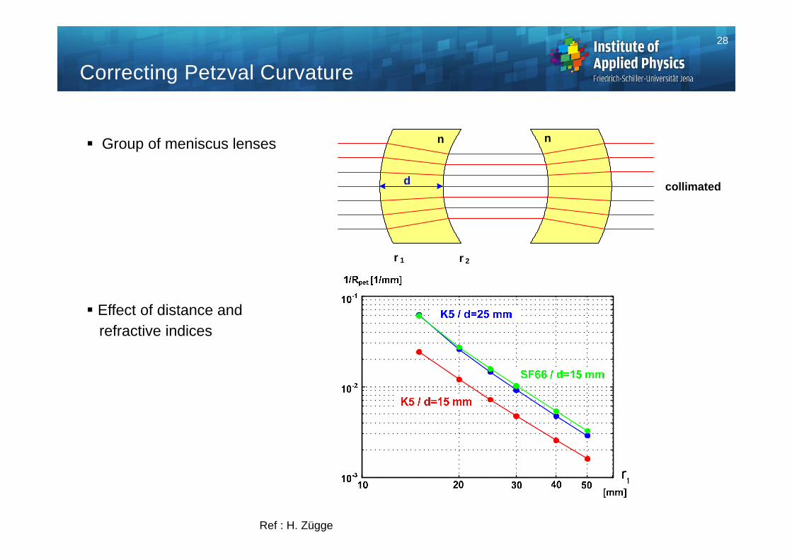
Group of meniscus lenses
Effect of distance and refractive indices
Correcting Petzval Curvature
r 2r 1
collimated
n n
d
Ref : H. Zügge
28
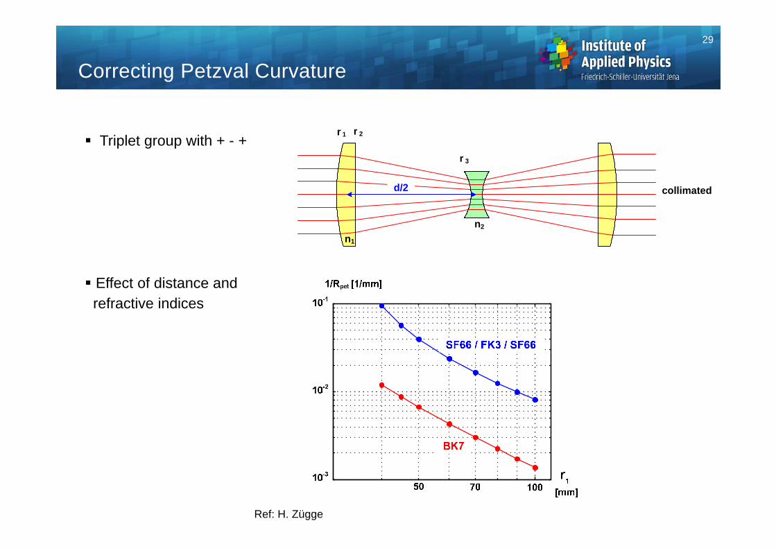
Triplet group with + - +
Effect of distance and refractive indices
Correcting Petzval Curvature
r 2r 1
collimated
n1
n2
r 3
d/2
Ref: H. Zügge
29
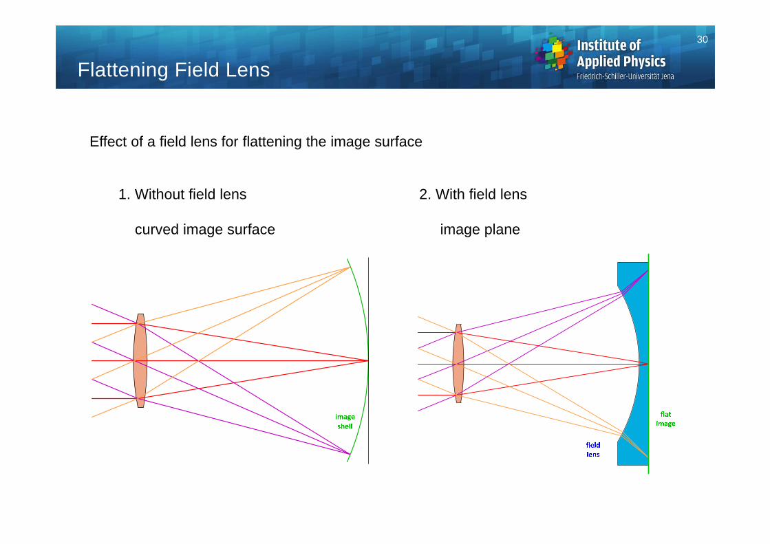
Effect of a field lens for flattening the image surface
1. Without field lens 2. With field lens
curved image surface image plane
Flattening Field Lens
30
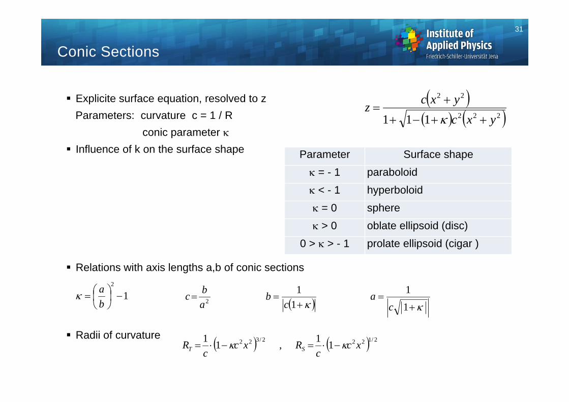
Conic Sections
222
22
111 yxcyxcz
12
ba
2abc
11
cb
1
1
ca
Explicite surface equation, resolved to zParameters: curvature c = 1 / R
conic parameter Influence of k on the surface shape
Relations with axis lengths a,b of conic sections
Radii of curvature
Parameter Surface shape = - 1 paraboloid < - 1 hyperboloid = 0 sphere > 0 oblate ellipsoid (disc)
0 > > - 1 prolate ellipsoid (cigar )
2/1222/322 11,11 xcc
Rxcc
R ST
31
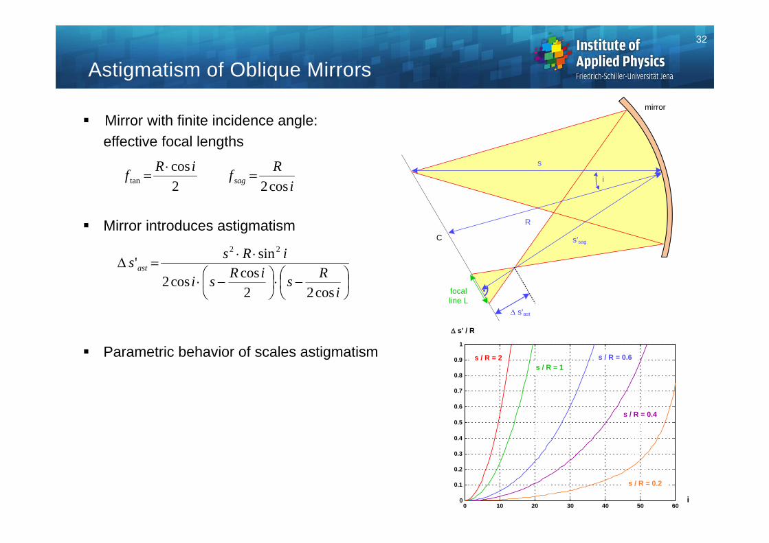
Astigmatism of Oblique Mirrors
Mirror with finite incidence angle:effective focal lengths
Mirror introduces astigmatism
Parametric behavior of scales astigmatism
2cos
taniRf
i
Rfsag cos2
iRsiRsi
iRss ast
cos22coscos2
sin'22
i0 10 20 30 40 50 60
0
0.1
0.2
0.3
0.4
0.5
0.6
0.7
0.8
0.9
1
s / R = 0.2
s / R = 0.4
s / R = 0.6s / R = 1
s / R = 2
s' / R
s'ast
R
focalline L
i
C
s
s'sag
mirror
32
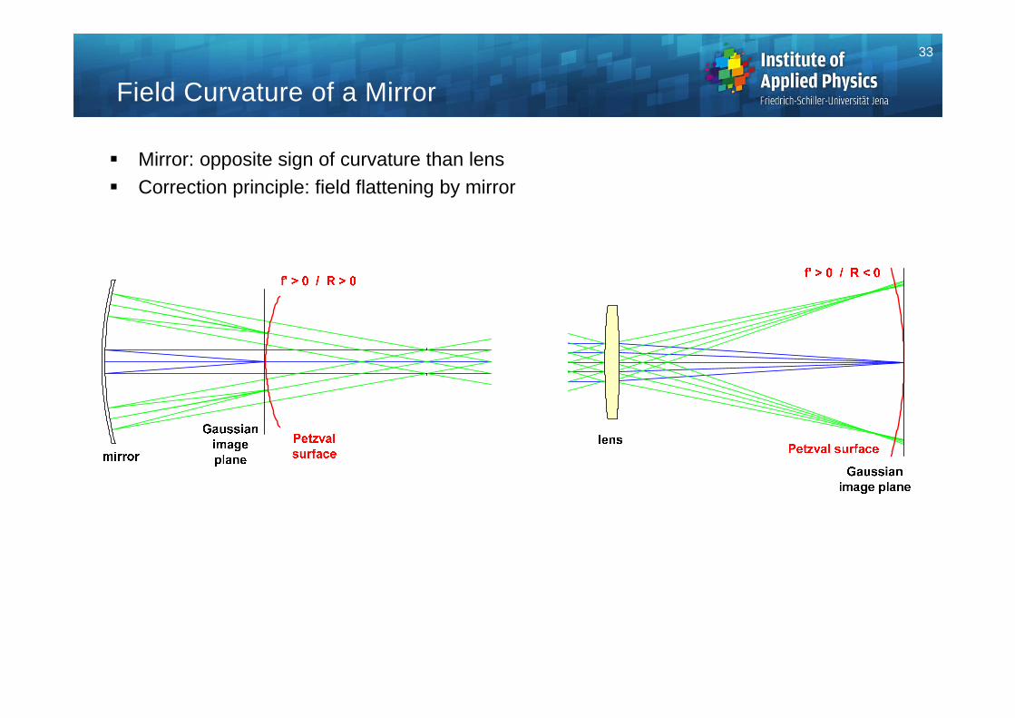
Field Curvature of a Mirror
Mirror: opposite sign of curvature than lens Correction principle: field flattening by mirror
33
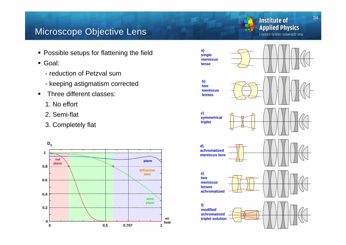
Microscope Objective Lens
Possible setups for flattening the field Goal:
- reduction of Petzval sum- keeping astigmatism corrected
Three different classes:1. No effort2. Semi-flat3. Completely flat
d)achromatizedmeniscus lens
a)singlemeniscuslense
e)twomeniscuslensesachromatized
b)twomeniscuslenses
c)symmetricaltriplet
f)modIfiedachromatizedtriplet solution
DS
rel.field
0 0.5 0.707 1
1
0.8
0.6
0.4
0.2
0
diffractionlimit
plane
semiplane
notplane
34
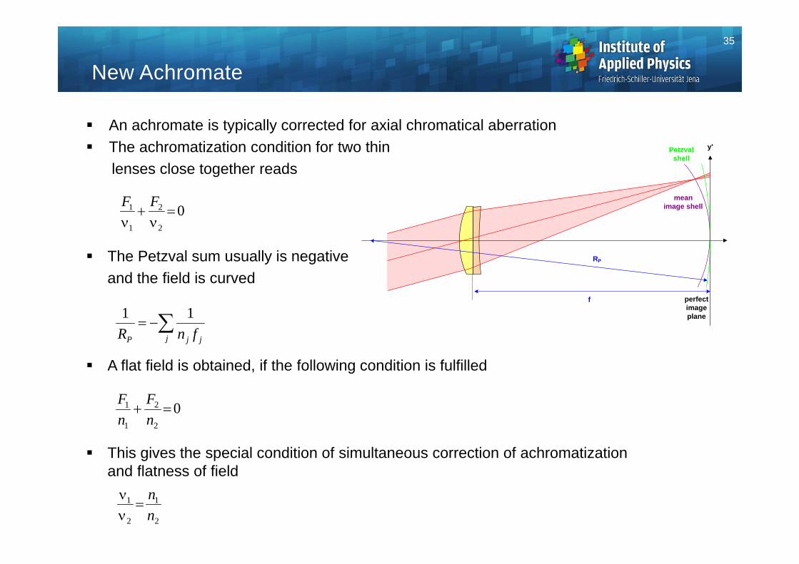
New Achromate
An achromate is typically corrected for axial chromatical aberration The achromatization condition for two thin
lenses close together reads
The Petzval sum usually is negative and the field is curved
A flat field is obtained, if the following condition is fulfilled
This gives the special condition of simultaneous correction of achromatization and flatness of field
perfect image plane
Petzvalshell
y'
f
RP
mean image shell0
2
2
1
1
FF
j jjP fnR
11
02
2
1
1 nF
nF
2
1
2
1
nn
35
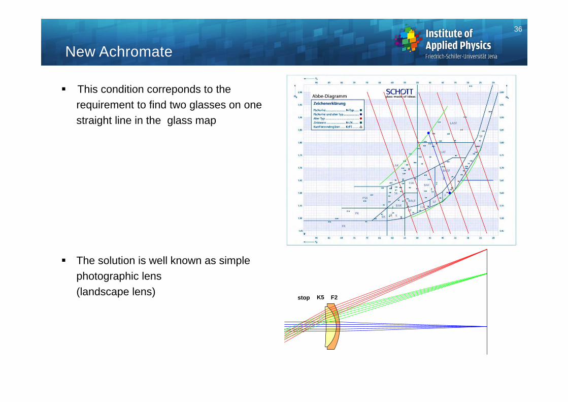
New Achromate
This condition correponds to the requirement to find two glasses on onestraight line in the glass map
The solution is well known as simplephotographic lens(landscape lens) K5 F2stop
36
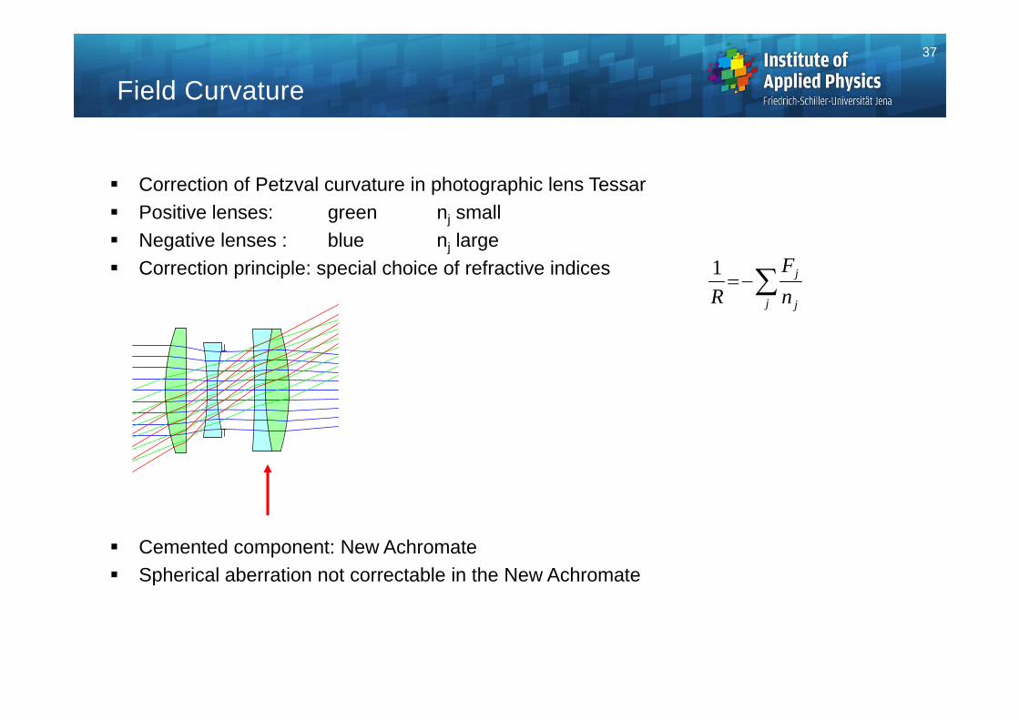
Field Curvature
Correction of Petzval curvature in photographic lens Tessar Positive lenses: green nj small Negative lenses : blue nj large Correction principle: special choice of refractive indices
Cemented component: New Achromate Spherical aberration not correctable in the New Achromate
j j
j
nF
R1
37
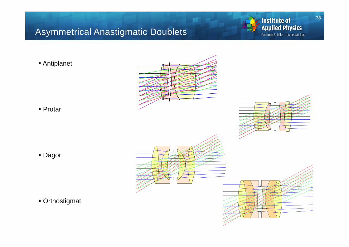
Antiplanet
Protar
Dagor
Orthostigmat
Asymmetrical Anastigmatic Doublets
38
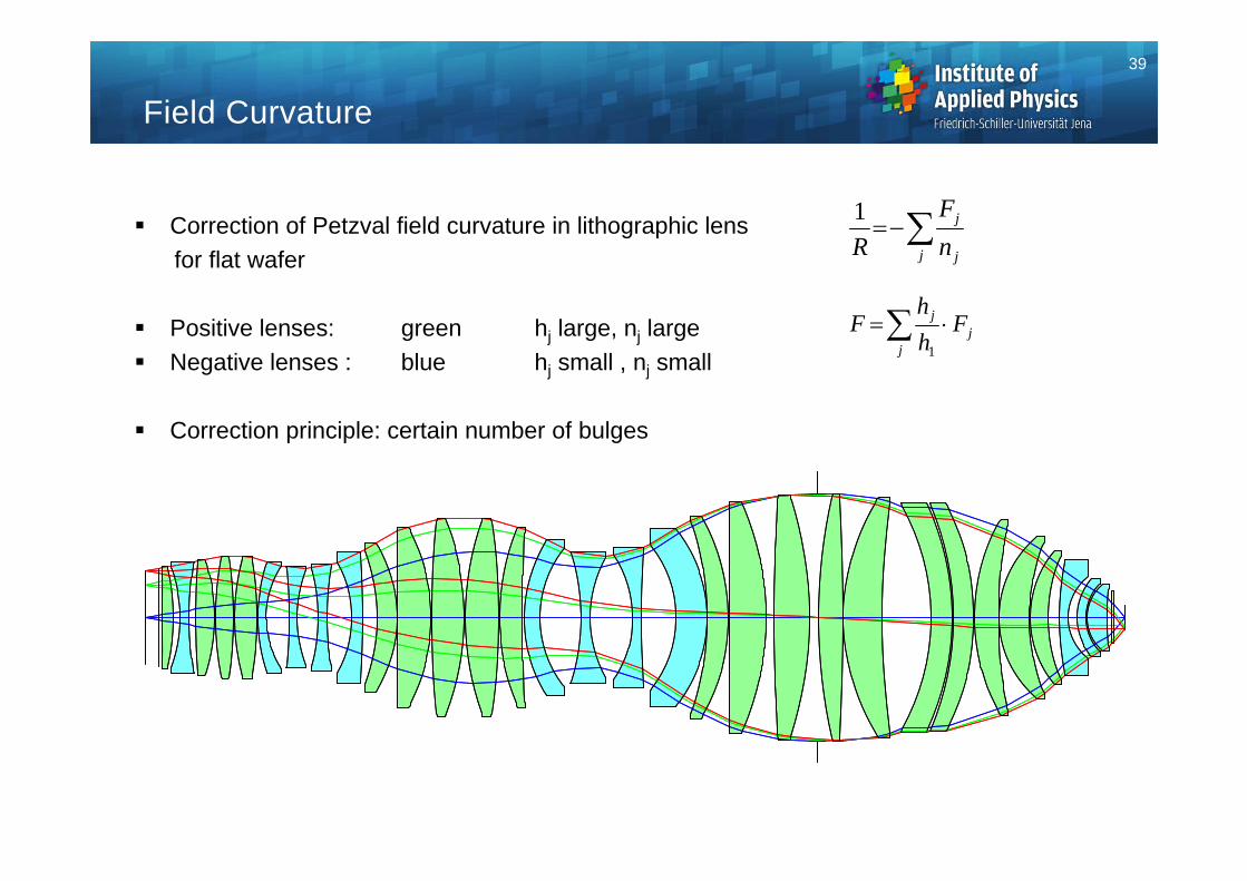
Field Curvature
Correction of Petzval field curvature in lithographic lensfor flat wafer
Positive lenses: green hj large, nj large Negative lenses : blue hj small , nj small
Correction principle: certain number of bulges
j j
j
nF
R1
jj
j Fhh
F 1
39
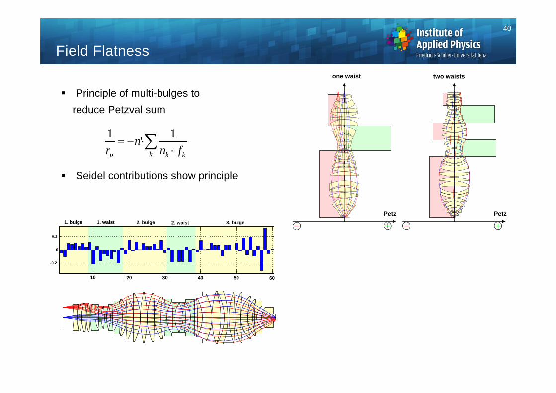
Field Flatness
Principle of multi-bulges toreduce Petzval sum
Seidel contributions show principle
-0.2
0
0.2
10 20 30 40 6050
1. bulge 2. bulge 3. bulge1. waist 2. waist
one waist two waists
Petz Petz
1 1r
nn fp k kk
'
40
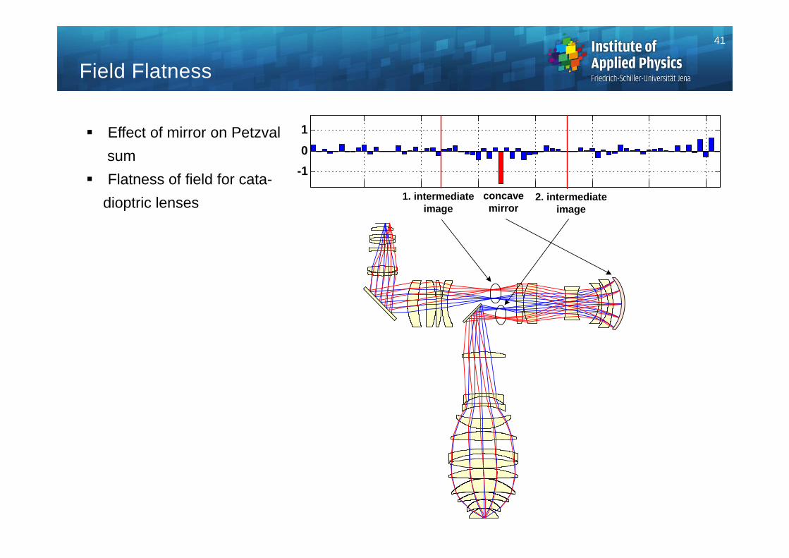
Field Flatness
Effect of mirror on Petzvalsum
Flatness of field for cata-dioptric lenses
-101
concavemirror
1. intermediateimage
2. intermediateimage
41
Field Curvature
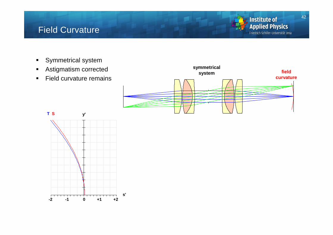
Symmetrical system Astigmatism corrected Field curvature remains
fieldcurvature
symmetricalsystem
s'
T S y'
-2 -1 0 +1 +2
42
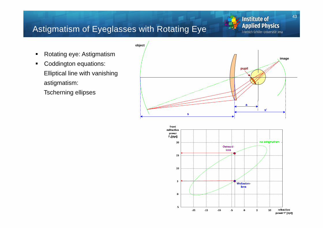
Astigmatism of Eyeglasses with Rotating Eye
Rotating eye: Astigmatism Coddington equations:
Elliptical line with vanishing astigmatism:Tscherning ellipses
a
object
s'
image
pupil
s
43
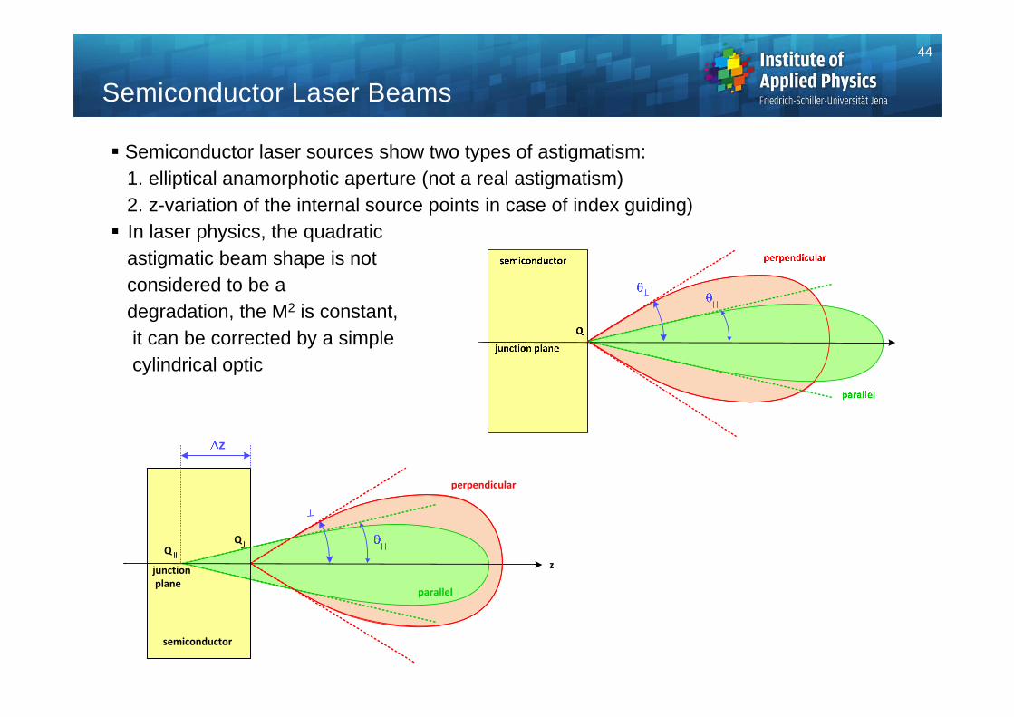
Semiconductor laser sources show two types of astigmatism:1. elliptical anamorphotic aperture (not a real astigmatism)2. z-variation of the internal source points in case of index guiding) In laser physics, the quadratic
astigmatic beam shape is not considered to be adegradation, the M2 is constant, it can be corrected by a simple cylindrical optic
Semiconductor Laser Beams
z
z
Q
parallel
Q
perpendicular
semiconductor
junctionplane
44
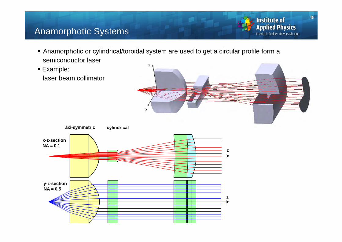
Anamorphotic or cylindrical/toroidal system are used to get a circular profile form a semiconductor laser Example:
laser beam collimator
Anamorphotic Systems
x
y
x-z-sectionNA = 0.1
y-z-sectionNA = 0.5
z
cylindricalaxi-symmetric
z
45
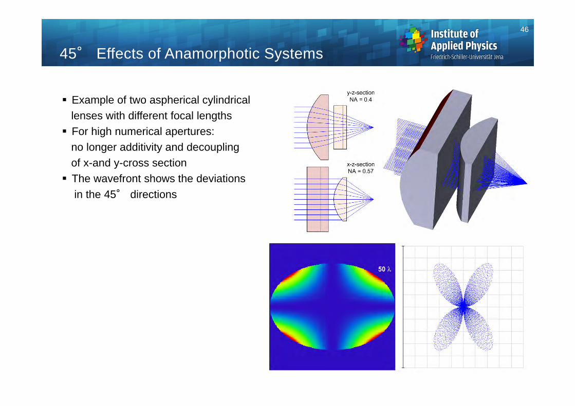
45° Effects of Anamorphotic Systems
Example of two aspherical cylindricallenses with different focal lengths For high numerical apertures:
no longer additivity and decouplingof x-and y-cross section The wavefront shows the deviations
in the 45° directions
46
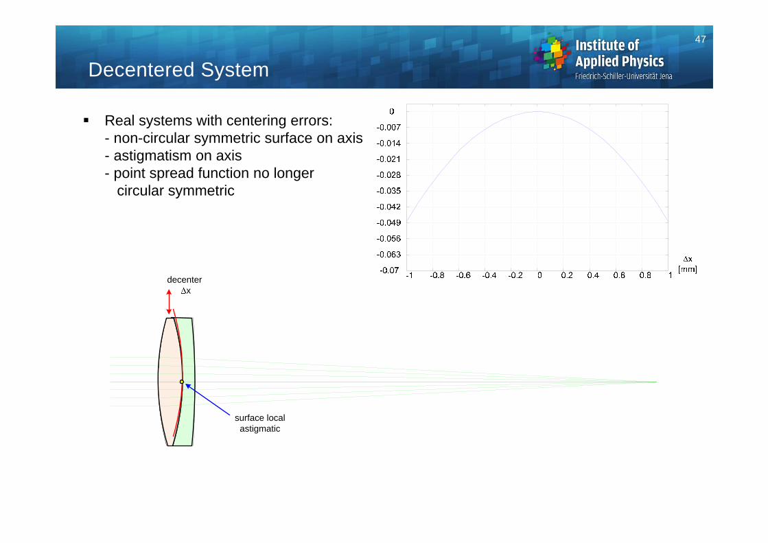
Decentered System
Real systems with centering errors:- non-circular symmetric surface on axis- astigmatism on axis- point spread function no longer
circular symmetric
decenterx
surface local astigmatic
47
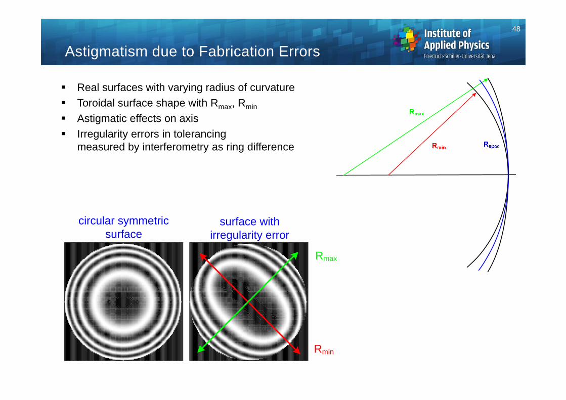
Astigmatism due to Fabrication Errors
Real surfaces with varying radius of curvature Toroidal surface shape with Rmax, Rmin
Astigmatic effects on axis Irregularity errors in tolerancing
measured by interferometry as ring difference
circular symmetric surface
surface with irregularity error
Rmin
Rmax
48
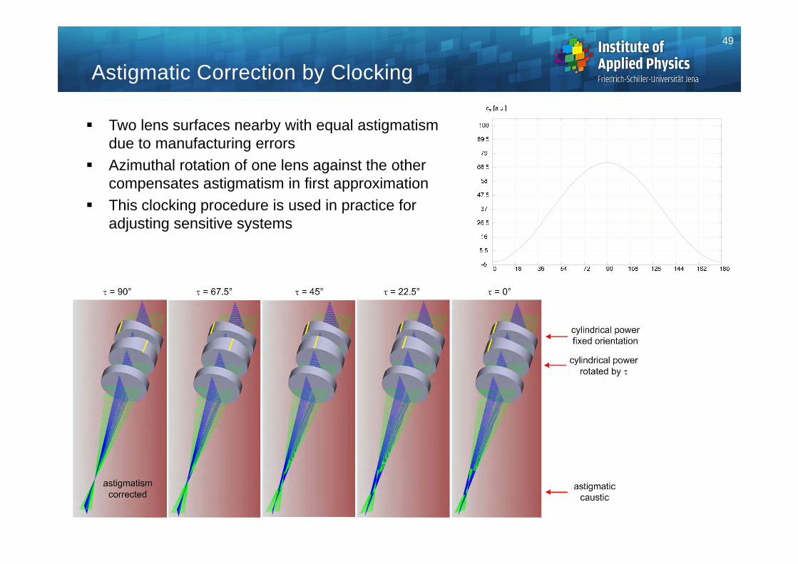
Astigmatic Correction by Clocking
Two lens surfaces nearby with equal astigmatismdue to manufacturing errors
Azimuthal rotation of one lens against the othercompensates astigmatism in first approximation
This clocking procedure is used in practice foradjusting sensitive systems
49
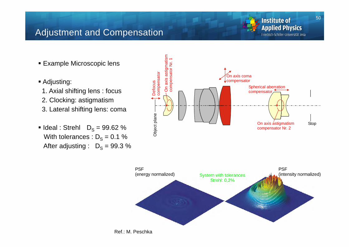
Example Microscopic lens
Adjusting:1. Axial shifting lens : focus2. Clocking: astigmatism3. Lateral shifting lens: coma
Ideal : Strehl DS = 99.62 %With tolerances : DS = 0.1 %After adjusting : DS = 99.3 %
Adjustment and Compensation
System with tolerancesStrehl: 0,2%
PSF (intensity normalized)
PSF(energy normalized)
Spherical aberrationcompensator
On axis comacompensator
Stop
Obj
ect p
lane
Def
ocus
com
pens
ator
On
axis
ast
igm
atis
mco
mpe
nsat
or N
r. 1
On axis astigmatismcompensator Nr. 2
Ref.: M. Peschka
50
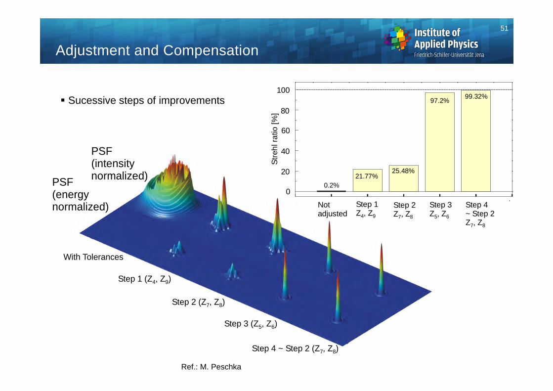
Sucessive steps of improvements
Adjustment and Compensation
PSF(intensitynormalized)
With Tolerances
Step 1 (Z , Z )4 9
Step 2 (Z , Z )7 8
Step 3 (Z , Z )5 6
Step 4 ~ Step 2 (Z , Z )7 8
PSF(energynormalized) Not
adjusted
0.2%21.77%
25.48%
97.2% 99.32%
Stre
hl ra
tio [%
]
0
20
40
60
80
100
Step 1Z , Z4 9
Step 2Z , Z7 8
Step 3Z , Z5 6
Step 4~ Step 2Z , Z7 8
Ref.: M. Peschka
51