Images as Sets of Locally Weighted Features✩

Teofilo de Camposa, Gabriela Csurkab, Florent Perronninb

aCVSSP, University of Surrey

Guildford, GU2 7XH, UKbXerox Research Centre Europe

6, chemin de Maupertuis, 38240 Meylan, France

Abstract

This paper presents a generic framework in which images are modelled asorder-less sets of weighted visual features. Each visual feature is associatedwith a weight factor that may inform its relevance. This framework can beapplied to various bag-of-features approaches such as the bag-of-visual-wordor the Fisher kernel representations. We suggest that if dense sampling isused, different schemes to weight local features can be evaluated, leadingto results that are often better than the combination of multiple samplingschemes, at a much lower computational cost, because the features are ex-tracted only once. This allows our framework to be a test-bed for saliencyestimation methods in image categorisation tasks. We explored two mainpossibilities for the estimation of local feature relevance. The first one isbased on the use of saliency maps obtained from human feedback, either bygaze tracking or by mouse clicks. The method is able to profit from suchmaps, leading to a significant improvement in categorisation performance.The second possibility is based on automatic saliency estimation methods,including Itti&Koch’s method and SIFT’s DoG. We evaluated the proposedframework and saliency estimation methods using an in house dataset andthe PASCAL VOC 2008/2007 dataset, showing that some of the saliencyestimation methods lead to a significant performance improvement in com-

✩This paper is available from http://dx.doi.org/10.1016/j.cviu.2011.07.011

The research leading to these results has received funding from the European Community’sSeventh Framework Programme (FP7/2007–2013) under grant agreement n◦ 216529, Per-sonal Information Navigator Adapting Through Viewing, PinView. TdC was also sup-ported by the EPSRC-UK grant EP/F069421/1 (ACASVA) while writing this paper.

∗Corresponding author: T. de Campos, t.decampos@st-annes.oxon.org

Preprint submitted to CVIU Submitted: November 27, 2009 Revised: May 24, 2011

Figure 1: The framework proposed and evaluated in this paper.

parison to the standard unweighted representation.

Keywords: bag-of-visual-words, image categorisation, saliency estimation

1. Introduction

The bags of features approach (BoF) has become a gold-standard methodfor categorisation and retrieval of generic images, such as photos taken bynon-professional photographers. This is mostly due to its high degree of in-variance, but this comes at the expense of some loss in discrimination power.To deal with that, Uijlings et al. [54] have assessed the idea of providingobject location information in the form of bounding boxes to restrict wherefeatures are extracted. They conclude that “object localisation, if done suf-ficiently precise, helps considerably in the recognition of objects”. A keyproblem with this is how to cope with the inaccuracy of object detectors andtheir high computational cost. Without attempting to produce better objectdetectors, we investigate how to improve image categorisation systems byusing some loose knowledge of the relevance of each image region.

BoF-based methods follow this basic pipeline: (i) feature detection, (ii)low-level feature extraction, (iii) combination of features to build a global(or regional) image representation, i.e. a signature, and (iv) classification.In this paper, we explore the use of relevance weights, obtained from visualsaliency estimation methods, to enhance the image representation (iii).

2

The design of visual saliency models have been a topic of much interest incomputer vision. They can be used to drive feature detection and to estimateregions of interest. Many of these methods are inspired by biological visionmodels which aim at estimating which parts of images attract visual atten-tion. In terms of their implementation in computer systems, these methodsfall into two main categories: those that give a number of relevant punctualpositions, known as interest- or key-point detectors, and those that give amore continuous map of relevance, such as saliency maps.

Interest point detectors have proven useful to obtain reliable correspon-dences for matching (e.g. [26, 31, 33, 34]). They have also been extensivelyevaluated as a means to sparsely select positions to extract image featuresfor categorisation or object recognition [46, 8, 64]. However, it has beenshown that strategies based on random sampling (e.g. [56]) provide betterperformance (both in accuracy and speed) than interest points [37]. Sincethen, dense sampling has become more popular1. One of the reasons is thatinterest point detectors may disregard background regions of the image thatcarry important category information, such as the sky for airplane images.Another reason is their reduced robustness with respect to variations in-troduced, for instance, by shadows. However, interest-point detectors cancomplement dense feature extraction, as done in the top performing methodof the PASCAL challenge in 2007 (INRIA [12]), 2008 (UvA&Surrey [13])and 2010 (NUSPSL [14]). In these works, sampling and feature extractionmethods are treated as different channels and the channels are fused in amultiple kernel learning framework. The downside of these approaches are:(i) additional sampling strategies increase the computational cost, (ii) ad-ditional kernel computations are expensive and (iii) the complexity of theclassification system also increases, as discussed in Section 5.3.

While interest points are sparse corner (e.g. Harris) or blob (e.g. Lapa-cian) detectors, saliency maps can carry higher level information and pro-vide richer information about the relevance of features throughout an image.Most of the methods were designed to model visual attention and have beenevaluated by their congruence with fixation data obtained from experimentswith eye gaze trackers (e.g. [17, 38, 29, 53, 20, 3, 61]). Their use for ob-

1In this paper, by dense sampling we mean that features are extracted at patches ofmultiple scales located on a regular grid, covering the whole image, with an overlap of atleast 50% between each patch.

3

ject recognition or image categorisation is more recent. In [35] and [39],saliency maps are used to control the sampling density for feature extrac-tion. A classification-based method is used in [35] while in [39] a low-levelcontext-based method is proposed. Alternatively, saliency maps can be usedas foreground detection methods to provide regions of interest (ROI) for clas-sification [43]. It has been shown that extracting image features only aroundROIs or on segmented foreground gives better results than sampling featuresuniformly through the image [63, 36, 64, 55]. The disadvantage is that suchmethods heavily rely on foreground detection and they may miss importantcontext information from the background.

In this paper, in contrast to using saliency to determine the location ofimage features or their sampling density, we use this information to assignweights to image features. The main idea (summarised in Figure 1) is toestimate for each image a saliency map. The maps are used to locally weightthe features, which can be extracted on a dense grid. The weights are takeninto consideration when the feature statistics are cumulated to represent theimage in a bag-of-features approach. We evaluated this method with a GMM-based soft assignment bag-of-visual words method (BoW) [16] and with aFisher kernel (FK) representation. The obtained vectorial representation canbe used for categorisation, clustering or retrieval. In this paper, we evaluateit for image categorisation.2

The benefits of this approach are multiple. First, it can handle keypoint-based sampling and continuous saliency maps in the same framework: in thefirst case the maps are sparse and sharply peaked, while in the latter casesthey are smooth. Secondly, if soft weighting is used, this method highlightsthe foreground without disregarding the background (as opposed to ROI-based methods3). Finally, by using dense sampling, the feature extractionprocess only happens once, regardless of how many different saliency mapsare used to weight the features. Thus, saliency maps generated from different

2The core idea presented here was first described by the authors in a project report [4].The use of fixed maps to weight features was then evaluated in [58] as a way to introducelocality information in a bag-of-visual-words framework. In the present paper, the saliencymaps are computed individually, for each image, depending on its contents.

3Our representation can be seen as a generalisation of ROI-based methods becauseit becomes equivalent to such methods if binary saliency maps are used. But we haveobserved that this under-performs the use of smoother maps which incorporate informationof the background and account for imprecisions of bounding boxes.

4

sources can be used in the same framework. For instance, one can use gazetracking data, supervised foreground probability maps, maps generated fromvisual attention models, interest point detectors, object location priors etc.In addition, the image can be filtered globally in the computation of featureextraction, which is more efficient than processing patches individually, asit happens in the original implementations of keypoint-based methods. Thisallows the proposed framework to be used as a test-bed for saliency estimationmethods.

The rest of this paper is organised as follows. The next section describeshow we incorporate relevance weights in the image representations. Sec-tion 3 presents methods to estimate saliency maps, starting with methodsthat use human feedback, followed by automatic bottom-up and top-downmethods. The top-down methods described here share some componentswith the global image description methods, because they are also based onbag-of-features. The two datasets used in our experiments are described inSection 4, and the experiments are in Section 5. The paper is concluded inSection 6.

2. Bag of Weighted Features

Bag of Features (BoF) is a family of methods in which an image is rep-resented as an order-less set (i.e. a bag) of local feature vectors X = {xt, t =1, · · · , T}. To obtain a global representation of an image, most of the BoFmethods make use of an intermediate representation generally referred to asthe visual vocabulary [46, 8] whose parameters will be denoted λ in the fol-lowing. Using the visual vocabulary, each local feature xt is transformed intoa higher-level statistic gt and the global image representation is the averageof these statistics:

u(X, λ) =1

T

T∑

t=1

gt, (1)

i.e., images are represented using an average pooling of patch-level statis-tics [2].

The general idea of our method is to associate an individual weight factorψt to each feature vector xt which leads to the following global representation

5

of locally weighted statistics4:

uw(X, λ) =1

T

T∑

t=1

ψtgt. (2)

In this section, we describe how to integrate these weights in two represen-tations based on the average pooling framework. The computation of weightfactors is the subject of Section 3.

As mentioned above, the BoF methods use an intermediate representa-tion, the visual vocabulary. Most of the BoF methods use vector quantisa-tion of the image features to build the vocabulary and compute the code-word counts over local areas c.f. [8, 46]. The literature shows that betterperformances are obtained with pooling continuous sparse codes by usingsoft voting mechanisms [19] or, in a more principled fashion, a generativemodel [16, 40]. In this case, the visual vocabulary is a probability densityfunction (pdf) – denoted p – which models the emission of the low-leveldescriptors in the image.

In our experiments, we model the visual vocabulary as a Gaussian mixturemodel (GMM) where each Gaussian corresponds to a visual word [16]. Inthe case of a GMM, we have λ = {wi,µi,Σi, i = 1, · · · , N} where wi, µi

and Σi denote respectively the weight, mean vector and covariance matrixof Gaussian i and where N denotes the number of Gaussians. Let pi be thecomponent i of the GMM so that we have p(x) =

∑N

i=1wipi(x). We nowconsider two special cases of vocabulary-based average pooling approaches:the well-known GMM-based bag-of-visual-words (BoW) and the Fisher kernel(FK).

BoW: It consists in counting the number of occurrences of visual wordsin the image (soft occurrences in a probabilistic setting). Let γi(xt) be theposterior probability that the low-level descriptor xt is assigned to Gaussiani. This quantity can be computed using Bayes formula:

γi(xt) , p(i|xt, λ) =wipi(xt|λ)

∑N

j=1wjpj(xt|λ). (3)

Let γ(xt) be the N -dimensional vector [γ1(xt), · · · , γN(xt)]. In GMM-basedBoW we have gt = γ(xt).

5

4We chose the convention∑T

t=1ψt = T .

5In hard voting BoW [8], γi(xt) = 1[i = argminj(d(xt,xi))], where 1[·] is an indicator

6

FK: The set of feature vectors X is characterised by the following gradientvector [41]:

u(X, λ) =1

T∇λ log p(X|λ). (4)

This gradient vector describes in which direction the parameters of the genericmodel p should be modified to best fit the data. The vector u(X, λ) is subse-quently whitened using the normalisation technique described in [41]. Usingan independence assumption, we have:

u(X, λ) =1

T

T∑

t=1

∇λ log p(xt|λ) (5)

and therefore gt = ∇λ log p(xt|λ). For simplicity, the covariance matrices areassumed diagonal and we use the notation σ

2i = diag(Σi). Straightforward

differentiations provide the following formulae:

∂ log p(xt|λ)

∂µdi

= γi(xt)

[

xdt − µdt

(σdi )2

]

, (6)

∂ log p(xt|λ)

∂σdi

= γi(xt)

[

(xdt − µdi )

2

(σdi )3

−1

σdi

]

. (7)

The superscript d in (6) and (7) denotes the d-th dimension of a vector. Thegradient vector is just a concatenation of the partial derivatives with respectto the parameters µd

i and σdi of each Gaussian i, for i = 1, · · · , N :

gt =

[

· · · ,∂ log p(xt|λ)

∂µdi

,∂ log p(xt|λ)

∂σdi

, · · ·

]

(8)

and the global image representation is computed by u(X, λ) = 1T

∑T

t gt. Wedo not consider the partial derivatives with respect to the weight parame-ters (∂ log p(xt|λ)/∂wi) as it was shown in [41] to have little impact on thecategorisation accuracy. We note that computing the weighted global repre-sentation using (2) is equivalent to replacing log p(xt|λ) by ψt log p(xt|λ) in(5). This means that the weighted versions of FK, BoW or any other averagepooling method can be obtained in the same way (uw(X, λ) = 1

T

∑T

t ψtgt),c.f. (2), except that gt statistics are computed using different assumptions.

function, d is a distance measure and xi is the centroid of word i in the vocabulary. Thisis equivalent to average-pooling binary features [2].

7

It was shown in [41] that the FK generalises the BoW. Similarly, theweighted FK generalises the weighted BoW.

In [44], we show that FK “can be understood as the sample estimateof a class-conditional expectation” and that there are two main sources ofvariance in this estimation process: the fact that it is based on samplingfrom a finite pool of descriptors and the variance between images. We thenshow that the proposed local weighting mechanism can increase the classseparability by compensating the inter image variance, even if this weightingmechanism is applied in a class-independent fashion.

Jegou et al. [24] investigated the burstiness of visual elements, i.e., theeffect that repetitive textures such as brick walls have in bag-of-patches ap-proaches. Features with high burstiness lead to peaks in the global pool-basedsignature, but these features may not be relevant to categorise an image orretrieve images with similar contents. This effect is particularly more dam-aging in keypoint-based approaches if the repetitive patterns present highfrequency components. Jegou et al. proposed heuristics based on the idfstrategy. We advocate that by using saliency maps to weight local statistics,regions with repeated patterns (i.e. with lower saliency) will receive lowerweights. This automatically compensates for the burstiness effect6.

3. Weighting Features using Saliency Maps

In order to determine the relevance ψt of a feature, we use visual saliencymaps. Saliency maps are topographically arranged maps that represent visualsaliency of a scene [18]. In this paper we use this term more loosely todenominate bitmaps in which an importance value is assigned to each pixel.Similar maps have also been referred to as “heat maps” in the literature.

Given the saliency map of an image, different strategies can be used tocompute the relevance weight ψt of xt, a feature vector that describes patch t.For instance, one can use the saliency value at the centre of the patch. Otherpossibilities are the mean and the maximum value of the map at the area ofthe patch. We have compared these three strategies (mean, maximum andcentral value) in experiments with a dataset using saliency maps computedfrom gaze data (see Figure 14 and later discussion of results).

6Although top-down saliency maps are not designed to penalise regions with repeatedpatterns, they only enhance those which are relevant for an object class, i.e., a repeatedpattern may be highlighted only if that pattern characterises a class.

8

We have also explored class-dependent saliency maps, i.e., maps whichhighlight areas of high likelihood of classes of objects. In this case, C mapscan be associated to each image, where C is the number of classes considered.This gives class dependent weight factors ψc

t for each feature xt. Accordingly,we obtain a different weighted representation per class. In this case uw(X, λ)is replaced by

ucw(X, λ) =

1

T

T∑

t=1

ψctgt , (9)

so each image is represented by C vectors. In a one-versus-all classificationscheme, each classifier takes the corresponding class-dependent vector as itsinput, both at training and testing.

We consider two main approaches to compute saliency maps: using datagathered from users and fully automatic methods. These methods are de-scribed in Sections 3.1 and 3.2, respectively.

3.1. Using Feedback Provided by Humans

Most of the research in computer vision tries to avoid having humanin the loop, but many realistic applications require some level of humanfeedback such as image retrieval and image annotation. For instance, Winnet al. [63] use mouse clicks to indicate relevant objects or regions of interest.Image annotation is still done completely manually in most large commercialrepositories. The annotation work can be greatly facilitated if the systemautomatically suggest labels for images as the user visualises new images orclicks on their regions of interest.

Explicit feedback is acquired with the user’s intention, using some point-ing device. Additionally implicit feedback can seamlessly be obtained fromusers, without their explicit intention to indicate their interest. Since weare interested on visual attention, the best source of implicit feedback aregaze patterns, which can be captured with eye tracking systems. Such sys-tems are fast and have much higher throughput of information than pointingdevices [38].

We have done experiments with our feature weighting method usingsaliency maps obtained from eye gaze data and from mouse clicks that givesoft bounding boxes.

9

3.1.1. Saliency maps from gaze data

Gaze7 trackers can provide a set of image coordinates G = {(is, js), s =1, · · · , S}. These points specify the scan-path and can be measured while auser is exposed to images. In the first instants of the visualisation of a newimage, the eyes scan it looking for distinctive features that help understand-ing its contents. The relevance factor ψt can be estimated as a function ofthe proximity of xt to gaze points (is, js). It is natural to model this functionwith an isotropic Gaussian, which is a plausible model for the foveation inhuman vision [6]. Therefore, we model the relevance ψt of a pixel position(m,n) by:

ψt=(m,n) =S∑

s=1

1

2πσ2exp

(

−(m− is)

2 + (n− js)2

2σ2

)

. (10)

A normalised saliency map can be thought as the probability density functionof the gaze positions in an image. Figure 2 shows saliency maps of an image,with different values of σ.

In our experiments with gaze data, we used a dataset of images and gazedata obtained from several people (described in Section 4). We consideredthe application scenario of a semi-automatic image annotation tool in whichusers have their eyes tracked while they visualise images. The saliency mapobtained from gaze data can enhance image categorisation to suggest im-age tags to the user. Two possibilities were considered: Gaze-map-Ind, inwhich the system is trained using a subset of the data of a given individualuser and tested on the remaining data of the same user; and Gaze-map-

LOO, in which the system is trained using data from all users except oneand tested with the remaining user (leave-one-person-out). An additionalexperiment was done cumulating all gaze data available in the dataset bothfor training and test images (Gaze-map-all). The later is not a realistic sce-nario but helps to evaluate our framework. In all experiments, we obviouslyensured that an image was exclusively in the training set or test set. Fig-ure 3 shows an image and the saliency maps obtained from different users. Asaliency map that combines measurements from several users is also shown.Note that there is a high agreement of visual attention around one of theeyes of the cat.

7In bold, we indicate keyword code used to refer to each method in the rest of thispaper.

10

(a) (b)

(c) (d)

Figure 2: Saliency maps obtained from gaze data on a sample image: (a) image visualisedby a user, with eye scan-path positions indicated by ‘*’; (b-d) saliency maps with σ =1.0, 2.8, 8.0% of the image height. This image was exposed to the volunteer during 1.03seconds.

(a) (b) (c) (d) (e)

Figure 3: Saliency maps from eye gaze tracking computed using a Gaussian with σ =1.4% of the image height. (a) original image, which was visualised by several users;(b–d) saliency maps of three different users; (e) saliency map obtained by combiningmeasurements from 28 users.

11

For comparison, we have also performed experiments in which the gazepoints are used to set the location of extracted features rather than to buildsaliency maps. In this case, an unweighted representation was used. Theseexperiments are referred to as Gaze-pos-Ind, Gaze-pos-LOO and Gaze-

pos-all, following the same rational as for Gaze saliency maps w.r.t. thegaze data used in the experiments.

Most researchers (e.g. [17]) filter gaze data to get fixation points. For ourpurpose, it was not necessary to extract fixations since Equation (10) filtersout measurements done during saccades.

3.1.2. Saliency maps from mouse clicks

SBB. In the absence of gaze data, explicit user feedback can be usedto indicate regions of interest in images. Similar approaches were exploredin [63] and [54], though with different methods. We observed in preliminaryexperiments that it is relevant to maintain some background information. Soinstead of hard cropping regions of interests, we use “soft” bounding boxes(SBB). Each of them is created by placing a Gaussian on the centre of abounding box with standard deviations proportional to its width and height.This also has the benefit of soothing the effect of the inaccuracy of boundingboxes. For each image, a single saliency map is created by cumulating allthe SBBs, regardless of their class labels. This is done both for training andtest samples.

3.2. Automatic Methods

This section describes the automatic saliency estimation methods whichhave been evaluated in this paper. Most models for visual saliency wereinspired by aspects observed in human vision. The methods can be groupedin bottom-up, top-down and hybrid.

3.2.1. Bottom-Up Methods

Human attention is interpreted by some as a cognitive process that se-lectively concentrates on the most unusual aspects (visual surprise) of anenvironment while ignoring more common ones. To model this behaviour,various approaches were proposed based on the extraction of a set of in-trinsic low level features (contrast, colour, orientation) and process imageswithout considering any high-level information of the image contents. Thesemethods are usually based on heuristic models of biological vision systems[18, 22, 47, 29] and information theory models [3]. Similarly, interest point

12

detectors are relatively simpler models that attempt to locate punctual loca-tions of high saliency [34, 26]. Alternatively, free viewing gaze data can beused to build data-driven saliency models [28]

We evaluate the methods below. We do not intend to present a compre-hensive survey of saliency estimation methods, these methods were selectedbased on their popularity in computer vision applications or in saliency mod-elling.

1. DoG. Keypoint detectors can be used to create saliency maps by cen-tring one Gaussian at the position of each detected keypoint, as donefor gaze data in Equation (10). The covariance matrices were adjustedaccording to the detected affine parameters. The obtained saliency map(DoG-map) is a cumulation of all the Gaussians. We present exper-iments with the popular difference of Gaussians blob detector (DoG),using isotropic covariance matrices. This keypoint detector was orig-inally proposed for use with SIFT [31] and it is often referred as theSIFT detector. Similarly to what was done in the experiments withgaze data, we also performed experiments using DoG as proposed orig-inally [31], which is referred here as the DoG-pos method. So the DoGdetector specifies the position and scale of the patch extraction and anunweighted representation is used (rather than building saliency mapsfor a weighted representation, as in DoG-map).

2. MSH, the multi-scale Harris corner detector [21] is also commonlyassociated with feature extraction methods such as SIFT. We used theimplementation of [33]. The output of this detector was used similarlyto DoG to generate saliency maps. MSH was also evaluated in theoriginal way (as a keypoint detector) in the MSH-pos method.

3. SIK. Itti and Koch’s saliency model [22] is based on the analysis ofmulti-scale descriptors of colour, intensity and orientations using lin-ear filters. Centre-surround structures are used to compute how muchfeatures stand out of their surroundings. The outputs of the threedescriptors are combined linearly leading to a continuous map of rele-vance. We present experiments with this model, more specifically, theimplementation of [59]. Our results show a very low performance be-cause most of the obtained maps are quite sparse. Better results areobtained by smoothing them out, obtaining smooth Itti&Koch maps(SIK). We use Gaussian convolution whose covariance parameters arethose which gave best results in the gaze experiments (Gaze-map-

13

(a) (b) (c) (d)

Figure 4: Non-isotropic Gaussian centred saliency maps computed for sample images (a)using the following (diagonal) values for Σ: (b) σw = 0.3w and σh = 0.3h where w and hare the width and height of the image (c) σw = 0.2w and σh = 0.2h and (d) σw = 0.1wand σh = 0.1h.

Ind).

4. Cntr. It is well known by researchers in human vision that there isa central fixation bias in scan-path patterns [51, 17, 25]. This mayalso be a factor that influences amateur photographers to keep themain objects of interest at the centre of images. To exploit this fact,we evaluate maps obtained by simply placing one 2D Gaussian at thecentre of the image, with standard deviations proportional to the rule ofthirds in photography, i.e., one third of width and height of the image.Figure 4 illustrates this by showing that enough visual information iscontained in that area of the image.

3.2.2. Top-Down Saliency Maps

In human vision, top-down visual attention processes result from the ac-tive search for particular object types or patterns, and may be driven byvoluntary control [49]. Therefore the same image can result in different at-tention responses, depending on the task or interest. These computer modelsof top-down saliency take into account higher order information about theimage, such as context [53], structure and often model task-specific visualsearch [35, 57]. They usually require a training phase, in which models forobject of interest, image context or scene categories are learnt. Object detec-tion and localisation methods can be used in the design of such methods [60].

Two types of outputs can be expected: foreground saliency maps and

14

Figure 5: A scheme illustrating CP method.

multi-class probability maps. The former outputs a single map and the lattercan outputs one map per object category, as discussed in Equation (9). Thesame underlying framework can be used for both types above, except thatdifferent training set ups and labels are used. Below, we briefly describe thetop-down methods used in our experiments.

1. CP – Fisher Kernel-based Probability MapsThis method is based on the segmentation method proposed by Csurka& Perronnin (CP) in [9]. Its main idea is that each local patch is repre-sented with high-level descriptors based on the Fisher Kernel c.f. Equa-tion 8. Patch level linear classifiers are then trained on labelled exam-ples allowing us to score each local patch according to its class relevanceP (y = c|gt). These posterior probabilities can further be propagatedto pixels leading to class probability maps. Depending on what exam-plary labels are used, they can be either salient vs non-salient areas(a single class or two-class problem) or a set of semantic class maps(several classes such as people, car, cow, etc).Figure 5 shows the main steps of this approach. In a nutshell, given animage, multi-scale patches are located on a dense grid, where low-leveldescriptors are computed.At training, the FK vector of each patch is labelled based on its inter-section with object regions or segments annotated as salient or fore-ground. The linear sparse logistic regression method (SLR) of [30] istrained. For test images, the output of this regressor is interpolatedfrom the patch centre to each pixel with Gaussian point spread func-tion, generating a smooth saliency map for each class. Two methods oflow level feature extraction were used: colour statistics and SIFT andsaliency is considered a joint probability obtained from both methods,with independence assumption ψc

t = P (y = c|gSIFTt )P (y = c|gColour

t ).

2. KNN – Learning saliency from labelled nearest neighbours

15

Figure 6: A scheme illustrating the method that learns saliency from labelled nearestneighbours approach (KNN).

16

This method, proposed in [32], is based upon a simple underlying as-sumption: images sharing visual appearance are likely to share similarsalient regions. Following this principle (see Figure 6), for each imagethe K most similar images are retrieved from a database indexed basedon visual similarity8. FK vectors are computed for each patch in theretrieved images. These patches are labelled according to foregroundbounding boxes annotated off-line. Colour and texture FK vectorsare concatenated and accumulated separately for background and fore-ground regions, leading to two vectors using equation (4). These vectorsconstitute the model for foreground and background of the input im-age, given the retrieved samples. To generate the saliency map of theinput image, a FK vector is created for each of its patch and each ofthese vectors are compared to the foreground and background modelsfor classification with SLR. The obtained local scores are then propa-gated to pixels, as done for the CP maps, generating smooth saliencymaps (see [32] for further details). In Figure 7(c) we show examples ofsaliency maps obtained with this method on a few images.

3. CBL-prior – Class-based location priorPrior knowledge of probable position of objects of interest, or contex-tual cues, has been used in [52] as a way to include top-down infor-mation by modulating bottom-up saliency maps. Following the idea ofcontextual maps, we use class labelled bounding boxes of objects anno-tated in the dataset in order to build class-based prior maps of objectlocation. The dimensions of images in the dataset are normalised and,for each class of interest, the bounding boxes of training images arecumulated. Given an image, class-based local weights ψc

t are computedusing these maps and Equation 9 is applied to generate one representa-tion uc

w per class c. Classification is then done in a one-vs-all fashion.Note that this is an automatic method but the per-class maps are onlybuilt off-line, in the training step.Figure 8 shows the CBL-prior maps obtained using the training andvalidation set of the PASCAL VOC 2008 dataset. Note that most ofthem are similar to simple central Gaussian pdfs (i.e. the Cntr maps)with relatively small variations compatible with positions where those

8In our experiments, we used global image FK vectors to compare images and indexthe datasets.

17

(a) (b) (c)

Figure 7: Saliency maps of images in (a) obtained by (b) soft bounding boxes (SBB) and(c) the KNN retrieval-based method. To train the foreground and background model,the bounding boxes of all classes (of the PASCAL VOC 2008 dataset) were considered asrelevant region.

objects are more likely to be found. In [10] the authors built a classindependent average object map from a dataset of 93 images. Theirmap is crisper than the ones in Figure 8 because their dataset is muchsmaller, but it also resembles a Gaussian pdf, with a small bias to thebottom of the image.

3.2.3. Hybrid Saliency Maps

The movement of eyes in humans take into account both bottom-up andtop-down sources of information [10]. Such a combination has been triedmore recently in automatic methods [22, 7, 48, 62]. These methods usuallyapply a top-down layer to filter out noisy regions in saliency maps created by abottom-up layer. In some cases, the top-down component is actually reducedto a human face detector [22, 48] or face and text detector [7]. Alternatively,a context-based map can be used as a saliency prior to modulate bottom-upmaps [52].

18

aeroplane bicycle bird boat bottle

bus car cat chair cow

dining-table dog horse motorbike person

potted-plant sheep sofa train tv-monitor

Figure 8: Class-based location pdf models learnt from annotated bounding boxes of thetrain+val set of the PASCAL VOC2008 dataset.

19

3.3. An Assessment of the Saliency MapsFigures 9, 10 and 11 show saliency maps obtained with the methods

evaluated in this paper on sample images, for a qualitative evaluation. Hybridmaps are not shown, as they would be combination of bottom-up and top-down maps. The central bias maps (Cntr) are also not shown because theyare trivial. More details about the experimental setup used to obtain theGaze maps as well as details about the training set used for the supervisedtop-down methods are described in Sections 4 and 5.

Table 1 presents a numerical comparison between each of the automaticsaliency estimation methods and the methods that were computed usinghuman feedback: gaze and soft bounding boxes (SBB). To compare saliencymaps, we used the average symmetric KL divergence computed for each pairof maps in Figures 9, 10 and 11. Note that overall the maps presented muchbetter agreement with the SBB maps than with gaze maps, probably becauseGaze maps are sharply peaked and sparse, whereas all the other maps aresmoother. Note also that the maps obtained with Itti&Koch’s method lead toless agreement with both SBB and gaze maps. The remaining maps presentedsimilar values of KL divergence. Below we present a qualitative evaluationof the methods.

Gaze maps tend to highlight regions near one or both eyes of the animalsor humans. This happens even if the eyes region is not necessarily the onewith more texture or low-level saliency, i.e., even if these regions would notbe highlighted by the automatic bottom-up maps. As with other primates,humans show an extreme alertness to where others (including other animals)are looking. Therefore at least one of the fixations in a new image landnear the eyes of the viewed figure. Figures 12 and 13 (further described inSection 4.1) also give qualitative confirmation of this fact. Our experimentswith saliency maps obtained by gaze maps hint whether these regions of theimages are the most distinctive when categorising them.

The literature in human visual attention (specially in psychology) is quitecrowded. When human subjects are not given any task as they are exposedto visual stimuli containing landscape images, the best match for their visualattention are bottom-up saliency maps. These maps highlight regions of theimage that attract more attention regardless of the task. Bottom-up mapsmay also provide some level of match with the visual attention of subjectsperforming in specific “search tasks”, because those maps highlight regions ofthe image that may be useful to understand their content even before locatingobjects of interest (i.e., using the image gist). In this paper, we are more

20

interested in “search tasks”, such as finding objects in images (e.g. cats ordogs), so our experiments match the task given to the human subject with theclassification task given to our system. The experiments in Section 5.1 showthat a classification system can significantly be improved if some feedback isgiven by humans for that task.

Most of the images shown in Figures 9 and 10 contain a single objectof interest framed around the centre of the image. In these cases, the SBB

maps have a high level with agreement with the Cntr maps.The maps based on keypoint detectors DoG and MSH show a relatively

high level of agreement with each other, with DoG being smoother, sincemore responses are obtained at higher scales. In some cases, both thesemaps are very good at highlighting the foreground object, as in the imagesin Figures 9(c,f), 10(c,d,f,g) and 11(b). But for some other images it doesthe opposite, highlighting the background (Figures 10(a,e)).

The saliency model of [22] (IK) gives sparse and sharply peaked mapswhich highlight areas of high local contrast. But these areas do not necessar-ily contain the most informative parts of the image. This is clearly seen inFigure 9(f) and 10(d), in which the tips of the pets’ ears are the only regionsto give high response, but these regions are probably not the best to distin-guish between cats and dogs. The smoothed out version (SIK) obviouslyhighlights larger areas around the same points of high local contrast.

The top-down maps (CP) give large areas of high response with thehighest values often coinciding with the centre of the object of interest. Inmost cases, there is little visual difference between the maps obtained bytraining with gaze labels (CP-gaze) and with bounding boxes (CP-BB), butin general CP-gaze highlights smaller areas. The KNN maps are usuallyquite similar to CP maps, with a few variations: they are better in Figure9(b) and 10(d) but worse in Figure 10(e).

4. Datasets

We carried out image categorisation experiments with two datasets de-scribed below: the in-house Cats&Dogs dataset and the PASCAL VOC2008/2007 dataset. The former is relatively small but it has gaze data for allits images.

21

Src

img

Gaz

e-al

lS

BB

DoG

MS

HIK

SIK

CP

-gaz

eC

P-B

BK

NN

(a) (b) (c) (d) (e) (f)

Figure 9: Saliency maps computed for some sample images using the methods describedin Section 3.

22

Src

img

Gaz

e-al

lS

BB

DoG

MS

HIK

SIK

CP

-gaz

eC

P-B

BK

NN

(a) (b) (c) (d) (e) (f) (g)

Figure 10: Same as Figure 9 for more sample images.

23

Sou

rce

img

SB

BD

oGM

SH

IKS

IKC

P-B

BK

NN

(a) (b) (c) (d)

Figure 11: Saliency maps of more complex scenes. No gaze data was available for theseimages, so the Gaze and CP-gaze maps are absent.

24

KL divergence gaze maps soft bounding boxesDoG 1.59 ± 0.18 0.66 ± 0.52MSH 1.59 ± 0.17 0.70 ± 0.55

IK 2.89 ± 0.49 1.98 ± 0.57SIK 3.14 ± 0.77 2.05 ± 0.82

CP-gaze 1.63 ± 0.19 0.56 ± 0.41CP-BB 1.52 ± 0.21 0.63 ± 0.53

KNN 1.61 ± 0.18 0.59 ± 0.49

Table 1: KL divergence between automatically computed saliency maps and the mapsobtained using human feedback (gaze and SBB) in a subset of the PASCAL2007 dataset.The KL divergence between gaze and SBB is 1.51844± 0.173779.

4.1. The Cats&Dogs Dataset of Images and Gaze Data

At the time when this work was developed, there was no dataset con-taining both eye gaze measurements and object class labels. So we built adataset of eye gaze data using a subset of images of the PASCAL VOC2007dataset [12]. Using a simple user interface, we presented images to subjectsand tracked their gaze. To avoid interference in gaze patterns, no mouseinteraction was used. Explicit input from the users was obtained thoughthe keyboard. Because this is a very tedious process for volunteers, we hadto limit the number of images and object classes. We thus focused on catsand dogs which are so confusable for object recognition methods that catsand dogs have been used as CAPTCHA [11]. This dataset has three classes:cats (105 images), dogs (105 images) and a third class which consist of otherobjects, which we labelled as the ‘neither’ class (52 images). Despite beinga small set for the standards of image categorisation datasets, this is in factlarger than most of the datasets reported in the literature of eye trackingexperiments.

In order to collect eye gaze data, we used the Tobii X120 tracker. Thisdevice has a set of infra-red LEDs and an infra-red stereo camera. Tracking isbased on detection of pupil centres and corneal reflection. It has an accuracyof 0.5 degrees and a sample rate of 120Hz. Calibration is done by showinga few key points on the screen. Once calibrated for each particular user,some free head movement is allowed, making this system non-intrusive incomparison to other devices. The tracker was connected to a PC with a19-inch flat-panel monitor, using a resolution of 1280x1024. The experimentwas done using a standard web browser. In short, the setup mimics the way

25

people typically use a workstation.Our interface presents one image at a time in a random order. The height

of the images was normalised to 800 pixels when displayed. The subjects wereassigned a simple task: for each image shown, they were asked to hit key 1when they saw a cat, key 3 when they saw a dog and space bar when theydid not see cats or dogs in the image. As soon as the user hit a key, the nextimage was loaded on the screen. The users were asked to perform this taskas quickly as possible, so the gaze points measured should be those that werejust enough for reaching a decision for each image.

We obtained measurements from 28 subjects. The average time and stan-dard deviation per image was 0.91 ± 0.19 seconds, which is enough to get114 ± 24 gaze measurements per image.

Further details about this experiment and the performance of each subjectare available in [45]. The subjects achieved a high true positive rate whichaverages to 98.15 ± 1.76%. The main reason for this rate not being 100% insuch a simple task is that the users were under time pressure, which disturbedthe coordination between cognition and key press. One exception happenedfor the image shown in Figure 2(a). A minority of the users categorised thisimage as a ‘neither’ before noticing that there is a cat in the background. Thisvariation enriches the dataset with noise that is expected in real applications.

The gaze data obtained shows that there is a good level of agreement inthe gaze patterns across different subjects for each given image, as illustratedin Figure 3. As discussed before, when there is an animal in the image, theusers tend to do most of the fixations around the eyes of the animal. Tofurther illustrate this, in Figure 12 shows a collage of sample images fromthis dataset and Figure 13 shows areas of highest response in the saliencymaps obtained by combining measurements of all 28 subjects.

In our experiments with this dataset, we performed 10-fold cross-validation,maintaining the proportion of samples in each class for the training and test-ing sets of each fold. Since only one object is labelled in each image, theresults were evaluated using the correct classification rate.

4.2. The PASCAL VOC Datasets

The PASCAL VOC2007 [12] and VOC2008 [13] are benchmark datasetsthat contain images of 20 classes of objects. The categorisation challengeconsists in detecting classes of objects in the images and the results areevaluated with the average precision (AP) for each class. For concision, wereport the mean AP across all the classes. All the objects were manually

26

Figure 12: A collage of sample images from the Cats&Dogs dataset.

labelled with rectangular bounding boxes. We used VOC2008 for trainingand validation. Since the test set of VOC2008 was not available at the timeof these experiments, we used VOC2007 for testing. The training, validationand test sets contain 2,113, 2,227 and 4,952 images, respectively. Some of thetop performing methods of the 2008 challenge also reported experiments withthe 2007 test set [13], which helps situating our results among state-of-the-artmethods.

5. Experiments and Results

In all experiments, we used two types of low-level local features: an im-plementation of the SIFT feature extractor [31] and local RGB statistics todescribe colour. Both features are computed very efficiently, as global im-age transformations are applied as a pre-processing step. For each featuretype, one visual vocabulary is built and a classifier is used. The two separateclassifiers are combined linearly. For classification, we used sparse logistic re-gression [30] trained in a one-vs-all manner for the Cats&Dogs dataset. For

27

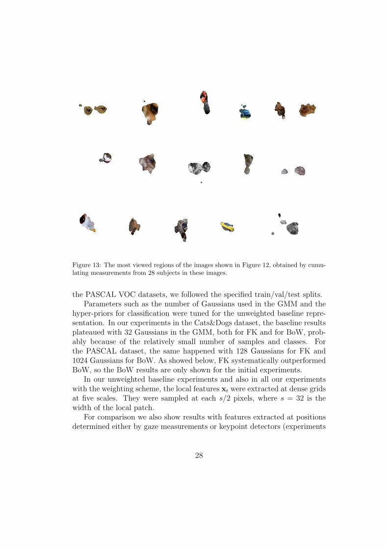
Figure 13: The most viewed regions of the images shown in Figure 12, obtained by cumu-lating measurements from 28 subjects in these images.

the PASCAL VOC datasets, we followed the specified train/val/test splits.Parameters such as the number of Gaussians used in the GMM and the

hyper-priors for classification were tuned for the unweighted baseline repre-sentation. In our experiments in the Cats&Dogs dataset, the baseline resultsplateaued with 32 Gaussians in the GMM, both for FK and for BoW, prob-ably because of the relatively small number of samples and classes. Forthe PASCAL dataset, the same happened with 128 Gaussians for FK and1024 Gaussians for BoW. As showed below, FK systematically outperformedBoW, so the BoW results are only shown for the initial experiments.

In our unweighted baseline experiments and also in all our experimentswith the weighting scheme, the local features xt were extracted at dense gridsat five scales. They were sampled at each s/2 pixels, where s = 32 is thewidth of the local patch.

For comparison we also show results with features extracted at positionsdetermined either by gaze measurements or keypoint detectors (experiments

28

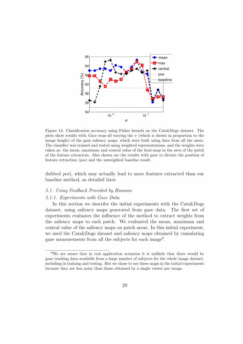
Figure 14: Classification accuracy using Fisher kernels on the Cats&Dogs dataset. Theplots show results with Gaze-map-all varying the σ (which is shown in proportion to theimage height) of the gaze saliency maps, which were built using data from all the users.The classifier was trained and tested using weighted representations, and the weights weretaken as: the mean, maximum and central value of the heat-map in the area of the patchof the feature extractors. Also shown are the results with gaze to dictate the position offeature extraction (pos) and the unweighted baseline result.

dubbed pos), which may actually lead to more features extracted than ourbaseline method, as detailed later.

5.1. Using Feedback Provided by Humans

5.1.1. Experiments with Gaze Data

In this section we describe the initial experiments with the Cats&Dogsdataset, using saliency maps generated from gaze data. The first set ofexperiments evaluates the influence of the method to extract weights fromthe saliency maps to each patch. We evaluated the mean, maximum andcentral value of the saliency maps on patch areas. In this initial experiment,we used the Cats&Dogs dataset and saliency maps obtained by cumulatinggaze measurements from all the subjects for each image9.

9We are aware that in real application scenarios it is unlikely that there would begaze tracking data available from a large number of subjects for the whole image dataset,including in training and testing. But we chose to use these maps in the initial experimentsbecause they are less noisy than those obtained by a single viewer per image.

29

Method BoW Fishermean 52.7 65.3

Gaze-map-all max 54.6 64.9centre 53.1 65.3

unweighted baseline 50.8 55.0

Table 2: The best results (in % of classification accuracy) of each curve shown in Figure 14.In this three class dataset, chance would result in a correct classification rate of 40%, whichis the a priory probability of the most populous classes.

Method BoW Fisherindividual people (Gaze-map-Ind) 50.7 ± 2.9 61.8 ± 2.4

leave-one-out (Gaze-map-LOO) 51.0 ± 2.0 60.9 ± 1.9

Table 3: The best results (in % of classification accuracy) of each curve shown in Figure 15.The unweighted baseline is the same as in Table 2.

Figure 14 shows results obtained with the Fisher kernels representationby computing ψt using the mean, the maximum and the central value of thepatches of each local feature. Table 2 shows the best result of each curve inFigure 14 and it also includes the results obtained with BoW. Figure 14 alsoincludes the result without our weighting scheme, dubbed baseline, which isequivalent to the proposed scheme with uniform weights. As σ gets larger, theresults with the weighted representations start to converge to the baseline,because in this case the weights approach uniformity throughout the images.

These results show that there is no significant difference in the top resultsbetween the different local weighting methods, but the results with meanconsistently stay near its top for a large range of σ values. For this reasonwe used the local mean of the saliency maps to weight patches in the restof this paper. If processing speed is a more important criterion, the centralweighting scheme can be used, as it only requires computing saliency valuesat the patch centres, rather than at all image pixels.

The most important result of Figure 14 and Table 2 is that a significantboost in classification performance was observed with the use of gaze-basedsaliency maps and the proposed weighting scheme with Fisher kernels. Animprovement was also observed with BoW, though it was not as striking.

The next experiments, whose results are shown in Figure 15 and Ta-ble 3, evaluated two possibilities regarding the eye tracking data. In thefirst one, gaze data from a single person is used to generate weight factors

30

(a) Gaze-map-Ind (b) Gaze-map-LOO

Figure 15: Similar to Figure 14, showing results by: (a) using saliency maps built fromgaze data of a single person per image, the same person for training and for testing; and(b) using saliency maps built in a leave-one-person-out scheme. The curves show the meanaccuracy and the error bars show the standard deviation for 11 different people.

for both training and testing images (the Gaze-map-Ind scenario, introducedin Section 3.1). We evaluated this with data from 11 subjects10 and plot-ted the mean and standard deviation of their results varying σ, as shown inFigure 15(a). The results with masks generated in a leave-one-person-outscheme (Gaze-map-LOO) are in Figure 15(b). The later simulates a collabo-rative annotation scenario, in which training images have been viewed by 10users and a new test image is viewed by a new user.

A significant improvement was obtained with weighted Fisher vectors,but the same is not true for BoW, since the BoW representation is not richenough. Notice that there is no significant difference between the best resultsobtained by training and testing with a single person (Gaze-map-Ind) andthe leave-one-out experiments (Gaze-map-LOO). This is explained by thefact that despite minor differences, gaze trajectories share many patternsamong different users when these are exposed to the same images.

As mentioned in Section 3.1, we also show results with an alternativemethod to use gaze data for categorisation: by setting the position of thefeature extractors to be at the centre of the gaze scan-path points. The

10Due to occlusions, head motion and excessive blinking, the eye tracker sometimesgot lost, missing measurements for some images. For these two experiments, we chose todisregard the data of users with whom this happened.

31

Method Accuracy (%)Gaze-pos-Ind 52.4 ± 3.6

Gaze-pos-LOO 51.5 ± 2.4Gaze-pos-all 59.2

Table 4: Classification results on the Cat&Dog dataset using Fisher kernels. Here, resultswith the Gaze-pos methods are shown: features are extracted at the position of gazemeasurements, instead of diffusing them as weights to dense features. For comparison,check the Fisher results with Gaze-map-all-mean (Table 2), Gaze-map-Ind and Gaze-map-

LOO (Table 3). The unweighted method gives 55.0% (as in Table 2).

unweighted representation is then built using these feature vectors. Thisis dubbed pos in Figure 14 and Gaze-pos in Table 2. Note that the resultwith Gaze-pos-all is a significant increase over the unweighted baseline inCats&Dogs. That result is comparable to the results obtained using theproposed weighting scheme (Gaze-maps). In contrast, the results with Gaze-pos-Ind and Gaze-pos-LOO (which are worse than the baseline) show a lack ofrobustness if gaze points are used to set the position of the feature extractionmethods. Our weighting scheme (Gaze-map) also has an advantage in termsof computational complexity. In these experiments, the subjects provideda combined number of 3058 ± 628 points per image, each of these points isused to extract five feature vectors (one for each scale) in the Gaze-pos-allmethod, giving an average of 15,290 feature vectors per image. In contrast,the dense grid used for the baseline and for our method gives an average of1000 feature vectors per image (including all the five scales).

As discussed before, the gaze maps highlight the eyes regions in imagesand these maps lead to a significant improvement in classification perfor-mance. In a qualitative level, this result agrees with early experiments withface recognition, which show that, in human vision the eyes are the mostimportant features for recognition [27], and for computer vision the regionsof the eyes alone have better discrimination power than the whole face [5].

5.1.2. Experiments with Soft Bounding Boxes (SBB)

Bounding boxes around objects of interest are available in the PASCALVOC datasets, and so they are for our Cats&Dogs dataset, which was builtusing a subset of PASCAL VOC2007. We processed the available annotationsto obtain SBBs, as explained in Section 3.1.2. The results are in Table 5,which shows a significant improvement over the unweighted representation in

32

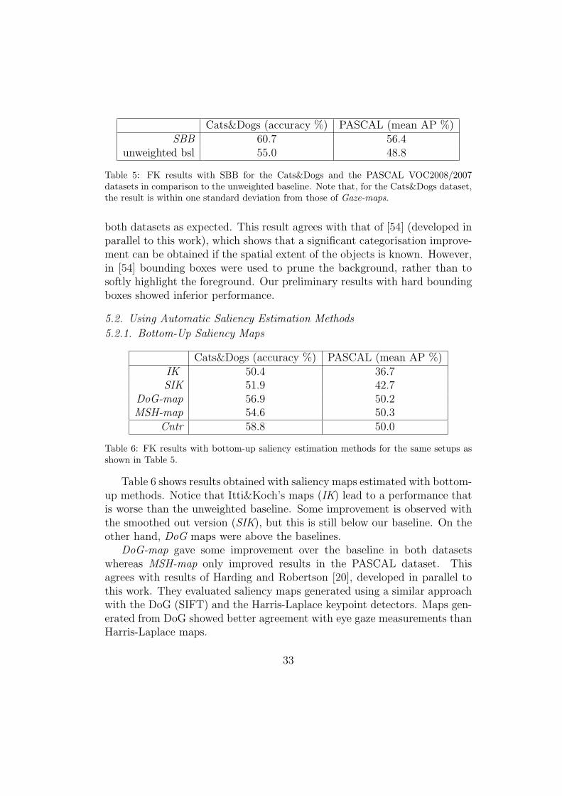
Cats&Dogs (accuracy %) PASCAL (mean AP %)SBB 60.7 56.4

unweighted bsl 55.0 48.8

Table 5: FK results with SBB for the Cats&Dogs and the PASCAL VOC2008/2007datasets in comparison to the unweighted baseline. Note that, for the Cats&Dogs dataset,the result is within one standard deviation from those of Gaze-maps.

both datasets as expected. This result agrees with that of [54] (developed inparallel to this work), which shows that a significant categorisation improve-ment can be obtained if the spatial extent of the objects is known. However,in [54] bounding boxes were used to prune the background, rather than tosoftly highlight the foreground. Our preliminary results with hard boundingboxes showed inferior performance.

5.2. Using Automatic Saliency Estimation Methods

5.2.1. Bottom-Up Saliency Maps

Cats&Dogs (accuracy %) PASCAL (mean AP %)IK 50.4 36.7SIK 51.9 42.7

DoG-map 56.9 50.2MSH-map 54.6 50.3

Cntr 58.8 50.0

Table 6: FK results with bottom-up saliency estimation methods for the same setups asshown in Table 5.

Table 6 shows results obtained with saliency maps estimated with bottom-up methods. Notice that Itti&Koch’s maps (IK) lead to a performance thatis worse than the unweighted baseline. Some improvement is observed withthe smoothed out version (SIK), but this is still below our baseline. On theother hand, DoG maps were above the baselines.

DoG-map gave some improvement over the baseline in both datasetswhereas MSH-map only improved results in the PASCAL dataset. Thisagrees with results of Harding and Robertson [20], developed in parallel tothis work. They evaluated saliency maps generated using a similar approachwith the DoG (SIFT) and the Harris-Laplace keypoint detectors. Maps gen-erated from DoG showed better agreement with eye gaze measurements thanHarris-Laplace maps.

33

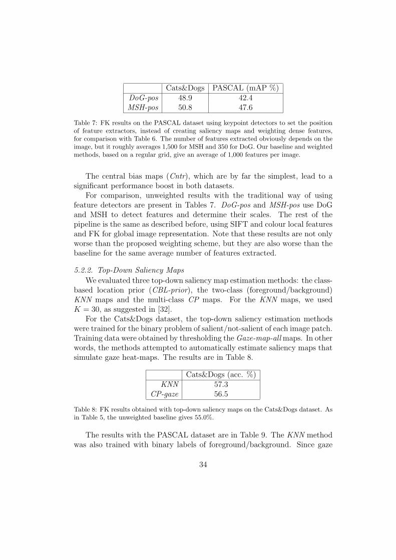
Cats&Dogs PASCAL (mAP %)DoG-pos 48.9 42.4MSH-pos 50.8 47.6

Table 7: FK results on the PASCAL dataset using keypoint detectors to set the positionof feature extractors, instead of creating saliency maps and weighting dense features,for comparison with Table 6. The number of features extracted obviously depends on theimage, but it roughly averages 1,500 for MSH and 350 for DoG. Our baseline and weightedmethods, based on a regular grid, give an average of 1,000 features per image.

The central bias maps (Cntr), which are by far the simplest, lead to asignificant performance boost in both datasets.

For comparison, unweighted results with the traditional way of usingfeature detectors are present in Tables 7. DoG-pos and MSH-pos use DoGand MSH to detect features and determine their scales. The rest of thepipeline is the same as described before, using SIFT and colour local featuresand FK for global image representation. Note that these results are not onlyworse than the proposed weighting scheme, but they are also worse than thebaseline for the same average number of features extracted.

5.2.2. Top-Down Saliency Maps

We evaluated three top-down saliency map estimation methods: the class-based location prior (CBL-prior), the two-class (foreground/background)KNN maps and the multi-class CP maps. For the KNN maps, we usedK = 30, as suggested in [32].

For the Cats&Dogs dataset, the top-down saliency estimation methodswere trained for the binary problem of salient/not-salient of each image patch.Training data were obtained by thresholding the Gaze-map-all maps. In otherwords, the methods attempted to automatically estimate saliency maps thatsimulate gaze heat-maps. The results are in Table 8.

Cats&Dogs (acc. %)KNN 57.3

CP-gaze 56.5

Table 8: FK results obtained with top-down saliency maps on the Cats&Dogs dataset. Asin Table 5, the unweighted baseline gives 55.0%.

The results with the PASCAL dataset are in Table 9. The KNN methodwas also trained with binary labels of foreground/background. Since gaze

34

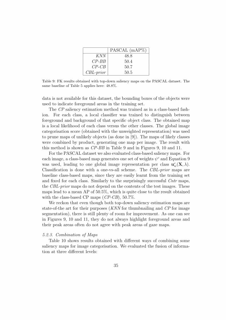
PASCAL (mAP%)KNN 48.8

CP-BB 50.4CP-CB 50.7

CBL-prior 50.5

Table 9: FK results obtained with top-down saliency maps on the PASCAL dataset. Thesame baseline of Table 5 applies here: 48.8%.

data is not available for this dataset, the bounding boxes of the objects wereused to indicate foreground areas in the training set.

The CP saliency estimation method was trained as in a class-based fash-ion. For each class, a local classifier was trained to distinguish betweenforeground and background of that specific object class. The obtained mapis a local likelihood of each class versus the other classes. The global imagecategorisation score (obtained with the unweighted representation) was usedto prune maps of unlikely objects (as done in [9]). The maps of likely classeswere combined by product, generating one map per image. The result withthis method is shown as CP-BB in Table 9 and in Figures 9, 10 and 11.

For the PASCAL dataset we also evaluated class-based saliency maps. Foreach image, a class-based map generates one set of weights ψc and Equation 9was used, leading to one global image representation per class uc

w(X, λ).Classification is done with a one-vs-all scheme. The CBL-prior maps arebaseline class-based maps, since they are easily learnt from the training setand fixed for each class. Similarly to the surprisingly successful Cntr maps,the CBL-prior maps do not depend on the contents of the test images. Thesemaps lead to a mean AP of 50.5%, which is quite close to the result obtainedwith the class-based CP maps (CP-CB), 50.7%.

We reckon that even though both top-down saliency estimation maps arestate-of-the art for their purposes (KNN for thumbnailing and CP for imagesegmentation), there is still plenty of room for improvement. As one can seein Figures 9, 10 and 11, they do not always highlight foreground areas andtheir peak areas often do not agree with peak areas of gaze maps.

5.2.3. Combination of Maps

Table 10 shows results obtained with different ways of combining somesaliency maps for image categorisation. We evaluated the fusion of informa-tion at three different levels:

35

Methods Map fusion Kernel comb. Late fusion individual res.Cntr, DoG 50.6 50.2 50.8 (50.0, 50.2)Cntr, KNN 48.7 50.8 50.2 (50.0, 48.8)DoG, KNN 49.4 50.8 50.4 (50.2, 48.8)

Table 10: Mean average precision (%) results in the PASCAL dataset using combinationsof top-down and bottom-up saliency maps. The unweighted baseline of 48.8% applies here.

• Map fusion: each saliency map is a 2D pdf. Based on an independenceassumption of the maps, the pdfs can be combined via joint probabilityof saliency, given by the pixel-wise product of each map.

• Kernel combination: we did experiments with the simple concatena-tion of image-level descriptors, i.e., FK vectors.

• Late fusion: this is achieved by combining classifier outputs. Since theclassifier used [30] outputs likelihood scores for each class, late fusioncan be done by simply averaging the outputs.

Map product is the less costly but no categorisation improvement was ob-served with this method. The concatenated vectors obviously have higher di-mensionality, which slows down computations depending on the kernel used.Late fusion is the most modular method in terms of implementation, but re-quires the training and testing of two systems. The best results in Table 10are those with late fusion of central bias (Cntr) and the DoG maps. PASCALVOC is very challenging and an improvement of 2% in the mean AUC overthe previous method is significant, but the improvement is relatively smallcompared to the individual result of DoG. We also evaluated combinationsof top-down methods (KNN and CP), but no significant improvement wasobtained, since these two methods are highly correlated to each other, asboth are based on the same local features and FK vectors.

5.3. Computational Complexity

In this section, we discuss the computational complexity of our methodin comparison to other methods based on keypoint detection. The commentshere refer to each relevant step of the pipeline for a test image.

Keypoint detection vs Saliency map computation. These two pro-cesses have similar computational cost. In fact, keypoint detectors normallybuild a saliency map as an intermediate step before outputting local maxima.

36

In this case, bottom-up maps are faster than keypoint detectors. In the caseof the CP top-down method, the cost of saliency estimation is very smallbecause saliency is estimated by applying a regressor on the local statistics(which are used to build the global image representation anyway).

Local feature extraction: keypoint-based vs grid-based. The twomethods can approximately have the same computational cost if the follow-ing conditions are satisfied: (i) the same descriptors are used in both cases,(ii) the number of descriptors is similar, (iii) the descriptors are not affineinvariant, i.e., if the descriptors are not rotation invariant and if the scalein which they are extracted is quantised to the same set of scales used inthe grid-based method. In the latter case, most descriptors can be imple-mented using global image filtering operations at a pre determined set ofscales. This makes feature extraction fast in grid-based methods and canalso be applied to keypoint-based methods, so they would have the samecomputational complexity. However, if the keypoint-based method uses finelocal affine transformations, it becomes more expensive than the grid-basedmethod that we use. The proposed weighting scheme combines the efficiencyadvantage of grid-based feature extraction with the possibility to highlightrelevant image regions done in keypoint-based methods. Recently, some au-thors (e.g. [50]) have combined keypoints and grid-based methods at kernellevel, which means twice the effort at both feature extraction and kernelcomputation.

Global image signature computation: unweighted vs weighted.

As one can see from Equation 2, the only additional cost of using the weightedrepresentation is an additional scalar multiplication ψt associated to thestatistics of each local feature gt, where ψt is obtained from the saliencymap. In [44], we show that the weighting scheme proposed here can be seenas an alternative to spatial pyramid kernels (SP). The goal of SP is to softencode location information in the global image signature. Our method com-pensates for variations caused by translation of local image features in imagesof the same objects if their local weights are preserved. We show in [44] thatthe scheme proposed here leads to better performance than SPs with imagesignatures that are 1/8 of the size of those of SPs. This has a direct impacton the speed of the kernel computation for classification.

Kernel computations. The winners of the PASCAL VOC challengesin 2009 and 2010 have used object detection to aid image categorisation [15,14]. The latter (2010) combine detection results and global image signaturesvia MKL. Kernel computation (which involves computing distance between

37

high dimensional vectors) is obviously more expensive than weighted voting(which is just one scalar multiplication).

6. Concluding Remarks

6.1. Summary and Discussion

We introduced a novel image representation in which images are modelledas order-less sets of weighted low-level local features. We showed how to in-tegrate this framework in bag-of-features representations. This consists inaccumulating weighted statistics computed at the patch level. The weightscan be computed from visual saliency maps and the experiments presentedhere explored this possibility with different saliency map computation meth-ods, including methods that use feedback from people and fully automaticmethods. Two bag-of-features representations have been evaluated, the pop-ular bag-of-visual-words (BoW) with soft voting and the Fisher kernels (FK)representation of [41]. The later consistently outperforms the former andit has shown a more significant boost in performance using the proposedweighted representation.

We evaluated our method for image categorisation, but the obtained vec-torial representation can also be applied for tasks such as image retrievaland clustering. To our knowledge, this is the first paper which makes use ofsaliency maps for a generic method of image categorisation. Previous workhave used gaze data in methods that are crafted for detection of specificcategories [23].

We showed on a small dataset that our method could significantly benefitfrom gaze tracking data. Similarly, a significant improvement is achievedusing saliency maps based on soft-bounding boxes (SBB) created using ex-plicit feedback from users. The SBB also lead to a significant performanceimprovement in the PASCAL VOC2008/2007 dataset. This result, obtainedwith only two types of low level features (colour and SIFT) is slightly betterthan that obtained by the UvA Soft5ColourSift method, one of the winners ofPASCAL 2008, which reported an average AP of 55.8% [13], against 56.7% ofour method with SBB for the experiment on PASCAL2007 test data. Notethat UvA Soft5ColourSift used a system with many channels and combi-nation at kernel level using MKL. Such a system might be too costly forpractical applications. On the other hand this is not a fair comparison, sincetheir method does not use any explicit feedback.

38

Automatic bottom-up saliency maps based on difference of Gaussians [31](DoG) also gave some improvement on both datasets with our method. Morestriking, the simplest method of central bias leads to relatively high improve-ments. This is in agreement with one of the results of [25], which shows thatthe central bias is among the best predictors for visual attention. On theother hand, Itti&Koch’s maps [22] lead to disappointing results. This issomewhat expected as Foulsham and Underwood [17] showed that the meanproportion of eye fixations that land on regions marked as salient by [22] isonly 20% (where random guess would score around 10%).

We compared the results obtained with saliency maps built from key-points (detected automatically or measured by a gaze tracker) versus the useof those keypoints to directly drive the position to extract feature vectors.The proposed approach, which use saliency maps to weight features, lead tobetter results.

We also explored some top-down saliency estimation methods based ona state-of-the-art segmentation method [9] (CP) and on a recent automaticthumbnailing method [32] (KNN). The former (CP) lead to better perfor-mances, but this was followed closely by the use of maps generated by simpleclass-based object location prior (CBL-prior), which do not depend on theimage content.

The combination of some methods was also explored: central bias, DoGand KNN. The best result, combining the central bias with DoG was a meanaverage precision of 50.8% in the PASCAL dataset, 2% better than the un-weighted method. Note that 2% improvement is quite an achievement forthe PASCAL datasets. Usually the results of the top three or four methodsof PASCAL challenges are within 2% of mean AP from each other.

Since the use of different saliency maps only affect the cumulation ofstatistics to compute the vectorial representation, several saliency maps canbe used for each image, implying no additional cost for feature extraction andcomputation of patch statistics (the local features xt and their representationgt can be pre-computed and stored in a database). This constitutes a keyadvantage of our method w.r.t. methods based on sampling density. This isalso an advantage considering that gaze tracking devices may become popularin the future and can be used to boost semi-automatic image annotation andretrieval. At application time, only the local weights are adjusted to neweye gaze data and the remaining computations (statistics accumulation andclassification) are very fast in comparison.

39

6.2. Follow-up work

Our results have pointed that although gaze-based saliency maps givethe most significant performance boost, for the task of image categorisation,maps that highlight objects seem to lead to better performance improve-ment than maps that try to mimic human visual attention. Therefore, as afollow-up of this work, in [44] we have done further evaluations of the locallyweighted features idea using the objectness measure of Alexe et al. [1] togenerate saliency maps. We argued that the proposed method is a way tomodel spatial layout in images and showed that this weighting scheme usingthe objectness measure reduces the within-class variance and therefore leadsto improved classification results in the PASCAL VOC datasets.

In the experiments, we used the improvements for the Fisher Kernelsmethod proposed in [42] to build image signatures both using the schemeproposed here and the popular Spatial Pyramid Kernels (SPs). The resultsshow that our method outperforms SPs with image signatures that are 1/8of their size: in the PASCAL 2007 dataset, the unweighted Fisher Kernels(baseline) method gave a mean AP of 62.7%, SPs gave 63.8% and our methodgave 64.5%. The previous state-of-the-art was that of [65]: 64.0%. Whenour method is combined with SPs and a simple method that encodes locationinformation as part of the local feature vectors, our results reset the state-of-the-art in PASCAL VOC2007,2008 and 2009.

Future work includes the use of information about the context of theimage (e.g. paintings, landscapes, flowers) and the context of the task (e.g.object detection, scene classification, image retrieval) as priors on saliencymaps.

Acknowledgements

The research leading to these results has received funding from the Eu-ropean Community’s Seventh Framework Programme (FP7/2007–2013) un-der grant agreement n◦ 216529, Personal Information Navigator AdaptingThrough Viewing, PinView. TdC was also supported by the EPSRC projectACASVA (UK) while writing this paper.

We acknowledge Craig Saunders for his aid on setting up the gaze trackingexperiments and all the Xerox employees who kindly participated on the eyemovements data collection.

40

[1] Alexe, B., Deselaers, T., Ferrari, V.: What is an object? In: Proc IEEEConf on Computer Vision and Pattern Recognition, San Francisco, CA,June 13-18 (2010)

[2] Boureau, Y.L., Ponce, J., LeCun, Y.: A theoretical analysis of featurepooling in visual recognition. In: Proc. of the 27th International confer-ence on Machine Learning (ICML). Haifa, Israel (2010)

[3] Bruce, N.D., Tsotsos, J.K.: Saliency, attention, and visual search: Aninformation theoretic approach. Journal of Vision 9(3), 5, 1–24 (2009)

[4] de Campos, T.: Description and evaluation of novel local featureswith usable sub-categorisation performance. Tech. rep., PinView Eu-ropean Community project FP7-216529 (2008). D6.1, available athttp://www.pinview.eu

[5] de Campos, T., Feris, R., Cesar, R.: Eigenfaces versus eigeneyes: Firststeps toward performance assessment of representations for face recog-nition. In: MICAI, LNCS, vol. 1793, pp. 197–206. Acapulco, Mexico(2000)

[6] Chang, E., Mallat, S., Yap, C.: Wavelet foveation. Journal of Appliedand Computational Harmonic Analysis 9, 312–335 (2000)

[7] Chen, L.Q., Xie, X., Fan, X., Ma, W.Y., Zhang, H.J., Zhou, H.Q.: Avisual attention model for adapting images on small displays. ACMMultimedia Systems Journal 9(4) (2003)

[8] Csurka, G., Dance, C.R., Fan, L., Willamowski, J., Bray, C.: Visual cat-egorization with bags of keypoints. In: ECCV International Workshopon Statistical Learning in Computer Vision (2004)

[9] Csurka, G., Perronnin, F.: A simple high performance approach to se-mantic segmentation. In: BMVC (2008)

[10] Einhauser, W., Spain, M., Perona, P.: Objects predict fixations bet-ter than early saliency. Journal of Vision 8(14:18), 1–26 (2008).Http://journalofvision.org/8/14/18/

[11] Elson, J., Douceur, J.R., Howell, J., Saul, J.: A CAPTCHA that exploitsinterest-aligned manual image categorization. In: 14th ACM Conferenceon Computer and Communications Security (CCS) (2007)

41

[12] Everingham, M., Gool, L.V., Williams, C.K.I., Winn,J., Zisserman, A.: The PASCAL Visual Object ClassesChallenge 2007 (VOC2007) Results. http://www.pascal-network.org/challenges/VOC/voc2007/workshop/index.html (2007)

[13] Everingham, M., Gool, L.V., Williams, C.K.I., Winn,J., Zisserman, A.: The PASCAL Visual Object ClassesChallenge 2008 (VOC2008) Results. http://www.pascal-network.org/challenges/VOC/voc2008/workshop/index.html (2008)

[14] Everingham, M., Van Gool, L., Williams, C.K.I., Winn,J., Zisserman, A.: The PASCAL Visual Object ClassesChallenge 2010 (VOC2010) Results. http://www.pascal-network.org/challenges/VOC/voc2010/workshop/index.html

[15] Everingham, M., Van Gool, L., Williams, C.K.I., Winn,J., Zisserman, A.: The PASCAL Visual Object ClassesChallenge 2009 (VOC2009) Results. http://www.pascal-network.org/challenges/VOC/voc2009/workshop/index.html (2009)

[16] Farqhar, J.D.R., Szedmak, S., Meng, H., Shawe-Taylor, J.: Improving“bag-of-keypoints” image categorisation: Generative models and pdf-kernels. Tech. rep., University of Southampton (2005). LAVA project,European Union

[17] Foulsham, T., Underwood, G.: What can saliency models predict abouteye movements? spatial and sequential aspects of fixations during en-coding and recognition. Journal of Vision 8(2), 1–17 (2008)

[18] Frintrop, S., Rome, E., Christensen, H.: Computational visual attentionsystems and their cognitive foundation: A survey. ACM Transactionson Applied Perception (2009)

[19] van Gemert, J.C., Veenman, C.J., Smeulders, A.W.M., Geusebroek,J.M.: Visual word ambiguity. IEEE Transactions on Pattern Analysisand Machine Intelligence 32(7), 1271–1283 (2010)

[20] Harding, P., Robertson, N.: A comparison of feature detectors withpassive and task-based visual saliency. In: Proc Scandinavian Confer-ence on Image Analysis, no. 5575 in LNCS, pp. 714–725. Springer, Oslo(2009)

42

[21] Harris, C., Stephens, M.: A combined corner and edge detector. In:Proc 4th Alvey Vision Conf, Manchester, pp. 147–151 (1988)

[22] Itti, L., Koch, C.: A saliency-based search mechanism for overt andcovert shifts of visual attention. Vision Research 40, 1489–1506 (2000)

[23] Jaimes, A., Pelz, J., Grabowski, T., Babcock, J., Chang, S.F.: Usinghuman observers’ eye movements in automatic image classifiers. In:proc. SPIE conference on Human Vision and Electronic Imaging VI.San Jose, CA (2001)

[24] Jegou, H., Douze, M., Schmid, C.: On the burstiness of visual elements.In: Proc IEEE Conf on Computer Vision and Pattern Recognition, Mi-ami Beach, FL, June 20-25 (2009)

[25] Judd, T., Ehinger, K., Durand, F., Torralba, A.: Learning to predictwhere humans look. In: Proc 12th Int Conf on Computer Vision, Kyoto,Japan, Sept 29 - Oct 2 (2009)

[26] Kadir, T., Brady, M.: Scale, saliency and image description. IJCV45(2), 83–105 (2001)

[27] Keil, M.S.: “I look in your eyes, honey”: Internal face features inducespatial frequency preference for human face processing. PLoS Compu-tational Biology 5(3) (2009)

[28] Kienzle, W., Wichmann, F.A., Scholkopf, B., Franz, M.O.: A nonpara-metric approach to bottom-up visual saliency. In: Proc of the NeuralInformation Processing Systems (NIPS), pp. 689–698 (2007)

[29] Kootstra, G., Nederveen, A., de Boer, B.: Paying attention to symmetry.In: BMVC (2008)

[30] Krishnapuram, B., Carin, L., Figueiredo, M., Hastemink, A.: Sparsemultimodal logistic regression: Fast algorithms and generalizationbounds. IEEE PAMI 27(6) (2005)

[31] Lowe, D.G.: Distinctive image features from scale-invariant keypoints.IJCV 60(2) (2004)

43

[32] Marchesotti, L., Cifarelli, C., Csurka, G.: A framework for visualsaliency detection with applications to image thumbnailing. In: Proc12th Int Conf on Computer Vision, Kyoto, Japan, Sept 29 - Oct 2(2009)

[33] Mikolajczyk, K., Schmid, C.: Scale and affine invariant interest pointdetectors. IJCV 60(1) (2004)

[34] Mikolajczyk, K., Schmid, C.: A performance evaluation of local descrip-tors. IEEE PAMI 27(10) (2005)

[35] Moosmann, F., Larlus, D., Jurie, F.: Learning saliency maps for objectcategorization. In: ECCV International Workshop on The Representa-tion and Use of Prior Knowledge in Vision. Springer (2006)

[36] Nilsback, M.E., Zisserman, A.: Automated flower classification over alarge number of classes. In: Proc. of the Indian Conference on ComputerVision, Graphics and Image Processing (2008)

[37] Nowak, E., Jurie, F., Triggs, W.: Sampling strategies for bag-of-featuresimage classification. In: ECCV (2006)

[38] Oyekoya, O.: Eye tracking: A perceptual interface for content basedimage retrieval. Ph.D. thesis, DEEE, University College London (2007)

[39] Parikh, D., Lawrence Zitnick, C., Chen, T.: Determining patch saliencyusing low-level context. In: ECCV (2008)

[40] Perronnin, F.: Universal and adapted vocabularies for generic visualcategorization. IEEE Transactions on Pattern Analysis and MachineIntelligence 30(7), 1243–1256 (2008)

[41] Perronnin, F., Dance, C.: Fisher kernel on visual vocabularies for imagecategorization. In: CVPR (2007)

[42] Perronnin, F., Sanchez, J., Mensink, T.: Improving the Fisher kernelfor large-scale image classification. In: Proc 11th European Conf onComputer Vision, Crete, Greece, September 5-11, vol. 4, pp. 143–156(2010)

[43] Rutishauser, U., Walther, D., Koch, C., Perona, P.: Is bottom-up at-tention useful for object recognition? In: CVPR (2004)

44

[44] Sanchez, J., Perronnin, F., de Campos, T.: Modeling the spatial layoutof images beyond spatial pyramids. In: Proc 12th Int Conf on ComputerVision, Barcelona, Spain, Nov 6-13 (2011). Submitted

[45] Saunders, C., Klami, A.: Database of eye-movement recordings. Tech.rep., PinView European Community project FP7-216529 (2008). D8.3,available at http://www.pinview.eu

[46] Sivic, J., Zisserman, A.: Video Google: A text retrieval approach toobject matching in videos. In: ICCV (2003)

[47] Stentiford, F.W.M.: Attention based similarity. Pattern Recognition40(3), 771–783 (2007)

[48] Suh, B., Ling, H., Bederson, B., Jacobs, D.: Thumbnail cropping and itseffectiveness. In: ACM User Interface Software and Technology (2003)

[49] Sundstedt, V., Chalmers, A., Cater, K., Debattista, K.: Top-down visualattention for efficient rendering of task related scenes. In: In Vision,Modeling and Visualization, pp. 209–216 (2004)

[50] Tahir, M.A., et al: UvA & Surrey @ PASCAL 2008 (2008). VisualRecognition Challange workshop, in conjunction with ECCV

[51] Tatler, B.W.: The central fixation bias in scene viewing: Selecting anoptimal viewing position independently of motor biases and image fea-ture distributions. Journal of Vision 7(14:4), 1–17 (2007)

[52] Torralba, A.: Modeling global scene factors in attention. Journal ofOptical Society of America A. Special Issue on Bayesian and StatisticalApproaches to Vision 20(7), 1407–1418 (2003)

[53] Torralba, A., Oliva, A., Castelhano, M., Henderson, J.: Contextualguidance of eye movements and attention in real-world scenes: The roleof global features on object search. Psychological Review 113(4), 766–786 (2006)

[54] Uijlings, J.R.R., Smeulders, A.W.M., Scha, R.J.H.: What is the spatialextent of an object? In: Proc IEEE Conf on Computer Vision andPattern Recognition, Miami Beach, FL, June 20-25 (2009)

45

[55] Vedald, A., Gulshan, V., Varma, M., Zisserman, A.: Multiple kernels forobject detection. In: Proc 12th Int Conf on Computer Vision, Kyoto,Japan, Sept 29 - Oct 2 (2009)

[56] Vidal-Naquet, M., Ullman, S.: Object recognition with informative fea-tures and linear classification. In: ICCV (2003)

[57] Viitaniemi, V., Laaksonen, J.: Use of image regions in context-adaptiveimage classification. In: International Conference on Semantic and Dig-ital Media Technologies (SAMT 2006), LNCS, pp. 169–183. Springer,Athens, Greece (2006)

[58] Viitaniemi, V., Laaksonen, J.: Spatial extensions to bag of visualwords. In: ACM International Conference on Image and Video Retrieval(CIVR). Santorini, Greece (2009)

[59] Walther, D., Koch, C.: Modeling attention to salient proto-objects. Neu-ral Networks 19, 1395–1407 (2006)

[60] Wang, G., Forsyth, D.: Joint learning of visual attributes, object classesand visual saliency. In: Proc 12th Int Conf on Computer Vision, Kyoto,Japan, Sept 29 - Oct 2 (2009)

[61] Wang, W., Wang, Y., Huang, Q., Gao, W.: Measuring visual saliency bysite entropy rate. In: Proc IEEE Conf on Computer Vision and PatternRecognition, San Francisco, CA, June 13-18 (2010)

[62] Wang, Z., Li, B.: A two-stage approach to saliency detection in images.In: ICASSP (2008)

[63] Winn, J., Criminisi, A., Minka, T.: Object categorization by learneduniversal visual dictionary. In: Proc 10th Int Conf on Computer Vision,Beijing, China, Oct 15-21 (2005)

[64] Zhang, J., Marsza lek, M., Lazebnik, S., Schmid, C.: Local features andkernels for classification of texture and object categories: a comprehen-sive study. IJCV 73(2) (2007)

[65] Zhou, X., Yu, K., Zhang, T., Huang, T.S.: Image classification usingsuper-vector coding of local image descriptors. In: Proc 11th EuropeanConf on Computer Vision, Crete, Greece, September 5-11 (2010)

46