image target identification of uav based on sift
TRANSCRIPT
Procedia Engineering 15 (2011) 3205 – 3209
1877-7058 © 2011 Published by Elsevier Ltd.doi:10.1016/j.proeng.2011.08.602
Available online at www.sciencedirect.comAvailable online at www.sciencedirect.com
ProcediaEngineering
Procedia Engineering 00 (2011) 000–000
www.elsevier.com/locate/procedia
Advanced in Control Engineeringand Information Science
Image Target Identification of UAV Based on SIFT
Xi Chao-jian*,Guo San-xue Engineering College of Chinese People’s Armed Police Force , Xi’an Shaanxi Province,710086, China
Abstract
The paper finds a method to meet the large amounts of information and real-time processing of the UAV(Unmanned Aerial Vehicle) image, it could increase efficiency of target identification. The SIFT algorithm has good robustness, it could overcome some affect of image deformation and block, but it could not meet the real-time processing of UAV image. The paper use simplified Forstner operator to improve SIFT algorithm, reduce the computation of feature point recognition. Through the simulation, we prove that the improved SIFT algorithm could meet the accuracy and speed requirements of UAV image in the complex background.
© 2011 Published by Elsevier Ltd. Selection and/or peer-review under responsibility of [CEIS 2011]
Keywords: target identification; SIFT; Forstner; Difference Of Gaussian SCALE-SPACE
1. Introduction
UAV is now widely used for aerial image acquisition, transmission and recognition, UAV in flight altitude, flight distance, flight time and task load, and so has incomparable superiority, because of this the information of UAV im a age is correspondingly larger, so the rapid identification of UAV images becomes the goal of continuous pursuit.[1]
Traditional target identification method is based on the global characteristics match, it’s hard to identify and matching at target was partly occlusion or produce deformation[2]. The target recognition based on local features of ways to become solve the above problem effectively. In 2004 Lowe proposed
* Corresponding author,Tel:+8615319796753 Email:[email protected]
3206 Xi Chao-jian and Guo San-xue / Procedia Engineering 15 (2011) 3205 – 32092 Xi Chao-jian et al/ Procedia Engineering 00 (2011) 000–000
SIFT(Scale Invariant Features Transform) based on the partial feature[3]. This algorithm is based on the extreme value of scale space as features points. Meanwhile calculate gradient direction of neighbourhood as the eigenvalue of the point, then match the images based on the eigenvalue as the matching data. The algorithm has strong robustness to deformation, shelter and other influence. However the computation of the algorithm is relative large. So the improvement in order to improve the speed and accuracy, to meet the UAV image recognition requirements.
According to the characteristics of UAV image, analyzes the SIFT algorithm based on scale space and image pyramid method, Forstner operator is introduced to optimize the process of extracting eigenvalue. Forstner are widely used in visual field and photogrammetry, based on the error ellipse to extract target feature point. Compared with Moravec and Hannah, Forstner operator has higher precision and lower complexity. Using differential operator to extract primary points, then using Forstner operator to filter the feature points. Calculating their characteristic vector and matching [4].
2. SIFT algorithm and improved
2.1 Scale space of image
Scale space theory is to emulate the multi-scale features of image data. Koenderink proved that Gaussian convolution is the only linear kernel to achieve scale transformation[5]. The scale space of image can be defined as
( , , ) ( , , )* ( , )L x y G x y I x yσ σ= (1)2 2( )
22
2
1( , , )2
x ye
G x y σσπσ
− +
= (2)
Where (x,y) is space coordinates, is scale coordinates, is Scale variable Gaussian function.
σ ( , , )G x y σ
In order to achieve stable key points testing in scale space, using Gaussian difference kernel of different scale space to do convolution with image, then generating DOG(Difference Of Gaussian SCALE-SPACE)[6].
( , , ) ( ( , , ) ( , , )) * ( , ) ( , , ) ( , , )D x y G x y k G x y I x y L x y k L x yσ σ σ σ= − = − σ (3)
2.2 Construct image pyramid
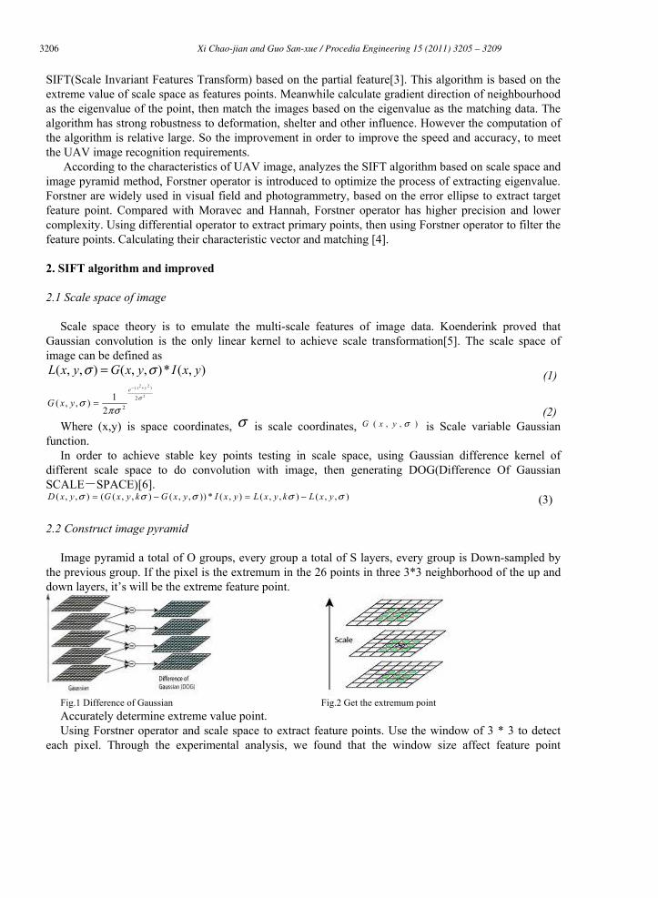
Image pyramid a total of O groups, every group a total of S layers, every group is Down-sampled by the previous group. If the pixel is the extremum in the 26 points in three 3*3 neighborhood of the up and down layers, it’s will be the extreme feature point.
Fig.1 Difference of Gaussian Fig.2 Get the extremum pointAccurately determine extreme value point. Using Forstner operator and scale space to extract feature points. Use the window of 3 * 3 to detect
each pixel. Through the experimental analysis, we found that the window size affect feature point

3207Xi Chao-jian and Guo San-xue / Procedia Engineering 15 (2011) 3205 – 3209Xi Chao-jian et al / Procedia Engineering 00 (2011) 000–000 3
extraction. When the window is bigger easy to lose some feature points, experimental proof that take 3 * 3 window to extract, the point features is more apparent.
Calculate the absolute value of the feature point up, down, right and left. 1 , 1,
2 , ,
3 , 1,
4 , ,
x y x y
x y x y
x y x y
x y x y
g g g
g g g
g g g
g g g
+
+
−
−
⎧ = −⎪⎪ = −⎪⎨
= −⎪⎪
= −⎪⎩
1
1 (4)Take its absolute mean { }1 2 3 4, , ,M m id g g g g= , set absolute threshold T, if M>T, we think it is
primary points. Calculating Roberts gradient Gu and Gv of the (x,y), generating the autocorrelation matrix by Variance
and Covariance of the Gradient. We can calculate the size and shape of the error ellipse through the eigenvalue of the matrix. Based the error ellipse we can find the target feature points.
Roberts gradient: //
u
v
G gG g
= ∂ ∂⎧⎨ = ∂ ∂⎩
uv (5)
The Covariance matrix N of the 3*3 window: 2
2u vu
u v v
G GGN
G G G∑∑
=∑ ∑ (6)
The roundness threshold of the error ellipse q and the extremum of the point w:
2
4 d e t( )d e t
NqtrN
NwtrN
⎧ =⎪⎪⎨⎪ =⎪⎩ (7)
detN is the Determinant matrix N, trN is the algebraic sum of the matrix N, , . In fact, q is the shape of the error ellipse, is the size of the error ellipse.
0ω > 0 1q≤ ≤ω
, 0 .5 1 ., 5w
c
f fT
c cϖω
= −⎧= ⎨ =⎩
ω
5
(8)ϖ is the median, is the average. If q>Tq, , the pixel will be the primary point. In order to
eliminate the influence of rotation and zooming and enhance the robustness of the algorithms[7], we could calculate the convolution of the Roberts gradient and the partial derivative of the Gaussian kernel. Matrix N is transformed to:
c Tωω >
2
2
u u v vu u
u u v v v v
g G g Gg GN
g G g G g G
⎡ ⎤= ⎢ ⎥⎢⎣
∑∑∑ ∑ ⎥⎦ (9)
2.3 Specify the direction of the feature points
To specify the gradient direction feature points based on the local gradient direction of the feature point. Gradient magnitude m and direction θ:
2 2( , ) ( ( 1, ) ( 1), ) ( ( , 1) ( , 1))( , 1) ( , 1)( , ) arctan( 1, ) ( 1, )
m x y L x y L x y L x y L x yL x y L x yx yL x y L x y
θ
= + − − + + − −+ − −=
+ − − (10)
In the actual calculation process, we sampled in a the neighborhood of the point (x, y), the Gradient direction of the pixel could be expressed by the way of histogram statistics, the range of the gradient
3208 Xi Chao-jian and Guo San-xue / Procedia Engineering 15 (2011) 3205 – 32094 Xi Chao-jian et al/ Procedia Engineering 00 (2011) 000–000
histogram is 0°~360°, every 10°a column, it’s could be divide into 36 columns. The principal direction of the neighborhood is the histogram peak. that the direction of the feature point. There are three messages for each feature point, position, scale and direction.
2.4 Generate descriptor of SIFT feature points
Rotate the axis to be in the same direction with the feature point[8], in order to ensure the rotation invariance of image. Select the 8 * 8 window with the feature as the center. As Fig.3 shown.
Fig.3 Gradient direction of neighborhood Calculate the gradient direction histogram of 8 directions in every 4*4 window, so we can get the
superimposed values of gradient direction. A feature point formed by the four factors, each factor has 8 direction vector information, 16 4*4 windows have 128 vector descriptors, they form the SIFT eigenvector. Then we can remove the influence of the light and the contrast by normalizing the eigenvectors.
2.5 SIFT Image matching
We can calculate the Euclidean distance of the eigenvector, then judge the similarity of the two points. We can take a point A in picture 1 and find a point B that the Euclidean distance is minimum distance to the point A in picture 2. If the ratio of the minimum distance and the second smallest distance less than the threshold, we think that the two points is matched[9]. The threshold Lowe recommended is 0.8[10].
3. Experimental analysis
The Experimental platform is formed by a PC(windows XP, CPU E6300, RAM 1G, MATLAB 7.0. According to the above experiment steps, compare the SIFT algorithm improved by the Forstner operator with the traditional SIFT algorithm. The platform identified many images that shot by low-flying UAV. These images are subject to different degrees of rotation, scaling, brightness and noise. Matching rate is above 90% under the condition of rough matching.
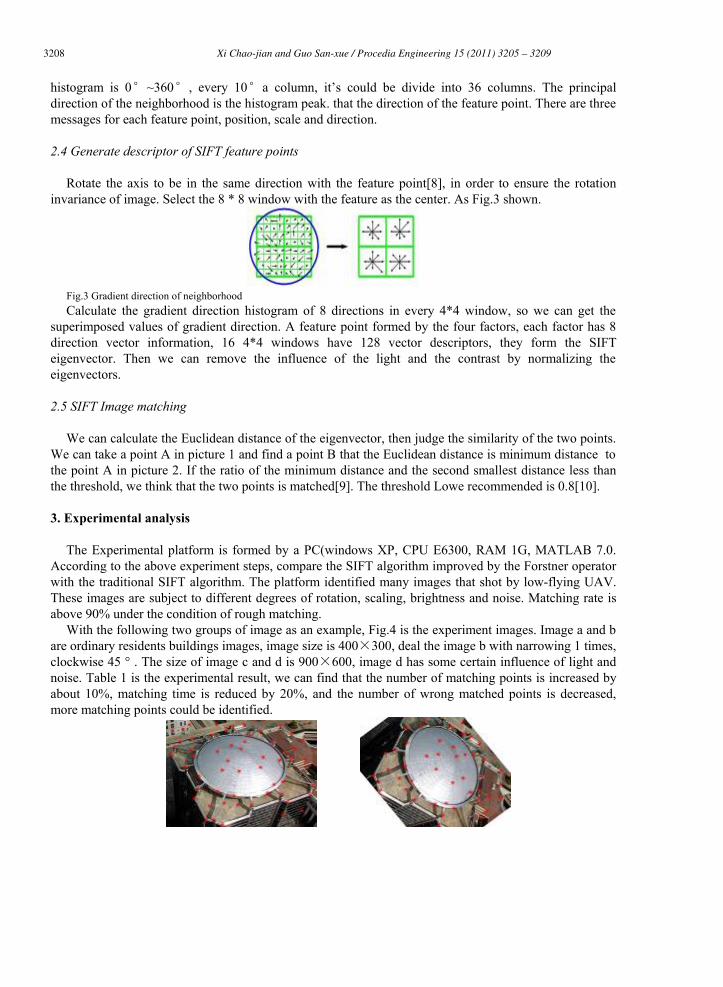
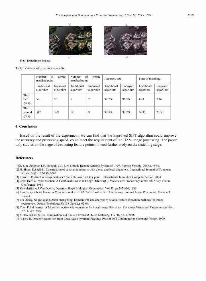
With the following two groups of image as an example, Fig.4 is the experiment images. Image a and b are ordinary residents buildings images, image size is 400×300, deal the image b with narrowing 1 times, clockwise 45 ° . The size of image c and d is 900×600, image d has some certain influence of light and noise. Table 1 is the experimental result, we can find that the number of matching points is increased by about 10%, matching time is reduced by 20%, and the number of wrong matched points is decreased, more matching points could be identified.
3209Xi Chao-jian and Guo San-xue / Procedia Engineering 15 (2011) 3205 – 3209Xi Chao-jian et al / Procedia Engineering 00 (2011) 000–000 5
a b
c d Fig.4 Experiment images
Table 1 Contrast of experimental results
Number of correct matched point
Number of wrong matched point Accuracy rate Time of matching
Traditionalalgorithm
Improved algorithm
Traditionalalgorithm
Improved algorithm
Traditionalalgorithm
Improved algorithm
Traditionalalgorithm
Improved algorithm
The first group
52 56 5 2 91.2% 96.5% 4.23 3.16
The secondgroup
347 389 19 9 92.3% 97.7% 24.35 21.53
4. Conclusion
Based on the result of the experiment, we can find that the improved SIFT algorithm could improve the accuracy and processing speed, could meet the requirement of the UAV image processing. The paper only studies on the stage of extracting feature points, it need further study on the matching stage.
References
[1]Jie Sun, Zongjian Lin, Hongxia Cui, Low altitude Remote Sensing System of UAV. Remote Sensing. 2003.1,49-50. [2] H. Shum, R,Szeliski. Construction of panoramic mosaics with global and local alignment. International Journal of Computer
Vision, 36(2):102-130, 2000 [3] Lowe D. Distinctive image features from scale-invariant key point. International Journal on Computer Vision. 2004 [4] Chris Harris,Mike Stephen. A Combined Corner and Edge Detector[C]. Manchester: Proceedings of the 4th Alvey Vision
Conference. 1988 [5] Koenderink A.J.Van Doorm, Dynamic Shape Biological Cybernetics. Vol.53, pp.383-396, 1986 [6] Luo Juan, Oubong Gwun. A Comparison of SIFT PAC-SIFT and SURF. International Journal Image Processing; Volume 3,
Issue 4. [7] Liu Qiong, Ni guo-qiang, Zhou Sheng-bing. Experiments and analysis of several feature extraction methods for image
registration. Optical Technique; Vol.33 Num.1,p.62-64. [8] Y.ke, R.Snkthankar. A More Distinctive Representation for Local Image Descriptor. Computer Vision and Pattern recognition.
P.511-517. 2004. [9] Y.Heo, K.Lee, S.Lee. Illumination and Camera Invariant Stereo Matching, CVPR. p 1-8. 2008 [10] Lowe D. Object Recognition from Local Scale Invariant Features. Proc.of Int’l Conference on Computer Vision. 1999.